跳到论文正文
W Papers独立论文阅读器 arXiv:2012.10278 论文正文 计算阅读时间 · 0%
引用这篇论文根据当前论文元数据生成,正式投稿前建议核对。


License: CC BY 4.0
arXiv:2012.10278v1 [stat.ML] 18 Dec 2020

Adversarially Robust Estimate and Risk Analysis in Linear Regression

Yue Xing Affiliation: Department of Statistics, Purdue University    Ruizhi Zhang Affiliation: Department of Statistics, University of Nebraska-Lincoln    Guang Cheng Affiliation: Department of Statistics, Purdue University
Abstract

Adversarially robust learning aims to design algorithms that are robust to small adversarial perturbations on input variables. Beyond the existing studies on the predictive performance to adversarial samples, our goal is to understand statistical properties of adversarially robust estimates and analyze adversarial risk in the setup of linear regression models. By discovering the statistical minimax rate of convergence of adversarially robust estimators, we emphasize the importance of incorporating model information, e.g., sparsity, in adversarially robust learning. Further, we reveal an explicit connection of adversarial and standard estimates, and propose a straightforward two-stage adversarial learning framework, which facilitates to utilize model structure information to improve adversarial robustness. In theory, the consistency of the adversarially robust estimator is proven and its Bahadur representation is also developed for the statistical inference purpose. The proposed estimator converges in a sharp rate under either low-dimensional or sparse scenario. Moreover, our theory confirms two phenomena in adversarially robust learning: adversarial robustness hurts generalization, and unlabeled data help improve the generalization. In the end, we conduct numerical simulations to verify our theory.

1 Introduction

The development of machine/deep learning methods has led to breakthrough performance in various areas of application. However, some recent research revealed that these powerful but delicate models are vulnerable to random perturbation and adversarial attacks. For example, well-designed malicious adversarial input may induce wrong decision making when filtering junk emails or detecting malicious binary programs [41, 23]. On the other hand, by studying adversarial samples, one can in turn improve adversarial robustness of algorithms in practice. The existing literature focus on generating adversarial samples, e.g., [24, 23], adversarial training, e.g., [10, 17, 32], invariance/interpretability to detect adversarial samples, e.g., [37, 30, 18, 9, 6] and theoretical studies of adversarially robust learning, e.g., [34, 35, 36]. In particular, some studies [39, 25] showed that adversarial training leads to a worse generalization performance, while [27, 40, 21] argued that the adversarial robustness requires more (labeled/unlabeled) data to enhance generalization performance. In addition, the trade-off between standard performance and adversarial performance is carefully characterized in [42, 15].

Adversarially robust estimation in the literature is often formulated as an empirical “min-max” problem: minimizing the empirical risk under the worst-case attack (which maximizes the loss) on the training data. Unfortunately, this formulation has not directly taken into account the structural information of the model such as sparsity and grouping, e.g., [28, 29, 32], which may be utilized to improve adversarial robustness. This is particularly needed in the high-dimensional regime, i.e., data dimension pp is much larger than sample size nn, where the empirical (adversarial) risk may no longer converge to the population risk [19].

The above concern raises two questions: (1) whether the statistical minimax11 1 In this paper, “min-max” refers to the optimization problem considered in adversarially robust learning, while “minimax” refers to the statistical lower bound on the estimation error. rate of the estimation error of any linear adversarial estimator will get changed given certain structure information for the standard model, and (2) whether we can utilize these information to get better adversarially robust estimator.

Our contributions can be summarized as follows:

  • •

    In Section 3, by studying the form of adversarial risk, we figure out the minimax lower bound of estimation error, which reveals the potential to improve the estimation efficiency through using model information.

  • •

    In Section 4, we design a two-stage adversarially robust learning framework that nicely connects adversarially robust estimation with standard estimation. The model structure information can be easily embedded into the standard estimator, and is further carried over to the adversarially robust estimate through this two-stage learning procedure. For the purpose of statistical inference, we develop the Bahadur representation result [12] that implies the asymptotic normality of the proposed estimate under certain conditions. In addition, by analyzing the upper bound for the estimation error, we reveal the benefit of incorporating sparsity information into the adversarial estimation procedure, in which the estimator reaches the minimax optimal rate of convergence.

  • •

    Besides the above two main contributions, in Section 5, we utilize our theory to verify two arguments in adversarially robust learning: adversarially robust learning hurts generalization, and adversarial robustness can be improved using unlabeled data.

There are two related works appearing very recently. The first one [15] mainly investigated the trade-off between adversarial risk and standard risk under an isotropic condition of the covariate. Rather, we focus on how to improve adversarial robustness through utilizing prior knowledge on the model, and study statistical properties of the adversarially robust estimate itself, in contrast with the generalization studies by [27, 42, 40, 21]. Another recent work [7] studied the sharp statistical bound in adversarially robust classification. In the regression setup, our theorems reveal that an adversarially robust estimate is different from a standard estimate even in the rate of convergence: for noiseless case, standard model estimators can exactly recover the correct model, but the lower bound for adversarially robust model is always nonzero. Our lower bound for sparse model is also new.

Notation. We use boldface font for vectors, e.g., 𝐱\mathbf{x}, and capital letters for matrices, e.g., 𝐀\mathbf{A}. The ℓ2\ell_{2} norm of a vector 𝐮\mathbf{u} is denoted as ‖𝐮‖2\|\mathbf{u}\|_{2} (or ‖𝐮‖\|\mathbf{u}\| for simplicity). The p×pp\times p identity matrix is denoted by 𝐈p.\mathbf{I}_{p}.The induced spectral norm of a matrix 𝐀∈ℝp×p\mathbf{A}\in\mathbb{R}^{p\times p} is denoted by ‖𝐀‖\|\mathbf{A}\|, i.e., ‖𝐀‖:=sup{‖𝐀𝐱‖:‖𝐱‖=1}.\|\mathbf{A}\|:=\sup\{\|\mathbf{A}\mathbf{x}\|:\|\mathbf{x}\|=1\}. We denote by λi​(𝐀),i∈{1,2,⋯,p}\lambda_{i}(\mathbf{A}),i\in\{1,2,\cdots,p\}, its eigenvalues in decreasing order. For any symmetric matrix 𝐀,\mathbf{A}, denote ‖𝐱‖𝐀2=𝐱⊤​𝐀𝐱.\|\mathbf{x}\|_{\mathbf{A}}^{2}={\mathbf{x}^{\top}\mathbf{A}\mathbf{x}}. For two matrices 𝐀,𝐁,\mathbf{A},\mathbf{B}, we denote ⟨𝐀,𝐁⟩F\left\langle\mathbf{A},\mathbf{B}\right\rangle_{F} as the Frobenius inner product, which is the sum of component-wise inner product of two matrices. The Frobenius norm of a matrix 𝐀\mathbf{A} is denoted by ‖𝐀‖F\|\mathbf{A}\|_{F}.

2 Properties of Adversarial Risk

Consider a linear regression model

y=𝐱⊤​θ0+ϵ,\displaystyle y={\bf x}^{\top}\theta_{0}+\epsilon, (1)

where 𝔼​𝐱=𝟎\mathbb{E}{\bf x}=\mathbf{0}, Var(𝐱)=Σ({\bf x})=\Sigma, and ϵ\epsilon is a noise term (independent of 𝐱{\bf x}) with 𝔼⁡(ϵ)=0{\mathbb{E}}(\epsilon)=0 and Var(ϵ)=σ2(\epsilon)=\sigma^{2}. Throughout this paper, we assume that 𝐱∈ℝp{\bf x}\in\mathbb{R}^{p} follows a pp-dimensional Gaussian distribution and Σ\Sigma has a bounded largest eigenvalue (away from ∞\infty) and a bounded smallest eigenvalue (away from 00) as pp increases. The noise variance σ2\sigma^{2} and ‖θ0‖\|\theta_{0}\| are allowed to diverge in pp, and the signal-to-noise ratio ‖θ0‖Σ/σ\|\theta_{0}\|_{\Sigma}/\sigma needs to be large enough, say bounded away from 0.

The (population) adversarial risk is defined as follows

R0​(θ,δ):=𝔼𝐱​max‖𝐱∗−𝐱‖2≤δ​[((𝐱∗)⊤​θ−𝐱⊤​θ0)2]=‖θ−θ0‖Σ2+2​δ​c0​‖θ−θ0‖Σ​‖θ‖+δ2​‖θ‖2,\displaystyle R_{0}(\theta,\delta):={\mathbb{E}}_{\mathbf{x}}\underset{\|\mathbf{x}^{*}-\mathbf{x}\|_{2}\leq\delta}{\max}\left[(\mathbf{(}{\bf x}^{*})^{\top}\theta-\mathbf{x}^{\top}\theta_{0})^{2}\right]=\|\theta-\theta_{0}\|_{\Sigma}^{2}+2\delta c_{0}\|\theta-\theta_{0}\|_{\Sigma}\|\theta\|+\delta^{2}\|\theta\|^{2}, (2)

where c0:=2/πc_{0}:=\sqrt{2/\pi}. The corresponding minimizer of (2) is denoted by θ∗​(δ),\theta^{*}(\delta), i.e.,

θ∗​(δ):=arg⁡minθ​R0​(θ,δ).\theta^{*}(\delta):=\arg\min_{\theta}R_{0}(\theta,\delta).

We may just use θ∗\theta^{*} when no confusion arises.

In the proposition below, we study the shape of R0R_{0}, and establish an analytical form of θ∗​(δ)\theta^{*}(\delta), which suggests the construction of adversarially robust estimator (to be specified later). Define

θ⁡(λ):=(Σ+λ​𝐈p)−1​Σ​θ0,\theta(\lambda):=(\Sigma+\lambda\mathbf{I}_{p})^{-1}\Sigma\theta_{0},

and two thresholds of δ\delta:

δ1=c0​‖θ0‖‖θ0‖Σ−1​and​δ2=‖θ0‖Σ2c0​‖θ0‖Σ.\displaystyle\delta_{1}=\frac{c_{0}\|\theta_{0}\|}{\|\theta_{0}\|_{\Sigma^{-1}}}\;\;\mbox{and}\;\;\delta_{2}=\frac{\|\theta_{0}\|_{\Sigma^{2}}}{c_{0}\|\theta_{0}\|_{\Sigma}}.
Proposition 1.

The risk R0​(θ,δ)R_{0}(\theta,\delta) is a convex function w.r.t. θ\theta, and has positive definite Hessian for any θ≠𝟎,θ≠θ0\theta\neq\mathbf{0},\theta\neq\theta_{0}. In addition, the global minimizer of R0​(θ,δ)R_{0}(\theta,\delta) can be written as

θ∗​(δ):=θ⁡(λ∗​(δ))\displaystyle\theta^{*}(\delta):=\theta(\lambda^{*}(\delta)) (3)

where λ∗​(δ)\lambda^{*}(\delta) depends on (δ,Σ,θ0)(\delta,\Sigma,\theta_{0}). (1) If δ≤δ1\delta\leq\delta_{1}, then λ∗​(δ)=0\lambda^{*}(\delta)=0 such that θ∗=θ0\theta^{*}=\theta_{0}, and there is no stationary point for R0​(θ,δ)R_{0}(\theta,\delta). (2) If δ≥δ2\delta\geq\delta_{2}, then λ∗​(δ)=∞\lambda^{*}(\delta)=\infty such that θ∗=𝟎\theta^{*}=\mathbf{0}, and there is no stationary point for R0​(θ,δ)R_{0}(\theta,\delta). (3) If δ1<δ<δ2\delta_{1}<\delta<\delta_{2}, then there is a unique stationary point θ​(λ∗​(δ))\theta(\lambda^{*}(\delta)) of R0​(θ,δ),R_{0}(\theta,\delta), which is the global optimum. Here λ∗​(δ)\lambda^{*}(\delta) is the solution of the following equation w.r.t. λ\lambda:

λ⁡(1+δ​c0​‖θ⁡(λ)‖‖θ⁡(λ)−θ0‖Σ)=(δ​c0​‖θ⁡(λ)−θ0‖Σ‖θ⁡(λ)‖+δ2).\displaystyle\lambda\left(1+\delta c_{0}\frac{\|\theta(\lambda)\|}{\|\theta(\lambda)-\theta_{0}\|_{\Sigma}}\right)=\left(\delta c_{0}\frac{\|\theta(\lambda)-\theta_{0}\|_{\Sigma}}{\|\theta(\lambda)\|}+\delta^{2}\right). (4)

The proof of Proposition 1 is postponed to Appendix B.

For a general Σ\Sigma, it is hard to obtain an explicit solution for θ∗\theta^{*} by solving (4). However, when Σ=𝐈p\Sigma=\mathbf{I}_{p}, one can write down the explicit formula of θ∗​(δ)\theta^{*}(\delta), which is actually a re-scaled version of θ0\theta_{0}. In this case, δ1=c0\delta_{1}=c_{0}, δ2=1/c0\delta_{2}=1/c_{0}, and λ∗​(δ)=(δ2−δ​c0)/(1−δ​c0)\lambda^{*}(\delta)=(\delta^{2}-\delta c_{0})/(1-\delta c_{0}) when δ∈(δ1,δ2)\delta\in(\delta_{1},\delta_{2}). Moreover, the adversarial risk and standard risk of the adversarially robust model become

R0​(θ∗​(δ),δ)={δ2​‖θ0‖2δ≤c0 δ2​(1−c02)δ2+1−2​δ​c0​‖θ0‖2c0≤δ≤1/c0 ‖θ0‖2δ≥1/c0 \displaystyle R_{0}(\theta^{*}(\delta),\delta)=\left\{\begin{array}[]{ll}\delta^{2}\|\theta_{0}\|^{2}&\hbox{$\delta\leq c_{0}$ }\\ \frac{\delta^{2}(1-c_{0}^{2})}{\delta^{2}+1-2\delta c_{0}}\|\theta_{0}\|^{2}&\hbox{$c_{0}\leq\delta\leq 1/c_{0}$ }\\ \|\theta_{0}\|^{2}&\hbox{$\delta\geq 1/c_{0}$ }\end{array}\right.
R0​(θ∗​(δ),0)={0δ≤c0 δ2​(δ−c0)2(δ2+1−2​δ​c0)2​‖θ0‖2c0≤δ≤1/c0 ‖θ0‖2δ≥1/c0 .\displaystyle R_{0}(\theta^{*}(\delta),0)=\left\{\begin{array}[]{ll}0&\hbox{$\delta\leq c_{0}$ }\\ \frac{\delta^{2}(\delta-c_{0})^{2}}{(\delta^{2}+1-2\delta c_{0})^{2}}\|\theta_{0}\|^{2}&\hbox{$c_{0}\leq\delta\leq 1/c_{0}$ }\\ \|\theta_{0}\|^{2}&\hbox{$\delta\geq 1/c_{0}$ }\end{array}\right..

Similar as R0​(θ∗​(δ),δ)R_{0}(\theta^{*}(\delta),\delta), the standard risk of the adversarially robust model R0​(θ∗​(δ),0)R_{0}(\theta^{*}(\delta),0) also increases as δ\delta and reaches the same level as R0​(θ∗​(δ),δ)R_{0}(\theta^{*}(\delta),\delta) when δ>1/c0\delta>1/c_{0}; see Figure 1 below. This result echoes with [15, 25] that the adversarially robust model leads to a worse performance when testing data is un-corrupted.

Refer to caption
Figure 1: R0​(θ∗​(δ),δ)R_{0}(\theta^{*}(\delta),\delta) and R0​(θ∗​(δ),0)R_{0}(\theta^{*}(\delta),0) correspond to blue and purple curves, respectively. Here, Σ=𝐈p\Sigma=\mathbf{I}_{p} and ‖θ0‖2=1\|\theta_{0}\|^{2}=1. Dashed lines represent the two thresholds δ1=c0\delta_{1}=c_{0} (left) and δ2=1/c0\delta_{2}=1/c_{0} (right). The curves are theoretical values for minimal adversarial risk solved from (4). The dots were obtained from simulations with p=10p=10 and n=10000n=10000.
Remark 1.

Besides adversarial risk, we define adversarial prediction risk as

R⁡(θ,δ):=𝔼𝐱,y​max‖𝐱∗−𝐱‖≤δ​[((𝐱∗)⊤​θ−y)2].R(\theta,\delta):={\mathbb{E}}_{\mathbf{x},y}\underset{\|\mathbf{x}^{*}-\mathbf{x}\|\leq\delta}{\max}\left[\left(\mathbf{(}{\bf x}^{*})^{\top}\theta-y\right)^{2}\right].

The properties of RR are similar as R0R_{0} when ϵ∼N⁡(0,σ2)\epsilon\sim N(0,\sigma^{2}), and we focus on R0R_{0} in this paper.

3 Minimax Lower Bound

In this section, through figuring out the minimax lower bounds of the estimation error, we argue that it is essential to incorporate sparsity information of (θ0,Σ)(\theta_{0},\Sigma) in (θ^0,Σ^)(\widehat{\theta}_{0},\widehat{\Sigma}) in sparse model. For minimax lower bound in standard learning problems, studies can be found in [8, 20] for dense case and [31, 38, 26] for sparse case.

The following two theorems present the lower bounds of 𝔼​‖θ^−θ∗‖2\mathbb{E}\|\hat{\theta}-\theta^{*}\|^{2} for dense/sparse models respectively.

Theorem 1.

When σ/‖θ0‖<∞\sigma/\|\theta_{0}\|<\infty, σ2​p/(‖θ0‖2​n)→0\sigma^{2}p/(\|\theta_{0}\|^{2}n)\rightarrow 0, and (p​log2​n)/n→0(p\log^{2}n)/n\rightarrow 0, if ‖θ0‖≤R\|\theta_{0}\|\leq R, 0<c1≤λmin​(Σ)≤λmax​(Σ)≤c2<∞0<c_{1}\leq\lambda_{\min}(\Sigma)\leq\lambda_{\max}(\Sigma)\leq c_{2}<\infty, δ>0\delta>0, then there exists some constant δ>0\delta>0 such that

infθ^supΣ,θ0,δ𝔼​‖θ^−θ∗‖2=Ω⁡(p​σ2n∨p​R2n),\displaystyle\inf_{\widehat{\theta}}\sup_{\Sigma,\theta_{0},\delta}\mathbb{E}\|\widehat{\theta}-\theta^{*}\|^{2}=\Omega\left(\frac{p\sigma^{2}}{n}\vee\frac{pR^{2}}{n}\right),

The estimator θ^\widehat{\theta} refers to any estimator θ^​(X,Y,δ)\widehat{\theta}(X,Y,\delta), and θ∗\theta^{*} is a function of (θ0,Σ,δ)(\theta_{0},\Sigma,\delta).

For sparse model, the sparsity of θ0\theta_{0} is directly controlled through the size of active set of θ0\theta_{0}. In terms of the sparsity of Σ\Sigma, we follow [4] to consider a family of sparse covariance matrix as follows:

ℱα={Σ:maxj∑i{|σi​j|:|i−j|>k}≤Mk−α∀k,λmax(Σ)≤M0,λmin(Σ)≥m0>0}.\displaystyle\mathcal{F}_{\alpha}=\bigg\{\Sigma:\max_{j}\sum_{i}\{|\sigma_{ij}|:|i-j|>k\}\leq Mk^{-\alpha}\;\forall k,\lambda_{\max}(\Sigma)\leq M_{0},\;\lambda_{\min}(\Sigma)\geq m_{0}>0\bigg\}.
Theorem 2.

When σ/‖θ0‖<∞\sigma/\|\theta_{0}\|<\infty, if ‖θ0‖≤R\|\theta_{0}\|\leq R and ‖θ0‖0≤s\|\theta_{0}\|_{0}\leq s, 0<c1≤λmin​(Σ)≤λmax​(Σ)≤c2<∞0<c_{1}\leq\lambda_{\min}(\Sigma)\leq\lambda_{\max}(\Sigma)\leq c_{2}<\infty, δ>0\delta>0, then for any 0<s<p0<s<p and α>0\alpha>0, there exists some constant δ>0\delta>0 such that

infθ^supΣ∈ℱα,θ0,δ𝔼​‖θ^−θ∗‖2=Ω⁡(s​σ2​1+log⁡(p/s)n∨R2​n−2​α2​α+1).\displaystyle\inf_{\widehat{\theta}}\sup_{\Sigma\in\mathcal{F}_{\alpha},\theta_{0},\delta}\mathbb{E}\|\widehat{\theta}-\theta^{*}\|^{2}=\Omega\left(s\sigma^{2}\frac{1+\log(p/s)}{n}\vee R^{2}n^{-\frac{2\alpha}{2\alpha+1}}\right).

The proof of the above two theorems utilize some tools in [20, 31, 4]. A difficulty compared with existing literature in standard learning is that the relationship between θ0\theta_{0} and θ∗\theta^{*} is nonlinear, and θ∗\theta^{*} further depends on Σ\Sigma. The details are in Appendix C.

To compare Theorem 1 and 2, the lower bound for sparse model is much smaller than the one for dense model. This indicates that there is a potential improvement for adversarially robust estimators if the algorithm can utilize the sparsity information (if there is). As discussed in [2, 33], for high-dimensional model, if we do not consider the sparsity information, the resulting model is not consistent in both standard and adversarially robust learning problems.

To compare with standard learning problem, the results in Theorem 1 and 2 are different from those in standard learning. Such a difference implies it is hard to train adversarially robust models. In standard learning, under either dense or sparse model, when σ2=0\sigma^{2}=0, the lower bound is exact zero since some estimators of θ0\theta_{0} can achieve zero estimation error. However, when δ>0\delta>0, even if σ2=0\sigma^{2}=0, the lower bound is not zero.

Remark 2.

Similar to our results, [7] provided minimax lower bound of generalization error under the adversarially robust classification setup. However, they only considered the dense case corresponding to our Theorem 1, but not for the sparse case.

Remark 3.

Similar as for adversarial risk, to minimize adversarial prediction risk, the estimators have lower bounds in the same rate as in Theorem 1 and 2.

4 Two-stage Adversarially Robust Estimator

In this section, we propose a two-stage procedure for constructing adversarially robust estimators based on the explicit relation pointed out in the previous section. This relation allows us to incorporate specific model information, such as sparsity, into adversarially robust estimates through standard estimate. The idea of the proposed method is similar to the estimators in [7, 6] and the method is straightforward. We emphasize that such a simple two-stage method is powerful enough to achieve minimax optimal.

4.1 Estimator description

There are two stages in the proposed method. In the first stage, consistent estimators of the true parameter θ0\theta_{0}, denoted as θ^0\widehat{\theta}_{0}, and matrix Σ\Sigma, denoted as Σ^\widehat{\Sigma}, are obtained from standard statistical procedures. In the second stage, the robust estimator of θ∗\theta^{*}, which minimizes the adversarial risk, is constructed as follows:

θ^​(δ):=θ^​(λ^∗​(δ)):=(Σ^+λ^∗​(δ)​𝐈p)−1​Σ^​θ^0,\displaystyle\widehat{\theta}(\delta):=\widehat{\theta}(\widehat{\lambda}^{*}(\delta)):=(\widehat{\Sigma}+\widehat{\lambda}^{*}(\delta)\mathbf{I}_{p})^{-1}\widehat{\Sigma}\widehat{\theta}_{0}, (7)

where λ^∗​(δ)\widehat{\lambda}^{*}(\delta) is a plug-in estimate of λ∗​(δ)\lambda^{*}(\delta) depending on θ^0\widehat{\theta}_{0} and Σ^\widehat{\Sigma}. Alternatively speaking, θ^​(δ)\widehat{\theta}(\delta) may be obtained by minimizing an empirical version of (2):

R^0​(θ,δ):=R^0​(θ,θ^0,Σ^,δ)=‖θ−θ^0‖Σ^2+2​δ​c0​‖θ−θ^0‖Σ^​‖θ‖+‖θ‖2.\displaystyle\widehat{R}_{0}(\theta,\delta):=\widehat{R}_{0}(\theta,\widehat{\theta}_{0},\widehat{\Sigma},\delta)=\|\theta-\widehat{\theta}_{0}\|_{\widehat{\Sigma}}^{2}+2\delta c_{0}\|\theta-\widehat{\theta}_{0}\|_{\widehat{\Sigma}}\|\theta\|+\|\theta\|^{2}. (8)

According to the proof of Proposition 1, the empirical risk R^0​(θ,δ)\widehat{R}_{0}(\theta,\delta) shares similar properties as adversarial risk R0​(θ,δ){R}_{0}(\theta,\delta) in Proposition 1. We may simply use θ^\widehat{\theta} instead of θ^​(δ)\widehat{\theta}(\delta) when no confusion arises.

4.2 Consistency

We first show that for any level of attack δ,\delta, the adversarial excess risk converges to zero, i.e., (3), as long as the standard estimates of θ0\theta_{0} and Σ\Sigma are consistent with proper rates and pp does not grow too fast. Next, combining the convex properties of R0R_{0}, the upper bound in (3) implies the consistency of θ^\widehat{\theta} in estimating θ∗\theta^{*}; see Theorem 4. This consistency result will be used in deriving the generalization error in Theorem 5 later.

Theorem 3.

For any consistent estimators θ^0\widehat{\theta}_{0} and Σ^\widehat{\Sigma}, with probability tending to 1,

supδ≥0|R0​(θ∗​(δ),δ)−R0​(θ^​(δ),δ)|=O⁡(‖θ^0−θ0‖​‖θ0‖)+O⁡(‖θ0‖2​‖Σ^−Σ‖).\displaystyle\sup\limits_{\delta\geq 0}\left|R_{0}(\theta^{*}(\delta),\delta)-R_{0}(\widehat{\theta}(\delta),\delta)\right|=O\left(\|\widehat{\theta}_{0}-\theta_{0}\|\|\theta_{0}\|\right)+O\left(\|\theta_{0}\|^{2}\sqrt{\|\widehat{\Sigma}-\Sigma\|}\right).

To illustrate Theorem 3 in details, we use θ^0=(𝐗⊤​𝐗)−1​𝐗⊤​𝐲\widehat{\theta}_{0}=({\bf X}^{\top}{\bf X})^{-1}{\bf X}^{\top}{\bf y} and Σ^=𝐗⊤​𝐗/n\widehat{\Sigma}={\bf X}^{\top}{\bf X}/n to construct θ^.\widehat{\theta}. Based on Theorem 2 in [13] (taking ridge penalty as zero) and Theorem 3, we have with probability tending to 1,

R0​(θ^,δ)−R0​(θ∗,δ)‖θ0‖Σ2+σ2=o⁡(1),\frac{R_{0}(\widehat{\theta},\delta)-R_{0}(\theta^{*},\delta)}{\|\theta_{0}\|_{\Sigma}^{2}+\sigma^{2}}=o(1), (9)

which implies the adversarial excess risk of θ^\widehat{\theta} converges to zero as long as (p​log⁡n)/n→0.(p\log n)/n\rightarrow 0.

The proof of Theorem 3 is postponed to Appendix C. We also postpone an analog of Theorem 3 for the adversarial prediction risk RR to Appendix A (for the statement) and C (for the proof). Note that the upper bound in (3) is not tight, but enough to justify the adversarial risk consistency of θ^​(δ)\widehat{\theta}(\delta).

We next use an example to illustrate how sparsity information can be utilized in the proposed framework.

Example 1 (Sparse Standard Estimates).

Assume matrix belongs to the family ℱα\mathcal{F}_{\alpha}, then using the sparse estimator Σ^\widehat{\Sigma} in [4], we have

𝔼​‖Σ^−Σ‖2=O⁡(n−2​α2​α+1+log⁡pn).\displaystyle\mathbb{E}\|\widehat{\Sigma}-\Sigma\|^{2}=O\left(n^{-\frac{2\alpha}{2\alpha+1}}+\frac{\log p}{n}\right).

Assume θ^0\widehat{\theta}_{0} is the LASSO estimate obtained under proper penalization. Denote s<ns<n as the number of nonzero coefficients in θ0\theta_{0}. When 𝐱{\bf x} follows Gaussian and the noise ϵ\epsilon satisfies 𝔼​exp⁡{t​ϵ2}<∞\mathbb{E}\exp\{t\epsilon^{2}\}<\infty for some t>0t>0, based on [3, 16], we have with probability tending to 1,

‖θ^0−θ0‖=O⁡(σ​s​log⁡pn).\displaystyle\|\widehat{\theta}_{0}-\theta_{0}\|=O\left(\sigma\sqrt{\frac{s\log p}{n}}\right).

Therefore, (9) holds under weaker conditions, say (σ​s​log⁡p)/n→0(\sigma s\log p)/n\rightarrow 0 and (log⁡p)/n→0(\log p)/n\rightarrow 0. On the other hand, we point out that θ^\widehat{\theta} (θ∗)(\theta^{*}) does not inherit the sparsity of θ^0\widehat{\theta}_{0} (θ0)(\theta_{0}) according to (7) and (3).

4.3 Bahadur representation and convergence rate

We next study statistical properties of the adversarially robust estimator θ^\widehat{\theta} by establishing its Bahadur representation [12] that implies asymptotic normality in some cases.

Theorem 4.

Assume both ‖θ^0−θ0‖/‖θ0‖\|\widehat{\theta}_{0}-\theta_{0}\|/\|\theta_{0}\| and ‖Σ^−Σ‖\|\widehat{\Sigma}-\Sigma\| converge to zero in probability.

(1) If δ∈(δ1,δ2)\delta\in(\delta_{1},\delta_{2}), then θ^−θ∗\widehat{\theta}-\theta^{*} is a linear combination of θ^0−θ0\widehat{\theta}_{0}-\theta_{0} and Σ^−Σ\widehat{\Sigma}-\Sigma in the main term:

θ^−θ∗\displaystyle\widehat{\theta}-\theta^{*} =\displaystyle= 𝐌1​(θ∗,θ0,Σ)​(θ^0−θ0)+(θ∗−θ0)⊤​(Σ^−Σ)​(θ∗−θ0)​𝐌2​(θ∗,θ0,Σ)\displaystyle\mathbf{M}_{1}(\theta^{*},\theta_{0},\Sigma)(\widehat{\theta}_{0}-\theta_{0})+(\theta^{*}-\theta_{0})^{\top}(\widehat{\Sigma}-\Sigma)(\theta^{*}-\theta_{0})\mathbf{M}_{2}(\theta^{*},\theta_{0},\Sigma)
+𝐌3​(θ∗,θ0,Σ)​(Σ^−Σ)​(θ∗−θ0)+op​(‖θ^−θ∗‖),\displaystyle+\mathbf{M}_{3}(\theta^{*},\theta_{0},\Sigma)(\widehat{\Sigma}-\Sigma)(\theta^{*}-\theta_{0})+o_{p}(\|\widehat{\theta}-\theta^{*}\|),

where 𝐌1\mathbf{M}_{1}, 𝐌2\mathbf{M}_{2}, and 𝐌3\mathbf{M}_{3} are functions of (δ,θ0,Σ,θ∗)(\delta,\theta_{0},\Sigma,\theta^{*}), and detailed formulas are postponed to Appendix A.

(2) If δ<δ1\delta<\delta_{1}, then θ^−θ∗=θ^0−θ0+op​(‖Σ^−Σ‖)+op​(‖θ^0−θ0‖).\widehat{\theta}-\theta^{*}=\widehat{\theta}_{0}-\theta_{0}+o_{p}(\|\widehat{\Sigma}-\Sigma\|)+o_{p}(\|\widehat{\theta}_{0}-\theta_{0}\|).

(3) If δ>δ2\delta>\delta_{2}, we have θ^−θ∗=op​(‖Σ^−Σ‖)+op​(‖θ^0−θ0‖).\widehat{\theta}-\theta^{*}=o_{p}(\|\widehat{\Sigma}-\Sigma\|)+o_{p}(\|\widehat{\theta}_{0}-\theta_{0}\|).

The proof for Theorem 4 is postponed to Appendix C. We next illustrate how the Bahadur representation can be used to infer the asymptotic normality of θ^\widehat{\theta}.

Example 2 (Least Square Estimate).

Consider the least square estimate (OLS)

θ^0=(𝐗⊤​𝐗)−1​𝐗⊤​𝐲,Σ^=1n​𝐗⊤​𝐗.\displaystyle\widehat{\theta}_{0}=({\bf X}^{\top}{\bf X})^{-1}{\bf X}^{\top}{\bf y},\qquad\widehat{\Sigma}=\frac{1}{n}{\bf X}^{\top}{\bf X}.

It is trivial to see that θ^=𝟎\widehat{\theta}=\mathbf{0} in probability when δ>δ2\delta>\delta_{2} based on Theorems 1 and 4. When δ∈[0,δ1)\delta\in[0,\delta_{1}), the asymptotic normality of n/p​(θ^−θ∗)\sqrt{n/p}(\widehat{\theta}-\theta^{*}) trivially follows the fact that θ^=θ^0\widehat{\theta}=\widehat{\theta}_{0} in probability and θ∗=θ0\theta^{*}=\theta_{0}. When δ∈(δ1,δ2)\delta\in(\delta_{1},\delta_{2}),

θ^−θ∗=𝐦1+𝐦2+𝐦3+op​(‖θ^−θ∗‖),\displaystyle\widehat{\theta}-\theta^{*}=\mathbf{m}_{1}+\mathbf{m}_{2}+\mathbf{m}_{3}+o_{p}(\|\widehat{\theta}-\theta^{*}\|),

where

𝐦1\displaystyle\mathbf{m}_{1} =\displaystyle= 𝐌1​[Σ−1n​∑i=1nxi​ϵi],\displaystyle\mathbf{M}_{1}\left[\frac{\Sigma^{-1}}{n}\sum_{i=1}^{n}x_{i}\epsilon_{i}\right],
𝐦2\displaystyle\mathbf{m}_{2} =\displaystyle= 𝐌2​[1n​∑i=1n(θ∗−θ0)⊤​(xi​xi⊤−Σ)​(θ∗−θ0)],\displaystyle\mathbf{M}_{2}\left[\frac{1}{n}\sum_{i=1}^{n}(\theta^{*}-\theta_{0})^{\top}(x_{i}x_{i}^{\top}-\Sigma)(\theta^{*}-\theta_{0})\right],
𝐦3\displaystyle\mathbf{m}_{3} =\displaystyle= 𝐌3​[1n​∑i=1n(xi​xi⊤−Σ)​(θ∗−θ0)].\displaystyle\mathbf{M}_{3}\left[\frac{1}{n}\sum_{i=1}^{n}(x_{i}x_{i}^{\top}-\Sigma)(\theta^{*}-\theta_{0})\right].

If pp is fixed and δ∈(δ1,δ2)\delta\in(\delta_{1},\delta_{2}), then n​(θ^−θ∗)\sqrt{n}(\widehat{\theta}-\theta^{*}) asymptotically converges to a zero-mean Gaussian. For inference purpose, we need to estimate V​a​r​(θ^)Var(\widehat{\theta}). Since xi​ϵix_{i}\epsilon_{i} and (xi​xi⊤−Σ)(x_{i}x_{i}^{\top}-\Sigma) in 𝐦1,𝐦2,𝐦3\mathbf{m}_{1},\mathbf{m}_{2},\mathbf{m}_{3} are both i.i.d. random variables, and xix_{i} follows Gaussian distribution, one can figure out the variance of θ^\widehat{\theta}. As a result, replacing (θ∗,θ0,Σ,δ)(\theta^{*},\theta_{0},\Sigma,\delta) with (θ^,θ^0,Σ^,δ)(\widehat{\theta},\widehat{\theta}_{0},\widehat{\Sigma},\delta), one can obtain an estimate of V​a​r​(θ^)Var(\widehat{\theta}). As a side remark, if pp diverges in nn, we have ‖θ^−θ∗‖/‖θ0‖Σ2+σ2=Op​(p/n)\|\widehat{\theta}-\theta^{*}\|/\sqrt{\|\theta_{0}\|_{\Sigma}^{2}+\sigma^{2}}=O_{p}(\sqrt{p/n}).

Furthermore, when using dense/sparse estimators of (θ0,Σ)(\theta_{0},\Sigma), our proposed two-stage estimator achieves minimax rate optimal in dense/sparse models respectively. The upper bound of 𝔼​‖θ^−θ∗‖2\mathbb{E}\|\widehat{\theta}-\theta^{*}\|^{2} can be developed from Theorem 4:

Corollary 1.

Denote v2=‖θ0‖Σ2+σ2v^{2}=\|\theta_{0}\|^{2}_{\Sigma}+\sigma^{2}. When (p​log⁡n)/n→0(p\log n)/n\rightarrow 0, θ^0\widehat{\theta}_{0} is the OLS estimate, and Σ^\widehat{\Sigma} is the sample matrix, we have

𝔼​‖θ^−θ∗‖2=Θ⁡(v2​pn).\displaystyle\mathbb{E}\|\widehat{\theta}-\theta^{*}\|^{2}=\Theta\left(\frac{v^{2}p}{n}\right).

Combining upper bound result in the above corollary and lower bound in Theorem 1 together, one can see that using OLS estimate as θ^0\widehat{\theta}_{0} and sample covariance matrix as Σ^\widehat{\Sigma} in the two-stage method reaches minimax optimal in dense models. In addition, as stated in the following result, using the sparse estimators in Example 1, our proposed two-stage estimator reaches the minimax rate as in Theorem 2:

Corollary 2.

For sparse models, when (log⁡p)/n→0(\log p)/n\rightarrow 0, σ2​(s​log⁡p)/(n​‖θ0‖2)→0\sigma^{2}(s\log p)/(n\|\theta_{0}\|^{2})\rightarrow 0, θ^0\widehat{\theta}_{0} is the LASSO estimate and Σ^\widehat{\Sigma} is the sparse covariance estimator in [4], it satisfies that

𝔼​‖θ^−θ∗‖2=O⁡(s​σ2​log⁡pn+v2​n−2​α2​α+1).\displaystyle\mathbb{E}\|\widehat{\theta}-\theta^{*}\|^{2}=O\left(\frac{s\sigma^{2}\log p}{n}+v^{2}n^{-\frac{2\alpha}{2\alpha+1}}\right).

If logs⁡(p)>1+cs\log_{s}(p)>1+c_{s} for some constant cs>0c_{s}>0, the above results are minimax-optimal.

5 Properties of the Proposed Method

This section provides additional properties of the proposed method beyond the consistency and convergence rate. In particular, we use theorems associated with our method to verify two arguments in existing literature: (1) generalization of adversarially robust learning is worse than standard learning; (2) one can improve the generalization of adversarially robust learning through utilizing extra unlabeled data.

5.1 Adversarial learning hurts generalization

We study the generalization of our proposed estimator. From the minimax lower bound theorems in Section 3, it is easy to see that the excess risk when δ>0\delta>0 may converge in a slower rate than the one when ϵ=0\epsilon=0. Besides this, we work on the multiplicative constants of excess risk and generalization error and reveal that those constants are larger when ϵ>0\epsilon>0 as well.

Based on Theorem 4, the generalization error (5.1) and the estimation error of minimal adversarial risk (5.1) can be decomposed as follows:

R0​(θ^,δ)−R^0​(θ^,δ)\displaystyle R_{0}(\widehat{\theta},\delta)-\widehat{R}_{0}(\widehat{\theta},\delta) =\displaystyle= e1,Σ​(Σ^,δ)+e1,θ0​(θ^0,δ)+op​(R0​(θ^,δ)−R^0​(θ^,δ)),\displaystyle e_{1,\Sigma}(\widehat{\Sigma},\delta)+e_{1,\theta_{0}}(\widehat{\theta}_{0},\delta)+o_{p}(R_{0}(\widehat{\theta},\delta)-\widehat{R}_{0}(\widehat{\theta},\delta)),
R0​(θ∗,δ)−R^0​(θ^,δ)\displaystyle R_{0}(\theta^{*},\delta)-\widehat{R}_{0}(\widehat{\theta},\delta) =\displaystyle= e2,Σ​(Σ^,δ)+e2,θ0​(θ^0,δ)+op​(R0​(θ∗,δ)−R^0​(θ^,δ)).\displaystyle e_{2,\Sigma}(\widehat{\Sigma},\delta)+e_{2,\theta_{0}}(\widehat{\theta}_{0},\delta)+o_{p}(R_{0}(\theta^{*},\delta)-\widehat{R}_{0}(\widehat{\theta},\delta)).

The term ej,θ0e_{j,\theta_{0}} (ej,Σ)(e_{j,\Sigma}) represents the error component that is only caused by the estimation error of θ^0\widehat{\theta}_{0} (Σ^)(\widehat{\Sigma}). We next characterizes the forms of ej,Σe_{j,\Sigma} and ej,θ0e_{j,\theta_{0}} with precise multiplicative constants.

Theorem 5.

Under the same conditions as in Proposition 1, if ‖Σ^−Σ‖→0\|\widehat{\Sigma}-\Sigma\|\rightarrow 0 and ‖θ^0−θ0‖/‖θ0‖→0\|\widehat{\theta}_{0}-\theta_{0}\|/\|\theta_{0}\|\rightarrow 0, then when δ<δ1\delta<\delta_{1},

e1,Σ​(Σ^,δ)\displaystyle e_{1,\Sigma}(\widehat{\Sigma},\delta) =\displaystyle= op​(‖Σ^−Σ‖​‖θ0‖2),\displaystyle o_{p}(\|\widehat{\Sigma}-\Sigma\|\|\theta_{0}\|^{2}),
e1,θ0​(θ^0,δ)\displaystyle e_{1,\theta_{0}}(\widehat{\theta}_{0},\delta) =\displaystyle= ‖θ^0−θ0‖Σ2+2​c0​δ​‖θ0‖​‖θ^0−θ0‖Σ\displaystyle\|\widehat{\theta}_{0}-\theta_{0}\|_{\Sigma}^{2}+2c_{0}\delta\|\theta_{0}\|\|\widehat{\theta}_{0}-\theta_{0}\|_{\Sigma}
+op​(‖θ^0−θ0‖​‖θ0‖),\displaystyle+o_{p}(\|\widehat{\theta}_{0}-\theta_{0}\|\|\theta_{0}\|),
e2,Σ​(Σ^,δ)\displaystyle e_{2,\Sigma}(\widehat{\Sigma},\delta) =\displaystyle= op​(‖Σ^−Σ‖​‖θ0‖2),\displaystyle o_{p}(\|\widehat{\Sigma}-\Sigma\|\|\theta_{0}\|^{2}),
e2,θ0​(θ^0,δ)\displaystyle e_{2,\theta_{0}}(\widehat{\theta}_{0},\delta) =\displaystyle= −2​δ2​θ0⊤​(θ^0−θ0)\displaystyle-2\delta^{2}\theta_{0}^{\top}(\widehat{\theta}_{0}-\theta_{0})
+op​(‖θ^0−θ0‖​‖θ0‖).\displaystyle+o_{p}(\|\widehat{\theta}_{0}-\theta_{0}\|\|\theta_{0}\|).

If δ>δ1\delta>\delta_{1}, we have

e1,Σ​(Σ^,δ)\displaystyle e_{1,\Sigma}(\widehat{\Sigma},\delta) =\displaystyle= −cΣ​(δ)​(θ∗−θ0)⊤​(Σ^−Σ)​(θ∗−θ0)‖θ∗−θ0‖Σ2\displaystyle-c_{\Sigma}(\delta)\frac{(\theta^{*}-\theta_{0})^{\top}(\widehat{\Sigma}-\Sigma)(\theta^{*}-\theta_{0})}{\|\theta^{*}-\theta_{0}\|_{\Sigma}^{2}}
+op​(‖Σ^−Σ‖​‖θ0‖2),\displaystyle+o_{p}(\|\widehat{\Sigma}-\Sigma\|\|\theta_{0}\|^{2}),
e1,θ0​(θ^0,δ)\displaystyle e_{1,\theta_{0}}(\widehat{\theta}_{0},\delta) =\displaystyle= 2​cθ0​(δ)​(θ^0−θ0)⊤​Σ​(θ∗−θ0)‖θ∗−θ0‖Σ\displaystyle 2c_{\theta_{0}}(\delta)\frac{(\widehat{\theta}_{0}-\theta_{0})^{\top}\Sigma(\theta^{*}-\theta_{0})}{\|\theta^{*}-\theta_{0}\|_{\Sigma}}
+op​(‖θ^0−θ0‖​‖θ0‖),\displaystyle+o_{p}(\|\widehat{\theta}_{0}-\theta_{0}\|\|\theta_{0}\|),
e2,Σ​(Σ^,δ)\displaystyle e_{2,\Sigma}(\widehat{\Sigma},\delta) =\displaystyle= e1,Σ​(Σ^,δ)+op​(‖Σ^−Σ‖​‖θ0‖2),\displaystyle e_{1,\Sigma}(\widehat{\Sigma},\delta)+o_{p}(\|\widehat{\Sigma}-\Sigma\|\|\theta_{0}\|^{2}),
e2,θ0​(θ^0,δ)\displaystyle e_{2,\theta_{0}}(\widehat{\theta}_{0},\delta) =\displaystyle= e1,θ0​(θ^0,δ)++op​(‖θ^0−θ0‖​‖θ0‖).\displaystyle e_{1,\theta_{0}}(\widehat{\theta}_{0},\delta)++o_{p}(\|\widehat{\theta}_{0}-\theta_{0}\|\|\theta_{0}\|).

where the multiplicative constants cΣ​(δ):=‖θ∗−θ0‖Σ2+δ​c0​‖θ∗‖​‖θ∗−θ0‖Σc_{\Sigma}(\delta):=\|\theta^{*}-\theta_{0}\|_{\Sigma}^{2}+\delta c_{0}\|\theta^{*}\|\|\theta^{*}-\theta_{0}\|_{\Sigma} and cθ0​(δ):=‖θ∗−θ0‖Σ+δ​c0​‖θ∗‖c_{\theta_{0}}(\delta):=\|\theta^{*}-\theta_{0}\|_{\Sigma}+\delta c_{0}\|\theta^{*}\| are monotone increasing functions in δ\delta. Recall that θ∗\theta^{*} is a function of δ\delta.

The proof of Theorem 5 is postponed to Appendix C.

To better understand Theorem 5, we plot the changes of |e1,θ0||e_{1,\theta_{0}}|, |e1,Σ||e_{1,\Sigma}|, and |e2,θ0||e_{2,\theta_{0}}| w.r.t. δ\delta by assuming Σ=𝐈p\Sigma=\mathbf{I}_{p} in Figure 2. In the left plot, |e1,θ0||e_{1,\theta_{0}}| firstly increases in δ\delta linearly until δ=δ1\delta=\delta_{1}, then jumps to the second regime and grows until it converges to 2​|(θ^0−θ0)⊤​Σ​θ0|2|(\widehat{\theta}_{0}-\theta_{0})^{\top}\Sigma\theta_{0}| after δ>δ2\delta>\delta_{2}. In the middle plot, |e1,Σ||e_{1,\Sigma}| is almost zero when δ<δ1\delta<\delta_{1}, then increases when δ∈(δ1,δ2)\delta\in(\delta_{1},\delta_{2}) and finally converges when δ>δ2\delta>\delta_{2}. And, |e2,Σ||e_{2,\Sigma}| shares a similar pattern. The pattern of |e2,θ0||e_{2,\theta_{0}}| is similar as |e1,θ0||e_{1,\theta_{0}}| except that it smoothly transits into the second regime, as shown in the right plot. The empirical and theoretical curves match very well in Figure 2.
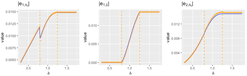
Refer to caption
Figure 2: The value of |e1,θ0||e_{1,\theta_{0}}|, |e1,Σ||e_{1,\Sigma}|, and |e2,θ0||e_{2,\theta_{0}}| as functions of δ\delta. Assume ‖θ0‖=1\|\theta_{0}\|=1, Σ=𝐈p\Sigma=\mathbf{I}_{p}. Blue curve is obtained from Theorem 5 given (θ^0,Σ^)(\widehat{\theta}_{0},\widehat{\Sigma}). Orange points are obtained from simulation. n=1000n=1000, σ2=1\sigma^{2}=1. The two vertical dashed lines in each figure represent δ1\delta_{1} and δ2\delta_{2}.

5.2 Reducing estimation error through additional unlabeled data

Unlabeled data is commonly used in semi-supervised learning, e.g. locally-weighted nearest neighbors algorithm [5]. Besides, in the context of adversarially robust learning, some studies also observed the benefits of using extra unlabeled data [25].

We study the effect of extra unlabeled data on the minimax lower bounds and the upper bounds of our proposed method under different scenarios. With the existence of extra unlabeled data, the minimiax lower bounds become smaller. In addition, these data also help reduce the upper bounds through improving the accuracy of Σ^\widehat{\Sigma}.

If we move one more step from Theorem 1 and 2 and allow the usage of extra unlabeled data, the lower bounds can be reduced:

Theorem 6.

Under the conditions in Theorem 1, if there are extra n1n_{1} samples of unlabeled data, the lower bound becomes Ω⁡((p​σ2/n)∨(p​R2/(n+n1)))\Omega((p\sigma^{2}/n)\vee(pR^{2}/(n+n_{1}))).

Under the conditions in Theorem 2, if there are extra n1n_{1} samples of unlabeled data, the lower bound becomes

Ω⁡(s​σ2​log⁡(p/s)n∨R2​(n+n1)−2​α2​α+1).\Omega\left(s\sigma^{2}\frac{\log(p/s)}{n}\vee R^{2}(n+n_{1})^{-\frac{2\alpha}{2\alpha+1}}\right).

In terms of the upper bounds, since the estimation of Σ^\widehat{\Sigma} is only related to 𝐱{\bf x}, one can directly utilize these extra unlabeled data into the two-stage framework. The following result is extended from Theorem 4:

Corollary 3.

Under the conditions in Corollary 1, if there are extra n1n_{1} samples of unlabeled data, the upper bound becomes O⁡((p​σ2/n)∨(p​R2/(n+n1)))O((p\sigma^{2}/n)\vee(pR^{2}/(n+n_{1}))).

Under the conditions in Corollary 2, if there are extra n1n_{1} samples of unlabeled data, the bound becomes

O⁡(s​σ2​log⁡(p/s)n∨R2​(n+n1)−2​α2​α+1).O\left(s\sigma^{2}\frac{\log(p/s)}{n}\vee R^{2}(n+n_{1})^{-\frac{2\alpha}{2\alpha+1}}\right).

To summarize, as both lower bounds and upper bounds are reduced, it is essential and effective to utilize extra unlabeled data for adversarially robust learning. A numerical illustration is also given in the next section of experiments.

6 Numerical Experiments

In numerical experiments, we consider Example 2, and adopt LASSO/sparse estimators in the first stage to improve adversarial robustness.

We consider the following specifications of (θ0,Σ)(\theta_{0},\Sigma): θ0\theta_{0} is randomly generated from ∂B⁡(0,1)\partial B(0,1), the sphere of a ℒ2\mathcal{L}_{2} ball; the diagonal elements in Σ\Sigma are Σi​i=2​r+|τi|\Sigma_{ii}=2r+|\tau_{i}|, where τi\tau_{i}’s follow i.i.d. standard Gaussian, and the other elements in Σ\Sigma are rr. Under this design of Σ\Sigma, coordinates of 𝐱{\bf x} are correlated with each other, and the smallest and largest eigenvalues are within a reasonable range as pp increases. Each experiment was repeated 500 times with σ2=1\sigma^{2}=1. Define Σ^=𝐗⊤​𝐗/n\widehat{\Sigma}={\bf X}^{\top}{\bf X}/n for non-sparse Σ\Sigma.

Empirical coverage when pp is fixed.

As mentioned in Example 2, n​(θ^−θ∗)\sqrt{n}(\widehat{\theta}-\theta^{*}) asymptotically converges to a zero-mean Gaussian when δ<δ2\delta<\delta_{2}. We use empirical coverage to verify this statement. In this experiment, θ0=(1,2)⊤\theta_{0}=(1,2)^{\top} and Σi​i=i\Sigma_{ii}=i for i=1,2i=1,2 with Σ12=0.5\Sigma_{12}=0.5. For each δ\delta, we repeat the experiment of estimating θ∗\theta^{*} for 1000 times using 1000 samples, and calculate the 95% empirical coverage for θ1∗\theta^{*}_{1} and θ2∗\theta^{*}_{2}. In Figure 3, when δ<1.9\delta<1.9, the magnitude of θi∗\theta^{*}_{i}’s are away from zero, and the empirical coverage for both θi∗\theta^{*}_{i}’s are close to 0.95. When δ>1.9\delta>1.9, θi∗\theta^{*}_{i}’s are almost zero, and the corresponding empirical coverages are a little bit away from 0.95.

Figure 3: Value of θi∗\theta^{*}_{i} and the 95% Empirical Coverage. Blue line: θi∗/θ0​i\theta^{*}_{i}/\theta_{0i}. Orange line: 95% Empirical Coverage. Purple dased line: 0.95. The 95% coverage for both θ1∗\theta^{*}_{1} and θ2∗\theta^{*}_{2} are close to 0.95 when δ<1.9\delta<1.9.

Sparse coefficients.

In this experiment, we verify that LASSO helps obtaining better adversarially robust estimate. We take p=50p=50, n=300n=300, and assume Σ\Sigma is known. Cross validation was applied to choose the penalty that minimizes the (standard) prediction risk. Such a task was implemented by function cv.glmnet in library glmnet in R.

We consider both lower-dimensional dense (Table 1) case with (p,n)=(50,300)(p,n)=(50,300) and high-dimensional sparse scenario with (p,n)=(300,200)(p,n)=(300,200). For high-dimensional sparse model, to make it clear on the difference between θ^O​L​S\widehat{\theta}_{OLS} and θ^L​A​S​S​O\widehat{\theta}_{LASSO}, we present the results given Σ\Sigma is known/unknown. In the dense coefficient model, although we can select a λ\lambda such that the LASSO estimator leads to a smaller standard risk than OLS estimator, its corresponding adversarial risk gets worse with an increasing δ\delta. For the sparse model, for all choices of δ\delta, LASSO has a smaller adversarial risk than OLS. The results for unknown Σ\Sigma are similar with the case when Σ\Sigma is known in the sense that the performance of LASSO is also better than OLS.

In addition, R0​(θ^L​A​S​S​O,δ)R_{0}(\widehat{\theta}_{LASSO},\delta) is always smaller when Σ\Sigma is known than when Σ\Sigma is unknown. This also verifies that unlabeled data helps improve the adversarial robustness (the comparison is not applicable to R0​(θ^O​L​S,δ)R_{0}(\widehat{\theta}_{OLS},\delta) since θ^O​L​S\widehat{\theta}_{OLS} is not consistent).

Table 1: Comparison between OLS and LASSO for dense θ0\theta_{0} with known Σ\Sigma. p=50p=50, n=300n=300, r=0.1r=0.1, σ2=1\sigma^{2}=1. Σ\Sigma is known. Standard deviation is provided for R0​(θ∗,δ)−R0​(θ^O​L​S,δ)R_{0}(\theta^{*},\delta)-R_{0}(\widehat{\theta}_{OLS},\delta) and R0​(θ∗,δ)−R0​(θ^L​A​S​S​O,δ)R_{0}(\theta^{*},\delta)-R_{0}(\widehat{\theta}_{LASSO},\delta).
δ\delta R0​(θ∗,δ)R_{0}(\theta^{*},\delta) R0​(θ^O​L​S,δ)R_{0}(\widehat{\theta}_{OLS},\delta) R0​(θ^L​A​S​S​O,δ)R_{0}(\widehat{\theta}_{LASSO},\delta) R0​(θ0,δ)R_{0}(\theta_{0},\delta) R0​(0,δ)R_{0}(0,\delta)
0.5 0.2489 0.8545(0.1413) 0.633(0.0795) 0.25 0.9997
0.8 0.5847 0.8436(0.0867) 0.8516(0.0858) 0.64 0.9997
0.9 0.6862 0.8715(0.65) 0.8888(0.0762) 0.81 0.9997
Table 2: Comparison between OLS and LASSO for sparse θ0\theta_{0} . The first 10 elements of θ0\theta_{0} are 1/101/\sqrt{10}. p=300p=300, n=200n=200, r=0.1r=0.1, σ2=1\sigma^{2}=1.
Σ\Sigma δ\delta R0​(θ∗,δ)R_{0}(\theta^{*},\delta) R0​(θ^O​L​S,δ)R_{0}(\widehat{\theta}_{OLS},\delta) R0​(θ^L​A​S​S​O,δ)R_{0}(\widehat{\theta}_{LASSO},\delta) R0​(θ0,δ)R_{0}(\theta_{0},\delta) R0​(0,δ)R_{0}(0,\delta)
known 0.5 0.25 6.1134(1.0171) 0.7486(0.1200) 0.25 1.8943
1 0.7847 2.7114(0.4124) 0.9941(0.0752) 1 1.8943
2 1.3088 1.4912(0.0431) 1.3684(0.0453) 4 1.8943
3 1.6088 1.7522(0.0641) 1.6435(0.1033) 9 1.8943
unknown 0.5 0.25 2.3533(0.2551) 0.8212(0.0984) 0.25 1.8943
1 0.7847 1.5830(0.1368) 1.1414(0.0732) 1 1.8943
2 1.3088 1.5023(0.0341) 1.4716(0.0358) 4 1.8943
3 1.6088 1.7040(0.0250) 1.6930(0.0494) 9 1.8943
Table 3: Comparison between Σ^\widehat{\Sigma} and Σ^s​p​a​r​s​e\widehat{\Sigma}_{sparse}. p=300p=300, n=200n=200, σ2=1\sigma^{2}=1. θ0\theta_{0} is known. Σ^s​p​a​r​s​e\widehat{\Sigma}_{sparse} performs slightly better when Σ\Sigma is sparse.
δ=2\delta=2 R0​(θ∗,δ)R_{0}(\theta^{*},\delta) R0​(θΣ^∗,δ)R_{0}(\theta^{*}_{\widehat{\Sigma}},\delta) R0​(θΣ^s​p​a​r​s​e∗,δ)R_{0}(\theta^{*}_{\widehat{\Sigma}_{sparse}},\delta) R0​(θ0,δ)R_{0}(\theta_{0},\delta)
Dense 1.8865 2.0576(0.1841) 4.8769(0.1044) 4.0000
Sparse 2.9807 3.0652(0.0279) 3.0293(0.0279) 4.0000

Sparse matrix.

We use sparse matrix estimator to verify that it helps enhancing adversarial robustness. To generate sparse matrix, we consider Σ\Sigma such that Σi​i=1\Sigma_{ii}=1, and Σi​j=r​|i−j|−α−1\Sigma_{ij}=r|i-j|^{-\alpha-1} when j≠ij\neq i, where r=0.6r=0.6 and α=0.2\alpha=0.2. This choice of (r,α)(r,\alpha) ensures that all eigenvalues of Σ\Sigma are positive. We take p=300p=300, n=200n=200 so that the difference between Σ^\widehat{\Sigma} and Σ^s​p​a​r​s​e\widehat{\Sigma}_{sparse} is obvious. The attack level δ\delta is set to be 2 in this comparison. For simplicity, we assume θ0\theta_{0} is known in the comparison of matrix estimators. The sparse covariance estimator Σ^s​p​a​r​s​e\widehat{\Sigma}_{sparse} was obtained based on the method in [4]. In Table 3, the adversarial excess risk is reduced from 0.0845 (R0​(θΣ^∗,δ)−R0​(θ∗,δ)R_{0}(\theta^{*}_{\widehat{\Sigma}},\delta)-R_{0}(\theta^{*},\delta)) to 0.0486 (R0​(θΣ^s​p​a​r​s​e∗,δ)−R0​(θ∗,δ)R_{0}(\theta^{*}_{\widehat{\Sigma}_{sparse}},\delta)-R_{0}(\theta^{*},\delta)), which shows the effectiveness of Σ^s​p​a​r​s​e\widehat{\Sigma}_{sparse}. In addition to sparse matrix, we also consider dense covariance matrix generated in the same way as previous experiments by taking r=0.6r=0.6. When the true martix is dense, using sparse estimate is not appropriate, thus the corresponding adversarial risk is much higher.

7 Conclusions and Future Directions

In this paper, we figure out the minimax lower bound of estimation error of adversarially robust model in linear regression setup, which indicates the it is important to incorporate model information in adversarially robust learning. In addition, we propose a two-stage adversarially robust learning method based on an explicit relation between adversarially robust estimator and standard estimator. The proposed two-stage estimator can encode model information (e.g. sparsity) into standard estimators, through which the robustness of adversarially robust estimator could be improved and reach minimax optimal convergence rate. Our investigation in the generalization error also verifies that adversarial robustness hurts generalization.

One future direction is to relax the distributional assumption on (𝐱,y)({\bf x},y), say 𝐱{\bf x} follows non-Gaussian distribution. Although there is a wide range of data may follow Gaussian assumption, e.g. abalone data and other biological data, many other data may not follow Gaussian, e.g. image data. The constant c0c_{0} in our framework currently depends on the Gaussian assumption, and there is potential to relax it. Another one is concerned with sparse adversarially robust learning, say sparse θ^\widehat{\theta}, which could be useful in both compressing and robustifying deep neural networks [11]. The first step is to understand how the sparsity of θ0\theta_{0} (together with other model assumptions) implies that of θ∗\theta^{*}, which in turn determines the sparsity of θ^\widehat{\theta}. An example can be found in [1] for linear sparse coding model. However, more careful studies would be needed in the future.

References

  • [1] Zeyuan Allen-Zhu and Yuanzhi Li. Feature purification: How adversarial training performs robust deep learning. arXiv preprint arXiv:2005.10190, 2020.
  • [2] Mikhail Belkin, Daniel Hsu, and Ji Xu. Two models of double descent for weak features. CoRR, abs/1903.07571, 2019.
  • [3] Peter J Bickel, Ya’acov Ritov, and Alexandre B Tsybakov. Simultaneous analysis of lasso and dantzig selector. The Annals of Statistics, 37(4):1705–1732, 2009.
  • [4] T Tony Cai, Cun-Hui Zhang, and Harrison H Zhou. Optimal rates of convergence for covariance matrix estimation. The Annals of Statistics, 38(4):2118–2144, 2010.
  • [5] Timothy I Cannings, Thomas B Berrett, Richard J Samworth, et al. Local nearest neighbour classification with applications to semi-supervised learning. Annals of Statistics, 48(3):1789–1814, 2020.
  • [6] Yair Carmon, Aditi Raghunathan, Ludwig Schmidt, John C Duchi, and Percy S Liang. Unlabeled data improves adversarial robustness. In Advances in Neural Information Processing Systems, pages 11190–11201, 2019.
  • [7] Chen Dan, Yuting Wei, and Pradeep Ravikumar. Sharp statistical guarantees for adversarially robust gaussian classification. volume abs/2006.16384, 2020.
  • [8] Lee H Dicker et al. Ridge regression and asymptotic minimax estimation over spheres of growing dimension. Bernoulli, 22(1):1–37, 2016.
  • [9] Christian Etmann, Sebastian Lunz, Peter Maass, and Carola Schönlieb. On the connection between adversarial robustness and saliency map interpretability. In Proceedings of the 36th International Conference on Machine Learning, volume 97 of Proceedings of Machine Learning Research, pages 1823–1832. PMLR, 2019.
  • [10] Ian J. Goodfellow, Jonathon Shlens, and Christian Szegedy. Explaining and harnessing adversarial examples. In 3rd International Conference on Learning Representations, 2015.
  • [11] Yiwen Guo, Chao Zhang, Changshui Zhang, and Yurong Chen. Sparse dnns with improved adversarial robustness. In Advances in neural information processing systems, pages 242–251, 2018.
  • [12] Xuming He and Qi-Man Shao. A general bahadur representation of m-estimators and its application to linear regression with nonstochastic designs. The Annals of Statistics, 24(6):2608–2630, 1996.
  • [13] Daniel Hsu, Sham M Kakade, and Tong Zhang. Random design analysis of ridge regression. In Conference on Learning Theory, pages 9–1, 2012.
  • [14] Ching-Kang Ing and Tze Leung Lai. A stepwise regression method and consistent model selection for high-dimensional sparse linear models. Statistica Sinica, 21(4):1473–1513, 2011.
  • [15] Adel Javanmard, Mahdi Soltanolkotabi, and Hamed Hassani. Precise tradeoffs in adversarial training for linear regression. CoRR, abs/2002.10477, 2020.
  • [16] X Jessie Jeng, Huimin Peng, and Wenbin Lu. Post-lasso inference for high-dimensional regression. CoRR, abs/1806.06304, 2018.
  • [17] Alexey Kurakin, Ian J. Goodfellow, and Samy Bengio. Adversarial machine learning at scale. In 5th International Conference on Learning Representations. OpenReview.net, 2017.
  • [18] Shiqing Ma, Yingqi Liu, Guanhong Tao, Wen-Chuan Lee, and Xiangyu Zhang. Nic: Detecting adversarial samples with neural network invariant checking. In Network and Distributed System Security Symposium, 2019.
  • [19] Song Mei, Yu Bai, and Andrea Montanari. The landscape of empirical risk for nonconvex losses. The Annals of Statistics, 46(6A):2747–2774, 2018.
  • [20] Jaouad Mourtada. Exact minimax risk for linear least squares, and the lower tail of sample covariance matrices. arXiv preprint arXiv:1912.10754, 2019.
  • [21] Amir Najafi, Shin-ichi Maeda, Masanori Koyama, and Takeru Miyato. Robustness to adversarial perturbations in learning from incomplete data. In Advances in Neural Information Processing Systems, pages 5542–5552, 2019.
  • [22] Steven W. Nydick. The wishart and inverse wishart distributions. 2012.
  • [23] Nicolas Papernot, Patrick McDaniel, Ian Goodfellow, Somesh Jha, Z Berkay Celik, and Ananthram Swami. Practical black-box attacks against machine learning. In Proceedings of the 2017 ACM on Asia Conference on Computer and Communications Security, pages 506–519. ACM, 2017.
  • [24] Nicolas Papernot, Patrick McDaniel, Ananthram Swami, and Richard Harang. Crafting adversarial input sequences for recurrent neural networks. In Military Communications Conference, MILCOM 2016-2016 IEEE, pages 49–54. IEEE, 2016.
  • [25] Aditi Raghunathan, Sang Michael Xie, Fanny Yang, John C. Duchi, and Percy Liang. Adversarial training can hurt generalization. CoRR, abs/1906.06032, 2019.
  • [26] Garvesh Raskutti, Martin J Wainwright, and Bin Yu. Minimax rates of estimation for high-dimensional linear regression over lq-balls. IEEE transactions on information theory, 57(10):6976–6994, 2011.
  • [27] Ludwig Schmidt, Shibani Santurkar, Dimitris Tsipras, Kunal Talwar, and Aleksander Madry. Adversarially robust generalization requires more data. In Advances in Neural Information Processing Systems, pages 5014–5026, 2018.
  • [28] Uri Shaham, Yutaro Yamada, and Sahand Negahban. Understanding adversarial training: Increasing local stability of neural nets through robust optimization. CoRR, abs/1511.05432, 2015.
  • [29] Aman Sinha, Hongseok Namkoong, and John Duchi. Certifiable distributional robustness with principled adversarial training. In International Conference on Learning Representations, 2018.
  • [30] Guanhong Tao, Shiqing Ma, Yingqi Liu, and Xiangyu Zhang. Attacks meet interpretability: Attribute-steered detection of adversarial samples. In Advances in Neural Information Processing Systems, pages 7717–7728, 2018.
  • [31] Nicolas Verzelen. High-dimensional gaussian model selection on a gaussian design. In Annales de l’IHP Probabilités et statistiques, volume 46, pages 480–524, 2010.
  • [32] Yisen Wang, Xingjun Ma, James Bailey, Jinfeng Yi, Bowen Zhou, and Quanquan Gu. On the convergence and robustness of adversarial training. In Proceedings of the 35th International Conference on Machine Learning, volume 97 of Proceedings of Machine Learning Research, pages 6586–6595. PMLR, 2019.
  • [33] Yue Xing, Qifan Song, and Guang Cheng. On the generalization properties of adversarial training. arXiv preprint arXiv:2008.06631, 2020.
  • [34] Huan Xu, Constantine Caramanis, and Shie Mannor. Robust regression and lasso. In Advances in neural information processing systems, pages 1801–1808, 2009.
  • [35] Huan Xu, Constantine Caramanis, and Shie Mannor. Robustness and regularization of support vector machines. Journal of machine learning research, 10(7), 2009.
  • [36] Huan Xu and Shie Mannor. Robustness and generalization. Machine learning, 86(3):391–423, 2012.
  • [37] Weilin Xu, David Evans, and Yanjun Qi. Feature squeezing: Detecting adversarial examples in deep neural networks. In 25th Annual Network and Distributed System Security Symposium. The Internet Society, 2018.
  • [38] Fei Ye and Cun-Hui Zhang. Rate minimaxity of the lasso and dantzig selector for the lq loss in lr balls. The Journal of Machine Learning Research, 11:3519–3540, 2010.
  • [39] Dong Yin, Kannan Ramchandran, and Peter L. Bartlett. Rademacher complexity for adversarially robust generalization. In Proceedings of the 36th International Conference on Machine Learning, volume 97 of Proceedings of Machine Learning Research, pages 7085–7094. PMLR, 2019.
  • [40] Runtian Zhai, Tianle Cai, Di He, Chen Dan, Kun He, John E. Hopcroft, and Liwei Wang. Adversarially robust generalization just requires more unlabeled data. CoRR, abs/1906.00555, 2019.
  • [41] Guoming Zhang, Chen Yan, Xiaoyu Ji, Tianchen Zhang, Taimin Zhang, and Wenyuan Xu. Dolphinattack: Inaudible voice commands. In Proceedings of the 2017 ACM SIGSAC Conference on Computer and Communications Security, pages 103–117. ACM, 2017.
  • [42] Hongyang Zhang, Yaodong Yu, Jiantao Jiao, Eric P. Xing, Laurent El Ghaoui, and Michael I. Jordan. Theoretically principled trade-off between robustness and accuracy. In Proceedings of the 36th International Conference on Machine Learning, volume 97 of Proceedings of Machine Learning Research, pages 7472–7482. PMLR, 2019.

Appendix A More theoretical results

This section provides some supplementary theorems.

A.1 Results regarding to prediction risk (an analog of Theorem 3)

For consistent estimates (θ^0,Σ^,σ^2)(\widehat{\theta}_{0},\widehat{\Sigma},\widehat{\sigma}^{2}), with probability tending to 1, we have

supδ≥0|R⁡(θ∗​(δ),δ)−R⁡(θ~​(δ),δ)|\displaystyle\sup\limits_{\delta\geq 0}\left|R(\theta^{*}(\delta),\delta)-R(\widetilde{\theta}(\delta),\delta)\right| =\displaystyle= O⁡(‖θ^0−θ0‖​‖θ0‖)+O⁡(‖θ0‖2​‖Σ^−Σ‖)\displaystyle O\left(\|\widehat{\theta}_{0}-\theta_{0}\|\|\theta_{0}\|\right)+O\left(\|\theta_{0}\|^{2}\sqrt{\|\widehat{\Sigma}-\Sigma\|}\right)
+O⁡(σ^2−σ2)+O⁡(‖θ0‖​(σ^−σ)).\displaystyle+O\left(\widehat{\sigma}^{2}-\sigma^{2}\right)+O\left(\|\theta_{0}\|(\widehat{\sigma}-\sigma)\right).

A.2 Definitions in Theorem 4

𝐌1​(θ∗,θ0,Σ)\displaystyle\mathbf{M}_{1}(\theta^{*},\theta_{0},\Sigma) =\displaystyle= 𝐇​(θ∗,θ0,Σ)−1​𝐌​(θ∗,θ0,Σ),\displaystyle\mathbf{H}(\theta^{*},\theta_{0},\Sigma)^{-1}\mathbf{M}(\theta^{*},\theta_{0},\Sigma),
𝐌2​(θ∗,θ0,Σ)\displaystyle\mathbf{M}_{2}(\theta^{*},\theta_{0},\Sigma) =\displaystyle= −δ​c0​𝐇​(θ∗,θ0,Σ)−1​(Σ⁡(θ∗−θ0)2​‖θ∗−θ0‖Σ​‖θ∗‖−‖θ∗‖​θ∗2​‖θ∗−θ0‖Σ3),\displaystyle-\delta c_{0}\mathbf{H}(\theta^{*},\theta_{0},\Sigma)^{-1}\left(\frac{\Sigma(\theta^{*}-\theta_{0})}{2\|\theta^{*}-\theta_{0}\|_{\Sigma}\|\theta^{*}\|}-\frac{\|\theta^{*}\|\theta^{*}}{2\|\theta^{*}-\theta_{0}\|_{\Sigma}^{3}}\right),
𝐌3​(θ∗,θ0,Σ)\displaystyle\mathbf{M}_{3}(\theta^{*},\theta_{0},\Sigma) =\displaystyle= −(1+δ​c0​A​(θ∗,θ0,Σ)),\displaystyle-(1+\delta c_{0}A(\theta^{*},\theta_{0},\Sigma)),
𝐌⁡(θ∗,θ0,Σ)\displaystyle\mathbf{M}(\theta^{*},\theta_{0},\Sigma) =\displaystyle= Σ+δ​c0​A​(θ∗,θ0,Σ)​Σ+δ​c0​A​(θ∗,θ0,Σ)‖θ∗−θ0‖Σ2​Σ​(θ∗−θ0)​(θ∗−θ0)⊤​Σ\displaystyle\Sigma+\delta c_{0}A(\theta^{*},\theta_{0},\Sigma)\Sigma+\frac{\delta c_{0}A(\theta^{*},\theta_{0},\Sigma)}{\|\theta^{*}-\theta_{0}\|^{2}_{\Sigma}}\Sigma(\theta^{*}-\theta_{0})(\theta^{*}-\theta_{0})^{\top}\Sigma
+δ​c0A⁡(θ∗,θ0,Σ)​‖θ∗‖22​θ∗​(θ∗)⊤,\displaystyle+\delta\frac{c_{0}}{A(\theta^{*},\theta_{0},\Sigma)\|\theta^{*}\|^{2}_{2}}\theta^{*}(\theta^{*})^{\top},

where A⁡(θ∗,θ0,Σ)=‖θ∗‖/‖θ∗−θ0‖ΣA(\theta^{*},\theta_{0},\Sigma)=\|\theta^{*}\|/\|\theta^{*}-\theta_{0}\|_{\Sigma}. The matrix 𝐇⁡(θ∗,θ0,Σ)\mathbf{H}(\theta^{*},\theta_{0},\Sigma) is the Hessian matrix of R0R_{0}.

Appendix B Proofs in Section 2

There are two parts of Proposition 1: the statement about Hessian, and the optimal solution θ∗\theta^{*}. We prove them separately.

B.1 Positive definite Hessian

Proof of Proposition 1 for Positive Definite Hessian.

Expand the adversarial risk at 𝐱{\bf x} as

max‖x∗−x‖≤δ​[((x∗)⊤​θ−𝐱⊤​θ0)2]\displaystyle\underset{\|x^{*}-x\|\leq\delta}{\max}\left[(\mathbf{(}x^{*})^{\top}\theta-\mathbf{x}^{\top}\theta_{0})^{2}\right] =\displaystyle= max‖x∗−x‖≤δ​[(𝐱∗−𝐱)⊤​θ+𝐱⊤​(θ−θ0)]2\displaystyle\underset{\|x^{*}-x\|\leq\delta}{\max}\left[(\mathbf{x}^{*}-\mathbf{x})^{\top}\theta+\mathbf{x}^{\top}(\theta-\theta_{0})\right]^{2}
=\displaystyle= (δ​‖θ‖+|𝐱⊤​(θ−θ0)|)2.\displaystyle\left(\delta\|\theta\|+|\mathbf{x}^{\top}(\theta-\theta_{0})|\right)^{2}.

Since 𝐱{\bf x} follows Gaussian, for any fixed θ−θ0\theta-\theta_{0}, 𝐱⊤​(θ−θ0){\bf x}^{\top}(\theta-\theta_{0}) follows Gaussian as well. Let Z=𝐱⊤​(θ−θ0).Z=\mathbf{x}^{\top}(\theta-\theta_{0}). Note that 𝐱∼N⁡(𝟎,Σ),{\bf x}\sim N(\mathbf{0},\Sigma), we have Z∼N⁡(0,‖θ−θ0‖Σ2)Z\sim N(0,\|\theta-\theta_{0}\|^{2}_{\Sigma}) and

R0​(θ,δ)\displaystyle R_{0}(\theta,\delta) =\displaystyle= 𝔼Z​(|Z|+δ​‖θ‖)2\displaystyle{\mathbb{E}}_{Z}(|Z|+\delta\|\theta\|)^{2}
=\displaystyle= ‖θ−θ0‖Σ2+2​δ​c0​‖θ‖​‖θ−θ0‖Σ+δ2​‖θ‖22.\displaystyle\|\theta-\theta_{0}\|^{2}_{\Sigma}+2\delta c_{0}\|\theta\|\|\theta-\theta_{0}\|_{\Sigma}+\delta^{2}\|\theta\|^{2}_{2}.

Taking the gradient of R0​(θ,δ)R_{0}(\theta,\delta) with respect to θ\theta yields

∇θR0​(θ,δ)\displaystyle\nabla_{\theta}R_{0}(\theta,\delta) =\displaystyle= 2​[Σ⁡(θ−θ0)+δ​c0​‖θ−θ0‖Σ‖θ‖​θ+δ​c0​‖θ‖‖θ−θ0‖Σ​Σ​(θ−θ0)+δ2​θ]\displaystyle 2\left[\Sigma(\theta-\theta_{0})+\delta c_{0}\frac{\|\theta-\theta_{0}\|_{\Sigma}}{\|\theta\|}\theta+\delta c_{0}\frac{\|\theta\|}{\|\theta-\theta_{0}\|_{\Sigma}}\Sigma(\theta-\theta_{0})+\delta^{2}\theta\right]
=\displaystyle= 2​[(𝐈p+δ​c0​‖θ‖‖θ−θ0‖Σ)​Σ​(θ−θ0)+(δ​c0​‖θ−θ0‖Σ‖θ‖+δ2)​θ].\displaystyle 2\left[\left(\mathbf{I}_{p}+\delta c_{0}\frac{\|\theta\|}{\|\theta-\theta_{0}\|_{\Sigma}}\right)\Sigma(\theta-\theta_{0})+\left(\delta c_{0}\frac{\|\theta-\theta_{0}\|_{\Sigma}}{\|\theta\|}+\delta^{2}\right)\theta\right].

Denote A=‖θ‖/‖θ−θ0‖ΣA=\|\theta\|/\|\theta-\theta_{0}\|_{\Sigma}, then ∂2R02​∂θ2\frac{\partial^{2}R_{0}}{2\partial\theta^{2}} becomes

𝐇:=∂2R02​∂θ2=Σ+δ​c0​A​Σ+(δ​c0A+δ2)​𝐈p+δ​c0​Σ​(θ−θ0)​(∂A∂θ)⊤+δ​c0​θ​(∂1/A∂θ)⊤.\displaystyle\mathbf{H}:=\frac{\partial^{2}R_{0}}{2\partial\theta^{2}}=\Sigma+\delta c_{0}A\Sigma+\left(\frac{\delta c_{0}}{A}+\delta^{2}\right)\mathbf{I}_{p}+\delta c_{0}\Sigma(\theta-\theta_{0})\left(\frac{\partial A}{\partial\theta}\right)^{\top}+\delta c_{0}\theta\left(\frac{\partial 1/A}{\partial\theta}\right)^{\top}. (10)

To show that R0R_{0} is convex, it sufficies to show that HH is positive definite.

In 𝐇\mathbf{H}, the two partial derivatives are

∂A∂θ\displaystyle\frac{\partial A}{\partial\theta} =\displaystyle= ∂∂θ​‖θ‖‖θ−θ0‖Σ=θ‖θ‖​‖θ−θ0‖Σ−‖θ‖​Σ​(θ−θ0)‖θ−θ0‖Σ3,\displaystyle\frac{\partial}{\partial\theta}\frac{\|\theta\|}{\|\theta-\theta_{0}\|_{\Sigma}}=\frac{\theta}{\|\theta\|\|\theta-\theta_{0}\|_{\Sigma}}-\frac{\|\theta\|\Sigma(\theta-\theta_{0})}{\|\theta-\theta_{0}\|_{\Sigma}^{3}},

and

∂1/A∂θ=Σ⁡(θ−θ0)‖θ‖​‖θ−θ0‖Σ−‖θ−θ0‖Σ​θ‖θ‖3.\displaystyle\frac{\partial 1/A}{\partial\theta}=\frac{\Sigma(\theta-\theta_{0})}{\|\theta\|\|\theta-\theta_{0}\|_{\Sigma}}-\frac{\|\theta-\theta_{0}\|_{\Sigma}\theta}{\|\theta\|^{3}}.

Thus

Σ⁡(θ−θ0)​(∂A∂θ)⊤\displaystyle\Sigma(\theta-\theta_{0})\left(\frac{\partial A}{\partial\theta}\right)^{\top} =\displaystyle= 1‖θ‖​‖θ−θ0‖Σ​Σ​(θ−θ0)​θ⊤−‖θ‖‖θ−θ0‖Σ3​Σ​(θ−θ0)​(θ−θ0)⊤​Σ,\displaystyle\frac{1}{\|\theta\|\|\theta-\theta_{0}\|_{\Sigma}}\Sigma(\theta-\theta_{0})\theta^{\top}-\frac{\|\theta\|}{\|\theta-\theta_{0}\|_{\Sigma}^{3}}\Sigma(\theta-\theta_{0})(\theta-\theta_{0})^{\top}\Sigma,
=\displaystyle= 1‖θ‖​‖θ−θ0‖Σ​Σ​(θ−θ0)​θ⊤−A‖θ−θ0‖Σ2​Σ​(θ−θ0)​(θ−θ0)⊤​Σ,\displaystyle\frac{1}{\|\theta\|\|\theta-\theta_{0}\|_{\Sigma}}\Sigma(\theta-\theta_{0})\theta^{\top}-\frac{A}{\|\theta-\theta_{0}\|_{\Sigma}^{2}}\Sigma(\theta-\theta_{0})(\theta-\theta_{0})^{\top}\Sigma,
θ​(∂1/A∂θ)⊤\displaystyle\theta\left(\frac{\partial 1/A}{\partial\theta}\right)^{\top} =\displaystyle= 1‖θ‖​‖θ−θ0‖Σ​θ​(θ−θ0)⊤​Σ−‖θ−θ0‖Σ‖θ‖3​θ​θ⊤,\displaystyle\frac{1}{\|\theta\|\|\theta-\theta_{0}\|_{\Sigma}}\theta(\theta-\theta_{0})^{\top}\Sigma-\frac{\|\theta-\theta_{0}\|_{\Sigma}}{\|\theta\|^{3}}\theta\theta^{\top},
=\displaystyle= 1‖θ‖​‖θ−θ0‖Σ​θ​(θ−θ0)⊤​Σ−1A​‖θ‖2​θ​θ⊤.\displaystyle\frac{1}{\|\theta\|\|\theta-\theta_{0}\|_{\Sigma}}\theta(\theta-\theta_{0})^{\top}\Sigma-\frac{1}{A\|\theta\|^{2}}\theta\theta^{\top}.

Then 𝐇\mathbf{H} can be represented as

Σ+δ​c0​A​Σ+(δ​c0A+δ2)​𝐈p+δ​c0​Σ​(θ−θ0)​(∂A∂θ)⊤+δ​c0​θ​(∂1/A∂θ)⊤\displaystyle\Sigma+\delta c_{0}A\Sigma+\left(\frac{\delta c_{0}}{A}+\delta^{2}\right)\mathbf{I}_{p}+\delta c_{0}\Sigma(\theta-\theta_{0})\left(\frac{\partial A}{\partial\theta}\right)^{\top}+\delta c_{0}\theta\left(\frac{\partial 1/A}{\partial\theta}\right)^{\top}
=\displaystyle= (Σ−1‖θ−θ0‖Σ2​Σ​(θ−θ0)​(θ−θ0)⊤​Σ)​A​c0​δ\displaystyle\left(\Sigma-\frac{1}{\|\theta-\theta_{0}\|^{2}_{\Sigma}}\Sigma(\theta-\theta_{0})(\theta-\theta_{0})^{\top}\Sigma\right)Ac_{0}\delta
+(𝐈p−1‖θ‖2​θ​θ⊤)​c0​δA\displaystyle+\left(\mathbf{I}_{p}-\frac{1}{\|\theta\|^{2}}\theta\theta^{\top}\right)\frac{c_{0}\delta}{A}
+(Σ+δ2​𝐈p+δ​c0‖θ‖​‖θ−θ0‖Σ​θ​(θ−θ0)⊤​Σ+δ​c0‖θ‖​‖θ−θ0‖Σ​Σ​(θ−θ0)​θ⊤)\displaystyle+\left(\Sigma+\delta^{2}\mathbf{I}_{p}+\frac{\delta c_{0}}{\|\theta\|\|\theta-\theta_{0}\|_{\Sigma}}\theta(\theta-\theta_{0})^{\top}\Sigma+\frac{\delta c_{0}}{\|\theta\|\|\theta-\theta_{0}\|_{\Sigma}}\Sigma(\theta-\theta_{0})\theta^{\top}\right)
:⁣=\displaystyle:= 𝐌1​A​c0​δ+𝐌2​c0​δA+𝐌3.\displaystyle\mathbf{M}_{1}Ac_{0}\delta+\mathbf{M}_{2}\frac{c_{0}\delta}{A}+\mathbf{M}_{3}.

Since Σ\Sigma is positive definite, for any vector 𝐚≠𝟎,\mathbf{a}\neq\mathbf{0}, and θ≠θ0,θ≠𝟎,\theta\neq\theta_{0},\theta\neq\mathbf{0}, by Cauchy inequality,

𝐚⊤​𝐌1​𝐚\displaystyle\mathbf{a}^{\top}\mathbf{M}_{1}\mathbf{a} =\displaystyle= 𝐚⊤​Σ​𝐚−(𝐚⊤​Σ​(θ−θ0))2.‖θ−θ0‖Σ2≥0,\displaystyle\mathbf{a}^{\top}\Sigma\mathbf{a}-\frac{\left(\mathbf{a}^{\top}\Sigma(\theta-\theta_{0})\right)^{2}.}{\|\theta-\theta_{0}\|_{\Sigma}^{2}}\geq 0,
𝐚⊤​𝐌2​𝐚\displaystyle\mathbf{a}^{\top}\mathbf{M}_{2}\mathbf{a} =\displaystyle= 𝐚⊤​𝐚−(𝐚⊤​θ)2‖θ‖2≥0,\displaystyle\mathbf{a}^{\top}\mathbf{a}-\frac{(\mathbf{a}^{\top}\theta)^{2}}{\|\theta\|^{2}}\geq 0,

which imply 𝐌1\mathbf{M}_{1} and 𝐌2\mathbf{M}_{2} are positive semi-definite.

For 𝐌3\mathbf{M}_{3}, we have

𝐌3\displaystyle\mathbf{M}_{3} =\displaystyle= [δ​𝐈p+c0‖θ‖​‖θ−θ0‖Σ​Σ​(θ−θ0)​θ⊤]​[δ​𝐈p+c0‖θ‖​‖θ−θ0‖Σ​Σ​(θ−θ0)​θ⊤]⊤\displaystyle\left[\delta\mathbf{I}_{p}+\frac{c_{0}}{\|\theta\|\|\theta-\theta_{0}\|_{\Sigma}}\Sigma(\theta-\theta_{0})\theta^{\top}\right]\left[\delta\mathbf{I}_{p}+\frac{c_{0}}{\|\theta\|\|\theta-\theta_{0}\|_{\Sigma}}\Sigma(\theta-\theta_{0})\theta^{\top}\right]^{\top}
+Σ−c02‖θ−θ0‖Σ2​Σ​(θ−θ0)​(θ−θ0)⊤​Σ.\displaystyle+\Sigma-\frac{c_{0}^{2}}{\|\theta-\theta_{0}\|_{\Sigma}^{2}}\Sigma(\theta-\theta_{0})(\theta-\theta_{0})^{\top}\Sigma.

Since c0=2/π<1,c_{0}=\sqrt{2/\pi}<1, for any vector 𝐚≠𝟎,\mathbf{a}\neq\mathbf{0}, and θ≠θ0,θ≠𝟎,\theta\neq\theta_{0},\theta\neq\mathbf{0},

𝐚⊤​(Σ−c02‖θ−θ0‖Σ2​Σ​(θ−θ0)​(θ−θ0)⊤​Σ)​𝐚\displaystyle\mathbf{a}^{\top}\left(\Sigma-\frac{c_{0}^{2}}{\|\theta-\theta_{0}\|_{\Sigma}^{2}}\Sigma(\theta-\theta_{0})(\theta-\theta_{0})^{\top}\Sigma\right)\mathbf{a} >\displaystyle> 𝐚⊤​𝐌1​𝐚≥0.\displaystyle\mathbf{a}^{\top}\mathbf{M}_{1}\mathbf{a}\geq 0.

∎

B.2 Optimal solution

Proof of Proposition 1 for θ∗\theta^{*}.

We first consider the case where Σ\Sigma is a diagonal matrix. Recall that the gradient of R0​(θ,δ)R_{0}(\theta,\delta) is

∇θR0​(θ,δ)\displaystyle\nabla_{\theta}R_{0}(\theta,\delta) =\displaystyle= 2​[Σ⁡(θ−θ0)+δ​c0​‖θ−θ0‖Σ‖θ‖​θ+δ​c0​‖θ‖‖θ−θ0‖Σ​Σ​(θ−θ0)+δ2​θ]\displaystyle 2\left[\Sigma(\theta-\theta_{0})+\delta c_{0}\frac{\|\theta-\theta_{0}\|_{\Sigma}}{\|\theta\|}\theta+\delta c_{0}\frac{\|\theta\|}{\|\theta-\theta_{0}\|_{\Sigma}}\Sigma(\theta-\theta_{0})+\delta^{2}\theta\right]
=\displaystyle= 2​[(𝐈p+δ​c0​‖θ‖‖θ−θ0‖Σ)​Σ​(θ−θ0)+(δ​c0​‖θ−θ0‖Σ‖θ‖+δ2)​θ].\displaystyle 2\left[\left(\mathbf{I}_{p}+\delta c_{0}\frac{\|\theta\|}{\|\theta-\theta_{0}\|_{\Sigma}}\right)\Sigma(\theta-\theta_{0})+\left(\delta c_{0}\frac{\|\theta-\theta_{0}\|_{\Sigma}}{\|\theta\|}+\delta^{2}\right)\theta\right].

Note the gradient ∇θR0​(θ,δ)\nabla_{\theta}R_{0}(\theta,\delta) is well-defined in ℝp/{𝟎,θ0}\mathbb{R}^{p}/\{\mathbf{0},\theta_{0}\} and R0​(θ,δ)→+∞R_{0}(\theta,\delta)\to+\infty as ‖θ‖→+∞.\|\theta\|\to+\infty. Thus, the global minimizer θ∗\theta^{*} of R0​(θ,δ)R_{0}(\theta,\delta) should only be 𝟎,θ0\mathbf{0},\theta_{0} or the stationary point of R0​(θ,δ).R_{0}(\theta,\delta). Note if ∇θR0​(θ,δ)=𝟎,\nabla_{\theta}R_{0}(\theta,\delta)=\bf 0, we have η​Σ​(θ−θ0)=−θ\eta\Sigma(\theta-\theta_{0})=-\theta for some η>0,\eta>0, or equivalently,

θη=(η​Σ+𝐈p)−1​η​Σ​θ0=[𝐈p−(η​Σ+𝐈p)−1]​θ0.\displaystyle\theta_{\eta}=(\eta\Sigma+\mathbf{I}_{p})^{-1}\eta\Sigma\theta_{0}=\left[\mathbf{I}_{p}-(\eta\Sigma+\mathbf{I}_{p})^{-1}\right]\theta_{0}.

Since when η→0,\eta\to 0, θη→𝟎\theta_{\eta}\to\mathbf{0} and when η→+∞,\eta\to+\infty, θη→θ0,\theta_{\eta}\to\theta_{0}, the global minimizer of R0​(θ,δ)R_{0}(\theta,\delta) should has the form as [I−(η​Σ+𝐈p)−1]​θ0\left[I-(\eta\Sigma+\mathbf{I}_{p})^{-1}\right]\theta_{0} for some η∈[0,∞].\eta\in[0,\infty]. Define

r⁡(η)\displaystyle r(\eta) =\displaystyle= R0​(θη,δ),\displaystyle R_{0}(\theta_{\eta},\delta), (11)
θη\displaystyle\theta_{\eta} =\displaystyle= (𝐈p−(η​Σ+𝐈p)−1)​θ0,\displaystyle(\mathbf{I}_{p}-(\eta\Sigma+\mathbf{I}_{p})^{-1})\theta_{0}, (12)
H⁡(η)\displaystyle H(\eta) =\displaystyle= θ0⊤​(Ση​Σ+𝐈p)2​θ0θ0⊤​Σ(η​Σ+𝐈p)2​θ0,\displaystyle\frac{\sqrt{\theta^{\top}_{0}(\frac{\Sigma}{\eta\Sigma+\mathbf{I}_{p}})^{2}\theta_{0}}}{\sqrt{\theta^{\top}_{0}\frac{\Sigma}{(\eta\Sigma+\mathbf{I}_{p})^{2}}\theta_{0}}}, (13)
g⁡(η)\displaystyle g(\eta) =\displaystyle= 1−δ​c0H⁡(η)+η⁡(δ​c0​H​(η)−δ2).\displaystyle 1-\frac{\delta c_{0}}{H(\eta)}+\eta(\delta c_{0}H(\eta)-\delta^{2}). (14)

We have

r′​(η)=∂∂η​R0​(θη,δ)\displaystyle r^{\prime}(\eta)=\frac{\partial}{\partial\eta}R_{0}(\theta_{\eta},\delta) =\displaystyle= (∇θR0​(θη))⊤​∂∂η​θη\displaystyle(\nabla_{\theta}R_{0}(\theta_{\eta}))^{\top}\frac{\partial}{\partial\eta}\theta_{\eta} (15)
=\displaystyle= −2​g​(η)​(θ−θ0)⊤​Σ​(η​Σ+𝐈p)−1​Σ​(θ−θ0).\displaystyle-2g(\eta)(\theta-\theta_{0})^{\top}\Sigma(\eta\Sigma+\mathbf{I}_{p})^{-1}\Sigma(\theta-\theta_{0}).

By Lemma 1 below, if δ≤δ1,\delta\leq\delta_{1}, g⁡(η)>0.g(\eta)>0. Thus, r⁡(η)r(\eta) is decreasing and the global minimizer of R0​(θ,δ)R_{0}(\theta,\delta) is θη=+∞=θ0\theta_{\eta=+\infty}=\theta_{0}. If δ≥δ2,\delta\geq\delta_{2}, g⁡(η)<0.g(\eta)<0. Thus, r⁡(η)r(\eta) is increasing and the global minimizer of R0​(θ,δ)R_{0}(\theta,\delta) is θη=0=𝟎\theta_{\eta=0}=\mathbf{0}. If δ1<δ<δ2,\delta_{1}<\delta<\delta_{2}, there exists a unique positive number η∗\eta^{*} (as denoted as η∗​(δ)\eta^{*}(\delta)) such that g⁡(η∗)=0g(\eta^{*})=0. Moreover, note

g⁡(η)=(1+δ​c0​‖θη‖‖θη−θ0‖Σ)−η⁡(δ​c0​‖θη−θ0‖Σ‖θη‖+δ2),\displaystyle g(\eta)=\left(1+\delta c_{0}\frac{\|\theta_{\eta}\|}{\|\theta_{\eta}-\theta_{0}\|_{\Sigma}}\right)-\eta\left(\delta c_{0}\frac{\|\theta_{\eta}-\theta_{0}\|_{\Sigma}}{\|\theta_{\eta}\|}+\delta^{2}\right),

thus, η∗\eta^{*} is the unique solution to (4). Finally, g⁡(η)>0g(\eta)>0 when η∈[0,η∗),\eta\in[0,\eta^{*}), and g⁡(η)<0g(\eta)<0 when η∈(η∗,∞).\eta\in(\eta^{*},\infty). Thus, by (15), r⁡(η)r(\eta) is decreasing when η∈[0,η∗),\eta\in[0,\eta^{*}), is increasing when η∈(η∗,∞).\eta\in(\eta^{*},\infty). Thus, R0​(θ,δ)R_{0}(\theta,\delta) gets the global minimum when θ=θη=η∗.\theta=\theta_{\eta=\eta^{*}}.

For the general positive definite matrix Σ,\Sigma, we consider the orthogonal decomposition of Σ\Sigma and let Σ=𝐔⊤​𝐃𝐔\Sigma=\mathbf{U}^{\top}\mathbf{D}\mathbf{U} where 𝐃\mathbf{D} is a p×pp\times p diagonal matrix and 𝐔\mathbf{U} is an orthogonal matrix. Let θ=𝐔​θ,θ0=𝐔​θ0.\theta=\mathbf{U}\theta,\theta_{0}=\mathbf{U}\theta_{0}. Then the adversarial prediction risk R0​(θ,δ)R_{0}(\theta,\delta) in (2) becomes

R0​(θ,δ)=R0​(U⊤​θ,δ)=‖θ−θ0‖𝐃2+2​δ​c0​‖θ‖​‖θ−θ0‖𝐃+δ2​‖θ‖22.\displaystyle R_{0}(\theta,\delta)=R_{0}(U^{\top}\theta,\delta)=\|\theta-\theta_{0}\|^{2}_{\mathbf{D}}+2\delta c_{0}\|\theta\|\|\theta-\theta_{0}\|_{\mathbf{D}}+\delta^{2}\|\theta\|^{2}_{2}. (16)

Note 𝐃\mathbf{D} is a diagonal matrix. Applying the results from Proposition 1 yields θ∗=(𝐈p−(η∗​𝐃+𝐈p)−1)​θ0.\theta^{*}=(\mathbf{I}_{p}-(\eta^{*}\mathbf{D}+\mathbf{I}_{p})^{-1})\theta_{0}. Therefore, since θ=𝐔​θ,θ0=𝐔​θ0,\theta=\mathbf{U}\theta,\theta_{0}=\mathbf{U}\theta_{0}, θ∗=(𝐈p−(η∗​Σ+𝐈p)−1)​θ0,\theta^{*}=(\mathbf{I}_{p}-(\eta^{*}\Sigma+\mathbf{I}_{p})^{-1})\theta_{0}, which completes the proof. ∎

Lemma 1.

Suppose Σ\Sigma is a pp by pp diagonal matrix. Define functions H⁡(η)H(\eta) and g⁡(η)g(\eta) as in (13) and (14), then

  1. 1.

    If δ≥δ2,\delta\geq\delta_{2}, g⁡(η)<0g(\eta)<0 for all η>0.\eta>0.

  2. 2.

    If δ≤δ1,\delta\leq\delta_{1}, g⁡(η)>0g(\eta)>0 for all η≥0.\eta\geq 0.

  3. 3.

    If δ1<δ<δ2,\delta_{1}<\delta<\delta_{2}, there exists a unique positive number η∗\eta^{*} such that g⁡(η)=0.g(\eta)=0. Moreover, g⁡(η)>0g(\eta)>0 when η∈[0,η∗),\eta\in[0,\eta^{*}), and g⁡(η)<0g(\eta)<0 when η∈(η∗,∞).\eta\in(\eta^{*},\infty).

Here δ1=c0​‖θ0‖‖θ0‖Σ−1\delta_{1}=\frac{c_{0}\|\theta_{0}\|}{\|\theta_{0}\|_{\Sigma^{-1}}} and δ2=‖θ0‖Σ2c0​‖θ0‖Σ.\delta_{2}=\frac{\|\theta_{0}\|_{\Sigma^{2}}}{c_{0}\|\theta_{0}\|_{\Sigma}}.

Proof of Lemma 1.

By Lemma 2 below, we have for any η≥0,\eta\geq 0, δ1/c0≤H⁡(η)≤δ2​c0.\delta_{1}/c_{0}\leq H(\eta)\leq\delta_{2}c_{0}. Therefore, g⁡(η)>0g(\eta)>0 if δ≤δ1\delta\leq\delta_{1} and g⁡(η)<0g(\eta)<0 if δ≥δ2.\delta\geq\delta_{2}.

Moreover, note H⁡(η=0)=δ2​c0,H⁡(η=∞)=δ1/c0.H(\eta=0)=\delta_{2}c_{0},H(\eta=\infty)=\delta_{1}/c_{0}. When δ1<δ<δ2,\delta_{1}<\delta<\delta_{2}, g⁡(η=0)=1−δ/δ2>0g(\eta=0)=1-\delta/\delta_{2}>0 and g⁡(η=∞)=−∞.g(\eta=\infty)=-\infty. There must exist a positive solution to g⁡(η)=0.g(\eta)=0. Next, we will show the solution is unique. Assume η∗\eta^{*} is the smallest η\eta such that g⁡(η)=0.g(\eta)=0. Then we claim g⁡(η)g(\eta) is decreasing as η≥η∗.\eta\geq\eta^{*}. In fact, if g⁡(η∗)=0,g(\eta^{*})=0, we have 1−δ​c0H⁡(η∗)≤01-\frac{\delta c_{0}}{H(\eta^{*})}\leq 0 and δ​c0​H​(η∗)−δ2<0.\delta c_{0}H(\eta^{*})-\delta^{2}<0. By Lemma 3, H⁡(η)H(\eta) is a decreasing function when η≥0\eta\geq 0. Thus, g⁡(η)g(\eta) is decreasing as η≥η∗\eta\geq\eta^{*} and g⁡(η)<g⁡(η∗)=0g(\eta)<g(\eta^{*})=0 for η>η∗.\eta>\eta^{*}. Therefore, there is one unique η∗\eta^{*} such that g⁡(η∗)=0.g(\eta^{*})=0. Moreover, g⁡(η)>0g(\eta)>0 when η∈[0,η∗),\eta\in[0,\eta^{*}), and g⁡(η)<0g(\eta)<0 when η∈(η∗,∞).\eta\in(\eta^{*},\infty). ∎

Lemma 2.

If Σ=\Sigma=diag(d1,d2,⋯,dp)(d_{1},d_{2},\cdots,d_{p}) is a diagonal matrix, where all di>0,d_{i}>0, then for any η≥0,\eta\geq 0,

(θ0⊤​(1Σ)​θ0)​(θ0⊤​(Ση​Σ+𝐈p)2​θ0)\displaystyle\left(\theta^{\top}_{0}\left(\frac{1}{\Sigma}\right)\theta_{0}\right)\left(\theta^{\top}_{0}\left(\frac{\Sigma}{\eta\Sigma+\mathbf{I}_{p}}\right)^{2}\theta_{0}\right) ≥\displaystyle\geq (θ0⊤​Σ(η​Σ+𝐈p)2​θ0)​(θ0⊤​θ0)\displaystyle\left(\theta^{\top}_{0}\frac{\Sigma}{(\eta\Sigma+\mathbf{I}_{p})^{2}}\theta_{0}\right)\left(\theta^{\top}_{0}\theta_{0}\right) (17)
(θ0⊤​Σ2​θ0)​(θ0⊤​Σ(η​Σ+𝐈p)2​θ0)\displaystyle\left(\theta^{\top}_{0}\Sigma^{2}\theta_{0}\right)\left(\theta^{\top}_{0}\frac{\Sigma}{(\eta\Sigma+\mathbf{I}_{p})^{2}}\theta_{0}\right) ≥\displaystyle\geq (θ0⊤​Σ​θ0)​(θ0⊤​(Ση​Σ+𝐈p)2​θ0)\displaystyle\left(\theta^{\top}_{0}\Sigma\theta_{0}\right)\left(\theta^{\top}_{0}\left(\frac{\Sigma}{\eta\Sigma+\mathbf{I}_{p}}\right)^{2}\theta_{0}\right) (18)
Proof of Lemma 2.

To prove Lemma 2, we expand all terms in

(θ0⊤​(1Σ)​θ0)​(θ0⊤​(Ση​Σ+𝐈p)2​θ0)=(∑i=1p1di​(θ0i)2)​(∑i=1p(diη​di+1)2​(θ0i)2)\displaystyle\left(\theta^{\top}_{0}\left(\frac{1}{\Sigma}\right)\theta_{0}\right)\left(\theta^{\top}_{0}\left(\frac{\Sigma}{\eta\Sigma+\mathbf{I}_{p}}\right)^{2}\theta_{0}\right)=\left(\sum_{i=1}^{p}\frac{1}{d_{i}}(\theta^{i}_{0})^{2}\right)\left(\sum_{i=1}^{p}(\frac{d_{i}}{\eta d_{i}+1})^{2}(\theta^{i}_{0})^{2}\right)
=\displaystyle= −∑i=1pdi(η​di+1)2(θ0i)4+∑∑1≤i≤j≤p[1di(θ0i)2(djη​dj+1)2(θ0j)2+1dj(θ0j)2(diη​di+1)2(θ0i)2]\displaystyle-\sum_{i=1}^{p}\frac{d_{i}}{(\eta d_{i}+1)^{2}}(\theta^{i}_{0})^{4}+\underset{1\leq i\leq j\leq p}{\sum\sum}\left[\frac{1}{d_{i}}(\theta^{i}_{0})^{2}(\frac{d_{j}}{\eta d_{j}+1})^{2}(\theta^{j}_{0})^{2}+\frac{1}{d_{j}}(\theta^{j}_{0})^{2}(\frac{d_{i}}{\eta d_{i}+1})^{2}(\theta^{i}_{0})^{2}\right]
=\displaystyle= −∑i=1pdi(η​di+1)2(θ0i)4+∑∑1≤i≤j≤p[(1di(djη​dj+1)2+1dj(diη​di+1)2)(θ0iθ0j)2]\displaystyle-\sum_{i=1}^{p}\frac{d_{i}}{(\eta d_{i}+1)^{2}}(\theta^{i}_{0})^{4}+\underset{1\leq i\leq j\leq p}{\sum\sum}\left[\left(\frac{1}{d_{i}}(\frac{d_{j}}{\eta d_{j}+1})^{2}+\frac{1}{d_{j}}(\frac{d_{i}}{\eta d_{i}+1})^{2}\right)(\theta^{i}_{0}\theta^{j}_{0})^{2}\right]
(θ0⊤​Σ(η​Σ+𝐈p)2​θ0)​(θ0⊤​θ0)=(∑i=1pdi(η​di+1)2​(θ0i)2)​(∑i=1p(θ0i)2)\displaystyle\left(\theta^{\top}_{0}\frac{\Sigma}{(\eta\Sigma+\mathbf{I}_{p})^{2}}\theta_{0}\right)\left(\theta^{\top}_{0}\theta_{0}\right)=\left(\sum_{i=1}^{p}\frac{d_{i}}{(\eta d_{i}+1)^{2}}(\theta^{i}_{0})^{2}\right)\left(\sum_{i=1}^{p}(\theta^{i}_{0})^{2}\right)
=\displaystyle= −∑i=1pdi(η​di+1)2(θ0i)4+∑∑1≤i≤j≤p[di(η​di+1)2(θ0i)2(θ0j)2+dj(η​dj+1)2(θ0j)2(θ0i)2]\displaystyle-\sum_{i=1}^{p}\frac{d_{i}}{(\eta d_{i}+1)^{2}}(\theta^{i}_{0})^{4}+\underset{1\leq i\leq j\leq p}{\sum\sum}\left[\frac{d_{i}}{(\eta d_{i}+1)^{2}}(\theta^{i}_{0})^{2}(\theta^{j}_{0})^{2}+\frac{d_{j}}{(\eta d_{j}+1)^{2}}(\theta^{j}_{0})^{2}(\theta^{i}_{0})^{2}\right]
=\displaystyle= −∑i=1pdi(η​di+1)2(θ0i)4+∑∑1≤i≤j≤p[(di(η​di+1)2+dj(η​dj+1)2)(θ0iθ0j)2]\displaystyle-\sum_{i=1}^{p}\frac{d_{i}}{(\eta d_{i}+1)^{2}}(\theta^{i}_{0})^{4}+\underset{1\leq i\leq j\leq p}{\sum\sum}\left[\left(\frac{d_{i}}{(\eta d_{i}+1)^{2}}+\frac{d_{j}}{(\eta d_{j}+1)^{2}}\right)(\theta^{i}_{0}\theta^{j}_{0})^{2}\right]

By rearrangement inequality, for any ii and j,j, we have

(1di​(djη​dj+1)2+1dj​(diη​di+1)2)≥(di(η​di+1)2+dj(η​dj+1)2),\displaystyle\left(\frac{1}{d_{i}}(\frac{d_{j}}{\eta d_{j}+1})^{2}+\frac{1}{d_{j}}(\frac{d_{i}}{\eta d_{i}+1})^{2}\right)\geq\left(\frac{d_{i}}{(\eta d_{i}+1)^{2}}+\frac{d_{j}}{(\eta d_{j}+1)^{2}}\right),

which yields the inequality in (17). Similarly we can show (18). ∎

Lemma 3.

If Σ=d​i​a​g​(d1,d2,⋯,dp)\Sigma=diag(d_{1},d_{2},\cdots,d_{p}) is a diagonal matrix, where all di>0,d_{i}>0, then for any η1>η2,\eta_{1}>\eta_{2},

(θ0⊤(Ση1​Σ+𝐈p)2θ0)(θ0⊤(Σ(η2​Σ+𝐈p)2)θ0)<(θ0⊤(Ση2​Σ+𝐈p)2θ0)(θ0⊤(Σ(η1​Σ+𝐈p)2.)θ0).\displaystyle\left(\theta^{\top}_{0}(\frac{\Sigma}{\eta_{1}\Sigma+\mathbf{I}_{p}})^{2}\theta_{0}\right)\left(\theta^{\top}_{0}(\frac{\Sigma}{(\eta_{2}\Sigma+\mathbf{I}_{p})^{2}})\theta_{0}\right)<\left(\theta^{\top}_{0}(\frac{\Sigma}{\eta_{2}\Sigma+\mathbf{I}_{p}})^{2}\theta_{0}\right)\left(\theta^{\top}_{0}(\frac{\Sigma}{(\eta_{1}\Sigma+\mathbf{I}_{p})^{2}}.)\theta_{0}\right).
Proof of Lemma 3.

Using the same techniques as in the proof of Lemma 2, it suffices to show that for any di≠dj,d_{i}\neq d_{j},

(diη1​di+1)2​dj(η2​dj+1)2+(djη1​dj+1)2​di(η2​di+1)2\displaystyle\left(\frac{d_{i}}{\eta_{1}d_{i}+1}\right)^{2}\frac{d_{j}}{(\eta_{2}d_{j}+1)^{2}}+\left(\frac{d_{j}}{\eta_{1}d_{j}+1}\right)^{2}\frac{d_{i}}{(\eta_{2}d_{i}+1)^{2}}
<\displaystyle< (diη2​di+1)2​dj(η1​dj+1)2+(djη2​dj+1)2​di(η1​di+1)2,\displaystyle\left(\frac{d_{i}}{\eta_{2}d_{i}+1}\right)^{2}\frac{d_{j}}{(\eta_{1}d_{j}+1)^{2}}+\left(\frac{d_{j}}{\eta_{2}d_{j}+1}\right)^{2}\frac{d_{i}}{(\eta_{1}d_{i}+1)^{2}},

which is equivalent to

di−dj(η1​di+1)2​(η2​dj+1)2<di−dj(η1​dj+1)2​(η2​di+1)2.\displaystyle\frac{d_{i}-d_{j}}{(\eta_{1}d_{i}+1)^{2}(\eta_{2}d_{j}+1)^{2}}<\frac{d_{i}-d_{j}}{(\eta_{1}d_{j}+1)^{2}(\eta_{2}d_{i}+1)^{2}}. (19)

The last inequality (19) always hold no matter di>djd_{i}>d_{j} or di<djd_{i}<d_{j} by the rearrangement inequality, which completes the proof. ∎

Appendix C Proofs in Section 3 and 4

C.1 Theorem 1

Lemma 4.

Assume R>c1​σR>c_{1}\sigma for some constant c1c_{1}. Also Assume λmax​(Σ)\lambda_{\max}(\Sigma) and λmin​(Σ)\lambda_{\min}(\Sigma) are bounded and bounded away from zero. When (p​log2​n)/n→0(p\log^{2}n)/n\rightarrow 0,

infθ^supδ,σ<‖θ0‖≤R2+σ2,Σ𝔼​‖θ^−θ∗​(δ)‖2=Ω⁡(σ2​pn).\displaystyle\inf_{\widehat{\theta}}\sup_{\delta,\sigma<\|\theta_{0}\|\leq\sqrt{R^{2}+\sigma^{2}},\Sigma}\mathbb{E}\|\widehat{\theta}-\theta^{*}(\delta)\|^{2}=\Omega\left(\frac{\sigma^{2}p}{n}\right). (20)
Proof of Lemma 4.

We first consider a relaxation where ‖θ0‖\|\theta_{0}\| is unbounded, then add back the condition on ‖θ0‖\|\theta_{0}\| into the bound to show that these conditions does not change the rate of the lower bound.

Assume θ0\theta_{0} follows N⁡(0,σ2/(α​n)​𝐈p)N(0,\sigma^{2}/(\alpha n)\mathbf{I}_{p}) and α=o⁡(1)\alpha=o(1). Denote Σ^n=𝐗⊤​𝐗/n\widehat{\Sigma}_{n}=\mathbf{X}^{\top}\mathbf{X}/n, and θ^n,α=(Σ^n+α​𝐈p)−1​𝐗⊤​𝐲/n\widehat{\theta}_{n,\alpha}=(\widehat{\Sigma}_{n}+\alpha\mathbf{I}_{p})^{-1}\mathbf{X}^{\top}\mathbf{y}/n. Given (𝐗,𝐲)(\mathbf{X},\mathbf{y}), it follows that θ0|(𝐗,𝐲)∼N⁡(θ^n,α,(σ2/n)​(Σ^n+α​𝐈p)−1)\theta_{0}|(\mathbf{X},\mathbf{y})\sim N(\widehat{\theta}_{n,\alpha},(\sigma^{2}/n)(\widehat{\Sigma}_{n}+\alpha\mathbf{I}_{p})^{-1}), and

infθ^supδ,θ0,Σ𝔼​‖θ^−θ∗​(δ)‖2\displaystyle\inf_{\widehat{\theta}}\sup_{\delta,\theta_{0},\Sigma}\mathbb{E}\|\widehat{\theta}-\theta^{*}(\delta)\|^{2} ≥\displaystyle\geq infθ^supδ,θ0,Σ=𝐈p𝔼​‖θ^−θ∗​(δ)‖2\displaystyle\inf_{\widehat{\theta}}\sup_{\delta,\theta_{0},\Sigma=\mathbf{I}_{p}}\mathbb{E}\|\widehat{\theta}-\theta^{*}(\delta)\|^{2}
≥\displaystyle\geq infθ^supδ𝔼⁡[𝔼θ0|𝐗,𝐲,Σ=𝐈p​‖θ^−θ∗​(δ)‖2].\displaystyle\inf_{\widehat{\theta}}\sup_{\delta}\mathbb{E}\left[\mathbb{E}_{\theta_{0}|\mathbf{X},\mathbf{y},\Sigma=\mathbf{I}_{p}}\|\widehat{\theta}-\theta^{*}(\delta)\|^{2}\right].

Observe that

infθ^supδ𝔼⁡[𝔼θ0|𝐗,𝐲,Σ=𝐈p​‖θ^−θ∗​(δ)‖2]\displaystyle\inf_{\widehat{\theta}}\sup_{\delta}\mathbb{E}\left[\mathbb{E}_{\theta_{0}|\mathbf{X},\mathbf{y},\Sigma=\mathbf{I}_{p}}\|\widehat{\theta}-\theta^{*}(\delta)\|^{2}\right]
=\displaystyle= infθ^supδ𝔼⁡(‖θ^−𝔼θ0|𝐗,𝐲,Σ=𝐈p​[θ∗​(δ)]‖2+𝔼θ0|𝐗,𝐲,Σ=𝐈p​‖𝔼θ0|𝐗,𝐲,Σ=𝐈p​[θ∗​(δ)]−θ∗​(δ)‖2)\displaystyle\inf_{\widehat{\theta}}\sup_{\delta}\mathbb{E}\left(\|\widehat{\theta}-\mathbb{E}_{\theta_{0}|\mathbf{X},\mathbf{y},\Sigma=\mathbf{I}_{p}}[\theta^{*}(\delta)]\|^{2}+\mathbb{E}_{\theta_{0}|\mathbf{X},\mathbf{y},\Sigma=\mathbf{I}_{p}}\|\mathbb{E}_{\theta_{0}|\mathbf{X},\mathbf{y},\Sigma=\mathbf{I}_{p}}[\theta^{*}(\delta)]-\theta^{*}(\delta)\|^{2}\right)
≥\displaystyle\geq supδ𝔼⁡[𝔼θ0|𝐗,𝐲,Σ=𝐈p​‖𝔼θ0|𝐗,𝐲,Σ=𝐈p​[θ∗​(δ)]−θ∗​(δ)‖2].\displaystyle\sup_{\delta}\mathbb{E}\left[\mathbb{E}_{\theta_{0}|\mathbf{X},\mathbf{y},\Sigma=\mathbf{I}_{p}}\|\mathbb{E}_{\theta_{0}|\mathbf{X},\mathbf{y},\Sigma=\mathbf{I}_{p}}[\theta^{*}(\delta)]-\theta^{*}(\delta)\|^{2}\right].

When Σ=𝐈p\Sigma=\mathbf{I}_{p}, by Proposition 1, we know that θ∗​(δ)=(1−κ⁡(δ))​θ0\theta^{*}(\delta)=(1-\kappa(\delta))\theta_{0} for some function κ\kappa that only depends on δ\delta. In addition, based on equation (A.5) in Lemma A.6 of [14], we have ‖Σ^n−𝐈p‖=o⁡(1)\|\widehat{\Sigma}_{n}-\mathbf{I}_{p}\|=o(1) and t​r​(Σ^−1)=Θ⁡(p)tr(\widehat{\Sigma}^{-1})=\Theta(p) with probability tending to 1. Thus for α=o⁡(1)\alpha=o(1),

𝔼θ0|𝐗,𝐲,Σ=𝐈p​‖θ∗​(δ)−𝔼θ0|𝐗,𝐲,Σ=𝐈p​[θ∗​(δ)]‖2\displaystyle\mathbb{E}_{\theta_{0}|\mathbf{X},\mathbf{y},\Sigma=\mathbf{I}_{p}}\|\theta^{*}(\delta)-\mathbb{E}_{\theta_{0}|\mathbf{X},\mathbf{y},\Sigma=\mathbf{I}_{p}}[\theta^{*}(\delta)]\|^{2} =\displaystyle= (1−κ⁡(δ))2​𝔼θ0|𝐗,𝐲,Σ=𝐈p​‖θ0−θ^n,α‖2\displaystyle(1-\kappa(\delta))^{2}\mathbb{E}_{\theta_{0}|\mathbf{X},\mathbf{y},\Sigma=\mathbf{I}_{p}}\|\theta_{0}-\widehat{\theta}_{n,\alpha}\|^{2}
=\displaystyle= (1−κ⁡(δ))2​σ2n​t​r​((Σ^n+α​𝐈p)−1)\displaystyle(1-\kappa(\delta))^{2}\frac{\sigma^{2}}{n}tr\left((\widehat{\Sigma}_{n}+\alpha\mathbf{I}_{p})^{-1}\right)
=\displaystyle= (1−κ⁡(δ))2​σ2n​t​r​(Σ^n−1−α​(Σ^n+α​𝐈p)−1​Σ^n−1)\displaystyle(1-\kappa(\delta))^{2}\frac{\sigma^{2}}{n}tr\left(\widehat{\Sigma}_{n}^{-1}-\alpha(\widehat{\Sigma}_{n}+\alpha\mathbf{I}_{p})^{-1}\widehat{\Sigma}_{n}^{-1}\right)
=\displaystyle= (1+O⁡(1λmax​(Σ^n)/α+1))​(1−κ⁡(δ))2​σ2n​t​r​(Σ^n−1)\displaystyle\left(1+O\left(\frac{1}{\lambda_{\max}(\hat{\Sigma}_{n})/\alpha+1}\right)\right)(1-\kappa(\delta))^{2}\frac{\sigma^{2}}{n}tr\left(\widehat{\Sigma}_{n}^{-1}\right)
=\displaystyle= (1+o⁡(1))​(1−κ⁡(δ))2​σ2n​t​r​(Σ^n−1).\displaystyle(1+o(1))(1-\kappa(\delta))^{2}\frac{\sigma^{2}}{n}tr\left(\widehat{\Sigma}_{n}^{-1}\right).

The above derivation is for unbounded θ0\theta_{0}. Now we show that adding back the constraint ‖θ0‖≤R\|\theta_{0}\|\leq R does not change the order of this bound.

Take α=(p​R2)/(n)\alpha=(pR^{2})/(n), and denote Π(c)={(𝐗,𝐲)|∥θ^n,α∥∈(σ(1+c),R2+σ2(1−c)],∥Σ^n−𝐈p∥=o(1)}\Pi(c)=\{({\bf X},{\bf y})\;|\;\|\widehat{\theta}_{n,\alpha}\|\in(\sigma(1+c),\sqrt{R^{2}+\sigma^{2}}(1-c)],\;\|\widehat{\Sigma}_{n}-\mathbf{I}_{p}\|=o(1)\}. Recall that R≥c1​σR\geq c_{1}\sigma for some constant c1>0c_{1}>0, thus there exists some small constant c>0c>0, such that P⁡((𝐗,𝐲)∈Π⁡(c))>c2P(({\bf X},{\bf y})\in\Pi(c))>c_{2} for some constant c2>0c_{2}>0.

For any (𝐗,𝐲)∈Π⁡(c)({\bf X},{\bf y})\in\Pi(c), from the conditional distribution θ0|𝐗,𝐲\theta_{0}|{\bf X},{\bf y} and the assumption that (p​log2​n)/n→0(p\log^{2}n)/n\rightarrow 0, one can show that

𝔼θ0|𝐗,𝐲,Σ=𝐈p‖𝔼θ0|𝐗,𝐲,Σ=𝐈p[θ∗(δ)1{∥θ0∥∈(σ,R2+σ2]}]−[θ∗(δ)1{∥θ0∥∈(σ,R2+σ2]}]‖2\displaystyle\mathbb{E}_{\theta_{0}|\mathbf{X},\mathbf{y},\Sigma=\mathbf{I}_{p}}\left\|\mathbb{E}_{\theta_{0}|\mathbf{X},\mathbf{y},\Sigma=\mathbf{I}_{p}}\left[\theta^{*}(\delta)1_{\{\|\theta_{0}\|\in(\sigma,\sqrt{R^{2}+\sigma^{2}}]\}}\right]-\left[\theta^{*}(\delta)1_{\{\|\theta_{0}\|\in(\sigma,\sqrt{R^{2}+\sigma^{2}}]\}}\right]\right\|^{2}
=\displaystyle= (1+o⁡(1))​𝔼θ0|𝐗,𝐲,Σ=𝐈p​‖θ∗​(δ)−𝔼θ0|𝐗,𝐲,Σ=𝐈p​[θ∗​(δ)]‖2.\displaystyle(1+o(1))\mathbb{E}_{\theta_{0}|\mathbf{X},\mathbf{y},\Sigma=\mathbf{I}_{p}}\|\theta^{*}(\delta)-\mathbb{E}_{\theta_{0}|\mathbf{X},\mathbf{y},\Sigma=\mathbf{I}_{p}}[\theta^{*}(\delta)]\|^{2}.

Consequently,

infθ^supδ,σ<‖θ0‖≤R2+σ2,Σ𝔼​‖θ^−θ∗​(δ)‖2\displaystyle\inf_{\widehat{\theta}}\sup_{\delta,\sigma<\|\theta_{0}\|\leq\sqrt{R^{2}+\sigma^{2}},\Sigma}\mathbb{E}\|\widehat{\theta}-\theta^{*}(\delta)\|^{2}
=\displaystyle= infθ^supδ,θ0,Σ𝔼[∥θ^−θ∗(δ)∥21{∥θ0∥∈(σ,R2+σ2]}]\displaystyle\inf_{\widehat{\theta}}\sup_{\delta,\theta_{0},\Sigma}\mathbb{E}\left[\|\widehat{\theta}-\theta^{*}(\delta)\|^{2}1_{\{\|\theta_{0}\|\in(\sigma,\sqrt{R^{2}+\sigma^{2}}]\}}\right]
≥\displaystyle\geq infθ^supδ𝔼[1{(𝐗,𝐲)∈Π(c)}(𝔼θ0|𝐗,𝐲,Σ=𝐈p∥θ^−θ∗(δ)∥21{∥θ0∥∈(σ,R2+σ2]})]\displaystyle\inf_{\widehat{\theta}}\sup_{\delta}\mathbb{E}\left[1_{\{({\bf X},{\bf y})\in\Pi(c)\}}\left(\mathbb{E}_{\theta_{0}|\mathbf{X},\mathbf{y},\Sigma=\mathbf{I}_{p}}\|\widehat{\theta}-\theta^{*}(\delta)\|^{2}1_{\{\|\theta_{0}\|\in(\sigma,\sqrt{R^{2}+\sigma^{2}}]\}}\right)\right]
≥\displaystyle\geq (1+o(1))supδ𝔼[1{(𝐗,𝐲)∈Π(c)}(𝔼θ0|𝐗,𝐲,Σ=𝐈p∥θ∗−𝔼θ0|𝐗,𝐲,Σ=𝐈p[θ∗]∥2)]\displaystyle(1+o(1))\sup_{\delta}\mathbb{E}\left[1_{\{({\bf X},{\bf y})\in\Pi(c)\}}\left(\mathbb{E}_{\theta_{0}|\mathbf{X},\mathbf{y},\Sigma=\mathbf{I}_{p}}\|\theta^{*}-\mathbb{E}_{\theta_{0}|\mathbf{X},\mathbf{y},\Sigma=\mathbf{I}_{p}}[\theta^{*}]\|^{2}\right)\right]
=\displaystyle= Ω⁡(σ2​pn).\displaystyle\Omega\left(\frac{\sigma^{2}p}{n}\right).

∎

Lemma 5.

Assume (p​log2​n)/n→0(p\log^{2}n)/n\rightarrow 0, then for any θ0\theta_{0}, when λmin​(Σ)\lambda_{\min}(\Sigma) and λmax​(Σ)\lambda_{\max}(\Sigma) are both bounded and bounded away from zero, for any nonzero θ0\theta_{0},

infθ^supδ,Σ𝔼​‖θ^−θ∗​(δ)‖2=Ω⁡(p​‖θ0‖2n).\displaystyle\inf_{\widehat{\theta}}\sup_{\delta,\Sigma}\mathbb{E}\|\widehat{\theta}-\theta^{*}(\delta)\|^{2}=\Omega\left(\frac{p\|\theta_{0}\|^{2}}{n}\right). (21)
Proof of Lemma 5.

We impose a prior distribution on Σ\Sigma. Assume Σ\Sigma follows I​W​(ν,Λ)IW(\nu,\Lambda) with Λ=(ν−p−1)​𝐈p\Lambda=(\nu-p-1)\mathbf{I}_{p} and ν=n+p+1\nu=n+p+1. In this case, we have 𝔼​Σ=Λν−p−1=𝐈p\mathbb{E}\Sigma=\frac{\Lambda}{\nu-p-1}=\mathbf{I}_{p}, and

Σ|𝐗∼I​W​(n+ν,Λ+n​Σ^n).\displaystyle\Sigma|\mathbf{X}\sim IW(n+\nu,\Lambda+n\widehat{\Sigma}_{n}).

Similar as Lemma 4, we first relax the condition on the eigenvalues on Σ\Sigma to obtain a bound, then add back the conditions back to the bound.

Based on the distribution of Σ|𝐗\Sigma|{\bf X}, we have

infθ^supδ𝔼⁡[𝔼Σ|𝐗​‖θ^−θ∗​(δ)‖2]\displaystyle\inf_{\widehat{\theta}}\sup_{\delta}\mathbb{E}\left[\mathbb{E}_{\Sigma|{\bf X}}\|\widehat{\theta}-\theta^{*}(\delta)\|^{2}\right] =\displaystyle= infθ^supδ𝔼⁡(‖θ^−𝔼Σ|𝐗​θ∗​(δ)‖2+𝔼Σ|𝐗​‖𝔼Σ|𝐗​(θ∗)−θ∗‖2)\displaystyle\inf_{\widehat{\theta}}\sup_{\delta}\mathbb{E}\left(\|\widehat{\theta}-\mathbb{E}_{\Sigma|{\bf X}}\theta^{*}(\delta)\|^{2}+\mathbb{E}_{\Sigma|\mathbf{X}}\|\mathbb{E}_{\Sigma|\mathbf{X}}(\theta^{*})-\theta^{*}\|^{2}\right) (22)
≥\displaystyle\geq supδ𝔼⁡[𝔼Σ|𝐗​‖𝔼Σ|𝐗​(θ∗)−θ∗‖2].\displaystyle\sup_{\delta}\mathbb{E}\left[\mathbb{E}_{\Sigma|\mathbf{X}}\|\mathbb{E}_{\Sigma|\mathbf{X}}(\theta^{*})-\theta^{*}\|^{2}\right].

Denote λ=λ∗​((n​Σ^n+Λ)/(n+ν−p−1),θ0,δ)\lambda=\lambda^{*}((n\widehat{\Sigma}_{n}+\Lambda)/(n+\nu-p-1),\theta_{0},\delta). For any δ>0\delta>0,

𝔼Σ|𝐗​‖𝔼Σ|𝐗​(θ∗)−θ∗‖2\displaystyle\mathbb{E}_{\Sigma|\mathbf{X}}\|\mathbb{E}_{\Sigma|\mathbf{X}}(\theta^{*})-\theta^{*}\|^{2} (23)
≥\displaystyle\geq 12𝔼Σ|𝐗∥(𝔼Σ|𝐗(Σ+λ𝐈p)−1Σθ0)−(Σ+λ𝐈p)−1Σθ0)∥2\displaystyle\frac{1}{2}\mathbb{E}_{\Sigma|\mathbf{X}}\|(\mathbb{E}_{\Sigma|\mathbf{X}}(\Sigma+\lambda\mathbf{I}_{p})^{-1}\Sigma\theta_{0})-(\Sigma+\lambda\mathbf{I}_{p})^{-1}\Sigma\theta_{0})\|^{2}
−𝔼Σ|𝐗​‖𝔼Σ|𝐗​(θ∗)−𝔼Σ|𝐗​(Σ+λ​𝐈p)−1​Σ​θ0−θ∗+(Σ+λ​𝐈p)−1​Σ​θ0‖2\displaystyle-\mathbb{E}_{\Sigma|\mathbf{X}}\left\|\mathbb{E}_{\Sigma|\mathbf{X}}(\theta^{*})-\mathbb{E}_{\Sigma|\mathbf{X}}(\Sigma+\lambda\mathbf{I}_{p})^{-1}\Sigma\theta_{0}-\theta^{*}+(\Sigma+\lambda\mathbf{I}_{p})^{-1}\Sigma\theta_{0}\right\|^{2}
=\displaystyle= 12𝔼Σ|𝐗∥(𝔼Σ|𝐗(Σ+λ𝐈p)−1Σθ0)−(Σ+λ𝐈p)−1Σθ0)∥2\displaystyle\frac{1}{2}\mathbb{E}_{\Sigma|\mathbf{X}}\|(\mathbb{E}_{\Sigma|\mathbf{X}}(\Sigma+\lambda\mathbf{I}_{p})^{-1}\Sigma\theta_{0})-(\Sigma+\lambda\mathbf{I}_{p})^{-1}\Sigma\theta_{0})\|^{2}
−𝔼Σ|𝐗​‖𝔼Σ|𝐗​(λ∗−λ)​(Σ+λ∗​𝐈p)−1​(Σ+λ​𝐈p)−1​Σ​θ0−(λ∗−λ)​(Σ+λ∗​𝐈p)−1​(Σ+λ​𝐈p)−1​Σ​θ0‖2\displaystyle-\mathbb{E}_{\Sigma|\mathbf{X}}\left\|\mathbb{E}_{\Sigma|\mathbf{X}}(\lambda^{*}-\lambda)(\Sigma+\lambda^{*}\mathbf{I}_{p})^{-1}(\Sigma+\lambda\mathbf{I}_{p})^{-1}\Sigma\theta_{0}-(\lambda^{*}-\lambda)(\Sigma+\lambda^{*}\mathbf{I}_{p})^{-1}(\Sigma+\lambda\mathbf{I}_{p})^{-1}\Sigma\theta_{0}\right\|^{2}
=\displaystyle= 12𝔼Σ|𝐗∥(𝔼Σ|𝐗(Σ+λ𝐈p)−1Σθ0)−(Σ+λ𝐈p)−1Σθ0)∥2−O(𝔼∥Σ−𝔼Σ|𝐗Σ∥4∥θ0∥2).\displaystyle\frac{1}{2}\mathbb{E}_{\Sigma|\mathbf{X}}\|(\mathbb{E}_{\Sigma|\mathbf{X}}(\Sigma+\lambda\mathbf{I}_{p})^{-1}\Sigma\theta_{0})-(\Sigma+\lambda\mathbf{I}_{p})^{-1}\Sigma\theta_{0})\|^{2}-O\left(\mathbb{E}\|\Sigma-\mathbb{E}_{\Sigma|\mathbf{X}}\Sigma\|^{4}\|\theta_{0}\|^{2}\right).

When (p​log2​n)/n→0(p\log^{2}n)/n\rightarrow 0, 𝔼​‖Σ−𝔼Σ|𝐗​Σ‖4=O⁡(((p​log⁡n)/n)2)=o⁡(p/n)\mathbb{E}\|\Sigma-\mathbb{E}_{\Sigma|\mathbf{X}}\Sigma\|^{4}=O(((p\log n)/n)^{2})=o(p/n) based on equation (A.5) in Lemma A.6 of [14]. As will be shown later, the dominant term is in Θ⁡(p​‖θ0‖2/n)\Theta(p\|\theta_{0}\|^{2}/n), therefore 𝔼​‖Σ−𝔼Σ|𝐗​Σ‖4​‖θ0‖2\mathbb{E}\|\Sigma-\mathbb{E}_{\Sigma|\mathbf{X}}\Sigma\|^{4}\|\theta_{0}\|^{2} is only a remainder term. Furthermore,

𝔼Σ|𝐗∥(𝔼Σ|𝐗(Σ+λ𝐈p)−1Σθ0)−(Σ+λ𝐈p)−1Σθ0)∥2\displaystyle\mathbb{E}_{\Sigma|\mathbf{X}}\|(\mathbb{E}_{\Sigma|\mathbf{X}}(\Sigma+\lambda\mathbf{I}_{p})^{-1}\Sigma\theta_{0})-(\Sigma+\lambda\mathbf{I}_{p})^{-1}\Sigma\theta_{0})\|^{2}
=\displaystyle= λ2​𝔼Σ|𝐗​‖(𝔼Σ|𝐗​(Σ+λ​𝐈p)−1​θ0)−(Σ+λ​𝐈p)−1​θ0‖2\displaystyle\lambda^{2}\mathbb{E}_{\Sigma\mathbf{|}\mathbf{X}}\|(\mathbb{E}_{\Sigma|\mathbf{X}}(\Sigma+\lambda\mathbf{I}_{p})^{-1}\theta_{0})-(\Sigma+\lambda\mathbf{I}_{p})^{-1}\theta_{0}\|^{2}
:⁣=\displaystyle:= λ2​ψ​(λ).\displaystyle\lambda^{2}\psi(\lambda).

Based on Lemma 6 below, when λ≥0\lambda\geq 0,

ψ⁡(0)=θ0⊤​𝐕n​θ0,\displaystyle\psi(0)=\theta_{0}^{\top}\mathbf{V}_{n}\theta_{0},
∂ψ⁡(λ)∂λ≤0,\displaystyle\frac{\partial\psi(\lambda)}{\partial\lambda}\leq 0,
∂ψ⁡(λ)∂λ|λ=0=−Θ⁡(θ0⊤​𝐕n​θ0),\displaystyle\frac{\partial\psi(\lambda)}{\partial\lambda}\bigg|_{\lambda=0}=-\Theta(\theta_{0}^{\top}\mathbf{V}_{n}\theta_{0}),
∂2ψ⁡(λ)∂λ2≥0,\displaystyle\frac{\partial^{2}\psi(\lambda)}{\partial\lambda^{2}}\geq 0,

where

𝐕n,i,j\displaystyle\mathbf{V}_{n,i,j} =\displaystyle= ∑k=1pC​o​vΣ|X​(Σi,k−1,Σk,j−1).\displaystyle\sum_{k=1}^{p}Cov_{\Sigma|X}(\Sigma_{i,k}^{-1},\Sigma_{k,j}^{-1}).

From the formula in [22],

C​o​vΣ|X​(Σi,k−1,Σk,j−1)\displaystyle Cov_{\Sigma|X}(\Sigma_{i,k}^{-1},\Sigma_{k,j}^{-1}) =\displaystyle= (n+ν)​((Λ+n​Σ^n)i,k−1​(Λ+n​Σ^n)k,j−1+(Λ+n​Σ^n)i,j−1​(Λ+n​Σ^n)k,k−1).\displaystyle(n+\nu)\left((\Lambda+n\widehat{\Sigma}_{n})^{-1}_{i,k}(\Lambda+n\widehat{\Sigma}_{n})^{-1}_{k,j}+(\Lambda+n\widehat{\Sigma}_{n})^{-1}_{i,j}(\Lambda+n\widehat{\Sigma}_{n})^{-1}_{k,k}\right).

Consequently, there exists some constant ϵ>0\epsilon>0 such that, when δ\delta satisfies 0<λ<ϵ0<\lambda<\epsilon,

𝔼Σ|𝐗​‖𝔼θ0,Σ|𝐗,𝐲​(θ∗)−𝔼θ0|𝐗,𝐲​[θ∗|Σ]‖2=Ω⁡(t​r​(Σ^n−1)​λmin​(Σ^−1)​‖θ0‖2n).\displaystyle\mathbb{E}_{\Sigma|{\bf X}}\|\mathbb{E}_{\theta_{0},\Sigma|{\bf X},{\bf y}}(\theta^{*})-\mathbb{E}_{\theta_{0}|\mathbf{X},\mathbf{y}}[\theta^{*}|\Sigma]\|^{2}=\Omega\left(\frac{tr(\widehat{\Sigma}_{n}^{-1})\lambda_{\min}(\widehat{\Sigma}^{-1})\|\theta_{0}\|^{2}}{n}\right).

Note that the above bound does not have restriction on Σ\Sigma.

Now we add back the condition where λmin​(Σ)\lambda_{\min}(\Sigma) and λmax​(Σ)\lambda_{\max}(\Sigma) are both bounded and bounded away from zero. When (p​log2​n)/n→0(p\log^{2}n)/n\rightarrow 0 and c1≤λmin​(Σ^n)≤λmax​(Σ^n)≤c2c_{1}\leq\lambda_{\min}(\widehat{\Sigma}_{n})\leq\lambda_{\max}(\widehat{\Sigma}_{n})\leq c_{2}, there exists some constant c>0c>0 such that

𝔼Σ|𝐗​‖(𝔼Σ|𝐗​Σ−1​θ0​1{λmax​(Σ),λmin​(Σ)∈(c1−c,c2+c)})−Σ−1​θ0​1{λmax​(Σ),λmin​(Σ)∈(c1−c,c2+c)}‖2\displaystyle\mathbb{E}_{\Sigma\mathbf{|}\mathbf{X}}\|(\mathbb{E}_{\Sigma|\mathbf{X}}\Sigma^{-1}\theta_{0}1_{\{\lambda_{\max}(\Sigma),\lambda_{\min}(\Sigma)\in(c_{1}-c,c_{2}+c)\}})-\Sigma^{-1}\theta_{0}1_{\{\lambda_{\max}(\Sigma),\lambda_{\min}(\Sigma)\in(c_{1}-c,c_{2}+c)\}}\|^{2}
=\displaystyle= (1+o⁡(1))​𝔼Σ|𝐗​‖(𝔼Σ|𝐗​Σ−1​θ0)−Σ−1​θ0‖2.\displaystyle(1+o(1))\mathbb{E}_{\Sigma\mathbf{|}\mathbf{X}}\|(\mathbb{E}_{\Sigma|\mathbf{X}}\Sigma^{-1}\theta_{0})-\Sigma^{-1}\theta_{0}\|^{2}.

Furthermore, since with probability tending to 1, ‖Σ^n−𝐈p‖=O⁡((p​log⁡n)/n)\|\widehat{\Sigma}_{n}-\mathbf{I}_{p}\|=O(\sqrt{(p\log n)/n}), we also have with probability tending to 1, λ∗​((n​Σ^n+Λ)/(n+ν−p−1),θ0,δ)=(1+o⁡(1))​λ∗​(𝐈p,θ0,δ)\lambda^{*}((n\widehat{\Sigma}_{n}+\Lambda)/(n+\nu-p-1),\theta_{0},\delta)=(1+o(1))\lambda^{*}(\mathbf{I}_{p},\theta_{0},\delta). Therefore, denote δ1∗\delta^{*}_{1} and δ2∗\delta^{*}_{2} be the δ\delta’s such that λ∗​(𝐈p,θ0,δ)=0+\lambda^{*}(\mathbf{I}_{p},\theta_{0},\delta)=0^{+} and λ∗​(𝐈p,θ0,δ)=ϵ\lambda^{*}(\mathbf{I}_{p},\theta_{0},\delta)=\epsilon respectively, then when δ∈(δ1∗+ε,δ2∗−ε)\delta\in(\delta_{1}^{*}+\varepsilon,\delta_{2}^{*}-\varepsilon) for some small ε>0\varepsilon>0, with probability tending to 1,

λ∗​((n​Σ^n+Λ)/(n+ν−p−1),θ0,δ)∈(0,ϵ).\displaystyle\lambda^{*}((n\widehat{\Sigma}_{n}+\Lambda)/(n+\nu-p-1),\theta_{0},\delta)\in(0,\epsilon).

Recall that the prior distribution of Σ\Sigma is I​W​(ν,Λ)IW(\nu,\Lambda), so there exists some (C1,C2,c)>0(C_{1},C_{2},c)>0 such that with probability tending to 1, λmin​(Σ^)>C1+c,λmax​(Σ^)<C2−c\lambda_{\min}(\widehat{\Sigma})>C_{1}+c,\lambda_{\max}(\widehat{\Sigma})<C_{2}-c. Therefore, taking 0<C1+c<1<C2−c<∞0<C_{1}+c<1<C_{2}-c<\infty,

infθ^supδ,λmin​(Σ)>C1,λmax​(Σ)<C2𝔼​‖θ^−θ∗​(δ)‖2\displaystyle\inf_{\widehat{\theta}}\sup_{\delta,\lambda_{\min}(\Sigma)>C_{1},\lambda_{\max}(\Sigma)<C_{2}}\mathbb{E}\|\widehat{\theta}-\theta^{*}(\delta)\|^{2} (24)
=\displaystyle= infθ^supδ,Σ𝔼​‖θ^−θ∗​(δ)‖2​1{λmin​(Σ)>C1,λmax​(Σ)<C2}\displaystyle\inf_{\widehat{\theta}}\sup_{\delta,\Sigma}\mathbb{E}\|\widehat{\theta}-\theta^{*}(\delta)\|^{2}1_{\{\lambda_{\min}(\Sigma)>C_{1},\lambda_{\max}(\Sigma)<C_{2}\}} (25)
≥\displaystyle\geq (1+o⁡(1))​supδ𝔼⁡[1{λmin​(Σ^)>C1+c,λmax​(Σ^)<C2−c}​𝔼Σ|𝐗​‖𝔼θ0,Σ|𝐗,𝐲​(θ∗)−𝔼θ0|𝐗,𝐲​[θ∗|Σ]‖2]\displaystyle(1+o(1))\sup_{\delta}\mathbb{E}\left[1_{\{\lambda_{\min}(\widehat{\Sigma})>C_{1}+c,\lambda_{\max}(\widehat{\Sigma})<C_{2}-c\}}\mathbb{E}_{\Sigma|{\bf X}}\|\mathbb{E}_{\theta_{0},\Sigma|{\bf X},{\bf y}}(\theta^{*})-\mathbb{E}_{\theta_{0}|\mathbf{X},\mathbf{y}}[\theta^{*}|\Sigma]\|^{2}\right] (26)
≥\displaystyle\geq (1+o(1))supδ∈(δ1∗+ε,δ2∗−ε)𝔼[1{λ∗((nΣ^n+Λ)/(n+ν−p−1),θ0,δ)∈(0,ϵ)}1{λmin​(Σ^)>C1+c,λmax​(Σ^)<C2−c}\displaystyle(1+o(1))\sup_{\delta\in(\delta_{1}^{*}+\varepsilon,\delta_{2}^{*}-\varepsilon)}\mathbb{E}\bigg[1_{\{\lambda^{*}((n\widehat{\Sigma}_{n}+\Lambda)/(n+\nu-p-1),\theta_{0},\delta)\in(0,\epsilon)\}}1_{\{\lambda_{\min}(\widehat{\Sigma})>C_{1}+c,\lambda_{\max}(\widehat{\Sigma})<C_{2}-c\}}
×𝔼Σ|𝐗∥𝔼θ0,Σ|𝐗,𝐲(θ∗)−𝔼θ0|𝐗,𝐲[θ∗|Σ]∥2]\displaystyle\qquad\qquad\qquad\qquad\qquad\qquad\qquad\qquad\times\mathbb{E}_{\Sigma|{\bf X}}\|\mathbb{E}_{\theta_{0},\Sigma|{\bf X},{\bf y}}(\theta^{*})-\mathbb{E}_{\theta_{0}|\mathbf{X},\mathbf{y}}[\theta^{*}|\Sigma]\|^{2}\bigg] (27)
=\displaystyle= Ω⁡(p​‖θ0‖2n).\displaystyle\Omega\left(\frac{p\|\theta_{0}\|^{2}}{n}\right).

From (24) to (25), we use the fact that the exact choice of Σ\Sigma in (24) will automatically leads to 1{λmin​(Σ)>C1,λmax​(Σ)<C2}=11_{\{\lambda_{\min}(\Sigma)>C_{1},\lambda_{\max}(\Sigma)<C_{2}\}}=1, thus moving the eigenvalue conditions from sup\sup to indicator function does not change the result.

From (25) to (26), we change from “choosing the exact Σ\Sigma” to “Σ\Sigma satisfies a prior distribution”, so the equality becomes inequality. Further, since under our choice of prior distribution of Σ\Sigma, Σ|Σ^→Σ^\Sigma|\widehat{\Sigma}\rightarrow\widehat{\Sigma}, we replace 1{λmin​(Σ)>C1,λmax​(Σ)<C2}1_{\{\lambda_{\min}(\Sigma)>C_{1},\lambda_{\max}(\Sigma)<C_{2}\}} to 1{λmin​(Σ^)>C1+c,λmax​(Σ^)<C2−c}1_{\{\lambda_{\min}(\widehat{\Sigma})>C_{1}+c,\lambda_{\max}(\widehat{\Sigma})<C_{2}-c\}}. The estimator θ^\widehat{\theta} is eliminated due to (22).

From (26) to (27), we restrict the choice of δ\delta into a certain range. ∎

Lemma 6.

When (p​log⁡n)/n→0(p\log n)/n\rightarrow 0, and all eigenvalues of Σ^n\widehat{\Sigma}_{n} are finite and bounded away from zero,

ψ⁡(0)=θ0⊤​𝐕n​θ0,\displaystyle\psi(0)=\theta_{0}^{\top}\mathbf{V}_{n}\theta_{0},
∂ψ⁡(λ)∂λ≤0,∂ψ⁡(λ)∂λ|λ=0=−Θ⁡(θ0⊤​𝐕n​θ0),\displaystyle\frac{\partial\psi(\lambda)}{\partial\lambda}\leq 0,\quad\frac{\partial\psi(\lambda)}{\partial\lambda}\bigg|_{\lambda=0}=-\Theta(\theta_{0}^{\top}\mathbf{V}_{n}\theta_{0}),
∂2ψ⁡(λ)∂λ2≥0,\displaystyle\frac{\partial^{2}\psi(\lambda)}{\partial\lambda^{2}}\geq 0,
Proof of Lemma 6.

Recall that the definition of ψ\psi is

ψ⁡(λ)=𝔼Σ|𝐗​‖(𝔼Σ|𝐗​(Σ+λ​𝐈p)−1​θ0)−(Σ+λ​𝐈p)−1​θ0‖2,\displaystyle\psi(\lambda)=\mathbb{E}_{\Sigma\mathbf{|}\mathbf{X}}\|(\mathbb{E}_{\Sigma|\mathbf{X}}(\Sigma+\lambda\mathbf{I}_{p})^{-1}\theta_{0})-(\Sigma+\lambda\mathbf{I}_{p})^{-1}\theta_{0}\|^{2},

thus when λ=0\lambda=0, we have

ψ⁡(0)=𝔼Σ|𝐗​‖[Σ−1−𝔼Σ|𝐗​(Σ−1)]​θ0‖2=θ0⊤​𝐕n​θ0.\displaystyle\psi(0)=\mathbb{E}_{\Sigma|\mathbf{X}}\left\|\left[\Sigma^{-1}-\mathbb{E}_{\Sigma|\mathbf{X}}(\Sigma^{-1})\right]\theta_{0}\right\|^{2}=\theta_{0}^{\top}\mathbf{V}_{n}\theta_{0}.

On the other hand,

∂ψ⁡(λ)∂λ\displaystyle\frac{\partial\psi(\lambda)}{\partial\lambda} =\displaystyle= ∂∂λ​𝔼Σ|𝐗​‖(𝔼Σ|𝐗​(Σ+λ​𝐈p)−1​θ0)−(Σ+λ​𝐈p)−1​θ0‖2\displaystyle\frac{\partial}{\partial\lambda}\mathbb{E}_{\Sigma\mathbf{|}\mathbf{X}}\|(\mathbb{E}_{\Sigma|\mathbf{X}}(\Sigma+\lambda\mathbf{I}_{p})^{-1}\theta_{0})-(\Sigma+\lambda\mathbf{I}_{p})^{-1}\theta_{0}\|^{2}
=\displaystyle= 𝔼Σ|𝐗​∂∂λ​‖(𝔼Σ|𝐗​(Σ+λ​𝐈p)−1​θ0)−(Σ+λ​𝐈p)−1​θ0‖2\displaystyle\mathbb{E}_{\Sigma\mathbf{|}\mathbf{X}}\frac{\partial}{\partial\lambda}\left\|(\mathbb{E}_{\Sigma|\mathbf{X}}(\Sigma+\lambda\mathbf{I}_{p})^{-1}\theta_{0})-(\Sigma+\lambda\mathbf{I}_{p})^{-1}\theta_{0}\right\|^{2}
=\displaystyle= 2​𝔼Σ|𝐗​[(𝔼Σ|𝐗​(Σ+λ​𝐈p)−1​θ0)−(Σ+λ​𝐈p)−1​θ0]⊤​∂∂λ​[(𝔼Σ|𝐗​(Σ+λ​𝐈p)−1​θ0)−(Σ+λ​𝐈p)−1​θ0]\displaystyle 2\mathbb{E}_{\Sigma\mathbf{|}\mathbf{X}}\left[(\mathbb{E}_{\Sigma|\mathbf{X}}(\Sigma+\lambda\mathbf{I}_{p})^{-1}\theta_{0})-(\Sigma+\lambda\mathbf{I}_{p})^{-1}\theta_{0}\right]^{\top}\frac{\partial}{\partial\lambda}\left[(\mathbb{E}_{\Sigma|\mathbf{X}}(\Sigma+\lambda\mathbf{I}_{p})^{-1}\theta_{0})-(\Sigma+\lambda\mathbf{I}_{p})^{-1}\theta_{0}\right]
=\displaystyle= −2​𝔼Σ|𝐗​[(𝔼Σ|𝐗​(Σ+λ​𝐈p)−1​θ0)−(Σ+λ​𝐈p)−1​θ0]⊤​[(𝔼Σ|𝐗​(Σ+λ​𝐈p)−2​θ0)−(Σ+λ​𝐈p)−2​θ0]\displaystyle-2\mathbb{E}_{\Sigma\mathbf{|}\mathbf{X}}\left[(\mathbb{E}_{\Sigma|\mathbf{X}}(\Sigma+\lambda\mathbf{I}_{p})^{-1}\theta_{0})-(\Sigma+\lambda\mathbf{I}_{p})^{-1}\theta_{0}\right]^{\top}\left[(\mathbb{E}_{\Sigma|\mathbf{X}}(\Sigma+\lambda\mathbf{I}_{p})^{-2}\theta_{0})-(\Sigma+\lambda\mathbf{I}_{p})^{-2}\theta_{0}\right]
=\displaystyle= 2​(𝔼Σ|𝐗​(Σ+λ​𝐈p)−1​θ0)⊤​(𝔼Σ|𝐗​(Σ+λ​𝐈p)−2​θ0)−2​𝔼Σ|𝐗​θ0⊤​(Σ+λ​𝐈p)−3​θ0\displaystyle 2(\mathbb{E}_{\Sigma|\mathbf{X}}(\Sigma+\lambda\mathbf{I}_{p})^{-1}\theta_{0})^{\top}(\mathbb{E}_{\Sigma|\mathbf{X}}(\Sigma+\lambda\mathbf{I}_{p})^{-2}\theta_{0})-2\mathbb{E}_{\Sigma\mathbf{|}\mathbf{X}}\theta_{0}^{\top}(\Sigma+\lambda\mathbf{I}_{p})^{-3}\theta_{0}
≤\displaystyle\leq 0,\displaystyle 0,
∂2ψ⁡(λ)∂λ2\displaystyle\frac{\partial^{2}\psi(\lambda)}{\partial\lambda^{2}} =\displaystyle= ∂2∂λ2​𝔼Σ|𝐗​‖(𝔼Σ|𝐗​(Σ+λ​𝐈p)−1​θ0)−(Σ+λ​𝐈p)−1​θ0‖2\displaystyle\frac{\partial^{2}}{\partial\lambda^{2}}\mathbb{E}_{\Sigma\mathbf{|}\mathbf{X}}\|(\mathbb{E}_{\Sigma|\mathbf{X}}(\Sigma+\lambda\mathbf{I}_{p})^{-1}\theta_{0})-(\Sigma+\lambda\mathbf{I}_{p})^{-1}\theta_{0}\|^{2}
=\displaystyle= 2​𝔼Σ|𝐗​[(𝔼Σ|𝐗​(Σ+λ​𝐈p)−2​θ0)−(Σ+λ​𝐈p)−2​θ0]⊤​[(𝔼Σ|𝐗​(Σ+λ​𝐈p)−2​θ0)−(Σ+λ​𝐈p)−2​θ0]\displaystyle 2\mathbb{E}_{\Sigma\mathbf{|}\mathbf{X}}\left[(\mathbb{E}_{\Sigma|\mathbf{X}}(\Sigma+\lambda\mathbf{I}_{p})^{-2}\theta_{0})-(\Sigma+\lambda\mathbf{I}_{p})^{-2}\theta_{0}\right]^{\top}\left[(\mathbb{E}_{\Sigma|\mathbf{X}}(\Sigma+\lambda\mathbf{I}_{p})^{-2}\theta_{0})-(\Sigma+\lambda\mathbf{I}_{p})^{-2}\theta_{0}\right]
+4​𝔼Σ|𝐗​[(𝔼Σ|𝐗​(Σ+λ​𝐈p)−1​θ0)−(Σ+λ​𝐈p)−1​θ0]⊤​[(𝔼Σ|𝐗​(Σ+λ​𝐈p)−3​θ0)−(Σ+λ​𝐈p)−3​θ0]\displaystyle+4\mathbb{E}_{\Sigma\mathbf{|}\mathbf{X}}\left[(\mathbb{E}_{\Sigma|\mathbf{X}}(\Sigma+\lambda\mathbf{I}_{p})^{-1}\theta_{0})-(\Sigma+\lambda\mathbf{I}_{p})^{-1}\theta_{0}\right]^{\top}\left[(\mathbb{E}_{\Sigma|\mathbf{X}}(\Sigma+\lambda\mathbf{I}_{p})^{-3}\theta_{0})-(\Sigma+\lambda\mathbf{I}_{p})^{-3}\theta_{0}\right]
≥\displaystyle\geq 0.\displaystyle 0.

When (p​log⁡n)/n→0(p\log n)/n\rightarrow 0, and all eigenvalues of Σ^n\widehat{\Sigma}_{n} are finite and bounded away from zero,

θ0⊤​(𝔼Σ|𝐗​Σ−1​𝔼Σ|𝐗​Σ−2−𝔼Σ|𝐗​Σ−3)​θ0\displaystyle\theta_{0}^{\top}\left(\mathbb{E}_{\Sigma|\mathbf{X}}\Sigma^{-1}\mathbb{E}_{\Sigma|\mathbf{X}}\Sigma^{-2}-\mathbb{E}_{\Sigma|\mathbf{X}}\Sigma^{-3}\right)\theta_{0}
=\displaystyle= θ0⊤​(−𝔼Σ|𝐗​(Σ−1−𝔼Σ|𝐗​Σ−1)3−2​𝔼Σ|𝐗​Σ−1​𝔼Σ|𝐗​(Σ−1−𝔼Σ|𝐗​Σ−1)2)​θ0\displaystyle\theta_{0}^{\top}\left(-\mathbb{E}_{\Sigma|\mathbf{X}}(\Sigma^{-1}-\mathbb{E}_{\Sigma|\mathbf{X}}\Sigma^{-1})^{3}-2\mathbb{E}_{\Sigma|\mathbf{X}}\Sigma^{-1}\mathbb{E}_{\Sigma|\mathbf{X}}(\Sigma^{-1}-\mathbb{E}_{\Sigma|\mathbf{X}}\Sigma^{-1})^{2}\right)\theta_{0}
=\displaystyle= −Θ⁡(1)​θ0⊤​𝐕n​θ0.\displaystyle-\Theta(1)\theta_{0}^{\top}\mathbf{V}_{n}\theta_{0}.

∎

Proof of Theorem 1.

In Lemma 4 and 5, we obtain two lower bounds for 𝔼​‖θ^−θ∗‖2\mathbb{E}\|\widehat{\theta}-\theta^{*}\|^{2}, therefore the final lower bound just takes the larger one of these two bounds.

∎

C.2 Theorem 2

Proof of Theorem 2.

Similar as Theorem 1, we have the following decomposition:

infθ^supδ,‖θ0‖≤R,‖θ0‖0≤s,Σ𝔼​‖θ^−θ∗‖2\displaystyle\inf_{\widehat{\theta}}\sup_{\delta,\|\theta_{0}\|\leq R,\|\theta_{0}\|_{0}\leq s,\Sigma}\mathbb{E}\|\widehat{\theta}-\theta^{*}\|^{2} (28)
≥\displaystyle\geq (infθ^supδ=0,‖θ0‖≤R,‖θ0‖0≤s,Σ=𝐈p𝔼​‖θ^−θ∗‖2)∨(infθ^supδ,θ0=(1,0,0,…)⊤,Σ𝔼​‖θ^−θ∗‖2).\displaystyle\left(\inf_{\widehat{\theta}}\sup_{\delta=0,\|\theta_{0}\|\leq R,\|\theta_{0}\|_{0}\leq s,\Sigma=\mathbf{I}_{p}}\mathbb{E}\|\widehat{\theta}-\theta^{*}\|^{2}\right)\vee\left(\inf_{\widehat{\theta}}\sup_{\delta,\theta_{0}=(1,0,0,...)^{\top},\Sigma}\mathbb{E}\|\widehat{\theta}-\theta^{*}\|^{2}\right).

For the first part of bound in (28), it is directly followed from Proposition 4.3 of [31]: for some constant L>0L>0,

infθ^supδ=0,‖θ0‖≤R,‖θ0‖0≤s,Σ=𝐈p𝔼​‖θ^−θ∗‖2≥(s​L​R2)∧s​L​σ2​(1+log⁡(p/s))n.\inf_{\widehat{\theta}}\sup_{\delta=0,\|\theta_{0}\|\leq R,\|\theta_{0}\|_{0}\leq s,\Sigma=\mathbf{I}_{p}}\mathbb{E}\|\widehat{\theta}-\theta^{*}\|^{2}\geq(sLR^{2})\wedge\frac{sL\sigma^{2}(1+\log(p/s))}{n}.

Since we assume ‖θ0‖/σ\|\theta_{0}\|/\sigma to be bounded away from zero, the above result becomes

infθ^supδ=0,‖θ0‖≤R,‖θ0‖0≤s,Σ=𝐈p𝔼​‖θ^−θ∗‖2=Ω⁡(s​σ2​(1+log⁡(p/s))n).\inf_{\widehat{\theta}}\sup_{\delta=0,\|\theta_{0}\|\leq R,\|\theta_{0}\|_{0}\leq s,\Sigma=\mathbf{I}_{p}}\mathbb{E}\|\widehat{\theta}-\theta^{*}\|^{2}=\Omega\left(\frac{s\sigma^{2}(1+\log(p/s))}{n}\right).

The above bound also holds for δ>0\delta>0 since when Σ=𝐈p\Sigma=\mathbf{I}_{p}, θ∗=(1−κ⁡(δ))​θ0\theta^{*}=(1-\kappa(\delta))\theta_{0}.

For the second part of bound in (28), we use Assouad’s method and modify the proof in [4]. Consider Σ1=𝐈p\Sigma_{1}=\mathbf{I}_{p} and Σ2=𝐈p+𝐃\Sigma_{2}=\mathbf{I}_{p}+\mathbf{D}, where 𝐃1,j=𝐃j,1=n−(α+1)/(2α+1)\mathbf{D}_{1,j}=\mathbf{D}_{j,1}=n^{-(\alpha+1)/(2\alpha+1)} for j=1,…,n1/(2​α+1)j=1,...,n^{1/(2\alpha+1)}. Denote k=n1/(2​α+1)k=n^{1/(2\alpha+1)} and a=n−(α+1)/(2α+1)a=n^{-(\alpha+1)/(2\alpha+1)}, then 𝐃\mathbf{D} is just a matrix where the first kk elements in the first row and first column are aa.

Denote PΣP_{\Sigma} as the density of N⁡(0,Σ)N(0,\Sigma). Based on Assouad’s Lemma, for any δ\delta and θ0\theta_{0}, for some constant C>0C>0 (which is independent with (δ,θ0)(\delta,\theta_{0})),

infθ^supΣ‖θ^−θ∗​(Σ,δ)‖2≥C​‖θ∗​(Σ1,δ)−θ∗​(Σ2,δ)‖2​‖PΣ1∧PΣ2‖,\displaystyle\inf_{\widehat{\theta}}\sup_{\Sigma}\|\widehat{\theta}-\theta^{*}(\Sigma,\delta)\|^{2}\geq C\|\theta^{*}(\Sigma_{1},\delta)-\theta^{*}(\Sigma_{2},\delta)\|^{2}\|P_{\Sigma_{1}}\wedge P_{\Sigma_{2}}\|,

where ‖PΣ1∧PΣ2‖=∫PΣ1​(x)∧PΣ2​(x)​𝑑x\|P_{\Sigma_{1}}\wedge P_{\Sigma_{2}}\|=\int P_{\Sigma_{1}}(x)\wedge P_{\Sigma_{2}}(x)dx. The notation θ∗​(Σ,δ)\theta^{*}(\Sigma,\delta) is to emphasize the choice of Σ\Sigma.

From Lemma 6 of [4], we have

‖PΣ1∧PΣ2‖≥c.\displaystyle\|P_{\Sigma_{1}}\wedge P_{\Sigma_{2}}\|\geq c.

As a result, our remaining task becomes to quantify ‖θ∗​(Σ1,δ)−θ∗​(Σ2,δ)‖2\|\theta^{*}(\Sigma_{1},\delta)-\theta^{*}(\Sigma_{2},\delta)\|^{2}. Consider θ0=(1,0,0,…,0)⊤\theta_{0}=(1,0,0,...,0)^{\top}, for a given δ\delta such that λ1:=λ∗​(θ0,Σ1,δ)>0\lambda_{1}:=\lambda^{*}(\theta_{0},\Sigma_{1},\delta)>0, we have

λ1−δ​c0​λ1​‖(Σ1+λ1​𝐈p)−1​θ0‖Σ1‖(Σ1+λ1​𝐈p)−1​Σ1​θ0‖+δ​c0​‖(Σ1+λ1​𝐈p)−1​Σ1​θ0‖‖(Σ1+λ1​𝐈p)−1​θ0‖Σ1−δ2=0.\displaystyle\lambda_{1}-\delta c_{0}\lambda_{1}\frac{\|(\Sigma_{1}+\lambda_{1}\mathbf{I}_{p})^{-1}\theta_{0}\|_{\Sigma_{1}}}{\|(\Sigma_{1}+\lambda_{1}\mathbf{I}_{p})^{-1}\Sigma_{1}\theta_{0}\|}+\delta c_{0}\frac{\|(\Sigma_{1}+\lambda_{1}\mathbf{I}_{p})^{-1}\Sigma_{1}\theta_{0}\|}{\|(\Sigma_{1}+\lambda_{1}\mathbf{I}_{p})^{-1}\theta_{0}\|_{\Sigma_{1}}}-\delta^{2}=0. (29)

Similarly, denote λ2:=λ∗​(θ0,Σ2,δ)\lambda_{2}:=\lambda^{*}(\theta_{0},\Sigma_{2},\delta), then

λ2−δ​c0​λ2​‖(Σ2+λ2​𝐈p)−1​θ0‖Σ2‖(Σ2+λ2​𝐈p)−1​Σ2​θ0‖+δ​c0​‖(Σ2+λ2​𝐈p)−1​Σ2​θ0‖‖(Σ2+λ2​𝐈p)−1​θ0‖Σ2−δ2=0.\displaystyle\lambda_{2}-\delta c_{0}\lambda_{2}\frac{\|(\Sigma_{2}+\lambda_{2}\mathbf{I}_{p})^{-1}\theta_{0}\|_{\Sigma_{2}}}{\|(\Sigma_{2}+\lambda_{2}\mathbf{I}_{p})^{-1}\Sigma_{2}\theta_{0}\|}+\delta c_{0}\frac{\|(\Sigma_{2}+\lambda_{2}\mathbf{I}_{p})^{-1}\Sigma_{2}\theta_{0}\|}{\|(\Sigma_{2}+\lambda_{2}\mathbf{I}_{p})^{-1}\theta_{0}\|_{\Sigma_{2}}}-\delta^{2}=0. (30)

It is easy to observe that λ1−λ2=O⁡(‖Σ1−Σ2‖)\lambda_{1}-\lambda_{2}=O(\|\Sigma_{1}-\Sigma_{2}\|). However, since our aim is to figure out the lower bound of ‖θ^−θ∗‖\|\widehat{\theta}-\theta^{*}\|, we want the lower bound of |λ1−λ2||\lambda_{1}-\lambda_{2}|. To characterize λ1−λ2\lambda_{1}-\lambda_{2} in details, observe that

‖(Σ2+λ2​𝐈p)−1​θ0‖Σ2−‖(Σ1+λ2​𝐈p)−1​θ0‖Σ1\displaystyle\|(\Sigma_{2}+\lambda_{2}\mathbf{I}_{p})^{-1}\theta_{0}\|_{\Sigma_{2}}-\|(\Sigma_{1}+\lambda_{2}\mathbf{I}_{p})^{-1}\theta_{0}\|_{\Sigma_{1}}
=\displaystyle= 12​‖(Σ1+λ2​𝐈p)−1​θ0‖Σ1​[θ0⊤​(Σ2+λ2​𝐈p)−1​Σ2​(Σ2+λ2​𝐈p)−1​θ0−θ0⊤​(Σ1+λ2​𝐈p)−1​Σ1​(Σ1+λ2​𝐈p)−1​θ0]+o\displaystyle\frac{1}{2\|(\Sigma_{1}+\lambda_{2}\mathbf{I}_{p})^{-1}\theta_{0}\|_{\Sigma_{1}}}\left[\theta_{0}^{\top}(\Sigma_{2}+\lambda_{2}\mathbf{I}_{p})^{-1}\Sigma_{2}(\Sigma_{2}+\lambda_{2}\mathbf{I}_{p})^{-1}\theta_{0}-\theta_{0}^{\top}(\Sigma_{1}+\lambda_{2}\mathbf{I}_{p})^{-1}\Sigma_{1}(\Sigma_{1}+\lambda_{2}\mathbf{I}_{p})^{-1}\theta_{0}\right]+o
=\displaystyle= 12​‖(Σ1+λ2​𝐈p)−1​θ0‖Σ1​θ0⊤​[(Σ2+λ2​𝐈p)−1−(Σ1+λ2​𝐈p)−1−λ2​(Σ2+λ2​𝐈p)−2+λ2​(Σ1+λ2​𝐈p)−2]​θ0+o\displaystyle\frac{1}{2\|(\Sigma_{1}+\lambda_{2}\mathbf{I}_{p})^{-1}\theta_{0}\|_{\Sigma_{1}}}\theta_{0}^{\top}\left[(\Sigma_{2}+\lambda_{2}\mathbf{I}_{p})^{-1}-(\Sigma_{1}+\lambda_{2}\mathbf{I}_{p})^{-1}-\lambda_{2}(\Sigma_{2}+\lambda_{2}\mathbf{I}_{p})^{-2}+\lambda_{2}(\Sigma_{1}+\lambda_{2}\mathbf{I}_{p})^{-2}\right]\theta_{0}+o
=\displaystyle= θ0⊤​[−(Σ2+λ2​𝐈p)−1​𝐃​(Σ1+λ2​𝐈p)−1+λ2​(Σ2+λ2​𝐈p)−1​𝐃​(Σ1+λ2​𝐈p)−1​((Σ2+λ2​𝐈p)−1+(Σ1+λ2​𝐈p)−1)]​θ02​‖(Σ1+λ2​𝐈p)−1​θ0‖Σ1+o\displaystyle\frac{\theta_{0}^{\top}\left[-(\Sigma_{2}+\lambda_{2}\mathbf{I}_{p})^{-1}\mathbf{D}(\Sigma_{1}+\lambda_{2}\mathbf{I}_{p})^{-1}+\lambda_{2}(\Sigma_{2}+\lambda_{2}\mathbf{I}_{p})^{-1}\mathbf{D}(\Sigma_{1}+\lambda_{2}\mathbf{I}_{p})^{-1}\left((\Sigma_{2}+\lambda_{2}\mathbf{I}_{p})^{-1}+(\Sigma_{1}+\lambda_{2}\mathbf{I}_{p})^{-1}\right)\right]\theta_{0}}{2\|(\Sigma_{1}+\lambda_{2}\mathbf{I}_{p})^{-1}\theta_{0}\|_{\Sigma_{1}}}+o
=\displaystyle= θ0⊤​[−(Σ1+λ2​𝐈p)−1​𝐃​(Σ1+λ2​𝐈p)−1+2​λ2​(Σ1+λ2​𝐈p)−1​𝐃​(Σ1+λ2​𝐈p)−2]​θ02​‖(Σ1+λ2​𝐈p)−1​θ0‖Σ1+o\displaystyle\frac{\theta_{0}^{\top}\left[-(\Sigma_{1}+\lambda_{2}\mathbf{I}_{p})^{-1}\mathbf{D}(\Sigma_{1}+\lambda_{2}\mathbf{I}_{p})^{-1}+2\lambda_{2}(\Sigma_{1}+\lambda_{2}\mathbf{I}_{p})^{-1}\mathbf{D}(\Sigma_{1}+\lambda_{2}\mathbf{I}_{p})^{-2}\right]\theta_{0}}{2\|(\Sigma_{1}+\lambda_{2}\mathbf{I}_{p})^{-1}\theta_{0}\|_{\Sigma_{1}}}+o
=\displaystyle= 12​‖(Σ1+λ2​𝐈p)−1​θ0‖Σ1​λ2−1(1+λ2)3​(2​k−1)​a+o\displaystyle\frac{1}{2\|(\Sigma_{1}+\lambda_{2}\mathbf{I}_{p})^{-1}\theta_{0}\|_{\Sigma_{1}}}\frac{\lambda_{2}-1}{(1+\lambda_{2})^{3}}(2k-1)a+o
=\displaystyle= λ2−12​(1+λ2)2​(2​k−1)​a+o,\displaystyle\frac{\lambda_{2}-1}{2(1+\lambda_{2})^{2}}(2k-1)a+o,

and

‖(Σ2+λ2​𝐈p)−1​Σ2​θ0‖−‖(Σ1+λ2​𝐈p)−1​Σ1​θ0‖\displaystyle\|(\Sigma_{2}+\lambda_{2}\mathbf{I}_{p})^{-1}\Sigma_{2}\theta_{0}\|-\|(\Sigma_{1}+\lambda_{2}\mathbf{I}_{p})^{-1}\Sigma_{1}\theta_{0}\|
=\displaystyle= 12​‖(Σ1+λ2​𝐈p)−1​Σ1​θ0‖​θ0⊤​[−2​λ2​((Σ2+λ2​𝐈p)−1−(Σ1+λ2​𝐈p)−1)+λ22​((Σ2+λ2​𝐈p)−2−(Σ1+λ2​𝐈p)−2)]​θ0+o\displaystyle\frac{1}{2\|(\Sigma_{1}+\lambda_{2}\mathbf{I}_{p})^{-1}\Sigma_{1}\theta_{0}\|}\theta_{0}^{\top}\left[-2\lambda_{2}\left((\Sigma_{2}+\lambda_{2}\mathbf{I}_{p})^{-1}-(\Sigma_{1}+\lambda_{2}\mathbf{I}_{p})^{-1}\right)+\lambda_{2}^{2}\left((\Sigma_{2}+\lambda_{2}\mathbf{I}_{p})^{-2}-(\Sigma_{1}+\lambda_{2}\mathbf{I}_{p})^{-2}\right)\right]\theta_{0}+o
=\displaystyle= 12​‖(Σ1+λ2​𝐈p)−1​Σ1​θ0‖​θ0⊤​[2​λ2​(Σ1+λ2​𝐈p)−1​𝐃​(Σ1+λ2​𝐈p)−1−2​λ22​(Σ1+λ2​𝐈p)−1​𝐃​(Σ1+λ2​𝐈p)−2]​θ0+o\displaystyle\frac{1}{2\|(\Sigma_{1}+\lambda_{2}\mathbf{I}_{p})^{-1}\Sigma_{1}\theta_{0}\|}\theta_{0}^{\top}\left[2\lambda_{2}(\Sigma_{1}+\lambda_{2}\mathbf{I}_{p})^{-1}\mathbf{D}(\Sigma_{1}+\lambda_{2}\mathbf{I}_{p})^{-1}-2\lambda_{2}^{2}(\Sigma_{1}+\lambda_{2}\mathbf{I}_{p})^{-1}\mathbf{D}(\Sigma_{1}+\lambda_{2}\mathbf{I}_{p})^{-2}\right]\theta_{0}+o
=\displaystyle= 12​‖(Σ1+λ2​𝐈p)−1​Σ1​θ0‖​2​λ2(1+λ2)3​(2​k−1)​a+o\displaystyle\frac{1}{2\|(\Sigma_{1}+\lambda_{2}\mathbf{I}_{p})^{-1}\Sigma_{1}\theta_{0}\|}\frac{2\lambda_{2}}{(1+\lambda_{2})^{3}}(2k-1)a+o
=\displaystyle= λ2(1+λ2)2​(2​k−1)​a+o.\displaystyle\frac{\lambda_{2}}{(1+\lambda_{2})^{2}}(2k-1)a+o.

Therefore, denote Δ1=A⁡(θ0,Σ2,δ,λ2)−A⁡(θ0,Σ1,δ,λ2)\Delta_{1}=A(\theta_{0},\Sigma_{2},\delta,\lambda_{2})-A(\theta_{0},\Sigma_{1},\delta,\lambda_{2}), with

A⁡(θ0,Σ,δ,λ)=‖(Σ+λ​𝐈p)−1​Σ​θ0‖‖(Σ+λ​𝐈p)−1​θ0‖Σ,\displaystyle A(\theta_{0},\Sigma,\delta,\lambda)=\frac{\|(\Sigma+\lambda\mathbf{I}_{p})^{-1}\Sigma\theta_{0}\|}{\|(\Sigma+\lambda\mathbf{I}_{p})^{-1}\theta_{0}\|_{\Sigma}},

then

A⁡(θ0,Σ2,δ,λ2)\displaystyle A(\theta_{0},\Sigma_{2},\delta,\lambda_{2}) =\displaystyle= (‖(Σ1+λ​𝐈p)−1​Σ1​θ0‖+λ2(1+λ2)2​(2​k−a)+o)\displaystyle\left(\|(\Sigma_{1}+\lambda\mathbf{I}_{p})^{-1}\Sigma_{1}\theta_{0}\|+\frac{\lambda_{2}}{(1+\lambda_{2})^{2}}(2k-a)+o\right)
×(1‖(Σ1+λ​𝐈p)−1​θ0‖Σ1−1‖(Σ1+λ​𝐈p)−1​θ0‖Σ12​λ2−12​(1+λ2)2​(2​k−a)+o)\displaystyle\times\left(\frac{1}{\|(\Sigma_{1}+\lambda\mathbf{I}_{p})^{-1}\theta_{0}\|_{\Sigma_{1}}}-\frac{1}{\|(\Sigma_{1}+\lambda\mathbf{I}_{p})^{-1}\theta_{0}\|_{\Sigma_{1}}^{2}}\frac{\lambda_{2}-1}{2(1+\lambda_{2})^{2}}(2k-a)+o\right)
=\displaystyle= −‖(Σ1+λ​𝐈p)−1​Σ1​θ0‖‖(Σ1+λ​𝐈p)−1​θ0‖Σ12​λ2−12​(1+λ2)2​(2​k−1)​a+1‖(Σ1+λ​𝐈p)−1​θ0‖Σ1​λ2(1+λ2)2​(2​k−1)​a+o\displaystyle-\frac{\|(\Sigma_{1}+\lambda\mathbf{I}_{p})^{-1}\Sigma_{1}\theta_{0}\|}{\|(\Sigma_{1}+\lambda\mathbf{I}_{p})^{-1}\theta_{0}\|_{\Sigma_{1}}^{2}}\frac{\lambda_{2}-1}{2(1+\lambda_{2})^{2}}(2k-1)a+\frac{1}{\|(\Sigma_{1}+\lambda\mathbf{I}_{p})^{-1}\theta_{0}\|_{\Sigma_{1}}}\frac{\lambda_{2}}{(1+\lambda_{2})^{2}}(2k-1)a+o
+A⁡(θ0,Σ1,δ,λ2)\displaystyle+A(\theta_{0},\Sigma_{1},\delta,\lambda_{2})
=\displaystyle= −λ2−12​(1+λ2)​(2​k−1)​a+λ21+λ2​(2​k−1)​a+A⁡(θ0,Σ1,δ,λ2)+o\displaystyle-\frac{\lambda_{2}-1}{2(1+\lambda_{2})}(2k-1)a+\frac{\lambda_{2}}{1+\lambda_{2}}(2k-1)a+A(\theta_{0},\Sigma_{1},\delta,\lambda_{2})+o
=\displaystyle= 12​(2​k−1)​a+A⁡(θ0,Σ1,δ,λ2)+o.\displaystyle\frac{1}{2}(2k-1)a+A(\theta_{0},\Sigma_{1},\delta,\lambda_{2})+o.

Hence Δ1=(2​k−1)​a+o\Delta_{1}=(2k-1)a+o.

Denote ε=λ2−λ1\varepsilon=\lambda_{2}-\lambda_{1}. Note that A⁡(θ0,Σ1,δ,λ)=1A(\theta_{0},\Sigma_{1},\delta,\lambda)=1 for any λ≥0\lambda\geq 0 since Σ1=𝐈p\Sigma_{1}=\mathbf{I}_{p}. Therefore, (29) minus (30) leads to

0\displaystyle 0 =\displaystyle= −ε−δ​c0​λ1​1A⁡(θ0,Σ1,δ,λ1)+δ​c0​λ2​1A⁡(θ0,Σ2,δ,λ2)−δ​c0​Δ1+A⁡(θ0,Σ1,δ,λ1)−A⁡(θ0,Σ1,δ,λ2)\displaystyle-\varepsilon-\delta c_{0}\lambda_{1}\frac{1}{A(\theta_{0},\Sigma_{1},\delta,\lambda_{1})}+\delta c_{0}\lambda_{2}\frac{1}{A(\theta_{0},\Sigma_{2},\delta,\lambda_{2})}-\delta c_{0}\Delta_{1}+A(\theta_{0},\Sigma_{1},\delta,\lambda_{1})-A(\theta_{0},\Sigma_{1},\delta,\lambda_{2})
=\displaystyle= −ε−δ​c0​λ1​1A⁡(θ0,Σ1,δ,λ1)+δ​c0​(λ1+ε)​[1A⁡(θ0,Σ1,δ,λ2)−Δ1A2​(θ0,Σ1,δ,λ2)]−δ​c0​Δ1+o\displaystyle-\varepsilon-\delta c_{0}\lambda_{1}\frac{1}{A(\theta_{0},\Sigma_{1},\delta,\lambda_{1})}+\delta c_{0}(\lambda_{1}+\varepsilon)\left[\frac{1}{A(\theta_{0},\Sigma_{1},\delta,\lambda_{2})}-\frac{\Delta_{1}}{A^{2}(\theta_{0},\Sigma_{1},\delta,\lambda_{2})}\right]-\delta c_{0}\Delta_{1}+o
=\displaystyle= −ε+δ​c0​λ1​(1A⁡(θ0,Σ1,δ,λ2)−1A⁡(θ0,Σ1,δ,λ1))+ε​δ​c0A⁡(θ0,Σ1,δ,λ2)−λ1​δ​c0​Δ1A2​(θ0,Σ1,δ,λ2)−δ​c0​Δ1+o\displaystyle-\varepsilon+\delta c_{0}\lambda_{1}\left(\frac{1}{A(\theta_{0},\Sigma_{1},\delta,\lambda_{2})}-\frac{1}{A(\theta_{0},\Sigma_{1},\delta,\lambda_{1})}\right)+\varepsilon\frac{\delta c_{0}}{A(\theta_{0},\Sigma_{1},\delta,\lambda_{2})}-\frac{\lambda_{1}\delta c_{0}\Delta_{1}}{A^{2}(\theta_{0},\Sigma_{1},\delta,\lambda_{2})}-\delta c_{0}\Delta_{1}+o
=\displaystyle= −ε+ε​δ​c0A⁡(θ0,Σ1,δ,λ2)−λ1​δ​c0​Δ1A2​(θ0,Σ1,δ,λ2)−δ​c0​Δ1+o\displaystyle-\varepsilon+\varepsilon\frac{\delta c_{0}}{A(\theta_{0},\Sigma_{1},\delta,\lambda_{2})}-\frac{\lambda_{1}\delta c_{0}\Delta_{1}}{A^{2}(\theta_{0},\Sigma_{1},\delta,\lambda_{2})}-\delta c_{0}\Delta_{1}+o
=\displaystyle= −ε+ε​δ​c0−λ1​δ​c0​Δ1−δ​c0​Δ1+o.\displaystyle-\varepsilon+\varepsilon\delta c_{0}-\lambda_{1}\delta c_{0}\Delta_{1}-\delta c_{0}\Delta_{1}+o.

Consequently,

ε=δ​c0​λ1+1δ​c0−1​Δ1+o,\displaystyle\varepsilon=\delta c_{0}\frac{\lambda_{1}+1}{\delta c_{0}-1}\Delta_{1}+o,

and hence

(Σ1+λ1​𝐈p)−1​Σ1​θ0−(Σ2+λ2​𝐈p)−1​Σ2​θ0\displaystyle(\Sigma_{1}+\lambda_{1}\mathbf{I}_{p})^{-1}\Sigma_{1}\theta_{0}-(\Sigma_{2}+\lambda_{2}\mathbf{I}_{p})^{-1}\Sigma_{2}\theta_{0}
=\displaystyle= (Σ1+λ1​𝐈p)−1​Σ1​θ0−(Σ2+λ2​𝐈p)−1​Σ1​θ0+(Σ2+λ2​𝐈p)−1​Σ1​θ0−(Σ2+λ2​𝐈p)−1​Σ2​θ0\displaystyle(\Sigma_{1}+\lambda_{1}\mathbf{I}_{p})^{-1}\Sigma_{1}\theta_{0}-(\Sigma_{2}+\lambda_{2}\mathbf{I}_{p})^{-1}\Sigma_{1}\theta_{0}+(\Sigma_{2}+\lambda_{2}\mathbf{I}_{p})^{-1}\Sigma_{1}\theta_{0}-(\Sigma_{2}+\lambda_{2}\mathbf{I}_{p})^{-1}\Sigma_{2}\theta_{0}
=\displaystyle= (Σ1+λ1​𝐈p)−1​(𝐃+ε​𝐈p)​(Σ2+λ1​𝐈p)−1​Σ1​θ0−(Σ2+λ2​𝐈p)−1​𝐃​θ0\displaystyle(\Sigma_{1}+\lambda_{1}\mathbf{I}_{p})^{-1}(\mathbf{D}+\varepsilon\mathbf{I}_{p})(\Sigma_{2}+\lambda_{1}\mathbf{I}_{p})^{-1}\Sigma_{1}\theta_{0}-(\Sigma_{2}+\lambda_{2}\mathbf{I}_{p})^{-1}\mathbf{D}\theta_{0}
=\displaystyle= (Σ1+λ1​𝐈p)−1​(𝐃+ε​𝐈p)​(Σ1+λ1​𝐈p)−1​Σ1​θ0−(Σ1+λ1​𝐈p)−1​𝐃​θ0+o\displaystyle(\Sigma_{1}+\lambda_{1}\mathbf{I}_{p})^{-1}(\mathbf{D}+\varepsilon\mathbf{I}_{p})(\Sigma_{1}+\lambda_{1}\mathbf{I}_{p})^{-1}\Sigma_{1}\theta_{0}-(\Sigma_{1}+\lambda_{1}\mathbf{I}_{p})^{-1}\mathbf{D}\theta_{0}+o
=\displaystyle= 1(1+λ1)2​(𝐃+ε​𝐈p)​θ0−11+λ1​𝐃​θ0+o.\displaystyle\frac{1}{(1+\lambda_{1})^{2}}(\mathbf{D}+\varepsilon\mathbf{I}_{p})\theta_{0}-\frac{1}{1+\lambda_{1}}\mathbf{D}\theta_{0}+o.

Since

ε​θ0+𝐃​θ0=[ε+aa...a0...],\displaystyle\varepsilon\theta_{0}+\mathbf{D}\theta_{0}=\begin{bmatrix}\varepsilon+a\\ a\\ ...\\ a\\ 0\\ ...\end{bmatrix},

and recall that k=n1/(2​α+1)k=n^{1/(2\alpha+1)} and a=n−(α+1)/(2α+1)a=n^{-(\alpha+1)/(2\alpha+1)}, when δ\delta is chosen such that ε=Θ⁡(k​a)\varepsilon=\Theta(ka), we have

‖(Σ1+λ1​𝐈p)−1​Σ1​θ0−(Σ2+λ2​𝐈p)−1​Σ2​θ0‖2=Ω⁡(k2​a2)=Ω⁡(n−2​α2​α+1).\displaystyle\left\|(\Sigma_{1}+\lambda_{1}\mathbf{I}_{p})^{-1}\Sigma_{1}\theta_{0}-(\Sigma_{2}+\lambda_{2}\mathbf{I}_{p})^{-1}\Sigma_{2}\theta_{0}\right\|^{2}=\Omega(k^{2}a^{2})=\Omega\left(n^{-\frac{2\alpha}{2\alpha+1}}\right).

As a result, we conclude that

infθ^supδ,‖θ0‖≤R,‖θ0‖0≤s,Σ‖θ^−θ∗‖2=Ω⁡(R2​n−2​α2​α+1).\displaystyle\inf_{\widehat{\theta}}\sup_{\delta,\|\theta_{0}\|\leq R,\|\theta_{0}\|_{0}\leq s,\Sigma}\|\widehat{\theta}-\theta^{*}\|^{2}=\Omega\left(R^{2}n^{-\frac{2\alpha}{2\alpha+1}}\right). (31)

∎

C.3 Proof of Theorem 3

Proof of Theorem 3.

There exacts a constant δ′>δ1\delta^{\prime}>\delta_{1} such that as δ≥δ′,\delta\geq\delta^{\prime}, θ^=θ∗=0.\widehat{\theta}=\theta^{*}=0. Thus, we have R0​(θ^,δ)−R0​(θ∗,δ)=0R_{0}(\widehat{\theta},\delta)-R_{0}(\theta^{*},\delta)=0 when δ≥δ′.\delta\geq\delta^{\prime}. Next, we will show for any δ≤δ′,\delta\leq\delta^{\prime}, (3) always hold.

To simplify notations, denote θ^​(λ)=θ^0−(Σ^/λ+𝐈p)−1​θ^0\widehat{\theta}(\lambda)=\widehat{\theta}_{0}-(\widehat{\Sigma}/\lambda+\mathbf{I}_{p})^{-1}\widehat{\theta}_{0} and θ⁡(λ)=θ0−(Σ/λ+𝐈p)−1​θ0\theta(\lambda)=\theta_{0}-(\Sigma/\lambda+\mathbf{I}_{p})^{-1}\theta_{0}, R^​(θ,δ)=Rn​(θ,θ^0,Σ^,δ)\widehat{R}(\theta,\delta)=R_{n}(\theta,\widehat{\theta}_{0},\widehat{\Sigma},\delta) as in (8). Then

R0​(θ^​(λ),δ)−R^0​(θ^​(λ),δ)=‖θ^​(λ)−θ0‖Σ2+2​δ​c0​‖θ^​(λ)‖​‖θ^​(λ)−θ0‖Σ−‖θ^​(λ)−θ^0‖Σ^2−2​δ​c0​‖θ^​(λ)‖​‖θ^​(λ)−θ^0‖Σ^.\displaystyle R_{0}(\widehat{\theta}(\lambda),\delta)-\widehat{R}_{0}(\widehat{\theta}(\lambda),\delta)=\|\widehat{\theta}(\lambda)-\theta_{0}\|_{\Sigma}^{2}+2\delta c_{0}\|\widehat{\theta}(\lambda)\|\|\widehat{\theta}(\lambda)-\theta_{0}\|_{\Sigma}-\|\widehat{\theta}(\lambda)-\widehat{\theta}_{0}\|_{\widehat{\Sigma}}^{2}-2\delta c_{0}\|\widehat{\theta}(\lambda)\|\|\widehat{\theta}(\lambda)-\widehat{\theta}_{0}\|_{\widehat{\Sigma}}.

From the formula of θ^​(λ)\widehat{\theta}(\lambda), we have supλ‖2​θ^​(λ)−θ0−θ^0‖\sup_{\lambda}\|2\widehat{\theta}(\lambda)-\theta_{0}-\widehat{\theta}_{0}\| and ‖θ^​(λ)−θ^0‖\|\widehat{\theta}(\lambda)-\widehat{\theta}_{0}\| are always in O⁡(‖θ0‖)O(\|\theta_{0}\|), therefore

|‖θ^​(λ)−θ0‖Σ2−‖θ^​(λ)−θ^0‖Σ^2|\displaystyle\left|\|\widehat{\theta}(\lambda)-\theta_{0}\|_{\Sigma}^{2}-\|\widehat{\theta}(\lambda)-\widehat{\theta}_{0}\|_{\widehat{\Sigma}}^{2}\right| =\displaystyle= (θ^0−θ0)⊤​Σ​(2​θ^​(λ)−θ0−θ^0)−‖θ^​(λ)−θ^0‖Σ^−Σ2\displaystyle(\widehat{\theta}_{0}-\theta_{0})^{\top}\Sigma(2\widehat{\theta}(\lambda)-\theta_{0}-\widehat{\theta}_{0})-\|\widehat{\theta}(\lambda)-\widehat{\theta}_{0}\|_{\widehat{\Sigma}-\Sigma}^{2}
=\displaystyle= O⁡(‖θ^0−θ0‖​‖θ⁡(λ)−θ0‖)+O⁡(‖θ⁡(λ)−θ0‖2​‖Σ^−Σ‖).\displaystyle O(\|\widehat{\theta}_{0}-\theta_{0}\|\|\theta(\lambda)-\theta_{0}\|)+O(\|\theta(\lambda)-\theta_{0}\|^{2}\|\widehat{\Sigma}-\Sigma\|).

Based on similar arguments,

|‖θ^​(λ)−θ0‖Σ−‖θ^​(λ)−θ^0‖Σ^|\displaystyle\left|\|\widehat{\theta}(\lambda)-\theta_{0}\|_{\Sigma}-\|\widehat{\theta}(\lambda)-\widehat{\theta}_{0}\|_{\widehat{\Sigma}}\right| =\displaystyle= |‖θ^​(λ)−θ0‖Σ−‖θ^​(λ)−θ^0‖Σ+‖θ^​(λ)−θ^0‖Σ−‖θ^​(λ)−θ^0‖Σ^|\displaystyle\left|\|\widehat{\theta}(\lambda)-\theta_{0}\|_{\Sigma}-\|\widehat{\theta}(\lambda)-\widehat{\theta}_{0}\|_{\Sigma}+\|\widehat{\theta}(\lambda)-\widehat{\theta}_{0}\|_{\Sigma}-\|\widehat{\theta}(\lambda)-\widehat{\theta}_{0}\|_{\widehat{\Sigma}}\right|
=\displaystyle= O⁡(‖θ^0−θ0‖)+O⁡(‖θ⁡(λ)−θ0‖​‖Σ^−Σ‖).\displaystyle O(\|\widehat{\theta}_{0}-\theta_{0}\|)+O\left(\|\theta(\lambda)-\theta_{0}\|\sqrt{\|\widehat{\Sigma}-\Sigma\|}\right).

Thus,

|‖θ^​(λ)‖​‖θ^​(λ)−θ0‖Σ−‖θ^​(λ)‖​‖θ^​(λ)−θ^0‖Σ^|=O⁡(‖θ⁡(λ)‖​‖θ^0−θ0‖)+O⁡(‖θ⁡(λ)‖​‖θ⁡(λ)−θ0‖​‖Σ^−Σ‖).\displaystyle\left|\|\widehat{\theta}(\lambda)\|\|\widehat{\theta}(\lambda)-\theta_{0}\|_{\Sigma}-\|\widehat{\theta}(\lambda)\|\|\widehat{\theta}(\lambda)-\widehat{\theta}_{0}\|_{\widehat{\Sigma}}\right|=O(\|\theta(\lambda)\|\|\widehat{\theta}_{0}-\theta_{0}\|)+O\left(\|{\theta}(\lambda)\|\|\theta(\lambda)-\theta_{0}\|\sqrt{\|\widehat{\Sigma}-\Sigma\|}\right).

Therefore, uniformly for all λ\lambda:

R0​(θ^​(λ),δ)−R^0​(θ^​(λ),δ)\displaystyle R_{0}(\widehat{\theta}(\lambda),\delta)-\widehat{R}_{0}(\widehat{\theta}(\lambda),\delta) (32)
=\displaystyle= O⁡(‖θ^0−θ0‖​‖θ⁡(λ)−θ0‖)+O⁡(‖θ⁡(λ)−θ0‖2​‖Σ^−Σ‖)+O⁡(δ​‖θ⁡(λ)‖​‖θ^0−θ0‖)+O⁡(δ​‖θ⁡(λ)‖​‖θ⁡(λ)−θ0‖​‖Σ^−Σ‖).\displaystyle O(\|\widehat{\theta}_{0}-\theta_{0}\|\|\theta(\lambda)-\theta_{0}\|)+O(\|\theta(\lambda)-\theta_{0}\|^{2}\|\widehat{\Sigma}-\Sigma\|)+O(\delta\|{\theta}(\lambda)\|\|\widehat{\theta}_{0}-\theta_{0}\|)+O\left(\delta\|{\theta}(\lambda)\|\|\theta(\lambda)-\theta_{0}\|\sqrt{\|\widehat{\Sigma}-\Sigma\|}\right). (33)

When δ→∞\delta\rightarrow\infty, δ​‖θ⁡(λ)‖/‖θ0‖\delta\|\theta(\lambda)\|/\|\theta_{0}\| converges to some constant. For any δ>0\delta>0, δ​‖θ∗‖/‖θ0‖\delta\|\theta^{*}\|/\|\theta_{0}\| is finite. As a result,

R0​(θ^​(λ),δ)−R^0​(θ^​(λ),δ)=O⁡(‖θ^0−θ0‖​‖θ0‖)+O⁡(‖θ0‖​‖Σ^−Σ‖).\displaystyle R_{0}(\widehat{\theta}(\lambda),\delta)-\widehat{R}_{0}(\widehat{\theta}(\lambda),\delta)=O\left(\|\widehat{\theta}_{0}-\theta_{0}\|\|\theta_{0}\|\right)+O\left(\|\theta_{0}\|\sqrt{\|\widehat{\Sigma}-\Sigma\|}\right). (34)

By similar derivations, we can get uniformly for all λ\lambda:

R0​(θ⁡(λ),δ)−R^0​(θ⁡(λ),δ)=O⁡(‖θ^0−θ0‖​‖θ0‖)+O⁡(‖θ0‖​‖Σ^−Σ‖).\displaystyle R_{0}(\theta(\lambda),\delta)-\widehat{R}_{0}(\theta(\lambda),\delta)=O\left(\|\widehat{\theta}_{0}-\theta_{0}\|\|\theta_{0}\|\right)+O\left(\|\theta_{0}\|\sqrt{\|\widehat{\Sigma}-\Sigma\|}\right). (35)

From the definition of RR and R^\widehat{R}, we have

R0​(θ^,δ)−R0​(θ∗,δ)=R0​(θ^,δ)−R^0​(θ^,δ)+R^0​(θ^,δ)−R^0​(θ∗,δ)+R^0​(θ∗,δ)−R0​(θ∗,δ).\displaystyle R_{0}(\widehat{\theta},\delta)-R_{0}(\theta^{*},\delta)=R_{0}(\widehat{\theta},\delta)-\widehat{R}_{0}(\widehat{\theta},\delta)+\widehat{R}_{0}(\widehat{\theta},\delta)-\widehat{R}_{0}(\theta^{*},\delta)+\widehat{R}_{0}(\theta^{*},\delta)-{R_{0}}(\theta^{*},\delta).

Since λ^\widehat{\lambda} is the minimizer of R^​(θ^​(λ),δ)\widehat{R}(\widehat{\theta}(\lambda),\delta), it becomes

R^​(θ^,δ)−R^​(θ∗,δ)<0.\displaystyle\widehat{R}(\widehat{\theta},\delta)-\widehat{R}(\theta^{*},\delta)<0.

By the universal bounds in (34), (35), we obtain

R0​(θ^,δ)−R0​(θ∗,δ)=O⁡(‖θ^0−θ0‖​‖θ0‖)+O⁡(‖θ0‖​‖Σ^−Σ‖).\displaystyle R_{0}(\widehat{\theta},\delta)-R_{0}(\theta^{*},\delta)=O\left(\|\widehat{\theta}_{0}-\theta_{0}\|\|\theta_{0}\|\right)+O\left(\|\theta_{0}\|\sqrt{\|\widehat{\Sigma}-\Sigma\|}\right).

∎

C.4 Theorem 4

Proof of Theorem 4.

In the proof, we first assume ‖θ0‖\|\theta_{0}\| and σ2\sigma^{2} are finite, then extend to unbounded ‖θ0‖\|\theta_{0}\| and σ2\sigma^{2} in the end. For simplification, we define

R0​(θ1,θ2,Σ)=‖θ1−θ2‖Σ2+2​δ​c0​‖θ1‖​‖θ1−θ2‖Σ+δ2​‖θ1‖22.\displaystyle R_{0}(\theta_{1},\theta_{2},\Sigma)=\|\theta_{1}-\theta_{2}\|^{2}_{\Sigma}+2\delta c_{0}\|\theta_{1}\|\|\theta_{1}-\theta_{2}\|_{\Sigma}+\delta^{2}\|\theta_{1}\|^{2}_{2}.

We will prove the theorem based on different scenarios of δ\delta. Denote θ∗\theta^{*}, θ~\widetilde{\theta}, and θ^\widehat{\theta} as the minimizers of R0​(⋅,θ0,Σ)R_{0}(\cdot,\theta_{0},\Sigma), R0​(⋅,θ^0,Σ)R_{0}(\cdot,\widehat{\theta}_{0},\Sigma), and R0​(⋅,θ^0,Σ^).R_{0}(\cdot,\widehat{\theta}_{0},\widehat{\Sigma}). Then we consider the partial derivative of R0​(θ1,θ2,Σ),R_{0}(\theta_{1},\theta_{2},\Sigma),

∂R0​(θ1,θ2,Σ)∂θ1=2​[(1+δ​c​A​(θ1,θ2,Σ))​Σ​(θ1−θ2)+(δ​c​1A⁡(θ1,θ2,Σ)+δ2)​θ1],\displaystyle\frac{\partial R_{0}(\theta_{1},\theta_{2},\Sigma)}{\partial\theta_{1}}=2\left[\left(1+\delta cA(\theta_{1},\theta_{2},\Sigma)\right)\Sigma(\theta_{1}-\theta_{2})+\left(\delta c\frac{1}{A(\theta_{1},\theta_{2},\Sigma)}+\delta^{2}\right)\theta_{1}\right],

where A⁡(θ1,θ2,Σ)=‖θ1‖/‖θ1−θ2‖Σ.A(\theta_{1},\theta_{2},\Sigma)=\|\theta_{1}\|/\|\theta_{1}-\theta_{2}\|_{\Sigma}.

Case 1:

When δ1<δ<δ2,\delta_{1}<\delta<\delta_{2}, based on Proposition 1, the minimizer θ∗\theta^{*} is neither θ0\theta_{0} nor 0.0. Thus, for large nn (such that the probability of θ^\widehat{\theta} being 0 or θ^0\widehat{\theta}_{0} can be ignored), from the first order optimality condition of θ∗\theta^{*}, θ~\widetilde{\theta}, and θ^\widehat{\theta}, we first have

𝟎\displaystyle\mathbf{0} =\displaystyle= ∂R02​∂θ1​(θ^,θ^0,Σ^)−∂R02​∂θ1​(θ∗,θ0,Σ)\displaystyle\frac{\partial R_{0}}{2\partial\theta_{1}}(\widehat{\theta},\widehat{\theta}_{0},\widehat{\Sigma})-\frac{\partial R_{0}}{2\partial{\theta_{1}}}(\theta^{*},\theta_{0},\Sigma) (36)
=\displaystyle= [(1+δ​c​A​(θ^,θ^0,Σ^))​Σ^​(θ^−θ^0)+(δ​c​1A⁡(θ^,θ^0,Σ^)+δ2)​θ^]−\displaystyle\left[\left(1+\delta cA(\widehat{\theta},\widehat{\theta}_{0},\widehat{\Sigma})\right)\widehat{\Sigma}(\widehat{\theta}-\widehat{\theta}_{0})+\left(\delta c\frac{1}{A(\widehat{\theta},\widehat{\theta}_{0},\widehat{\Sigma})}+\delta^{2}\right)\widehat{\theta}\right]-
[(1+δ​c​A​(θ∗,θ0,Σ))​Σ​(θ∗−θ0)+(δ​c​1A⁡(θ∗,θ0,Σ)+δ2)​θ∗]\displaystyle\left[\left(1+\delta cA(\theta^{*},\theta_{0},\Sigma)\right)\Sigma(\theta^{*}-\theta_{0})+\left(\delta c\frac{1}{A(\theta^{*},\theta_{0},\Sigma)}+\delta^{2}\right)\theta^{*}\right]
=\displaystyle= [(1+δ​c​A​(θ^,θ^0,Σ^))​Σ​(θ^−θ^0)+(δ​c​1A⁡(θ^,θ^0,Σ^)+δ2)​θ^]−\displaystyle\left[\left(1+\delta cA(\widehat{\theta},\widehat{\theta}_{0},\widehat{\Sigma})\right)\Sigma(\widehat{\theta}-\widehat{\theta}_{0})+\left(\delta c\frac{1}{A(\widehat{\theta},\widehat{\theta}_{0},\widehat{\Sigma})}+\delta^{2}\right)\widehat{\theta}\right]-
[(1+δ​c​A​(θ∗,θ0,Σ))​Σ​(θ∗−θ0)+(δ​c​1A⁡(θ∗,θ0,Σ)+δ2)​θ∗]\displaystyle\left[\left(1+\delta cA(\theta^{*},\theta_{0},\Sigma)\right)\Sigma(\theta^{*}-\theta_{0})+\left(\delta c\frac{1}{A(\theta^{*},\theta_{0},\Sigma)}+\delta^{2}\right)\theta^{*}\right]
+(1+δ​c​A​(θ^,θ^0,Σ^))​(Σ^−Σ)​(θ^−θ^0).\displaystyle+\left(1+\delta cA(\widehat{\theta},\widehat{\theta}_{0},\widehat{\Sigma})\right)(\widehat{\Sigma}-\Sigma)(\widehat{\theta}-\widehat{\theta}_{0}).

Consider the Taylor expansions of A⁡(θ^,θ^0,Σ^),1A⁡(θ^,θ^0,Σ^)A(\widehat{\theta},\widehat{\theta}_{0},\widehat{\Sigma}),\frac{1}{A(\widehat{\theta},\widehat{\theta}_{0},\widehat{\Sigma})} at (θ∗,θ0,Σ)(\theta^{*},\theta_{0},\Sigma). For both AA and 1/A1/A, we observe that

A⁡(θ^,θ^0,Σ^)\displaystyle A(\widehat{\theta},\widehat{\theta}_{0},\widehat{\Sigma}) =\displaystyle= A⁡(θ∗,θ0,Σ)+(∂A∂θ1​(θ∗,θ0,Σ))⊤​(θ^−θ∗)+(∂A∂θ2​(θ∗,θ0,Σ))⊤​(θ^0−θ0)\displaystyle A(\theta^{*},\theta_{0},\Sigma)+\left(\frac{\partial A}{\partial\theta_{1}}(\theta^{*},\theta_{0},\Sigma)\right)^{\top}(\widehat{\theta}-\theta^{*})+\left(\frac{\partial A}{\partial\theta_{2}}(\theta^{*},\theta_{0},\Sigma)\right)^{\top}(\widehat{\theta}_{0}-\theta_{0})
+(θ∗−θ0)⊤​(Σ^−Σ)​(θ∗−θ0)2​‖θ∗−θ0‖Σ​‖θ∗‖+O⁡(‖θ^−θ∗‖2‖θ0‖2)\displaystyle+\frac{(\theta^{*}-\theta_{0})^{\top}(\widehat{\Sigma}-\Sigma)(\theta^{*}-\theta_{0})}{2\|\theta^{*}-\theta_{0}\|_{\Sigma}\|\theta^{*}\|}+O\left(\frac{\|\widehat{\theta}-\theta^{*}\|^{2}}{\|\theta_{0}\|^{2}}\right)
1A⁡(θ^,θ^0,Σ^)\displaystyle\frac{1}{A(\widehat{\theta},\widehat{\theta}_{0},\widehat{\Sigma})} =\displaystyle= 1A⁡(θ∗,θ0,Σ)+(∂1/A∂θ1​(θ∗,θ0,Σ))⊤​(θ^−θ∗)+(∂1/A∂θ2​(θ∗,θ0,Σ))⊤​(θ^0−θ0)\displaystyle\frac{1}{A(\theta^{*},\theta_{0},\Sigma)}+\left(\frac{\partial 1/A}{\partial\theta_{1}}(\theta^{*},\theta_{0},\Sigma)\right)^{\top}(\widehat{\theta}-\theta^{*})+\left(\frac{\partial 1/A}{\partial\theta_{2}}(\theta^{*},\theta_{0},\Sigma)\right)^{\top}(\widehat{\theta}_{0}-\theta_{0})
−‖θ∗‖​(θ∗−θ0)⊤​(Σ^−Σ)​(θ∗−θ0)2​‖θ∗−θ0‖Σ3+O⁡(‖θ^−θ∗‖2‖θ0‖2)\displaystyle-\|\theta^{*}\|\frac{(\theta^{*}-\theta_{0})^{\top}(\widehat{\Sigma}-\Sigma)(\theta^{*}-\theta_{0})}{2\|\theta^{*}-\theta_{0}\|_{\Sigma}^{3}}+O\left(\frac{\|\widehat{\theta}-\theta^{*}\|^{2}}{\|\theta_{0}\|^{2}}\right)

Moreover,

(1+δ​c​A​(θ^,θ^0,Σ^))​(Σ^−Σ)​(θ^−θ^0)\displaystyle\left(1+\delta cA(\widehat{\theta},\widehat{\theta}_{0},\widehat{\Sigma})\right)(\widehat{\Sigma}-\Sigma)(\widehat{\theta}-\widehat{\theta}_{0})
=\displaystyle= (1+δ​c​A​(θ∗,θ0,Σ))​(Σ^−Σ)​(θ∗−θ0)+O⁡(‖θ^−θ∗‖2/‖θ0‖)+O⁡(‖θ^0−θ0‖2/‖θ0‖)+O⁡(‖Σ^−Σ‖2​‖θ0‖)\displaystyle\left(1+\delta cA(\theta^{*},\theta_{0},\Sigma)\right)(\widehat{\Sigma}-\Sigma)(\theta^{*}-\theta_{0})+O(\|\widehat{\theta}-\theta^{*}\|^{2}/\|\theta_{0}\|)+O(\|\widehat{\theta}_{0}-\theta_{0}\|^{2}/\|\theta_{0}\|)+O(\|\widehat{\Sigma}-\Sigma\|^{2}\|\theta_{0}\|)

Combined with (36) yields

Σ⁡(θ^−θ∗+θ0−θ^0)+δ​c​A​(θ∗,θ0,Σ)​Σ​(θ^−θ∗+θ0−θ^0)+(δ​cA⁡(θ∗,θ0,Σ)+δ2)​(θ^−θ∗)\displaystyle\Sigma(\widehat{\theta}-\theta^{*}+\theta_{0}-\widehat{\theta}_{0})+\delta cA(\theta^{*},\theta_{0},\Sigma)\Sigma(\widehat{\theta}-\theta^{*}+\theta_{0}-\widehat{\theta}_{0})+\left(\frac{\delta c}{A(\theta^{*},\theta_{0},\Sigma)}+\delta^{2}\right)(\widehat{\theta}-\theta^{*})
+δ​c​Σ​(θ∗−θ0)​(∂A∂θ1​(θ∗,θ0,Σ))⊤​(θ^−θ∗)+δ​c​θ∗​(∂1/A∂θ1​(θ∗,θ0,Σ))⊤​(θ^−θ∗)+\displaystyle+\delta c\Sigma(\theta^{*}-{\theta}_{0})\left(\frac{\partial A}{\partial\theta_{1}}(\theta^{*},\theta_{0},\Sigma)\right)^{\top}(\widehat{\theta}-\theta^{*})+\delta c\theta^{*}\left(\frac{\partial 1/A}{\partial\theta_{1}}(\theta^{*},\theta_{0},\Sigma)\right)^{\top}(\widehat{\theta}-\theta^{*})+
δ​c​Σ​(θ∗−θ0)​(∂A∂θ2​(θ∗,θ0,Σ))⊤​(θ^0−θ0)+δ​c​θ∗​(∂1/A∂θ2​(θ∗,θ0,Σ))⊤​(θ^0−θ0)\displaystyle\delta c\Sigma(\theta^{*}-{\theta}_{0})\left(\frac{\partial A}{\partial\theta_{2}}(\theta^{*},\theta_{0},\Sigma)\right)^{\top}(\widehat{\theta}_{0}-\theta_{0})+\delta c\theta^{*}\left(\frac{\partial 1/A}{\partial\theta_{2}}(\theta^{*},\theta_{0},\Sigma)\right)^{\top}(\widehat{\theta}_{0}-\theta_{0})
+δ​c​(θ∗−θ0)⊤​(Σ^−Σ)​(θ∗−θ0)‖θ∗−θ0‖Σ​‖θ∗‖​Σ​(θ∗−θ0)−δ​c​‖θ∗‖​(θ∗−θ0)⊤​(Σ^−Σ)​(θ∗−θ0)‖θ∗−θ0‖Σ3​θ∗\displaystyle+\delta c\frac{(\theta^{*}-\theta_{0})^{\top}(\widehat{\Sigma}-\Sigma)(\theta^{*}-\theta_{0})}{\|\theta^{*}-\theta_{0}\|_{\Sigma}\|\theta^{*}\|}\Sigma(\theta^{*}-\theta_{0})-\delta c\|\theta^{*}\|\frac{(\theta^{*}-\theta_{0})^{\top}(\widehat{\Sigma}-\Sigma)(\theta^{*}-\theta_{0})}{\|\theta^{*}-\theta_{0}\|_{\Sigma}^{3}}\theta^{*}
+(1+δ​c​A​(θ∗,θ0,Σ))​(Σ^−Σ)​(θ∗−θ0)\displaystyle+\left(1+\delta cA(\theta^{*},\theta_{0},\Sigma)\right)(\widehat{\Sigma}-\Sigma)(\theta^{*}-\theta_{0})
+O⁡(‖θ^−θ∗‖2‖θ0‖)=0.\displaystyle+O\left(\frac{\|\widehat{\theta}-\theta^{*}\|^{2}}{\|\theta_{0}\|}\right)=0.

Thus the difference between θ^\widehat{\theta} and θ∗\theta^{*} is dominated by θ^0−θ0,\widehat{\theta}_{0}-\theta_{0}, and Σ^−Σ\widehat{\Sigma}-\Sigma:

θ^−θ∗\displaystyle\widehat{\theta}-\theta^{*} =\displaystyle= [𝐇(θ∗,θ0,Σ)]−1[𝐌(θ∗,θ0,Σ)(θ^0−θ0)−δc(θ∗−θ0)⊤​(Σ^−Σ)​(θ∗−θ0)2​‖θ∗−θ0‖Σ​‖θ∗‖Σ(θ∗−θ0)\displaystyle\left[\mathbf{H}(\theta^{*},\theta_{0},\Sigma)\right]^{-1}\Bigg[\mathbf{M}(\theta^{*},\theta_{0},\Sigma)(\widehat{\theta}_{0}-\theta_{0})-\delta c\frac{(\theta^{*}-\theta_{0})^{\top}(\widehat{\Sigma}-\Sigma)(\theta^{*}-\theta_{0})}{2\|\theta^{*}-\theta_{0}\|_{\Sigma}\|\theta^{*}\|}\Sigma(\theta^{*}-\theta_{0}) (37)
+δc∥θ∗∥(θ∗−θ0)⊤​(Σ^−Σ)​(θ∗−θ0)2​‖θ∗−θ0‖Σ3θ∗−(1+δcA(θ∗,θ0,Σ))(Σ^−Σ)(θ∗−θ0)]\displaystyle+\delta c\|\theta^{*}\|\frac{(\theta^{*}-\theta_{0})^{\top}(\widehat{\Sigma}-\Sigma)(\theta^{*}-\theta_{0})}{2\|\theta^{*}-\theta_{0}\|_{\Sigma}^{3}}\theta^{*}-\left(1+\delta cA(\theta^{*},\theta_{0},\Sigma)\right)(\widehat{\Sigma}-\Sigma)(\theta^{*}-\theta_{0})\Bigg]
+O⁡(‖θ^−θ∗‖2‖θ0‖),\displaystyle+O\left(\frac{\|\widehat{\theta}-\theta^{*}\|^{2}}{\|\theta_{0}\|}\right),

where

𝐇⁡(θ∗,θ0,Σ)\displaystyle\mathbf{H}(\theta^{*},\theta_{0},\Sigma) =\displaystyle= Σ+δ​c​A​(θ∗,θ0,Σ)​Σ+(δ​cA⁡(θ∗,θ0,Σ)+δ2)​𝐈p+δ​c​Σ​(θ∗−θ0)​(∂A∂θ1​(θ∗,θ0,Σ))⊤\displaystyle\Sigma+\delta cA(\theta^{*},\theta_{0},\Sigma)\Sigma+\left(\frac{\delta c}{A(\theta^{*},\theta_{0},\Sigma)}+\delta^{2}\right)\mathbf{I}_{p}+\delta c\Sigma(\theta^{*}-\theta_{0})\left(\frac{\partial A}{\partial\theta_{1}}(\theta^{*},\theta_{0},\Sigma)\right)^{\top}
+δ​c​θ∗​(∂1/A∂θ1​(θ∗,θ0,Σ))⊤\displaystyle+\delta c\theta^{*}\left(\frac{\partial 1/A}{\partial\theta_{1}}(\theta^{*},\theta_{0},\Sigma)\right)^{\top}

is the Hessian matrix of the population risk defined in (10) at point θ=θ∗,\theta=\theta^{*}, which is positive-definite by Proposition 1.

𝐌⁡(θ∗,θ0,Σ)\displaystyle\mathbf{M}(\theta^{*},\theta_{0},\Sigma) =\displaystyle= Σ+δ​c​A​(θ∗,θ0,Σ)​Σ−δ​c​Σ​(θ∗−θ0)​(∂A∂θ2​(θ∗,θ0,Σ))⊤−δ​c​θ∗​(∂1/A∂θ2​(θ∗,θ0,Σ))⊤\displaystyle\Sigma+\delta cA(\theta^{*},\theta_{0},\Sigma)\Sigma-\delta c\Sigma(\theta^{*}-\theta_{0})\left(\frac{\partial A}{\partial\theta_{2}}(\theta^{*},\theta_{0},\Sigma)\right)^{\top}-\delta c\theta^{*}\left(\frac{\partial 1/A}{\partial\theta_{2}}(\theta^{*},\theta_{0},\Sigma)\right)^{\top}
=\displaystyle= Σ+δ​c​A​(θ∗,θ0,Σ)​Σ+δ​c​A​(θ∗,θ0,Σ)‖θ∗−θ0‖Σ2​Σ​(θ∗−θ0)​(θ∗−θ0)⊤​Σ\displaystyle\Sigma+\delta cA(\theta^{*},\theta_{0},\Sigma)\Sigma+\frac{\delta cA(\theta^{*},\theta_{0},\Sigma)}{\|\theta^{*}-\theta_{0}\|^{2}_{\Sigma}}\Sigma(\theta^{*}-\theta_{0})(\theta^{*}-\theta_{0})^{\top}\Sigma
+δ​cA⁡(θ∗,θ0,Σ)​‖θ∗‖22​θ∗​(θ∗)⊤,\displaystyle+\delta\frac{c}{A(\theta^{*},\theta_{0},\Sigma)\|\theta^{*}\|^{2}_{2}}\theta^{*}(\theta^{*})^{\top},

which is also positive definite.

Case 2:

δ\delta is either smaller than δ1\delta_{1} or larger than δ2\delta_{2}. Recall that δ1=c0​‖θ0‖θ0⊤​(Σ−1)​θ0\delta_{1}=\frac{c_{0}\|\theta_{0}\|}{\sqrt{\theta^{\top}_{0}\left(\Sigma^{-1}\right)\theta_{0}}} and δ2=θ0⊤​Σ2​θ0c0​θ0⊤​Σ​θ0\delta_{2}=\frac{\sqrt{\theta_{0}^{\top}\Sigma^{2}\theta_{0}}}{c_{0}\sqrt{\theta_{0}^{\top}\Sigma\theta_{0}}}.

δ^1−δ1\displaystyle\widehat{\delta}_{1}-\delta_{1} =\displaystyle= ∂δ1∂θ0​(θ^0−θ0)+⟨∂δ1∂Σ,Σ^−Σ⟩F+O⁡(‖θ^0−θ0‖2‖θ0‖2)+O⁡(‖Σ^−Σ‖2),\displaystyle\frac{\partial\delta_{1}}{\partial\theta_{0}}(\widehat{\theta}_{0}-\theta_{0})+\left\langle\frac{\partial\delta_{1}}{\partial\Sigma},\widehat{\Sigma}-\Sigma\right\rangle_{F}+O\left(\frac{\|\widehat{\theta}_{0}-\theta_{0}\|^{2}}{\|\theta_{0}\|^{2}}\right)+O(\|\widehat{\Sigma}-\Sigma\|^{2}),
δ^2−δ2\displaystyle\widehat{\delta}_{2}-\delta_{2} =\displaystyle= ∂δ2∂θ0​(θ^0−θ0)+⟨∂δ2∂Σ,Σ^−Σ⟩F+O⁡(‖θ^0−θ0‖2‖θ0‖2)+O⁡(‖Σ^−Σ‖2).\displaystyle\frac{\partial\delta_{2}}{\partial\theta_{0}}(\widehat{\theta}_{0}-\theta_{0})+\left\langle\frac{\partial\delta_{2}}{\partial\Sigma},\widehat{\Sigma}-\Sigma\right\rangle_{F}+O\left(\frac{\|\widehat{\theta}_{0}-\theta_{0}\|^{2}}{\|\theta_{0}\|^{2}}\right)+O(\|\widehat{\Sigma}-\Sigma\|^{2}).

Therefore, if θ^0−θ0\widehat{\theta}_{0}-\theta_{0} and Σ^−Σ\widehat{\Sigma}-\Sigma are consistent, with probability tending to one, δ\delta will smaller than δ^1\widehat{\delta}_{1} or greater than δ^2.\widehat{\delta}_{2}. Thus, θ^\widehat{\theta} will be either θ^0\widehat{\theta}_{0} or 00 depending on δ\delta.

∎

C.5 Theorem 5

Proof of Theorem 5.

The decomposition of generalizations can be directly obtained from Taylor expansion. When δ<δ1\delta<\delta_{1}, since δ^1−δ1→0\widehat{\delta}_{1}-\delta_{1}\rightarrow 0, we have

R0​(θ^,δ)−R^0​(θ^,δ)\displaystyle R_{0}(\widehat{\theta},\delta)-\widehat{R}_{0}(\widehat{\theta},\delta) =\displaystyle= 𝟏{δ^1≥δ}[∥θ^0−θ0∥Σ2−∥θ^0−θ^0∥Σ^2+2δc0∥θ^0∥(‖θ^0−θ0‖Σ2−‖θ^0−θ^0‖Σ2)]\displaystyle\mathbf{1}\{\widehat{\delta}_{1}\geq\delta\}\left[\|\widehat{\theta}_{0}-\theta_{0}\|_{\Sigma}^{2}-\|\widehat{\theta}_{0}-\widehat{\theta}_{0}\|_{\widehat{\Sigma}}^{2}+2\delta c_{0}\|\widehat{\theta}_{0}\|\left(\sqrt{\|\widehat{\theta}_{0}-\theta_{0}\|_{\Sigma}^{2}}-\sqrt{\|\widehat{\theta}_{0}-\widehat{\theta}_{0}\|_{\Sigma}^{2}}\right)\right]
+𝟏{δ^1<δ}[∥θ^−θ0∥Σ2−∥θ^−θ^0∥Σ^2+2δc0∥θ^∥(‖θ^−θ0‖Σ2−‖θ^−θ^0‖Σ^2)]\displaystyle+\mathbf{1}\{\widehat{\delta}_{1}<\delta\}\left[\|\widehat{\theta}-\theta_{0}\|_{\Sigma}^{2}-\|\widehat{\theta}-\widehat{\theta}_{0}\|_{\widehat{\Sigma}}^{2}+2\delta c_{0}\|\widehat{\theta}\|\left(\sqrt{\|\widehat{\theta}-\theta_{0}\|_{\Sigma}^{2}}-\sqrt{\|\widehat{\theta}-\widehat{\theta}_{0}\|_{\widehat{\Sigma}}^{2}}\right)\right]
=\displaystyle= ‖θ^0−θ0‖Σ2+2​δ​c0​‖θ0‖​‖θ^0−θ0‖Σ+op​(R0​(θ^,δ)−R^0​(θ^,δ)).\displaystyle\|\widehat{\theta}_{0}-\theta_{0}\|_{\Sigma}^{2}+2\delta c_{0}\|\theta_{0}\|\|\widehat{\theta}_{0}-\theta_{0}\|_{\Sigma}+o_{p}(R_{0}(\widehat{\theta},\delta)-\widehat{R}_{0}(\widehat{\theta},\delta)).

When δ>δ1\delta>\delta_{1},

R0​(θ^,δ)−R^0​(θ^,δ)\displaystyle R_{0}(\widehat{\theta},\delta)-\widehat{R}_{0}(\widehat{\theta},\delta)
=\displaystyle= 𝟏{δ^1<δ}[∥θ^−θ0∥Σ2−∥θ^−θ^0∥Σ^2+2δc0∥θ^∥(‖θ^−θ0‖Σ2−‖θ^−θ^0‖Σ^2)]\displaystyle\mathbf{1}\{\widehat{\delta}_{1}<\delta\}\left[\|\widehat{\theta}-\theta_{0}\|_{\Sigma}^{2}-\|\widehat{\theta}-\widehat{\theta}_{0}\|_{\widehat{\Sigma}}^{2}+2\delta c_{0}\|\widehat{\theta}\|\left(\sqrt{\|\widehat{\theta}-\theta_{0}\|_{\Sigma}^{2}}-\sqrt{\|\widehat{\theta}-\widehat{\theta}_{0}\|_{\widehat{\Sigma}}^{2}}\right)\right]
+𝟏{δ^1≥δ}[∥θ^0−θ0∥Σ2−∥θ^0−θ^0∥Σ^2+2δc0∥θ^0∥(‖θ^0−θ0‖Σ2−‖θ^0−θ^0‖Σ^2)]\displaystyle+\mathbf{1}\{\widehat{\delta}_{1}\geq\delta\}\left[\|\widehat{\theta}_{0}-\theta_{0}\|_{\Sigma}^{2}-\|\widehat{\theta}_{0}-\widehat{\theta}_{0}\|_{\widehat{\Sigma}}^{2}+2\delta c_{0}\|\widehat{\theta}_{0}\|\left(\sqrt{\|\widehat{\theta}_{0}-\theta_{0}\|_{\Sigma}^{2}}-\sqrt{\|\widehat{\theta}_{0}-\widehat{\theta}_{0}\|_{\widehat{\Sigma}}^{2}}\right)\right]
=\displaystyle= ‖θ^−θ0‖Σ2−‖θ^−θ0‖Σ^2+‖θ^−θ0‖Σ^2−‖θ^−θ^0‖Σ^2\displaystyle\|\widehat{\theta}-\theta_{0}\|_{\Sigma}^{2}-\|\widehat{\theta}-\theta_{0}\|_{\widehat{\Sigma}}^{2}+\|\widehat{\theta}-\theta_{0}\|_{\widehat{\Sigma}}^{2}-\|\widehat{\theta}-\widehat{\theta}_{0}\|_{\widehat{\Sigma}}^{2}
+2​δ​c0​‖θ∗‖​(‖θ^−θ0‖Σ2−‖θ^−θ^0‖Σ2)+2​δ​c0​‖θ∗‖​(‖θ^−θ^0‖Σ2−‖θ^−θ^0‖Σ^2)\displaystyle+2\delta c_{0}\|\theta^{*}\|\left(\sqrt{\|\widehat{\theta}-\theta_{0}\|_{\Sigma}^{2}}-\sqrt{\|\widehat{\theta}-\widehat{\theta}_{0}\|_{\Sigma}^{2}}\right)+2\delta c_{0}\|\theta^{*}\|\left(\sqrt{\|\widehat{\theta}-\widehat{\theta}_{0}\|_{\Sigma}^{2}}-\sqrt{\|\widehat{\theta}-\widehat{\theta}_{0}\|_{\widehat{\Sigma}}^{2}}\right)
+op​(R⁡(θ^,δ)−R^​(θ^,δ))\displaystyle+o_{p}(R(\widehat{\theta},\delta)-\widehat{R}(\widehat{\theta},\delta))
=\displaystyle= (θ∗−θ0)⊤​(Σ−Σ^)​(θ∗−θ0)+2​(θ^0−θ0)⊤​Σ​(θ∗−θ0)+2​δ​c0​‖θ∗‖​(θ^0−θ0)⊤​Σ​(θ∗−θ0)‖θ∗−θ0‖Σ2+σ2\displaystyle(\theta^{*}-\theta_{0})^{\top}(\Sigma-\widehat{\Sigma})(\theta^{*}-\theta_{0})+2(\widehat{\theta}_{0}-\theta_{0})^{\top}\Sigma(\theta^{*}-\theta_{0})+2\delta c_{0}\|\theta^{*}\|\frac{(\widehat{\theta}_{0}-\theta_{0})^{\top}\Sigma(\theta^{*}-\theta_{0})}{\sqrt{\|\theta^{*}-\theta_{0}\|_{\Sigma}^{2}+\sigma^{2}}}
+op​(R⁡(θ^,δ)−R^​(θ^,δ)).\displaystyle+o_{p}(R(\widehat{\theta},\delta)-\widehat{R}(\widehat{\theta},\delta)).

Next we present the statement “‖θ∗−θ0‖Σ+c0​δ​‖θ∗‖\|\theta^{*}-\theta_{0}\|_{\Sigma}+c_{0}\delta\|\theta^{*}\| is an increasing function in δ\delta for any Σ\Sigma and θ0\theta_{0}”.

From (4) in Proposition 1, the first-order optimality condition to minimize population adversarial loss is

λ⁡(1+δ​c0​‖θ⁡(λ)‖2‖θ⁡(λ)−θ0‖Σ)=(δ​c0​‖θ⁡(λ)−θ0‖Σ‖θ⁡(λ)‖2+δ2),\displaystyle\lambda\left(1+\delta c_{0}\frac{\|\theta(\lambda)\|_{2}}{\|\theta(\lambda)-\theta_{0}\|_{\Sigma}}\right)=\left(\delta c_{0}\frac{\|\theta(\lambda)-\theta_{0}\|_{\Sigma}}{\|\theta(\lambda)\|_{2}}+\delta^{2}\right),

which is a quadratic function of δ\delta (take A=‖θ⁡(λ)‖/‖θ⁡(λ)−θ0‖ΣA=\|\theta(\lambda)\|/\|\theta(\lambda)-\theta_{0}\|_{\Sigma}):

δ2+δ⁡(c0A−λ​c0​A)−λ=0.\displaystyle\delta^{2}+\delta\left(\frac{c_{0}}{A}-\lambda c_{0}A\right)-\lambda=0.

Therefore, δ\delta can be written as a function of λ\lambda:

δ=12​[λ​c0​A−c0A+(λ​c0​A−c0A)2+4​λ],\displaystyle\delta=\frac{1}{2}\left[\lambda c_{0}A-\frac{c_{0}}{A}+\sqrt{\left(\lambda c_{0}A-\frac{c_{0}}{A}\right)^{2}+4\lambda}\right],

thus

c0​δ​‖θ⁡(λ)‖\displaystyle c_{0}\delta\|\theta(\lambda)\| =\displaystyle= c0​δ​A​‖θ⁡(λ)−θ0‖Σ\displaystyle c_{0}\delta A\|\theta(\lambda)-\theta_{0}\|_{\Sigma}
=\displaystyle= c0​‖θ⁡(λ)−θ0‖Σ2​[λ​c0​A2−c0+(λ​c0​A2−c0)2+4​λ​A2].\displaystyle\frac{c_{0}\|\theta(\lambda)-\theta_{0}\|_{\Sigma}}{2}\left[\lambda c_{0}A^{2}-c_{0}+\sqrt{\left(\lambda c_{0}A^{2}-c_{0}\right)^{2}+4\lambda A^{2}}\right].

Therefore,

∂∂λ​(‖θ⁡(λ)−θ0‖Σ+c0​δ​‖θ⁡(λ)‖)\displaystyle\frac{\partial}{\partial\lambda}\left(\|\theta(\lambda)-\theta_{0}\|_{\Sigma}+c_{0}\delta\|\theta(\lambda)\|\right)
=\displaystyle= ∂∂λ​‖θ⁡(λ)−θ0‖Σ​{1+c02​[λ​c0​A2−c0+(λ​c0​A2−c0)2+4​λ​A2]}\displaystyle\frac{\partial}{\partial\lambda}\|\theta(\lambda)-\theta_{0}\|_{\Sigma}\left\{1+\frac{c_{0}}{2}\left[\lambda c_{0}A^{2}-c_{0}+\sqrt{\left(\lambda c_{0}A^{2}-c_{0}\right)^{2}+4\lambda A^{2}}\right]\right\}
=\displaystyle= {1+c02​[λ​c0​A2−c0+(λ​c0​A2−c0)2+4​λ​A2]}​(∂∂λ​‖θ⁡(λ)−θ0‖Σ)\displaystyle\left\{1+\frac{c_{0}}{2}\left[\lambda c_{0}A^{2}-c_{0}+\sqrt{\left(\lambda c_{0}A^{2}-c_{0}\right)^{2}+4\lambda A^{2}}\right]\right\}\left(\frac{\partial}{\partial\lambda}\|\theta(\lambda)-\theta_{0}\|_{\Sigma}\right)
+‖θ⁡(λ)−θ0‖Σ​∂∂λ​{1+c02​[λ​c0​A2−c0+(λ​c0​A2−c0)2+4​λ​A2]}.\displaystyle+\|\theta(\lambda)-\theta_{0}\|_{\Sigma}\frac{\partial}{\partial\lambda}\left\{1+\frac{c_{0}}{2}\left[\lambda c_{0}A^{2}-c_{0}+\sqrt{\left(\lambda c_{0}A^{2}-c_{0}\right)^{2}+4\lambda A^{2}}\right]\right\}.

The derivatives becomes

∂∂λ​‖θ⁡(λ)−θ0‖Σ=12​‖θ⁡(λ)−θ0‖Σ​∂‖θ⁡(λ)−θ0‖Σ2∂λ\displaystyle\frac{\partial}{\partial\lambda}\|\theta(\lambda)-\theta_{0}\|_{\Sigma}=\frac{1}{2\|\theta(\lambda)-\theta_{0}\|_{\Sigma}}\frac{\partial\|\theta(\lambda)-\theta_{0}\|_{\Sigma}^{2}}{\partial\lambda} (38)

and

∂∂λ​{1+c02​[λ​c0​A2−c0+(λ​c0​A2−c0)2+4​λ​A2]}\displaystyle\frac{\partial}{\partial\lambda}\left\{1+\frac{c_{0}}{2}\left[\lambda c_{0}A^{2}-c_{0}+\sqrt{\left(\lambda c_{0}A^{2}-c_{0}\right)^{2}+4\lambda A^{2}}\right]\right\}
=\displaystyle= c02​[c0​A2+2​c0​A2​(λ​c0​A2−c0)+4​A22​(λ​c0​A2−c0)2+4​λ​A2]+c02​[λ​c0+2​λ​c0​(λ​c0​A2−c0)+4​λ2​(λ​c0​A2−c0)2+4​λ​A2]​∂A2∂λ\displaystyle\frac{c_{0}}{2}\left[c_{0}A^{2}+\frac{2c_{0}A^{2}(\lambda c_{0}A^{2}-c_{0})+4A^{2}}{2\sqrt{\left(\lambda c_{0}A^{2}-c_{0}\right)^{2}+4\lambda A^{2}}}\right]+\frac{c_{0}}{2}\left[\lambda c_{0}+\frac{2\lambda c_{0}(\lambda c_{0}A^{2}-c_{0})+4\lambda}{2\sqrt{\left(\lambda c_{0}A^{2}-c_{0}\right)^{2}+4\lambda A^{2}}}\right]\frac{\partial A^{2}}{\partial\lambda}
=\displaystyle= c02​[c0​A2+c0​A2​(λ​c0​A2−c0)+2​A2(λ​c0​A2−c0)2+4​λ​A2]+c02​[λ​c0+λ​c0​(λ​c0​A2−c0)+2​λ(λ​c0​A2−c0)2+4​λ​A2]​∂A2∂λ,\displaystyle\frac{c_{0}}{2}\left[c_{0}A^{2}+\frac{c_{0}A^{2}(\lambda c_{0}A^{2}-c_{0})+2A^{2}}{\sqrt{\left(\lambda c_{0}A^{2}-c_{0}\right)^{2}+4\lambda A^{2}}}\right]+\frac{c_{0}}{2}\left[\lambda c_{0}+\frac{\lambda c_{0}(\lambda c_{0}A^{2}-c_{0})+2\lambda}{\sqrt{\left(\lambda c_{0}A^{2}-c_{0}\right)^{2}+4\lambda A^{2}}}\right]\frac{\partial A^{2}}{\partial\lambda},

where

∂A2∂λ=1‖θ⁡(λ)−θ0‖Σ2​∂‖θ⁡(λ)‖2∂λ−‖θ⁡(λ)‖2‖θ⁡(λ)−θ0‖Σ4​∂‖θ⁡(λ)−θ0‖Σ2∂λ.\displaystyle\frac{\partial A^{2}}{\partial\lambda}=\frac{1}{\|\theta(\lambda)-\theta_{0}\|_{\Sigma}^{2}}\frac{\partial\|\theta(\lambda)\|^{2}}{\partial\lambda}-\frac{\|\theta(\lambda)\|^{2}}{\|\theta(\lambda)-\theta_{0}\|_{\Sigma}^{4}}\frac{\partial\|\theta(\lambda)-\theta_{0}\|_{\Sigma}^{2}}{\partial\lambda}. (39)

For any λ≥0\lambda\geq 0, one can check that

c02​[c0​A2+2​c0​A2​(λ​c0​A2−c0)+4​A22​(λ​c0​A2−c0)2+4​λ​A2]≥0,\displaystyle\frac{c_{0}}{2}\left[c_{0}A^{2}+\frac{2c_{0}A^{2}(\lambda c_{0}A^{2}-c_{0})+4A^{2}}{2\sqrt{\left(\lambda c_{0}A^{2}-c_{0}\right)^{2}+4\lambda A^{2}}}\right]\geq 0,

and

‖θ⁡(λ)−θ0‖Σ​c02​[c0​A2+2​c0​A2​(λ​c0​A2−c0)+4​A22​(λ​c0​A2−c0)2+4​λ​A2]=‖θ⁡(λ)−θ0‖Σ2‖θ⁡(λ)−θ0‖​c02​[c0​A2+c0​A2​(λ​c0​A2−c0)+2​A22​(λ​c0​A2−c0)2+4​λ​A2].\displaystyle\|\theta(\lambda)-\theta_{0}\|_{\Sigma}\frac{c_{0}}{2}\left[c_{0}A^{2}+\frac{2c_{0}A^{2}(\lambda c_{0}A^{2}-c_{0})+4A^{2}}{2\sqrt{\left(\lambda c_{0}A^{2}-c_{0}\right)^{2}+4\lambda A^{2}}}\right]=\frac{\|\theta(\lambda)-\theta_{0}\|_{\Sigma}^{2}}{\|\theta(\lambda)-\theta_{0}\|}\frac{c_{0}}{2}\left[c_{0}A^{2}+\frac{c_{0}A^{2}(\lambda c_{0}A^{2}-c_{0})+2A^{2}}{2\sqrt{\left(\lambda c_{0}A^{2}-c_{0}\right)^{2}+4\lambda A^{2}}}\right]. (40)

The coefficient w.r.t ∂‖θ⁡(λ)−θ0‖Σ2/∂λ\partial\|\theta(\lambda)-\theta_{0}\|_{\Sigma}^{2}/\partial\lambda is

12​‖θ⁡(λ)−θ0‖Σ​{1+c02​[λ​c0​A2−c0+(λ​c0​A2−c0)2+4​λ​A2]}\displaystyle\frac{1}{2\|\theta(\lambda)-\theta_{0}\|_{\Sigma}}\left\{1+\frac{c_{0}}{2}\left[\lambda c_{0}A^{2}-c_{0}+\sqrt{\left(\lambda c_{0}A^{2}-c_{0}\right)^{2}+4\lambda A^{2}}\right]\right\}
−A2‖θ⁡(λ)−θ0‖Σ​c02​[λ​c0+λ​c0​(λ​c0​A2−c0)+2​λ(λ​c0​A2−c0)2+4​λ​A2]\displaystyle-\frac{A^{2}}{\|\theta(\lambda)-\theta_{0}\|_{\Sigma}}\frac{c_{0}}{2}\left[\lambda c_{0}+\frac{\lambda c_{0}(\lambda c_{0}A^{2}-c_{0})+2\lambda}{\sqrt{\left(\lambda c_{0}A^{2}-c_{0}\right)^{2}+4\lambda A^{2}}}\right]
=\displaystyle= 12​‖θ⁡(λ)−θ0‖Σ​{1+c02​[λ​c0​A2−c0+(λ​c0​A2−c0)2+4​λ​A2]−c0​A2​[λ​c0+λ​c0​(λ​c0​A2−c0)+2​λ(λ​c0​A2−c0)2+4​λ​A2]}.\displaystyle\frac{1}{2\|\theta(\lambda)-\theta_{0}\|_{\Sigma}}\left\{1+\frac{c_{0}}{2}\left[\lambda c_{0}A^{2}-c_{0}+\sqrt{\left(\lambda c_{0}A^{2}-c_{0}\right)^{2}+4\lambda A^{2}}\right]-c_{0}A^{2}\left[\lambda c_{0}+\frac{\lambda c_{0}(\lambda c_{0}A^{2}-c_{0})+2\lambda}{\sqrt{\left(\lambda c_{0}A^{2}-c_{0}\right)^{2}+4\lambda A^{2}}}\right]\right\}.

The coefficient w.r.t ∂‖θ⁡(λ)‖2/∂λ\partial\|\theta(\lambda)\|^{2}/\partial\lambda is

1‖θ⁡(λ)−θ0‖Σ​c02​[λ​c0+λ​c0​(λ​c0​A2−c0)+2​λ(λ​c0​A2−c0)2+4​λ​A2].\displaystyle\frac{1}{\|\theta(\lambda)-\theta_{0}\|_{\Sigma}}\frac{c_{0}}{2}\left[\lambda c_{0}+\frac{\lambda c_{0}(\lambda c_{0}A^{2}-c_{0})+2\lambda}{\sqrt{\left(\lambda c_{0}A^{2}-c_{0}\right)^{2}+4\lambda A^{2}}}\right].

Decompose Σ\Sigma as P​D​P⊤PDP^{\top} and take β0=P⊤​θ0\beta_{0}=P^{\top}\theta_{0}, then

∂‖θ⁡(λ)−θ0‖Σ2∂λ=∂∂λ​β0⊤​(λ2​D(D+λ​𝐈p)2)​β0=2​λ​β0⊤​(D2(D+λ​𝐈p)3)​β0,\displaystyle\frac{\partial\|\theta(\lambda)-\theta_{0}\|_{\Sigma}^{2}}{\partial\lambda}=\frac{\partial}{\partial\lambda}\beta_{0}^{\top}\left(\frac{\lambda^{2}D}{(D+\lambda\mathbf{I}_{p})^{2}}\right)\beta_{0}=2\lambda\beta_{0}^{\top}\left(\frac{D^{2}}{(D+\lambda\mathbf{I}_{p})^{3}}\right)\beta_{0},

and

∂‖θ⁡(λ)‖2∂λ=∂∂λ​β0⊤​(D2(D+λ​𝐈p)2)​β0=2​β0⊤​(D2(D+λ​𝐈p)3)​β0,\displaystyle\frac{\partial\|\theta(\lambda)\|^{2}}{\partial\lambda}=\frac{\partial}{\partial\lambda}\beta_{0}^{\top}\left(\frac{D^{2}}{(D+\lambda\mathbf{I}_{p})^{2}}\right)\beta_{0}=2\beta_{0}^{\top}\left(\frac{D^{2}}{(D+\lambda\mathbf{I}_{p})^{3}}\right)\beta_{0},
‖θ⁡(λ)−θ0‖Σ2=β0⊤​(λ2​D2+λ3​𝐈p(D+λ​𝐈p)3)​β0.\displaystyle\|\theta(\lambda)-\theta_{0}\|_{\Sigma}^{2}=\beta_{0}^{\top}\left(\frac{\lambda^{2}D^{2}+\lambda^{3}\mathbf{I}_{p}}{(D+\lambda\mathbf{I}_{p})^{3}}\right)\beta_{0}.

Combining all the above results, we have

∂∂λ​(‖θ⁡(λ)−θ0‖Σ+c0​δ​‖θ⁡(λ)‖)\displaystyle\frac{\partial}{\partial\lambda}\left(\|\theta(\lambda)-\theta_{0}\|_{\Sigma}+c_{0}\delta\|\theta(\lambda)\|\right)
=\displaystyle= β0⊤​(λ​D2(D+λ​𝐈p)3)​β0‖θ⁡(λ)−θ0‖Σ{1+c02[λc0A2−c0+(λ​c0​A2−c0)2+4​λ​A2]\displaystyle\frac{\beta_{0}^{\top}\left(\frac{\lambda D^{2}}{(D+\lambda\mathbf{I}_{p})^{3}}\right)\beta_{0}}{\|\theta(\lambda)-\theta_{0}\|_{\Sigma}}\left\{1+\frac{c_{0}}{2}\left[\lambda c_{0}A^{2}-c_{0}+\sqrt{\left(\lambda c_{0}A^{2}-c_{0}\right)^{2}+4\lambda A^{2}}\right]\right.
−c0A2[λc0+λ​c0​(λ​c0​A2−c0)+2​λ(λ​c0​A2−c0)2+4​λ​A2]−c0[c0+c0​(λ​c0​A2−c0)+2(λ​c0​A2−c0)2+4​λ​A2]}\displaystyle\qquad\left.-c_{0}A^{2}\left[\lambda c_{0}+\frac{\lambda c_{0}(\lambda c_{0}A^{2}-c_{0})+2\lambda}{\sqrt{\left(\lambda c_{0}A^{2}-c_{0}\right)^{2}+4\lambda A^{2}}}\right]-c_{0}\left[c_{0}+\frac{c_{0}(\lambda c_{0}A^{2}-c_{0})+2}{\sqrt{\left(\lambda c_{0}A^{2}-c_{0}\right)^{2}+4\lambda A^{2}}}\right]\right\}
+β0⊤​(λ2​D2+λ3​D(D+λ​𝐈p)3)​β0‖θ⁡(λ)−θ0‖Σ​c02​[c0​A2+c0​A2​(λ​c0​A2−c0)+2​A2(λ​c0​A2−c0)2+4​λ​A2]\displaystyle+\frac{\beta_{0}^{\top}\left(\frac{\lambda^{2}D^{2}+\lambda^{3}D}{(D+\lambda\mathbf{I}_{p})^{3}}\right)\beta_{0}}{\|\theta(\lambda)-\theta_{0}\|_{\Sigma}}\frac{c_{0}}{2}\left[c_{0}A^{2}+\frac{c_{0}A^{2}(\lambda c_{0}A^{2}-c_{0})+2A^{2}}{\sqrt{\left(\lambda c_{0}A^{2}-c_{0}\right)^{2}+4\lambda A^{2}}}\right]
=\displaystyle= β0⊤​(λ​D2(D+λ​𝐈p)3)​β0‖θ⁡(λ)−θ0‖Σ{1+c02[λc0A2−c0+(λ​c0​A2−c0)2+4​λ​A2]\displaystyle\frac{\beta_{0}^{\top}\left(\frac{\lambda D^{2}}{(D+\lambda\mathbf{I}_{p})^{3}}\right)\beta_{0}}{\|\theta(\lambda)-\theta_{0}\|_{\Sigma}}\left\{1+\frac{c_{0}}{2}\left[\lambda c_{0}A^{2}-c_{0}+\sqrt{\left(\lambda c_{0}A^{2}-c_{0}\right)^{2}+4\lambda A^{2}}\right]\right.
−c02A2[λc0+λ​c0​(λ​c0​A2−c0)+2​λ(λ​c0​A2−c0)2+4​λ​A2]−c0[c0+c0​(λ​c0​A2−c0)+2(λ​c0​A2−c0)2+4​λ​A2]}\displaystyle\qquad\left.-\frac{c_{0}}{2}A^{2}\left[\lambda c_{0}+\frac{\lambda c_{0}(\lambda c_{0}A^{2}-c_{0})+2\lambda}{\sqrt{\left(\lambda c_{0}A^{2}-c_{0}\right)^{2}+4\lambda A^{2}}}\right]-c_{0}\left[c_{0}+\frac{c_{0}(\lambda c_{0}A^{2}-c_{0})+2}{\sqrt{\left(\lambda c_{0}A^{2}-c_{0}\right)^{2}+4\lambda A^{2}}}\right]\right\}
+β0⊤​(λ3​D(D+λ​𝐈p)3)​β0‖θ⁡(λ)−θ0‖Σ​c02​[c0​A2+c0​A2​(λ​c0​A2−c0)+2​A2(λ​c0​A2−c0)2+4​λ​A2]\displaystyle+\frac{\beta_{0}^{\top}\left(\frac{\lambda^{3}D}{(D+\lambda\mathbf{I}_{p})^{3}}\right)\beta_{0}}{\|\theta(\lambda)-\theta_{0}\|_{\Sigma}}\frac{c_{0}}{2}\left[c_{0}A^{2}+\frac{c_{0}A^{2}(\lambda c_{0}A^{2}-c_{0})+2A^{2}}{\sqrt{\left(\lambda c_{0}A^{2}-c_{0}\right)^{2}+4\lambda A^{2}}}\right]
=\displaystyle= β0⊤​(λ​D2(D+λ​𝐈p)3)​β0‖θ⁡(λ)−θ0‖Σ​{1−3​c022+c02​(λ​c0​A2−c0)2+4​λ​A2−(c02​A2​λ+c0)​[c0​(λ​c0​A2−c0)+2(λ​c0​A2−c0)2+4​λ​A2]}\displaystyle\frac{\beta_{0}^{\top}\left(\frac{\lambda D^{2}}{(D+\lambda\mathbf{I}_{p})^{3}}\right)\beta_{0}}{\|\theta(\lambda)-\theta_{0}\|_{\Sigma}}\left\{1-\frac{3c_{0}^{2}}{2}+\frac{c_{0}}{2}\sqrt{\left(\lambda c_{0}A^{2}-c_{0}\right)^{2}+4\lambda A^{2}}-\left(\frac{c_{0}}{2}A^{2}\lambda+c_{0}\right)\left[\frac{c_{0}(\lambda c_{0}A^{2}-c_{0})+2}{\sqrt{\left(\lambda c_{0}A^{2}-c_{0}\right)^{2}+4\lambda A^{2}}}\right]\right\}
+β0⊤​(λ3​D(D+λ​𝐈p)3)​β0‖θ⁡(λ)−θ0‖Σ​c02​[c0​A2+c0​A2​(λ​c0​A2−c0)+2​A2(λ​c0​A2−c0)2+4​λ​A2]\displaystyle+\frac{\beta_{0}^{\top}\left(\frac{\lambda^{3}D}{(D+\lambda\mathbf{I}_{p})^{3}}\right)\beta_{0}}{\|\theta(\lambda)-\theta_{0}\|_{\Sigma}}\frac{c_{0}}{2}\left[c_{0}A^{2}+\frac{c_{0}A^{2}(\lambda c_{0}A^{2}-c_{0})+2A^{2}}{\sqrt{\left(\lambda c_{0}A^{2}-c_{0}\right)^{2}+4\lambda A^{2}}}\right]
≥\displaystyle\geq β0⊤​(λ​D2(D+λ​𝐈p)3)​β0‖θ⁡(λ)−θ0‖Σ​{1−3​c022+c02​(λ​c0​A2−c0)2+4​λ​A2−(c02​A2​λ+c0)​[c0​(λ​c0​A2−c0)+2(λ​c0​A2−c0)2+4​λ​A2]}\displaystyle\frac{\beta_{0}^{\top}\left(\frac{\lambda D^{2}}{(D+\lambda\mathbf{I}_{p})^{3}}\right)\beta_{0}}{\|\theta(\lambda)-\theta_{0}\|_{\Sigma}}\left\{1-\frac{3c_{0}^{2}}{2}+\frac{c_{0}}{2}\sqrt{\left(\lambda c_{0}A^{2}-c_{0}\right)^{2}+4\lambda A^{2}}-\left(\frac{c_{0}}{2}A^{2}\lambda+c_{0}\right)\left[\frac{c_{0}(\lambda c_{0}A^{2}-c_{0})+2}{\sqrt{\left(\lambda c_{0}A^{2}-c_{0}\right)^{2}+4\lambda A^{2}}}\right]\right\}
+β0⊤​(λ​D2(D+λ​𝐈p)3)​β0‖θ⁡(λ)−θ0‖Σ​c02​[c0+c0​(λ​c0​A2−c0)+2(λ​c0​A2−c0)2+4​λ​A2]\displaystyle+\frac{\beta_{0}^{\top}\left(\frac{\lambda D^{2}}{(D+\lambda\mathbf{I}_{p})^{3}}\right)\beta_{0}}{\|\theta(\lambda)-\theta_{0}\|_{\Sigma}}\frac{c_{0}}{2}\left[c_{0}+\frac{c_{0}(\lambda c_{0}A^{2}-c_{0})+2}{\sqrt{\left(\lambda c_{0}A^{2}-c_{0}\right)^{2}+4\lambda A^{2}}}\right]
=\displaystyle= β0⊤​(λ​D2(D+λ​𝐈p)3)​β0‖θ⁡(λ)−θ0‖Σ​{1−c02+c02​(λ​c0​A2−c0)2+4​λ​A2−(c02​A2​λ+c02)​[c0​(λ​c0​A2−c0)+2(λ​c0​A2−c0)2+4​λ​A2]}.\displaystyle\frac{\beta_{0}^{\top}\left(\frac{\lambda D^{2}}{(D+\lambda\mathbf{I}_{p})^{3}}\right)\beta_{0}}{\|\theta(\lambda)-\theta_{0}\|_{\Sigma}}\left\{1-c_{0}^{2}+\frac{c_{0}}{2}\sqrt{\left(\lambda c_{0}A^{2}-c_{0}\right)^{2}+4\lambda A^{2}}-\left(\frac{c_{0}}{2}A^{2}\lambda+\frac{c_{0}}{2}\right)\left[\frac{c_{0}(\lambda c_{0}A^{2}-c_{0})+2}{\sqrt{\left(\lambda c_{0}A^{2}-c_{0}\right)^{2}+4\lambda A^{2}}}\right]\right\}.

Further,

(λ​c0​A2−c0)2+4​λ​A2​{1−c02+c02​(λ​c0​A2−c0)2+4​λ​A2−(c02​A2​λ+c02)​[c0​(λ​c0​A2−c0)+2(λ​c0​A2−c0)2+4​λ​A2]}\displaystyle\sqrt{\left(\lambda c_{0}A^{2}-c_{0}\right)^{2}+4\lambda A^{2}}\left\{1-c_{0}^{2}+\frac{c_{0}}{2}\sqrt{\left(\lambda c_{0}A^{2}-c_{0}\right)^{2}+4\lambda A^{2}}-\left(\frac{c_{0}}{2}A^{2}\lambda+\frac{c_{0}}{2}\right)\left[\frac{c_{0}(\lambda c_{0}A^{2}-c_{0})+2}{\sqrt{\left(\lambda c_{0}A^{2}-c_{0}\right)^{2}+4\lambda A^{2}}}\right]\right\}
≥\displaystyle\geq (1−c02)​(λ​c0​A2−c0)2+4​λ​A2+c02​((λ​c0​A2−c0)2+4​λ​A2)−c0​A2​λ2​(c0​(λ​c0​A2−c0)+2)\displaystyle\left(1-c_{0}^{2}\right)\sqrt{\left(\lambda c_{0}A^{2}-c_{0}\right)^{2}+4\lambda A^{2}}+\frac{c_{0}}{2}\left({\left(\lambda c_{0}A^{2}-c_{0}\right)^{2}+4\lambda A^{2}}\right)-\frac{c_{0}A^{2}\lambda}{2}\left(c_{0}(\lambda c_{0}A^{2}-c_{0})+2\right)
−c02​(c0​(λ​c0​A2−c0)+2)\displaystyle-\frac{c_{0}}{2}\left(c_{0}(\lambda c_{0}A^{2}-c_{0})+2\right)
=\displaystyle= (1−c02)​(λ​c0​A2−c0)2+4​λ​A2+λ2​c03​A42−c03​λ​A2+c032+2​c0​λ​A2−c03​λ2​A42+c03​λ​A22−c0​A2​λ\displaystyle\left(1-c_{0}^{2}\right)\sqrt{\left(\lambda c_{0}A^{2}-c_{0}\right)^{2}+4\lambda A^{2}}+\frac{\lambda^{2}c_{0}^{3}A^{4}}{2}-c_{0}^{3}\lambda A^{2}+\frac{c_{0}^{3}}{2}+2c_{0}\lambda A^{2}-\frac{c_{0}^{3}\lambda^{2}A^{4}}{2}+\frac{c_{0}^{3}\lambda A^{2}}{2}-c_{0}A^{2}\lambda
−c03​λ​A22+c032−c0\displaystyle-\frac{c_{0}^{3}\lambda A^{2}}{2}+\frac{c_{0}^{3}}{2}-c_{0}
=\displaystyle= (1−c02)​(λ​c0​A2−c0)2+4​λ​A2+c032−c032​λ​A2+c0​λ​A2−c03​λ​A22+c032−c0\displaystyle\left(1-c_{0}^{2}\right)\sqrt{\left(\lambda c_{0}A^{2}-c_{0}\right)^{2}+4\lambda A^{2}}+\frac{c_{0}^{3}}{2}-\frac{c_{0}^{3}}{2}\lambda A^{2}+c_{0}\lambda A^{2}-\frac{c_{0}^{3}\lambda A^{2}}{2}+\frac{c_{0}^{3}}{2}-c_{0}
=\displaystyle= (1−3​c022)​(λ​c0​A2−c0)2+4​λ​A2+c03−c03​λ​A2+c0​λ​A2−c0\displaystyle\left(1-\frac{3c_{0}^{2}}{2}\right)\sqrt{\left(\lambda c_{0}A^{2}-c_{0}\right)^{2}+4\lambda A^{2}}+c_{0}^{3}-c_{0}^{3}\lambda A^{2}+c_{0}\lambda A^{2}-c_{0}
≥\displaystyle\geq (1−c02)​(λ​c0​A2−c0)2+4​λ​A2+c03−c0.\displaystyle\left(1-c_{0}^{2}\right)\sqrt{\left(\lambda c_{0}A^{2}-c_{0}\right)^{2}+4\lambda A^{2}}+c_{0}^{3}-c_{0}.

Recall that c0=2/πc_{0}=\sqrt{2/\pi}, so when λ​A2>0\lambda A^{2}>0,

(λ​c0​A2−c0)2+4​λ​A22−c02\displaystyle\sqrt{\left(\lambda c_{0}A^{2}-c_{0}\right)^{2}+4\lambda A^{2}}^{2}-c_{0}^{2} =\displaystyle= λ2​c02​A4+c02−2​λ​c02​A2+4​λ​A2−c02\displaystyle\lambda^{2}c_{0}^{2}A^{4}+c_{0}^{2}-2\lambda c_{0}^{2}A^{2}+4\lambda A^{2}-c_{0}^{2}
=\displaystyle= λ2​c02​A4−2​λ​c02​A2+4​λ​A2\displaystyle\lambda^{2}c_{0}^{2}A^{4}-2\lambda c_{0}^{2}A^{2}+4\lambda A^{2}
=\displaystyle= A2​λ​(λ​c02−2​c02+4)>0.\displaystyle A^{2}\lambda(\lambda c_{0}^{2}-2c_{0}^{2}+4)>0.

Therefore, uniformly for all δ\delta, Σ\Sigma, and θ0\theta_{0},

∂∂λ​(‖θ⁡(λ)−θ0‖Σ+c0​δ​‖θ⁡(λ)‖)≥0.\displaystyle\frac{\partial}{\partial\lambda}\left(\|\theta(\lambda)-\theta_{0}\|_{\Sigma}+c_{0}\delta\|\theta(\lambda)\|\right)\geq 0.

∎

Appendix D Additional numerical experiments

Effectiveness of the two-stage estimator.

Here we present the performance of the proposed two-stage estimator. We also provide some other methods for references.

In this experiment, we set p=10p=10 and n=1000n=1000 and take r=0.1r=0.1. From Theorem 4, the adversarial risk of our proposed estimator is close to R0​(θ∗,δ)R_{0}(\theta^{*},\delta). We compare the performance of several estimators:

  1. 1.

    emp: take θ^0=(𝐗⊤​𝐗)−1​𝐗⊤​𝐲\widehat{\theta}_{0}=({\bf X}^{\top}{\bf X})^{-1}{\bf X}^{\top}{\bf y} and Σ^=1n​∑i=1n𝐱i​𝐱i⊤\widehat{\Sigma}=\frac{1}{n}\sum_{i=1}^{n}{\bf x}_{i}{\bf x}_{i}^{\top}. Denote as θ^e​m​p\widehat{\theta}_{emp}.

  2. 2.

    mag: θ^m​a​g\widehat{\theta}_{mag} is obtained through taking Σ^\widehat{\Sigma} as α​𝐈p\alpha\mathbf{I}_{p}, where α=‖Σ^‖\alpha=\|\widehat{\Sigma}\|.

  3. 3.

    adv_train(y): minimize minθ⁡1n​∑i=1nmax‖𝐱−𝐱i‖≤δ⁡[𝐱⊤​θ−yi]2\min_{\theta}\frac{1}{n}\sum_{i=1}^{n}\max_{\|\mathbf{x}-\mathbf{x}_{i}\|\leq\delta}[{\bf x}^{\top}\theta-y_{i}]^{2}. Denote as θ^y\widehat{\theta}_{y}.

  4. 4.

    true: θ∗\theta^{*}, for reference.

  5. 5.

    theta0: θ0\theta_{0}, for reference.

  6. 6.

    zero: θ=𝟎\theta=\mathbf{0}, for reference.

The results are shown in Figure 4. In the left panel, one can see that R0​(θ^e​m​p,δ)R_{0}(\widehat{\theta}_{emp},\delta) is close to R0​(θ∗,δ)R_{0}(\theta^{*},\delta). In addition, comparing θ^e​m​p\widehat{\theta}_{emp} and θ^m​a​g\widehat{\theta}_{mag}, it is important to consider the effect of Σ\Sigma, and one may not assume Σ∝𝐈p\Sigma\propto\mathbf{I}_{p} and use θ^m​a​g\widehat{\theta}_{mag}. On the other hand, for θ^y\widehat{\theta}_{y}, when σ2→0\sigma^{2}\rightarrow 0, it is expected to converge to θ∗\theta^{*} since the adversarial risk and adversarial prediction are the same when δ=0\delta=0. However, when σ2\sigma^{2} gets increasing, its performance in reducing adversarial risk is not as good as θ^e​m​p\widehat{\theta}_{emp}. In terms of R0​(θ,0)R_{0}(\theta,0) on the right penal, for both θ∗\theta^{*} and θ^e​m​p\widehat{\theta}_{emp}, their standard risk increases in δ\delta until reaches R0​(𝟎,0)R_{0}(\mathbf{0},0).

Figure 4: Comparison among Estimators under low dimensional case. Left panel: R0​(θ∗,δ)R_{0}(\theta^{*},\delta) minimizes adversarial risk, and R0​(θ^e​m​p,δ)R_{0}(\widehat{\theta}_{emp},\delta) is close to R0​(θ∗,δ)R_{0}(\theta^{*},\delta). Right panel: both R0​(θ∗,0)R_{0}(\theta^{*},0) and R0​(θ^,0)R_{0}(\widehat{\theta},0) increases in δ\delta until R0​(𝟎,0)R_{0}(\mathbf{0},0).

We present some more results for other choices of (r,σ2)(r,\sigma^{2}) from Figure 5 to Figure 11 in Appendix D. Detailed values of R0​(θ∗,δ)R_{0}(\theta^{*},\delta), R0​(θ^e​m​p,δ)R_{0}(\widehat{\theta}_{emp},\delta), and S​t​d​(R0​(θ^e​m​p,δ)−R0​(θ∗,δ))Std(R_{0}(\widehat{\theta}_{emp},\delta)-R_{0}(\theta^{*},\delta)) are summarized in Table 4, and similarly the details for S​t​d​(R0​(θ^e​m​p,0)−R0​(θ∗,0))Std(R_{0}(\widehat{\theta}_{emp},0)-R_{0}(\theta^{*},0)) in Table 5 in Appendix D.

Figure 5: Performance of Two-Stage Estimator
Figure 6: Performance of Two-Stage Estimator
Figure 7: Performance of Two-Stage Estimator
Figure 8: Performance of Two-Stage Estimator
Figure 9: Performance of Two-Stage Estimator
Figure 10: Performance of Two-Stage Estimator
Figure 11: Performance of Two-Stage Estimator
Table 4: Details of R0​(θ,δ)R_{0}(\theta,\delta). “sd” represents S​t​d​(R0​(θ^e​m​p,δ)−R0​(θ∗,δ))Std(R_{0}(\widehat{\theta}_{emp},\delta)-R_{0}(\theta^{*},\delta)).
rr δ\delta 0.5 0.8 0.9 1 1.1 1.2 1.3 1.5 1.8 2
0.01 true 0.2485 0.5488 0.6381 0.7120 0.7685 0.8082 0.8338 0.8565 0.8622 0.8624
emp 0.3182 0.5761 0.6539 0.7210 0.7740 0.8117 0.8361 0.8573 0.8622 0.8625
sd 0.0398 0.0364 0.0242 0.0117 0.0061 0.0044 0.0035 0.0023 0.0005 0.0003
0.02 true 0.2505 0.5575 0.6494 0.7258 0.7845 0.8259 0.8528 0.8769 0.8829 0.8832
emp 0.3233 0.5864 0.6662 0.7353 0.7902 0.8296 0.8551 0.8777 0.8830 0.8832
sd 0.0396 0.0378 0.0257 0.0126 0.0064 0.0045 0.0036 0.0024 0.0005 0.0003
0.1 true 0.2558 0.6010 0.7125 0.8097 0.8889 0.9489 0.9911 1.0345 1.0484 1.0491
emp 0.3430 0.6462 0.7387 0.8247 0.8979 0.9547 0.9950 1.0360 1.0486 1.0491
sd 0.0367 0.0495 0.0365 0.0216 0.0103 0.0060 0.0047 0.0032 0.0010 0.0004
0.2 true 0.2567 0.6288 0.7585 0.8765 0.9777 1.0603 1.1245 1.2055 1.2497 1.2557
emp 0.3485 0.6944 0.7991 0.8999 0.9917 1.0694 1.1309 1.2087 1.2505 1.2559
sd 0.0327 0.0593 0.0487 0.0338 0.0192 0.0096 0.0064 0.0046 0.0023 0.0011
Table 5: Details of R0​(θ,0)R_{0}(\theta,0). The minimal R0​(θ,0)R_{0}(\theta,0) is 0 through taking θ=θ0\theta=\theta_{0}.
rr δ\delta 0.5 0.8 0.9 1 1.1 1.2 1.3 1.5 1.8 2
0.01 true 0.0045 0.0817 0.1546 0.2568 0.3805 0.5085 0.6251 0.7863 0.8561 0.8618
emp 0.0143 0.0897 0.1622 0.2633 0.3845 0.5082 0.6208 0.7799 0.8553 0.8613
sd 0.0060 0.0217 0.0313 0.0416 0.0499 0.0538 0.0562 0.0498 0.0132 0.0088
0.02 true 0.0040 0.0798 0.1528 0.2559 0.3817 0.5132 0.6334 0.8019 0.8765 0.8825
emp 0.0139 0.0878 0.1605 0.2625 0.3862 0.5135 0.6293 0.7956 0.8755 0.8819
sd 0.0059 0.0216 0.0315 0.0419 0.0508 0.0548 0.0576 0.0512 0.0140 0.0091
0.1 true 0.0011 0.0579 0.1218 0.2188 0.3460 0.4929 0.6412 0.8849 1.0326 1.0476
emp 0.0114 0.0661 0.1298 0.2263 0.3526 0.4968 0.6422 0.8811 1.0297 1.0468
sd 0.0050 0.0185 0.0292 0.0415 0.0536 0.0618 0.0671 0.0666 0.0291 0.0117
0.2 true 0.0000 0.0364 0.0893 0.1745 0.2909 0.4312 0.5846 0.8754 1.1550 1.2345
emp 0.0104 0.0452 0.0973 0.1819 0.2977 0.4369 0.5878 0.8753 1.1560 1.2332
sd 0.0043 0.0149 0.0248 0.0370 0.0497 0.0618 0.0702 0.0797 0.0613 0.0394