Rayleigh-Taylor instability during impact cratering experiments
Abstract
When a liquid drop strikes a deep pool of a second liquid, an impact crater opens while the liquid of the drop decelerates and spreads on the surface of the crater. If the density of the drop is larger than the surrounding, the interface between the drop liquid layer and its surrounding becomes unstable, producing mushroom-shaped plumes growing radially outward. We interpret this instability as a spherical Rayleigh-Taylor instability associated with the deceleration of the interface between the drop and its surrounding, which significantly exceeds the ambient vertical gravity. We investigate experimentally how changing the density contrast and the impact Froude number affects the instability and the resulting mixing layer. Using backlighting and planar laser-induced fluorescence methods, the position of the air-liquid interface, the thickness of the mixing layer, and an estimate of the instability wavelength are obtained. First, the evolution of the mean crater radius is derived from an energy conservation model. The observed mixing layer dynamics is then explained by a model involving a competition between the geometrical expansion of the crater tending to decrease its thickness, and mixing produced by the Rayleigh-Taylor instability tending to increase its thickness. The estimated instability wavelength is finally compared to an approximate linear stability analysis of a radially accelerated fluid sphere into a less dense fluid. Mixing properties of this impact-related instability have geophysical implications regarding the differentiation of terrestrial planets, in particular by estimating the mass of magma ocean silicates that equilibrates with the metal core of the impacting planetesimals.
1 Introduction
The Rayleigh-Taylor (RT) instability refers to the perturbation of a horizontal interface between two fluids of different densities. In a gravitational field, an interface separating a dense fluid supported by a lighter one is unstable (Rayleigh 1899). In this static case, the average position of the interface does not vary with time. If the interface is accelerated in the direction from the lighter to the denser fluid, the configuration is also unstable (Taylor 1950). In this dynamic case, the average position of the interface varies in time. In both cases, infinitesimal perturbations at the interface will grow in time, leading to the interpenetration of the fluids, and to the reduction of their combined potential energy.
The RT instability was first investigated at planar interfaces using theoretical, numerical, and experimental methods, both in the early-time linear (Emmons et al. 1960; Chandrasekhar 1961; Tryggvason 1988, e.g.) and the subsequent non-linear regimes (Linden et al. 1994; Dalziel et al. 1999; Dimonte 1999, e.g.). However, various phenomena such as inertial confinement fusion (ICF) experiments (Lindl 1998; Thomas & Kares 2012, e.g.), supernovae explosions (Arnett et al. 1989; Schmidt 2006, e.g.), detonation of explosive charges (Balakrishnan & Menon 2011, e.g.), and collapsing bubbles (Prosperetti 1977; Lin et al. 2002, e.g.), involve RT instabilities at spherical interfaces. The spherical configuration was initially investigated in static and dynamic cases, regarding the early-time linear stability of spherical interfaces between two inviscid fluids (Bell 1951; Plesset 1954; Mikaelian 1990). Viscosity effects responsible for energy dissipation at small-scale were also investigated in both cases (Chandrasekhar 1955; Prosperetti 1977; Mikaelian 2016). Turbulent mixing related to the late-time non-linear RT instability dynamics was also investigated for spherical interfaces (Youngs & Williams 2008; Thomas & Kares 2012; Lombardini et al. 2014).
A RT instability at spherical interfaces is also expected to occur during drop impact, which is the focus of the experiments discussed in this paper. When a liquid drop strikes a less dense deep liquid pool, the crater opening deceleration produces an unstable equilibrium where perturbations at the drop-pool interface are amplified (figure 1). The RT instability dynamics depends crucially on the acceleration history of the interface (Mikaelian 1990; Dimonte & Schneider 2000). In the case of a drop impact, acceleration history is dictated by the crater opening dynamics, which depends on the impact parameters: drop radius, impact velocity, ambient gravity and physical properties of the fluids such as surface tension, density and viscosity. Depending on these impact parameters, various impact regimes such as bouncing, coalescence and splashing may occur (Rein 1993, e.g.). Given the impact energy of the drops involved, all our experiments are in the splashing regime. Since the pioneering experiments of Worthington 1895, the splashing regime has been extensively investigated (Engel 1966; Engel 1967; Macklin & Metaxas 1976; Pumphrey & Elmore 1990; Prosperetti & Oguz 1993; Morton et al. 2000; Leng 2001; Fedorchenko & Wang 2004; Bisighini et al. 2010; Ray et al. 2015). In particular, the effects of immiscibility (Lhuissier et al. 2013; Jain et al. 2019), viscoplasticity (Jalaal et al. 2019), impact angles (Okawa et al. 2006; Gielen et al. 2017), and thickness of the target layer (Berberović et al. 2009) on impact dynamics have been examined. Based on these experiments, several models of the crater size evolution and the related acceleration history were developed, using energy conservation (Engel 1966; Engel 1967, e.g.) or momentum conservation in an irrotational flow (Bisighini et al. 2010, e.g.).

Besides providing an example of a RT instability at a spherical interface, this drop impact instability and the mixing related to it have geophysical implications. Terrestrial planets such as the Earth formed 4.5 billions years ago by the successive accretion of increasingly massive bodies composed mainly of silicates and iron (Chambers 2010), the last giant impact being probably responsible for the formation of the moon (Canup 2012; Cuk & Stewart 2012). During this accretion process, planetary materials are heated by the kinetic energy released during the impacts, the reduction of gravitational potential energy as the metal of the impactors migrates toward the core, and the decay of radioactive isotopes (Rubie et al. 2015). This energy supply contributes to the production of deep magma oceans (Solomatov 2015). In addition, accretion models show that most of the Earth mass was accreted from differentiated bodies, i.e. with a separate core and mantle (Kleine et al. 2002; Scherstén et al. 2006). Both the impacting body and the planetary surface are melted by the shock-waves produced by the impact, releasing the liquid metal core of the impactor into a fully-molten magma ocean (Tonks & Melosh 1993). This results in a situation where the metal core of an impactor strikes a less dense silicate magma ocean. A spherical RT instability is then expected to occur during crater opening, producing mixing that contributes to the thermal and chemical equilibration between the metal core of the impactors and the silicates of the magma ocean.
The current dynamics of the Earth is partly inherited from its concomitant accretion and differentiation. Heat partitioning and chemical fractionation between the mantle and the core depend on the physical processes involved during differentiation (Stevenson 1990; Wood et al. 2006), which includes in particular equilibration and dispersion occurring during planetary impacts (Canup 2004; Cuk & Stewart 2012; Kendall & Melosh 2016; Landeau et al. 2020; Nakajima et al. 2020). Heat partitioning sets the initial temperature contrast between the mantle and the core. It crucially determines the early thermal and magnetic evolution of the planet, in particular the formation and evolution of magma oceans (Labrosse et al. 2007; Sun et al. 2018), and the existence of an early dynamo (Williams & Nimmo 2004; Monteux et al. 2011; Badro et al. 2018). Chemical fractionation has also major geodynamical implications, such as the nature and abundance of radioactive and light elements in the core (Corgne et al. 2007; Siebert et al. 2012; Badro et al. 2015; Fischer et al. 2015). Geochemical data such as isotopic ratios and partitioning coefficients between metal and silicates provide constraints on the timing of accretion and physical conditions of core formation in terrestrial planets (Li & Agee 1996; Kleine et al. 2002; Righter 2011; Siebert et al. 2011). However, their interpretation depends on the degree of chemical equilibration between the metal of the impactors’ core and the magma ocean (Rudge et al. 2010; Rubie et al. 2011).
Consequently, an estimate of the mixing produced by the spherical RT instability during the impact is required in order to properly interpret geochemical data. In this paper, we examine the spherical RT instability produced during an impact using fluid dynamics experiments. Concerning planetary impacts, experiments allow to capture small-scale processes crucial to mixing quantification, whereas numerical simulations, more realistic on a large scale (sphericity, angled impact, self-gravitation), fail to capture these processes due to their resolution limit typically around 10 km (Kendall & Melosh 2016, e.g.).
After a phenomenological description of the RT instability, the crater radius evolution is obtained using an energy conservation model. Knowing the acceleration history of the cratering process, the mixing layer dynamics is characterised, regarding in particular the evolution of the mixing layer thickness and the early-time instability wavelength. Mixing properties of this impact-related instability are eventually applied to the differentiation of terrestrial planets, in particular by estimating the mass of silicates that equilibrates with the metal of the impactors during crater opening, in particular during potential Moon-forming impacts.
2 Impact cratering experiments
2.1 Dimensional analysis
We expect that the impact dynamics of a liquid drop released above a deep liquid pool with a different density and viscosity depends on its impact velocity and radius , the densities and of the drop and the pool, the dynamic viscosities and of the drop and the pool, the surface tension at the air-liquid interface , and the acceleration of gravity . Since these eight parameters contain three fundamental units, the Buckingham-Pi theorem dictates that the impact dynamics depends on a set of five independent dimensionless numbers. We choose the following:
| (1) |
The Froude number is a measure of the relative importance of impactor inertia and gravity forces. It can also be interpreted as the ratio of the kinetic energy of the impactor to its gravitational potential energy just before impact. The Weber number compares the impactor inertia and interfacial tension at the air-liquid interface. The Reynolds number is the ratio between inertial and viscous forces. and compare respectively the density and the dynamic viscosity of the drop and the pool. Since surface tension depends on salt concentration, a surface tension ratio between the drop and the pool is also involved. However, we neglect this parameter because the Weber number is much larger than unity and because the surface tension of the drop only varies by a maximum of 20% compared to the pool. We will also make use of a modified Froude number and the Bond number,
| (2) |
which can respectively be understood as the ratio of the kinetic energy of the impactor to the change of potential gravitational energy associated with the opening of a crater of size , and the ratio of buoyancy forces to interfacial tension at the air-liquid interface. Table 1 compares the value of these dimensionless parameters in the experiments and in planetary impacts.
| Dimensionless number | Experiments | Planetary impacts |
|---|---|---|
| 2 | ||
| 0.1 |
Since experimental Reynolds numbers and Weber numbers are larger than unity, viscosity and surface tension are mostly negligible during crater opening. Although and are much larger during planetary impacts than in our experiments, this means that the cratering process and the RT instability are governed by inertia and buoyancy forces, in both our experiments and planetary impacts. We thus focus on a regime, sometimes called gravity regime (Melosh 1989), where the dynamics depends mainly on two dimensionless parameters, the Froude number and the density ratio .
In order to characterise the cratering dynamics and the RT instability following the impact, we vary the drop radius, drop density and impact velocity. We obtain Froude numbers and modified Froude numbers larger than unity, in the range and , respectively. During planetary impacts, the Froude number (equation 53) is about 1 for impactors comparable in size with the target, but increases by several order of magnitude for small colliding bodies, e.g. the Froude number is about for a 1 km radius body impacting an Earth-sized planet. Our experiments thus typically match planetary target to impactor radius ratio in the range . We focus on five density ratios , allowing a quantitative investigation of the density effects, in comparison with a reference case without density contrast. We have also made a few experiments at using ethanol in the drop. During planetary impacts, the density ratio is expected to be about 2, which is close to the upper limit of our experimental density ratios.
During planetary impacts, several effects neglected in our experiments may change the dynamics of the cratering process and the related RT instability. First, immiscibility between metal and silicates is not present in our experiments with miscible fluids. However, this effect may be neglected since inertial forces exceed widely interfacial forces in planetary impacts. Then, the Mach number, defined as the ratio between the impact velocity and the sound velocity (P-wave velocity) in the magma ocean, is expected to be larger than unity during a planetary impact (Stixrude et al. 2009, e.g.), whereas it is typically smaller than in our experiments. Compressibility effects such as the conversion of kinetic energy into heating are neglected. Finally, the viscosity ratio between metal and silicates is also smaller than the experimental viscosity ratio by one order of magnitude. Although in this regime viscosity does not participate in the crater size evolution, it remains nonetheless a crucial parameter regarding the RT instability wavelength.
2.2 Experimental set-up
2.2.1 Drop production, fluids, and cameras
In these experiments, a liquid drop is released in the air above a deep liquid pool contained in a cm glass tank (figure 2). The pool level is exactly set at the top of the tank. The aim is to minimise the thickness of the meniscus on the side of the tank in order to obtain an image of the crater all the way to the surface.
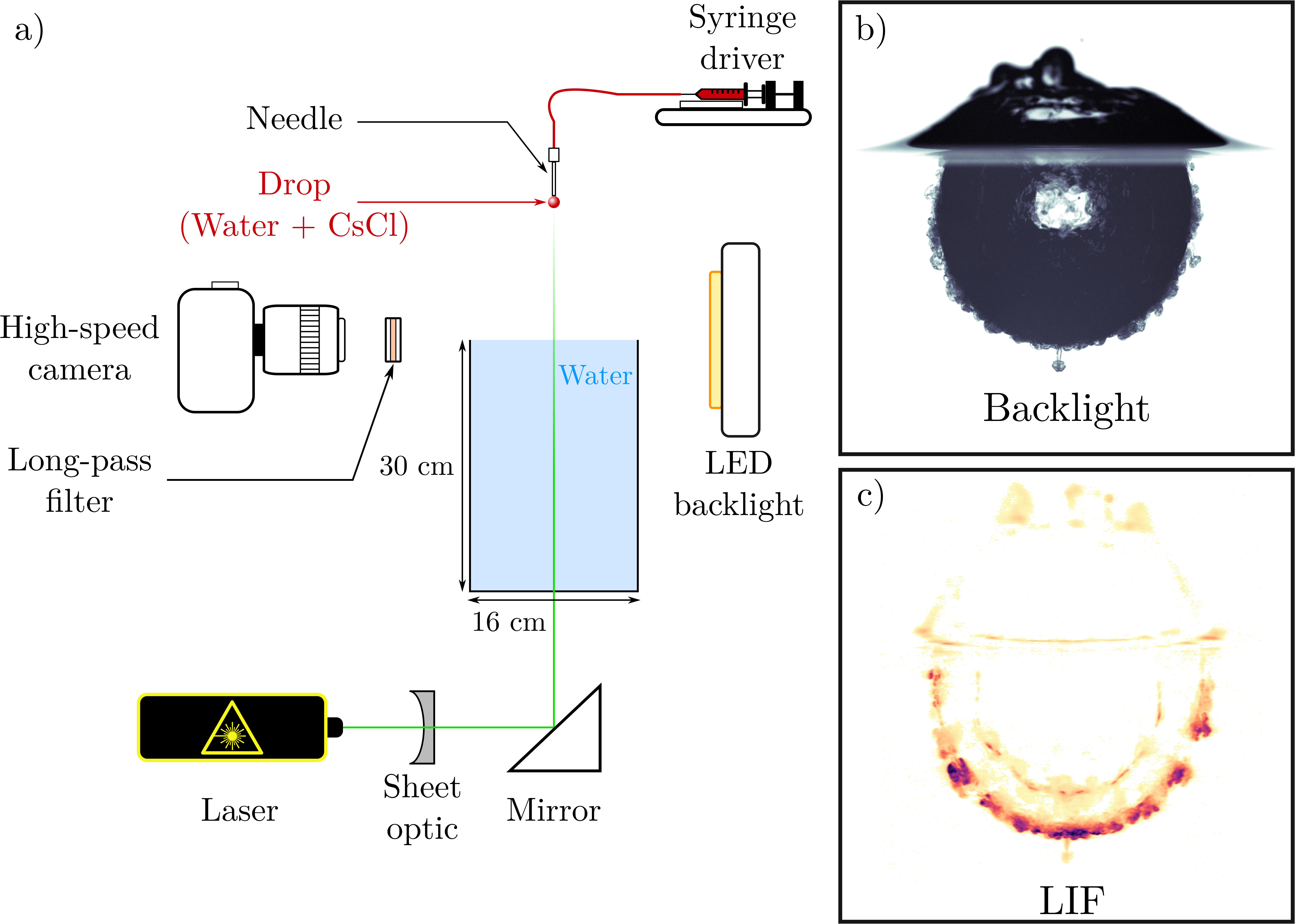
The drop is generated using a needle supplied with fluid by a syringe driver at a slow and steady pace. When the weight of the drop exceeds the stabilising surface tension effect, the drop comes off. We used a metallic needle with an inner diameter of 1.6 mm and a nylon plastic needle with an inner diameter of 4.7 mm, generating two series of drop size with typical radius in the range mm and mm, respectively. The exact drop size, which depends on the drop density, is calculated for each experiment based on a careful calibration using precise mass measurements of dozens of drops, independent density measurement, and assuming the drop is spherical. We validate this method using high-speed pictures of the drop prior to impact where we can directly measure the drop radius.
Typical impact velocities are in the range . Impact velocity is calculated for each experiment using a calibrated free fall model for the drop including a quadratic drag. We also validate this method using high-speed pictures of the drop prior to impact where we can directly measure the drop velocity.
Concerning fluids, we use an aqueous solution of caesium chloride CsCl (, ) in the drop, and water (, ) in the pool. Surface tension at the air-water interface is . The density is measured for each experiments using an Anton Paar DMA 35 Basic densitometer. Viscosities and surface tension are obtained using data from Haynes 2016.
Results are obtained with two imaging configurations, backlight and Laser-Induced Fluorescence (LIF) configurations, most suited to crater shape determination and mixing characterisation, respectively. In both configurations, the camera is positioned at the same height as the water surface. Images are recorded at 1400 Hz with a pixels resolution, and a 12 bits dynamic range, using a high-speed Phantom VEO 640L camera and a Tokina AT-X M100 PRO D Macro lens.

2.2.2 Backlight configuration
In the backlight configuration (figure 3a), we measure the evolution of the mean crater radius. The crater is illuminated from behind by a LED backlight panel and appears dark owing to refraction of light at the air-water interface. Image processing involves spatial calibration using a sight, background removal, intensity threshold, image binarization, and allows us to determine the crater boundary.
The crater boundary radius , which depends on the polar angle and time , is then fitted using a set of shifted Legendre polynomials up to degree
| (3) |
where are the fitted coefficient. The shifted Legendre polynomials are defined as an affine transformation of the standard Legendre polynomials , and are orthogonal on , i.e. on a half-space. The mean crater radius is obtained from the coefficient, i.e. .
Uncertainties are dominated by the extrinsic variability between experiments in the same configuration. Each experiment is repeated at least four times consecutively in order to estimate uncertainties on dimensionless parameters and target quantities. This allows to include uncertainties resulting from reflections and refraction at the crater boundary.
In comparison, intrinsic uncertainties related to the spatial resolution of the camera, the spatial calibration, and image processing are negligible. Spatial resolution of the camera, viz , is adequate given the size of the target, allowing this uncertainty to be neglected. Spatial calibration errors, typically around 0.2 px, are also neglected. Given the camera resolution and dynamic range, a good contrast is obtained on the crater and the impacting drop, which allows to neglect errors related to image processing.
Uncertainties on fluid properties and impact parameters are propagated to uncertainties on the dimensionless numbers (equations 1 and 2). Errors on density, viscosity and surface tension are carefully measured (density) or calculated (viscosity and surface tension) in a temperature controlled environment. Errors on the velocity and radius of the impacting drop are obtained from the variability in mass measurements and from error propagation in the velocity model, respectively.
2.2.3 Laser-Induced Fluorescence configuration
In the LIF configuration (figure 3b), we measure the thickness of the mixing layer and the number of plumes produced by the RT instability. A vertical laser sheet (532 nm) excites the fluorescent dye (Rhodamine 6G) contained in the fluid of the drop. The fluorescent dye then re-emits light between 570 nm and 660 nm. This emission signal is then recorded by the camera and isolated from the laser signal with a long-pass filter ( nm). The laser sheet is generated using a 10 W Nd:YAG continuous laser in combination with a divergent cylindrical lens and a telescope, producing a 1 mm thick sheet. The laser sheet is diverted vertically using a mirror beneath the tank. In order to isolate the mixing layer, images are processed with spatial calibration using a sight, background removal, and laser sheet corrections, removing sheet inhomogeneities. Artefacts due to reflections on the surface and on the air-water interface are then filtered and removed. In particular, the internal reflection of the mixing layer (e.g. figure 2c) is carefully removed. The dye concentration field in the mixing layer is eventually obtained, using its direct proportionality to the measured field of light intensity.
As for the backlight configuration, the position of the crater boundary , corresponding to the inner boundary of the mixing layer, is fitted using a set of shifted Legendre polynomials up to degree . A local frame of reference is then defined, where is normal to the fitted crater boundary and is tangent to it. For each polar position about the crater boundary, the local mean position of the mixing layer is calculated, using the position of the pixels in the local frame of reference and the corresponding concentration field
| (4) |
The local standard deviation about the local mean position of the mixing layer is then calculated
| (5) |
The mixing layer thickness is eventually obtained with
| (6) |
using a weighted average where is a symmetric logistic weight function whose steepness is and sigmoid’s midpoint is . The logistic function allows to give more weight to the bottom of the crater, between and , and less to the top of the crater, close to . The use of such a weight function is motivated by the polar dependency of the LIF signal quality. Close to the surface, i.e. at , signal intensity is reduced and imaging of the mixing layer undergoes significant perturbations, leading to a poor estimate of its extent. The crater is indeed illuminated from below, so that the laser sheet undergoes absorption as it goes through a dyed layer, and refraction as it goes through a layer with a variable density and index of refraction. Imaging of the mixing layer close to the surface may also be perturbed directly by the air-water interface, causing reflection of the laser sheet. All these effects can be amplified since the crater is not hemispherical. If the drop is denser than the pool, the crater is stretched downward, leading after a while to an ellipsoidal crater centred below the surface of the pool. The path of the laser sheet through the mixing layer is thus geometrically increased, and is more likely to cross the air-water interface.
The number of plumes produced by the RT instability is counted manually for each experiment at the same dimensionless time (figure 3b). It corresponds to an already developed and visible instability, where the plumes, however, did not have time to interact with each other, which is relevant since this number of plume is to be compared with theoretical results from a linear stability analysis (Chandrasekhar 1955).
As in the backlight configuration, uncertainties are dominated by the extrinsic variability between experiments in the same configuration, and each experiment is thus repeated at least four times consecutively. Intrinsic uncertainties are negligible and uncertainties on dimensionless numbers are calculated in the same way.
3 Experimental phenomenology
The phenomenology of the Rayleigh-Taylor instability is intrinsically related to the crater evolution following the impact, and particularly to its acceleration history. Using both backlight and LIF configurations, the air-water interface evolution and the mixing layer evolution are obtained, thus providing the means for a phenomenological description of the observed RT instability. The following description is based on two typical experiments, with and without density contrast, with the same crater opening dynamics, in the backlight (figure 4a,c) and the LIF configurations (figure 4b,d).
3.1 Crater geometry
The impact of the drop causes the formation of an impact crater that grows until it reaches its maximum size (figure 4a, iv). The liquid of the drop is first deformed and accumulated on the crater floor (figure 4b, i), on a timescale , akin to previous results (Bisighini et al. 2010). Then, it quickly spreads on the crater sides toward the surface (figure 4b, ii) during a timescale , eventually producing a layer with an approximately uniform thickness on the nearly hemispherical surface of the crater (figure 4b, iii-v). The impact also produces a fluid crown (Fedorchenko & Wang 2004) (figure 4a, i-iv), along with a surface wave propagating radially outward from the crater (Leng 2001) on the horizontal surface. As can be seen from the concentration field (figure 4b, i-iv), the fluid of the drop mostly accumulates on the surface of the crater, leaving a crown mainly composed of fluid from the pool. As soon as the crown decelerates, the cylindrical sheet produces liquid ligaments around the crown rim, which eventually fragment into drops (figure 4a, ii-iii) (Krechetnikov & Homsy 2009; Zhang et al. 2010; Agbaglah et al. 2013). When the crater reaches its maximum size (figure 4a, iv), crater starts to collapse (figure 4a, v). A capillary wave can develop on the crater surface (Pumphrey & Elmore 1990; Morton et al. 2000). The resulting converging flow leads to the formation of an upward jet mostly composed by the fluid of the drop, in view of the concentration field (figure 4b, vi).

3.2 Rayleigh-Taylor instability
During crater opening, after an initial impulse, the crater boundary decelerates, producing a radial deceleration more than ten times larger than vertical gravity (see section 4.2). If the density of the drop is larger than the density of the pool, it leads to an unstable equilibrium where any perturbation at the drop-pool interface is amplified radially, in the local direction of apparent gravity. This density-driven instability is interpreted as a Rayleigh-Taylor instability since the (negative) acceleration history of the interface is sustained during the whole crater opening. Although this crater deceleration decreases rapidly in magnitude, the interface acceleration is not impulsive. Thus, the instability is not an incompressible Richtmyer-Meshkov instability (Richtmyer 1960; Meshkov 1969; Jacobs & Sheeley 1996). This spherical RT instability is expected to compete with the crater geometrical expansion, that dampens its development by stretching the dense layer.
First, the instability goes through a stage where the perturbations of the interface are small in comparison with the radius of the crater and the wavelength of the instability (figure 4d, i-ii). This initial stage is expected to occur very early in the crater opening sequence, as suggested by our experiments where the perturbations reach the same size as the instability wavelength, at . This stage is not directly observed in our experiments because geometrical effects, that stretch and thin the dense layer, prevail over the RT instability. Fast vigorous crater expansion is indeed expected to dampens the RT instability. Since the two fluids involved are miscible, i.e. surface tension is zero, all wave numbers are expected to be unstable with respect to the RT instability (Chandrasekhar 1955). However, owing to larger velocity gradients at large wave numbers, viscosity is responsible for the energy dissipation of short wavelengths. The growth rate of the instability then decreases as the inverse of the wave number (Chandrasekhar 1961). Consequently, a mode of maximum instability depending on the acceleration history and impact parameters is expected to develop. This mode of maximum instability likely determines the typical number of plumes and the corresponding wavelength.
At some point, geometrical effects produced by crater expansion loose intensity and become comparable with the RT instability. This coincides with a stage where the instability is strongly influenced by three-dimensional effects, leading to the formation of plumes below the hemispherical surface of the crater (figure 4d, iii). As the RT instability grows toward a more turbulent layer, the mode of maximum instability is likely to be modified by non-linear interactions. Plumes then start interacting with each other, producing a mixing layer (figure 4d, iv). Interactions are expected to come from multi-mode perturbations interacting non-linearly with each other, and from small-scale Kelvin-Helmholtz instability produced at the side of the plumes (Cook et al. 2004).
A qualitative insight on the competition between the geometrical expansion of the crater and mixing produced by the RT instability is given with figure 5, showing the time evolution of the position of the mixing layer during crater opening. When the drop density is the same as in the pool (figure 5a), no mixing by the RT instability occurs and the drop layer only becomes thinner due to crater expansion. When the drop density is larger than the pool density (figure 5b), the mixing layer also becomes thinner due to crater expansion, but at some point, the mixing layer thickness begins to increase as the mixing produced by the RT instability starts to prevail over the geometrical expansion of the crater.

This competition also appears in figure 6, which shows the mixing layers when the crater reaches its maximum size, as a function of the Froude number and the density ratio. For density ratios smaller than unity (first column), the impacting drop is only stretched by crater expansion. Mixing related to the RT instability does not occur in this stable configuration. For density ratios about unity (second column), mixing slightly occur due to large-scale Kelvin-Helmholtz instability in the mixing layer. During crater opening, the air-water interface is not purely hemispherical and the velocity field is not purely radial (Bisighini et al. 2010). This creates a velocity shear across the interface, and sometimes produces a large-scale Kelvin-Helmholtz instability. For density ratios larger than unity (third and forth columns), mixing due to the RT instability occurs. For a given Froude number, the mixing layer thickness obtained when the crater reaches its maximum size increases with the initial density ratio. For a given density ratio, the mixing layer thickness does not change significantly with the Froude number.

4 Evolution of the crater size
Experiments in the backlight configuration provide the time evolution and the maximum of the mean crater radius, a required step in the understanding of the RT instability dynamics. We derive an energy model for the evolution of the crater radius, velocity, and acceleration and compare it with experiments. We then obtain scaling laws for the maximum crater radius and the crater opening timescale.
4.1 Energy conservation model
We use an energy conservation model (Engel 1966; Engel 1967; Leng 2001) accounting for the density difference between the impacting drop and the targeted pool. We assume a hemispherical crater associated with an incompressible and irrotational flow. Since the crater opening dynamics is mainly driven by impactor inertia and gravity forces (), viscous dissipation is not included into the model. The terms related to the formation of the crown and the surface wave during the impact, in particular their potential, kinetic, and surface energies, are not explicitly included either in the model.
On the basis of these assumptions, the sum of the crater potential energy , the crater surface energy , and the crater kinetic energy , at any instant of time is equal to the impacting drop kinetic energy just before the impact. The potential energy of the crater is
| (7) |
where is the depth. The crater surface energy corresponds to the formation of a new surface due to crater opening. This energy is related to the difference between the initially planar surface area of the pool and the hemispherical surface area of the cavity , i.e.
| (8) |
The crater kinetic energy corresponds to the kinetic energy of the pool fluid below the initial surface and is related to the flow velocity potential. A radial velocity potential of the form , solution of the Laplace equation , is able to satisfy the boundary conditions. At the crater boundary, the radial velocity is , giving and
| (9) |
The radial velocity, the tangential velocity, and the resultant velocity are respectively
| (10) |
The crater kinetic energy is then
| (11) |
The impacting drop kinetic energy is
| (12) |
Energy conservation between , , and gives
| (13) |
where and are fitted parameters. The coefficient corresponds to a correction parameter accounting for the terms not included in the model, i.e. viscous dissipation and crown energy terms. The coefficient is a correction parameter accounting for the difference between the deliberately simplified velocity potential used in the model and the true flow.
Normalising the crater radius and opening velocity by the impacting drop radius and velocity , respectively, energy conservation becomes
| (14) |
For each experiment, is calculated at . Assuming that the velocity field vanishes simultaneously in the pool (Prosperetti & Oguz 1993), the crater kinetic energy vanishes when the crater reaches its maximum size, which gives an estimate of independent of the crater opening velocity field
| (15) |
Knowing the amount of energy delivered to the pool after the impact, the time evolution of the mean crater radius is then fitted to the experiments with equation 14 using a least-square method, the kinetic energy correction parameter being a fit parameter. Knowing and , the ordinary differential equation 14 is solved using the boundary condition . This condition assumes that the crater radius is initially the same as the drop radius, at .
4.2 Time evolution
Figure 7 compares the fitted energy model with experimental data, in two reference cases, with and without density difference between the impacting drop and the pool. In both cases, the fitted mean crater radius, opening velocity, and acceleration are in close agreement with the experimental data. In the case, and . In the case, and .
At early times, the crater potential and surface energies may be neglected in comparison with the crater kinetic energy. The kinetic energy of the impactor is then balanced by the crater kinetic energy in equation 14. Using these assumptions, a power-law scaling for the crater evolution is obtained
| (16) |
where . This scaling consistently verifies the imposed boundary condition . The scaling depends on the density ratio , and on the correction parameters and . It is in agreement with experimental data at early times (figure 7, dashed lines), and similar scalings from previous works (Leng 2001; Bisighini et al. 2010).
At late times, the crater velocity becomes very small. If surface tension can be neglected, taking the time derivative of equation 14, and then making the assumption gives
| (17) |
Using and as boundary conditions, a quadratic solution is obtained
| (18) |
This scaling is in good agreement with experimental data at late times using experimental values for the boundary conditions (figure 7, dash-dotted lines). Using scaling laws for and (determined in section 4.4), the late-time quadratic evolution of the mean crater radius may be fully predicted as function of , , , and .
4.3 Energy partitioning and kinetic energy correction
Figure 8a shows the correction parameter as a function of the Froude number. Since the energy is partitioned between the impacting drop and the target, and that several energy sinks such as crown energy and viscous dissipation are neglected in the model, is expected to be smaller than unity. In our experiments, the energy partitioning coefficient is indeed , in agreement with previous works where experimental data are fitted using a partitioning coefficient in the range , depending on the Froude number (Engel 1966; Olevson 1969; Leng 2001).
Furthermore, the coefficient is found to be a decreasing function of , which scales as
| (19) |
and is relatively independent of the density ratio and the drop size. This implies that as the impactor inertia increases, the fraction of kinetic energy delivered to the target decreases. This may be explained by a change in the energy balance between the crater energy and the crown energy (Olevson 1969). As the impactor inertia increases, the relative importance of the surface energy of the crater and the crown decreases, while the potential energy of the crater and the kinetic energy of the crown increases, resulting in a global increase of the crown energy to the expense of the crater. According to Olevson 1969, the energy within the crown increases with faster than the energy within the crater, which would imply that is a decreasing function of . The drop deformation upon impact may also increase with impactor inertia, and with it the energy required for this deformation, decreasing to this extent the energy delivered to the pool.
Figure 8b shows the kinetic energy correction parameter , as a function of the Froude number. It accounts for the difference between the deliberately simplified velocity potential used in the model 9 and the true flow. Since the crater boundary is not hemispherical and the crown is necessarily generated by a tangential velocity field, the true velocity potential in not purely radial, leading to a decrease of the kinetic energy of the flow for a given crater opening velocity (Engel 1967; Bisighini et al. 2010). is very likely a function of time, but it is here assumed to be constant. In our experiments, the kinetic energy correction parameter is smaller than unity with . This means that the velocity model overestimates the crater kinetic energy in the energy balance, as expected. We do not observe any resolvable trend between , and .

4.4 Maximum crater radius and opening timescale
Assuming that the available impact kinetic energy is fully converted into crater potential energy, i.e. neglecting the crater surface energy and the kinetic energy terms, equation 14 gives a scaling for the normalised maximum crater radius
| (20) |
Figure 9a shows the normalised maximum crater size in our experiments as a function of a least-square best-fit power law scaling in the form . The exponent for is close to the theoretical prediction of equation 20, and is in agreement with previous works on liquids (Prosperetti & Oguz 1993; Leng 2001; Bisighini et al. 2010) and granular materials (Walsh et al. 2003; Takita & Sumita 2013). The prefactor is close to the value predicted by the model (equation 20). Since in our experiments, the predicted model prefactor is indeed equal to . The prefactor is also consistent with those obtained in previous works (e.g. in Leng 2001).

We now turn to estimating the crater opening time, defined as the time at which the maximum crater size is reached. Rearranging equation 14 and integrating between and gives
| (21) |
Writing with given by equation 20,
| (22) |
A first estimate of in the large limit can be obtained by neglecting the potential and surface energy terms in equation 14 (Leng 2001),
| (23) |
Figure 9b shows the normalised opening time in our experiments as a function of a least-square best-fit power law scaling in the form . The exponent for agrees with the theoretical prediction of equation 23. The exponent for is also close to the prediction of equation 23, and agrees with previous works (Leng 2001; Bisighini et al. 2010). The prefactor is close to the value predicted by equation 23, albeit somewhat larger. Since and in our experiments, the model prefactor is indeed equal to . The prefactor is also somewhat larger than the prefactors obtained in previous works (e.g. in Leng 2001).
By renormalising the crater radius and time as and , respectively, equation 14 gives
| (24) |
which depends only on the dimensionless parameter . This parameter brings in the effect of surface tension on the cratering dynamics. This is a second order effect compared to the scalings of equations 20 and 23. Figure 10a shows the time evolution of the crater radius normalised that way. The energy model (equation 14) applies only during the opening of the crater, i.e. when . Hence, experimental data collapse only when , with a residual dependency on .
At , the crater opening velocity is zero, which using equation 24 gives a corrected scaling law accounting for surface tension effects on the maximum crater radius
| (25) |
By integrating equation 24, a corrected estimate accounting for surface tension is obtained for the opening timescale
| (26) |
Substituting by in equation 26, where is the first-order development of equation 25, and developing a first-order approximation of as a function of , equation 26 gives
| (27) |
where is the beta function, , and . If surface tension is neglected, i.e. , is an exact solution of equation 26.
Figure 10b shows the maximum normalised crater radius , as a function of . It corresponds to the ratio between experimental data and the scaling law without surface tension (equation 20). As expected, the scaling overestimates the experimental maximum crater radius because it neglects surface energy, and several energy sinks related to the crown formation. This overestimate decreases with , i.e. when surface tension effects become negligible in comparison with impactor inertia and gravity forces. The difference between experimental data and the scaling law without surface tension is properly corrected by equation 25, using the surface tension term.
Figure 10c shows the normalised crater opening timescale , as a function of . It corresponds to the ratio between experimental data and the the scaling law without surface tension (equation 23). The scaling underestimates the experimental opening timescale. When surface energy and crown formation are neglected, the crater is indeed expected to open faster, i.e. on a reduced timescale. The difference between experimental data and the scaling law without surface tension is partly corrected by equation 27, giving a reasonable trend and relative errors under 20%.
5 Evolution of the Rayleigh-Taylor instability
Experiments in the LIF configuration provide the time evolution of the mixing layer. Using the energy conservation model, a model for the mixing layer thickness evolution is derived and compared with experiments. A linear stability analysis model is also used to obtain theoretical instability wavelength at early times.
5.1 Mixing layer thickness
5.1.1 Mixing model
In addition to the energy conservation model assumptions, we assume the mixing layer to be homogeneous with a constant thickness around the crater boundary.
We first consider a situation where negligible mixing occurs between the drop liquid and its surrounding. As the crater radius increases, the drop liquid spreads over an increasingly large surface area, decreasing in turn its mean thickness . Denoting by the laterally averaged velocity field associated with the opening of the crater, the time derivative of is then given by
| (28) |
Since corresponds to the radial potential flow of equation 10, this gives
| (29) |
where the right-hand side is referred to as a spreading term. This equation corresponds to the mass conservation of the layer.
We now consider a simple model of RT induced mixing (figure 11), assuming that the instability produces velocity fluctuations in the mixing layer. We thus define a scalar mixing term , which corresponds to a measure of these velocity fluctuations, and represents the mixing intensity. This mixing term corresponds to an inward flux of ambient liquid toward the mixing layer. We then assume to be the sum of the spreading and mixing terms (figure 11c), which gives
| (30) |
The velocity and length scale can be seen as the velocity and integral length-scale of a mixing-length turbulent model describing the mixing layer.
The evolution of is obtained using a buoyancy-drag model of the mixing layer (Dimonte 2000; Oron et al. 2001; Zhao et al. 2013). If we consider that the mixing layer with a density penetrates into the less dense surrounding liquid with a density , an equation of motion is
| (31) |
where and are the RT buoyancy prefactor and the drag coefficient, respectively. This equation corresponds to a balance between the fluid inertia on the left-hand side, buoyancy in the first term of the right-hand side, and inertial drag in the second term of the right-hand side. The acceleration of the crater boundary being significantly larger than , Earth’s gravity is neglected in the buoyancy term.
Using mass conservation in the homogeneous mixing layer, the dimensionless density evolution is
| (32) |
where is the initial density difference, i.e. between the impacting drop and the pool. Replacing the density evolution (equation 32) in the equation of motion eventually gives
| (33) |
Together with the crater radius evolution (equation 14), equations 30 and 33 are coupled ordinary differential equations. This initial value problem is solved numerically using , and as initial conditions. For each experiment, the experimentally measured crater radius and mixing layer thickness are used to determine the best value for the fitting parameters, which are the energy partitioning coefficient , the kinetic energy correction coefficient , the buoyancy prefactor , and the drag coefficient .
5.1.2 Time evolution
Figure 12 compares the fitted mixing layer evolution model with experimental data, in three reference cases, without density difference and with two density ratios of the impacting drop and the pool. In figure 12c, is estimated from equation 30 based on experimental measurements of and . The fitted time evolution of the mixing layer model is most of the time in agreement with experimental data. For dimensionless time typically smaller than 10, i.e. at the very beginning of the crater expansion, the model often overestimates the mean mixing layer thickness. It may be explained by model assumptions being poorly verified, such as a nearly hemispherical crater and an homogeneous mixing layer (e.g. figure 4). In the same way, in figure 12c, is overestimated for dimensionless times typically smaller than 10, for experiments with and without density difference. It means that the measured mixing layer growth rate is larger than the predicted velocity related to the geometrical evolution of the crater (equation 28). This overestimate is explained by the initial accumulation of the liquid of the drop at the crater floor. The liquid of the drop flows on the crater sides, producing a mixing layer growth rate comparatively larger than in the model with an homogeneous thickness. The overestimate indeed decreases on a timescale corresponding to the drop spread on the crater sides.
5.1.3 Buoyancy prefactor and drag coefficient
Figure 13 shows the fitted buoyancy prefactor and drag coefficient for each experiment. Our results are compared with the plane layer experiments of Dimonte 2000, who found a good agreement between their experiments and buoyancy-drag model with and .
In our experiments, the mean value of the buoyancy prefactor is , i.e. smaller than unity. This difference in the buoyancy prefactor may be interpreted as a consequence of the spherical interface, or the limited thickness of the dense layer. Given error bars, we find that may be independent of the density ratio, but may increase with the Froude number at large density ratios (), until it reaches at .
The mean value of the drag coefficient is . This value is in agreement with the value obtained for constant, variable and impulsive accelerations history (Dimonte 2000). Given error bars, we find that may decrease when the density ratio increases, the mean value of the drag coefficient at and being respectively and . As for the buoyancy prefactor, may increase with the Froude number at large density ratios (), until it reaches at .

In order to interpret and compare the values of and , two simplified acceleration history, different from the actual acceleration of the crater, are now considered: a constant acceleration and an impulsive acceleration.
In the case of a constant acceleration , the solution to the buoyancy-drag equation 31 in which geometrical effects are neglected is (Dimonte 2000, e.g.), where is a prefactor depending on several parameters such as fluid miscibility, and the fluid being penetrated, i.e. light into heavy or heavy into light. Since , and assuming that , the prefactor is
| (34) |
Figure 14a shows , calculated for each experiment, and compares the results to the homogeneous buoyancy-drag model of Dimonte 2000 calculated for , , and . The mean value is somewhat smaller than values (0.05-0.07) measured at the same density ratio between immiscible fluids, with a constant acceleration (Dimonte & Schneider 2000). Within error bars, may also increase with the density ratio. However, the homogeneous model of Dimonte 2000 overestimates the observed values of , in particular for large density ratio. For example, at the drag coefficient is approximately (figure 13b), which leads to an overestimate of by a factor 2. This may be a consequence of the variable acceleration, but also of the spherical interface, miscibility, and the limited thickness of the dense layer.
In the case of an impulsive acceleration, the buoyancy term in equation 31 is negligible since . Neglecting geometrical effects, i.e. , and assuming that , the solution is then given by , where , and and are initial values (Dimonte 2000, e.g.). The exponent is then
| (35) |
Figure 14b shows , calculated for each experiments, and compares the results to the buoyancy-drag model of Dimonte 2000. The mean value is close to values (0.2-0.3) measured at the same density ratio between immiscible fluids, with an impulsive acceleration (Dimonte & Schneider 2000). Within error bars, increases with the density ratio, consistently with the homogeneous model of Dimonte 2000 estimated at compatible values of the drag coefficient (figure 13). Since the acceleration of the crater is approximately a power-law, the acceleration is relatively close to be impulsive, explaining the good agreement between our experiments and the impulsive acceleration model.

5.1.4 Geometrical stage, mixing stage, and transition timescale
We now focus on the numerical solution of the coupled ordinary differential equations. Using figure 15, which shows the spreading term (first term on the right-hand side) and the mixing term (second term on the right-hand side) in equation 30, and the buoyancy term (first term on the right-hand side) and the drag term (second term on the right-hand side) in equation 33, as a function of time, the mixing layer evolution is decomposed into a geometrical stage and a mixing stage with a transition happening at a time .
The first stage (), referred to as the geometrical stage, corresponds to a negative growth rate of the mixing layer. Its dynamics is controlled by the geometrical evolution of the crater, with the spreading term prevailing over the RT mixing term in equation 30. Since the crater deceleration is large at early times, the buoyancy term prevails over the drag term in the buoyancy-drag equation 33. However, this does not influence the evolution of the mixing layer since the spreading term prevails.
In this stage, if the mixing term is neglected, the solution of equation 30 is
| (36) |
Using the power-law solution of (equation 16), an analytical solution is obtained for in the geometrical phase (figure 12, dashed lines). If in addition , what might be a reasonable assumption after a few dimensionless time (e.g. figure 4), equation 30 simplifies as
| (37) |
The solution corresponds to the conservation of the initial volume of the impactor, a sphere of unit dimensionless radius, which takes the form
| (38) |
Using the power-law solution of equation 16, equation 38 also gives a power-law solution for the mixing layer thickness, velocity, and acceleration
| (39) |
and consequently a power-law solution for the mixing layer growth rate
| (40) |
These solutions (figure 12, dotted lines) depend on the density ratio , and on the correction parameters and , through .
The transition time between the geometrical stage and the mixing stage can be defined as the time at which geometrical effects are of the same order of magnitude as the mixing produced by the RT instability, i.e. when the growth rate changes sign and the mixing layer thickness reaches a local minimum. The transition time between stages is determined experimentally and compared with the transition time obtained from the numerical model (figure 16a). Although uncertainties on the transition time are significant due to the extrinsic variability of experiments in the same configuration, the numerical model is rather consistent with experimental data.
An analytical estimate for the transition time is also derived. Equation 30 is simplified using approximation of equation 37 for the geometrical term, i.e. , which is supposed to be valid at the transition time. Equation 33 is also simplified assuming . These assumptions correspond to , which might be a reasonable assumption after at the transition time. Using these assumptions, equations 30 and 33 give
| (41) |
At the critical transition time , geometrical effects are of the same order of magnitude as mixing effects, which means that (equation 30). Using in addition the power-laws solutions of (equation 16) and (equation 39) in the geometrical stage, an estimate of is obtained from equation 41
| (42) |
where is a least-squares best-fit prefactor obtained from experimental data (figure 16b). As expected in figure 12, the transition time decreases with the density contrast between the fluid of the impacting drop and the pool. The larger the density contrast, the quicker mixing effects become comparable to geometrical effects.

The second stage (), referred to as the mixing stage, corresponds to a positive growth rate of the mixing layer. Its dynamics is controlled by a balance between residual geometrical effects and mixing produced by the RT instability. The spreading term and the mixing term are then similar in magnitude. Since the drag term prevails over the buoyancy term because the crater deceleration vanishes, the mixing term is consequently controlled by the drag term. At late times, when the crater is close to reach its maximum, the spreading term vanishes and the mixing layer dynamics is only controlled by the mixing term.
In this stage, equation 30 may be simplified using approximation of equation 37 for the geometrical term, which is supposed to be valid in the mixing stage. Equation 33 is simplified neglecting the buoyancy term and assuming . These assumptions respectively correspond to the vanishing crater deceleration and during the mixing stage. Using these assumptions, equations 30 and 33 become
| (43) |
Assuming a power-law solution for (equation 16), and using and as initial conditions, a solution to equation 43 is
| (44) |
where (figure 12, dash-dotted lines). The value required to fit experimental data is smaller than the value obtained by fitting experimental data with the full numerical model (equations 16, 30 and 33). If the latter was used, the analytical solution would underestimate the layer thickness in the mixing stage since the value of depends strongly on the assumption made to obtain this solution, i.e. approximated geometrical term, neglected buoyancy term, , and power-law for .
5.1.5 Maximum mixing layer thickness
Figure 17 shows the mixing layer thickness , growth rate , and the estimated mixing term as a function of time, for all experiments, grouped by density ratio. The maximum layer thickness increases significantly with the initial density ratio (figure 17a). In the mixing stage (typically ), an increased initial density difference promotes mixing by the RT instability, but leads only to a slight increase of the mixing layer growth rate (figure 17b) and the estimated mixing term (figure 17c). The increase of the maximum layer thickness with the initial density ratio is in fact controlled by the time window available for the mixing layer to actually grow. On one hand, the transition time , i.e. the time at which geometrical effects become comparable to RT mixing, corresponds to the lower limit of the available time window. Since decreases when the initial density ratio increases (equation 42), expanding in this way the time window, it is consistent with the increasing effect of the density ratio on the maximum layer thickness. On the other hand, the maximum opening timescale , i.e. the time at which the crater radius reaches a maximum, corresponds to the upper limit of the available time window. being an increasing function of the density ratio (equation 23), it is also consistent with the increasing effect of the density ratio on the maximum thickness. Since also increases with the Froude number, the time window available for the mixing layer to develop, and consequently the maximum thickness, may also increase with the Froude number.

The experimental maximum mixing layer thickness is first compared with the maximum thickness obtained from the model (figure 18a), leading to a good agreement. Since the maximum layer thickness is expected to depend on both the initial density ratio and the Froude number through power-laws, experimental data are then fitted using a power-law scaling (figure 18b). A good agreement is obtained using
| (45) |
where , and . This scaling is consistent with the qualitative observations of figure 6, i.e. a maximum mixing layer thickness increasing with the initial density ratio and the Froude number. Given the scalings for and , it also agrees with an increased time window available for the mixing layer to develop.

5.2 Early-time wavelength
Experimental instability wavelengths at early times are converted into an equivalent spherical harmonic degree, and compared to a scaling law and to an approximate linear stability analysis model (Chandrasekhar 1955). From the number of plumes , counted on the hemispherical section of the density interface at , a typical instability wavelength is derived. The corresponding degree of maximum instability is then obtained using the Jeans relation (Jeans 1923)
| (46) |
Concerning the scaling law, the instability wavelength is assumed to depend on the balance between an effective mixing layer acceleration and the viscosity of the ambient fluid , which respectively produce and damp the instability. The scaling for the wavelength is then , which after nondimensionalization gives
| (47) |
Assuming that and respectively scale as and (see equations 20 and 23), and using the Jeans relation (equation 46), the scaling for the wavelength gives a scaling for the degree of maximum instability
| (48) |
where is a least-squares best-fit prefactor obtained from experimental data (figure 19a).
Harmonic degrees of maximum instability are shown in figure 19a, for all experiments, as a function of their derived scaling . Experimental data are mostly proportional to the scaling, except for Reynolds number smaller than 4000. In this case, the crater differs from the hemispherical shape and from the purely radial acceleration assumed in the scaling.

Experimental results are also compared to a linear stability analysis model (Chandrasekhar 1955). An incompressible fluid sphere having a density and a viscosity is radially accelerated into an ambient fluid having a density and a viscosity . The mean radius of the sphere is assumed to be constant with time. Perturbations at the interface are expanded in spherical harmonics of degree . Using a variational principle, an approximate dispersion relation for the growth rate of the instability is obtained
| (49) |
with
| (50) |
This dispersion relation, corresponding to a dimensionless version of equation 90 in Chandrasekhar 1955, is in agreement with exact results derived by Chandrasekhar 1955.
The growth rate of the instability is obtained by solving simultaneously the dispersion relation (equation 49) and the mean crater radius evolution (equation 14). The time evolution of the theoretical growth rate as a function of the spherical harmonic degree is thus obtained for all experiments (e.g. figure 19b). The time evolution derives from the time dependent terms of equation 49, i.e. and . Since the model of Chandrasekhar 1955 is a static model, i.e. the average position of the density interface is constant with time, results should be considered carefully. The dynamic problem, i.e. with a moving density interface, is much more challenging (Prosperetti 1977, e.g.) and will not be addressed here. At a given time, the instability growth rate reaches a maximum owing to viscosity effects, giving the theoretical degree of maximum instability (figure 19b). For small degrees, the instability growth rate scales as , as expected from inviscid planar geometry cases (Rayleigh 1899; Taylor 1950). For large degrees, viscosity effects start to develop due to the larger velocity gradients involved. Viscosity dissipates short wavelength energy, leading to a decay of the instability growth rate, as in viscous planar geometry without surface tension (Chandrasekhar 1961).
In order to compare the model with experimental data, the theoretical degree of maximum instability is calculated at , i.e. the time at which the experimental degree of maximum instability is measured. Figure 19c shows a close agreement between experimental data and the model, except for Reynolds number smaller than 4000, as previously explained.
6 Geophysical implications
After the impact, the metal core of the colliding body migrates toward the planetary core due to the density contrast with the surrounding silicates (Rubie et al. 2015). Part of the migration occurs in a fully molten magma ocean where the metal is expected to descend as a turbulent thermal and equilibrate with silicates (Deguen et al. 2011; Deguen et al. 2014). The metal phase then undergoes a vigorous stirring (Lherm & Deguen 2018), leading to its fragmentation (Landeau et al. 2014; Wacheul et al. 2014; Wacheul & Le Bars 2018) into centimetric drops (Stevenson 1990; Karato & Murthy 1997; Rubie et al. 2003; Ichikawa et al. 2010). However, these models assume that the metal cores are released as a compact volume in the magma ocean, which is not true after a planetary impact (Kendall & Melosh 2016; Landeau et al. 2020). Their initial conditions may be improved by considering the impact stage.
In order to estimate the mixing produced by the spherical RT instability during the opening stage of planetary impacts, a relevant quantity is the mass of ambient silicates that mixes with the impacting core during crater opening (Deguen et al. 2014). If an impactor with a radius , a volume fraction of metal , a metal core density , and a silicate mantle density , impacts a planetary target, the dimensionless mass of equilibrated silicates is , where is the mass of the metal core and is the mass of entrained silicates. After nondimensionalization, the mass of silicates mixed with metal gives
| (51) |
Using scaling laws for (equation 20), (equation 45), and implicitly (equation 19), a scaling law for the mixing mass is obtained
| (52) |
where , and . In this scaling, the density ratio is defined with , where is the mean density ratio of the impactor, because it derives from the crater size and the maximum mixing layer thickness scalings (equations 20 and 45, respectively), which indeed use the mean density of the impactor. This scaling law is validated on experimental data in figure 20a, using since the drop is a one-phase fluid.

In the context of planetary impacts, the Froude number is given by
| (53) |
where is the escape velocity, and is the radius of the target planet. The impact velocity of colliding bodies during accretion is typically one to three times the escape velocity (Agnor et al. 1999; Agnor & Asphaug 2004), which means that the Froude number depends mainly on the target to impactor radius ratio. is about 1 for giant impacts, comparable in size to the target, but increases by several order of magnitude for small colliding bodies.
Using equations 52 and 53, the estimated mass of silicates mixed with the impacting core during crater opening is calculated as a function of the target to impactor radius ratio (figure 20b). We use and to match the internal structure of a realistic differentiated impactor (Canup 2004). Since the Froude number increases with the target to impactor radius ratio, it means that a smaller colliding body will produce more mixing, relative to their size, than giant impactors. For example, impactors with a 10 km and 100 km radius (figure 20b, triangle and circle, respectively) will then mix with 36.1 and 8.1 times its own mass, respectively.
Concerning the Moon-forming impact, the canonical impact scenario with a Mars-sized impactor (Canup 2004) is expected to mix with 0.4 times its own mass during this crater opening stage (figure 20b, square). However, the fast-spinning impact scenario associated with a faster () and smaller () colliding body (Cuk & Stewart 2012) is expected to mix with 2.3 times its own mass (figure 20b, diamond). Recent experiments estimate the mass of equilibrated silicates during the impact, considering both the crater formation, its collapse into an upward jet, and the collapse of the jet (Landeau et al. 2020). In the same conditions, the 100 km radius impactor, the canonical Moon-forming impactor and the fast-spinning Earth impactor respectively mix with 168, 1.5 and 12 times the impactor mass. It corresponds to 4 to 20 times the mass mixed by the spherical RT instability, which is in agreement with an impact-induced mixing mostly dominated by the collapse of the jet (Landeau et al. 2020). These giant impacts scenario involve small target to impactor radius, corresponding to an extrapolated range of Froude number, i.e. (figure 20b, dashed lines), which is outside of the experimental Froude number range. The mass of equilibrated silicates extrapolated for large impactor thus has to be considered carefully.
7 Conclusion
A phenomenological description of impact cratering experiments has shown that crater deceleration after impact is responsible for a density-driven perturbation at the drop-pool interface, interpreted as a spherical Rayleigh-Taylor instability. An energy conservation model for the crater radius evolution has been derived (equation 14) and compared with backlight experiments, resulting in scaling laws for the maximum crater radius (equation 20) and the opening timescale (equation 23). In combination with this energy model, a mixing layer evolution model involving two stages has been derived (equations 30 and 33). The mixing layer dynamics is first controlled by the geometrical evolution of the crater, then by the balance between residual geometrical effects and mixing produced by the Rayleigh-Taylor instability. Scaling laws for the transition timescale between stages (equation 42) and the maximum mixing layer thickness (equation 45) are obtained. The instability wavelength is also investigated using a an approximate linear stability analysis model (equations 49-50), and a scaling law is obtained (equation 48). These results have geophysical implications concerning the differentiation of terrestrial planets, in particular by estimating the mass of silicates that equilibrate with the core of the impactors during the impact of planetesimals on a magma ocean.
When experimental scaling laws are extrapolated to planetary conditions, we assume that physical processes observed in the experiments are self-similar at the planetary scale.
In order to validate these scaling laws, new experiments involving larger impactors are required to obtain Froude numbers relevant to giant impacts, and investigate the possible effect of the Reynolds number on the mixing layer.
Furthermore, several physical aspects neglected in our experiments have to be investigated experimentally or numerically, in order to examine their effect on cratering and mixing dynamics.
For giant impacts, geometrical effects related to the sphericity of both the impactor and the target, and to impact angle, may influence metal/silicate equilibration.
Immiscibility between metal and silicates may also change the mixing dynamics, in particular with the fragmentation of the metal phase. In this context, the viscosity and diffusivity contrasts may influence thermal and chemical transfers between phases.
Finally, since planetary impact velocities are larger than the sound velocity in silicates, the role of shock waves and compressibility effects, i.e. the Mach number, on cratering and mixing scaling laws has to be investigated.
This project has received funding from the European Research Council (ERC) under the European Unions Horizon 2020 research and innovation programme (grant agreement 716429). We thank M. Moulin for the help with the design and construction of the experimental apparatus and J. Vatteville for the help with the imaging equipment.
References
- Agbaglah et al. (2013) Agbaglah, Gilou, Josserand, Christophe & Zaleski, Stéphane 2013 Longitudinal instability of a liquid rim. Physics of Fluids 25 (2), 022103, publisher: American Institute of Physics.
- Agnor & Asphaug (2004) Agnor, Craig & Asphaug, Erik 2004 Accretion Efficiency during Planetary Collisions. The Astrophysical Journal 613 (2), L157–L160, publisher: IOP Publishing.
- Agnor et al. (1999) Agnor, Craig B., Canup, Robin M. & Levison, Harold F. 1999 On the Character and Consequences of Large Impacts in the Late Stage of Terrestrial Planet Formation. Icarus 142 (1), 219–237.
- Arnett et al. (1989) Arnett, W. David, Bahcall, John N., Kirshner, Robert P. & Woosley, Stanford E. 1989 Supernova 1987A. Annual Review of Astronomy and Astrophysics 27 (1), 629–700, publisher: Annual Reviews.
- Badro et al. (2018) Badro, James, Aubert, Julien, Hirose, Kei, Nomura, Ryuichi, Blanchard, Ingrid, Borensztajn, Stephan & Siebert, Julien 2018 Magnesium Partitioning Between Earth’s Mantle and Core and its Potential to Drive an Early Exsolution Geodynamo. Geophysical Research Letters 45 (24), 13,240–13,248.
- Badro et al. (2015) Badro, James, Brodholt, John P., Piet, Hélène, Siebert, Julien & Ryerson, Frederick J. 2015 Core formation and core composition from coupled geochemical and geophysical constraints. Proceedings of the National Academy of Sciences 112 (40), 12310–12314.
- Balakrishnan & Menon (2011) Balakrishnan, Kaushik & Menon, Suresh 2011 Characterization of the Mixing Layer Resulting from the Detonation of Heterogeneous Explosive Charges. Flow, Turbulence and Combustion 87 (4), 639–671.
- Bell (1951) Bell, George I 1951 Taylor instability on cylinders and spheres in the small amplitude approximation. Los Alamos Scientific Laboratory, Los Alamos, NM, Technical Report No. LA-1321 .
- Berberović et al. (2009) Berberović, Edin, van Hinsberg, Nils P., Jakirlić, Suad, Roisman, Ilia V. & Tropea, Cameron 2009 Drop impact onto a liquid layer of finite thickness: Dynamics of the cavity evolution. Physical Review E 79 (3), 036306, publisher: American Physical Society.
- Bisighini et al. (2010) Bisighini, Alfio, Cossali, Gianpietro E., Tropea, Cameron & Roisman, Ilia V. 2010 Crater evolution after the impact of a drop onto a semi-infinite liquid target. Physical Review E 82 (3), 036319.
- Canup (2004) Canup, Robin M. 2004 Simulations of a late lunar-forming impact. Icarus 168 (2), 433–456.
- Canup (2012) Canup, Robin M. 2012 Forming a Moon with an Earth-like Composition via a Giant Impact. Science 338 (6110), 1052–1055.
- Chambers (2010) Chambers, J. 2010 Terrestrial Planet Formation. In Exoplanets (ed. S. Seager), pp. 297–317. Tucson, Arizona, USA: University of Arizona Press.
- Chandrasekhar (1955) Chandrasekhar, S. 1955 The character of the equilibrium of an incompressible fluid sphere of variable density and viscosity subject to radial acceleration. The Quarterly Journal of Mechanics and Applied Mathematics 8 (1), 1–21.
- Chandrasekhar (1961) Chandrasekhar, S. 1961 Hydrodynamic and Hydromagnetic Stability. Oxford: Clarendon.
- Cook et al. (2004) Cook, Andrew W., Cabot, William & Miller, Paul L. 2004 The mixing transition in Rayleigh–Taylor instability. Journal of Fluid Mechanics 511, 333–362, publisher: Cambridge University Press.
- Corgne et al. (2007) Corgne, Alexandre, Keshav, Shantanu, Fei, Yingwei & McDonough, William F. 2007 How much potassium is in the Earth’s core? New insights from partitioning experiments. Earth and Planetary Science Letters 256 (3), 567–576.
- Cuk & Stewart (2012) Cuk, Matija & Stewart, Sarah T. 2012 Making the Moon from a Fast-Spinning Earth: A Giant Impact Followed by Resonant Despinning. Science 338 (6110), 1047–1052.
- Dalziel et al. (1999) Dalziel, S. B., Linden, P. F. & Youngs, D. L. 1999 Self-similarity and internal structure of turbulence induced by Rayleigh–Taylor instability. Journal of Fluid Mechanics 399, 1–48, publisher: Cambridge University Press.
- Deguen et al. (2014) Deguen, Renaud, Landeau, Maylis & Olson, Peter 2014 Turbulent metal–silicate mixing, fragmentation, and equilibration in magma oceans. Earth and Planetary Science Letters 391, 274–287.
- Deguen et al. (2011) Deguen, Renaud, Olson, Peter & Cardin, Philippe 2011 Experiments on turbulent metal-silicate mixing in a magma ocean. Earth and Planetary Science Letters 310 (3), 303–313.
- Dimonte (1999) Dimonte, Guy 1999 Nonlinear evolution of the Rayleigh–Taylor and Richtmyer–Meshkov instabilities. Physics of Plasmas 6 (5), 2009–2015, publisher: American Institute of Physics.
- Dimonte (2000) Dimonte, Guy 2000 Spanwise homogeneous buoyancy-drag model for Rayleigh–Taylor mixing and experimental evaluation. Physics of Plasmas 7 (6), 2255–2269, publisher: American Institute of Physics.
- Dimonte & Schneider (2000) Dimonte, Guy & Schneider, Marilyn 2000 Density ratio dependence of Rayleigh–Taylor mixing for sustained and impulsive acceleration histories. Physics of Fluids 12 (2), 304–321, publisher: American Institute of Physics.
- Emmons et al. (1960) Emmons, H. W., Chang, C. T. & Watson, B. C. 1960 Taylor instability of finite surface waves. Journal of Fluid Mechanics 7 (2), 177–193, publisher: Cambridge University Press.
- Engel (1966) Engel, Olive G. 1966 Crater Depth in Fluid Impacts. Journal of Applied Physics 37 (4), 1798–1808.
- Engel (1967) Engel, Olive G. 1967 Initial Pressure, Initial Flow Velocity, and the Time Dependence of Crater Depth in Fluid Impacts. Journal of Applied Physics 38 (10), 3935–3940.
- Fedorchenko & Wang (2004) Fedorchenko, Alexander I. & Wang, An-Bang 2004 On some common features of drop impact on liquid surfaces. Physics of Fluids 16 (5), 1349–1365.
- Fischer et al. (2015) Fischer, Rebecca A., Nakajima, Yoichi, Campbell, Andrew J., Frost, Daniel J., Harries, Dennis, Langenhorst, Falko, Miyajima, Nobuyoshi, Pollok, Kilian & Rubie, David C. 2015 High pressure metal–silicate partitioning of Ni, Co, V, Cr, Si, and O. Geochimica et Cosmochimica Acta 167, 177–194.
- Gielen et al. (2017) Gielen, Marise V., Sleutel, Pascal, Benschop, Jos, Riepen, Michel, Voronina, Victoria, Visser, Claas Willem, Lohse, Detlef, Snoeijer, Jacco H., Versluis, Michel & Gelderblom, Hanneke 2017 Oblique drop impact onto a deep liquid pool. Physical Review Fluids 2 (8), 083602.
- Haynes (2016) Haynes, William M. 2016 CRC Handbook of Chemistry and Physics. CRC Press.
- Ichikawa et al. (2010) Ichikawa, H., Labrosse, S. & Kurita, K. 2010 Direct numerical simulation of an iron rain in the magma ocean. Journal of Geophysical Research 115 (B01404), 1–12.
- Jacobs & Sheeley (1996) Jacobs, J. W. & Sheeley, J. M. 1996 Experimental study of incompressible Richtmyer–Meshkov instability. Physics of Fluids 8 (2), 405–415, publisher: American Institute of Physics.
- Jain et al. (2019) Jain, Utkarsh, Jalaal, Maziyar, Lohse, Detlef & Meer, Devaraj van der 2019 Deep pool water-impacts of viscous oil droplets. Soft Matter 15 (23), 4629–4638.
- Jalaal et al. (2019) Jalaal, Maziyar, Kemper, Dave & Lohse, Detlef 2019 Viscoplastic water entry. Journal of Fluid Mechanics 864, 596–613.
- Jeans (1923) Jeans, James Hopwood 1923 The propagation of earthquake waves. Proceedings of the Royal Society of London. Series A, Containing Papers of a Mathematical and Physical Character 102 (718), 554–574, publisher: Royal Society.
- Karato & Murthy (1997) Karato, Shun-ichiro & Murthy, VR. 1997 Core formation and chemical equilibrium in the Earth—I. Physical considerations. Physics of the Earth and Planetary Interiors 100 (1), 61–79.
- Kendall & Melosh (2016) Kendall, Jordan D. & Melosh, H. J. 2016 Differentiated planetesimal impacts into a terrestrial magma ocean: Fate of the iron core. Earth and Planetary Science Letters 448, 24–33.
- Kleine et al. (2002) Kleine, T., Münker, C., Mezger, K. & Palme, H. 2002 Rapid accretion and early core formation on asteroids and the terrestrial planets from Hf–W chronometry. Nature 418 (6901), 952.
- Krechetnikov & Homsy (2009) Krechetnikov, Rouslan & Homsy, George M. 2009 Crown-forming instability phenomena in the drop splash problem. Journal of Colloid and Interface Science 331 (2), 555–559.
- Labrosse et al. (2007) Labrosse, S., Hernlund, J. W. & Coltice, N. 2007 A crystallizing dense magma ocean at the base of the Earth’s mantle. Nature 450 (7171), 866.
- Landeau et al. (2014) Landeau, M., Deguen, R. & Olson, P. 2014 Experiments on the fragmentation of a buoyant liquid volume in another liquid. Journal of Fluid Mechanics 749, 478–518.
- Landeau et al. (2020) Landeau, M., Deguen, R., Phillips, D., Neufeld, J. A., Lherm, V. & Dalziel, S. B. 2020 Metal-Silicate Mixing by Large Earth-forming impacts. Submitted to Earth and Planetary Science Letters .
- Leng (2001) Leng, Liow Jong 2001 Splash formation by spherical drops. Journal of Fluid Mechanics 427, 73–105.
- Lherm & Deguen (2018) Lherm, V. & Deguen, R. 2018 Small-Scale Metal/Silicate Equilibration During Core Formation: The Influence of Stretching Enhanced Diffusion on Mixing. Journal of Geophysical Research: Solid Earth 123 (12), 10,496–10,516.
- Lhuissier et al. (2013) Lhuissier, H., Sun, C., Prosperetti, A. & Lohse, D. 2013 Drop Fragmentation at Impact onto a Bath of an Immiscible Liquid. Physical Review Letters 110 (26), 264503.
- Li & Agee (1996) Li, Jie & Agee, Carl B. 1996 Geochemistry of mantle–core differentiation at high pressure. Nature 381 (6584), 686.
- Lin et al. (2002) Lin, Hao, Storey, Brian D. & Szeri, Andrew J. 2002 Rayleigh–Taylor instability of violently collapsing bubbles. Physics of Fluids 14 (8), 2925–2928, publisher: American Institute of Physics.
- Linden et al. (1994) Linden, P. F., Redondo, J. M. & Youngs, D. L. 1994 Molecular mixing in Rayleigh–Taylor instability. Journal of Fluid Mechanics 265, 97–124, publisher: Cambridge University Press.
- Lindl (1998) Lindl, John 1998 Inertial Confinement Fusion: The Quest for Ignition and Energy Gain Using Indirect Drive. American Inst. of Physics.
- Lombardini et al. (2014) Lombardini, M., Pullin, D. I. & Meiron, D. I. 2014 Turbulent mixing driven by spherical implosions. Part 1. Flow description and mixing-layer growth. Journal of Fluid Mechanics 748, 85–112, publisher: Cambridge University Press.
- Macklin & Metaxas (1976) Macklin, W. C. & Metaxas, G. J. 1976 Splashing of drops on liquid layers. Journal of Applied Physics 47 (9), 3963–3970, publisher: American Institute of Physics.
- Melosh (1989) Melosh, H. J. 1989 Impact cratering: A geologic process. New York: Oxford University Press.
- Meshkov (1969) Meshkov, E. E. 1969 Instability of the interface of two gases accelerated by a shock wave. Fluid Dynamics 4 (5), 101–104.
- Mikaelian (1990) Mikaelian, Karnig O. 1990 Rayleigh-Taylor and Richtmyer-Meshkov instabilities and mixing in stratified spherical shells. Physical Review A 42 (6), 3400–3420.
- Mikaelian (2016) Mikaelian, Karnig O. 2016 Viscous Rayleigh-Taylor instability in spherical geometry. Physical Review E 93 (2), 023104.
- Monteux et al. (2011) Monteux, J., Jellinek, A. M. & Johnson, C. L. 2011 Why might planets and moons have early dynamos? Earth and Planetary Science Letters 310 (3), 349–359.
- Morton et al. (2000) Morton, David, Rudman, Murray & Jong-Leng, Liow 2000 An investigation of the flow regimes resulting from splashing drops. Physics of Fluids 12 (4), 747–763.
- Nakajima et al. (2020) Nakajima, Miki, Golabek, Gregor J., Wünnemann, Kai, Rubie, David C., Burger, Christoph, Melosh, Henry J., Jacobson, Seth A., Manske, Lukas & Hull, Scott D. 2020 Scaling laws for the geometry of an impact-induced magma ocean. arXiv:2004.04269 [astro-ph] ArXiv: 2004.04269.
- Okawa et al. (2006) Okawa, Tomio, Shiraishi, Takuya & Mori, Toshiaki 2006 Production of secondary drops during the single water drop impact onto a plane water surface. Experiments in Fluids 41 (6), 965.
- Olevson (1969) Olevson, K. L. R. 1969 Energy balances for transient water craters. US Geol. Surv. Prof. Pap D (650), 189–194.
- Oron et al. (2001) Oron, D., Arazi, L., Kartoon, D., Rikanati, A., Alon, U. & Shvarts, D. 2001 Dimensionality dependence of the Rayleigh–Taylor and Richtmyer–Meshkov instability late-time scaling laws. Physics of Plasmas 8 (6), 2883–2889, publisher: American Institute of Physics.
- Plesset (1954) Plesset, M. S. 1954 On the Stability of Fluid Flows with Spherical Symmetry. Journal of Applied Physics 25 (1), 96–98.
- Prosperetti (1977) Prosperetti, Andrea 1977 Viscous effects on perturbed spherical flows. Quarterly of Applied Mathematics 34 (4), 339–352.
- Prosperetti & Oguz (1993) Prosperetti, A & Oguz, H N 1993 The Impact of Drops on Liquid Surfaces and the Underwater Noise of Rain. Annual Review of Fluid Mechanics 25 (1), 577–602.
- Pumphrey & Elmore (1990) Pumphrey, Hugh C. & Elmore, Paul A. 1990 The entrainment of bubbles by drop impacts. Journal of Fluid Mechanics 220, 539–567.
- Ray et al. (2015) Ray, Bahni, Biswas, Gautam & Sharma, Ashutosh 2015 Regimes during liquid drop impact on a liquid pool. Journal of Fluid Mechanics 768, 492–523.
- Rayleigh (1899) Rayleigh, John William Strutt 1899 Scientific papers (Vol. 2: 1881-1887). Cambridge University Press.
- Rein (1993) Rein, Martin 1993 Phenomena of liquid drop impact on solid and liquid surfaces. Fluid Dynamics Research 12 (2), 61–93.
- Richtmyer (1960) Richtmyer, Robert D. 1960 Taylor instability in shock acceleration of compressible fluids. Communications on Pure and Applied Mathematics 13 (2), 297–319, _eprint: https://onlinelibrary.wiley.com/doi/pdf/10.1002/cpa.3160130207.
- Righter (2011) Righter, K. 2011 Prediction of metal–silicate partition coefficients for siderophile elements: An update and assessment of PT conditions for metal–silicate equilibrium during accretion of the Earth. Earth and Planetary Science Letters 304 (1), 158–167.
- Rubie et al. (2011) Rubie, David C., Frost, Daniel J., Mann, Ute, Asahara, Yuki, Nimmo, Francis, Tsuno, Kyusei, Kegler, Philip, Holzheid, Astrid & Palme, Herbert 2011 Heterogeneous accretion, composition and core–mantle differentiation of the Earth. Earth and Planetary Science Letters 301 (1), 31–42.
- Rubie et al. (2003) Rubie, D. C., Melosh, H. J., Reid, J. E., Liebske, C. & Righter, K. 2003 Mechanisms of metal–silicate equilibration in the terrestrial magma ocean. Earth and Planetary Science Letters 205 (3), 239–255.
- Rubie et al. (2015) Rubie, D. C., Nimmo, F. & Melosh, H. J. 2015 Formation of the Earth’s Core. In Treatise on Geophysics (Second Edition) (ed. Gerald Schubert), pp. 43–79. Oxford: Elsevier.
- Rudge et al. (2010) Rudge, John F., Kleine, Thorsten & Bourdon, Bernard 2010 Broad bounds on Earth’s accretion and core formation constrained by geochemical models. Nature Geoscience 3 (6), 439.
- Scherstén et al. (2006) Scherstén, Anders, Elliott, Tim, Hawkesworth, Chris, Russell, Sara & Masarik, Jozef 2006 Hf–W evidence for rapid differentiation of iron meteorite parent bodies. Earth and Planetary Science Letters 241 (3), 530–542.
- Schmidt (2006) Schmidt, Wolfram 2006 From tea kettles to exploding stars. Nature Physics 2 (8), 505–506.
- Siebert et al. (2012) Siebert, Julien, Badro, James, Antonangeli, Daniele & Ryerson, Frederick J. 2012 Metal–silicate partitioning of Ni and Co in a deep magma ocean. Earth and Planetary Science Letters 321-322, 189–197.
- Siebert et al. (2011) Siebert, Julien, Corgne, Alexandre & Ryerson, Frederick J. 2011 Systematics of metal–silicate partitioning for many siderophile elements applied to Earth’s core formation. Geochimica et Cosmochimica Acta 75 (6), 1451–1489.
- Solomatov (2015) Solomatov, V. 2015 Magma Oceans and Primordial Mantle Differentiation. In Treatise on Geophysics (Second Edition) (ed. Gerald Schubert), pp. 81–104. Oxford: Elsevier.
- Stevenson (1990) Stevenson, D. J. 1990 Fluid dynamics of core formation. In Origin of the earth (ed. Horton E. Newsom & John H. Jones), pp. 231–249. New York: Oxford University Press.
- Stixrude et al. (2009) Stixrude, Lars, de Koker, Nico, Sun, Ni, Mookherjee, Mainak & Karki, Bijaya B. 2009 Thermodynamics of silicate liquids in the deep Earth. Earth and Planetary Science Letters 278 (3), 226–232.
- Sun et al. (2018) Sun, Yicheng, Zhou, Huiqun, Yin, Kun, Zhao, Mengqi, Xu, Shijin & Lu, Xiancai 2018 Transport Properties of Fe2SiO4 Melt at High Pressure From Classical Molecular Dynamics: Implications for the Lifetime of the Magma Ocean. Journal of Geophysical Research: Solid Earth 123 (5), 3667–3679.
- Takita & Sumita (2013) Takita, Haruna & Sumita, Ikuro 2013 Low-velocity impact cratering experiments in a wet sand target. Physical Review E 88 (2), 022203.
- Taniguchi (1988) Taniguchi, H. 1988 Surface tension of melts in the system CaMgSi2O6-CaAl2Si2O8 and its structural significance. Contributions to Mineralogy and Petrology 100 (4), 484–489.
- Taylor (1950) Taylor, Geoffrey Ingram 1950 The instability of liquid surfaces when accelerated in a direction perpendicular to their planes. I. Proceedings of the Royal Society of London. Series A. Mathematical and Physical Sciences 201 (1065), 192–196, publisher: Royal Society.
- Thomas & Kares (2012) Thomas, V. A. & Kares, R. J. 2012 Drive Asymmetry and the Origin of Turbulence in an ICF Implosion. Physical Review Letters 109 (7), 075004, publisher: American Physical Society.
- Tonks & Melosh (1993) Tonks, W. Brian & Melosh, H. Jay 1993 Magma ocean formation due to giant impacts. Journal of Geophysical Research: Planets 98 (E3), 5319–5333.
- Tryggvason (1988) Tryggvason, Grétar 1988 Numerical simulations of the Rayleigh-Taylor instability. Journal of Computational Physics 75 (2), 253–282.
- Wacheul & Le Bars (2018) Wacheul, Jean-Baptiste & Le Bars, Michael 2018 Experiments on fragmentation and thermo-chemical exchanges during planetary core formation. Physics of the Earth and Planetary Interiors 276, 134–144.
- Wacheul et al. (2014) Wacheul, Jean-Baptiste, Le Bars, Michael, Monteux, Julien & Aurnou, Jonathan M. 2014 Laboratory experiments on the breakup of liquid metal diapirs. Earth and Planetary Science Letters 403, 236–245.
- Walsh et al. (2003) Walsh, Amanda M., Holloway, Kristi E., Habdas, Piotr & de Bruyn, John R. 2003 Morphology and Scaling of Impact Craters in Granular Media. Physical Review Letters 91 (10), 104301, publisher: American Physical Society.
- Wille et al. (2002) Wille, G., Millot, F. & Rifflet, J. C. 2002 Thermophysical Properties of Containerless Liquid Iron up to 2500 K. International Journal of Thermophysics 23 (5), 1197–1206.
- Williams & Nimmo (2004) Williams, Jean-Pierre & Nimmo, Francis 2004 Thermal evolution of the Martian core: Implications for an early dynamo. Geology 32 (2), 97–100.
- Wood et al. (2006) Wood, Bernard J., Walter, Michael J. & Wade, Jonathan 2006 Accretion of the Earth and segregation of its core. Nature 441 (7095), 825.
- Worthington (1895) Worthington, A. M. 1895 The splash of a drop. London, UK: London, S.P.C.K.
- Youngs & Williams (2008) Youngs, David L. & Williams, Robin J. R. 2008 Turbulent mixing in spherical implosions. International Journal for Numerical Methods in Fluids 56 (8), 1597–1603, _eprint: https://onlinelibrary.wiley.com/doi/pdf/10.1002/fld.1594.
- Zhang et al. (2010) Zhang, Li V., Brunet, Philippe, Eggers, Jens & Deegan, Robert D. 2010 Wavelength selection in the crown splash. Physics of Fluids 22 (12), 122105, publisher: American Institute of Physics.
- Zhao et al. (2013) Zhao, B., Law, A. W. K., Lai, A. C. H. & Adams, E. E. 2013 On the internal vorticity and density structures of miscible thermals. Journal of Fluid Mechanics 722.