On the controversial turbulent Schmidt number value in particle-laden boundary layer flowsPreprint: APS/123-QED
Abstract
One of the most enigmatic science question concerning inertial particle transport by a turbulent boundary layer flow is the value of the turbulent Schmidt number defined as the ratio of turbulent eddy viscosity to particle concentration diffusivity. Using direct acoustic measurement of turbulent particle flux profile, and two-phase flow turbulence-resolving numerical simulation, it is demonstrated that turbulent dispersion of particles is reduced rather than enhanced as predicted by many existing literature models. The explanation lies in the misleading assumption of settling velocity in quiescent water to estimate the turbulent particle diffusivity, while direct measurements and simulations of turbulent particle flux support the occurrence of settling retardation. The analysis presented herein suggests that the value of the turbulent Schmidt number is always larger than unity with values between 3 and 4 based on the directly measured turbulent particle flux. The observed settling reduction can not be explained by the well-known hindrance effects related to particle concentration. This effect seems to be related to turbulence-particle interactions and correlates more with the Stokes number. At last, the new parameters, namely the turbulent Schmidt number higher than unity, modified von Kármán constant, and settling retardation, are successfully tested for the modeling of particle concentration profile using the well-known Rouse formulation. This result suggests that new parametrizations are possible to reduce the degree of empiricism to predict suspended particle transport by a boundary layer flow.
I Introduction
The transport of solid particles by a turbulent fluid flow is a key process in geophysical and industrial two-phase flows such as material and food processing, pneumatic transport, fluidized beds, slurry flows or sediment transport. In all these situations, interactions between particles and fluid turbulence are key physical processes that contribute to the dynamics of the system. Among the consequences induced by the presence of particles, the modification of fluid turbulence and the turbulent dispersion of particles are crucial mechanisms that are not fully understood Balachandar and Eaton 2010. The complexity arises when particles are inertial, i.e. when the particle response time is larger than a representative turbulent eddy time-scale , leading to Stokes number greater than unity. Inertial particles act as a local filter for the turbulent kinetic energy spectrum due to their not fully-correlated movements with turbulent eddies of similar or smaller size than the particle itself. This problem has been studied in many different flow configurations including Homogeneous Isotropic Turbulence, jets and turbulent wall-bounded flows. However, further complexity arises under gravitational acceleration.
In sediment transport, under intense flows corresponding to high fluid bed shear stress relative to the buoyant weight of the particles, the so-called Shields number , strong erosions from the underlying sediment bed are observed and a significant amount of particles are transported in suspension by fluid turbulent eddies Garcia 2008. The coupling between the sediment flux and the underlying bed topography controls the large-scale morphological evolution of rivers, estuaries and coastal nearshore zones Aagaard and Hughes 2010. In most of these situations, the transported particles are made of inorganic non-cohesive sand grains with Stokes number values well above unity, i.e. inertial particles. Sediment transport is a truly multi-scale process coupling fine scale turbulence-particle interactions (O() - O(ms)) with the morphological evolution of natural systems at large scales (O() - O(yrs)). Therefore, elucidation of the governing interaction processes associated with the transport of inertial particles by a turbulent boundary layer flow is a major scientific issue.
The quantity of particular interest is the stream-wise particle flux defined as the integral over the flow depth of the product between the local particle velocity and particle concentration. Consequently, it is necessary to understand the key processes that controls the velocity and concentration profiles. On the one hand, the presence of particles may significantly modify turbulence (Vanoni 1975; Kiger and Pan 2002; Revil-Baudard et al. 2015; Cheng et al. 2018, e.g.). This is often characterized by a modification of the von Kármán constant in the classical logarithmic law-of-the-wall. On the other hand, the turbulent diffusivity of particle concentration may significantly differ from the fluid eddy-viscosity Lyn 2008. These two quantities are the key ingredients to predict the particle flux. Under fully-developped turbulent flow conditions and by assuming a local balance between the gravity-driven settling flux and the upward Reynolds particle flux , the particle phase mass conservation equation reduces to:
| (1) |
In this equation, is the particle settling velocity and is the wall-normal Reynolds particle flux. In the later, stands for the velocity fluctuations and for the concentration fluctuations defined with respect to their respective mean values where represents a temporal averaging operator. Rouse 1938 proposed to model the Reynolds particle flux using a Fickian gradient diffusion model:
| (2) |
where , the particle concentration turbulent diffusivity, is linked to the eddy-viscosity through the turbulent Schmidt number defined as . Using a Prandtl’s mixing length model with a free surface correction for the eddy-viscosity , where is the von Kármán constant, is the wall-normal distance and is the water depth above the particle bed and by further assuming that particle settling velocity can be approximated by its value in quiescent water , Rouse 1938 derived an analytical solution for the mean particle concentration profile as:
| (3) |
where is a reference concentration taken at an elevation above the particle bed and located within the suspension layer, i.e. where , and is the Rouse number corresponding to the slope of the particle concentration profile. In this definition, represents the bed friction velocity. Using measured concentration profile and the estimated bed friction velocity and particle settling velocity, the Schmidt number can be readily estimated using the Rouse profile.
Discrepancies between a measured concentration profile and the Rouse profile have been attributed to a modification of the particle diffusivity compared with the eddy viscosity, leading to values of the turbulent Schmidt number different from unity. Because this classical method estimates the Schmidt number by best fitting the measured concentration profile with the Rouse profile and leaving as the only free parameter, the resulting is a depth-averaged value noted as in the following. Figure 1a summarizes several experimental values reported in the literature for plotted as a function of Lyn 2008. The first observation that can be made is the large scatter of the data with values lower and higher than unity. Values lower (higher) than unity can be interpreted as an enhanced (reduced) dispersion of particles compared to fluid momentum. Van Rijn 1984 suggested that turbulent dispersion of inertial particles is enhanced due to centrifugal force which tends to throw particles out of small-scale turbulent vortexes and proposed an empirical model written as:
| (4) |
While this model (solid line in Figure 1a) is widely used, it does not match the laboratory data of Lyn 1988.
The turbulent Schmidt number can also be obtained locally provided that the concentration profile is measured with enough accuracy to resolve the sharp wall-normal gradients near the flow bed. Figure 1b shows a summary of existing data for locally estimated Schmidt number as a function of the normalized depth . Again shows large scatter with values ranging from as low as 0.2 to as large as 2.5. In the experiments reported by Lyn 1988 and Barton and Lin 1955, only the mean concentration profile was measured and so is obtained by using both the mass balance and the gradient diffusion model (Eqs. 1-2) and therefore under the assumption that . In Cellino and Graf 1999, using the novel acoustic particle flux profiler of Shen and Lemmin 1999, the authors measured directly the turbulent particle flux and hence only Eq. 2 is used to calculate directly. The mean concentration profile used to estimate was obtained from an iso-kinetic flow suction system with a much lower vertical resolution than the direct measurement of the Reynolds particle flux Cellino 1998. This introduces a source of uncertainty in their results especially in the near-bed region where the concentration gradient is very high. Despite this source of measurement uncertainty, it is interesting to point out that almost all their data (circles in 1b) suggest .
The potential reasons for the discrepancies in the Schmidt number values reported in the literature are (i) the assumption of using particle settling velocity in quiescent water and (ii) the assumption of the von Kármán constant value being identical to the clear water value (). Concerning the first assumption, several publications have reported that the settling velocity of individual particles could be modified in turbulent flows Murray 1970; Good et al. 2014; Cuthbertson and Ervine 2007; Kawanisi and Shiozaki 2008; Zhou and Cheng 2009; Akutina et al. 2020; Mora et al. 2021. However, no consensus has been reached on the effect of turbulence on the settling velocity of individual particles as some studies have found settling velocity enhancement while others observed settling retardation (Nielsen 1992; Kawanisi and Shiozaki 2008; Dey et al. 2019, e.g.). Regarding the second assumption, in particle-laden flows, von Kármán constant reduction has been reported (Vanoni 1941; Revil-Baudard et al. 2015; Revil-Baudard et al. 2016, e.g.). Two physical mechanisms have been proposed to explain this reduction, density stratification Vilaret and Davies 1995 and/or turbulent drag work Hsu et al. 2003; Cheng et al. 2018. The fact that the ratio appears in the Rouse number definition could explain some of the observed discrepancies. In order to address this question, it is mandatory to measure concurrently and with sufficient accuracy the velocity and the concentration profiles to allow for a direct estimate of the von Kármán constant and of the turbulent Schmidt number. This ability represents a major measurement challenge under such energetic particle-laden flow conditions.
To the best of our knowledge, the first measurements reported in the literature showing turbulent fluxes, mean concentration and velocity profiles are those of Shen and Lemmin 1999 using the Acoustic Particle Flux Profiler. Over the past ten years, we have intensively developed and improved this technology as the Acoustic Concentration and Velocity Profiler (ACVP) offering a unique wide-band multi-frequency capability for simultaneous vertical profiles of velocity and particle concentration at turbulence resolving scales ( mm ; Hz) Hurther and Thorne 2011; Hurther et al. 2011; Thorne and Hurther 2014; Naqshband et al. 2017; Fromant et al. 2018; Fromant et al. 2019. We successfully applied this technology to study intense sediment transport processes in the so-called sheet-flow regime in Revil-Baudard et al. 2015. This unique data-set allows for the first time to investigate the relationship between Reynolds particle flux, Reynolds stresses, and velocity and particle concentration gradients in order to shed new light on the turbulent Schmidt number value.
Over the last two decades, significant progress has been made on the numerical modeling of sediment transport by using two-phase flow approaches (Chauchat and Guillou 2008; Jha and Bombardelli 2010; Revil-Baudard and Chauchat 2013; Lee et al. 2016; Cheng et al. 2017; Chauchat 2018, e.g.). Recently, we have performed the first turbulence-resolving two-fluid simulation Cheng et al. 2018 that has been validated against experimental data from Revil-Baudard et al. 2015. In this approach, the most energetic turbulent flow scales are directly resolved as well as the particle dynamics allowing the majority of turbulent particle fluxes to be resolved.
In this contribution, using the recent high-resolution experimental data-set of Revil-Baudard et al. 2015 and turbulence-resolving two-phase flow simulations of Cheng et al. 2018, we are able to provide a physical explanation for the contradictory findings in the literature.

II Material and method
II.1 Sediment transport experiments
In Revil-Baudard et al. 2015 sediment transport experiments have been carried out in the LEGI/ENSE3 tilting flume. The mobile bed experiment is denoted as and corresponds to a Shields number of where and are fluid and particle densities, is gravity acceleration and is the particle diameter ; and a suspension number of (see table 1). For this experiment the slope has been set to . The experimental condition has been realized times for in order to verify the reproducibility of the experiment and to perform ensemble averaging. The experimental parameters are presented in table 1.
The ACVP technology was used to measure the vertical profiles, from the non-moving particle bed up to the free-surface, of the two velocity components and of the particle volumetric concentration with vertical spatial resolution of mm at 78 Hz (see Thorne and Hurther 2014 for details on acoustic measurement method and Revil-Baudard et al. 2015; Revil-Baudard et al. 2016 for details on the specific ACVP settings applied in the datasets used herein).
| Name | Reference | |||||||||
|---|---|---|---|---|---|---|---|---|---|---|
| () | () | () | () | |||||||
| Revil-Baudard et al. 2015 | 186 | 17.4 | 178.8 | |||||||
| Shen and Lemmin 1999 | 1.3 | 1.9 | 2.3 | |||||||
| Shen and Lemmin 1999 | 1.3 | 2.2 | 2.7 |
A specific experimental protocol has been applied to obtain steady and uniform flow conditions in the absence of a particle recirculating facility. First, the time period for which the flow is uniform is identified based on the vertical linearity of the mean turbulent shear-stress profile. Then the local and instantaneous velocity, concentration and particle flux measurements are temporally averaged over and over the realizations of the same experiment to guarantee statistically converged velocities, concentration and particle flux profiles.
| (5) |
The operator refers to the superficial averaging, and is a given measured quantity. The averaging time window is s.
In order to discuss and confirm the validity of the results obtained for RB15 experiments, the experimental dataset of Shen and Lemmin 1999 will be used for comparison and referred to as runs SL99_1 and SL99_2 in the following. To the best of our knowledge, it is the only existing experimental dataset providing the required direct measurements of time-resolved vertical profiles of two components velocity, particle concentration and fluxes in similar type of particle-laden flows. The SL99 experiments were carried out in similar open-channel flow conditions regarding the hydrodynamic regimes (fully turbulent, fully hydraulically rough, uniform, steady and subcritical flows). Run SL99_2 is somewhat more energetic than SL99_1 in terms of hydraulic power but similar regarding the hydrodynamic and sediment transport regimes. The particles (sand grains of well-sorted unimodal size distribution) used in the two SL99 experiments explain the important differences seen in Table I for the suspension number, particle Reynolds and Stokes numbers values. These values reveal a fully suspension dominated particle-laden flow (with negligible bedload transport). This is due to the less inertial sand grains having much smaller size but higher density compared with the PMMA particles used in RB15. Finally, another important point is that for all considered particle-laden flows, transport capacity was fully established. This implies that concentration effects are at their maximal possible level for all considered fluid-particle interaction processes.
II.2 Two-fluid turbulence-resolving simulations
In the two-fluid turbulence-resolving or Large Eddy Simulations (LES) model, the large-scale turbulent structures are directly computed from filtered Navier-Stokes equations while the small-scale motions, occurring at spatial scales smaller than the filter size, are accounted for using sub-grid closures. In this numerical approach, both the fluid phase and the particle phase are modeled as a continuum. A Favre filtering approach is used for the scale separation, and the filtered continuity equations read as,
| (6) |
| (7) |
where is the filtered particle volumetric concentration, are the filtered fluid and particle velocities, and represents streamwise (), spanwise () and vertical () components, respectively.
The filtered momentum equations for fluid phase and particle phase are written as:
| (8) | |||||
| (9) |
where is the gravitational acceleration and is the fluid pressure. and are the fluid (molecular) viscous stress and subgrid stress associated with the unresolved turbulent motions. In analogy to the fluid phase, the unresolved particle motions due to turbulence are taken into account by the subgrid stress, . These subgrid stresses are modeled using a dynamic Smagorinsky subgrid closure (Germano et al. 1991; Lilly 1992). The particle pressure and particle stress due to intergranular interactions are modeled by the kinetic theory of granular flows (Ding and Gidaspow 1990) and phenomenological closure of contact stresses (Srivastava and Sundaresan 2003). represents the filtered drag force between fluid phase and particle phase, which is only composed of the resolved part in the present work:
| (10) |
where is the resolved relative velocity between fluid phase and particle phase. Contrary to Cheng et al. 2018 the sub-grid drag model is ignored in the present work.
The details of the numerical configuration can be found in Chauchat et al. 2017; Cheng et al. 2018 and the major parameters are summarized in table 2). Spatial averaging over the two statistically homogeneous and directions and time averaging are applied to the simulation results over a duration of about 60 eddy turn over time s to obtain ensemble-averaged flow statistics.
| run name | N cells | |||||
|---|---|---|---|---|---|---|
| (in millions) | (s) | (mm) | (mm) | (mm) | (mm) | |
| 29.2 | 1.65 | 1.65 | 0.4 | 2.2 |
III Results and discussion
In the following, our unique high-resolution experimental dataset, denoted as RB15, and two-fluid turbulence-resolving simulation results, denoted as two-fluid LES, are analyzed to infer whether or (see table 1).
The averaged profiles of velocity, concentration, Reynolds shear stress and particle flux corresponding to this configuration are presented in figure 2. Measured Reynolds stress (symbols in Figure 2c) peaks near the top of the sheet flow layer (particle volumetric concentration about 0.08) and shows the expected upward-decaying linear profile valid for steady, uniform channel flows. Within the sheet flow layer, Reynolds stress decays sharply towards the bed. Measured particle flux in the wall-normal direction also peaks at the same vertical location (Figure 2d). The results obtained using two-fluid LES are compared with measured data from Revil-Baudard et al. 2015 in figure 2. In terms of velocity and concentration profiles (Figure 2a and b) the numerical results are in good agreement with the measured data although particle concentration in the dilute suspension region is underestimated. The numerical results reproduce measured Reynolds stress very well. However, the vertical turbulent particle flux is over-predicted (resp. under-predicted) in the near bed region (resp. in the outer layer). This probably explains the discrepancies on the concentration profile observed in the two-fluid LES results. These discrepancies are still an open question. It is important to recall here that the maximum of the wall-normal turbulent flux is located in the near-bed region where the particle concentration is high, i.e. . At such volumetric concentrations a strong interplay between turbulence-particle interactions and particle-particle interactions, the so-called four-way coupling, is taking place. It is highly possible that some of the closures of the two-fluid model requires modifications to better reproduce the measurements. This issue deserves further investigations but more experimental data are needed to guide the development of the two-fluid model.


In order to avoid any uncertainties associated with a modification of the von Kármán constant, the eddy viscosity is calculated directly as:
| (11) |
To better illustrate the change in the von Kármán constant value, figure 3a presents the turbulent mixing length ). The dashed black line in the figure represents the best-fit of the analytical model where the slope of the line is the von Kármán constant. As pointed out in Revil-Baudard et al. 2015, the von Kármán constant value obtained in the experiment is , a significantly lower value than 0.41 expected for clear water flow conditions. The two-fluid LES reproduces this reduction very well. The modification of the von Kármán ”constant” value has significant fundamental consequences for boundary layer modeling in particle-laden flows. Furthermore, as already mentioned, the von Kármán ”constant” appears at the denominator of the Rouse number and severely impacts suspended particle transport modeling.
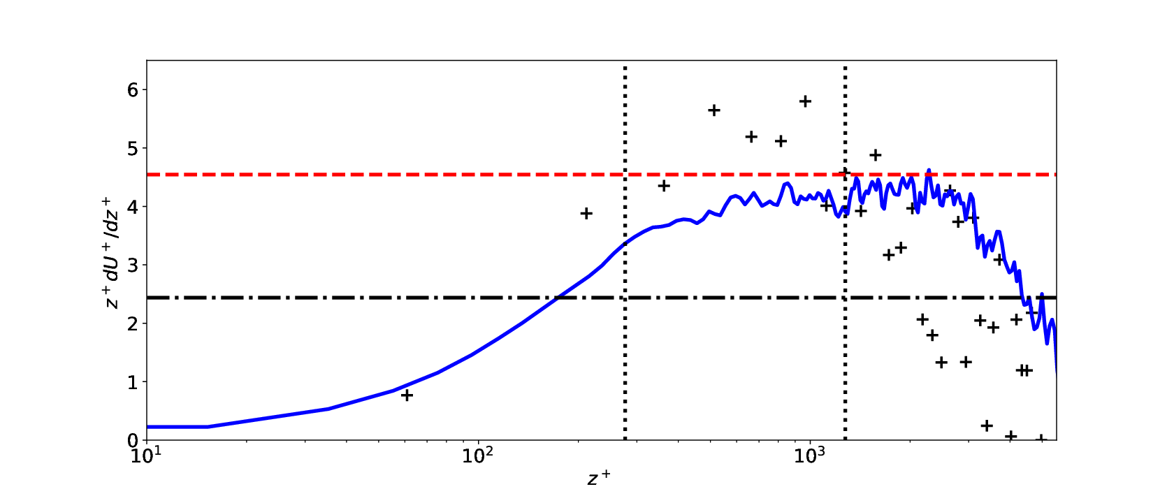
In order to confirm the existence of the logarithmic layer in this particle-laden flow configuration, the classical diagnostic for single phase flows is presented. It consists in plotting the product as a function of (Smits et al. 2011, e.g.). A first difficulty to overcome in particle-laden flows over erodible beds is the definition of the origin for . In this work, we suggest to use , the virtual origin of the mixing length:
Figure 4 shows the as a function of in semi-logarithmic scale. Both RB15 data and the two-fluid LES exhibit a plateau confirming the existence of the log-layer. The range of over which the log layer exists does not correspond exactly with the classical values for single phase flows: with (vertical dotted lines in figure 4). This difference may be attributed either to the definition of the origin of or to turbulence modifications induced by the presence of particles. Nevertheless, the existence of a plateau confirm that the flow velocity follow a logarithmic profile. The range retained to estimate the von Kármán constant is corresponding to with our definition of .
The classical method to estimate the turbulent Schmidt number is indirect and uses Eq. 1 by assuming a local balance between the gradient-diffusion model (Eq. (2)) and the gravity-driven settling flux with the particle settling velocity estimated by its value in quiescent water:
| (12) |
This quantity will be denoted as and is shown in figure 3b. For , is more or less constant with a value below unity for RB15 data and for two-fluid LES results. The model proposed by Van Rijn 1984 (see Eq. 4) gives a value of which is very close to the experimental value.
The direct method is based on the measured or simulated eddy viscosity and Reynolds particle flux (Eq. 2). Using these quantities, the turbulent Schmidt number can be calculated without using Eq. 1 as:
| (13) |
This quantity will be denoted as and is shown in figure 3c. The profiles are almost constant for , and the measured is about 4 in RB15 while the two-fluid LES confirms a value of well above unity, even-though slightly smaller. As mentioned above, measurement of the Reynolds particle flux remains a particularly challenging task which, to the best of the authors knowledge, has only been provided to date in Shen and Lemmin 1999 and Revil-Baudard et al. 2015 for similar type of particle-laden open-channel flows. Our analysis demonstrated that the estimation of Schmidt number is highly dependent on the methodology used.
In a multi-phase flow approach, it is well-known that inertial particles cannot respond instantaneously to the wide range of fluid velocity fluctuations that exists in a highly turbulent flow. The particle dynamics may be significantly different from that of the fluid parcels Balachandar and Eaton 2010. Particle inertia is estimated using the particle Stokes number where is the Kolmogorov time-scale associated with the smallest turbulent eddies. Inertial particles correspond to which is the case for the configurations investigated herein (see table 1). This supports the observation that turbulent dispersion of particles should be less efficient than turbulent mixing of fluid momentum i.e. . Therefore, the indirect estimate of turbulent Schmidt number lower than unity is hypothesized to be due to reduction of settling velocity in the settling flux. In order to prove this point, a dimensionless settling velocity is deduced from the mass balance equation, as:
| (14) |
This quantity is plotted in figure 3d which shows an almost constant value in the dilute suspended-load layer () for both RB15 and two-fluid LES results. The measured quantity shows that the settling velocity is about ten times smaller than the one in quiescent water i.e. . Recently Akutina et al. 2020, using the same PMMA particles as the one used in RB15 experiments, have measured a strong settling retardation for individual particles in a turbulence water column under quasi-homogeneous and isotropic turbulent flow conditions. In these experiments, the turbulence was generated by facing pairs of vertical grids oscillating horizontally. The measured settling velocity of individual particles has been observed to drastically decrease with increasing turbulence intensity . Using five different particle types covering a wide range of size, density and settling velocity in quiescent water, the authors have shown that all the data points for the dimensionless settling velocity as a function of the dimensionless turbulent intensity collapse on a master curve given by:
| (15) |
for . In the present open-channel flow experiment, the vertical turbulent intensity can be estimated as cm/s and Eq. (15) gives a value of . This value is very close to the one shown in figure 3d.
The two-fluid LES also predicts settling retardation () even though the reduction is less strong than in the experiments. Despite the discrepancy in magnitude, both numerical and measured values strongly support the hypothesis that settling retardation is responsible for the indirectly measured Schmidt number value smaller than unity.
To further support our hypothesis, the measured data reported by Shen and Lemmin 1999 are further examined using the same methodology as described above. The hydrodynamic conditions of these two runs (red and green symbols in Figures 5 and 6) are very similar to RB15 flow conditions (see figure 5 and table 1), the major difference concerns the particles properties that are denser and smaller, leading to smaller inertia (see section II.A), with a suspended particle concentration two orders of magnitude smaller.


Figure 6a shows the mixing length profiles with a von Kármán constant value very close to 0.41. This suggests that for lower suspended particle concentration, no reduction of the von Kármán constant is observed. In figure 6b, the turbulent Schmidt number shows a similar trend as for RB15 in the near wall region where the value is lower than unity but the scatter in Shen and Lemmin 1999 increases away from the wall where exceeds unity. The vertical profiles of are shown in figure 6c. Almost all data reveal values well above unity supporting lower turbulent particle concentration diffusivity compared to eddy-viscosity. Finally, the vertical profile of the dimensionless settling velocity is shown in figure 6d. Both runs exhibit values smaller than unity confirming the hypothesis of settling retardation but with a weaker magnitude. Furthermore, the profiles increase linearly with distance from the bed whereas the RB15 data exhibit a fairly constant value.
Both experimental datasets Revil-Baudard et al. 2015; Shen and Lemmin 1999 and the two-fluid LES Cheng et al. 2018 support the conclusion that the actual turbulent Schmidt number is higher than unity and that settling retardation plays an important role in sediment transport. In the following, we will use existing data to strengthen the analysis on settling retardation in turbulent flow. In figure 7a the dimensionless settling velocity is plotted as a function of the local volumetric concentration in semi-log scale to test the hypothesis of hindrance effects. The dashed line in the figure represents the classical Richardson and Zaki 1954 empirical formula . Clearly, the observed reduction of settling velocity can not be explained by hindrance effect. Indeed settling reduction occurs for volumetric concentration as low as for Shen and Lemmin 1999 data and there is almost no variation with in RB15 data. In figure 7b the dimensionless settling velocity is plotted as a function of as suggested by Akutina et al. 2020. As already pointed out, the scaling proposed by Akutina et al. 2020 is compatible with RB15 data, however experiments by Shen and Lemmin 1999 corresponds to which are out of Akutina et al. 2020 experimental range. It would be interesting to test this range of in the settling column to conclude on the observed trends in Shen and Lemmin 1999 data but this is beyond the scope of the present contribution. In figure 7c, the dimensionless settling velocity is plotted as a function of where the Kolmogorov time-scale has been evaluated as with . The choice of is justified by the anisotropy of the turbulence in the near-bed region and the focus on the wall-normal particle-flux that is driven by wall-normal velocity fluctuations. Using this local estimation, the Stokes number shows that it is lower than unity for Shen and Lemmin 1999 and higher than unity for Revil-Baudard et al. 2015 data (the data in this panel are only plotted in the region ). Therefore, the observed differences between the two datasets may be attributed to the differences in particles inertia but this would deserve further investigations based on experimental data over a wider range of flow conditions and particle properties.
In order to evaluate the consequences of settling retardation and turbulent Schmidt number higher than unity on volumetric concentration profile prediction, Eq. (1) is integrated numerically from to :
| (16) |
Using , and the result of Eq. (16) is denoted as Rouse Orig in figure 8 while using and measured (using fit from figure 6 for SL99_1 and 2) the result of Eq. (16) is denoted as Rouse New in figure 8. For RB15, the dash dotted line is obtained by using and but with as deduced from the fit in figure 3. The original Rouse formulation provides poor predictions of concentration profiles for all cases. The correction provided by fails to predict the slope of the concentration profiles for SL99_1 and SL99_2. For RB15 data with high sediment concentration, the modification of the von Kármán constant has a significant impact on the prediction illustrating the importance of accounting for turbulence modifications, i.e. modification of , in the prediction of suspended particle concentration. For all cases, using a turbulent Schmidt number and a dimensionless settling velocity provides the best prediction. Nevertheless, the rather crude resolution in SL99_1 and 2 data and the limited range of parameters investigated herein is not sufficient to give definitive conclusion on the parametrization for the Rouse profile.
| Name | Reference | |||||
|---|---|---|---|---|---|---|
| Revil-Baudard et al. 2015 | 0.046 | |||||
| Shen and Lemmin 1999 | 0.052 | |||||
| Shen and Lemmin 1999 | 0.053 |


IV Conclusion
In summary, the results presented herein reveals that the uncertainties on the value of the turbulent Schmidt number can be explained by a shortcoming in the methodology, and the real value of the turbulent Schmidt number estimated from directly measured Reynolds particle flux is larger than unity, and that the settling velocity is significantly reduced even at very low particle concentration. In the experiments with ”large” plastic particles, the dimensionless settling velocity is almost constant in the near bed region, however, for fine sand particles, the settling velocity is linearly increasing with the distance from the bed. A comparison with existing models reveals that the observed settling reduction can not be explained by hindrance effects, while turbulence-particle interactions are most probably responsible for this behavior. Another important result presented here concerns the modification of turbulence in the boundary layer and its consequences on suspended particle profile. In Revil-Baudard et al. 2015 measurements and two-fluid LES the von Kármán constant is reduced by a factor two. The consequences of this turbulence modification on particle concentration profile are huge and definitely needs to be accounted for in the Rouse profile parametrization.
In conclusion, innovative highly-resolved measurement technique and numerical simulations allow us to obtain new insight that changes the paradigm of suspended particle transport in a boundary layer flow. We have demonstrated that (i) turbulent dispersion of inertial particles is significantly smaller than that of fluid parcels and does not depend much on particle size and density and (ii) settling velocity of inertial particles is reduced and this reduction depends on particle size and density. This suggests that the particle properties are sensitive parameters in this problem but the details of the underlying physical mechanisms are still to be elucidated. Beyond the importance for sediment transport predictions, these findings are relevant to a wide range of two-phase flows such as avalanches, turbidity currents, pneumatic transport and particle deposition in material processing.
Data availability
The data and post-processing script used to write the manuscript are available on zenodo at the following address https://zenodo.org/record/5765565#.Ya_L7VPjJHt (see reference Chauchat et al. 2021).
Acknowledgements.
J. Chauchat is financially supported by the french ANR project SHEET-FLOW (ANR-18-CE01-0003). D. Hurther is supported by the french DGA-funded ANR Astrid Maturation project MESURE (ANR-16-ASMA-0005). Z. Cheng and T.-J. Hsu are supported by U.S. Strategic Environmental Research and Development Program (SERDP, MR20-1478) and National Science Foundation (OCE-1635151). The computations presented in this paper were performed using the GENCI infrastructure under Allocations A0060107567 and A0080107567 and the GRICAD infrastructure. The authors would like to thank N. Mordant and P. Frey for their constructive comments on the manuscript.References
- Balachandar and Eaton (2010) S Balachandar and John K Eaton, “Turbulent dispersed multiphase flow,” Annual Review of Fluid Mechanics 42, 111–133 (2010).
- Garcia (2008) Marcelo Garcia, Sedimentation Engineering (American Society of Civil Engineers, 2008) https://ascelibrary.org/doi/pdf/10.1061/9780784408148 .
- Aagaard and Hughes (2010) Troels Aagaard and Michael G. Hughes, “Breaker turbulence and sediment suspension in the surf zone,” Marine Geology 271, 250 – 259 (2010).
- Vanoni (1975) V. A. Vanoni, Sedimentation engineering (Am. Soc. Coastal Eng., 1975).
- Kiger and Pan (2002) K. T. Kiger and C. Pan, “Suspension and turbulence modification effects of solid particulates on a horizontal turbulent channel flow,” J. Turbulence 19, 1 – 21 (2002).
- Revil-Baudard et al. (2015) Thibaud Revil-Baudard, Julien Chauchat, David Hurther, and Pierre-Alain Barraud, “Investigation of sheet-flow processes based on novel acoustic high-resolution velocity and concentration measurements,” Journal of Fluid Mechanics 767, 1–30 (2015).
- Cheng et al. (2018) Zhen Cheng, Tian-Jian Hsu, and Julien Chauchat, “An eulerian two-phase model for steady sheet flow using large-eddy simulation methodology,” Advances in Water Resources 111, 205 – 223 (2018).
- Lyn (2008) D. A. Lyn, “Turbulence models for sediment transport engineering,” in Sedimentation Engineering (ASCE, 2008) Chap. Chapter 16.
- Rouse (1938) H. Rouse, “Experiments on the mechanics of sediment suspension,” in ICAM (1938) pp. 550–554.
- Van Rijn (1984) L. C. Van Rijn, “Sediment transport, part ii: Suspended load transport,” J. Hydraul. Eng. 110, 1613–1641 (1984).
- Lyn (1988) D. A. Lyn, “A similarity approach to turbulent sediment-laden flows in open channels,” Journal of Fluid Mechanics 193, 1–26 (1988).
- Barton and Lin (1955) J. R. Barton and P.-N. Lin, A study of the sediment transport in alluvial streams, Tech. Rep. (Civil Engineering Dept., Colorado A & M College, Fort , Colorado, 1955).
- Cellino and Graf (1999) M. Cellino and W. H. Graf, “Sediment-laden flow in open-channels under noncapacity and capacity conditions,” Journal of Hydraulic Engineering 125, 455–462 (1999).
- Shen and Lemmin (1999) C. Shen and U. Lemmin, “Application of an acoustic particle flux profiler in particleladen open-channel flow,” Journal of Hydraulic Research 37, 407–419 (1999), https://doi.org/10.1080/00221686.1999.9628256 .
- Cellino (1998) M. Cellino, Experimental study of suspension flow in open channels, Ph.D. thesis, Swiss Federal Institute of Techn. Lausanne (1998).
- Murray (1970) Stephen P. Murray, “Settling velocities and vertical diffusion of particles in turbulent water,” Journal of Geophysical Research 75, 1647–1654 (1970).
- Good et al. (2014) G. H. Good, P. J. Ireland, G. P. Bewley, E. Bodenschatz, L. R. Collins, and Z. Warhaft, “Settling regimes of inertial particles in isotropic turbulence,” Journal of Fluid Mechanics 759, R3 (12 pages) (2014).
- Cuthbertson and Ervine (2007) A. J. Cuthbertson and D. A. Ervine, “Experimental study of fine sand particle settling in turbulent open channel flows over rough porous beds,” Journal of Hydraulic Engineering 133, 905–916 (2007).
- Kawanisi and Shiozaki (2008) Kiyosi Kawanisi and Ryohei Shiozaki, “Turbulent effects on the settling velocity of suspended sediment,” Journal of Hydraulic Engineering 134, 261–266 (2008).
- Zhou and Cheng (2009) Qi Zhou and Nian-Sheng Cheng, “Experimental investigation of single particle settling in turbulence generated by oscillating grid,” Chemical Engineering Journal 149, 289 – 300 (2009).
- Akutina et al. (2020) Yulia Akutina, Thibaud Revil-Baudard, Julien Chauchat, and Olivier Eiff, “Experimental evidence of settling retardation in a turbulence column,” Physical review of Fluids 5 (2020).
- Mora et al. (2021) Daniel Odens Mora, Martin Obligado, Alberto Aliseda, and Alain Cartellier, “Effect of and rouse numbers on the settling of inertial droplets in homogeneous isotropic turbulence,” Phys. Rev. Fluids 6, 044305 (2021).
- Nielsen (1992) P Nielsen, Coastal Bottom Boundary Layers and Sediment Transport (WORLD SCIENTIFIC, 1992) https://www.worldscientific.com/doi/pdf/10.1142/1269 .
- Dey et al. (2019) Subhasish Dey, Sk Zeeshan Ali, and Ellora Padhi, “Terminal fall velocity: the legacy of stokes from the perspective of fluvial hydraulics,” Proceedings of the Royal Society A: Mathematical, Physical and Engineering Sciences 475, 20190277 (2019), https://royalsocietypublishing.org/doi/pdf/10.1098/rspa.2019.0277 .
- Vanoni (1941) V. A. Vanoni, “Some experiment on the transporation of suspended load,” Eos, Transactions American Geophysical Union 22, 608–621 (1941).
- Revil-Baudard et al. (2016) T. Revil-Baudard, J. Chauchat, D. Hurther, and O. Eiff, “Turbulence modifications induced by the bed mobility in intense sediment-laden flows,” Journal of Fluid Mechanics 808, 469–484 (2016).
- Vilaret and Davies (1995) C. Vilaret and A. G. Davies, “Modelling of sediment-turbulent flow interactions,” Applied Mechanics Review 48, 601–609 (1995).
- Hsu et al. (2003) T.J. Hsu, J. T. Jenkins, and L. F. Liu, “On two-phase sediment transport: Dilute flow,” J. Geophys. Res. 108, 14 (2003).
- Hurther and Thorne (2011) D. Hurther and Peter D. Thorne, “Suspension and near-bed load sediment transport processes above a migrating, sand-rippled bed under shoaling waves,” Journal of Geophysical Research: Oceans 116, n/a–n/a (2011).
- Hurther et al. (2011) David Hurther, Peter D. Thorne, Mickaël Bricault, Ulrich Lemmin, and Jean-Marc Barnoud, “A multi-frequency acoustic concentration and velocity profiler (acvp) for boundary layer measurements of fine-scale flow and sediment transport processes,” Coastal Engineering 58, 594–605 (2011).
- Thorne and Hurther (2014) Peter D. Thorne and David Hurther, “An overview on the use of backscattered sound for measuring suspended particle size and concentration profiles in non-cohesive inorganic sediment transport studies,” Continental Shelf Research 73, 97 – 118 (2014).
- Naqshband et al. (2017) S. Naqshband, A. J. F. Hoitink, B. McElroy, D. Hurther, and S. J. M. H. Hulscher, “A sharp view on river dune transition to upper stage plane bed,” Geophysical Research Letters 44, 11,437–11,444 (2017), https://agupubs.onlinelibrary.wiley.com/doi/pdf/10.1002/2017GL075906 .
- Fromant et al. (2018) G. Fromant, R. S. Mieras, T. Revil-Baudard, J. A. Puleo, D. Hurther, and J. Chauchat, “On bedload and suspended load measurement performances in sheet flows using acoustic and conductivity profilers,” Journal of Geophysical Research: Earth Surface 123, 2546–2562 (2018).
- Fromant et al. (2019) G. Fromant, D. Hurther, J. van der Zanden, D. A. van der A, I. Cáceres, T. O’Donoghue, and J. S. Ribberink, “Wave boundary layer hydrodynamics and sheet flow properties under large-scale plunging-type breaking waves,” Journal of Geophysical Research: Oceans 124, 75–98 (2019).
- Chauchat and Guillou (2008) J. Chauchat and S. Guillou, “On turbulence closures for two-phase sediment-laden flows models,” Journal Geophysical Research-Oceans 113, 20 (2008).
- Jha and Bombardelli (2010) Sanjeev K. Jha and Fabián A. Bombardelli, “Toward two-phase flow modeling of nondilute sediment transport in open channels,” J. Geophys. Res. 115 (2010).
- Revil-Baudard and Chauchat (2013) T. Revil-Baudard and J. Chauchat, “A two-phase model for sheet flow regime based on dense granular flow rheology,” Journal of Geophysical Research: Oceans 118, 619–634 (2013).
- Lee et al. (2016) Cheng-Hsien Lee, Ying Min Low, and Yee-Meng Chiew, “Multi-dimensional rheology-based two-phase model for sediment transport and applications to sheet flow and pipeline scour,” Physics of Fluids 28, 053305 (2016), http://dx.doi.org/10.1063/1.4948987 .
- Cheng et al. (2017) Zhen Cheng, Tian-Jian Hsu, and Joseph Calantoni, “Sedfoam: A multi-dimensional eulerian two-phase model for sediment transport and its application to momentary bed failure,” Coastal Engineering 119, 32–50 (2017).
- Chauchat (2018) Julien Chauchat, “A comprehensive two-phase flow model for unidirectional sheet-flows,” Journal of Hydraulic Research 56, 15–28 (2018), https://doi.org/10.1080/00221686.2017.1289260 .
- Coleman (1970) N. L. Coleman, “Flume studies of the sediment transfer coefficient,” Water Resour. Res. 6, 801–809 (1970).
- Germano et al. (1991) Massimo Germano, Ugo Piomelli, Parviz Moin, and William H. Cabot, “A dynamic subgrid-scale eddy viscosity model,” Physics of Fluids A 3, 1760–1765 (1991).
- Lilly (1992) D. K. Lilly, “A proposed modification of the germano subgrid-scale closure method,” Physics of Fluids A 4, 633–635 (1992).
- Ding and Gidaspow (1990) Jianmin Ding and Dimitri Gidaspow, “A bubbling fluidization model using kinetic theory of granular flow,” American Institute of Chemical Engineers Journal 36, 523–538 (1990).
- Srivastava and Sundaresan (2003) Anuj Srivastava and Sankaran Sundaresan, “Analysis of a frictional-kinetic model for gas-particle flow,” Powder technology 129, 72–85 (2003).
- Chauchat et al. (2017) J. Chauchat, Z. Cheng, T. Nagel, C. Bonamy, and T.-J. Hsu, “Sedfoam-2.0: a 3-d two-phase flow numerical model for sediment transport,” Geoscientific Model Development 10, 4367–4392 (2017).
- Smits et al. (2011) Alexander J. Smits, Beverley J. McKeon, and Ivan Marusic, “High–reynolds number wall turbulence,” Annual Review of Fluid Mechanics 43, 353–375 (2011).
- Richardson and Zaki (1954) J. F. Richardson and W. N. Zaki, “Sedimentation and fluidization: Part i,” Trans. Instn. Chem. Engrs 32 (1954).
- Chauchat et al. (2021) J. Chauchat, T. Revil-Baudard, D. Hurther, Z. Cheng, and T.-J. (Tom) Hsu, “Data_prf2021_chauchat,” (2021).