Resource Allocation for Improved User Experience with Live Video Streaming in 5G
Fidan Mehmeti and Thomas F. La Porta
Index Terms
5G, QoE, real-time video streaming, optimization.
Abstract
Providing a high-quality real-time video streaming experience to mobile users is one of the biggest challenges in cellular networks. This is due to the need of these services for high rates with low variability, which is not easy to accomplish given the competition among (usually a high number of) users for constrained network resources and the high variability of their channel characteristics. A way of improving the user experience is by exploiting their buffers and the ability to provide a constant data rate to everyone, as one of the features of 5G networks. However, the latter is not very efficient. To this end, in this paper we provide a theoretical-analysis framework for resource allocation in 5G networks that leads to an optimized performance for live video streaming. We do this by solving three problems, in which the objectives are to provide the highest achievable video resolution to all one-class and two-class users, and to maximize the number of users that experience a given resolution. The analysis is validated by simulations that are run on trace data. We also compare the performance of our approach against other techniques for different QoE metrics. Results show that the performance can be improved by at least % with our approach.
1 Introduction
LTE networks are unable to provide a high Quality of Experience (QoE) to mobile users interested in increasingly popular applications/services, such as video streaming [1], augmented reality [2], etc., because of their stringent service requirements [3]. A better solution to overcome this problem than increasing the density of current (4G) network infrastructure [4], which comes at a considerable cost with modest gains, is the deployment of the next generation of cellular networks, 5G. The possibility of network slicing in 5G[5] enables assigning dedicated network resources to the same type of service, e.g., users watching live the same event.
One of the services that poses serious strains on cellular network operation is video streaming of live events. Providing a high-quality real-time video streaming experience to mobile users, expressed through a consistently high video quality with seldom rebuffering events and no (or a small number of) packets dropped, is not straightforward. The reason for that is the need for high data rates with low variability [3]. This requirement is particularly challenging to accomplish because of the competition for limited network resources among the ever increasing number of users running bandwidth-hungry applications on their smartphones, and their channel characteristics that exhibit high variability.
According to [6], the variable playout rates cause up to % of users abandoning video streaming, which is the second leading cause; the main cause is the rebuffering (outage) events. Furthermore, Mux (mux.com) conducted a survey with more than 1000 US respondents [7] about their experiences with video streaming services. According to that survey, the low picture quality (low video resolution) was the most frustrating problem for % of the viewers, and % of respondents had abandoned a video in the past due to low video resolution. Hence, it is important to not only minimize the video outage due to rebuffering events, but also to provide consistently a high video resolution.
A way of improving the user experience is by jointly exploiting their buffers on end devices (that amortize the data rate variability), the ability to provide a constant data rate to everyone in 5G [8], and the proper allocation of network resources. While providing a constant data rate with a low outage in 5G, known as consistent rate, can indeed mitigate the variations in video resolution, it has been shown [9] that it is quite inefficient in terms of resource utilization and has been described as an “expensive feature”. In this paper, we show that because of the nature of the traffic in live video streaming, having even a small buffer (so that a given traffic latency is not exceeded) mitigates the need for strict consistent data rates, and even optimizes the performance with proper resource allocation, by allowing only a small number of packets to be dropped. Hence, our focus in this work is to efficiently allocate the resources so that the user’s QoE is optimized.
There are several questions that arise when dimensioning network slices or when designing admission control policies for real-time video applications in 5G. First and foremost, what is the maximum resolution at which a user can watch a live event on her smartphone given her channel conditions and the number of other users in the cell? It is also of interest to know the amount of resources a user needs in order to play the video at the lowest acceptable resolution. Next, given the competition for the network resources, what allocation scheme enables all the users to experience the same video quality, and what resolution is that? Another important question is how to allocate resources so that the number of users with ultimate video experience (or another video resolution) is maximized.
In this paper, to address the aforementioned issues, we formulate three problems whose solutions lead to efficient resource allocation policies to be followed by the cellular operator, resulting in significant QoE improvements for mobile users. Our study is particularly important because it can help cellular operators efficiently allocate network resources depending on the optimization objective, while providing a constant playout rate throughout the entire streaming. Also, it shows that the loss of information is very low even with very small buffers, thus maintaining a small delay between the occurrence of the event and the time it is played out on the smartphone. The approach is flexible enough to be implemented on top of any of the proposed 5G architectures [10], [11].
Specifically, our main contributions are:
- •
We model the real-time video streaming on smartphones as a discrete-time queueing process with finite buffer and fixed playout rate and derive the maximum constant playout rate (resolution) that a user can experience for of the time with a maximum number of packets than can be dropped, given its channel conditions and network resources available.
- •
We derive the resource allocation that maximizes the video resolution that can be played out by all the users with the same outage and drop rate.
- •
We consider the problem of maximizing the number of users that can be provisioned with a target video experience while providing the minimum acceptable video resolution to all the other users, and derive the resource allocation that provides that.
- •
We validate the analysis through simulations run on trace data and also obtain several engineering insights, such as the need for very small user’s buffers even for highly variable channel conditions.
- •
We show that our approach of constant playout rate provides a better user experience than the adaptive bit rate (ABR) techniques for different QoE metrics.
The remainder of this paper is organized as follows. The model and problem formulation are presented in Section 2. This is followed by the theoretical analysis in Section 3. We solve three problems in Section 4. We present a benchmark model and the QoE metrics in Section 5. The performance evaluation together with some engineering insights are presented in Section 6. We discuss some related work in Section 7. Finally, Section 8 concludes the work.
2 Performance modeling
2.1 System model
We consider mobile users within the coverage area of a 5G macro base station (gNodeB) in the sub-6 GHz band with the focus on the downlink (Fig. 1). We assume that the users watch the same event live on their smartphones, e.g., a football match, or a show.

As in LTE networks, the block resource allocation scheme is used in 5G as well, with physical resource blocks (PRB) being the unit of allocation [12]. The frame duration is . Within a frame, different blocks are assigned to different users. In general, the assignment will change in every frame. So, there is a scheduling both in time and frequency. The total nuFmber of blocks dedicated to this use case is .
Users will experience different channel characteristics in different blocks (different frequencies) even within the same frame, and hence a different per-block Signal-to-Interference-plus-Noise Ratio (SINR). The latter is a function of the base station transmission power of the cell where the users are, the transmission power of neighboring cells transmitting on the same frequencies (inter-cell interference), AWGN noise and the corresponding channel gains [9]. Due to user’s mobility and time-varying channel characteristics, per-block SINR changes from one frame to another even for the same block. This varying per-block SINR translates into a varying per-block rate, which is obtained using a modulation and coding scheme (MCS). In our system, we consider an MCS with possible values (the typical value of is either or ) [13]. E.g., if the per-block SINR lies in the interval , with and being the thresholds of the MCS (), the per-block rate in that frame would be [14]. For every user, we assume flat channels (blocks) in a frame, i.e., the per-block rate does not change during the frame, but it changes from one frame to another randomly11 1 In Section 6, we show that even when per-block rates of a user in contiguous frames are correlated, the analysis provides a close match to actual results..
To maintain tractability, we make a simplifying assumption. We assume that the base station transmission power and channel characteristics of a user are the same across all blocks in a frame (flat fading). This way our problem reduces to a one-dimensional scheduling (in time). So, instead of deciding how many and which blocks to assign to every user, we use another parameter, which is defined as:
Definition 1.
The ratio of frame for which all the blocks are allocated to user is called frame ratio. It is denoted by , and can take values in the interval .
The blocks are assigned orthogonally during the frame, so that no two users receive them simultaneously. This is a reasonable simplification as frame ratio can be translated into the corresponding number of PRBs. Hence, from now on, we will be considering only the frame ratio, with values in , as the resource allocation unit.
As a result of previous assumptions, in every frame user’s per-block rate can be modeled as a discrete random variable, , with values in , such that , with a probability mass function (PMF) , which is a function of user’s SINR over time.22 2 We assume that based on the history of changes in SINR for a user, the base station knows the per-block rate probabilities for every user.
Number of users: The number of (mobile) users in the cell is . The users have different per-block rate distributions.
Video content: The content of the video, after being generated, “travels” through the core of the network to the corresponding base station (Fig. 1). The video content of every user is associated with two buffers. The first is on the base station side where the video packets33 3 Note that our model is general and instead of packets, the granularity level can be increased to chunks, without affecting the theoretical analysis. arriving from the core of the network are temporarily stored. These video packets are then transmitted to the user, and are to be stored in the second buffer, from where they will be played out. The time interval between the packet being generated and its playout is called streaming latency. It is well known that the backhaul bandwidth is much larger than the bandwidth between the base station and mobile users. Hence, the latter is the bottleneck of the network in terms of delay, and that will be the part of network of our interest.
Playout rate: The rate at which the video content is played on the smartphone of a user is called playout rate or bitrate, and is denoted by . It should not be confused with the data rate from the network. The former “plays” the packet, whereas the latter “brings” it to the user. This is one of our QoE metrics of interest. It is directly related to the video resolution. The higher the playout rate, the higher the video resolution is. E.g., playing videos in the resolution range 144p-1080p requires a playout rate of Mbps [15]. The ultimate 4K UHD videos require up to Mbps [4].
Since, as mentioned in Section 1, most users are not happy when the resolution of the video changes over time, we strive to provide a constant playout rate to every user at all times. Therefore, in this work, we assume that every user will have a constant playout rate.
Outage: When there are no packets in user’s buffer, the video will stall until new packets arrive. This is known as a rebuffering event or as an outage, which is one of the most important measures of QoE, and is our metric of interest too. The probability of having an outage in a frame is . Obviously, this should be as low as possible. Note that there is a tradeoff involved between the playout rate and the outage. In general, allowing a higher outage may lead to higher playout rates. This also depends on user’s buffer size.
Dropped packets: We assume that all the users have the same (finite) buffer size. This assumption gives rise to another phenomena, that of information loss. Namely, when the arriving packets to the user’s buffer find it full, they will be dropped. That part of information will be lost for the user. To capture this effect quantitatively, we use the parameter packet drop rate, , which denotes the ratio of the lost packets44 4 We will refer to this quantity simply as drop rate.. It can also be interpreted as the probability for a packet to be dropped. The goal is to provide as low a packet drop rate as possible. Obviously, the higher the playout rate, the lower the drop rate is and vice versa.
The outage and drop rate are the main driving forces (together with the network resources and the channel conditions of the users) that determine the value of the playout rate. Namely, increasing the playout rate leads to a decrease in the drop rate but also increases the outage.
2.2 Queueing model
The packet size is .55 5 As shown in [16], the packet sizes in video streaming applications exhibit very low variability. Nevertheless, in Section 6 we relax this condition and show that our analysis can predict quite accurately the performance even for variable packet sizes. The maximum number of packets in the buffer is . If in frame the data rate of user is , the total number of packets that arrive and are queued (if there is enough space) in the buffer of user during that frame is . They are played out according to the First Come First Served (FCFS) order of service. The earliest that the packets arriving during frame can be played out is in frame . The rate is a function of channel conditions (per-block rate) of user and of the total number of users in the cell, and is i.i.d. across frames, implying that is i.i.d. too. In case some of the arriving packets find the buffer full, they will be dropped.
Since the model is adjusted for live video streaming, there are always packets “circulating in the air”. We assume that at time , when streaming starts, there are no packets in the buffer, i.e., . Packets “start” arriving at the buffer during the first frame or later, and during that time, there is no video being played out. The playout starts after the first packets have arrived at user’s buffer. We assume that at the beginning of the frame the video playout is preceded by the arrival of the packets in the buffer. Hence, our “point of interest” is the beginning of every frame just after the arrival of the last packet from the previous frame and just before the video resuming. We denote with the number of packets in the buffer at that moment.
As data rate changes over time, the number of packets arriving in the queue varies over frames. The buffer amortizes the throughput variability while providing a constant playout rate. Since the goal is to provide a high QoE to every user, we strive to have as high a constant playout rate as possible with a very small outage .66 6 This means that the user will have the same playout rate while watching the entire video. If is the playout rate, the total number of packets being played out during a frame (while the streaming lasts) is . We assume that the buffer size is larger than any reasonable number of packets that can be played out during a frame.
As already mentioned, the outage refers to the amount of stalling in the video, which corresponds to the case when there are no packets to be played, i.e., the buffer becomes empty during a frame. This is equivalent to the ratio of frames during which there are fewer packets in the buffer than that can be played out. Consequently, we are interested in the stationary probability that at the beginning of the frame there are fewer than packets in the buffer, in which case, based on the model, at some point during the upcoming frame there would be no packets, i.e., a stall in the video will occur.
As will become clear in the next section, besides the distribution of the state of the finite buffer, we will also need the distribution of the infinite-buffer state. To differentiate between the two, we use to denote the stationary probability of finding packets in the queue of the finite-size buffer just before playout “resumes” at the beginning of the frame (and right after the packets from previous frame have arrived at the queue), whereas does that for that infinite-size buffer.
Summarizing, we are interested in finding for which it holds and .
Based on the above description, our system corresponds to a discrete-time D[X]/D/1 [17] or GI/D/S [18] queue with finite buffers.
The important question that arises is: What is the maximum value of that can be guaranteed to a user so that the outage probability is not greater than and that the drop rate is not higher than ? In the next section, we provide the analysis that answers this question, i.e., that determines the maximum possible value of the number of packets that can be played out during a frame, resulting in the maximum possible playout rate (video resolution) that can be guaranteed to a mobile user for of the time, while not losing more than % of the packets.
Table 1 summarizes the notation used throughout this paper. In Section 3, to ease the presentation, we remove the reference to user .
| Number of users in the cell | |
|---|---|
| Per-block rate of user in frame | |
| Number of levels in the MCS | |
| Total number of blocks | |
| Size of the buffer | |
| Probability of having packets in the infinite-size buffer | |
| Probability of having packets in the finite-size buffer | |
| Outage probability | |
| Packet drop rate | |
| Data rate of user during frame | |
| Number of packets arriving at user during frame | |
| Probability generating function of the arrival process | |
| Number of packets in the buffer in frame | |
| Probability generating function of the buffer state | |
| Playout rate | |
| Number of packets that can be played out during a frame | |
| Frame duration | |
| Packet size | |
| Ratio of frame (frame ratio) resources are allocated to user |
Maintaining low playout delay: As the backhaul link capacities are usually much higher than those of access network, we assume that the packets “appear” instantly at the base station buffer. The buffer at the base station is much larger than the user’s buffer. Hence, it can be assumed to be infinite. The playout delay, i.e., the latency component on the user’s side is controlled by the size of its buffer. To keep the information “fresh”, i.e., in order to prevent a packet to exceed the maximum latency, it can be dropped from the BS buffer after a certain time. E.g., assume that the total latency allowed is s. If the size of the buffer on the user’s side is s, then as soon as a packet in BS buffer spends more than s it is discarded. Nevertheless, this does not affect our analysis as we assume that the arrival process is generic. Therefore, we consider only the queueing process at the user’s side.
3 Playout Rate Analysis
In our analysis we first derive the results under the assumption that the buffer size at the user device is infinite, and then use those results to derive the analysis for the finite-buffer case.
3.1 Infinite-size buffer
We solve the queue that corresponds to our system, where the arrival process of number of packets is . The probability generating function (PGF) for the arrival process is
| (1) |
where . The PGF for the number of packets in the queue (including the one in service) is
| (2) |
The evolution of the number of packets in the queue is
| (3) |
where . For the steady-state regime, which is of our interest, we have The sequence of the number of queued packets forms a stationary Markov chain ( is i.i.d.). This Markov chain is irreducible, positive recurrent, and aperiodic (which means there is a stationary distribution ) if , , and , which are compliant with our system.
In equilibrium, Eq.(3) becomes , where . As is independent of and is constant, the PGF of the queue can be written as
| (4) |
Since , and , we have
| (5) |
The expression for can be further transformed into
or, equivalently into
The expression in the above equation transforms into
Hence, for we obtain
which is equivalent to
because Denoting we get
| (6) |
Finally, replacing Eq.(6) into Eq.(5), and rearranging we obtain
| (7) |
is an analytic function, i.e. differentiable, everywhere inside and on the unit circle. Eq.(7) for yields
| (8) |
The RHS in the previous equation is obtained after applying L’Hopital’s rule to the LHS (a ratio of the form ). Applying some basic calculus to the numerator, we get
resulting in the numerator being simply . Since , for the numerator we have
| (9) |
When it comes to the denominator of the expression for ,
Note that , leading to the denominator being simply
| (10) |
From Eq.(2), , which combined with Eq.(9) and Eq.(10) into Eq.(8) yields
| (11) |
As is analytic in , the zeros of must be the same as the zeros of .
Lemma 1.
There are exactly roots of satisfying , of which exactly in .
Due to space limitations and because of the fact that it is not of further technical interest, we omit the proof of this lemma. It can be found in [18].
We use the roots within and one other root for which it holds to form a system of linear equations in the unknowns from the expression for . Namely, it holds that and , where the latter is given in Eq.(11). Applying Cramer’s rule, we solve this system of equations to obtain
| (12) |
where
and is the same as the determinant except for the th column, which is .
Due to the structure of these determinants, we have only real numbers in for . For a given , we obtain as solutions , which is what we need.
3.2 Finite-size buffer
We proceed with the analysis for the finite-size buffer. As already mentioned in Section 2, we assume that . We denote the state of the finite-size buffer with .
The evolution of the number of packets in the buffer evolves according to
| (13) |
Following the same reasoning as with infinite-size buffers, it can be shown that the process Eq.(13) is a Markov chain, and that it is ergodic. Its transition probability matrix is
| (14) |
The individual transition probabilities depend on the state of the system. So, for the elements of the transition probability matrix we have:
The state of the buffer in equilibrium is denoted as
The probability of having packets in the buffer is
Written in compact form, the probability mass function of the state of the buffer is
The steady-state probabilities of the buffer state are determined by solving the system of equations
| (15) |
The average number of packets being transmitted per frame is
| (16) |
where the first RHS term corresponds to the case when there are fewer packets in the buffer than the packets that can be played out in a frame. The second term denotes the instances when there are more packets in the buffer than packets that are played out per frame. Equivalently, we have
| (17) |
This is equivalent to
| (18) |
Given that we are dealing with an ergodic process, the probability of a packet being dropped is
| (19) |
where is, as mentioned in Section 3.1, the average number of packet arrivals per frame. Further, we have
| (20) |
Replacing from the previous section in the previous equation, we obtain
| (21) |
After dividing both the numerator and denominator by , we have
| (22) |
Finally, we have the following result:
Result 2.
The maximum playout rate with maximum outage and maximum allowed packet drop rate for a user whose data rate corresponds to arrival process is
| (23) |
The result can be obtained numerically. Note that as , and hence increases, the probability mass function of the number of packets in the queue shifts towards lower values, i.e., for higher playout rates there is a higher probability that fewer packets will be encountered in the queue compared to the lower playout rates when there is a tendency of having more packets queued. Consequently, since there is a constraint of having less than packets, the playout rate can only be increased up to the point where it doesn’t violate the constraint , and that is the maximum achieved playout rate.
Having the buffer size expressed in seconds instead of data units can be captured by our model too. Namely, if the buffer size is seconds, then . Hence, is replaced by throughout the analysis in Section 3.2. Since Result 1 is obtained numerically, having on both sides of Eq.(23) is not an issue. The value of remains unchanged across all the frames, i.e., the playout rate is fixed over time (it is not adjustable).
This model is very important as it also enables solving the inverse problem, that of buffer dimensioning, i.e., determining the value of , given , , and .
If the packet size is a function of the video resolution at which it is going to be played out, our model can capture that intricacy too. Namely, if the packet size is proportional to the resolution, we denote it as , then the playout rate has to be proportional to the video resolution, . We assume w.l.o.g. that the proportionality ratio on the resolution is the same for the packet size and the playout rate. Hence, the time it takes to playout a packet, , is constant and independent of the video resolution. This results in a fixed number of packets that can be played out per frame for any resolution. However, the arrival process is a function of the packet size. The higher the resolution, the fewer packets arriving to the user’s buffer. Therefore, this is a special case of our model, and can be solved by determining the video resolution (from the arrival process) such that the requirements on and are not violated.
4 Optimal Resource Allocation
We solve three problems in this section. First, we consider the problem of providing the same achievable video resolution to everyone. Then, the problem of maximizing the number of users that experience a given resolution is solved, while providing a minimum guaranteed resolution to the others. Finally, we consider the case of two classes of users.
4.1 Same experience to everyone
In this problem, the goal is to provide the same playout rate to all the users with the same outage probability and drop rate. This leads to the natural question of how to allocate the resources to these users to accomplish this objective, given that they have different channel characteristics?
If denotes the frame ratio all the blocks are allocated to user in frame , where her per-block rate is , the data rate that user receives in frame is
| (24) |
The problem reduces to determining the allocations , for which it holds
| (25) |
Given the different channel characteristics over time of the different users, a way to provide the same highest achievable playout rate is by ensuring that all users receive the same data rate (among themselves) in the frame. Of course, this data rate will be different in different frames. If the per-channel rates of the users in frame are , every user will receive the same rate if the base station resources are allocated inversely proportionally to user’s per-block rate, i.e., users with good channel characteristics will receive fewer resources than users with bad channel characteristics. Hence, user will receive the following frame ratio of network resources
| (26) |
The data rate of user in frame with this policy is obtained substituting Eq.(26) into Eq.(24), and is
| (27) |
As can be seen from Eq.(27), all the users will receive the same data rate in the frame.
4.1.1 The distribution of
Next, we need to determine the probability mass function (PMF) of . It is defined as
| (28) |
This further leads to
| (29) |
where * denotes the convolution operation. The RHS of Eq.(29) is equivalent to
| (30) |
Substituting Eq.(30) into Eq.(28), we obtain
| (31) |
In Eq.(31), is the PMF of user’s per-block rate, which is expressed as a sum of weighted Dirac delta functions :
| (32) |
As the convolution of a signal with a shifted Dirac delta function is just the shifted signal itself [19], after some calculus operations on Eqs.(31) and (32), we obtain
| (33) |
Further, the number of packets that arrive at the buffer of any user, following this policy, is
| (34) |
The PMF of the arrival process is
| (35) |
After replacing Eq.(33) into Eq.(35), we get
| (36) |
The PGF of the arrival process can be determined by replacing into Eq.(1).
Now that we have completely characterized the input process, using Eq.(23) we can determine the maximum number of packets that can be processed in a 5G frame, such that the outage and drop rate constraints are not violated. From this, we obtain:
Result 3.
The highest possible playout rate with maximum outage and maximum drop rate that can be guaranteed to all the users in the cell is given by Eq.(23).
4.2 Maximum resolution to as many users as possible
In the second problem, the operator is interested in providing a given (high) resolution, which may or many not be the ultimate video experience, to as many users as possible, while ensuring that the rest of them will receive a minimum guaranteed QoE with the same and . So, the idea is to determine the amount of resources needed to provide the guaranteed playout rate, and then to allocate the rest of the resources to maximize the number of users with the maximum resolution (from now on).
4.2.1 Providing the minimum playout rate
Let be the minimum playout rate to be guaranteed to every user. The data rate user receives is . Given that the output is , what is the value of that provides that playout rate? Determining this value is possible only by using the trial-and-error method for different values of until we find the one that as the output of our queueing system provides . This is cumbersome. Instead, we use an approximation, for which as the departing point of the derivation we consider the infinite-size buffer. In an infinite-size buffer, since the goal is to have a very low , we assume that the smartphone queue operates in the high-utilization regime with , which results in .
In the case of finite-size buffer, as up to ratio of the packets are lost, the approximation is modified to . The previous equation entails that and can’t be directly proportional. Therefore, there are only two possible cases. Either and are uncorrelated, or they are inversely proportional. In the first case, is static, so we have
| (37) |
In the second case, . Then, from the definition of Covariance, we have , resulting in , and . This shows that on average more resources are needed to maintain the minimum playout rate when there is a negative correlation between the resources allocated to a user and her per-block rate.
This result is of practical importance, as (37) is a static policy meaning that the frame ratio is determined at the beginning and does not change over time for any user.
In case the number of users in the cell is high and/or their channel qualities are poor, it may happen that . Then, the network resources are not sufficient to provide even the minimum video quality. An admission control policy must then be used to reduce the number of users that can be guaranteed a minimum playout rate with outage and maximum drop rate of .
4.2.2 Allocating the unused resources
After providing the minimum playout rate, the amount of resources left unused is . The amount of extra resources needed for user to obtain the maximum playout rate is
| (38) |
Eq.(38) shows that the amount of extra resources needed to obtain the maximum resolution is inversely proportional to the first moment of the per-block rate of the user. Consequently, to maximize the number of users who get the maximum resolution, we need to rank the users in decreasing order of their average per-block rates .
Following this reasoning, we have:
Result 4.
The maximum number of users that can maintain the maximum resolution is
| (39) |
where is the extra frame ratio the resources are needed for the user with the th highest average per-block rate to get the maximum playout rate.
4.3 Two classes of users
In Section 4.1 we assumed that all the users have the same playout rate, whereas in Section 4.2 we were interested in maximizing the number of users with a maximum resolution by providing a minimum playout rate to everyone else. In a way, even in the second case there is only one class of users. Everyone is guaranteed the same minimum playout rate. The development of network slicing in 5G [5] has allowed operators to split users into groups, with users of similar use cases or applications/services within the same group (slice). Consequently, operators can split users into different classes (based on their QoE), as is currently the case with media-service providers like Netflix.
We assume that there are two classes of users77 7 Having more than two classes is straightforward with similar conclusions drawn. Therefore, to ease the presentation, we focus on two classes.. Users that are willing to pay more for the service have a better QoE (higher playout rates) are called premium users; all the rest (lower playout rates) are called regular users. Let be the playout rate for premium users, and the playout rate for regular users. It holds that . The outage in both cases is . The outage probability for premium users is , whereas for regular users it is . Similarly, the packet drop rate for premium users is , and for regular users is . So, premium users suffer less rebuffering events and lower information losses.
There are blocks in total. We assume that all the users (premium and regular) have the same buffer size . Let be the number of blocks dedicated to premium users and the number of blocks for regular users. There are two goals in front of the mobile operator. The first is to determine the maximum playout rates that can be guaranteed to both classes. The second goal is to determine the optimal assignment of blocks to both groups.
Let be the number of premium users with per-block rates , and the number of regular users with per-channel rates . Since all the users within the class are to have the same playout rate, the data rate process is, as derived in Section 4.1, for premium users, and for regular users. The procedure continues for both classes in line with Eqs.(28)-(36). However, to get (or ) from the corresponding Eq.(36) is cumbersome and possible only numerically. Instead, we use the same approximation that lead to Eq.(37) (for small ). In this case, this yields and . The previous two equations lead to and . Dividing the last two equations, we have
| (40) |
where , . Solving Eq.(40) together with , and replacing the so obtained and into the corresponding aforementioned approximations for and , we get:
Result 5.
The maximum playout rates that can be guaranteed to premium and regular users, with outages and , respectively, and with drop rates of and , respectively, are
| (41) |
| (42) |
Note: .
4.4 Implementation
The advantage of our approach is that it can be implemented on top of any of the current 5G architectures [10], [11]. Essentially, there is only one extra step on the base station side for the resource allocation process (that of calculating the frame ratio for every user), depending on what the optimization objective is. Namely, every mobile user sends to the base station the Channel Quality Indicator (CQI), i.e., its per-block rate in the frame. Based on this information, when the goal is to provide the same experience to everyone, the base station calculates using Eq.(26) the amount of resources for every user and allocates them. Similar steps are performed for the other problems.
5 Benchmark model and QoE metrics
The approach we present in this work relies on the requirement that every user is to be guaranteed a fixed playout rate throughout the streaming process. In order to show the usefulness of this approach to user experience, we compare the performance with benchmarks.
It is well known that that DASH supports adaptive bitrate streaming (ABR) [20]. Because the DASH algorithm is not public, it is not fully known how the playout rate changes. However, it is known [20] that the playout rate changes according to the state of the buffer. To capture this behavior, we use an approach very similar to [20] to model the change in the playout rate depending on the state of the buffer. There are two characteristic levels of the state of the buffer: and . While the state of the buffer is in the range the playout rate will remain unchanged. When the state of the buffer drops below , the playout rate decreases by %, deteriorating the video resolution. If the state of the buffer goes above the playout rate increases by %. In Section 6, we run simulations for different values of , , and . In order to compare the performance of such a system against our approach, we need to define the QoE metrics according to which the comparison will be conducted.
There is no general consensus regarding the most suitable metric for the QoE of mobile users that stream live videos. In general, QoE metrics can be classified as the “simple”, such as: average playout rate, the number of rebuffering events, the drop rate, etc., or as “composite”, in which the QoE is a function of the simple metrics. In this paper, we consider one of these metrics, which is defined as
| (43) |
where is the playout rate over time, and scales penalty for temporal variability in quality [21].
6 Performance evaluation
In this section, we first describe the simulation setup. Then, we provide validations of (23) and of approximation result (37) using trace data. We then look at how our theoretical result predicts the performance for packet sizes that are not deterministic. This is followed by results related to the three problems. After that, we compare the performance of our approach with that of an adaptive bitrate (ABR) system for four QoE metrics. Finally, we look at the impact of buffer sizes on the packet drop rate.
6.1 Simulation setup
As input parameters, we have used data from a trace of the signal quality of mobile users. These traces can be found in [22], and their detailed description is provided in [23].88 8 Due to the lack of publicly-available 5G traces, we used the signal quality from 4G measurements. Nevertheless, the received signal powers encountered in 4G and 5G are similar [13], with all other parameters being 5G-related. The measurements were conducted in several cities across Europe and North America. Among the parameters we are interested in from the trace are the Received Signal Strength Indicator (RSSI) and users’ positions, where the latter are expressed in terms of their longitude and latitude. We picked 8 users in Amsterdam, which were chosen based on their positions to be close enough so that they can be served by the same gNodeB. Then, we mapped RSSI values of every user over time to the corresponding SINR values taken from [24]. We chose , which means that all SINR values were translated into 15 discrete per-block rates (second row of Table 2), according to the threshold values [25], shown in the first row of Table 2. E.g., if in a frame a user’s SINR is dB, its per-block rate in that frame is kbps. Further, based on the frequency of occurrence of a per-block rate for every user, we obtained per-block rate probabilities in Table 2. From the trace, we have observed a strong correlation between the received signals of a user in contiguous frames.
The frame duration is ms. The subcarrier spacing is KHz, with subcarriers per block, making the block width KHz. The total number of PRBs is [13]. The size of a packet is kbits.99 9 We tried other values for packet sizes with similar conclusions drawn. The duration of the event is hours. Unless stated otherwise, the buffer size is MB.
All the simulations are conducted in MATLAB R2018b and we take the average of the metrics of interest over 1000 runs.
| SINR(dB) | -9.5 | -6.7 | -4.1 | -1.8 | 0.4 | 2.4 | 4.5 | 6.4 | 8.5 | 10.3 | 12.2 | 14.1 | 15.8 | 17.8 | 19.8 |
| R(kbps) | 48 | 73.6 | 121.8 | 192.2 | 282 | 378 | 474.2 | 712 | 772.2 | 874.8 | 1063.8 | 1249.6 | 1448.4 | 1640.6 | 1778.4 |
| 0 | 0.1 | 0.72 | 0.04 | 0.05 | 0.09 | 0 | 0 | 0 | 0 | 0 | 0 | 0 | 0 | 0 | |
| 0 | 0 | 0.2 | 0.7 | 0.1 | 0 | 0 | 0 | 0 | 0 | 0 | 0 | 0 | 0 | 0 | |
| 0 | 0 | 0 | 0 | 0.02 | 0.12 | 0.51 | 0.32 | 0.01 | 0.01 | 0.01 | 0 | 0 | 0 | 0 | |
| 0 | 0 | 0 | 0 | 0 | 0.01 | 0.98 | 0.01 | 0 | 0 | 0 | 0 | 0 | 0 | 0 | |
| 0.22 | 0.04 | 0.07 | 0.04 | 0.04 | 0.06 | 0.17 | 0.15 | 0.01 | 0.01 | 0.06 | 0.06 | 0 | 0.03 | 0.04 | |
| 0.17 | 0.11 | 0.1 | 0.07 | 0.05 | 0.1 | 0.17 | 0.11 | 0.02 | 0.04 | 0 | 0.03 | 0 | 0.02 | 0.01 | |
| 0.05 | 0.03 | 0.06 | 0.07 | 0.09 | 0.17 | 0.33 | 0.08 | 0.01 | 0.01 | 0.01 | 0.03 | 0.01 | 0.03 | 0.02 | |
| 0 | 0 | 0 | 0.02 | 0.01 | 0.03 | 0.06 | 0.08 | 0.01 | 0.02 | 0.01 | 0.03 | 0 | 0.05 | 0.68 |
6.2 Validation results
6.2.1 Validating the playout rate result
We validate the result for the maximum achievable playout rate for different values of the outage and two users, user 1 and user 8. The resources are split equally among the 8 users. The data rate for these users in frame is and , respectively. Table 3 depicts the highest achievable playout rates that can be guaranteed to the two users for different maximum allowed , when . There are several interesting outcomes of these results. Firstly and most importantly, it can be observed that our theoretical result closely matches the simulation results, despite the fact that in our approach we assume that per-block rates of the same user in contiguous frames are independent, whereas in the trace there is a correlation. Secondly, when increasing the outage by small amounts there is no considerable gain in playout rates. Thirdly, user 8 can afford, due to better channel conditions, much higher playout rates.
| Outage ) | 0.01 | 0.03 | 0.05 | 0.08 | 0.1 |
|---|---|---|---|---|---|
| User 1-theory (Mbps) | 5 | 5.06 | 5.12 | 5.23 | 5.29 |
| User 1-sims (Mbps) | 5.02 | 5.09 | 5.15 | 5.21 | 5.35 |
| User 8-theory (Mbps) | 50.37 | 50.89 | 51.48 | 52.27 | 53.26 |
| User 8-sims (Mbps) | 50.09 | 50.69 | 51.22 | 52.46 | 53.43 |
Next, Table 4 shows the theoretical (Eq.(23)) and simulation results for different maximum allowed values of , when . We show the results for user 3 and user 6. Similarly to the previous scenario, as can be observed from Table 3, there is a close match between the theory and actual results. The discrepancy never exceeds %. Relaxing the requirement on the maximum allowed drop rate leads to lower required playout rates to support the same outage because increasing the playout rate decreases the number of dropped packets.
| Max. drop rate ) | 0.01 | 0.03 | 0.05 | 0.08 | 0.1 |
| User 3-theory (Mbps) | 17.81 | 17.35 | 17.02 | 16.46 | 16.11 |
| User 3-sims (Mbps) | 17.48 | 17.22 | 16.98 | 16.5 | 15.98 |
| User 6-theory (Mbps) | 13 | 12.75 | 12.25 | 11.75 | 11.5 |
| User 6-sims (Mbps) | 12.98 | 12.77 | 12.14 | 11.78 | 11.44 |
| Minimum playout (Mbps) | 4 | 8 | 20 | 40 |
|---|---|---|---|---|
| User 2-theory () | ||||
| User 2-sims () | ||||
| User 7-theory () | ||||
| User 7-sims () |
6.2.2 Validating the minimum guaranteed playout rate result
We validate the accuracy of our approximation result (Eq.(37)). To this end, the minimum playout rates are Mbps, and there are two users whose results we show, users 2 and 7. For both users, and . Table 5 shows the results of frame ratio needed to provide . The actual results (marked as “sims”) are obtained numerically by the trial-and-error method until the exact value of that provides is obtained. As can be observed, our approximation (Eq.(37)) closely matches the actual result. For higher values of (results not shown due to space limitations) the discrepancy is on the order of %. This proves the usefulness of our approach in practice. Due to better channel conditions, user 7 needs fewer resources to maintain the same playout rate.
6.2.3 Variable packet sizes
Having validated the results for the playout rate and the frame ratio, we proceed with validating our theoretical result for the playout rate (which holds for fixed packet sizes) for the case when the packet size is not constant. To this end, we assume that packet sizes are uniform in the range kb. The other parameters are the same as in the previous scenarios. User 4 and user 5 are our users of interest in this scenario. Fig. 3 depicts the maximum playout rate for the video vs. drop rate for the actual result (uniform packet sizes) and that predicted by our theory (which pertains to deterministic packet sizes with the same value as the average of the uniform packets, i.e., kb). The results correspond to . As can be seen from Fig. 3, our theory fares pretty well for non-deterministic packet sizes as well, with the level of discrepancy not exceeding %. This shows the practical usefulness of our model. User 5 has better channel conditions, and as a result of that, a higher playout rate.
6.3 Optimization results
We first illustrate a scenario related to providing the same playout rate to everyone. This is followed by a scenario related to maximizing the number of users with a given resolution and a scenario with two classes of users.
6.3.1 Same experience to everyone
The first goal is to determine the maximum achievable playout rate for different number of users and different values of . There are three scenarios: with users 1-4, users 1-6, and users 1-8. Fig. 3 shows the maximum achievable playout rate vs. , when . As expected, the more users there are, the lower the playout rate is. Again, allowing higher outages provides small gains in playout rates - order of % at most.


6.3.2 Maximum playout rate
We compare next the number of users that achieve a given (maximum) resolution within the pool of the considered 8 users following our policy of Section 4.2 with the results obtained from three other policies: a) where there is an equal share of the resources to everyone, b) where the same constant data rate is provided to everyone at all times and then the unused resources are reallocated equally to the same users according to [9], and c) the resources are allocated proportionally to user’s per-block rate, i.e., . We do this for three scenarios: Mbps.1010 10 This value is decided by the operator, and need not be the rate yielding the ultimate video experience. The minimum playout rate that must be guaranteed to every user in the cell is Mbps.
Fig. 5 illustrates the results for and . As can be observed from Fig. 5, our policy provides the best result in all scenarios, outperforming the next best policy by at least %. E.g., following our policy, out of the users can be guaranteed a playout rate of Mbps for % of the time, with % of the packets dropped.
6.3.3 Two classes of users
We proceed with the case of two classes of users to see how our approximations fare against actual results. In this scenario, we pick users 1-5 to be regular, whereas users 6-8 are premium. The goal is to guarantee all the regular users the same playout rate with the same outage and drop rate. The same holds for premium users, whose rate is higher than of regular users. The outage for both classes is , i.e., , whereas the drop rate is (). Fig. 5 illustrates the approximation results for (Eq.(41)) and (Eq.(42)) against actual (simulated) results for different . The first thing to observe is the close match, with the discrepancy not exceeding %. Secondly, playout rates of premium (regular) users increase (decrease) slower than linearly with . This conclusion propagates across other combinations of and as well.
6.4 QoE comparisons with ABR streaming
Next, we compare the performance of our approach (providing a constant playout rate throughout the entire streaming process) with the adaptive bitrate (ABR) streaming approach described in Section 5. For the latter, we consider three scenarios in terms of , , and : in the first scenario, , , %; in the second, , , %; and in the third scenario, , , %. In all the scenarios the resources are shared equally among all the users, i.e., every user will get of the resources. Note that packets.
We perform the comparison across three QoE metrics. The first QoE metric is Eq.(43), with [21]. The QoE for a user in our system is the playout rate itself (which is fixed). It has been obtained for and across all eight users. Fig. 7 shows the values of the QoE metric for all the eight users from the Amsterdam trace both for our approach and the ABR system (three scenarios). As can be observed from Fig. 7, the QoE with our system (constant playout rate) is higher than the QoE with the three scenarios pertaining to the ABR system over all users. Hence, the advantages our approach provides.
The second QoE metric is the packet drop rate . Table 6 shows the value of across all users for the three aforementioned scenarios. As already mentioned in the previous paragraph, the drop rate in our approach is . As can be observed, the drop rate is always lower with a constant playout rate.
Table 6 also depicts the outage probability in the three scenarios of ABR system for all the considered users, which is the third QoE metric of interest in this work. As mentioned, the outage with our system in this scenario is . As can be observed from Table 6, the rebuffering events are always more often with the ABR system despite the fact that our system is more restrictive in terms of the playout rate. This is a significant advantage of our approach, as it offers both constant playout rate and less rebuffering events and loss of information.
Summarizing, we have shown that providing a constant playout rate for a maximum and results in a better user experience (for different QoE metrics) than allowing playout rates that are adjustable based on the state of the user’s buffer. This is one of the main messages of this paper.
6.5 Impact of channel variability
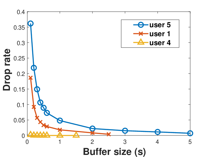
To conclude this section, we look at the impact of channel variability on the required size of the buffer so that the loss of information (dropped packets) is very low. We pick three users with different channel characteristics: user 4 that has the lowest variation of per-block rate (its coefficient of variation is ), user 5 that has the highest variation (), and user 1 with . The network resources are shared equally among all the users, and the other parameters remain unchanged. We choose the (constant) playout rates to be approximately equal to the average of the data rare for each user (that is a reasonable value is expected to keep the drop rates and outages low under large buffers): Mbps, Mbps, and Mbps. We look at what the drop rate will be as a function of the buffer size, where the latter is now expressed in seconds of live video content.
Fig. 7 shows the drop rates for the three users for different buffer sizes. User 4 (with almost constant data rates) requires a very low buffer, where even a s buffer suffices to provide no loss of packets. This helps in preserving low latency (keeping the playout delay on the user’s side of only s). As the variability in the channel conditions increases, the size of the required buffered content increases; a buffer of s is needed to yield a drop rate lower than . Finally, for user 5, a buffer of slightly larger than s is needed to result in a drop rate lower than . This result is particularly important as it shows that for channel conditions with a coefficient of variation up to the latency on the user’s side of less than s is guaranteed with almost no information loss.
| User | 1 | 2 | 3 | 4 | 5 | 6 | 7 | 8 |
|---|---|---|---|---|---|---|---|---|
| (Sc.1) | 0.06 | 0.05 | 0.04 | 0.04 | 0.06 | 0.05 | 0.05 | 0.04 |
| (Sc.2) | 0.06 | 0.05 | 0.04 | 0.04 | 0.11 | 0.1 | 0.09 | 0.04 |
| (Sc.3) | 0.11 | 0.12 | 0.08 | 0.08 | 0.15 | 0.13 | 0.12 | 0.06 |
| (Sc.1) | 0.05 | 0.02 | 0.04 | 0.02 | 0.02 | 0.02 | 0.02 | 0.11 |
| (Sc.2) | 0.04 | 0.02 | 0.09 | 0.02 | 0.13 | 0.08 | 0.12 | 0.15 |
| (Sc.3) | 0.03 | 0.02 | 0.1 | 0.02 | 0.11 | 0.07 | 0.11 | 0.17 |
7 Related work
In general, there isn’t a significant body of research dealing with resource allocation for real-time video streaming in cellular networks, especially not papers containing an analytical framework in a 5G context. Most of the works are constrained with non-live video streaming, such as [26] that deals with buffer dimensioning, [27] that is a system-related paper allowing varying playout rates, or [28] that presents an approach for predicting user’s QoE.
Network slicing as a new concept in 5G has been proposed in [29] to enhance the video streaming experience in vehicular networks. The objective function combines several variables of interest. However, the playout rate is allowed to change, which deteriorates the QoE. Also, the approach in [29] is not applicable to live video streaming.
Optimizing social welfare when streaming in real time in a mobile edge computing framework is the focus of [30]. The considered metric is a special-case expression for QoE. Auctions are used to obtain the optimal solution that is not in closed-form. On the other hand, in our work we provide closed-form expressions (whenever possible) corresponding to other objective functions than in [30].
In [31], a system, called Jigsaw, for 4K real-time video streaming is presented. While Jigsaw indeed provides a superior performance, it operates on 60 GHz frequencies, whereas our system operates in the sub-6 GHz band. Therefore, an adequate comparison between the two approaches is not feasible. Furthermore, there is no theoretical analysis in [31].
The related works most in spirit to ours are [9] and [32]. The possibility of having a constant data rate that can be translated into a constant playout rate has been analyzed in [9], and the reallocation of unused resources to the same users can further improve the QoE. However, as is shown here, providing constant data rates leads to inefficient use of resources. On a similar note, in [32] the authors present a framework that relies on the Brownian approximation to optimize the QoE in terms of the playback latency and video interruptions for live streaming. A policy that jointly determines the amount of playback latency of every user and the scheduling decision of each packet transmission is proposed. It is worth noting that in our paper we follow a different approach, have different setup and objectives. The assumption in [32] is that in a frame only one packet can be transmitted to at most one user. This is unrealistic because in 5G the frame duration is ms, which implies that a considerable number of packets can be forwarded. Another simplified assumption in [32] is that all the links exhibit similar reliability (corresponding to identical per-block rates), while we consider heterogeneous users.
In [20], the authors mimic the operation of DASH by introducing two levels (minimum, maximum) related to the operation of the playout buffer, and based on that determine the playout rate. On the other hand, [21], [33], provide different QoE metrics while assuming that the playout rate is variable. However, in this paper, we show that for several combinations of these 2-level values from [20], our approach provides higher QoE (for any of its definitions in [21], [33]) than the adaptive playout approach.
8 Conclusion
In this paper, we have considered analytically the problem of resource allocation to improve the QoE of cellular users with real-time video streaming, where users have finite-size buffers. We have solved three problems yielding the corresponding best policies. The analysis is validated on trace data. We have compared the corresponding optimal policies against other benchmarks, for different QoE metrics. Results show that the performance can be improved significantly with the proper resource allocation. In the future, we plan to consider resource allocation for other objectives.
References
- [1] “5G vision and requirements,” 2014, white paper.
- [2] M. S. Elbamby, C. Perfecto, M. Bennis, and K. Doppler, “Toward low-latency and ultra-reliable virtual reality,” IEEE Network, vol. 32, no. 2, 2018.
- [3] Nokia, “5G radio access: System design aspects,” www.networks.nokia.com/file/37611/5g-radio-access, 2015, white paper.
- [4] Y. Qi, M. Hunukumbure, M. Nekovee, J. Lorca, and V. Sgardoni, “Quantifying data rate and bandwidth requirements for immersive 5G experience,” in Proc. of IEEE ICC Workshop on 5G RAN Design, 2016.
- [5] S. E. Elayoubi, S. B. Jemaa, Z. Altman, and A. Galindo-Serrano, “5G RAN slicing for verticals: Enablers and challenges,” IEEE Comm. Magazine, vol. 57, no. 1, 2019.
- [6] H. Nam, K. Kim, and H. Schulzrinne, “QoE matters more than QoS: Why people stop watching cat videos,” in Proc. of IEEE INFOCOM, 2016.
- [7] https://mux.com/blog/how-do-users-feel-about-video-streaming-quality-on-their-tvs.
- [8] “5G radio access,” www.ericsson.com/res/docs/whitepapers/wp-5g.pdf, 2016, Ericsson white paper, Uen 284 23-3204 C.
- [9] F. Mehmeti and C. Rosenberg, “How expensive is consistency? Performance analysis of consistent rate provisioning to mobile users in cellular networks,” IEEE Transactions on Mobile Computing, vol. 18, no. 5, 2019.
- [10] R. Trivisonno, R. Guerzoni, I. Vaishnavi, and D. Soldani, “Towards zero latency software defined 5G networks,” in Proc. of IEEE ICCW, 2015.
- [11] A. Gupta and J. R. Kumar, “A survey of 5G network: Architecture and emerging technologies,” IEEE Access, vol. 3, 2015.
- [12] G. Ku and J. M. Walsh, “Resource allocation and link adaptation in LTE and LTE Advanced: A tutorial,” IEEE Communications Surveys & Tutorials, vol. 17, no. 3, 2015.
- [13] ETSI, “5G NR overall description: 3GPP TS 38.300 version 15.3.1 release 15,” www.etsi.org, 2018, technical specification.
- [14] D. Kim, B. C. Jung, H. Lee, D. K. Sung, and H. Yoon, “Optimal modulation and coding scheme selection in cellular networks with hybrid-ARQ error control,” IEEE Transactions on Wireless Communications, vol. 7, no. 12, 2008.
- [15] X. Chen, T. Tan, and G. Cao, “Energy-aware and context-aware video streaming on smartphones,” in Proc. of IEEE ICDCS, 2019.
- [16] S. Sengupta, V. K. Yadav, Y. Saraf, H. Gupta, N. Ganguly, S. Chakraborty, and P. De, “MoviDiff: Enabling service differentiation for mobile video apps,” in Proc. of IFIP/IEEE Symposium on Integrated Network and Service Management (IM), 2017.
- [17] C. Bisdikian, J. S. Lew, and A. N. Tantawi, “The generalized D[X]/D/1 queue: A flexible computer communications model,” Telecommunication Systems, vol. 6, no. 1, 1996.
- [18] P. V. Mieghem, Performance analysis of communication networks and systems. Cambridge University Press, 2006.
- [19] A. Oppenheim and A. Willsky, Signals and systems. Prentice Hall, 1996.
- [20] Y. Xu, Y. Zhou, and D. Chiu, “Analytical QoE models for bit-rate switching in dynamic adaptive streaming systems,” IEEE Trans. on Mob. Comp., vol. 13, no. 12, 2014.
- [21] V. Joseph and G. de Veciana, “NOVA: QoE-driven optimization of DASH-based video delivery in networks,” in Proc. of IEEE INFOCOM, 2014.
- [22] https://zenodo.org/record/1220256#.XiZbo8hKhPY.
- [23] B. Meixner, J. W. Kleinrouweler, and P. Cesar, “4G/LTE channel quality reference signal trace data set,” in Proc. of ACM MMSys, 2018.
- [24] B. Cells, “Baicells technical training,” https://baicells.zendesk.com/hc/en-us/articles/115003137453-WISPAPALOOZA-2017-Technical-Training-Slides, 2017, tech report.
- [25] A. Samuylov, D. Moltchanov, R. Kovalchukov, R. Pirmagomedov, Y. Gaidamaka, S. Andreev, Y. Koucheryavy, and K. Samouylov, “Characterizing resource allocation trade-offs in 5G NR serving multicast and unicast traffic,” IEEE Transactions on Wireless Communications, vol. 19, no. 5, 2020.
- [26] T. Hoßfeld, C. Moldovan, and C. Schwartz, “To each according to his needs: Dimensioning video buffer for specific user profiles and behavior,” in Proc. of IFIP/IEEE International Symposium on Integrated Network Management (IM), 2015.
- [27] T. Y. Huang, R. Johari, N. McKeown, M. Trunnell, and M. Watson, “A buffer-based approach to rate adaptation: Evidence from a large video streaming service,” SIGCOMM Comput. Commun. Rev., vol. 44, no. 4, 2014.
- [28] U. Bulkan and T. Dagiulkas, “Predicting Quality of Experience for online video service provisioning,” Multimedia Tools and Applications, no. 78, 2019.
- [29] H. Khan, S. Samarakoon, and M. Bennis, “Enhancing video streaming in vehicular networks via resource slicing,” IEEE Trans. on Vehicular Technology, vol. 69, no. 4, 2020.
- [30] Y. Hung, C. Wang, and R. Hwang, “Optimizing social welfare of live video streaming services in mobile edge computing,” IEEE Trans. on Mob. Comp., vol. 19, no. 4, 2020.
- [31] G. Baig, J. He, M. A. Qureshi, L. Qiu, G. Chen, P. Chen, and Y. Hu, “Jigsaw: Robust live 4K video streaming,” in Proc. of ACM MobiCom, 2019.
- [32] P.-C. Hsieh, X. Liu, and I.-H. Hou, “Fresher content or smoother playback? A Brownian-approximation framework for scheduling real-time wireless video streams,” in Proc. of ACM Mobihoc, 2020.
- [33] X. Chen, T. Tan, and G. Cao, “Energy-aware and context-aware video streaming on smartphones,” in Proc. of IEEE ICDCS, 2019.