Fair for All: Best-effort Fairness Guarantees for Classification
Abstract
Standard approaches to group-based notions of fairness, such as parity and equalized odds, try to equalize absolute measures of performance across known groups (based on race, gender, etc.). Consequently, a group that is inherently harder to classify may hold back the performance on other groups; and no guarantees can be provided for unforeseen groups. Instead, we propose a fairness notion whose guarantee, on each group in a class , is relative to the performance of the best classifier on . We apply this notion to broad classes of groups, in particular, where (a) consists of all possible groups (subsets) in the data, and (b) is more streamlined.
For the first setting, which is akin to groups being completely unknown, we devise the PF (Proportional Fairness) classifier, which guarantees, on any possible group , an accuracy that is proportional to that of the optimal classifier for , scaled by the relative size of in the data set. Due to including all possible groups, some of which could be too complex to be relevant, the worst-case theoretical guarantees here have to be proportionally weaker for smaller subsets.
For the second setting, we devise the BeFair (Best-effort Fair) framework which seeks an accuracy, on every , which approximates that of the optimal classifier on , independent of the size of . Aiming for such a guarantee results in a non-convex problem, and we design novel techniques to get around this difficulty when is the set of linear hypotheses. We test our algorithms on real-world data sets, and present interesting comparative insights on their performance.
1 Introduction
Machine learning is playing an ever-increasing role in making decisions that have a significant impact on our lives. Of late, we have seen the deployment of machine learning methods to provide advice for decisions pertaining to criminal justice (Angwin et al., 2016; Berk et al., 2018), credit/lending (Koren, 2016), health/medicine (Rajkomar et al., 2018), etc. Given the concerns of disparate impact and bias in this regard (Angwin et al., 2016; Barocas and Selbst, 2016), it is imperative that machine learning models are fair.
The question of defining notions of fairness, and developing methods to achieve them, has received a great deal of attention (Barocas et al., 2017; Binns, 2018). A common theme among the many approaches proposed thus far (Kleinberg, 2018; Chouldechova, 2017) is to fix beforehand a list of protected groups, and then ask for the (approximate) equality of some statistical measure across them. For example, parity seeks to equalize the accuracy across the given groups (Calders et al., 2009), while equalized odds seeks to equalize false positive or false negative rates (Hardt et al., 2016).
Classical definitions of fairness from microeconomics have also found application in machine learning (Balcan et al., 2019; Chen et al., 2019b; Hossain et al., 2020). In particular, there has been recent work (Zafar et al., 2017; Ustun et al., 2019) on adapting the notion of envy-freeness, which is born out of fair division theory (Brams and Taylor, 1996), to a group-based variant tailored to (binary) classification – every given pre-defined group should prefer the way it is classified (on aggregate) in comparison to how it would have been if it assumed the identity of some other group.
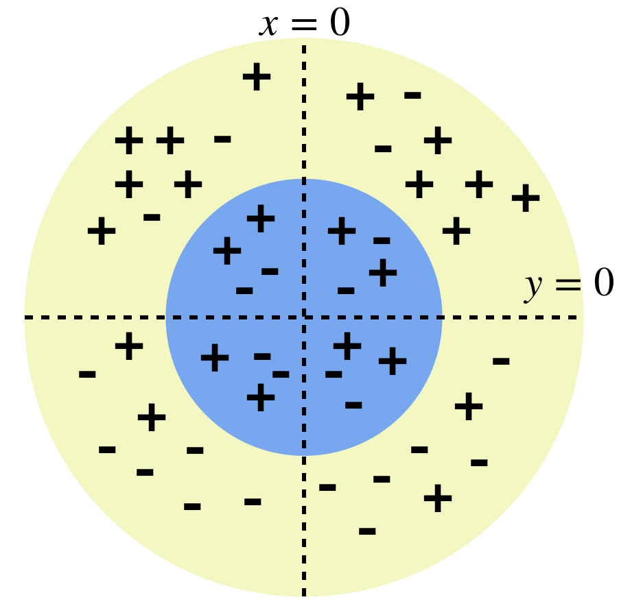
A major drawback of the aforementioned approaches is that they aim for an absolute guarantee: when some of the groups are inherently harder to classify than others, trying to achieve a particular measure of fairness, say equalized odds (Hardt et al., 2016), could do more harm than good by bringing down the accuracy on a group that is easier to classify (see Figure 1 for an example). In this paper, we take a more relative best-effort approach: aiming for guarantees that are defined in terms of how well each group can be classified in itself.
Another drawback of the standard approaches to fairness is that they depend critically on the specification of groups (via sensitive features such as race, gender, etc.). In many cases, the sensitive features are either missing (Chen et al., 2019a), or unusable, considering the need to adhere to treatment parity and anti-discrimination laws (Barocas and Selbst, 2016). Even if they can be used, it is sometimes not clear what the right categorization within them should be. For instance, it could be that a particular demographic group, which is defined on the basis of a shared cultural or ethnic feature, is actually a collection of hidden subgroups that are otherwise quite heterogeneous in terms of other socio-economic indicators (Meier and Melton, 2012; Chang, 2011). Therefore, mis-specifying or mis-calibrating the protected groups could end up hurting some groups within the data, potentially leading to unintended consequences such as a feeling of resentment among them (Hoggett et al., 2013).
We use the following instructive albeit stylized example to illustrate the effect of missing group information.
Example 1.
As shown below in Table 1, there are two binary features , and a hidden demographic feature . The target label follows the formula : if the hidden feature , then is a perfect classifier, and if , then is a perfect classifier. For brevity, we define three groups: , , and .
As a concrete example, suppose each data point corresponds to a job candidate. The hidden feature corresponds to gender, correspond to measures of two different traits, and the assignment to one of two jobs. Suppose the family of available classifiers is . It can be seen that any of these classifiers does poorly in terms of fairness for groups based on the hidden feature .
Consider the classifier (in this case, a solution to the standard Empirical Risk Minimization (ERM) with - loss), which correctly classifies all data except those in . Therefore, the ERM classifier is unfair to those of gender . Our PF classifier (which we shall see later) gets around this issue by randomizing between and . This allows us to classify and correctly with probability , and correctly with probability . Note that the PF classifier is able to treat every gender equally in expectation, even without access to the gender labels.
In order to deal with the above issues, we take a best-effort approach to fairness, one that can be applied to broad classes of groups. If the group identities were well defined and limited in number, simple solutions work: for example, one could perhaps train decoupled classifiers (Ustun et al., 2019; Dwork et al., 2018). With the unavailability or mis-specification of group information, however, the problem is much more interesting. In this regard, we look at two settings – where the groups taken into account are given by (a) all possible subsets in the data, and (b) a more streamlined class of groups, such as all linearly separable ones.
In the former setting, we are effectively reasoning about fairness even though there are no pre-specified groups. Standard statistical notions are of no use in this regard, for, as noted by Kearns et al., 2018, “we cannot insist on any notion of statistical fairness for every subgroup of the population: for example, any imperfect classifier could be accused of being unfair to the subgroup of individuals defined ex-post as the set of individuals it mis-classified.”
In fact, such a limitation also applies to any deterministic classifier. Therefore, focusing on randomized classifiers, the questions we consider first (Section 2) are: What is the best possible best-effort guarantee that can be achieved for all groups simultaneously? We will see that, on account of taking all groups into account, some of which could be too complex to be meaningful in practice, we have to settle for guarantees that are proportionally weaker for smaller subsets. Are there algorithms that achieve such a guarantee? We answer this question in the affirmative by devising the Proportional Fairness (PF) classifier.
The next natural question is: can we do better if we consider a more streamlined class of groups? We will see (Section 3) that this is indeed the case. We note here that standard fairness notions (such as parity) can also be applied in such settings, by effectively solving a convex optimization problem (Kearns et al., 2018). In our best-effort fairness (BeFair) approach, even when we consider linearly separable groups, we need to solve a non-convex problem. A major contribution of our work is devising a way of dealing with this difficulty, and at that, one that works well in practice. In Section 4, we evaluate all our algorithms on real-world datasets. We see that our BeFair approach is able to achieve strong best-effort guarantees, significantly better than standard ERM classifiers. We also present several empirical insights on the performance on PF, mostly in line with our theoretical results.
A more detailed overview of our results are provided in Section 1.2. All our proofs are provided in the Appendix.
1.1 Related literature
The extant literature on fairness in machine learning Hardt et al., 2016; Kamiran and Calders, 2012; Hajian and Domingo-Ferrer, 2012; Chouldechova, 2017; Corbett-Davies et al., 2017 primarily considers statistical notions of fairness which require the protected groups to be specified as input to the (binary) classification problem. Many of these notions are further known to be incompatible with one another Kleinberg, 2018; Friedler et al., 2016. Individual notions of fairness, which loosely translate to asking for “similar individuals” to be “treated similarly”, have also been studied Dwork et al., 2012. However, this requires additional assumptions to be made about the problem at hand, in the form of, e.g., a “similarity metric” defined on pairs of data points. Another related notion is envy-freeness (Hossain et al., 2020), which isn’t very useful without group information (more in the Appendix).
There are several papers on fairness that utilize the broadly applicable framework of minimax optimization in their algorithms (Agarwal et al., 2018; Rezaei et al., 2020; Baharlouei et al., 2019; Madras et al., 2018). For example, Rezaei et al., 2020 derive a novel distributionally robust classification method by incorporating fairness criteria into a worst-case loss minimization program. When compared with this literature, our work is different in one or both of two senses: First, we have a novel and conceptually different notion of fairness that approximates the best-effort guarantee for each group, as opposed to objectives such as max-min fairness or parity. Second, the cardinality of the set of groups can be unbounded (defined by linear constraints on either the feature space or its basis expansion) in our case, as opposed to operating with a fixed set of groups. As we shall see later, each of these aspects presents its own technical challenges.
Several issues have been raised with respect to defining the demographic groups that need to be considered for fairness. Chen et al., 2019a assess the prevalence of disparity when missing demographic identities are imputed from the data. Hashimoto et al., 2018 look at a model where user retention among different groups is linked to the accuracy achieved on them respectively, and design algorithms that improve the user retention among minority groups based on distributionally robust optimization. Their methods, while oblivious to the identity of the groups, operate under the assumption that there are a fixed number of groups, and work well in practice for small . (Kim et al., 2019) develop multi-accuracy auditing to guarantee the fairness for identifiable subgroups, by post-processing the classifier such that it is unbiased. Kearns et al., 2018 study the problem of auditing classifiers for statistical parity (or other related fairness concepts) across a (possibly infinite) collection of groups of bounded VC dimension. However, they do not consider the fact that some groups could be inherently harder to classify than others, and instead work with standard statistical notions such as statistical parity. Doing so results in a non-convex problem – something that we deal with in our work.
Our BeFair approach assumes black-box access to an agnostic learning oracle. Such reductions are commonplace in recent work on fairness in machine learning (Kearns et al., 2018). For example, Agarwal et al., 2018 reduce fair classification to a sequence of cost-sensitive classifications, the solutions of which can be achieved using out-of-the-box classification methods.
The study of fairness has had a much longer history in economics, in particular, the literature on fair division and cake-cutting (Brams and Taylor, 1996; Robertson and Webb, 1998). Out of this line of work have emerged general notions of fairness such as proportionality (Steinhaus, 1948), envy-freeness (Varian, 1974), the core (Foley, 1970), and egalitarian (or maxmin) fairness (Rawls, 2009; Hahne, 1991), to name a few. Of these, the idea of envy-freeness has received great attention in computer science (e.g., (Chen et al., 2013; Cohler et al., 2011)), and been amenable to adaptation into machine learning as a group-based notion of fairness (Balcan et al., 2019; Ustun et al., 2019; Zafar et al., 2017). Hossain et al., 2020 devise algorithms, for multi-class classification that can achieve a variant of group-based (approximate) envy-freeness, with sample complexity of the order of , where is the collection of pre-defined groups. Our guarantees on the accuracy of the PF classifier are related to the notion of the core: for example, analogous guarantees have been studied in the setting of participatory budgeting (Fain et al., 2016). However, dealing with envy-freeness at an individual level, in the absence of group information, is not very useful. Even in simple binary settings, such as loan and bail applications (all individuals prefer being classified positively, i.e. receiving a loan/bail), satisfying envy-freeness requires all individuals to receive the same outcome (Hossain et al., 2020).
Practical implementations of the above-mentioned economic notions of fairness have garnered interest in the literature on network resource allocation (Kleinberg et al., 1999; Kumar and Kleinberg, 2006). Proportional fairness (Kelly et al., 1998; Bonald et al., 2006) has been seen as a way of attaining a middle-ground between welfare maximization and maxmin fairness (Jain et al., 1984). The applicability of proportional fairness to machine learning, in terms of the performance of classification across groups, has, to the best of our knowledge, not been studied before. Although, Li et al., 2019 do study fair resource allocation based on -fairness (of which proportional fairness is a special case with ) to improve fairness in terms of the performance across devices in a decentralized federated learning setting.
1.2 Our model and results
We are given a set of data points denoted by , with their features given by , and their true binary labels by . The hypothesis space at hand will be denoted by , a set of (deterministic) classifiers. The Boolean variable denotes whether the classifier correctly classifies data point . In other words, . A classification instance is defined by a pair . We assume that for any classifier , its complement , defined by flipping the classification outcomes of (i.e., ), is also in . This assumption is valid for most natural families of binary classifiers. We denote by the space of all randomized classifiers over . If is obtained via a distribution over , then for a data point , we defined the utility .
We are given , a class of groups, each element of which is of the form . means is in the group and indicates the opposite. We also use to denote the subset given by and as its size . For any such , its utility under is .
For each , define to be the best classifier for the group . The best-effort fairness guarantee is captured via a constraint of the form . The function constrains the accuracy of , the classifier at hand, to that of the optimal classifier for , with a possible dependence on the size of the group . Applying such a constraint for all gives us a uniform best-effort fairness guarantee. What sort of is workable depends on the class considered.
In Section 2, we consider the case where includes all the subsets of , i.e., there is no specific information about . Via a theoretical worst-case bound (Theorem 1), we show that the best we can do in this case is to choose . For any group that can be perfectly classified by some (), the same constraint boils down to : in other words, a utility of at least should be guaranteed on such a set. Such a guarantee can be interpreted as fairness: If is a potentially hidden demographic that can be perfectly classified using some features, our classifier should not ignore those features entirely. We show that our PF classifier in fact achieves this guarantee (Theorem 2).
In Section 3, we consider a more streamlined class of groups: in particular, contains all linearly separable groups. For ease of exposition, we define the error , and recast the discussion in terms of it.11 1 While a fundamentally similar discussion can be done in terms of the utilities, using errors instead leads to an easier handling of the constants involved. In this case, we seek a much stronger guarantee: . The general form of the optimization problem we solve is as follows:
As discussed in more detail later, to solve the above problem we need to deal with the non-convex constraints. We outline a method (BeFair) to do so when consists of linearly separable groups. We will also look for a slightly weaker guarantee as follows: , for some – weaker because now has a slightly larger target to approximate. Our techniques extend seamlessly to such a formulation also.
2 Best-effort guarantee for all groups
The first question to ask is whether there is a fundamental limit on how well one can hope to do with respect to fairness in the setting where . Since we are dealing with a notion of fairness that is measured relative to the family of classifiers at hand, we first want to understand what the best guarantee that can be given is (in the form of a worst-case bound), with no conditions on the type of classifiers used.
Theorem 1.
On any data set , there is no randomized classifier (for some ) such that for all admitting a perfect classifier (i.e., ), we have .
This theorem shows that, in terms of how much utility is accrued by each of the perfectly classified sets, the best bound we can hope to target is one proportional to the fractional size of the given set of data points. Note that for every instance, there exists some , such that the claim of the theorem holds – this is not true more generally in the sense that there could exist some for which the claim does not hold as shown by Example 2 (in the Appendix).
2.1 Proportional Fairness (PF) Classifier
We now demonstrate a classifier that matches the above bound as long as the utilities ’s are binary (which holds in our model, but could also be encountered in other scenarios involving resource allocation discussed in Section 1.1); as mentioned before, this captures multi-class classification as well. The Proportional Fairness classifier is defined as follows:
Definition 1 (Proportional Fairness (PF)).
Given an instance , the PF classifier is the one that maximizes over all .
As mentioned before, the proportional fairness objective has had a long history in network resource allocation literature (Kelly et al., 1998). However, to the best of our knowledge, its applicability to the classification problem, and the implications thereof, have never been established before.
We now show that the PF classifier achieves a guarantee matching the worst-case bound in Theorem 1.
Theorem 2.
For any subset that admits a perfect classifier (i.e., ) we have .
Thus, the PF classifier achieves, on any subset, an accuracy that is proportional to the accuracy of the best classifier on that subset scaled by the fractional size of the subset. As mentioned earlier, the use of perfectly classifiable subsets in our analysis is just for the ease of exposition. The results can be suitably translated to using all possible subsets. For example, the following is a simple corollary of Theorem 2:
Corollary 2.1.
For any subset , with its best classifier , we have , where .
Assuming black-box access to an agnostic learning oracle, the PF classifier can be computed using a primal dual style algorithm (details in the Appendix, or see Bhalgat et al., 2013 for similar results). In our experiments, we just use a heuristic instead (see Section 4, and also the Appendix). We also do not explicitly discuss the generalization properties – but we would expect that PF is not prone to overfitting, since all possible groups have to be given a guarantee on performance (details in the Appendix).
Interpreting the results:
Theorem 2 and Corollary 2.1 neatly characterize how PF achieves the best possible theoretical bound . One drawback of applying PF in practice is that the theoretical guarantee is proportionally lower for smaller groups, notwithstanding the fact that, in practice, the accuracy of PF on small groups is much better than what is given by these bounds (see Section 4). As far as the bounds as concerned, the reason that we have to settle for an accuracy proportionally lower for smaller subsets is that the guarantee has to hold for all possible subsets. Some of these subsets could be extremely complex, and possibly unreasonable in most practical settings. As will see next, we can do much better with more restricted classes of groups.
3 Best-effort guarantees for linearly separable groups
In this section, we limit to be a more streamlined class of groups, and aim for a much stronger guarantee. We then devise an algorithm that achieves such a guarantee. As mentioned in Section 1.2, we want to find a a randomized classifier that, for every group , achieves an absolute error which is within an additive factor from that of the optimal classifier for . In particular, the optimization problem we would like to solve is the following:
Problem 1 (BeFair).
For a given hypothesis space , a class of groups , and ,
In particular, we consider to be the space of linear hypotheses, and the class of all linearly separable groups.22 2 If , then and are linearly separable. As mentioned earlier, despite using linear hypotheses and groups, we are faced with a non-convex problem. It can be seen that the non-convexity stems from the best-effort constraint – while the terms and can be individually made convex by using standard surrogate loss functions, their combination obtained by subtracting one from the other cannot. Note that such a difficulty does not arise for the more absolute notions of fairness such as parity, as is the case with the techniques in Kearns et al., 2018. Also, even in our setting, if were a small finite set, then all the optimal classifiers could be calculated offline, and the corresponding constraints listed to form a simpler convex optimization problem.
We redefine the BeFair() as follows to explicitly factor the hidden optimization problem of finding into the corresponding constraint for ; by using the fact that if , then for any .
Problem 2 (BeFair).
We first define the partial Lagrangian corresponding to Problem 2. Let . With dual variables for every and :
In order to have a convergent algorithm for our optimization, we will restrict the dual space to the bounded set , where will be a parameter in our algorithm. Then, by the Minimax Theorem, solving Problem 2 is equivalent to solving the following:
| (1) |
The minmax problem can be viewed as a two player zero-sum game: The set of pure strategies for the learner (corresponding to the primal) corresponds to – each deterministic classifier is a valid pure strategy. For the adversary (corresponding to the dual), the pure strategies in can be either the all zeros vectors, or a particular choice of . Then, solving Problem 2, via the minmax formulation in Equation 1, is the same as finding an equilibrium of the corresponding two-player zero-sum game with as the payoff for the dual player.
3.1 Solving the BeFair() problem via a convex relaxation:
The equilibrium of a two-player zero-sum game can be found using Fictitious Play, an iterative algorithm which is guaranteed to converge33 3 The asymptotic convergence is usually fast in practice, and especially so in our experiments. given that we can solve for the best responses of both players (Robinson, 1951). Fictitious Play (Brown, 1949) proceeds in rounds alternating between the primal and dual player: in each round, each player chooses a best response to the the mixed strategy that randomizes uniformly over the empirical history of the other’s strategies. A formal description is given in Algorithm 1.
Learner’s best response:
For a given mixed strategy of the adversary, the learner needs to solve:
Since the optimum is obtained at the corner points of the feasible region of the strategy space, we need only consider pure strategies for the optimization problem above. The learner’s problem then becomes:
where , and this can be solved since we assume black-box access to a weighted ERM oracle. In practice, many heuristics (like Logistic Regression, Boosting, etc.) are used effectively for this problem, even though it is known to be hard in the worst case (Feldman et al., 2012).
Adversary’s best response:
The adversary’s best response problem is more involved and will require some novel techniques to solve. Again, we need to optimize only over pure strategies. With a bit of analysis, the dual best response problem can be seen to be equivalent to solving, for a given :
| (2) |
For all , define . Then the above objective can be written as
| (3) |
which is non-convex. For each , we would like to convexify it differently when or . (The convex relaxations are not exact.)
Since we only consider the case where both and consist of linear hypotheses, define and , where and are the coefficients of the linear hypotheses and respectively.
For each , we add the term to the objective. The first term, , is treated as ; and the second term, , is replaced by , whence the whole objective becomes , which is convex.
Therefore, we need to solve
| (4) |
which can be done via convex optimization methods.
The solution returned by Algorithm 1 has to be checked for feasibility with respect to Problem 2 – this tells us if the problem is feasible to begin with. Also, the solution to the Adversary’s problem (Equation 2) can potentially be improved by alternately optimizing for and , à la Expectation-Maximization: For a fixed , we can optimize by using Equation 3.1 and a convexification analogous to Equation 4. The converse problem of optimizing , for a fixed , is just a weighted ERM problem.
Note that our technique works as is even for groups that can be defined in terms of any basis expansion of a limited size (a commonly used way of capturing non-linear relationships with linear methods). For example, if there are two numerical features , then by encoding the values as additional features, we can solve the problem over all groups defined via conic sections (in the feature space). Similarly, a Boolean AND of binary features can also be written as a linear constraint: for binary features taking values in , is equivalent to . Extensions to more general classes of and are an interesting open problem.
3.2 A more general version of BeFair():
For , we can generalize Problem 2 as follows:
Problem 3 (-BeFair).
The only difference from Problem 2 is that we have slightly weaker constraints: the error of on is compared with times the least possible error on . With a straightforward modification, the overall technique in Section 3.1 works for this problem too.
For a fixed , computing the quantity gives us a way of measuring the fidelity of any given classifier . To do so, the Adversary’s problem can be solved (as shown) to find the smallest for which becomes feasible for the constraints in Problem 3 (i.e., satisfies the best-effort guarantees). We discuss this in more detail in Section 4.1.
4 Experiments
The primary goal of our experiments is to show that the BeFair algorithm works extremely well in practice. As we discuss below, BeFair achieves its intended purpose (as discussed in the previous section), by achieving strong best-effort fairness guarantees uniformly over all linearly separable groups. In particular, it is able to achieve a performance that is a close approximation of the best possible on these groups (as given in Problem 3) for small values of and . In addition, we will also evaluate the PF algorithm and show how it behaves differently from BeFair, on account on having to provide guarantees for all possible groups, even those corresponding to a high VC dimension. We also show how, in practice, the performance of PF seems to be better than what is suggested by the worst-case lower bound via Theorem 2 (which is proportionally weaker for smaller groups).
We work with two data sets: adult, the Adult44 4 48842 instances, 14 features, https://archive.ics.uci.edu/ml/datasets/Adult dataset from the UCI Machine Learning Repository, and compas, the COMPAS55 5 6172 instances, 8 features, https://www.propublica.org/article/how-we-analyzed-the-compas-recidivism-algorithm Risk of Recidivism data set (Angwin et al., 2016). Both have binary labels and a mixture of numerical and categorical features. Using these data sets, we compare and contrast the following methods (recalling their definitions from earlier):
- 1.
PF: As the exact solution of PF is computationally inefficient, we use hPF, a heuristic (details in the Appendix) inspired by Reweighted Approval Voting. (Aziz et al., 2017). In what follows, we refer to hPF as PF.
- 2.
-BeFair as described in Section 3.
- 3.
ERM methods: We use LR (Logisitic Regression), since it performs best here. We also compare overall accuracy with Ada (AdaBoost), an ensemble method.
- 4.
The lower bound given by Corollary 2.1.
| LR | Ada | hPF | -BeFair | -BeFair | |
|---|---|---|---|---|---|
| adult | 0.83 | 0.84 | 0.78 | 0.79 | 0.80 |
| compas | 0.75 | 0.75 | 0.64 | 0.70 | 0.71 |
In Table 2, we present the overall accuracy of various methods, i.e., that measured on the entire test set. As there is a trade-off between ensuring fairness for groups and maximizing overall accuracy, PF has a lower overall accuracy compared to other methods. -BeFair is much closer to the ERM baselines (especially as seen on the compas dataset, even for a small value of . Larger values of can only increase accuracy as the fairness constraints become laxer.
4.1 Evaluating the performance of BeFair
We first define Maximum Additive Error (), parametrized by , of any given classifier .
Definition 2 ().
For a given , and , .
For a given , specifies, for the worst-off group , how much difference there is between the error of and that of the best classifier for scaled by .
For instance, can be computed by searching over different values of to pick the smallest that gives a feasible solution for the -BeFair() problem. On the other hand, can be computed by solving the Adversary’s problem (Equation 3.1 modified as per ) for .
In Figure 2, we compare of ERM and BeFair for . Errors are reported as a percentage of the entire data set.


Many key observations can be made from this plot:
- (a)
As we increase , the of both ERM and BeFair decrease. This is because the best-effort constraints get laxer with increasing .
- (b)
Even for , BeFair achieves an improvement over ERM of close to 50% (since is about half of ) on compas, and 33% on adult, in the value.
- (c)
For a slightly larger value of , we get an extremely low value for of around , which means BeFair gets a strong approximation. Therefore, BeFair is able to achieve an multiplicative error of , with an additive error of around %.
- (d)
decreases linearly with , while most of the improvement in comes from increasing from to . In other words, BeFair is able to extract a bigger improvement with a small increase of .
Overall, BeFair achieves low for small values of .
4.2 Comparison of PF with BeFair:
In Figure 3, we order (on the axis) the data points in the test set in ascending order of their scores (i.e., confidence of predicting the true label) given by LR. For each point , the axis shows the accuracy of various methods on the subset consisting of all points from through . If we imagine the LR scores as a measure of how easy the points are to classify correctly: then we see that PF gets a more uniform error on all these sets, whereas -BeFair has lower error on sets with higher LR scores. This is because the groups where BeFair has high error are probably too complex to be meaningful practically. On the other hand, PF must provide uniform guarantees over all groups, even those corresponding to large VC dimensions, and therefore has a uniformly higher error on them.

4.3 Comparison of PF with the theoretical lower bound
In Figure 4 (left), we order (on the axis) the data points in the test set in ascending order of their scores (i.e., confidence of predicting the true label) given by Ada. For each point , the axis shows the accuracy of various methods on the subset consisting of all points from through . Figure 4 (right) does the same with PF scores.
We see that the accuracy of PF is much higher than the worst-case lower bound. PF comes close to the lower bound for larger subsets, especially for those that are easy to classify (see the Appendix for more details). Note that the lower bound is not monotonic because it depends on both the size of the subset and the best possible classification accuracy on it (Corollary 2.1). Also, in Figure 4 (right), ERM methods do worse because the points with low hPF scores are inherently much harder to classify.


5 Conclusions
In this paper, we study group fairness in the (multi-class) classification setting. We propose a notion based on best-effort guarantees, which requires each group in a class to have a classification accuracy that is as close as possible to the optimal for that group. When consists of all possible groups, we show that PF achieves the theoretical optimum in our setting. When consists of linearly separable groups, we can do much better via the BeFair algorithm, which crucially depends on convexification techniques to solve an essentially non-convex problem. We also test our methods on real-world datasets and show that they perform well in practice, especially the BeFair method.
One interesting question for future work is to extend our techniques for more involved classes of groups, say, for example, when consists of all groups that can be identified by a fixed neural network. Similar extensions of the hypothesis space are also worth looking at. Moreover, in some applications (bail/loan decisions, college admissions, etc.), false negatives and false positives play drastically different roles. Can our framework be extended to deal with such considerations? Can it also be extended to multi-class classification? Note that the guarantees of PF carry over to this setting directly. We would also like to point out that randomized classifiers are not always desirable and have some limitations in practice (Cotter et al., 2019). How to think about best-effort fairness of deterministic classifiers with unknown groups is another interesting open question.
Acknowledgments
This work is supported by NSF grant CCF-1637397, ONR award N00014-19-1-2268, and DARPA award FA8650-18-C-7880. Part of this work was done while Yu Cheng was visiting the Institute of Advanced Study.
References
- Agarwal et al., (2018) Agarwal, A., Beygelzimer, A., Dudík, M., Langford, J., and Wallach, H. M. (2018). A reductions approach to fair classification. In Proceedings of the 35th International Conference on Machine Learning, pages 60–69.
- Angwin et al., (2016) Angwin, J., Larson, J., Mattu, S., and Kirchner, L. (2016). Machine bias. ProPublica, May, 23:2016.
- Arora et al., (2012) Arora, S., Hazan, E., and Kale, S. (2012). The multiplicative weights update method: a meta-algorithm and applications. Theory of Computing, 8(1):121–164.
- Aziz et al., (2017) Aziz, H., Brill, M., Conitzer, V., Elkind, E., Freeman, R., and Walsh, T. (2017). Justified representation in approval-based committee voting. Social Choice and Welfare, 48(2):461–485.
- Baharlouei et al., (2019) Baharlouei, S., Nouiehed, M., Beirami, A., and Razaviyayn, M. (2019). Rényi fair inference. In International Conference on Learning Representations.
- Balcan et al., (2019) Balcan, M.-F. F., Dick, T., Noothigattu, R., and Procaccia, A. D. (2019). Envy-free classification. In Advances in Neural Information Processing Systems, pages 1238–1248.
- Barocas et al., (2017) Barocas, S., Hardt, M., and Narayanan, A. (2017). Fairness in machine learning. NIPS Tutorial.
- Barocas and Selbst, (2016) Barocas, S. and Selbst, A. D. (2016). Big data’s disparate impact. Calif. L. Rev., 104:671.
- Bartlett and Mendelson, (2002) Bartlett, P. L. and Mendelson, S. (2002). Rademacher and gaussian complexities: Risk bounds and structural results. Journal of Machine Learning Research, 3(Nov):463–482.
- Berk et al., (2018) Berk, R., Heidari, H., Jabbari, S., Kearns, M., and Roth, A. (2018). Fairness in criminal justice risk assessments: The state of the art. Sociological Methods & Research, page 0049124118782533.
- Bhalgat et al., (2013) Bhalgat, A., Gollapudi, S., and Munagala, K. (2013). Optimal auctions via the multiplicative weight method. In Proceedings of the fourteenth ACM conference on Electronic commerce, pages 73–90.
- Binns, (2018) Binns, R. (2018). Fairness in machine learning: Lessons from political philosophy. In Conference on Fairness, Accountability and Transparency, pages 149–159.
- Bonald et al., (2006) Bonald, T., Massoulié, L., Proutiere, A., and Virtamo, J. (2006). A queueing analysis of max-min fairness, proportional fairness and balanced fairness. Queueing systems, 53(1-2):65–84.
- Brams and Kilgour, (2014) Brams, S. J. and Kilgour, D. M. (2014). Satisfaction approval voting. In Voting Power and Procedures, pages 323–346. Springer.
- Brams and Taylor, (1996) Brams, S. J. and Taylor, A. D. (1996). Fair Division: From cake-cutting to dispute resolution. Cambridge University Press.
- Brown, (1949) Brown, G. W. (1949). Some Notes on Computation of Games Solutions. RAND Corporation, Santa Monica, CA.
- Calders et al., (2009) Calders, T., Kamiran, F., and Pechenizkiy, M. (2009). Building classifiers with independency constraints. In 2009 IEEE International Conference on Data Mining Workshops, pages 13–18. IEEE.
- Chang, (2011) Chang, T. (2011). Debunking the myth of ’homogeneous’ asian students. https://www.educationworld.com/a_admin/debunking_myth_of_homogeneous_asian_students.shtml.
- (19) Chen, J., Kallus, N., Mao, X., Svacha, G., and Udell, M. (2019a). Fairness under unawareness: Assessing disparity when protected class is unobserved. In Proceedings of the Conference on Fairness, Accountability, and Transparency, pages 339–348.
- (20) Chen, X., Fain, B., Lyu, L., and Munagala, K. (2019b). Proportionally fair clustering. In Proceedings of the 36th International Conference on Machine Learning, pages 1032–1041.
- Chen et al., (2013) Chen, Y., Lai, J. K., Parkes, D. C., and Procaccia, A. D. (2013). Truth, justice, and cake cutting. Games and Economic Behavior, 77(1):284–297.
- Chouldechova, (2017) Chouldechova, A. (2017). Fair prediction with disparate impact: A study of bias in recidivism prediction instruments. Big data, 5(2):153–163.
- Cohler et al., (2011) Cohler, Y. J., Lai, J. K., Parkes, D. C., and Procaccia, A. D. (2011). Optimal envy-free cake cutting. In Twenty-Fifth AAAI Conference on Artificial Intelligence.
- Corbett-Davies et al., (2017) Corbett-Davies, S., Pierson, E., Feller, A., Goel, S., and Huq, A. (2017). Algorithmic decision making and the cost of fairness. In Proceedings of the 23rd ACM SIGKDD International Conference on Knowledge Discovery and Data Mining, pages 797–806.
- Cotter et al., (2019) Cotter, A., Gupta, M., and Narasimhan, H. (2019). On making stochastic classifiers deterministic. In Advances in Neural Information Processing Systems, pages 10910–10920.
- Dwork et al., (2012) Dwork, C., Hardt, M., Pitassi, T., Reingold, O., and Zemel, R. (2012). Fairness through awareness. In Proceedings of the 3rd innovations in theoretical computer science conference, pages 214–226.
- Dwork et al., (2018) Dwork, C., Immorlica, N., Kalai, A. T., and Leiserson, M. (2018). Decoupled classifiers for group-fair and efficient machine learning. In Conference on Fairness, Accountability and Transparency, pages 119–133.
- Fain et al., (2016) Fain, B., Goel, A., and Munagala, K. (2016). The core of the participatory budgeting problem. In International Conference on Web and Internet Economics, pages 384–399. Springer.
- Feldman et al., (2012) Feldman, V., Guruswami, V., Raghavendra, P., and Wu, Y. (2012). Agnostic learning of monomials by halfspaces is hard. SIAM Journal on Computing, 41(6):1558–1590.
- Foley, (1970) Foley, D. K. (1970). Lindahl’s solution and the core of an economy with public goods. Econometrica: Journal of the Econometric Society, pages 66–72.
- Friedler et al., (2016) Friedler, S. A., Scheidegger, C., and Venkatasubramanian, S. (2016). On the (im)possibility of fairness. arXiv preprint arXiv:1609.07236.
- Grötschel et al., (1988) Grötschel, M., Lovász, L., and Schrijver, A. (1988). Geometric Algorithms and Combinatorial Optimization, volume 2 of Algorithms and Combinatorics. Springer. Second Edition, 1993.
- Hahne, (1991) Hahne, E. L. (1991). Round-robin scheduling for max-min fairness in data networks. IEEE Journal on Selected Areas in communications, 9(7):1024–1039.
- Hajian and Domingo-Ferrer, (2012) Hajian, S. and Domingo-Ferrer, J. (2012). A methodology for direct and indirect discrimination prevention in data mining. IEEE transactions on knowledge and data engineering, 25(7):1445–1459.
- Hardt et al., (2016) Hardt, M., Price, E., and Srebro, N. (2016). Equality of opportunity in supervised learning. In Advances in neural information processing systems, pages 3315–3323.
- Hashimoto et al., (2018) Hashimoto, T. B., Srivastava, M., Namkoong, H., and Liang, P. (2018). Fairness without demographics in repeated loss minimization. In Proceedings of the 35th International Conference on Machine Learning, pages 1934–1943.
- Hoggett et al., (2013) Hoggett, P., Wilkinson, H., and Beedell, P. (2013). Fairness and the politics of resentment. Journal of Social Policy, 42(3):567–585.
- Hossain et al., (2020) Hossain, S., Mladenovic, A., and Shah, N. (2020). Designing fairly fair classifiers via economic fairness notions. In Proceedings of the 29th International World Wide Web Conference.
- Jain et al., (1984) Jain, R. K., Chiu, D.-M. W., and Hawe, W. R. (1984). A quantitative measure of fairness and discrimination. Eastern Research Laboratory, Digital Equipment Corporation, Hudson, MA.
- Kamiran and Calders, (2012) Kamiran, F. and Calders, T. (2012). Data preprocessing techniques for classification without discrimination. Knowledge and Information Systems, 33(1):1–33.
- Kearns et al., (2018) Kearns, M. J., Neel, S., Roth, A., and Wu, Z. S. (2018). Preventing fairness gerrymandering: Auditing and learning for subgroup fairness. In Proceedings of the 35th International Conference on Machine Learning, pages 2569–2577.
- Kelly et al., (1998) Kelly, F. P., Maulloo, A. K., and Tan, D. K. (1998). Rate control for communication networks: shadow prices, proportional fairness and stability. Journal of the Operational Research society, 49(3):237–252.
- Khachiyan, (1979) Khachiyan, L. G. (1979). A polynomial algorithm in linear programming. In Doklady Akademii Nauk, volume 244, pages 1093–1096. Russian Academy of Sciences.
- Kim et al., (2019) Kim, M. P., Ghorbani, A., and Zou, J. (2019). Multiaccuracy: Black-box post-processing for fairness in classification. In Proceedings of the 2019 AAAI/ACM Conference on AI, Ethics, and Society, pages 247–254.
- Kleinberg, (2018) Kleinberg, J. (2018). Inherent trade-offs in algorithmic fairness. In Abstracts of the 2018 ACM International Conference on Measurement and Modeling of Computer Systems, pages 40–40.
- Kleinberg et al., (1999) Kleinberg, J., Rabani, Y., and Tardos, É. (1999). Fairness in routing and load balancing. In 40th Annual Symposium on Foundations of Computer Science, pages 568–578. IEEE.
- Koren, (2016) Koren, J. R. (2016). What does that web search say about your credit. Los Angeles Times.
- Kumar and Kleinberg, (2006) Kumar, A. and Kleinberg, J. (2006). Fairness measures for resource allocation. SIAM Journal on Computing, 36(3):657–680.
- Li et al., (2019) Li, T., Sanjabi, M., Beirami, A., and Smith, V. (2019). Fair resource allocation in federated learning. In International Conference on Learning Representations.
- Madras et al., (2018) Madras, D., Creager, E., Pitassi, T., and Zemel, R. (2018). Learning adversarially fair and transferable representations. In International Conference on Machine Learning, pages 3384–3393. PMLR.
- Meier and Melton, (2012) Meier, K. J. and Melton, E. K. (2012). Latino heterogeneity and the politics of education: The role of context. Social science quarterly, 93(3):732–749.
- Papadimitriou and Roughgarden, (2008) Papadimitriou, C. H. and Roughgarden, T. (2008). Computing correlated equilibria in multi-player games. Journal of the ACM (JACM), 55(3):1–29.
- Pedregosa et al., (2011) Pedregosa, F., Varoquaux, G., Gramfort, A., Michel, V., Thirion, B., Grisel, O., Blondel, M., Prettenhofer, P., Weiss, R., Dubourg, V., Vanderplas, J., Passos, A., Cournapeau, D., Brucher, M., Perrot, M., and Duchesnay, E. (2011). Scikit-learn: Machine learning in Python. Journal of Machine Learning Research, 12:2825–2830.
- Rajkomar et al., (2018) Rajkomar, A., Hardt, M., Howell, M. D., Corrado, G., and Chin, M. H. (2018). Ensuring fairness in machine learning to advance health equity. Annals of internal medicine, 169(12):866–872.
- Rawls, (2009) Rawls, J. (2009). A theory of justice. Harvard University Press.
- Rezaei et al., (2020) Rezaei, A., Fathony, R., Memarrast, O., and Ziebart, B. (2020). Fairness for robust log loss classification. In Proceedings of the AAAI Conference on Artificial Intelligence, volume 34, pages 5511–5518.
- Robertson and Webb, (1998) Robertson, J. and Webb, W. (1998). Cake-cutting algorithms: Be fair if you can. AK Peters/CRC Press.
- Robinson, (1951) Robinson, J. (1951). An iterative method of solving a game. Annals of Mathematics, 54(2):296–301.
- Shalev-Shwartz and Ben-David, (2014) Shalev-Shwartz, S. and Ben-David, S. (2014). Understanding machine learning: From theory to algorithms. Cambridge university press.
- Steinhaus, (1948) Steinhaus, H. (1948). The problem of fair division. Econometrica.
- Ustun et al., (2019) Ustun, B., Liu, Y., and Parkes, D. (2019). Fairness without harm: Decoupled classifiers with preference guarantees. In International Conference on Machine Learning, pages 6373–6382.
- Varian, (1974) Varian, H. R. (1974). Equity, envy, and efficiency. Journal of Economic Theory, 9(1):63–91.
- Zafar et al., (2017) Zafar, M. B., Valera, I., Rodriguez, M., Gummadi, K., and Weller, A. (2017). From parity to preference-based notions of fairness in classification. In Advances in Neural Information Processing Systems, pages 229–239.
Appendix A Omitted proofs
Proof.
Suppose there are only two classifiers in : classifies set correctly, and (equivalently ) classifies correctly. If an algorithm chooses with probability and with probability , then the average utility on is , and that on is . Clearly, we cannot simultaneously have and . ∎
Proof.
Let be the PF classifier. Thus maximizes . Therefore, for any and any ,
Since the above expression attains its maxima at , we take the derivative with respect to , and evaluate it at , to get:
Define . Rearranging the inequality above, we get , and consequently,
If of size is perfectly classified by , then the above inequality gives
which in turn implies that
Since the arithmetic mean is at least the harmonic mean, we get
Recall Corollary 2.1: See 2.1
Proof.
For any , we have:
Let be the largest subset of that is perfectly classifiable by . By Theorem 2, . Then, we get
Since , the above inequality turns into
Appendix B Omitted examples
In the following example, we see that there are instances where, for some specific , the claim of Theorem 1 does not hold.
Example 2.
Suppose there are three data points , and there are four classifers in . Classifier classifies correctly, and classifies correctly. If a randomized classifier picks and with the same probability , then for all subsets which are perfectly classifiable, i.e., for each of , , , and , the utility is , , , and , respectively. Each of these utilities is greater than the fractional size of the subsets, which does not agree with the claim of Theorem 1.
Appendix C Computing the Proportional Fairness classifier
In this section, we describe how to compute our Proportional Fairness (PF) classifier. We present computational results for two different settings. Lemma 1 states that when the set of deterministic classifiers are given explicitly, we can compute the PF classifiers in polynomial time. Lemma 2 focuses on the case where there are exponentially or infinitely many deterministic classifiers, and shows that the PF classifier can still be computed in polynomial time, assuming that we have black-box access to an agnostic learning oracle.
Recall that is the set of data-points with , is the set of (deterministic) classifiers with , and if the classifier labels the -th data-point correctly, and otherwise.
The PF classifier is a distribution over deterministic classifiers. PF corresponds to the optimal solution to the following mathematical program:
| (5) |
where the variables describes the randomized classifier (which chooses with probability ); and is the utility of the -th data-point under the distribution (i.e., the probability that the -th data-point is classified correctly). Observe that the objective function is monotone in every , so at optimality, we always have , and for every .
Lemma 1.
Given a classification instance with data-points and classifiers, the mathematical program (5) can be solved to precision in time .
Proof.
When and , the mathematical program (5) has variables. The feasible region is given explicitly by a set of linear constraints. Because the objective function is concave in the variables , we can minimize it using the ellipsoid method (Khachiyan, 1979; Grötschel et al., 1988) in time . ∎
In many applications, we often have infinitely many hypotheses in (e.g., all hyperplanes in ). If this is the case, the mathematical program (5) has infinitely many variables, and to solve it, we need to make some assumptions on the structure of .
A commonly used assumption is that there exists an agnostic learning oracle: given a set of weights on the data-points, the oracle returns an optimal classifier subject to these weights. Formally, we assume black-box access to an oracle for the following problem:
Definition 3 (Agnostic Learning).
Fix a set of data-points and a family of classifiers . Given any weights , find a classifier that maximizes the (weighted) average accuracy on . That is, maximizes .
Given such an oracle, there are a few ways in which Problem (5) can be solved theoretically in polynomial time. We first sketch the outline of a multiplicative weights approach: Consider the feasibility version of the problem, where we want to check if there is a feasible solution that gives us an objective value of at least . If we define a region as the set of , where and , that satisfy:
| (6) | ||||
| (7) |
then the problem can be restated as:
This can be solved via the multiplicative weights if we have an efficient oracle for solving the following optimization problem for a given (Bhalgat et al., 2013; Arora et al., 2012):
| maximize | |||
| subject to |
It can be seen that the above devolves into two decoupled problems: The first one is for , which can be solved analytically,
| minimize | |||
| subject to | |||
and the second for , which can be solved with access to an agnostic learning oracle:
| minimize | |||
| subject to | |||
As the next lemma shows, Problem (5) can also be theoretically solved in a more straightforward way using the ellipsoid method.
Lemma 2.
Given a classification instance with data-points and an agnostic learning oracle for the set of classifiers , the mathematical program (5) can be solved to precision in time .
Proof.
We use the “Ellipsoid Against Hope” algorithm proposed in Papadimitriou and Roughgarden, 2008.
Consider the dual of (5):
| (8) |
The dual program (8) has variables and infinitely many constraints. Strong duality holds despite the infinite-dimensionality of (5).
Let denote the optimal value of the primal and dual programs. The dual objective is convex in , so we can add a constraint
| (9) |
and use ellipsoid method to check the feasibility of the dual with this additional constraint. We show a separation oracle exists so we can run the ellipsoid method. For a fixed point , we can verify Constraint (9) directly, and we can use the agnostic learning oracle to check the infinitely many constraints
| (10) |
because it is sufficient to first use the oracle to find some that maximizes , and then check only the -th constraint.
We know the ellipsoid method must conclude infeasibility, because the minimum possible value of the dual is but we are asking for . Let denote the set of classifiers whose corresponding constraints (10) are checked in the execution of the ellipsoid method. Because the ellipsoid only examines the constraints in and concludes infeasibility, we know that if we replace with in the dual program (8), the objective value is still larger than . Moreover, the cardinality of is at most because the ellipsoid method terminates in steps.
It is worth noting that the proof of Lemma 2 continues to hold even if we only have an -approximately optimal agnostic learning oracle.
Appendix D A heuristic for PF
Here we describe a heuristic for PF drawing inspiration from some literature on social choice (voting). Imagine a social choice setting: we have a set of voters and a set of candidates. Each voter has a subset of candidates which she prefers. The goal here is to select a committee of a fixed size , i.e., a subset (), which “satisfies” the voters as much as possible
One method to do so is Proportional Approval Voting (Aziz et al., 2017), or PAV for short. Here, a voter is assumed (for the sake of computation) to derive a utility of from a committee that contains exactly of her approved candidates, i.e., . For PAV, as a method of computing a committee , the overall goal is to maximize the sum of the voters’ utilities – in other words, PAV outputs a set .
Reweighted Approval Voting (RAV for short) converts PAV into a multi-round rule as follows: Start by setting . Then in round (), select (without replacement) a candidate which maximizes , and adds it to . Finally, it outputs the set , after rounds. i.e., having chosen candidates. RAV is also sometimes referred to as “Sequential PAV” (Brams and Kilgour, 2014).
In our case, for PF, we want to maximize . Since , we can think of PAV as a close enough proxy (where the voters are the data points, and the candidates are all the available classifiers). In the same token, we can potentially apply RAV to our problem (assuming black box access to an agnostic learning oracle). In fact, in practice, we find that a slight modification to RAV works better. We describe this in terms of our problem setting and notation in Algorithm 2.
Note that a direct analog of RAV would be choosing with probability just , i.e., uniform over all . Also note that any implementation of RAV would not have black-box access to an agnostic learning oracle. And when data points are reweighted each time, standard out-of-the-box training methods apply the weights to the respective gradient updates. Since scaling the gradient updates affects the convergence of the training procedure, some kind of rescaling is necessary. In practice, we find that reweighting the probabilities to be proportional to (see Algorithm 2) works well. For example, doing so helps us to always beat the lower bound (which does not happen otherwise). For details about the exact implementation, please refer to the attached code.
Appendix E A Greedy approximation of PF
The next question to consider is whether there is a simpler classifier that achieves similar guarantees to those given by the PF classifier. We answer this question in the affirmative by presenting the iterative Greedy algorithm (Algorithm 3): select the classifier that classifies the most number of data points correctly, allocate it a weight proportional to this number, discard the data points that it classifies correctly, and simply repeat the above procedure until there are no data points left. The randomized classifier Greedy is defined by giving to each of these classifiers a probability proportional to its weight, i.e., the number of data points classified correctly in the corresponding iteration.
We now show that the Greedy algorithm provides a constant-factor approximation to the guarantee provided by the PF classifier. Note that the first step in the while loop of Greedy (Algorithm 3) involves using the ERM agnostic learning black box.
Theorem 3.
If is the Greedy classifier, then for any subset that admits a perfect classifier , we have , where .
Proof.
Consider any set of size (where ) that admits a perfect classifier . Let be the classifier found at the first step of Greedy (Algorithm 3). Suppose it classifies points in correctly, points in incorrectly, and points not in correctly. Clearly, , and . Further, the greedy choice implies , so that . Therefore, .
Since Greedy assigns and classifies points in correctly, the total utility generated on is .
At the second step, , since classifies points correctly. Suppose . Similarly, ; let , and so on. Therefore, the total utility generated by Greedy is at least
where and .
Now focus on the term .
Therefore,
| (11) |
which on further simplification yields
Now, since , , and ,
Therefore, for any set that has a perfect classifier, the average utility of Greedy is at least half the average utility of Proportional Fairness; for large sets, the approximation factor is better, and approaches as . We complement our analysis with the example below which shows that the above bound is tight when .
Example 3.
Let consist of the following data-points:
There are classifiers:
- 1.
correctly classifies every for .
- 2.
The classifier () correctly classifies every for as well as .
- 3.
The classifier only correctly classifies .
Let , i.e., the set which correctly classifies. In the -th round, Greedy can pick since it covers new data-points (tied with ). However, each of only covers one data-point in , meaning that the accuracy of Greedy on is only , where .
Appendix F Generalization bound for PF
In this section, we will outline how to derive generalization bounds for PF. To begin with, assume that is a hypothesis space of finite VC dimension, say . Let be the space of randomized classifiers. Let represent the distribution of data.
For some , as before, let be the utility of a point from classifier . Let , where . Let be the set of (expected) outcomes for in a finite sample of size based on the function and the space . From standard generalization bounds (Theorem 26.3 in Shalev-Shwartz and Ben-David, 2014) based on Rademacher complexity, we have a bound of with probability over the choice of (drawn randomly from ), where is the Rademacher complexity of .
We now show how to bound . First note that in the domain , is -Lipschitz. By Lemma 26.9 in Shalev-Shwartz and Ben-David, 2014, we need only bound the Rademacher complexity corresponding to for , and will be at most factor of this bound. Moreover, by Lemma 26.7 of Shalev-Shwartz and Ben-David, 2014, the Rademacher complexity is unaffected by taking the convex hull of a set, and therefore, we need only consider . Since is of finite VC dimension , we can bound the resulting Rademacher complexity by (Bartlett and Mendelson, 2002).
For example, if consisted of linear classifiers whose coefficients have a bounded norm of , and the features are similarly bounded, then the is . Therefore, the generalization error is bounded by . And if this is at most , then we get a -approximation of the optimal PF solution, i.e., for .
Appendix G Omitted details from the experiments
In all our experiments, we drop sensitive features such as race and gender. For all the methods in the paper, whenever possible, we use standard implementations from the scikit-learn (0.21.3) package (Pedregosa et al., 2011). Wherever we need an agnostic learning black-box, we just use Logistic Regression, since it performs reasonably well on the data-sets explored in this paper. For the adult data set, we use the train data and test data as available at https://archive.ics.uci.edu/ml/datasets/Adult. For the compas data set, we do a train-test split of 80-20. We use the same features as discussed in https://github.com/propublica/compas-analysis. All code to compute the various classifiers is attached herewith.
Below, we provide some additional plots.
G.1 Additional plots for the compas data-set
We look at subsets that are mis-classified to varying degrees by LR and Ada, and check how well PF and Greedy perform on them. More precisely, for each , we sample 25% of the test set such that a fraction of it comes from the points in the test set that are classified correctly by LR and Ada respectively. For example, if , then one-fifth of the sampled subset comes from the correctly classified points, and four-fifths from the incorrectly classified. Figure 5 shows the accuracy obtained by the different methods averaged across 100 samples of subsets obtained (as described above) based on LR and Ada. We see that the performance of both PF and Greedy is similar irrespective of whether the subsets are defined based on LR or Ada. Similar trends are seen when other methods are used instead of LR or Ada.
In Figure 6, we repeat the procedure used in Figure 5, but this time the sampled subset is of the test set. More precisely, for each , we sample 75% of the test set such that a fraction of it comes from the points in the test set that are classified correctly by LR and Ada respectively. Since is a large subset, we see both PF and Greedy doing a bit worse than the ERM methods, and also getting close to the lower bound when the subset becomes perfectly classifiable.


Similar observations can be made on the adult data set.