Combining Cross Entropy and MADS methods for
inequality constrained global optimization

For clarity, consider the example from CE-Ru-Kr-SP of minimizing the function:

The function $f$ has two local minima and a single global minimum at $x=2$.

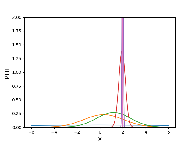
Using a normal distribution the CE procedure is the following:

• •

  Initialization : at the first iteration $k=0$, a mean $\boldsymbol{\mu}^{0}\in\mathbb{R}^{n}$ and a standard deviation $\boldsymbol{\sigma}^{0}\in\mathbb{R}^{n}$ (with $n$ the dimension of the problem) are arbitrarily chosen. A large value of $\boldsymbol{\sigma}^{0}$ is taken in order to escape from local solutions.

• •

  Iterative part: at each iteration $k\geq 1$:

  • –

    First, a sample $\textbf{X}_{1},...,\textbf{X}_{N_{s}}$ of points in $\mathbb{R}^{n}$ is generated from a normal law
    $\mathcal{V}(\boldsymbol{\mu}^{k-1},\boldsymbol{\sigma}^{k-1})$ where $N_{s}$ is the number of samples.

  • –

    Then, $f$ is evaluated at each sampled points and a number of elite points $N_{e}$, with the lowest value of f. $\boldsymbol{\mu}^{k}$ and $\boldsymbol{\sigma}^{k}$ are the mean and standard deviation of these $N_{e}$ points.

  • –

    Termination: once the standard deviation becomes sufficiently small, the procedure is stopped.

The sequence of normal distribution is illustrated in the right part of Figure 1. This example shows how the CE procedure escapes from the local minimum at $x=-2$ and converges in seven iterations to the neighborhood of $x=2$.

Before presenting the CE method introduced in CE-Ru-Kr-SP, the ASP is considered and the two iterative steps of the algorithm are precised. Problem 1 is transformed into an ASP. Using a family of probability distribution functions (pdf) $\{g(\cdot;\textbf{v}):\textbf{v}\in\mathcal{V}\}$ where $g$ is the law chosen to sample the different points at each iteration. $\mathcal{V}$ is the set of vector parameters of the pdf $g$ which are calculated at each iteration. In the previous example $g$ is taken as the normal law and the $\textbf{v}^{k}\in\mathcal{V}$ is composed of the mean and standard deviation $\textbf{v}^{k}=(\boldsymbol{\mu}^{k},\boldsymbol{\sigma}^{k})$. Having explained the law and its parameters, the ASP related to problem 1 can be defined as follows:

where $\textbf{v}\in\mathcal{V}$ is a vector of parameter, X is a random vector with a pdf $g(\cdot;\textbf{v})$ and $\gamma$ is a variable. At this stage, for a given value of $\gamma$, the parameter v may be estimated. Conversely, given a vector of parameters v, the value $\gamma$ may be also estimated. The CE method is based on these two estimations, at each iterations, the algorithm estimates one then the other. In the iterative part of Example 3, the first item corresponds to the estimation of $\gamma$ and the second one to the estimation of v. More precisely, we denote $\gamma^{*}\in\mathbb{R}$ as the infemum of the objective function, $\textbf{v}^{*}$ the parameters and $g(\cdot;\textbf{v}^{*})$ the pdf associated to this infemum. The goal is to generate a sequence $(\gamma^{k},\textbf{v}^{k})$ converging to $(\gamma^{*},\textbf{v}^{*})$. To achieve this goal, a sequence of pdf $g(\cdot;\textbf{v}^{0}),g(\cdot;\textbf{v}^{1}),...$ converging to $g(\cdot;\textbf{v}^{*})$ is created. To assure the convergence, one must have a “measure” of the difference between the iterate pdf $g(\cdot;\textbf{v}^{k})$ and the objective one $g(\cdot;\textbf{v}^{*})$. The Kullback-Leibler (KL) divergence KuLe is used:

The iterative steps may now be described. $\rho$ is defined as a very small quantity, corresponding to the proportion of elite points which are kept from an iteration to another. The procedure is:

• •

  Adaptive update of $\gamma^{k}$. With a fixed parameter of pdf $\textbf{v}^{k-1}$, $\gamma^{k}$ is defined such that it is the $(1-\rho)$-quantile of $f(\textbf{X})$ under $v_{k-1}$. Then, $\gamma^{k}$ satisfies:

  $$P_{\textbf{v}^{k-1}}(f(\textbf{X})\leq\gamma^{k})\geq\rho,$$

  (6)

  $$P_{\textbf{v}^{k-1}}(f(\textbf{X})\geq\gamma^{k})\geq 1-\rho$$

  (7)

  where $X\sim g(\cdot;\textbf{v}^{k-1})$. The $\gamma^{k}$ is denoted $\hat{\gamma}^{k}$. To obtain this estimator, a sample $\textbf{X}_{1},...,\textbf{X}_{N_{s}}$ is drawn from $g(\cdot;\textbf{v}^{k-1})$ and evaluated. Then, the $(1-\rho)$ quantile is:

  $$\hat{\gamma}^{k}=f_{\lceil(1-\rho)N_{s}\rceil}.$$

  (8)

• •

  Adaptive update of $\textbf{v}^{k}$. With a fixed $\gamma^{k}$ and knowing $\textbf{v}^{k-1}$, $\textbf{v}^{k}$ is a solution of:

  $$\begin{split}\max_{\textbf{v}}D(\textbf{v})&=\max_{\textbf{v}}E_{\textbf{v}^{k-1}}\Big(I_{\{f(\textbf{X})\leq\gamma^{k}\}}\ln(g(\textbf{X};\textbf{v}))\Big)\\ &=\min_{\textbf{v}}E_{\textbf{v}^{k-1}}\Bigg(I_{\{f(\textbf{X})\leq\gamma^{k}\}}\ln\left(\frac{I_{\{f(\textbf{X})\leq\gamma^{k}\}}}{g(\textbf{X};\textbf{v})}\right)\Bigg)\end{split}$$

  (9)

  which is the minimization of the KL divergence at iteration $k$ (with the convention $0\ln(0)=0$). Nevertheless, in practice, the real expectation and the real $\gamma^{k}$ are not known, estimators must be used and the following equation is solved:

  $$\tilde{\textbf{v}}^{k}\in\mathop{\mathrm{argmax}}_{\textbf{v}}\widehat{D}(\textbf{v})=\frac{1}{N_{s}}\sum_{i=1}^{N_{s}}I_{\{f(\textbf{X}_{i})\leq\widehat{\gamma}^{k}\}}\ln(g(\textbf{X}_{i};\textbf{v}).$$

  (10)

Last but not least, $\hat{\textbf{v}}^{k}$ is not set to $\tilde{\textbf{v}}^{k}$. There are two reasons for that: first the value of $\tilde{\textbf{v}}^{k}$ are smoothed. Second, some components of $\tilde{\textbf{v}}^{k}$ could be set to 0 or 1 at the first few iterations and the algorithm could converge to non optimal solution. To avoid these problems, the authors of CE-Ru-Kr-SP propose to use the following convex combination:

with $0<\alpha\leq 1$. Theoretically, any distribution converging in the neighborhood where the global maximum is attained can be used including normal, double exponential or beta distribution. Nevertheless, the beta distribution has for support $[0,1]$ which is not suitable for global exploration, the double exponential may introduce some discontinuities and the updating step is quite simple with the normal distribution. Thus, in practice the normal distribution is often chosen lopez2016gace miarnaeimi2018multi 6718058. Therefore, the detailed algorithm is presented next:

Section 2 presented the CE method for unconstrained optimization. In CE-Ru-Kr-SP, the bound constrained case is treated using a truncated normal law and a penalty approach is used for inequality constraints. In our work, the truncated normal law is also used to treat the bound constraints. For general inequality constraints, the algorithm does not use the penalty approach. The proposed approach is derived from the progressive barrier method described in Section 2.1. In fact, when the algorithm chooses the elite sample, it uses the following function Best (defined in G-2017-90 and recalled here). Thus, any points in the cache may be selected even if its value of constraint violation is over the threshold of progressive barrier AuDe09a. The definition relies on both the objective and the constraint violation functions $f$ and $h$.

The function Older gives the point which was generated before the former one. Thanks to this definition, CE may treat the general inequality constraints with the terminology used in Mads.

Three elements differ compared to classical CE method concerning the mean and the standard deviation. First, the elite points taken to compute the mean and the standard deviation are not only the $N_{s}$ points generated by the normal law. The elite points are chosen from the cache at the iteration $k$, denotes $V^{k}\subset\mathbb{R}^{n}$, so any points generated by the Mads algorithm may be selected. This set is ordered with the function Best, in order to select the $N_{e}$ elite points, it is sufficient to take the $N_{e}$ first points of $V^{k}$.

Second, the mean and the standard deviation initialization procedure differs from the CE method proceeds. Indeed, Mads always begins with a starting point, thus there is at least one point in the cache (the set of evaluated points). Moreover, to avoid generating trial points far from the current solution, bounds are added to the problem as follows (using $\bar{\textbf{x}}^{k}$ the poll center at iteration $k$):

where $\Delta^{\max}_{i}=\max\{\Delta^{0}_{i},...,\Delta^{k}_{i}\}$ for each $i\in[1,n]$. The sequance $(\Delta^{\max}_{i})_{k}$ is non decreasing with respect to $k$ and the product $\tau^{-1}\Delta_{i}^{\max}$ is always larger than $\Delta_{i}$ since $\tau^{-1}>1$. Once the problem has finite bound constraints, there are two cases to calculate the mean $\boldsymbol{\mu}^{k}\in\mathbb{R}^{n}$ and the standard deviation $\boldsymbol{\sigma^{k}}\in\mathbb{R}^{n}$:

• •

  In case where the number of points in the cache is too small to be relevant, i.e. fewer points that the number $N_{e}$ required, then the mean and the standard deviation are determined such that:

  	$\displaystyle\boldsymbol{\mu}^{k}$	$\displaystyle=\bar{\textbf{x}}^{k}$		(13)
  	$\displaystyle\boldsymbol{\sigma}^{k}$	$\displaystyle=2(\textbf{u}^{k}-\boldsymbol{\ell}^{k})$		(14)

• •

  In the others cases, the same calculations are made that in the original CE process:

  	$\displaystyle\boldsymbol{\mu}^{k}$	$\displaystyle=\frac{1}{N_{e}}\displaystyle\sum_{j\in E^{k}}\textbf{X}_{j}$
  	$\displaystyle[\boldsymbol{\sigma}^{k}]_{i}$	$\displaystyle=\displaystyle\sqrt{\frac{1}{N_{e}-1}\displaystyle\sum_{j\in E^{k}}[\textbf{X}_{j}-\boldsymbol{\mu}^{k}]_{i}^{2}},\;\forall i\in[1,n].$

Third, to generate the point during the CE search, the truncated normal law was always used with the bounds created in (12). Moreover, the elite points come not only from the previous normal sampling but also of the other kind of search step. That gives a vector of standard deviation which tends to zero very quickly, the other methods doing generally a local search. That is why, the standard deviation is calculated as in 11 with a coefficient $\alpha=0.7$.

The goal of the CE method is to explore in few evaluations the space to determine the promising region. The number of evaluations used by the CE search step must be quite small. For this purpose, Mads does not perform the CE search step at every iteration. The standard deviation can be seen as a measure of the incertitude on the data and is used to determine whether to launch the search step or not. First, a new variable called $\boldsymbol{\sigma}^{p}$ is introduced, it represents the incertitude measured the last time the algorithm passed through the CE search step and generated trial points. This variable is initialized to $\infty$. Then, the condition to launch the CE search is the following:

This conditions means that the current incertitude is smaller than the previous one. Each time this conditions is respected, $\boldsymbol{\sigma}^{p}$ is updated with the standard deviation obtained after the CE step. Last but not least, there is a special case. The CE method being associate with Mads which is a local search, it is possible that the points become rapidly close to each others, reducing the standard deviation. In some cases, that avoids to escape from unfeasible region. Thus, in case where several iterations of Mads algorithm are passed and the feasible region is still not reached, then the CE- SEARCH is launched with a mean equal to the current best point and a standard deviation equal to 2 times the initial standard deviation until a feasible point is found.

The Mads-default (no models), CE-Mads, VNS-Mads and LH-Mads are tested to solve a simple multidisciplinary wing design optimization problem Giun97a. Each initial point defines a MDO problem. Solving the problem consists in maximizing the range of an aircraft subject to 10 general constraints. The problem has 10 scaled design variables bounded in $[0;100]$. Figure 8 shows the result on a data profile when solving 20 MDO problems on different initial points using 3000 function evaluations or less. The initial points are real randomly selected within the bounds. Each run is done with three different seeds in order to minimize the impact of the seed.

Figure 8 shows that the CE-Mads outperforms the other algorithms for all values of $\tau$. Given that the computational time of engineering test problem is relatively low, the comparison between the heuristics and the MADS-type algorithm can be done. The inequality constraints are handled by the default setting in pymoo which is a penalization method. Given that Mads and VNS-Mads require a starting point to be run which can impact their performance, they are not used in this comparison. Therefore, we do not use any starting point but the different algorithms are run with 20 different seeds. The result are given on the figure 9. The heuristics perform poorly compared to the Mads-type algorithm. That is not surprising given that Mads benefits of a specialized method to handle the constraints and is specialized in blackbox optimization. The tests on the other engineering test problems are not presented given the great computational time required and the even harder optimization of the blackbox.

The Mads-default (no models), CE-Mads, VNS-Mads and LH-Mads algorithms are tested to optimize a styrene production process AuBeLe08, called STYRENE. This problem is a simulation of a chemical process. This process relies on a series of interdependent calculation of blocks using common numerical tools as Runge-Kutta, Newton, fixed point and also chemical related solver. The particularity of this problem is the presence of “hidden” constraints, i.e. sometimes the process does not finish and just return an error. In the case where the chemical process ends, the constraints (not hidden) and the objective functions may be evaluated during a post-processing. The objective is to maximize the net value of the styrene production process with 9 industrial and environmental regulations constraints.

In this work, a STYRENE problem possesses eight independent variables influencing the styrene production process. The variables considered during the optimization process are all scaled and bounded in $X=[0,100]^{8}$. As it was done for the MDO test problems, the four algorithms are tested with 20 different starting points taken in $\mathcal{X}$. A maximal number of evaluations of 3000 is used and each problem is run with three different seeds. The STYRENE problems is particularly interesting in this study, because there are two minima as it is shown in G-2017-90. The results with $\tau=10^{-1}$ allow to know the percentage of problems having found the global minimum. The results are provided on Figure 10. On the left plot, it is interesting to notice that the CE-Mads algorithm find the global minimum the same number of times that the LH-Mads algorithm but is more efficient. On the right plot, the CE-Mads algorithm seems to have the same accuracy that the VNS-Mads algorithm and is slightly more efficient.

Finally, the Mads default (no models), LH-Mads and CE-Mads algorithms without quadratic models are tested to solve the basic version of a pump-and-treat groundwater remediation problem from Montana Lockwood Solvent Groundwater Plume Site matott_lockwood, called LOCKWOOD. The problem has 6 design variables bounded in $X=[0,20000]^{6}$ and 4 constraints. A particularity of this problem is that each simulation run take several seconds, so the maximum number of blackbox evaluations is set to 1500. The algorithms are started from 20 different randomly selected initial points in $X$ and three different seeds are used as previously. The results are provided on Figure 11.

In this problem, reach the feasible region is not easy. Here again, the results at $\tau=10^{-1}$ allows to give an idea of the number of times the algorithm reach the feasible region. For instance, CE-Mads and LH-Mads always reach the feasible region while Mads default reaches the feasible only 41 times on 60 instances and VNS-Mads only 46 times. The efficiency of CE-Mads and LH-Mads is comparable. However, on the right plot, a better accuracy is reached with a greater efficiency by the CE-Mads algorithm.

References

- (1) Audet, C., Béchard, V., Le Digabel, S.: Nonsmooth optimization through Mesh Adaptive Direct Search and Variable Neighborhood Search. Journal of Global Optimization 41(2), 299–318 (2008). DOI 10.1007/s10898-007-9234-1. URL http://dx.doi.org/doi:10.1007/s10898-007-9234-1
- (2) Audet, C., Dennis, Jr., J.: Mesh Adaptive Direct Search Algorithms for Constrained Optimization. SIAM Journal on Optimization 17(1), 188–217 (2006). DOI 10.1137/040603371. URL http://dx.doi.org/doi:10.1137/040603371
- (3) Audet, C., Dennis, Jr., J.: A Progressive Barrier for Derivative-Free Nonlinear Programming. SIAM Journal on Optimization 20(1), 445–472 (2009). DOI 10.1137/070692662. URL http://dx.doi.org/10.1137/070692662
- (4) Audet, C., Dennis, Jr., J., Le Digabel, S.: Parallel Space Decomposition of the Mesh Adaptive Direct Search Algorithm. SIAM Journal on Optimization 19(3), 1150–1170 (2008). DOI 10.1137/070707518. URL http://dx.doi.org/10.1137/070707518
- (5) Audet, C., Hare, W.: Derivative-Free and Blackbox Optimization. Springer Series in Operations Research and Financial Engineering. Springer International Publishing, Berlin (2017). DOI 10.1007/978-3-319-68913-5. URL https://dx.doi.org/10.1007/978-3-319-68913-5
- (6) Audet, C., Kokkolaras, M., Le Digabel, S., Talgorn, B.: Order-based error for managing ensembles of surrogates in mesh adaptive direct search. Journal of Global Optimization 70(3), 645–675 (2018). DOI 10.1007/s10898-017-0574-1. URL http://rdcu.be/wGt6
- (7) Audet, C., Le Digabel, S., Tribes, C.: Dynamic scaling in the mesh adaptive direct search algorithm for blackbox optimization. Optimization and Engineering 17(2), 333–358 (2016). DOI 10.1007/s11081-015-9283-0. URL http://dx.doi.org/10.1007/s11081-015-9283-0
- (8) Audet, C., Le Digabel, S., Tribes, C.: The Mesh Adaptive Direct Search Algorithm for Granular and Discrete Variables. SIAM Journal on Optimization 29(2), 1164–1189 (2019). DOI 10.1137/18M1175872. URL https://doi.org/10.1137/18M1175872
- (9) Audet, C., Tribes, C.: Mesh-based Nelder-Mead algorithm for inequality constrained optimization. Computational Optimization and Applications 71(2), 331–352 (2018). DOI 10.1007/s10589-018-0016-0. URL https://link.springer.com/article/10.1007/s10589-018-0016-0
- (10) Blank, J., Deb, K.: Pymoo: Multi-objective optimization in python. IEEE Access 8, 89497–89509 (2020)
- (11) Booker, A., Cramer, E., Frank, P., Gablonsky, J., Dennis, Jr., J.: Movars: Multidisciplinary optimization via adaptive response surfaces. AIAA Paper 2007–1927 (2007). URL http://pdf.aiaa.org/preview/CDReadyMSDM07_1473/PV2007_1927.pdf
- (12) Chen, X., Wang, N.: Optimization of short-time gasoline blending scheduling problem with a DNA based hybrid genetic algorithm. Chemical Engineering and Processing: Process Intensification 49(10), 1076–1083 (2010). DOI 10.1016/j.cep.2010.07.014. URL http://dx.doi.org/10.1016/j.cep.2010.07.014
- (13) Clarke, F.: Optimization and Nonsmooth Analysis. John Wiley & Sons, New York (1983). URL http://www.ec-securehost.com/SIAM/CL05.html. Reissued in 1990 by SIAM Publications, Philadelphia, as Vol. 5 in the series Classics in Applied Mathematics
- (14) Conn, A., Le Digabel, S.: Use of quadratic models with mesh-adaptive direct search for constrained black box optimization. Optimization Methods and Software 28(1), 139–158 (2013). DOI 10.1080/10556788.2011.623162. URL http://dx.doi.org/10.1080/10556788.2011.623162
- (15) Conn, A., Scheinberg, K., Vicente, L.: Introduction to Derivative-Free Optimization. MOS-SIAM Series on Optimization. SIAM, Philadelphia (2009). DOI 10.1137/1.9780898718768. URL http://dx.doi.org/10.1137/1.9780898718768
- (16) Fletcher, R., Leyffer, S.: Nonlinear programming without a penalty function. Mathematical Programming Series A, 91, 239–269 (2002). DOI 10.1007/s101070100244. URL http://dx.doi.org/10.1007/s101070100244
- (17) Giunta, A.: Aircraft multidisciplinary optimization using design of experiments theory and response surface modeling methods. Ph.D. thesis, Virginia Tech, Houston, Texas (1997; available as Tech. Rep. MAD 97-05-01, May 1997, Department of Aerospace and Ocean Engineering, Virginia Tech, 215 Randolph Hall, Blacksburg, Virginia 24061)
- (18) Goldberg, D.: Genetic Algorithms in Search, Optimization and Machine Learning, 1st edn. Addison-Wesley Longman Publishing Co., Inc., Boston, MA, USA (1989)
- (19) Gould, N., Orban, D., Toint, P.: CUTEr (and SifDec): A constrained and unconstrained testing environment, revisited. ACM Transactions on Mathematical Software 29(4), 373–394 (2003). DOI 10.1145/962437.962439. URL http://dx.doi.org/10.1145/962437.962439
- (20) Hansen, N.: The CMA Evolution Strategy: A Comparing Review. In: J. Lozano, P. Larrañaga, I. Inza, E. Bengoetxea (eds.) Towards a New Evolutionary Computation, Studies in Fuzziness and Soft Computing, vol. 192, pp. 75–102. Springer Berlin Heidelberg (2006). DOI 10.1007/3-540-32494-1˙4. URL http://dx.doi.org/10.1007/3-540-32494-1_4
- (21) Hedar, A.R.: Global Optimization Test Problems. http://www-optima.amp.i.kyoto-u.ac.jp/member/student/hedar/Hedar_files/TestGO.htm. URL http://goo.gl/0vxil. (last accessed on 2017-10-20)
- (22) Hock, W., Schittkowski, K.: Test Examples for Nonlinear Programming Codes, Lecture Notes in Economics and Mathematical Systems, vol. 187. Springer, Berlin, Germany (1981)
- (23) Jahn, J.: Introduction to the Theory of Nonlinear Optimization. Springer, Berlin (1994). URL http://www.springer.com/mathematics/book/978-3-540-49378-5
- (24) Jamil, M., Yang, X.S.: A literature survey of benchmark functions for global optimisation problems. International Journal of Mathematical Modelling and Numerical Optimisation 4(2), 150–194 (2013). DOI 10.1504/IJMMNO.2013.055204. URL http://dx.doi.org/10.1504/IJMMNO.2013.055204
- (25) Kennedy, J., Eberhart, R.: Particle swarm optimization. In: Proceedings of the 1995 IEEE International Conference on Neural Networks, pp. 1942–1948. IEEE Service Center, Piscataway, Perth, Australia (1995)
- (26) Kitayama, S., Arakawa, M., Yamazaki, K.: Sequential approximate optimization using radial basis function network for engineering optimization. Optimization and Engineering 12(4), 535–557 (2011). DOI 10.1007/s11081-010-9118-y. URL http://dx.doi.org/10.1007/s11081-010-9118-y
- (27) Kroese, D.P., S.Porotsky, Rubinstein, R.Y.: The Cross-Entropy method for continuous and multi-extremal optimization. Metodol Comput Appl Probab 8, 383–407 (2006). DOI 10.1007/s11009-006-9753-0
- (28) Kullback, S., R.Leibler: On information and sufficiency. Annals of Mathematical Statistics 22, 79–86 (1951)
- (29) Le Digabel, S.: Algorithm 909: NOMAD: Nonlinear Optimization with the MADS algorithm. ACM Transactions on Mathematical Software 37(4), 44:1–44:15 (2011). DOI 10.1145/1916461.1916468. URL http://dx.doi.org/10.1145/1916461.1916468
- (30) Lopez-Garcia, P., Onieva, E., Osaba, E., Masegosa, A.D., Perallos, A.: Gace: A meta-heuristic based in the hybridization of genetic algorithms and cross entropy methods for continuous optimization. Expert Systems with Applications 55, 508–519 (2016)
- (31) Lukšan, L., Vlček, J.: Test problems for nonsmooth unconstrained and linearly constrained optimization. Tech. Rep. V-798, ICS AS CR (2000). URL http://www.cs.cas.cz/ics/reports/v798-00.ps
- (32) Matott, L., Rabideau, A., Craig, J.: Pump-and-treat optimization using analytic element method flow models. Advances in Water Resources 29(5), 760–775 (2006). DOI 10.1016/j.advwatres.2005.07.009. URL http://dx.doi.org/10.1016/j.advwatres.2005.07.009
- (33) McKinnon, K.: Convergence of the Nelder-Mead simplex method to a nonstationary point. SIAM Journal on Optimization 9(1), 148–158 (1998). DOI 10.1137/S1052623496303482. URL https://dx.doi.org/10.1137/S1052623496303482
- (34) Mezura-Montes, E., Coello, C.: Useful Infeasible Solutions in Engineering Optimization with Evolutionary Algorithms. In: Proceedings of the 4th Mexican International Conference on Advances in Artificial Intelligence, MICAI’05, pp. 652–662. Springer-Verlag, Berlin, Heidelberg (2005). DOI 10.1007/11579427˙66. URL http://dx.doi.org/10.1007/11579427_66
- (35) MiarNaeimi, F., Azizyan, G., Rashki, M.: Multi-level cross entropy optimizer (mceo): an evolutionary optimization algorithm for engineering problems. Engineering with Computers 34(4), 719–739 (2018)
- (36) Mladenović, N., Petrović, J., Kovačević-Vujčić, V., Čangalović, M.: Solving spread spectrum radar polyphase code design problem by tabu search and variable neighbourhood search. European Journal of Operational Research 151(2), 389–399 (2003). DOI 10.1016/S0377-2217(02)00833-0. URL http://dx.doi.org/10.1016/S0377-2217(02)00833-0
- (37) Moré, J., Garbow, B., Hillstrom, K.E.: Testing unconstrained optimization software. ACM Transactions on Mathematical Software 7(1), 17–41 (1981). DOI 10.1145/355934.355936. URL http://dx.doi.org/10.1145/355934.355936
- (38) Moré, J., Wild, S.: Benchmarking derivative-free optimization algorithms. SIAM Journal on Optimization 20(1), 172–191 (2009). DOI 10.1137/080724083. URL http://dx.doi.org/10.1137/080724083
- (39) Pigache, F., Messine, F., Nogarede, B.: Optimal Design of Piezoelectric Transformers: A Rational Approach Based on an Analytical Model and a Deterministic Global Optimization. IEEE Transactions on Ultrasonics, Ferroelectrics, and Frequency Control 54(7), 1293–1302 (2007). DOI 10.1109/TUFFC.2007.390. URL http://dx.doi.org/10.1109/TUFFC.2007.390
- (40) Price, K., Storn, R.M., Lampinen, J.A.: Differential evolution: a practical approach to global optimization. Springer Science & Business Media (2006)
- (41) R. Storne, K.P.: Differential Evolution - A simple and efficient heuristic for global optimization over continuous spaces. Journal of Global optimization 11, 341–359 (1997)
- (42) Rodríguez, J., Renaud, J., Watson, L.: Trust Region Augmented Lagrangian Methods for Sequential Response Surface Approximation and Optimization. Journal of Mechanical Design 120(1), 58–66 (1998). DOI 10.1115/1.2826677. URL http://dx.doi.org/10.1115/1.2826677
- (43) Rubinstein, R.Y.: Optimization of computer simulation models with rare events . European Journal of Operational Research 99, 89–112 (1997)
- (44) Rubinstein, R.Y., Kroese, D.P.: The Cross-Entropy Method: A unified Approach to Combinatorial Optimization, Monte-Carlo Simulation and Machine Learning. Springer: Berlin Heidelberg, New York, USA (2004)
- (45) Stein, M.: Large sample properties of simulations using latin hypercube sampling. Technometrics 29(2), 143–151 (1987). URL http://www.jstor.org/stable/1269769
- (46) Subathra, M.S.P., Selvan, S.E., Victoire, T.A.A., Christinal, A.H., Amato, U.: A hybrid with cross-entropy method and sequential quadratic programming to solve economic load dispatch problem. IEEE Systems Journal 9(3), 1031–1044 (2015). DOI 10.1109/JSYST.2013.2297471
- (47) Tao, J., Wang, N.: DNA Double Helix Based Hybrid GA for the Gasoline Blending Recipe Optimization Problem. Chemical Engineering and Technology 31(3), 440–451 (2008). DOI 10.1002/ceat.200700322. URL http://dx.doi.org/10.1002/ceat.200700322
- (48) Wang, K., Wang, N.: A novel RNA genetic algorithm for parameter estimation of dynamic systems. Chemical Engineering Research and Design 88(11), 1485–1493 (2010). DOI 10.1016/j.cherd.2010.03.005. URL https://doi.org/10.1016/j.cherd.2010.03.005