Bayesian nonparametric panel Markov-switching GARCH models??
Abstract
This paper introduces a new model for panel data with Markov-switching GARCH effects. The model incorporates a series-specific hidden Markov chain process that drives the GARCH parameters. To cope with the high-dimensionality of the parameter space, the paper exploits the cross-sectional clustering of the series by first assuming a soft parameter pooling through a hierarchical prior distribution with two-step procedure, and then introducing clustering effects in the parameter space through a nonparametric prior distribution. The model and the proposed inference are evaluated through a simulation experiment. The results suggest that the inference is able to recover the true value of the parameters and the number of groups in each regime. An empirical application to 78 assets of the SP&100 index from January 2000 to October 2020 is also carried out by using a two-regime Markov switching GARCH model. The findings shows the presence of 2 and 3 clusters among the constituents in the first and second regime, respectively.
, and
University Ca’ Foscari of Venice?? and University of L’Aquila ??
1 Introduction
Over the last ten years, there has been an increasing interest in the study of volatility of large panels of asset returns, with a special focus on dynamic dependence and heterogeneity across assets (Pakel, Shephard and Sheppard 2011; Barigozzi, Brownlees and Veredas 2014; Ardia et al. 2018; Bollerslev, Patton and Quaedvlieg 2020). The empirical evidence has also shown the presence of regimes in the volatility of financial returns (see Ardia 2008; Ang and Timmermann 2012; Bauwens and Otranto 2016; Haas and Liu 2018, among others) and Markov switching (MS) GARCH models have been used to cope with regime changes and temporal clustering of the conditional volatility.
Several GARCH models have been proposed to account for dependence (Virbickaite, Ausín and Galeano 2015; Bauwens and Otranto 2016; Bauwens and Otranto 2020, for a review, see), but the estimation of a large number of parameters with the available data dimension remains an open issue. In this respect, evidence of cluster-wise dependence in the distribution of financial asset returns (Bauwens and Rombouts 2007, see) has prompted researcher to adopt cross-sectional clustering of the time series as a building block for a dimensionality reduction step in large dimensional problems of the parameter space (Hirano 2002; Billio, Casarin and Rossini 2019, see, for example,).
In this paper, we propose to model the cross-sectional clustering effects with a Bayesian nonparametric technique (Ferguson 1973; Lo 1984) where a hierarchical Pitman-Yor process prior (Pitman and Yor 1997) for the MS-GARCH parameters is considered. Non-parametric Bayesian techniques have been largely and successfully used in different fields such as biostatistics (Do, Muller and Tang 2005), biology Arbel, Mengersen and Rousseau 2016, medicine (Xu et al. 2016), and neuroimaging (Zhang et al. 2016). For an introduction to Bayesian non-parametrics see Hjort et al. 2010 and for a review of models and applications in different fields see Müller and Mitra 2013.
In our panel model, the first stage of the hierarchical prior allows for cross-unit heterogeneity, while shrinking all unit-specific parameters towards a common mean. The second stage of the hierarchy allows for mixed effects in the common mean. There are many advantages in using this hierarchical nonparametric prior. First, our approach allows for making inference on the number of mixture components in the cross-sectional clustering. Second, it adds flexibility to the model allowing for different shapes of the prior and posterior predictive distributions. Third, the predictive distribution incorporates uncertainty in the parameters and in the number of mixture components. Lastly, the Bayesian nonparametric combined with a data-augmentation strategy makes the inference more tractable for our high dimensional model.
The model and inference proposed in this paper are novel in some respects. As such, the paper contributes to the literature on Bayesian semiparametrics and nonparametrics for time series analysis (Taddy and Kottas 2009; Jensen and Maheu 2010; Griffin and Steel 2011; Di Lucca et al. 2013; Bassetti, Casarin and Leisen 2014; Casarin, Molina and ter Horst 2019; Billio, Casarin and Rossini 2019; Nieto‐Barajas and Quintana 2016; Griffin and Kalli 2018, e.g., see). The paper also innovates the Bayesian nonparametric dynamic panel model in Hirano 2002 by introducing Markov-switching and GARCH dynamics.
The paper also extends the nonparametric switching regression in Taddy and Kottas 2009 to a panel model with GARCH dynamics. Our approach differs from those in Hirano 2002 and Taddy and Kottas 2009, and is in line with the strategies for large dimensional and over-parametrized models (MacLehose and Dunson 2010; Wang 2010; Billio, Casarin and Rossini 2019, e.g., see), where a multiple-stage hierarchical prior is used to combine partial pooling and clustering effects in the parameter space. Further, differently from Hirano 2002 and Taddy and Kottas 2009, the paper uses a MCMC algorithm for posterior approximation that relies on the efficient sampling method developed in Walker 2007; Kalli, Griffin and Walker 2011; Hatjispyros, Nicoleris and Walker 2011. Lastly, the paper makes a contribution to the literature on Bayesian Markov-switching panel models (Kaufmann 2010; Kaufmann 2015; Billio et al. 2016; Casarin et al. 2019, e.g., see) by introducing GARCH effects and allowing for a flexible nonparametric specification.
The estimation of MS-GARCH models is also a difficult task given the path dependence problem (Gray 1996) and approximation methods have been considered (Bauwens, Preminger and Rombouts 2010; Henneke et al. 2011; Ardia 2008; Haas, Mittnik and Paolella 2004; He and Maheu 2010; Bauwens, Dufays and Rombouts 2014; Elliott et al. 2012; Dufays 2015; Wee, Chen and Dunsmuir 2020, e.g., see). In this paper, we extend the univariate Gibbs sampler by Billio, Casarin and Osuntuyi 2016 to a multiple time series set-up and provide an efficient MCMC procedure for the hidden states of a panel MS-GARCH model. The proposed method relies on a combination of Gibbs and Metropolis samplers. The model and the proposed inference are evaluated through simulation experiments. The results show that the inference is able to recover the true value of the parameters and the number of groups in each regime.
Our model is applied to 78 assets of the SP&100 index from January 2000 to October 2020. The analysis can be useful for portfolio making and style investing decisions. In particular, the analysis aims to identify the under- and over-performance regimes in expected returns. Then, clusters of assets within each regime are identified. Lastly, we use the sector classification and some fundamental financial ratios to study the composition of the clusters. The main empirical results are as follows. We find evidence of different clustering structure across regimes. Regime 1 (over-performance phase) and regime 2 (under-performance phase) comprise 2 and 3 clusters, respectively. While the composition of clusters varies across regimes, some common features are observed. In both regimes, medium size companies represent the largest majority and assets in cluster 2 seem to be overvalued by their Price-to-Earning ratio.
The paper is organized as follows. Section 2 introduces our MS-GARCH panel model and the Bayesian nonparametric prior distribution. Section 3 presents the data augmentation strategy and the posterior approximation method. In Section 4, we present a simulation study and an empirical application to the financial returns data. Section 5 concludes.
2 A Bayesian nonparametric MS-GARCH model
We assume that the observable variable for the -th unit of the panel at time satisfies
| (1) |
for and , where denotes the Gaussian distribution with location and scale . The conditional variance is as follows:
| (2) |
which is the MS-GARCH model, and , is a hidden Markov chain process with transition probability
| (3) |
where with the number of states. The following functional form for the switching parameters is specified as follows:
| (4) | |||
| (5) |
We cope with the high-dimensionality of the parameter space due to the large cross-section dimension , and related overfitting issues of the model, by exploiting cross-sectional clustering of the series. More specifically we propose to combine two modelling strategies. First, we assume soft parameter pooling through a hierarchical prior distribution with two stages, and second we introduce clustering effects in the parameter space through a nonparametric prior. The resulting joint prior distribution for the MS-GARCH parameters is given by the following.
In the first stage, the rows of the transition matrix are assumed to follow a Dirichlet distribution:
| (6) |
for all units and regimes , where the precision parameter shrinks the unit-specific probabilities toward a common value . For the second stage we assume
| (7) |
with .
To cope with the high dimension of the parameter space, in the first stage of the hierarchical prior, we shrink the switching parameters toward some common values, and in the second stage we introduce a regime-specific process which is clustering the units in groups such that for and . In the first stage, we assume the following
| (8) | |||
| (9) |
for where denotes the beta distribution with mean and is a real positive constant. The scale hyper-parameters and are shrinking toward the parameter which is assumed to be constant for all units in the same cluster, that is for all where (for further details see Section 3 and Eq. 27). Since the parameters are non-identified due to the label switching problem, we follow a commonly used approach and impose a prior restriction on the intercepts (Celeux 1998; Frühwirth-Schnatter 2001; Frühwirth-Schnatter 2006, e.g., see).
The second stage of the hierarchy is generating the clusters of parameters. For each regime we assume a Pitman-Yor process (PYP) prior
| (10) |
with base measure and concentration and dispersion parameters and , respectively. We assume is the product measure of the following independent normal and uniform distributions
| (11) |
which are usually chosen as prior distributions in parametric Bayesian inference for MS-GARCH (Billio, Casarin and Osuntuyi 2016, e.g., see). The PYP introduced in Pitman and Yor 1997 is a generalization of the Dirichlet process (DP) defined in Ferguson 1973 which can be obtained for .
Through the illustration of the Chinese Restaurant metaphor, the clustering structure of the PYP is defined by a Polya-Urn sampling scheme. The parameter of the -th unit is either equal to one of the other units or a new one from the base distribution , i.e.:
| (12) |
This sequential allocation procedure is generating clusters in the parameter space, where the number of clusters is random. The Pitman-Yor process induces the following prior distribution on the number of clusters
with , where is a generalized Stirling number of the first kind, and is the one-parameter gamma function (e.g., see Pitman 2006, Ch. 1 and 3). The following formula is used to evaluate the prior mean of the number of clusters:
We summarize our Bayesian nonparametric model in the Directed Acyclic Graph representation of Fig. 1.
It is possible to show that the PYP clustering effects on the cross section of time series correspond to a probabilistic clustering of the parameters based on an infinite mixture distribution. The Pitman-Yor process prior can be written in a Sethuraman’s like representation as a discrete random measure
| (13) |
where the atoms are i.i.d. random variables from the base measure and the random weights have the stick-breaking representation
| (14) |
with i.i.d. (Arbel, Blasi and Prünster 2019, see).
By integrating out the discrete part of the hierarchical prior one obtains the following infinite mixture representation of the prior distribution on
| (15) |
where is the joint parameter distribution at the first stage of hierarchical prior (see Eqs. 8-9) and is the distribution at the second stage. In conclusion the PYP prior allows for probabilistic clustering in the parameter space.
The predictive density induced by our prior assumptions can be written as
| (16) |
where is the transition kernel of the MS-GARCH with for and , and . This prior predictive densities accounts for various forms of possible heterogeneity in the data such as asymmetry, excess of kurtosis and multimodality.
3 Posterior approximation
Let be the collection of the unit- and regime-specific parameters and , and the collection of transition probabilities. Let be the collection over time of the observation vector and be the collection over time of the latent vectors . The likelihood function of the proposed MS-GARCH panel model is
| (17) |
where
| (18) |
which is not tractable since it is written in integral form as usually in latent variable models. Nevertheless a data-augmentation principle can be applied (Tanner and Wong 1987) in order to develop efficient posterior simulation methods. Following a common strategy in panel Markov-switching literature (Billio et al. 2016; Casarin et al. 2019; Bianchi et al. 2019, e.g., see), we introduce the set of auxiliary allocation variables which allow us to write the complete-data likelihood function as follows
| (19) |
where is the collection over time of the latent vectors with .
The joint hierarchical prior distribution is
| (20) |
where
| (21) |
is the infinite mixture prior where we recall is the first-stage joint prior distribution given in Eqs. 8-9 and
| (22) | |||||
| (23) |
is joint distribution of the infinite collection of stick-breaking variables and atoms, and , respectively, which are involved in the definition of the random measures .
The joint prior distribution in a Bayesian nonparametric framework is usually not tractable since its support is the space of the discrete random measures which are infinite-dimensional objects (see Eqs. 21-23). Nevertheless, the data-augmentation principle can be applied in order to make the inference problem more tractable. Following the recent Bayesian nonparametrics literature (Bassetti, Casarin and Leisen 2014; Bassetti, Casarin and Ravazzolo 2018; Billio, Casarin and Rossini 2019, e.g., see), we introduce a set of slice variables and define the index set . Then the infinite mixture can be demarginalized as follows
| (24) | |||||
which is a almost-surely finite mixture since a.s., where is the collection of slice variables.
Following the standard practice in finite mixture modelling we introduce the latent allocation variable and obtain
| (25) |
where . Let us denote with , and the collections of regime-specific auxiliary variables and atoms. The joint posterior distribution is proportional to
| (26) |
Note that the allocation variables allows to reconcile the notations used in the hierarchical model of Eqs. 8-11 and the random measure representation in Eqs. 13-15 as follows:
| (27) |
A Gibbs sampler is used to generate random samples from the joint posterior and to approximate the Bayesian estimator. The Gibbs sampler iterates the following steps
- 1.
Sample slice and stick-breaking variables and given
- 2.
Sample the transition probabilities given
- 3.
Sample the atoms given
- 4.
Sample the MS-GARCH parameters given
- 5.
Sample the switching allocation variables given
- 6.
Sample the mixture allocation variables given
The derivation of the full conditional distributions is given in Appendix A.
4 Numerical illustrations
4.1 Simulation results
For inference and model validation, we run a set of simulation experiments on synthetic datasets. In this section we report the results for one of the experiments, in which we examine the efficiency and effectiveness of our MCMC sampling scheme in estimating the number of clusters in each regime.
We generate a panel of 30 time series with length 300 each from the data generating process (DGP) corresponding to the model defined by Eqs. 1-9 for two regimes (), including their time-invariant transition probabilities and switching conditional mean and variance. The DGP is assumed to be as realistic as possible for illustrative purposes. In particular, the number of groups in the clusters across the two regimes is being kept relatively small.
In the first regime (i.e., ), we assume that the units are clustered into two groups with equal probability. In formulas:
In the second regime (i.e, ), the units are clustered into three groups. In formulas:
where , , and .
The transition probabilities are and i.i.d. for , where .
 |
 |
 |
 |
In Fig. 2, the true and the estimated values of the intercept () of the measurement equation and GARCH parameter (see Eqs. 1 and 2) in regime 1 (red) and 2 (blue) are illustrated.11 1 For other parameters and the trajectory of the Markov chain see Appendix 8. The findings seems to reveal that the inference is able to recover the true value of the parameters.
Figure 3 shows that data are informative about the number of clusters in each regimes, and there is a substantial revision of the prior distributions (red) and the posterior distributions (blue) concentrate about the true number of clusters in the two regimes. For our simulated dataset, the Maximum a Posteriori (MAP) estimation of the number of cluster is 1 for the first regime and 3 for the second regime.
4.2 Volatility clusters in the S&P 100
We consider 78 assets of the 101 constituents of the SP&100 index and collect the percentage log-returns at a weekly frequency. We do this to have a balanced panel of observations from January to October 2020 (the sectorial classification of these assets is reported in Tab. 1 of Appendix C).
 |
 |
 |
 |
The empirical analysis aims to identify regimes of under-performance and over-performance of expected returns. Moreover, we use the sector classification and some fundamental financial ratios to study the composition of the clusters.
As a preliminary analysis, we plot in Fig. 4 the estimates of the log-volatility and log-kurtosis of the 78 constituents considered in the analysis. This figure also shows the cross-sectional distribution of the log-volatility and log-kurtosis. The figure indicates that volatility and kurtosis change over time with time series clustering effects (see top plots of Fig. 4). This seems to suggests the use of GARCH and Markov-switching models. Furthermore, the cross-sectional distribution of the volatility and kurtosis exhibits multiple modes and long tails (see bottom plots of Fig. 4).22 2 In Fig. 11 of Appendix C, we also report the estimates of the cross-sectional distribution of the log-volatility (left) and log-kurtosis (right) of the SP&100’s constituents log-returns in the three dates ( July 2002, August 2008 and February 2020) for three different sizes of the rolling window. The results show that the preliminary evidence on cross-sectional heterogeneity is robust with respect to the choice of the window size. This fact seems to imply cross-section heterogeneity in the data with possible clustering effects in the parameters of the GARCH process. These effects cannot be captured only by a Markov-switching (MS) model, therefore there is a need of combining the MS-GARCH with a probabilistic clustering mechanism.
|
|
 |
 |
 | |
In our analysis, we first identify the two regimes, and then the clusters of assets within each regime. Lastly, we use the sector classification and some fundamental financial ratios to study the composition of the clusters.
Regime identification is achieved by ordering the expected returns , such that regime 1 corresponds to a relative over-performance state and regime 2 to an under-performance one. This identification constraint is strongly supported by the data and allows us to separate the assets returns in two performance regimes (see Fig. 12 in Appendix C).
Regarding the cluster identification, Fig. 5 reports the prior (red) and posterior (blue) distribution of the number of clusters in regime 1 (left) and 2 (right). We set and in the PYP prior in order to have quite diffuse prior distributions. The posterior distribution is concentrated suggesting a substantial revision of the prior information and the MAP estimates of the number of clusters is 2 and 3 for regime 1 and 2, respectively.
 |
 |
 |
 |
 |
 |
We also estimate the co-clustering probability matrix to delve into the composition of the clusters. In this way, the probability that the parameters and are in the same cluster is given. This probability can be easily approximate by using the MCMC samples as follow
| (28) |
where is a sample of the allocation variable for the -unit parameters in the regimes and contains the values of MCMC iterations such that the parameters of the panel units have been allocated to exactly mixture components. Note that a spectral clustering algorithm have been applied to re-order the series and to provide better graphical representation of the clusters.
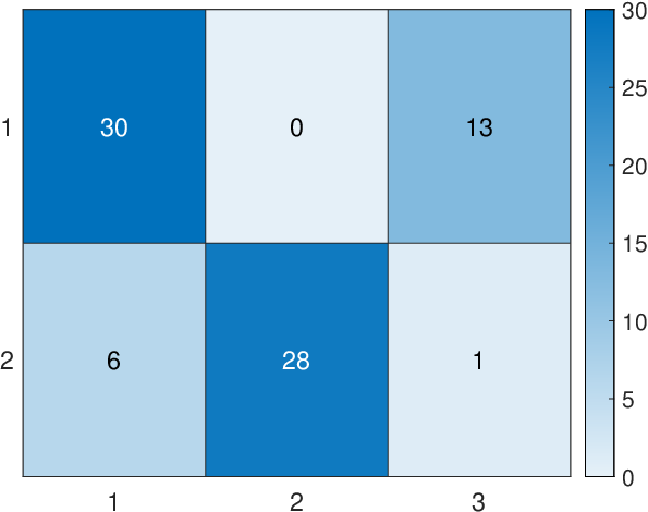
The top panel of Fig. 6 report the co-clustering matrices for the two regimes. In each block matrix, the algorithm identifies a constituent (asset) belonging to a cluster with the label 1 (color patch) and 0 (white patch) otherwise. The colors represent the sectors in the clusters. Following Wade and Ghahramani 2018, we use the variation of information (VI) metric proposed by Meilâ 2007 to compare the two regimes (in terms of clusters). This measure compares the information in the two regimes with the information shared between the two regimes. We compute the normalized value of VI (0.20), which suggests a substantial difference between the clustering and composition in the two regimes.33 3 VI lies in the interval and a normalize value is obtained dividing VI by .
The bottom panel of Fig. 6 shows the relationship between the clustering structures of the two regimes. We order the clusters following the numbers of constituents from the largest to the smallest. Most of the assets in cluster 1 in the first regime belong to cluster 1 in the second regime, whereas many assets of the first group in regime 1 belong to the third group in regime 2. In particular, for cluster 1 in both regimes, we observe that the majority of the sectors representing the assets are: manufacturing (about 40% in both regimes), financial and insurance (19% in the first regime), and wholesale and retail (25% in the second regime). Similar results for the sectors are found for cluster 2 in the two regimes. More specifically, the manufacturing sector represents about 40% of the assets in the two regimes, while the financial and insurance sector is about 18% for regime 2, and information and communication is around 20% (for details on sectors see Tabs. 2 and 3 in Appendix C).
Further, in order to characterize the clusters in terms of the market size of the constituents, we first rank the companies by computing the average size of each of them using the last year of the sample period. Then, we classify the assets into three groups, namely small (bottom 30%), medium (middle 40%) and big (top 30%) companies (see Tab. 4). We also compute the percentage of companies belonging to the clusters in each regime in terms of size. In regime 1, companies with the medium size represent the largest majority about 40%, and a similar outcome is also observed for regime 2. More specifically, the following emerge.
In regime 1, we have:
- 1.
Cluster 1 is characterized by 40% and 20% small and large size companies, respectively. This cluster also shows values on average of the market size, returns and their standard deviation equal to and , respectively. 44 4 We computed the average return and standard deviation using the whole sample, while the average market size is calculated using the last 10 years of the sample period.
- 2.
Cluster 2 consists of 17% small and 42% medium size companies with an average market size of , a return equal to and standard deviation of .
The clusters composition in Regime 2 is as follows:
- 1.
Cluster 1 comprises of small (39%) and medium size firms (36%) with an average market size of , return of and standard deviation of .
- 2.
17% and 42% of the assets in cluster 2 are small and medium size companies, respectively. While, on average the market capitalization, return and standard deviation are and , respectively.
- 3.
Cluster 3 is characterized by 29% small and 50% medium size companies. Moreover, the average market capitalization, returns and standard deviation are and .
For the cluster composition, we also compute the value of the Price-to-Earnings ratio (PE) for all the clusters55 5 Following the standard practice in style analysis the average PE is computed over the last 10 years.. For regime 1, clusters 1 and 2 have values of PE equal to 26.97 and 32.38, respectively. For regime 2, these values are 27.08, 35.69 and 23.72 for clusters 1, 2 and 3, respectively. These results seem to indicate that in both regimes cluster 2 is overvalued.
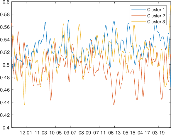
To provide additional information on the composition of the clusters, we plot the dynamics over time of the average probabilities of the assets in each cluster, the market size and the PE in Fig. 7. Regarding the average probabilities, cluster 1 shows the highest probability in regime 1, while in regime 2 clusters 1 and 3 display similar probabilities. As for PE, the dynamics in clusters 1 and 2 in regime 1 resemble those in regime 2 (see second line of Fig. 7), and the market capitalization pattern indicates that relatively to cluster 1 in the over-performance state, assets in cluster 2 seems to show lowest values before the 2008/09 Global financial crisis and larger afterwards. The same dynamics for this two clusters is also observed in the under-performance state.
The following summarizes the results. There is evidence of time-varying clustering structures in our panel of time series. Regime 1 (over-performance phase) and regime 2 (under-performance phase) comprise 2 and 3 clusters, respectively. The composition of the clusters varies across regimes while some similarities in terms capitalization and financial ratios are observed. In regime 1 and 2 medium size companies represent the largest majority (about 40%) and assets in cluster 2 seem to be over valued by their PE ratio. The pattern of the market capitalization is similar across the two regimes as cluster 2 shows lower (larger) values compared to cluster 1 before (after) the 2008/09 Global financial crisis.
5 Conclusion
The increase of interest in the study of volatility of large panels of asset returns and the evidence of regimes in volatility of financial returns has suggested to adapt Markov switching models to GARCH effect. In this respect, this paper introduces a new model for panel data with Markov-switching GARCH effects.
In particular, we propose to model cross-sectional clustering effects with a Bayesian nonparametric technique that considers a hierarchical Pitman-Yor process prior for the Markov Switching GARCH parameters. The Bayesian nonparametric approach is a two-stage procedure. In the first stage, the hierarchical prior allows for cross-unit heterogeneity, while shrinking all unit-specific parameters towards a common mean. In the second stage, the hierarchical procedure allows for mixed effects in the common mean.
This paper makes a contribution in some respects. First, the new model allows us to make inference on the number of mixture components in the cross-sectional clustering. Second, the model is sufficiently flexible to embody different shapes of the prior and posterior predictive distributions. Third, uncertainty and the number of mixture components are incorporated in the predictive distribution. Lastly, through a data-augmentation strategy, this paper makes the inference more tractable for our high dimensional model. A simulation exercise is carried out for inference and model validation.
We apply the new model to 78 assets of the SP&100 index from January 2000 to October 2020. Our results may have some implications for portfolio making and for style investing decisions. The evidence shows that regime 1 (over-performance phase) and regime 2 (under-performance phase) differ in terms of clustering structures comprising 2 and 3 clusters, respectively. Within each regime the clusters differ substantially in terms of over-performance probability and in terms of style features, when considering capitalization and Price-to-Earnings. The heterogeneity of the clusters in terms of sectors and styles allows for portfolio diversification. Across regimes, the composition of the clusters changes, nevertheless some clusters share some similarities in terms of style features, allowing for the implementation of rotating style strategies.
Further research may consider the choice of the number of performance regimes, the sensitivity with respect to nonparametric prior specification and some forecasting comparisons with exogenous clustering models.
Acknowledgements
This research used the SCSCF multiprocessor cluster system provided by the Venice Centre for Risk Analytics (VERA) at University Ca’ Foscari of Venice.
References
- Ang and Timmermann (2012) [author] Ang, A.A. and Timmermann, A.A. (2012). Regime Changes and Financial Markets. Annual Review of Financial Economics 4 313-337.
- Arbel, Blasi and Prünster (2019) [author] Arbel, JulyanJ., Blasi, Pierpaolo DeP. D. and Prünster, IgorI. (2019). Stochastic Approximations to the Pitman–Yor Process. Bayesian Analysis 14 1201–1219. 10.1214/18-ba1127
- Arbel, Mengersen and Rousseau (2016) [author] Arbel, JulyanJ., Mengersen, KerrieK. and Rousseau, JudithJ. (2016). Bayesian nonparametric dependent model for partially replicated data: The influence of fuel spills on species diversity. The Annals of Applied Statistics 10 1496–1516. 10.1214/16-aoas944
- Ardia (2008) [author] Ardia, D.D. (2008). Financial Risk Management with Bayesian Estimation of GARCH Models: Theory and Applications, volume 612 of Lecture Notes in Economics and Mathematical Systems. Springer-Verlag, Berlin, Germany.
- Ardia et al. (2018) [author] Ardia, D.D., Bluteau, K.K., Boudt, K.K. and Catania, L.L. (2018). Forecasting Risk with Markov-switching GARCH models: A large-scale performance study. International Journal of Forecasting 34 733-747.
- Barigozzi, Brownlees and Veredas (2014) [author] Barigozzi, M.M., Brownlees, G. M.G. M. C. Gallo and Veredas, D.D. (2014). Disentangling Systematic and Idiosyncratic Dynamics in Panels of Volatility Measures. Journal of Econometrics 162 364-384.
- Bassetti, Casarin and Leisen (2014) [author] Bassetti, F.F., Casarin, R.R. and Leisen, F.F. (2014). Beta-product Dependent Pitman-Yor Processes for Bayesian Inference. Journal of Econometrics 180 49-72.
- Bassetti, Casarin and Ravazzolo (2018) [author] Bassetti, F.F., Casarin, R.R. and Ravazzolo, F.F. (2018). Bayesian Nonparametric Calibration and Combination of Predictive Distributions. Journal of the American Statistical Association 522 675-685.
- Bauwens, Dufays and Rombouts (2014) [author] Bauwens, L.L., Dufays, A.A. and Rombouts, J.J. (2014). Marginal Likelihood for Markov-switching and Change-Point GARCH. Journal of Econometrics 178 508-522.
- Bauwens and Otranto (2016) [author] Bauwens, L.L. and Otranto, E.E. (2016). Modeling the Dependence of Conditional Correlations on Market Volatility. Journal of Business and Economic Statistics 34 254-268.
- Bauwens and Otranto (2020) [author] Bauwens, L.L. and Otranto, E.E. (2020). Nonlinearities and Regimes in Conditional Correlations with Different Dynamics. Journal of Econometrics 217 496-522.
- Bauwens, Preminger and Rombouts (2010) [author] Bauwens, L.L., Preminger, A.A. and Rombouts, J.J. (2010). Theory and Inference for a Markov Switching GARCH Model. Econometrics Journal 13 218-244.
- Bauwens and Rombouts (2007) [author] Bauwens, L.L. and Rombouts, J.J. (2007). Bayesian Clustering of Many GARCH Models. Econometric Reviews 26 26 365-86.
- Bianchi et al. (2019) [author] Bianchi, D.D., Billio, M.M., Casarin, R.R. and Guidolin, M.M. (2019). Modeling Systemic Risk with Markov Switching Graphical SUR Models. Journal of Econometrics 210 58-74.
- Billio, Casarin and Osuntuyi (2016) [author] Billio, M.M., Casarin, R.R. and Osuntuyi, A.A. (2016). Efficient Gibbs Sampling for Markov Switching GARCH Models. Computational Statistics and Data Analysis 100 37-57.
- Billio, Casarin and Rossini (2019) [author] Billio, M.M., Casarin, R.R. and Rossini, L.L. (2019). Bayesian Nonparametric Sparse VAR Models. Journal of Econometrics 212 97-115.
- Billio et al. (2016) [author] Billio, M.M., Casarin, R.R., Ravazzolo, F.F. and Van Dijk, H.H. (2016). Interactions between Eurozone and US Booms and Busts: A Bayesian panel Markov-switching VAR model. Journal of Applied Econometrics 31 1352–1370.
- Bollerslev, Patton and Quaedvlieg (2020) [author] Bollerslev, T.T., Patton, A. J.A. J. and Quaedvlieg, R.R. (2020). Multivariate Leverage Effects and Realized Semicovariance GARCH Models. Journal of Econometrics 217 411-430.
- Casarin, Molina and ter Horst (2019) [author] Casarin, RobertoR., Molina, GermanG. and ter Horst, EnriqueE. (2019). A Bayesian time varying approach to risk neutral density estimation. Journal of the Royal Statistical Society: Series A (Statistics in Society) 182 165-195.
- Casarin et al. (2019) [author] Casarin, R.R., Foroni, C.C., Marcellino, M.M. and Ravazzolo, F.F. (2019). Uncertainty Through the Lenses of a Mixed-Frequency Bayesian Panel Markov Switching Model. Annals of Applied Statistics 12 2559–2586.
- Celeux (1998) [author] Celeux, GillesG. (1998). Bayesian Inference for Mixture: The Label Switching Problem. In Compstat (R.R. Payne and P.P. Green, eds.) Physica, Heidelberg.
- Di Lucca et al. (2013) [author] Di Lucca, MAM., Guglielmi, AlessandraA., Muller, PeterP. and Quintana, FAF. (2013). A Simple Class of Bayesian Nonparametric Autoregression Models. Bayesian Analysis 8 63–88.
- Do, Muller and Tang (2005) [author] Do, Kim-AnhK.-A., Muller, PeterP. and Tang, FengF. (2005). A Bayesian mixture model for differential gene expression. Journal of the Royal Statistical Society: Series C (Applied Statistics) 54 627–644. 10.1111/j.1467-9876.2005.05593.x
- Dufays (2015) [author] Dufays, ArnaudA. (2015). Infinite-State Markov-Switching for Dynamic Volatility. Journal of Financial Econometrics 14 418-460.
- Elliott et al. (2012) [author] Elliott, R. J.R. J., Lau, J. W.J. W., Miao, H.H. and Siu, T. K.T. K. (2012). Viterbi-Based Estimation for Markov Switching GARCH Models. Applied Mathematical Finance 19 1-13.
- Ferguson (1973) [author] Ferguson, T. S.T. S. (1973). A Bayesian Analysis of some Nonparametric Problems. The Annals of Statistics 1 209-230.
- Frühwirth-Schnatter (2001) [author] Frühwirth-Schnatter, SylviaS. (2001). Markov chain Monte Carlo estimation of classical and dynamic switching and mixture models. Journal of the American Statistical Association 96 194–209.
- Frühwirth-Schnatter (2006) [author] Frühwirth-Schnatter, SylviaS. (2006). Finite Mixture and Markov Switching Models. Springer, New York.
- Gray (1996) [author] Gray, S. F.S. F. (1996). Modeling the Conditional Distribution of Interest Rates as a Regime-switching Process. Journal of Financial Economics 42 27-62.
- Griffin and Kalli (2018) [author] Griffin, J.J. and Kalli, M.M. (2018). Bayesian Nonparametric Vector Autoregressive Models. Journal of Econometrics 203 267-282.
- Griffin and Steel (2011) [author] Griffin, J. E.J. E. and Steel, M. F. J.M. F. J. (2011). Stick-breaking Autoregressive Processes. Journal of Econometrics 162 383-396.
- Haas and Liu (2018) [author] Haas, M.M. and Liu, J. C.J. C. (2018). A Multivariate Regime-switching GARCH Model with an Application to Global Stock Market and Real Estate Equity Returns. Studies in Nonlinear Dynamics and Econometrics 22.
- Haas, Mittnik and Paolella (2004) [author] Haas, M.M., Mittnik, S.S. and Paolella, M.M. (2004). A new Approach to Markov Switching GARCH Models. Journal of Financial Econometrics 2 493-530.
- Hatjispyros, Nicoleris and Walker (2011) [author] Hatjispyros, S. J.S. J., Nicoleris, T. N.T. N. and Walker, S. G.S. G. (2011). Dependent Mixtures of Dirichlet Processes. Computational Statistics & Data Analysis 55 2011-2025.
- He and Maheu (2010) [author] He, Z.Z. and Maheu, J. M.J. M. (2010). Real Time Detection of Structural Breaks in GARCH Models. Computational Statistics and Data Analysis 54 2628-2640.
- Henneke et al. (2011) [author] Henneke, J. S.J. S., Rachev, S. T.S. T., Fabozzi, F. J.F. J. and Metodi, N.N. (2011). MCMC-based Estimation of Markov Switching ARMA-GARCH Models. Applied Economics 43 259-271.
- Hirano (2002) [author] Hirano, K.K. (2002). Semiparametric Bayesian Inference in Autoregressive Panel Data Models. Econometrica 70 781-799.
- Hjort et al. (2010) [author] Hjort, N. L.N. L., Homes, C.C., Müller, P.P. and Walker, S. G.S. G. (2010). Bayesian Nonparametrics. Cambridge University Press.
- Jensen and Maheu (2010) [author] Jensen, J. M.J. M. and Maheu, M. J.M. J. (2010). Bayesian Semiparametric Stochastic Volatility Modeling. Journal of Econometrics 157 306-316.
- Kalli, Griffin and Walker (2011) [author] Kalli, M.M., Griffin, J. E.J. E. and Walker, S. G.S. G. (2011). Slice Sampling Mixture Models. Statistics and Computing 21 93-105.
- Kaufmann (2010) [author] Kaufmann, S.S. (2010). Dating and Forecasting Turning Points by Bayesian Clustering with Dynamic Structure: A Suggestion with an Application to Austrian Data. Journal of Applied Econometrics 25 309-344.
- Kaufmann (2015) [author] Kaufmann, S.S. (2015). K-state Switching Models with Time-varying Transition Distributions: Does loan growth signal stronger effects of variables on inflation? Journal of Econometrics 187 82-94.
- Klaassen (2002) [author] Klaassen, F.F. (2002). Improving GARCH Volatility Forecasts with Regime Switching GARCH. Empirical Economics 27 363-394.
- Lo (1984) [author] Lo, A. Y.A. Y. (1984). On a Class of Bayesian Nonparametric Estimates: I. Density Estimates. The Annals of Statistics 12 351-357.
- MacLehose and Dunson (2010) [author] MacLehose, R.R. and Dunson, D.D. (2010). Bayesian Semiparametric Multiple Shrinkage. Biometrics 66 455-462.
- Meilâ (2007) [author] Meilâ, MarinaM. (2007). Comparing clusterings—an information based distance. Journal of Multivariate Analysis 98 873 - 895.
- Müller and Mitra (2013) [author] Müller, PeterP. and Mitra, RitenR. (2013). Bayesian Nonparametric Inference – Why and How. Bayesian Analysis 8 269–302.
- Nakatsuma (1998) [author] Nakatsuma, T.T. (1998). A Markov-chain Sampling Algorithm for GARCH Models. Studies in Nonlinear Dynamics and Econometrics 3 107-117.
- Nieto‐Barajas and Quintana (2016) [author] Nieto‐Barajas, Luis E.L. E. and Quintana, Fernando A.F. A. (2016). A Bayesian Non‐Parametric Dynamic AR Model for Multiple Time Series Analysis. Journal of Time Series Analysis 37 675–689.
- Pakel, Shephard and Sheppard (2011) [author] Pakel, C.C., Shephard, N.N. and Sheppard, K.K. (2011). Nuisance Parameters, Composite Likelihood, and a Panel of GARCH Models. Statistica Sinica 21 307-329.
- Pitman (2006) [author] Pitman, J.J. (2006). Combinatorial Stochastic Processes, volume 1875 of Lecture Notes in Mathematics. Springer-Verlag, Berlin.
- Pitman and Yor (1997) [author] Pitman, J.J. and Yor, M.M. (1997). The two Parameter Poisson-Dirichlet Distribution Derived from a Stable Subordinator. Annals of probability 25 855-900.
- Taddy and Kottas (2009) [author] Taddy, M. A.M. A. and Kottas, A.A. (2009). Markov Switching Dirichlet Process Mixture Regression. Bayesian Analysis 4 793-816.
- Tanner and Wong (1987) [author] Tanner, M.M. and Wong, W. H.W. H. (1987). The Calculation of Posterior Distributions by Data Augmentation. Journal of the American Statistical Association 82 528-550.
- Virbickaite, Ausín and Galeano (2015) [author] Virbickaite, AudroneA., Ausín, M. ConcepciónM. C. and Galeano, PedroP. (2015). Bayesian inference methods for univariate and multivariate GARCH models: A survey. Journal of Economic Surveys 29 76-96.
- Wade and Ghahramani (2018) [author] Wade, SaraS. and Ghahramani, ZoubinZ. (2018). Bayesian Cluster Analysis: Point Estimation and Credible Balls (with Discussion). Bayesian Analysis 13 559–626. 10.1214/17-BA1073
- Walker (2007) [author] Walker, S. G.S. G. (2007). Sampling the Dirichlet Mixture Model with Slices. Communications in Statistics - Simulation and Computation 36 45-54.
- Wang (2010) [author] Wang, HaoH. (2010). Sparse Seemingly Unrelated Regression Modelling: Applications in Finance and Econometrics. Computational Statistics & Data Analysis 54 2866–2877.
- Wee, Chen and Dunsmuir (2020) [author] Wee, Damien C. H.D. C. H., Chen, FengF. and Dunsmuir, William T. M.W. T. M. (2020). Likelihood Inference for Markov Switching GARCH(1,1) Models using Sequential Monte Carlo. Econometrics and Statistics. 10.1016/j.ecosta.2020.03.004
- Xu et al. (2016) [author] Xu, YanxunY., Müller, PeterP., Wahed, Abdus S.A. S. and Thall, Peter F.P. F. (2016). Bayesian Nonparametric Estimation for Dynamic Treatment Regimes With Sequential Transition Times. Journal of the American Statistical Association 111 921–950. 10.1080/01621459.2015.1086353
- Zhang et al. (2016) [author] Zhang, LinlinL., Guindani, MicheleM., Versace, FrancescoF., Engelmann, Jeffrey MJ. M., Vannucci, MarinaM. et al. (2016). A spatiotemporal nonparametric Bayesian model of multi-subject fMRI data. The Annals of Applied Statistics 10 638–666.
A Proof of the results in Section 3
We introduce for the set of parameters allocated to the -th mixture component in the regime , and the set of the non-empty mixture components . The number of stick-breaking components needed for the finite mixture representation is . When sampling from the full conditional distribution of and only element are sampled where is the smallest integer such that where .
A.1 Full conditional distribution of and
Let us split in three blocks: , and . The samples are generated from a collapsed Gibbs step
- 1.
the full conditional of the elements in given
(29) for ,
- 2.
the full conditional of the elements elements of and given , which coincide with the prior distributions for
- 3.
the full conditional of the elements of given and
(30) which is uniform on the interval
A.2 Full conditional distribution of and
We apply a collapsed-Gibbs step and sample given and from its conditional given and . As regards the transition probabilities, from standard calculations in Markov-switching regression models we obtain
| (31) |
where
| (32) |
The marginal distribution is
| (33) | |||
where and is the -dim standard simplex. From the properties of the gamma functions
we obtain
| (34) |
where
and , . Samples from this full conditional distribution are obtain by a Metropolis-Hastings algorithm with independent proposal distribution .
A.3 Full conditional distribution of
The full conditional distribution of can be sampled by simulating iteratively from the following conditional distributions. The full conditional of :
| (35) | |||||
where,
The full conditional distribution of
| (36) |
where
which can be simulated exactly by the inverse cdf method where the cdf is
The full conditional distribution of
| (37) |
where
which can be simulated exactly by the inverse cdf method where the cdf is
Similar argument is applied to the full conditional distributions of .
A.4 Full conditional distribution of
The full conditional distribution of the elements of are discussed. Let , its full conditional distribution
| (38) |
which is not tractable due to the recursive form of . Thus we sample from the full conditional by Metropolis-Hastings with proposal distribution obtained through the approximation of . It can easily be shown, by the completing of the square argument, that the joint full conditional distribution of can be approximated by a normal distribution with mean and covariance
| (39) |
where
with and
The mean and variance thus constructed are used in defining the parameters of the normal mixture proposal distribution for .
As regards the parameters of the volatility process the full conditional probability distribution is
let , , ,
| (40) | ||||
We follow the ARMA approximation of the MS-GARCH process, that is
| (41) | |||
| (42) |
Let
with
Subject to the above and following Nakatsuma 1998 suggestion, we assume that . Then we have the following auxiliary ARMA model for the squared error term
| (43) |
with , which returns
| (44) |
Following Ardia 2008 we further express as a linear function of the vector . To do this, we approximate the function by the first order Taylor’s expansion about .
| (45) |
where
| (46) |
with
| (47) |
, , and is a row vector.
Upon defining , it turns out that . Furthermore, by defining , , , the vectors , , a matrix as well as a matrix
| (48) |
with , we end up with . Using this linear approximation, we can approximate the full conditional distribution of the volatility parameters as
| (49) | ||||
where and
| (50) | ||||
The mean and variance defined above are used to characterize proposal distribution for , that is a mixture of truncated normal distributions. In our MCMC exercise, we sample from the normal mixture and check that each sample satisfies the constraints.
A.5 Full conditional distribution of
The full joint conditional distribution of the state variables, with , given the parameter values and return series
| (51) |
is a non-standard distribution. For this reason, following Billio, Casarin and Osuntuyi 2016, we propose a Metropolis-Hastings algorithm with proposal distribution given by an approximation of the smoothed probability . Precisely, the algorithm involves running a Forward Filtering Backward Sampling (FFBS) on a auxiliary model to generate proposals at each iteration step. Among the several alternative MS-GARCH models based on collapsing procedure (see Billio, Casarin and Osuntuyi 2016), we adopt the Klaassen 2002 MS-GARCH model as our auxiliary model because it accounts for the highest amount of information in its construction. We denote the proposal distribution by
| (52) |
where
with representing filtered probability.
At time , given and the prediction and filtering densities are respectively given by
| (53) |
and
| (54) |
where is the th row of a K-by-K identity matrix and is the conditional density of unit return process under the auxiliary model
| (55) |
where
with
| (56) | ||||
Using the output of the FF, we compute and
| (57) |
for . Then at each time step we sample from and from iteratively for . This is the BS step. The BS procedure is implemented by first noting that is the most recent value sampled for the hidden Markov chain at and since can take one of , we compute the expression in equation (57) for each of these values. Sampling from may be compared to multinomial sampling, provided that the probability of , , are known.
A.6 Full conditional distribution of
The full conditional of is for , with where is the normalizing constant and a real positive constant.
B Further details on the simulation exercise
 |
|
|
 |
 |
 |
 |
 |
 |
 |
 |
 |
 |
 |
 |
 |
 |
 |
 |
 |
 |
 |
 |
 |
 |
 |
 |
 |
 |
 |
 |
 |
 |
 |
 |
C Further details on the empirical application
| Symbol | Name | S | C | Symbol | Name | S | C |
|---|---|---|---|---|---|---|---|
| OXY | Occidental Petroleum Corp | B | 1 | COST | Costco Wholesale Corp | G | 1 |
| COP | ConocoPhillips | B | 1 | TGT | Target Corp | G | 1 |
| SLB | Schlumberger NV | B | 1 | LOW | Lowe’s Cos Inc | G | 1 |
| MDLZ | Mondelez Int Inc | C | 0 | CVS | CVS Health Corp | G | 1 |
| BA | Boeing Co/The | C | 1 | UNP | Union Pacific Corp | H | 1 |
| CAT | Caterpillar Inc | C | 1 | KMI | Kinder Morgan Inc | H | 0 |
| CVX | Chevron Corp | C | 1 | FDX | FedEx Corp | H | 1 |
| KO | Coca-Cola Co/The | C | 1 | UPS | United Parcel Service Inc | H | 1 |
| XOM | Exxon Mobil Corp | C | 1 | MCD | McDonald’s Corp | I | 1 |
| GE | General Electric Co | C | 1 | SBUX | Starbucks Corp | I | 1 |
| JNJ | Johnson & Johnson | C | 1 | VZ | Verizon Communications Inc | J | 1 |
| MRK | Merck & Co Inc | C | 1 | DIS | Walt Disney Co/The | J | 1 |
| MMM | 3M Co | C | 1 | IBM | Int Business Machines Corp | J | 1 |
| PFE | Pfizer Inc | C | 1 | ACN | Accenture PLC | J | 0 |
| PG | Procter & Gamble Co/The | C | 1 | GOOG | Alphabet Inc | J | 0 |
| RTX | Raytheon Technologies Corp | C | 1 | T | AT&T Inc | J | 1 |
| CSCO | Cisco Systems Inc | C | 1 | CHTR | Charter Communications Inc | J | 0 |
| INTC | Intel Corp | C | 1 | MSFT | Microsoft Corp | J | 1 |
| NVDA | NVIDIA Corp | C | 1 | BKNG | Booking Holdings Inc | J | 1 |
| HON | Honeywell Int Inc | C | 1 | GOOGL | Alphabet Inc | J | 0 |
| MO | Altria Group Inc | C | 1 | NFLX | Netflix Inc | J | 0 |
| ABT | Abbott Laboratories | C | 1 | CRM | salesforce.com Inc | J | 0 |
| TXN | Texas Instruments Inc | C | 0 | ADBE | Adobe Inc | J | 1 |
| KHC | Kraft Heinz Co/The | C | 0 | CMCSA | Comcast Corp | J | 1 |
| TMO | Thermo Fisher Scientific Inc | C | 1 | ORCL | Oracle Corp | J | 0 |
| PM U | Philip Morris International Inc | C | 0 | FB | Facebook Inc | J | 0 |
| BMY | Bristol Myers Squibb Co | C | 1 | AXP | American Express Co | K | 1 |
| AAPL | Apple Inc | C | 1 | JPM | JPMorgan Chase & Co | K | 1 |
| CL | Colgate-Palmolive Co | C | 1 | BAC | Bank of America Corp | K | 1 |
| ABBV | AbbVie Inc | C | 0 | C | Citigroup Inc | K | 1 |
| DHR | Danaher Corp | C | 1 | AIG | American International Group Inc | K | 1 |
| DOW | Dow Inc | C | 0 | GS | Goldman Sachs Group Inc/The | K | 1 |
| GM | General Motors Co | C | 0 | UNH | UnitedHealth Group Inc | K | 1 |
| EMR | Emerson Electric Co | C | 1 | BLK | BlackRock Inc | K | 1 |
| F | Ford Motor Co | C | 1 | BK | Bank of NY Mellon Corp/The | K | 1 |
| GD | General Dynamics Corp | C | 1 | MET | MetLife Inc | K | 0 |
| QCOM | QUALCOMM Inc | C | 1 | BRK/B | Berkshire Hathaway Inc | K | 1 |
| PEP | PepsiCo Inc | C | 0 | MA | Mastercard Inc | K | 0 |
| LLY | Eli Lilly and Co | C | 1 | V | Visa Inc | K | 0 |
| MDT | Medtronic PLC | C | 1 | PYPL | PayPal Holdings Inc | K | 0 |
| LMT | Lockheed Martin Corp | C | 1 | USB | US Bancorp | K | 1 |
| NKE | NIKE Inc | C | 1 | MS | Morgan Stanley | K | 1 |
| DD | DuPont de Nemours Inc | C | 1 | ALL | Allstate Corp/The | K | 1 |
| SO | Southern Co/The | D | 1 | COF | Capital One Financial Corp | K | 1 |
| DUK | Duke Energy Corp | D | 1 | WFC | Wells Fargo & Co | K | 1 |
| EXC | Exelon Corp | D | 0 | AMT | American Tower Corp | L | 1 |
| NEE | NextEra Energy Inc | D | 1 | SPG | Simon Property Group Inc | L | 1 |
| AMZN | Amazon.com Inc | G | 1 | AMGN | Amgen Inc | M | 1 |
| HD | Home Depot Inc/The | G | 1 | GILD U | Gilead Sciences Inc | M | 1 |
| WMT | Walmart Inc | G | 1 | BIIB | Biogen Inc | M | 1 |
| WBA | Walgreens Boots Alliance Inc | G | 0 |
 |
 |
 |
 |
 |
 |
 |
 |
| Cluster 1 | |||||
|---|---|---|---|---|---|
| Symbol | Name | S | Symbol | Name | S |
| GD | General Dynamics Corp | C | BK | Bank of New York Mellon Corp/The | K |
| MDT | Medtronic PLC | C | HD | American Express Co | K |
| BA | Boeing Co/The | C | C | Citigroup Inc | K |
| KO | Coca-Cola Co/The | C | MS | Morgan Stanley | K |
| F | Ford Motor Co | C | ALL | Allstate Corp/The | K |
| XOM | Exxon Mobil Corp | C | WFC | Wells Fargo & Co | K |
| LLY | Eli Lilly and Co | C | JPM | JPMorgan Chase & Co | K |
| GE | General Electric Co | C | AIG | American Int. Group Inc | K |
| CL | Colgate-Palmolive Co | C | GS | Goldman Sachs Group Inc/The | K |
| LMT | Lockheed Martin Corp | C | LOW | Lowe’s Cos Inc | G |
| MRK | Merck & Co Inc | C | TGT | Target Corp | G |
| PFE | Pfizer Inc | C | AXP | Home Depot Inc/The | G |
| PG | Procter & Gamble Co/The | C | CVS | CVS Health Corp | G |
| RTX | Raytheon Technologies Corp | C | COST | Costco Wholesale Corp | G |
| HON | Honeywell Int. Inc | C | WMT | Walmart Inc | G |
| CSCO | Cisco Systems Inc | C | DUK | Duke Energy Corp | D |
| CAT | Caterpillar Inc | C | SO | Southern Co/The | D |
| TMO | Thermo Fisher Scientific Inc | C | OXY | Occidental Petroleum Corp | B |
| CVX | Chevron Corp | C | COP | ConocoPhillips | B |
| VZ | Verizon Communications Inc | J | AMT | American Tower Corp | L |
| MSFT | Microsoft Corp | J | SPG | Simon Property Group Inc | L |
| DIS | Walt Disney Co/The | J | GILD | Gilead Sciences Inc | M |
| BKNG | Booking Holdings Inc | J | BIIB | Biogen Inc | M |
| IBM | Int. Business Machines Corp | J | FDX | FedEx Corp | H |
| Cluster 2 | |||||
| BMY | Bristol Myers Squibb Co | C | UNH | UnitedHealth Group Inc | K |
| JNJ | Johnson & Johnson | C | BLK | BlackRock Inc | K |
| AAPL | Apple Inc | C | COF | Capital One Financial Corp | K |
| MMM | 3M Co | C | BRK/B | Berkshire Hathaway Inc | K |
| EMR | Emerson Electric Co | C | BAC | Bank of America Corp | K |
| DHR | Danaher Corp | C | USB | US Bancorp | K |
| INTC | Intel Corp | C | CMCSA | Comcast Corp | J |
| QCOM | QUALCOMM Inc | C | ADBE | Adobe Inc | J |
| NVDA | NVIDIA Corp | C | T | AT&T Inc | J |
| MO | Altria Group Inc | C | SBUX | Starbucks Corp | I |
| ABT | Abbott Laboratories | C | MCD | McDonald’s Corp | I |
| NKE | NIKE Inc | C | NEE | NextEra Energy Inc | D |
| DD | DuPont de Nemours Inc | C | AMGN | Amgen Inc | M |
| UPS | United Parcel Service Inc | H | SLB | Schlumberger NV | B |
| UNP | Union Pacific Corp | H | AMZN | Amazon.com Inc | G |
| Cluster 1 | |||||
|---|---|---|---|---|---|
| Symbol | Name | S | Symbol | Name | S |
| XOM | Exxon Mobil Corp | C | GS | Goldman Sachs Group Inc/The | K |
| MMM | 3M Co | C | BK | Bank of New York Mellon Corp/The | K |
| BA | Boeing Co/The | C | AXP | American Express Co | K |
| CVX | Chevron Corp | C | BRK/B | Berkshire Hathaway Inc | K |
| KO | Coca-Cola Co/The | C | OXY | American Int. Group Inc | K |
| CL | Colgate-Palmolive Co | C | WFC | Wells Fargo & Co | K |
| F | Ford Motor Co | C | USB | US Bancorp | K |
| BMY | Bristol Myers Squibb Co | C | MS | Morgan Stanley | K |
| TMO | Thermo Fisher Scientific Inc | C | ALL | Allstate Corp/The | K |
| GD | General Dynamics Corp | C | HD | Home Depot Inc/The | G |
| LLY | Eli Lilly and Co | C | COST | Costco Wholesale Corp | G |
| MDT | Medtronic PLC | C | CVS | CVS Health Corp | G |
| PFE | Pfizer Inc | C | COP | ConocoPhillips | B |
| PG | Procter & Gamble Co/The | C | AIG | Occidental Petroleum Corp | B |
| RTX | Raytheon Technologies Corp | C | SPG | Simon Property Group Inc | L |
| MSFT | Microsoft Corp | J | AMT | American Tower Corp | L |
| IBM | Int. Business Machines Corp | J | DUK | Duke Energy Corp | D |
| DIS | Walt Disney Co/The | J | SO | Southern Co/The | D |
| Cluster 2 | |||||
| DHR | Danaher Corp | C | JPM | JPMorgan Chase & Co | K |
| CAT | Caterpillar Inc | C | BAC | Bank of America Corp | K |
| AAPL | Apple Inc | C | T | AT&T Inc | J |
| DD | DuPont de Nemours Inc | C | ADBE | Adobe Inc | J |
| JNJ | Johnson & Johnson | C | CMCSA | Comcast Corp | J |
| QCOM | QUALCOMM Inc | C | VZ | Verizon Communications Inc | J |
| EMR | Emerson Electric Co | C | UNP | Union Pacific Corp | H |
| NKE | NIKE Inc | C | UPS | United Parcel Service Inc | H |
| INTC | Intel Corp | C | MCD | McDonald’s Corp | I |
| NVDA | NVIDIA Corp | C | SBUX | Starbucks Corp | I |
| ABT | Abbott Laboratories | C | NEE | NextEra Energy Inc | D |
| COF | Capital One Financial Corp | K | SLB | Schlumberger NV | B |
| BLK | BlackRock Inc | K | AMGN | Amgen Inc | M |
| UNH | UnitedHealth Group Inc | K | AMZN | Amazon.com Inc | G |
| Cluster 3 | |||||
| GE | General Electric Co | C | LOW | Lowe’s Cos Inc | G |
| MRK | Merck & Co Inc | C | WMT | Walmart Inc | G |
| LMT | Lockheed Martin Corp | C | TGT | Target Corp | G |
| CSCO | Cisco Systems Inc | C | GILD | Gilead Sciences Inc | M |
| MO | Altria Group Inc | C | BIIB | Biogen Inc | M |
| HON | Honeywell International Inc | C | BKNG | Booking Holdings Inc | J |
| C UN | Citigroup Inc | K | FDX | FedEx Corp | H |
| (a) Regime 1 | ||||||||
| Cluster 1 | Cluster 2 | |||||||
| Small | Medium | Big | Small | Medium | Big | |||
| AIG | AMT | CSCO | CAT | ABT | AAPL | |||
| ALL | AXP | HD | COF | ADBE | AMZN | |||
| BIIB | BA | KO | DD | AMGN | BAC | |||
| BK | C | MRK | EMR | BLK | BRK/B | |||
| BKNG | COST | MSFT | SLB | BMY | CMCSA | |||
| CL | CVS | PFE | USB | DHR | CVX | |||
| COP | GE | PG | MCD | DIS | ||||
| DUK | GILD | WMT | MMM | INTC | ||||
| F | HON | XOM | MO | JNJ | ||||
| FDX | IBM | NEE | JPM | |||||
| GD | LLY | NKE | NVDA | |||||
| GS | LMT | QCOM | T | |||||
| MS | LOW | SBUX | UNH | |||||
| OXY | MDT | UNP | VZ | |||||
| SO | RTX | UPS | ||||||
| SPG | TMO | |||||||
| TGT | WFC | |||||||
| (b) Regime 2 | ||||||||
| Cluster 1 | Cluster 2 | Cluster 3 | ||||||
| Small | Medium | Big | Small | Medium | Big | Small | Medium | Big |
| AIG | AMT | BRK/B | CAT | ABT | AAPL | BIIB | C | CSCO |
| ALL | AXP | CVX | COF | ADBE | AMZN | BKNG | GE | MRK |
| BK | BA | DIS | DD | AMGN | BAC | FDX | GILD | WMT |
| CL | BMY | HD | EMR | BLK | CMCSA | TGT | HON | |
| COP | COST | KO | SLB | DHR | INTC | LMT | ||
| DUK | CVS | MSFT | MCD | JNJ | LOW | |||
| F | IBM | PFE | NEE | JPM | MO | |||
| GD | LLY | PG | NKE | NVDA | ||||
| GS | MDT | XOM | QCOM | T | ||||
| MS | MMM | SBUX | UNH | |||||
| OXY | RTX | UNP | VZ | |||||
| SO | TMO | UPS | ||||||
| SPG | WFC | |||||||
| USB | ||||||||
| vs | vs |
 |
 |
| vs | |
 | |