Bias-dependent diffusion of H₂O molecules on an Al(111) surfacePreprint: APS/123-QED

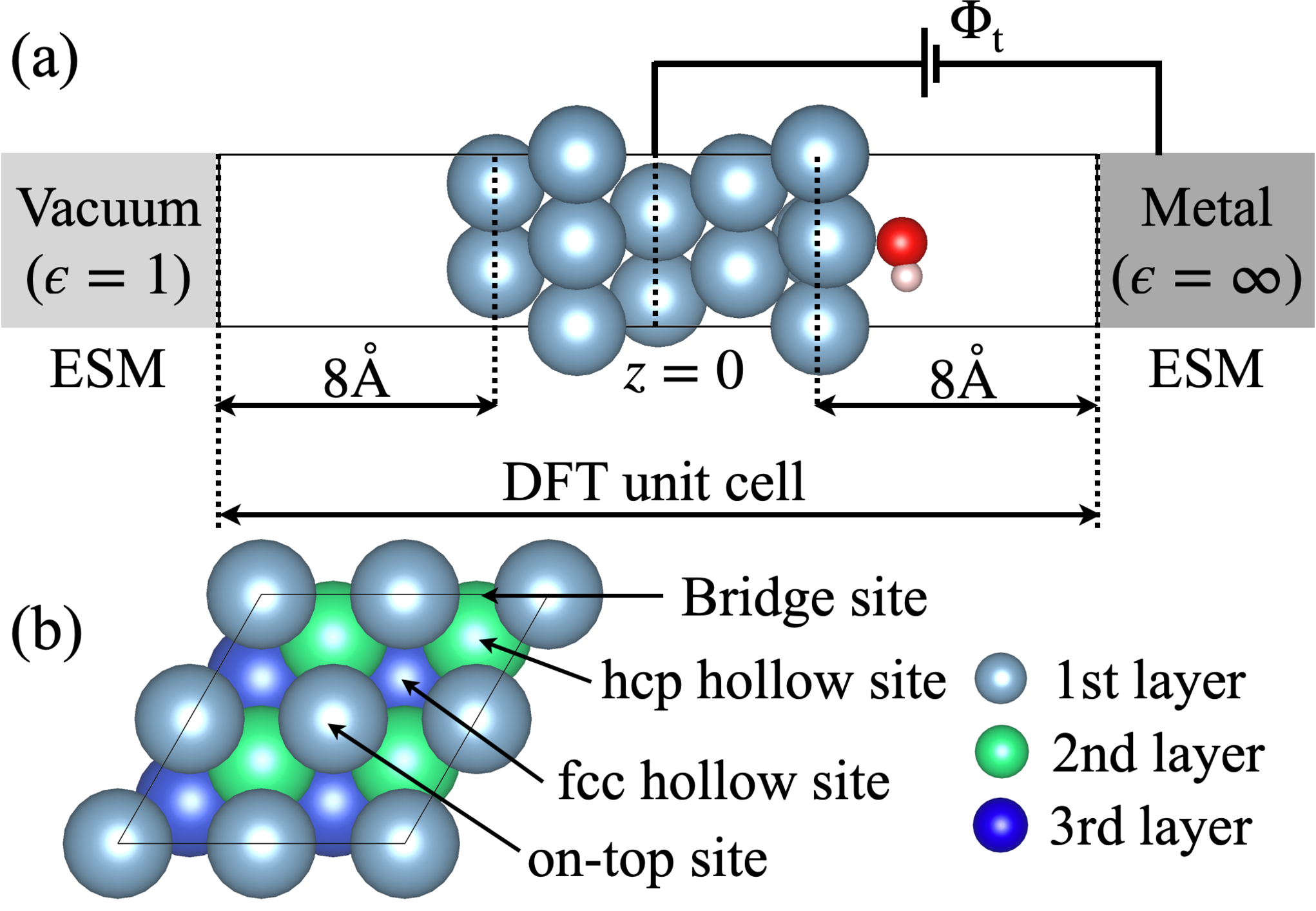
First, we briefly describe the basics of the constant-$\mu_{\mathrm{e}}$ scheme combined with the ESM method Otani and Sugino 2006. The ESM technique, which was developed by Otani and Sugino, is a powerful tool for studying various material surfaces under repeated slab approximation. Figure 1(a) shows a model of a constant-$\mu_{\mathrm{e}}$ calculation combined with the ESM used in this study. Two ESM regions with dielectric constants $\epsilon=1$ and $\epsilon=\infty$, respectively, are attached to the two ends of the supercell to represent the vacuum and the counter electrode (Metal). The electrostatic potential at the counter electrode was set to zero as the reference potential. Thus, the ESM enables us to always compare the energies measured from the same reference level.

To achieve the constant-$\mu_{\rm e}$ condition, we use the FCP Bonnet et al. 2012 and GCSCF methods Sundararaman et al. 2017. Both of these methods can be used compute the electronic structure and atomic geometry under the given target chemical potential $\mu_{\mathrm{t}}$. $\mu_{\rm t}$ is imposed by a potentiostat at a potential $\Phi_{\rm t}$, as shown in Fig. 1(a), i.e. $\mu_{\rm t}=-e\Phi_{\rm t}$, where $e$ is the charge of an electron. We can define the grand-potential $\Omega$, instead of the total energy functional $E_{\mathrm{tot}}$, as follows:

where $\Delta N_{\rm e}$ is a fictitious charge particle, which is the difference between the total number of electrons in the system $N_{\rm e}$ and that in the neutral system $N^{0}_{\rm e}$. Then, we minimize the value of $\Omega$ for the atomic positions and $\Delta N_{\rm e}$, where $\Delta N_{\rm e}$ is not a constant but a dynamic variable during the entire minimization procedure. Because both the FCP and GCSCF methods converge to the same physical state, we expect these two methods to yield the same results under the same computational conditions.

Here, we discuss the practical minimization procedure for $\Omega$ in the FCP and GCSCF methods. Figure 2(a) and (b), respectively, show the flow charts for the calculations with FCP and GCSCF, where we show a series of flows for the DFT calculation with geometry optimization. The SCF and geometry optimization loops show the blue and green shaded areas, respectively. In the following two subsections, we discuss the FCP and GCSCF methods using these flows.

Here, we provide the computational details of this study. All calculations were performed using the Quantum Espresso package Giannozzi et al. 2009; Giannozzi et al. 2017, which is a DFT code within the plane-wave basis sets and the ultrasoft-pseudopotential Vanderbilt 1990 framework. We implemented the FCP and GCSCF routines in combination with the ESM method in the package. We used the five-layered slab model in the p($2\times 2$) supercell to represent the Al(111) surface with a single water molecule, which corresponds to a 0.25 monolayer coverage, as shown in Fig. 1(a)]. The two ESM regions with $\epsilon=1$ and $\epsilon=\infty$ are located at a distance of $\sim 8~\mathrm{\AA}$ from the outermost Al layers.

For convenience, the experimental lattice constant of the face-centered cubic Al bulk ($4.05\times 4.05\times 4.05~\mathrm{\AA}^{3}$) Popović et al. 1992 was used to construct the surface slab. The cut-off energies for the wavefunctions and charge density were 40 Ry and 320 Ry, respectively. The exchange-correlation functional was the spin unpolarized version of Perdew–Wang 91 within the generalized-gradient approximation Perdew et al. 1992. $\bm{k}$-point sampling used a $5\times 5\times 1$ mesh in the surface Brillouin zone, and the number of electrons occupying the volume was determined by the Gaussian smearing method with a smearing width of 0.01 Ry. We carried out the structural optimization until $\bm{F}_{\alpha}<5.0\times 10^{-4}$ Ry/Bohr with the bottom of three Al layers fixed at bulk truncated positions. In the FCP calculation, the convergence thresholds for $\Omega$ and $F_{\rm e}$, respectively, are set to $1.0\times 10^{-6}$ Ry and $1.0\times 10^{-2}$ eV. In the GCSCF calculation, we decrease the threshold of the convergence criteria for $\Omega$ to $1.0\times 10^{-8}$ Ry, and used the Thomas–Fermi charge-mixing schemeRaczkowski et al. 2001. The NEB Henkelman et al. 2000; Henkelman and Jónsson 2000 calculation under the constant-$\mu_{\rm e}$ condition, which enables the determination of the MEP between two stable endpoints, was carried out to determine the activation barriers and diffusion paths of H₂O molecules at the surface. The NEB calculation was conducted with ten discrete images for the MEP with a path threshold of $0.03~\mathrm{eV/\AA}$. The activation barriers and diffusion paths converged well for the number of images and path threshold.

First, we briefly discuss the adsorption energy and $\mu_{\rm e}$ at the neutral Al(111) surface with a H₂O molecule for adsorption sites, as shown in Fig 1(b). The calculation shows that the on-top sites are the most stable for H₂O adsorption, and the adsorption energy we obtained for these sites is 0.23 eV. These results are consistent with the previous DFT result Ranea 2012. For the MEP, we considered H₂O diffusion from one stable on-top site to the next on-top site via a bridge site neb. To apply the bias voltage $U$, we measure $\mu_{\mathrm{t}}$ from $\mu_{\mathrm{e}}$ at the potential of zero charges (PZC), which was $-2.91$eV. In this study, $U$ is defined as $U=(\mu_{\mathrm{t}}-\mu_{\mathrm{PZC}})/e$ U_n, and the three values of $U$ are examined: $U=$ $0$V, $-1$V, and $+1$V, respectively. Here, $\mu_{\mathrm{PZC}}$ is $\mu_{\mathrm{e}}$ at the PZC.

For comparison purposes, we also carried out the constant-$N_{\mathrm{e}}$ calculations by evaluating the excess charges ($\Delta N_{\rm e}$) induced by the bias voltage. The results we obtained for $\Delta N_{\mathrm{e}}$ under $U=-1$V and $U=+1$V are $+0.033e$ and $-0.036e$, respectively. The difference in the absolute values of $\Delta N_{\rm e}$ between $U=1$V and $-1$V implies that the response of surface electrons to the applied bias potential deviates from the linear response regime. In the constant-$N_{e}$ calculation, we imposed the obtained $\Delta N_{\rm e}$ during the diffusion processes.

Table 1 presents the results of the activation barriers $E_{\mathrm{a}}$ obtained by the NEB with the constant-$\mu_{\mathrm{e}}$ and -$N_{\mathrm{e}}$ schemes. First, we briefly compare the $E_{\mathrm{a}}$ obtained by the FCP and GCSCF methods ($E^{\mathrm{FCP}}_{\mathrm{a}}$ and $E^{\mathrm{GCSCF}}_{\mathrm{a}}$). The results of $E^{\mathrm{FCP}}_{\mathrm{a}}$ are almost the same as those of $E^{\mathrm{GCSCF}}_{\mathrm{a}}$. Because the FCP and GCSCF methods converge to the same physical state, this agreement between the methods is reasonable. Hereafter, unless otherwise specified, we discuss the results of $E_{\rm a}$ using those derived with FCP as being representative of the constant-$\mu_{\rm e}$ scheme.

The result of $E_{\mathrm{a}}$ for the constant-$N_{\mathrm{e}}$ with $\Delta N_{\mathrm{e}}=0.000e$ is very close to that of the previous climbing image NEBRanea 2012. In contrast, constant-$\mu_{\mathrm{e}}$ with $U=0.0$V produces a much lower $E_{\mathrm{a}}$ compared to $E_{\mathrm{a}}$ by the constant-$N_{\mathrm{e}}$ with $\Delta N_{\mathrm{e}}=0.000e$. Under $U=-1.0$V, $E_{\mathrm{a}}$ increases to 0.161eV, which is also smaller than the counterpart value of 0.184 eV obtained with the constant-$N_{\mathrm{e}}$ scheme with $N_{\mathrm{e}}=+0.033e$. By switching the value of $U$ from $0.0$V to $+1.0$V, $E_{\mathrm{a}}$ decreases from 0.092eV to 0.024eV. $E_{\mathrm{a}}$ with $U=+1.0$V is still lower than that determined by using the constant-$N_{\mathrm{e}}$ method with $\Delta N_{\mathrm{e}}=-0.036e$. The above comparison between the constant-$\mu_{\mathrm{e}}$ and -$N_{\mathrm{e}}$ methods shows that although they yield similar trends for $E_{\mathrm{a}}$ either as a result of applying bias voltages or introducing excess charges, the results are quantitatively quite different. Compared to the previous experimental data of H₂O-diffusion Motobayashi et al. 2014, our results of $E_{\mathrm{a}}$ by the constant-$\mu_{\mathrm{e}}$ are in good agreement with the observation that the $E_{\mathrm{a}}$ of water diffusion changes significantly with respect to the bias voltage. Thus, the simulation with the constant-$\mu_{\mathrm{e}}$ method plays an important role in reproducing the experimental conditions for a constant bias-potential.

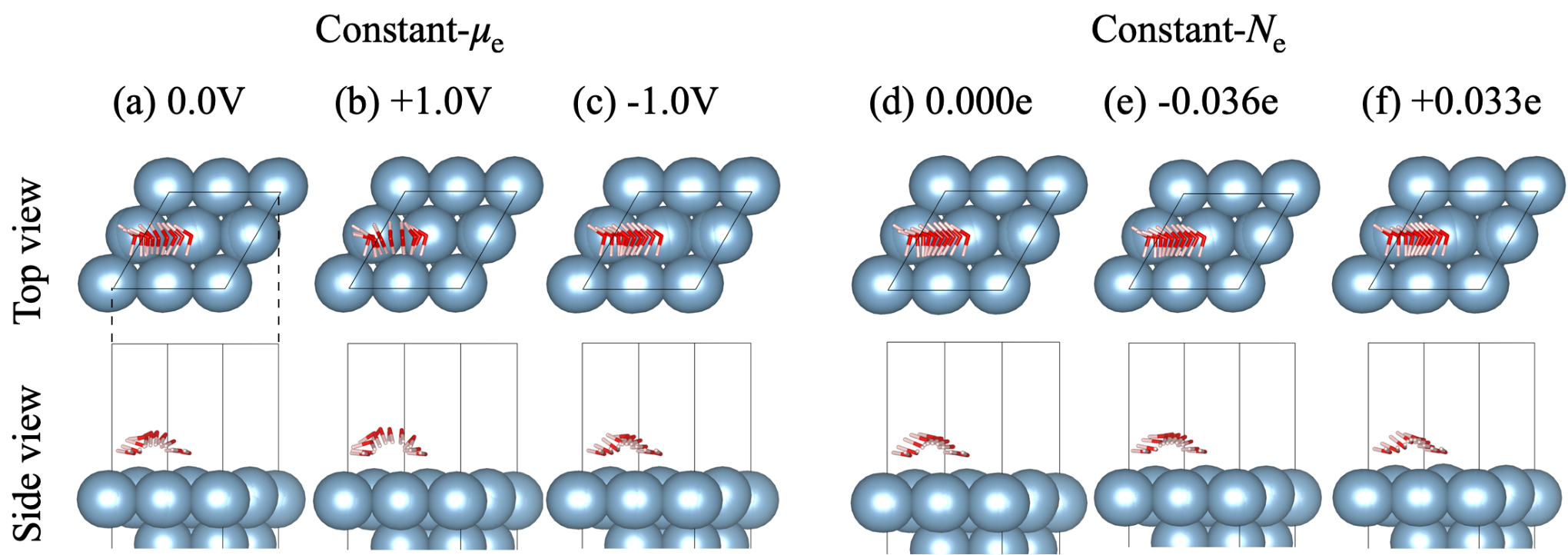
Here, we discuss the results of the water diffusion path obtained by the NEB with the constant-$\mu_{\rm e}$ and -$N_{\rm e}$ schemes. Figure 3 (a)–(c), respectively, show consecutive images of the water diffusion along the MEPs at applied bias voltage of $U=0$V, $+1.0$V, and $-1.0$V, where we show the results obtained by the FCP as a representative example. Among the ten MEP images of H₂O, we regard the first and last images as identical, and the water molecules are bonded to the surface Al atom via the O atom. Along the diffusion path, the applied bias voltage drastically alters the dipole direction of the water molecule. We can evaluate the change in the direction of the H₂O dipole by obtaining the tilt angle between the dipole normal and the surface ($\theta$). For the first H₂O image, the values of $\theta$ under $U=0.0$V, $+1.0$V, and $-1.0$V are $76^{\circ}$, $85^{\circ}$, and $71^{\circ}$, respectively. This result indicates that the changes in the adsorption structure of H₂O resulting from the bias voltage are small for the first images of MEPs. However, the value of $\theta$ changes drastically in the intermediate images as a consequence of changes in the bias voltage. The dipole direction near the bridge site at $U=0.0$V and $+1.0$V becomes nearly perpendicular to the Al surface, and the H atoms orientate themselves downward. In contrast, the dipole directions for all images tend to be parallel to the surface at $U=-1.0$V.

Figure 3(d)–(f) shows the results obtained for the MEP with the constant-$N_{\mathrm{e}}$ scheme. Here, the first and last images of H₂O in (d), (e), and (f) are the same as those in (a), (b), and (c), respectively. However, the changes in $\theta$ in the intermediate images are much smaller than those in the constant-$\mu_{\mathrm{e}}$. Thus, we interpret the difference in the results of $E_{\mathrm{a}}$ between the constant-$\mu_{\mathrm{e}}$ and -$N_{\mathrm{e}}$, as presented in Table  1, as the difference in the MEPs. Therefore, this dependence of the H₂O geometry along the MEP on the applied bias voltage indicates the importance of the interaction between the water dipole and external electric fields.

Figure 4 shows the results of the analysis with NEB. Before discussing the details of the diffusion properties, we briefly discuss the results between the FCP and GCSCF methods shown in Fig. 4(a) and (c). Overall, the results of changes in the grand-potential $\Delta\Omega$ and excess charge $\Delta N_{e}$ along the MEPs obtained by the FCP (represented by open circles) and GCSCF (represented by cross symbols) are the same within the computational accuracy. These results indicate that we successfully implemented the constant-$\mu_{\rm e}$ methods. The main difference between the FCP and GCSCF methods is the computational procedure discussed in Sec. II. Because, as discussed above, we used the extended Hessian in the FCP method, the convergence behavior depends on the inverse of the DOS near $\mu_{\mathrm{t}}$. In contrast, the GCSCF method directly optimizes $\mu_{\mathrm{e}}$ during a single SCF calculation. Because these constant-$\mu_{\mathrm{e}}$ methods employ different optimization procedures, we need to consider a different strategy to develop the FCP and GCSCF methods to more efficiently reach the constant-$\mu_{\mathrm{e}}$ condition.

Figure 4(a) presents the results of the $\Delta\Omega$, where the black, red, and blue circles, respectively, denote the values under $U=0.0$V, $-1.0$V, and $+1.0$V. In terms of the overall trend, the heights of $\Delta\Omega$ reach their respective maximum values in the intermediate images and decrease with increasing bias voltage. This behavior indicates that $E_{\mathrm{a}}$ of the diffusion of water on Al(111) depends on the external electric field, as listed in Table  1. For $U=+1.0$V, we found negative values of $\Delta\Omega$ at intermediate images of the diffusion path. This result indicates that the stable adsorption sites of the H₂O molecules on Al(111) change from the on-top sites to sites in the vicinity of the bridge sites. In contrast, the results of $\Delta E_{\mathrm{tot}}$ shown in Fig. 4(b) obtained by the constant-$N_{\rm e}$ scheme do not alter the sign of $\Delta E_{\mathrm{tot}}$ for any values of $N_{\mathrm{e}}$. Therefore, a comparison of the results of the constant-$\mu_{\mathrm{e}}$ and -$N_{\mathrm{e}}$ schemes would necessitate careful adjustment of the bias voltage to determine the stable adsorption site of H₂O on Al(111) in the STM experiments and at the electrochemical interface.

Figure 4(c) shows the results of $\Delta N_{\rm e}$ along the diffusion pathway. In the first images, the values of $\Delta N_{\rm e}$ are the same as those used in the constant-$N_{\rm e}$ calculations. In the next few images, the value of $\Delta N_{\rm e}$ increases, and then it decreases in the intermediate images of the MEPs. This result is the consequence of introducing excess charges from an external potentiostat to Al(111) to maintain a constant bias voltage. The results obtained for $\Delta\mu_{\rm e}$ by using the constant-$N_{\mathrm{e}}$ scheme highly depend on the MEPs shown in Fig. 4(d). Here, we define $\Delta\mu_{\mathrm{e}}$ as the difference between the $\mu_{\mathrm{e}}$s in the MEPs and that in the first image of the MEPs of the PZC. Because the total number of electrons is fixed, this result originates from the charge transfer between the H₂O adsorbate and the Al electrode. This charge transfer alters the height of the dipole barrier for the substrate along with the MEPs. Because the change in the surface dipole barrier alters the work function that is directly related to the electrode potential, $\Delta\mu_{\rm e}$ highly depends on the H₂O diffusion path. Thus, these differences in the control mechanism of the surface charge between the constant-$\mu_{\rm e}$ and -$N_{\rm e}$ schemes provide the different MEPs for H₂O diffusion at Al(111), as shown in Fig. 3.