Delayed Hopf bifurcation and space-time buffer curves in the Complex Ginzburg-Landau equation

Ryan Goh Affiliation: Department of Mathematics and Statistics, Boston University, Boston, MA 02215, USA Tasso J. Kaper Affiliation: Department of Mathematics and Statistics, Boston University, Boston, MA 02215, USA Theodore Vo Affiliation: School of Mathematics, Monash University, Clayton, Victoria 3800, Australia

Abstract

In this article, the recently-discovered phenomenon of delayed Hopf bifurcations (DHB) in reaction-diffusion PDEs is analyzed in the cubic Complex Ginzburg-Landau equation, as an equation in its own right, with a slowly-varying parameter. We begin by using the classical asymptotic methods of stationary phase and steepest descents to show that solutions which have approached the attracting quasi-steady state (QSS) before the Hopf bifurcation remain near that state for long times after the instantaneous Hopf bifurcation and the QSS has become repelling. In the complex time plane, the phase function of the linear PDE has a saddle point, and the Stokes and anti-Stokes lines are central to the asymptotics. The nonlinear terms are treated by applying an iterative method to the mild form of the PDE given by perturbations about the linear particular solution. This tracks the closeness of solutions near the attracting and repelling QSS. Next, we show that beyond a key Stokes line through the saddle there is a curve in the space-time plane along which the particular solution of the linear PDE ceases to be exponentially small, causing the solution of the nonlinear PDE to diverge from the repelling QSS and exhibit large-amplitude oscillations. This curve is called the space-time buffer curve. The homogeneous solution also stops being exponentially small in a spatially dependent manner, as determined also by the initial time. Hence, a competition arises between these two solutions, as to which one ceases to be exponentially small first, and this competition governs spatial dependence of the DHB. We find four different cases of DHB, depending on the outcomes of the competition, and we quantify to leading order how these depend on the main system parameters, including the Hopf frequency, initial time, initial data, source terms, and diffusivity. Examples are presented for each case, with source terms that are uni-modal, spatially-periodic, smooth step function, and algebraically-growing. Also, rich spatio-temporal dynamics are observed in the post-DHB oscillations. Finally, it is shown that large-amplitude source terms can be designed so that solutions spend substantially longer times near the repelling QSS, and hence region-specific control over the delayed onset of oscillations can be achieved.

Keywords Slow passage through Hopf bifurcation, dynamic bifurcation in PDEs, spatially-inhomogeneous onset of oscillations, hard onset of oscillations, stationary phase method, steepest descents method, complex Ginzburg-Landau equation, reaction-diffusion equations

1 Introduction

In applied mathematics, physics, biology, and in many other areas of science and engineering, the phenomenon of delayed Hopf bifurcation (DHB) is a central feature of analytic ordinary differential equations (ODEs) in which a parameter passes slowly through a Hopf point. ODE models and experimental examples arise in chemistry and pattern formation [9, 22, 23, 38, 39, 61], nonlinear mechanical oscillators and generalised Rayleigh oscillators [13, 51, 52], electrical engineering [29, 67], fluid dynamics and geophysics [2, 21, 32, 44], neuroscience [7, 10, 11, 12, 16, 25, 26, 35, 55, 56, 59, 62, 63], cardiac models [40], and the Kaldor model in business [27].

In DHB for ODEs, the key system parameter passes slowly in time through a Hopf bifurcation value at which the stable equilibrium becomes unstable, yet the solutions remain near the repelling equilibrium for long times, of length $\mathcal{O}(1)$ in the slow time, after the Hopf point. As a result, in the super-critical case, the attendant (post-DHB) onset of oscillations is a hard onset, with solutions jumping rapidly away from the unstable equilibrium to the stable limit cycle, which by that time already has a large amplitude. DHB has been studied in analytic ODEs for more than 50 years, going back at least to the seminal work [58]. The theory is further developed in [5, 22, 31, 33, 47, 48, 62], and is also presented in recent monographs [41, 66]. Moreover, many of the above applications have been inspired by [5, 47, 48].

DHB has also been studied [11] in large systems of ODEs. There, the FitzHugh-Nagumo and Hodgkin-Huxley cable equations are studied with a slowly varying Neumann boundary condition at one end of the spatial domain and a zero-flux condition at the other end. The spatial variable in these partial differential equations (PDEs) is discretised (with centered finite differences for the Laplacian), and the WKB method is used to analyze DHB in the large system of ODEs.

Recently, it was discovered that the phenomenon of DHB also occurs in reaction-diffusion equations [36]. In that work, it was shown using numerics, physical considerations, and some Fourier analysis that DHB is important for a variety of reaction-diffusion equations in which there is slow passage through super-critical Hopf bifurcations. The reaction-diffusion examples in which DHB has been found [36] include the Complex Ginzburg-Landau equation, the Brusselator model of the Belousov-Zhabotinsky reaction, the Hodgkin-Huxley PDE, the FitzHugh-Nagumo PDE, and a spatially-extended pituitary lactotroph cell model.

There has been rigorous analysis in [3] of spatio-temporal canards and delayed bifurcations in a class of infinite-dimensional systems on bounded domains, which includes slow passage through Hopf bifurcation, slow passage through a Turing bifurcation, and some bifurcations in delay-differential equations. In that article, under the assumption that a spectral gap exists in the fast sub-system, a center manifold analysis is performed using the infinite-dimensional invariant manifold theory of Haragus and Iooss [30]. See also the references in [3, 65] for more on spatio-temporal canards.

In this article, we use the methods of stationary phase and steepest descents to analyze the DHB created when the bifurcation parameter $\mu$ slowly increases through a supercritical Hopf bifurcation (at zero) in the Complex Ginzburg Landau equation on the real line,

\begin{split}A_{t}&=(\mu+i\omega_{0})A-(1+i\alpha)|A|^{2}A+\eps^{\beta}I_{a}(x)+\eps^{\gamma}dA_{xx}\\ \mu_{t}&=\eps.\end{split}

(1.1)

Here, $x$ is real, $t\geq 0$ , $A=A(x,t)$ is complex-valued, and $0<\eps\ll 1$ is a small parameter. The linear growth rate $\mu=\mu(t)$ is real for the main phenomena we study; however, for the mathematical analysis, it will be advantageous to consider complex values of $\mu$ in a horizontal strip with mid-line on the real axis and of sufficient height. The system parameters satisfy $\omega_{0}>0$ and $\mathcal{O}(1)$ independent of $\eps$ , $\alpha$ is real, $\beta>0$ , $\gamma\geq 0$ , $d$ may be complex-valued ( $d=d_{R}+id_{I}$ ) with $d_{R}>0$ , and they are independent of $\eps$ . For real values of $x$ , the source term $I_{a}(x)$ , which breaks the symmetry $A\to Ae^{i\theta}$ for any real $\theta$ of the CGL equation, is typically taken to be bounded and positive, with uniformly bounded derivatives. The initial data at $\mu(0)=\mu_{0}<0$ is $A(x,0)=A_{0}(x)$ , and typically taken to be bounded and continuous for all real $x$ . Also, it will be useful to distinguish between initial data given at $\mu_{0}\leq-\omega_{0}$ and data given at $-\omega_{0}<\mu_{0}<0$ .

The PDE (1.1) has an attracting Quasi-Steady State (QSS) for all $\mu<-\delta$ , where $\delta>0$ , small, and $\mathcal{O}(1)$ , which solutions approach at an exponential rate. Similarly, it has a repelling QSS for all $\mu>\delta$ , from which solutions diverge at an exponential rate. For example, in the base case of $\beta=\frac{1}{2}$ and $\gamma=1$ , the attracting QSS (for $\mu<-\delta$ ) and the repelling QSS (for $\mu>\delta$ ) are given by

A_{\rm QSS}(x,\mu)=-\sqrt{\eps}\frac{I_{a}(x)}{\mu+i\omega_{0}}+\eps^{\frac{3}{2}}\left(\frac{I_{a}(x)+d(\mu+i\omega_{0}){I_{a}}^{\prime\prime}(x)}{(\mu+i\omega_{0})^{3}}-\frac{(1+i\alpha)I_{a}^{3}(x)}{(\mu+i\omega_{0})^{2}(\mu^{2}+\omega_{0}^{2})}\right)+\mathcal{O}(\eps^{\frac{5}{2}}).

(1.2)

Here, the $\mathcal{O}(\eps^{\frac{5}{2}})$ terms depend on $x$ and $\mu$ . The QSS may also be derived for other $\beta$ and $\gamma$ .

In [36], DHB is observed for solutions which are in a fixed $\mathcal{O}(1)$ neighbourhood of the attracting QSS for any $\mu_{0}$ sufficiently negative. These solutions all continue to approach the attracting QSS until $\mu=0$ , where the instantaneous Hopf bifurcation occurs. However, rather than immediately tracking the stable (post-DHB) oscillatory state as it grows in amplitude, these solutions remain near the repelling QSS for long times into $\mu>0$ . Moreover, the amount of time any such solution $A(x,t)$ spends near the repelling QSS can, and generally does, depend on $x$ . See Figure 1.

Refer to caption — Figure 1: DHB in the PDE (1.1) in the base case of $\beta=\frac{1}{2}$ and $\gamma=1$ , with a Gaussian source term $I_{a}(x)=e^{-\frac{x^{2}}{4}}$ on the domain $[-\ell,\ell]$ ( $\ell=30$ ). The solution is near the attracting QSS while $\mu\in[\mu_{0},0)$ (with $\mu_{0}=-1$ , not shown). Then, for $\mu>0$ , i.e., after the instantaneous Hopf bifurcation, the solution stays near the repelling QSS (green state) at least until $\mu=\omega_{0}=0.5$ at all points $x$ . The duration of the DHB (i.e., the length of time the solution stays near the repelling QSS) is spatially dependent. At $x=0$ , $A(x,\mu)$ first leaves a neighbourhood of the repelling QSS at time $\mu=\omega_{0}$ , and the large-amplitude oscillations first set in there. Then, as one steps outward from the center, with $|x|>0$ , the duration of the DHB grows beyond $\mu=\omega_{0}$ . The hard onset of the large-amplitude oscillations is governed to leading order by the space-time buffer curve studied in this article. Here, $\eps=0.01,\omega_{0}=\tfrac{1}{2},d_{R}=1,d_{I}=0,$ and $\alpha=0$ .

Our first goal in this article is to derive a general formula for the space-time buffer curve of system (1.1) with general source terms $I_{a}(x)$ . The space-time buffer curve corresponds to the $x$ -dependent (post-DHB) time at which the solution cannot remain near the repelling QSS any longer for each point $x$ , irrespective of how far before the slowly-varying Hopf point the solution was attracted to the (pre-Hopf) stable QSS. We directly to leading order apply the classical methods of stationary phase and steepest descents (see for example [8, 37, 46]) to the linear CGL equation, obtained by linearising (1.1) about $A=0$ . The coefficient $(\mu+i\omega_{0})$ on the linear homogeneous term vanishes at $\mu=-i\omega_{0}$ in the complex $\mu$ plane. This is a saddle point of the complex phase $-\frac{1}{2}(\mu+i\omega_{0})^{2}$ , since the derivative of the phase vanishes there. Moreover, the lines of stationary phase of the linear PDE through this saddle point, along which the real part of the phase vanishes, are given by $\mu_{I}=\pm\mu_{R}-\omega_{0}$ , where $\mu=\mu_{R}+i\mu_{I}$ . In the vicinity of the saddle, analysis along the relevant Stokes and anti-Stokes lines shows that all solutions with initial data at $\mu_{0}\leq-\omega_{0}$ stay near the attracting QSS while $\mu$ is negative and then, also, that they stay near the repelling QSS at all points $x$ at least until $\mu$ reaches $+\omega_{0}$ , to leading order. More importantly, application of the methods of stationary phase and steepest descents yields the formula for the space-time buffer curve, $(\mu_{\rm stbc}(x),x)$ with $\mu_{\rm stbc}(x)\geq\omega_{0}$ for all $x$ , for the general class of source terms considered here. This space-time buffer curve represents the $x$ -dependent times at which the particular solution of the linearised PDE ceases to be exponentially small, and at which the hard onset of oscillations occurs, to leading order. Similarly, there is a homogeneous exit time curve, $\mu_{h}(x)$ , along which the homogeneous component of the PDE has magnitude one. Therefore, it is important to determine, at each point $x$ , which of the two times $\mu_{\rm stbc}(x)$ and $\mu_{h}(x)$ is smaller, causing the solution of the full cubic PDE to stop being exponentially small first. The smaller of the two times marks the duration of the DHB, to leading order.

After completing this first goal, we study how the properties of DHB depend on the outcome of this competition between $\mu_{\rm stbc}(x)$ and $\mu_{h}(x)$ , as well as on the properties of $I_{a}(x)$ . For solutions with initial data given at any $\mu_{0}\leq-\omega_{0}$ , we identify three cases of DHB: one in which the particular solution determines the onset of oscillations at all $x$ in the domain; another case in which the time of onset is determined by the particular solution for some intervals on the domain and by the homogeneous solution on the complementary intervals; and, a third case in which the homogeneous solution determines the exit time at all points. We examine spatially uni-modal, spatially periodic, and smoothed step function source terms. In these examples, quantitative agreement is found between the leading order analysis in all cases of DHB and the results of direct numerical simulations of (1.1) with zero-flux boundary conditions on $[-\ell,\ell]$ and all values of $\ell$ for which simulations were conducted. Balanced symmetric Strang operator splitting [60] was used, with centered finite differences for the Laplacian and fourth-order Runge-Kutta for the time-stepping.

In addition, we show that solutions of (1.1) can exhibit spatially-dependent DHB also when the initial data is given at times $\mu_{0}\in(-\omega_{0},-\delta]$ for some small $\delta>0$ . We label this as Case 4 of DHB. For these solutions with initial data given at times much closer to the time of the instantaneous Hopf bifurcation, the spatial dependence of $\mu_{h}(x)$ causes the exit time from a neighborhood of the repelling QSS to be asymmetric about $\mu=0$ with respect to the time of entry into a neighborhood of the attracting QSS. This contrasts with the dynamics of DHB in analytic ODEs, where the entry-exit function (also known as the way-in way-out function) is symmetric for initial conditions given close to the instantaneous Hopf bifurcation.

After having carried out the analysis of DHB in the above four cases, we use a formal analysis to show that solutions of the full, cubic CGL equation (1.1) with initial data given at time $\mu_{0}\leq-\omega_{0}$ are also close to the attracting QSS (now of the full nonlinear PDE) on $\mu<0$ and remain close to the repelling QSS after the instantaneous Hopf bifurcation ( $\mu=0$ ) at least until $\mu=\omega_{0}$ in Case 1 of DHB. The nonlinear analysis is carried out using the integral form of the equation governing the difference between the solution of the full nonlinear PDE and the particular solution of the linear PDE. Use of an iterative method then establishes the closeness to the repelling QSS in the cubic PDE, and it reveals how the asymptotic expansion of the QSS is naturally generated. The main result is that, to leading order, solutions of the cubic CGL (1.1) stay near the repelling QSS until the same space-time buffer curve in Case 1 of DHB. Moreover, we note that, the situation here for DHB in the CGL PDE is similar in this respect to that for DHB in analytic ODEs, where the linear problem determines the buffer point to leading order in the ODEs, and the nonlinear terms in the analytic ODE (such as the cubic term $-|A|^{2}A$ ) only contribute at higher order to DHB.

Finally, we extend the main DHB results for the base case of the PDE (1.1) in several directions. The simplest extension is to take into account the higher order terms in the instantaneous Hopf bifurcation curve for the base case. To leading order, this curve is given by $\mu=0$ in the space-time plane. The first non-zero correction occurs at $\mathcal{O}(\eps)$ , and we will study its impact on DHB. As a second extension, we study the DHB also in the base case but now with source terms which do not satisfy the hypotheses imposed on $I_{a}(x)$ in the general analysis, namely with an algebraically-growing and a sign-changing function. Nevertheless, for each of these sources, we also find good agreement between the analytically calculated space-time buffer curve and the numerically calculated spatially-dependent times at which the solutions leave a neighborhood of the repelling QSS and the oscillations set in for the nonlinear PDE (1.1).

In a third direction, we extend the analysis of the base case to asymptotically large-amplitude ( $\beta=-\frac{1}{2}$ ) source terms in the PDE (1.1), while retaining small diffusivity ( $\gamma=1$ ). Here, the QSS are highly-nontrivial, and the instantaneous Hopf bifurcation times are spatially dependent, instead of being homogeneous at $\mu=0$ , to leading order. We explore the more complex spatial dependence of the Hopf bifurcation curve and the space-time buffer curve. An example shows that it is possible to choose the amplitude and form of the large source term (and hence of the resulting QSS) to design even more complex spatio-temporal onset of oscillations, giving region-specific control over the onset of oscillations. In a fourth direction, we briefly extend the analysis of the base case to an example with $\mathcal{O}(1)$ diffusivity and $\mathcal{O}(1)$ amplitude source term, (i.e., $\gamma=0$ and $\beta=0$ in (1.1)). The space-time buffer curve gets somewhat flattened out compared to the case of $\mathcal{O}(\eps)$ diffusivity.

While our primary motivation is to carry out this analysis of DHB in the CGL PDE (1.1) and to derive a method that can be used on other reaction-diffusion (R-D) systems known to exhibit DHB [36], another motivation for understanding the phenomenon of DHB in PDEs is that some ODE models exhibiting DHB are simplified versions or conceptual models of more complex phenomena which involve diffusion and advection. An example is the Maasch-Saltzman ODE model of glacial cycles [44], in which DHB is advanced as a possible mechanism for the mid-Pleistocene transition from 40,000 year glacial cycles to approximately 100,000 year cycles. See also [21]. Since the Maasch-Saltzman model is a useful conceptual ODE model, one would also like to know whether or not the corresponding PDE models, such as a more fully developed PDE model of the Pleistocene glacial cycles, can also exhibit DHB. Otherwise, for these problems, the phenomenon of DHB would only be of more limited interest. Along with [3, 36], this work presents a step in that larger direction, showing that DHB also occurs in nonlinear spatially-extended systems.

We observe that the analysis presented herein builds naturally on the results known about DHB in analytic ODEs. In fact, in the case of $d=0$ and a spatially-homogeneous source term $I_{a}(x)\equiv I_{a}$ , system (1.1) reduces to a prototypical form of DHB in analytic ODEs. In this case, we directly recover the known DHB results for analytic ODEs, see [5, 31, 47, 48, 58]. The hard onset of oscillations occurs to leading order at the buffer point $\mu=\omega_{0}$ of the ODEs, and it is spatially uniform. An example is provided by the Shishkova equation, $\eps z_{\mu}=(\mu+i\omega_{0})z-(1+i\alpha)|z|^{2}z+\eps h(\mu)$ for $z(\mu;\eps)$ , with $h(-i\omega_{0})\neq 0$ and $0<\eps\ll 1$ . See [58]. This equation has a family of attracting slow invariant manifolds for $\mu<-\delta$ , where $\delta>0$ is small and independent of $\eps$ , and a family of repelling slow invariant manifolds for $\mu>\delta$ . These families of manifolds may be extended in to the regions $\mu>0$ and $\mu<0$ , respectively, and they are exponentially close to each other on $(-\omega_{0},\omega_{0})$ to leading order. By the theory of DHB in ODEs, any solution which enters a fixed, small neighbourhood of an attracting slow invariant manifold at a value of $\mu<-\omega_{0}$ must exit a neighbourhood of the repelling slow invariant manifold at $\mu=\omega_{0}$ to leading order, which is the buffer point. This delayed loss of stability occurs at $\mu=\omega_{0}$ (to leading order) for these solutions independently of how much time they have spent spiraling in toward the attracting manifold before $\mu$ reaches $-\omega_{0}$ . This is because the term $\eps h(\mu)$ breaks the symmetry of $z\to-z$ in the Shishkova equation and because the intersection at $\mu=\omega_{0}$ of the Stokes line through the saddle (or nilpotent) point at $\mu=-i\omega_{0}$ with the real axis acts as a barrier, or buffer point. Hence, all solutions that have been attracted to that slow manifold must diverge away from the repelling manifold along with it, irrespective of how far back in the past they approached the attracting manifold.

Finally, we remark that, just as is observed here, lines of stationary phase and lines of steepest ascents and descents play central roles in the asymptotics of solutions of many linear and nonlinear ODEs and PDEs. For the general theory of the Stokes phenomenon, see for example [8, 14, 15, 18, 20, 37, 45, 46, 50]. We follow naming conventions in [8, 37, 46]. Moreover, in many of these equations, there are multiple components which cease to be exponentially small, by crossing Stokes lines for example, and which transition through modulus one to becoming large.

This article is organised as follows. In Section 2, the linear CGL equation is studied in the base case of (1.1) with $\beta=1/2$ and $\gamma=1$ , establishing that solutions with $\mu_{0}<-\omega_{0}$ remain near the attracting and repelling QSSs at least until $\mu=+\omega_{0}$ for all $x$ . In Section 3, the space-time buffer curve $(\mu_{\rm stbc}(x),x)$ is derived, where $\mu_{\rm stbc}(x)\geq\omega_{0}$ for bounded, positive source terms, showing that DHB occurs in the CGL PDE. Also, the examples of different $I_{a}(x)$ are given to show how their extrema and spatial form (uni-modal, periodic, smoothed step function) determine the location of the space-time buffer curve and the dynamics of DHB. In Section 4, we examine the homogeneous solutions and derive the homogeneous exit time curve, $\mu_{h}(x)$ . This establishes the spatially-dependent exit times caused by the homogeneous components of the linear solutions, both when the initial data is given at a time $\mu_{0}\leq-\omega_{0}$ , and when it is given at a time $\mu_{0}\in(-\omega_{0},0)$ . In Section 5, the four cases of DHB are classified, with examples. In Section 6, the analysis of the nonlinear PDE is presented, establishing the closeness of the solutions to the repelling QSS of the full cubic CGL equation. In Section 7, it is shown how the DHB of the solutions of (1.1) is influenced by the $\mathcal{O}(\eps)$ terms in the time of the instantaneous Hopf bifurcation. In Section 8, examples are presented with algebraically-growing and sign-changing source terms, to push beyond the analysis of the general system. Then, the impact of the large-amplitude source terms ( $\beta=-1/2$ ) is analyzed in Section 9. Also, the extension of the DHB results and space-time buffer curve formula to the case of $\mathcal{O}(1)$ diffusivity ( $\gamma=0$ ) and amplitude source term ( $\beta=0$ ) is given in Section 10. Conclusions and discussion are presented in Section 11.

2 Linear analysis for solutions with $\mu_{0}<-\omega_{0}$

In this section, we analyze the linear CGL equation, obtained by linearising (1.1) about $A=0$ , in the base case of moderate-amplitude source terms ( $\beta=\frac{1}{2}$ ) and small-amplitude diffusivity ( $\gamma=1$ ),

\begin{split}A_{t}&=(\mu+i\omega_{0})A+\sqrt{\eps}I_{a}(x)+\eps dA_{xx}\\ \mu_{t}&=\eps.\end{split}

Equivalently, the system may be written as a scalar equation for $A(x,\mu)$ ,

\eps A_{\mu}=(\mu+i\omega_{0})A+\sqrt{\eps}I_{a}(x)+\eps dA_{xx}.

(2.1)

Here, $\mu(t)=\mu_{0}+\eps t$ , and we focus on data for which $\mu_{0}\leq-\omega_{0}$ . The other case, with data given at a time $\mu_{0}\in(-\omega_{0},0)$ , is analyzed in Section 4.

For $0<\eps\ll 1$ , all solutions with $\mu_{0}\leq-\omega_{0}$ rapidly and exponentially approach an attracting QSS, see (1.2) (which also contains the terms in the QSS for the full nonlinear equation), since the real part of the coefficient on the linear term is negative and stays well bounded away from zero for these $\mu<0$ . In this section, we show that the solutions with $\mu_{0}\leq-\omega_{0}$ not only remain close to the attracting QSS until the time of the instantaneous Hopf bifurcation, but after the parameter crosses the instantaneous Hopf bifurcation at $\mu=0$ they remain close to the repelling QSS as well, at least until the time $\mu=+\omega_{0}$ at all points $x$ for the functions $I_{a}(x)$ we study. This will be shown using the classical methods of stationary phase and steepest descents, see [8, 37, 46].

2.1 The homogeneous and particular solutions

Define the following new dependent variable, which is based on an integrating factor,

B(x,\mu)=A(x,\mu)e^{-\frac{1}{2\eps}(\mu+i\omega_{0})^{2}}.

(2.2)

Equation (2.1) may then be written as

\sqrt{\eps}B_{\mu}=I_{a}(x)e^{-\frac{1}{2\eps}(\mu+i\omega_{0})^{2}}+\sqrt{\eps}dB_{xx}.

(2.3)

By Duhamel’s Principle, the solution consists of homogeneous and particular components,

B(x,\mu)=B_{h}(x,\mu)+B_{p}(x,\mu).

(2.4)

The homogeneous component satisfies $(B_{h})_{\mu}=d(B_{h})_{xx}$ with $B_{h}(x,\mu_{0})=A_{0}(x)$ ,

B_{h}(x,\mu)=\frac{e^{-\frac{1}{2\eps}(\mu_{0}+i\omega_{0})^{2}}}{\sqrt{4\pi d(\mu-\mu_{0})}}\int_{\mathbb{R}}e^{\frac{-(x-y)^{2}}{4d(\mu-\mu_{0})}}A_{0}(y)dy.

(2.5)

This homogeneous solution is valid (at least) for all real $\mu>\mu_{0}$ , recalling that $\mu_{0}<-\omega_{0}$ , and throughout this article, we will evaluate or estimate it on the ${\rm Re}(\mu)$ -axis. Nevertheless, we note that, with the initial data used in the examples, $B_{h}(x,\mu)$ is actually analytic in the complex $\mu$ plane, excluding the branch point and cut. Note that, for general initial data, $A_{0}(x)$ is Gevrey regular of order $k=\frac{1}{2}$ on an appropriate domain implies that the homogeneous solution $A_{h}(x,\mu)$ is analytic, by standard theory for homogeneous heat equations. See for example [54], and recall that a function $f(z)$ is Gevrey regular of order $k$ on a set $|z|<r$ , if there exist positive constants $C_{1},C_{2}$ such that ${\rm max}_{|z|\leq r}|\frac{d^{k}f}{dz^{k}}(z)|\leq C_{1}C_{2}^{k}(k!)^{\frac{1}{2}}$ .

The particular solution satisfies the full linear PDE (2.3), but with zero initial condition at $\mu_{0}$ ,

\begin{split}B_{p}(x,\mu)&=\frac{1}{\sqrt{\eps}}\int_{\mu_{0}}^{\mu}g(x,\mu-\tilde{\mu})e^{-\frac{1}{2\eps}(\tilde{\mu}+i\omega_{0})^{2}}d\tilde{\mu},\\ g(x,\mu-\tilde{\mu})&=\frac{1}{\sqrt{4\pi d(\mu-\tilde{\mu})}}\int_{\mathbb{R}}e^{\frac{-(x-y)^{2}}{4d(\mu-\tilde{\mu})}}I_{a}(y)dy.\end{split}

(2.6)

The source terms $I_{a}(x)$ we study are such that $g(x,\mu-{\tilde{\mu}})$ is analytic in a region of the complex plane which includes the portion of the real axis with $\mu>{\tilde{\mu}}$ , but which excludes a small neighborhood of the branch point and cut. Then, in turn, $B_{p}(x,\mu)$ is analytic in an appropriate region about the segment $(\mu_{0},\omega_{0})$ of the ${\rm Re}(\mu)$ -axis. For more general source terms, one needs to require that $I_{a}(x)$ is Gevrey regular of order $k=\frac{1}{2}$ in a region containing a segment of the ${\rm Re}(x)$ -axis, sufficiently large to guarantee that $B_{p}(x,\mu)$ is analytic in $\mu$ for ${\rm Re}(\mu)>{\rm Re}({\tilde{\mu}})$ . This follows from standard theory for the analyticity of solutions. We refer to [6, 43, 54] for the general theory of analyticity of solutions and Gevrey regularity of order $k$ for homogeneous and inhomogeneous heat equations.

In the complex ${\tilde{\mu}}$ plane ( ${\tilde{\mu}}={\tilde{\mu}}_{R}+i{\tilde{\mu}}_{I}$ ), the phase function in the integrand of $B_{p}$ is

-\frac{1}{2}({\tilde{\mu}}+i\omega_{0})^{2}=\phi+i\psi,\ \ {\rm where}\ \ \phi=-\frac{1}{2}\left({\tilde{\mu}}_{R}^{2}-({\tilde{\mu}}_{I}+\omega_{0})^{2}\right)\ \ {\rm and}\ \ \psi=-{\tilde{\mu}}_{R}({\tilde{\mu}}_{I}+\omega_{0}).

(2.7)

This phase has a saddle point at ${\tilde{\mu}}=-i\omega_{0}$ , and the topography induced by this saddle will play a central role in the analysis. The level sets of $\phi$ are hyperbolas and also known as Stokes lines. The Stokes lines with $\phi=0$ through the saddle (which are the asymptotes of the hyperbolas) bound the valleys and hills. They may be parametrised by ${\tilde{\mu}}_{R}$ via ${\tilde{\mu}}_{I}=\pm{\tilde{\mu}}_{R}-\omega_{0}.$ Also, the level sets of $\psi$ are hyperbolas (with asymptotes given by the axes), and they are referred to as anti-Stokes lines. The geometry is illustrated in Figure 2. See [8, 18, 37, 46], for example, for the general theory of Stokes and anti-Stokes lines.

Remark. The integral involving $A_{0}(y)$ in (2.5) is the same as the integral involving $I_{a}(y)$ in (2.6)(b), in the case when $A_{0}(y)$ is chosen as a multiple of $I_{a}(y)$ and with $\mu_{0}$ replacing ${\tilde{\mu}}$ .

2.2 Tracking the particular solutions near the attracting QSS

In this section, we briefly show using steepest descents that solutions with $\mu_{0}\leq-\omega_{0}$ stay near the attracting QSS before the instantaneous Hopf bifurcation. Although the result is of course well known, it is useful to demonstrate briefly how the asymptotic method of steepest descents naturally finds the asymptotic expansion of the attracting QSS.

Let $\delta>0$ be sufficiently small and independent of $\eps$ . We fix an arbitrary value of $\mu\in(-\omega_{0},-\delta]$ , and track the particular solution $B_{p}$ from $\mu_{0}$ to the fixed value $\mu$ . Let $C_{a}$ denote the contour $C_{a1}\bigcup C_{a2}$ , where $C_{a1}$ consists of the semi-infinite segment of the steepest descent curve $\psi\equiv-\omega_{0}\mu_{0}$ from the point $\mu_{0}$ on the real axis out to infinity ( $-\infty-i\omega_{0}$ ) toward the horizontal asymptote ${\tilde{\mu}}_{I}=-\omega_{0}$ , and $C_{a2}$ consists of the semi-infinite segment of the steepest ascent curve $\psi\equiv-\omega_{0}\mu$ from infinity back up to the fixed value $\mu$ on the real axis. Note that $C_{a2}$ crosses the Stokes line $\mu_{I}=-\mu_{R}-\omega_{0}$ at the point $q_{a}=-\sqrt{-\omega_{0}\mu}+i(\sqrt{-\omega_{0}\mu}-\omega_{0})$ . See Figure 2.

We track $B_{p}$ along $C_{a}$ from $\mu_{0}$ to the fixed value $\mu$ on $(-\omega_{0},-\delta]$ . By (2.6), the solution is

\begin{split}B_{p}(x,\mu)&=\mathcal{I}_{a1}+\mathcal{I}_{a2},\quad{\rm where}\\ \mathcal{I}_{ai}&=\frac{1}{\sqrt{\eps}}\int_{C_{ai}}g(x,\mu-{\tilde{\mu}})e^{-\frac{1}{2\eps}({\tilde{\mu}}+i\omega_{0})^{2}}d{\tilde{\mu}},\ \ i=1,2,\qquad\mu\in(-\omega_{0},-\delta].\end{split}

(2.8)

Directly from $\phi$ , the real part of the complex phase (2.7), and the analyticity of $g$ , one finds

|\mathcal{I}_{a1}|\leq Ce^{-\frac{1}{2\eps}(\mu_{0}^{2}-\omega_{0}^{2})},\quad{\rm for}\ {\rm some}\ C>0.

(2.9)

The main work then is to derive the result for $\mathcal{I}_{a2}$ , which we do using two different parametrisations of $C_{2}$ , explicitly here using ${\tilde{\mu}}_{R}$ , and implicitly in Appendix A,

C_{a2}:\quad{\tilde{\mu}}={\tilde{\mu}}_{R}+i{\tilde{\mu}}_{I}({\tilde{\mu}}_{R}),\quad{\rm with}\ \ {\tilde{\mu}}_{I}({\tilde{\mu}}_{R})=-\omega_{0}\left(1-\frac{\mu}{{\tilde{\mu}}_{R}}\right).

(2.10)

Along $C_{a2}$ , ${\tilde{\mu}}_{R}$ increases from $-\infty$ to $\mu$ , and ${\tilde{\mu}}_{I}$ increases from $-\omega_{0}$ to zero. Also, we observe that, by (2.10), $\frac{d{\tilde{\mu}}}{d{\tilde{\mu}}_{R}}=1-\frac{i\omega_{0}\mu}{{\tilde{\mu}}_{R}^{2}}$ . Hence,

\mathcal{I}_{a2}=\frac{1}{\sqrt{\eps}}\int_{-\infty}^{\mu}g\left(x,\mu-{\tilde{\mu}}_{R}+i\omega_{0}\left(1-\frac{\mu}{{\tilde{\mu}}_{R}}\right)\right)e^{-\frac{1}{2\eps}\left({\tilde{\mu}}_{R}+i\frac{\omega_{0}\mu}{{\tilde{\mu}}_{R}}\right)^{2}}\left(1-\frac{i\omega_{0}\mu}{{\tilde{\mu}}_{R}^{2}}\right)d{\tilde{\mu}}_{R}.

Now, it is useful to define

u({\tilde{\mu}}_{R})=-\eps\frac{g\left(x,\mu-{\tilde{\mu}}_{R}+i\omega_{0}\left(1-\frac{\mu}{{\tilde{\mu}}_{R}}\right)\right)}{\left({\tilde{\mu}}_{R}+\frac{i\omega_{0}\mu}{{\tilde{\mu}}_{R}}\right)}\qquad v({\tilde{\mu}}_{R})=e^{-\frac{1}{2\eps}\left({\tilde{\mu}}_{R}+i\frac{\omega_{0}\mu}{{\tilde{\mu}}_{R}}\right)^{2}}.

(2.11)

Hence, using integration by parts, formula (2.6)(b) for $g$ , and $\lim_{\chi\to 0^{+}}g(x,\chi)=I_{a}(x)$ , we find

\begin{split}\mathcal{I}_{a2}&=\frac{1}{\sqrt{\eps}}\int_{-\infty}^{\mu}u\frac{dv}{d{\tilde{\mu}}_{R}}d{\tilde{\mu}}_{R}\\ &=-\sqrt{\eps}\frac{I_{a}(x)e^{-\frac{1}{2\eps}(\mu+i\omega_{0})^{2}}}{(\mu+i\omega_{0})}-\frac{1}{\sqrt{\eps}}\int_{-\infty}^{\mu}v\frac{du}{d{\tilde{\mu}}_{R}}d{\tilde{\mu}}_{R}\end{split}

(2.12)

Proceeding to higher order, using $g_{\mu}=dg_{xx}$ and $\lim_{\chi\to 0^{+}}g_{xx}(x,\chi)={I_{a}}^{\prime\prime}(x)$ , we find

\mathcal{I}_{a2}=\left\{-\sqrt{\eps}\frac{I_{a}(x)}{\mu+i\omega_{0}}+\eps^{\frac{3}{2}}\frac{\left[I_{a}(x)+d{I_{a}}^{\prime\prime}(x)(\mu+i\omega_{0})\right]}{(\mu+i\omega_{0})^{3}}+\mathcal{O}\left(\frac{\eps^{\frac{5}{2}}}{(\mu+i\omega_{0})^{5}}\right)\right\}e^{-\frac{1}{2\eps}(\mu+i\omega_{0})^{2}}.

(2.13)

Summing (2.9) and (2.13) and recalling $\mu_{0}\leq-\omega_{0}<\mu\leq-\delta$ , we have

B_{p}(x,\mu)=\mathcal{I}_{a1}+\mathcal{I}_{a2}=\left\{-\frac{\sqrt{\eps}I_{a}(x)}{\mu+i\omega_{0}}+\frac{\eps^{\frac{3}{2}}\left[I_{a}(x)+d{I_{a}}^{\prime\prime}(x)(\mu+i\omega_{0})\right]}{(\mu+i\omega_{0})^{3}}+\mathcal{O}\left(\frac{\eps^{\frac{5}{2}}}{(\mu+i\omega_{0})^{5}}\right)\right\}e^{-\frac{1}{2\eps}(\mu+i\omega_{0})^{2}}.

(2.14)

Finally, we translate the formula back to the $A$ equation using (2.2),

A_{p}(x,\mu)=-\sqrt{\eps}\frac{I_{a}(x)}{\mu+i\omega_{0}}+{\eps}^{\frac{3}{2}}\frac{\left[I_{a}(x)+d{I_{a}}^{\prime\prime}(x)(\mu+i\omega_{0})\right]}{(\mu+i\omega_{0})^{3}}+\mathcal{O}\left(\frac{\eps^{\frac{5}{2}}}{(\mu+i\omega_{0})^{5}}\right),\quad-\omega_{0}<\mu\leq-\delta.

(2.15)

The first and second terms here are exactly the first and second order terms in the asymptotic expansion of the attracting QSS for the linear CGL; cf. (1.2), where the expansion is given for the cubic CGL. (Note that the cubic term $-|A|^{2}A$ in (1.1) gives rise to an additional term at $\mathcal{O}(\eps^{\frac{3}{2}})$ given by $-\frac{(1+i\alpha)I_{a}^{3}(x)}{(\mu+i\omega_{0})^{2}(\mu^{2}+\omega_{0}^{2})}$ in the asymptotics of the QSS, see (1.2).) The remainder, which is uniform in $x$ , contains $\mathcal{I}_{a1}$ and the higher order terms in the asymptotic expansion of the attracting QSS, and one may continue using integration by parts on $\mathcal{I}_{a2}$ to derive them. The remainder terms also include an exponentially small term coming from the attraction of the initial data to the QSS. Therefore, we have shown that, with $\mu_{0}<-\omega_{0}$ , the particular solution $A_{p}$ is close to the attracting QSS for all $\mu\in(-\omega_{0},-\delta]$ .

2.3 Tracking the particular solutions near the repelling QSS

In this section, we track the solutions with initial data given at $\mu_{0}\leq-\omega_{0}$ beyond the instantaneous Hopf bifurcation point at $\mu=0$ into the regime where $\mu>0$ . We show that for any $\mu\in[\delta,\omega_{0}]$ these solutions are close to the repelling QSS at all points $x$ . We use the method of stationary phase, as well as steepest descents, taking advantage of the saddle point at ${\tilde{\mu}}=-i\omega_{0}$ in (2.7).

We fix an arbitrary value of $\mu\in[\delta,\omega_{0}]$ . We consider the contour $C_{r}=C_{r1}\bigcup C_{r2}\bigcup C_{r3}\bigcup C_{r4}$ , where $C_{r1}=[\mu_{0},-\omega_{0}]$ ; $C_{r2}$ is the segment of the Stokes line ${\tilde{\mu}}_{I}=-{\tilde{\mu}}_{R}-\omega_{0}$ from $-\omega_{0}$ down to the saddle point at $-i\omega_{0}$ ; $C_{r3}$ consists of the segment of the Stokes line ${\tilde{\mu}}_{I}={\tilde{\mu}}_{R}-\omega_{0}$ from the saddle point at $-i\omega_{0}$ up to the point $q_{r}=\sqrt{\omega_{0}\mu}+i(\sqrt{\omega_{0}\mu}-\omega_{0})$ , for this fixed value of $\mu$ ; and, $C_{r4}$ consists of the segment of the steepest ascent curve $\psi=-\omega_{0}\mu$ from $q_{r}$ up to the point $\mu$ . See Figure 3.

We take any solution $B_{p}$ with $\mu_{0}\leq-\omega_{0}$ on or near the attracting QSS, and we track it along $C_{r}$ to the fixed value $\mu$ . At that point, the solution is

\begin{split}B_{p}(x,\mu)&=\mathcal{I}_{r1}+\mathcal{I}_{r2}+\mathcal{I}_{r3}+\mathcal{I}_{r4},\quad{\rm where}\\ \mathcal{I}_{ri}&=\frac{1}{\sqrt{\eps}}\int_{C_{ri}}g(x,\mu-{\tilde{\mu}})e^{-\frac{1}{2\eps}({\tilde{\mu}}+i\omega_{0})^{2}}d{\tilde{\mu}},\ \ i=1,2,3,4,\quad\delta\leq\mu\leq\omega_{0}.\end{split}

(2.16)

The integral $\mathcal{I}_{r1}$ along the segment $C_{r1}=[\mu_{0},-\omega_{0}]$ may be evaluated in the same manner as used for the integral (2.13). However, here $\mu\in[\delta,\omega_{0}]$ and the Taylor expansion is about ${\tilde{\mu}}=-\omega_{0}$ ,

\mathcal{I}_{r1}=\left\{\frac{\sqrt{\eps}}{2\omega_{0}}(1+i)g(x,\mu+\omega_{0})+\mathcal{O}\left(\eps^{\frac{3}{2}}\right)\right\}e^{\frac{i\omega_{0}^{2}}{\eps}}.

(2.17)

Next, we parametrise $C_{r2}$ by ${\tilde{\mu}}_{R}$ , with ${\tilde{\mu}}_{I}({\tilde{\mu}}_{R})=-({\tilde{\mu}}_{R}+\omega_{0})$ , and ${\tilde{\mu}}_{R}:-\omega_{0}\to 0$ . Hence, $-\frac{1}{2}(\tilde{\mu}+i\omega_{0})^{2}=i{\tilde{\mu}}_{R}^{2}$ for all ${\tilde{\mu}}$ on $C_{r2}$ . It is purely imaginary, corresponding to the fact that $C_{r2}$ lies on a Stokes line $\phi=0$ . Hence, for each ${\tilde{\mu}}$ on $C_{r2}$ , the integrand is of the form to which the method of stationary phase applies, namely $g\cdot e^{\frac{i}{\eps}h({\tilde{\mu}}_{R})}$ with $h({\tilde{\mu}}_{R})={{\tilde{\mu}}_{R}}^{2}$ . Moreover, the end point $\tilde{\mu}=-i\omega_{0}$ of $C_{r2}$ ( ${\tilde{\mu}}_{R}=0$ ) is a point of stationary phase, since $h^{\prime}(0)=0$ and $h^{\prime\prime}(0)=2\neq 0$ , and it is the only such point along $C_{r2}$ . [For the general method in which an end point is a saddle (or turning) point, see for example Section 4.1 of [46], especially formula (4.14).]

Applying the method of stationary phase, we insert the parametrisation of $C_{r2}$ , use ${\tilde{\nu}}=-{\tilde{\mu}}_{R}$ , Taylor expand about ${\tilde{\nu}}=0$ (i.e., ${\tilde{\mu}}=-i\omega_{0}$ ), and observe that the dominant contribution asymptotically comes from the point of stationary phase at the saddle,

\begin{split}\mathcal{I}_{r2}&=\frac{1}{\sqrt{\eps}}\int_{-\omega_{0}}^{0}g(x,\mu-[{\tilde{\mu}}_{R}-i({\tilde{\mu}}_{R}+\omega_{0})])e^{\frac{i}{\eps}{\tilde{\mu}}_{R}^{2}}(1-i)d{\tilde{\mu}}_{R}\\ &=\frac{1}{\sqrt{\eps}}(1-i)\int_{0}^{\omega_{0}}g(x,\mu+[{\tilde{\nu}}+i(-{\tilde{\nu}}+\omega_{0})])e^{\frac{i}{\eps}{\tilde{\nu}}^{2}}d{\tilde{\nu}}\\ &=\frac{1}{\sqrt{\eps}}(1-i)g(x,\mu+i\omega_{0})\int_{0}^{\omega_{0}}(1+\mathcal{O}({\tilde{\nu}}))e^{\frac{i}{\eps}{\tilde{\nu}}^{2}}d{\tilde{\nu}}\\ &=\sqrt{\frac{\pi}{2h^{\prime\prime}(0)}}e^{\frac{i\pi}{4}}(1-i)g(x,\mu+i\omega_{0})+\mathcal{O}(\sqrt{\eps})\\ &=\sqrt{\frac{\pi}{2}}g(x,\mu+i\omega_{0})+\mathcal{O}(\sqrt{\eps}),\quad{\rm for}\ {\rm any}\ \mu\in[\delta,\omega_{0}].\end{split}

(2.18)

This leading order term in $\mathcal{I}_{r2}$ will turn out to be half of the leading order term in the total integral for $B_{p}(x,\mu)$ for each $\mu\in[\delta,\omega_{0}]$ .

Next, we show that $\mathcal{I}_{r3}$ gives the other half of the leading order term in $B_{p}$ . By the definition of $C_{r3}$ , for any $\mu\in[\delta,\omega_{0}]$ , we have $\mathcal{I}_{r3}=\frac{1}{\sqrt{\eps}}\int_{-i\omega_{0}}^{q_{r}}g(x,\mu-{\tilde{\mu}})e^{-\frac{1}{2\eps}({\tilde{\mu}}+i\omega_{0})^{2}}d{\tilde{\mu}}.$ We also use ${\tilde{\mu}}_{R}$ to parametrise the segment $C_{r3}$ as ${\tilde{\mu}}_{I}={\tilde{\mu}}_{R}-\omega_{0}$ , now with ${\tilde{\mu}}_{R}:0\to\sqrt{\omega_{0}\mu}$ . Hence, $-\frac{1}{2}(\tilde{\mu}+i\omega_{0})^{2}=-i{\tilde{\mu}}_{R}^{2}$ along $C_{r3}$ ; and, for each ${\tilde{\mu}}$ on $C_{r3}$ , the integral is also of the form to which the method of stationary phase applies, namely $g\cdot e^{\frac{i}{\eps}{\tilde{h}}(\tilde{\mu}_{R})}$ , with ${\tilde{h}}({\tilde{\mu}_{R}})=-{\tilde{\mu}}_{R}^{2}$ . Moreover, the initial point $\tilde{\mu}=-i\omega_{0}$ of $C_{r3}$ ( ${\tilde{\mu}}_{R}=0$ ) is a point of stationary phase, since ${\tilde{h}}^{\prime}(0)=0$ and ${\tilde{h}}^{\prime\prime}(0)=-2\neq 0$ , and it is the only such point along $C_{r3}$ . We find

\begin{split}\mathcal{I}_{r3}&=\frac{1}{\sqrt{\eps}}\int_{0}^{\sqrt{\omega_{0}\mu}}g(x,\mu-[{\tilde{\mu}}_{R}+i({\tilde{\mu}}_{R}-\omega_{0})])e^{-\frac{i}{\eps}{\tilde{\mu}}_{R}^{2}}(1+i)d{\tilde{\mu}}_{R}\\ &=\frac{1}{\sqrt{\eps}}g(x,\mu+i\omega_{0})\int_{0}^{\sqrt{\omega_{0}\mu}}e^{-\frac{i}{\eps}{\tilde{\mu}}_{R}^{2}}(1+\mathcal{O}({\tilde{\mu}}_{R}))(1+i)d{\tilde{\mu}}_{R}\\ &=\sqrt{\frac{\pi}{2|{\tilde{h}}^{\prime\prime}(0)|}}g(x,\mu+i\omega_{0})e^{-\frac{i\pi}{4}}(1+i)+\mathcal{O}(\sqrt{\eps})\\ &=\sqrt{\frac{\pi}{2}}g(x,\mu+i\omega_{0})+\mathcal{O}(\sqrt{\eps}),\quad{\rm for}\ {\rm any}\ \mu\in[\delta,\omega_{0}].\end{split}

(2.19)

Finally, we calculate $\mathcal{I}_{r4}$ . Implicitly parametrise $C_{r4}$ using $\sigma$ ,

C_{r4}:\quad-\frac{1}{2}({\tilde{\mu}}+i\omega_{0})^{2}=-\frac{1}{2}(\mu+i\omega_{0})^{2}+\sigma.

The parameter $\sigma$ starts from $-\frac{1}{2}(\omega_{0}^{2}-\mu^{2})$ at the point $q_{r}$ and increases monotonically along $C_{r4}$ to zero at the point $\mu$ . The explicit representation is

{\tilde{\mu}}(\sigma)=-i\omega_{0}+\left[(\mu+i\omega_{0})^{2}-2\sigma\right]^{\frac{1}{2}}.

The integration along $C_{r4}$ follows in a manner similar to that along $C_{a2}$ in Appendix A, except that here one starts at $q_{r}$ and also here $\mu>0$ ,

\mathcal{I}_{r4}=\sqrt{\eps}e^{-\frac{1}{2\eps}(\mu+i\omega_{0})^{2}}\int_{-\frac{1}{2}(\omega_{0}^{2}-\mu^{2})}^{0}g(x,\mu+i\omega_{0}-[(\mu+i\omega_{0})^{2}-2\sigma]^{\frac{1}{2}})e^{\frac{\sigma}{\eps}}\left[(\mu+i\omega_{0})^{2}-2\sigma\right]^{-\frac{1}{2}}d\sigma.

Then, with a similar Taylor expansion, one finds

\mathcal{I}_{r4}=\left[-\frac{\sqrt{\eps}I_{a}(x)}{\mu+i\omega_{0}}+\eps^{\frac{3}{2}}\left(\frac{I_{a}(x)+d(\mu+i\omega_{0}){I_{a}}^{\prime\prime}(x)}{(\mu+i\omega_{0})^{3}}\right)+\mathcal{O}\left(\frac{\eps^{\frac{5}{2}}}{(\mu+i\omega_{0})^{5}}\right)\right]e^{-\frac{1}{2\eps}(\mu+i\omega_{0})^{2}}.

(2.20)

Summing (2.17), (2.18), (2.19), and (2.20), we have

\begin{split}B_{p}(x,\mu)&=\mathcal{I}_{r1}+\mathcal{I}_{r2}+\mathcal{I}_{r3}+\mathcal{I}_{r4}\\ &=\left[-\frac{\sqrt{\eps}I_{a}(x)}{\mu+i\omega_{0}}+\eps^{\frac{3}{2}}\left(\frac{I_{a}(x)+d(\mu+i\omega_{0}){I_{a}}^{\prime\prime}(x)}{(\mu+i\omega_{0})^{3}}\right)\right]e^{-\frac{1}{2\eps}(\mu+i\omega_{0})^{2}}\\ &+\mathcal{O}\left(\frac{\eps^{\frac{5}{2}}e^{-\frac{1}{2\eps}(\mu+i\omega_{0})^{2}}}{(\mu+i\omega_{0})^{5}}\right)+\sqrt{2\pi}g(x,\mu+i\omega_{0})+\mathcal{O}(\sqrt{\eps}),\quad{\rm for}\ \delta\leq\mu\leq\omega_{0}.\end{split}

(2.21)

Finally, we translate the formula back to the $A$ equation using (2.2),

\begin{split}A_{p}(x,\mu)&=-\sqrt{\eps}\frac{I_{a}(x)}{\mu+i\omega_{0}}+\eps^{\frac{3}{2}}\left(\frac{I_{a}(x)+d(\mu+i\omega_{0}){I_{a}}^{\prime\prime}(x)}{(\mu+i\omega_{0})^{3}}\right)+\mathcal{O}\left(\frac{\eps^{\frac{5}{2}}}{(\mu+i\omega_{0})^{5}}\right)\\ &+\left(\sqrt{2\pi}g(x,\mu+i\omega_{0})+\mathcal{O}(\sqrt{\eps})\right)e^{\frac{1}{2\eps}(\mu+i\omega_{0})^{2}},\quad{\rm for}\ \delta\leq\mu\leq\omega_{0}.\end{split}

(2.22)

The first and second terms are precisely the leading order terms in the expansion of the repelling QSS for the linear CGL (cf. (1.2), where the QSSs are given for the cubic CGL equation). The third term contains the higher order terms in the asymptotic expansion of the repelling QSS, and continued integration by parts will yield them.

The fourth term is exponentially small for $\mu\in[\delta,\omega_{0}-K\eps^{r})$ , for some $K>0$ and any $0<r<1$ . It is a classic Stokes type term. This term is not in the expansion (2.15) of the attracting QSS (on $\mu<-\delta$ ) to all orders or in the expansion of the repelling QSS (on $\mu>\delta$ ) to all orders. Rather, it is beyond all orders, $\mathcal{O}\left(e^{-\frac{\omega_{0}^{2}}{2\eps}}\right)$ , arising naturally from tracking solutions on (and near) the attracting QSS along a contour over the saddle point in the complex $\mu$ plane and into the regime of ${\rm Re}(\mu)>0$ . It is a measure of the exponentially small distance between the attracting and repelling QSS at $\mu=0$ . In Section 3, we will determine when it becomes $\mathcal{O}(1)$ (and then exponentially large).

Overall, therefore, formulas (2.15) and (2.22) give the asymptotics of solutions $A_{p}(x,\mu)$ for all $\mu\in(-\omega_{0},-\delta]$ and all $\mu\in[\delta,\omega_{0}]$ , respectively. They show that, for all $x$ , the solutions of the linear CGL equation with Gevrey regular data $A_{0}(x)$ given at any $\mu_{0}\leq-\omega_{0}$ are near the attracting QSS until the Hopf bifurcation; and then, once ${\tilde{\mu}}$ has become positive, they remain near the repelling QSS at least until ${\tilde{\mu}}=\omega_{0}$ to leading order. This completes the analysis of this subsection. Note that the solutions are also close to the QSS on $(-\delta,\delta)$ , as shown in Appendix B.

3 The space-time buffer curve

In this section, we track the particular solution $B_{p}(x,\mu)$ (and hence also $A_{p}(x,\mu)$ via (2.2)) from the initial time $\mu_{0}$ , satisfying $\mu_{0}\leq-\omega_{0}$ , to an $x$ -dependent, maximal value of $\mu$ , beyond $\mu=\omega_{0}$ . For each $x$ , this maximal value, labeled $\mu_{\rm stbc}(x)$ , denotes the space-dependent value of $\mu$ at which $|A_{p}(x,\mu)|=1$ , i.e., at which the real part of the space-time dependent phase of $A_{p}$ first vanishes. To leading order, the space-dependent time $A_{p}(x,\mu)$ is exponentially small for $\mu\in(\mu_{0},\mu_{\rm stbc}(x))$ and then transitions to being exponentially large for $\mu>\mu_{\rm stbc}(x)$ . Hence, at each $x$ , $\mu_{\rm stbc}(x)$ is the maximum of $\mu$ for which solutions with initial data at $\mu_{0}\leq-\omega_{0}$ can remain near the repelling QSS. We label the union of $\mu_{\rm stbc}(x)$ over all $x$ as the space-time buffer curve.

3.1 Derivation of the space-time buffer curve, $\mu_{\rm stbc}(x)$

From the result of Section 2.3, we know that the curve lies to the right of $\mu=\omega_{0}$ , since solutions with $\mu_{0}\leq-\omega_{0}$ remain close to the repelling QSS at least until $\mu=\omega_{0}$ to leading order at all points $x$ . To track the solutions past this value, we again deform the contour in the complex $\mu$ plane, taking advantage of the saddle point at ${\tilde{\mu}}=-i\omega_{0}$ in (2.7). Several of the calculations needed here follow directly from those performed above.

Let the contour

C=C_{1}\bigcup C_{2}\bigcup C_{3}\bigcup C_{4}

consist of the following four segments: $C_{1}=[\mu_{0},-\omega_{0}]$ , along the negative real axis; $C_{2}$ is the segment of the Stokes line ${\tilde{\mu}}_{I}=-{\tilde{\mu}}_{R}-\omega_{0}$ from $-\omega_{0}$ down to the saddle at $-i\omega_{0}$ ; $C_{3}$ is the segment of the other Stokes line ${\tilde{\mu}}_{I}={\tilde{\mu}}_{R}-\omega_{0}$ from the saddle at $-i\omega_{0}$ up to $\omega_{0}$ ; and, $C_{4}=[\omega_{0},\mu_{\rm stbc}(x))$ , along the positive real axis. See Figure 4. Note that $C_{1}=C_{r1}$ and $C_{2}=C_{r2}$ .

From (2.6)(a) and the composition of the contour $C$ , one finds for any arbitrary time $\mu$ on $C_{4}$ ,

\begin{split}B_{p}(x,\mu)&=\mathcal{I}_{1}+\mathcal{I}_{2}+\mathcal{I}_{3}+\mathcal{I}_{4},\qquad{\rm where}\ \\ \mathcal{I}_{j}&=\frac{1}{\sqrt{\eps}}\int_{C_{j}}g(x,\mu-{\tilde{\mu}})e^{-\frac{1}{2\eps}({\tilde{\mu}}+i\omega_{0})^{2}}d{\tilde{\mu}},\qquad j=1,2,3,\ \\ \mathcal{I}_{4}&=\frac{1}{\sqrt{\eps}}\int_{\omega_{0}}^{\mu}g(x,\mu-{\tilde{\mu}})e^{-\frac{1}{2\eps}({\tilde{\mu}}+i\omega_{0})^{2}}d{\tilde{\mu}},\quad\mu\in C_{4}.\end{split}

(3.1)

For each $j$ , the value of $\mu$ in the integrand along $C_{j}$ is the same fixed value on $C_{4}$ .

Here, since $C_{1}=C_{r1}$ , one finds by recalling (2.17),

\mathcal{I}_{1}=\mathcal{I}_{r1}=\sqrt{\eps}e^{\frac{i\omega_{0}^{2}}{\eps}}\left(\frac{1+i}{2\omega_{0}}\right)g(x,\mu+\omega_{0})+\mathcal{O}(\eps^{\frac{3}{2}}).

(3.2)

Next, since $C_{2}=C_{r,2}$ , one finds by recalling (2.18),

\mathcal{I}_{2}=\mathcal{I}_{r2}=\sqrt{\frac{\pi}{2}}g(x,\mu+i\omega_{0})+\mathcal{O}(\sqrt{\eps}).

(3.3)

Then, from the definition of $C_{3}$ , we have

\mathcal{I}_{3}=\frac{1}{\sqrt{\eps}}\int_{-i\omega_{0}}^{\omega_{0}}g(x,\mu-{\tilde{\mu}})e^{-\frac{1}{2\eps}({\tilde{\mu}}+i\omega_{0})^{2}}d{\tilde{\mu}}.

This integral may be evaluated in the same manner using stationary phase as that in $\mathcal{I}_{r3}$ , except here one integrates all the way up to $\omega_{0}$ (instead of stopping at $q_{r}$ ),

\begin{split}\mathcal{I}_{3}&=\frac{1}{\sqrt{\eps}}\int_{0}^{\omega_{0}}g(x,\mu-[{\tilde{\mu}}_{R}+i({\tilde{\mu}}_{R}-\omega_{0})])e^{-\frac{i}{\eps}{\tilde{\mu}}_{R}^{2}}(1+i)d{\tilde{\mu}}_{R}\\ &=\sqrt{\frac{\pi}{2}}g(x,\mu+i\omega_{0})+\mathcal{O}(\sqrt{\eps}).\end{split}

(3.4)

The contribution along the segment $C_{4}$ is $\mathcal{I}_{4}=\frac{1}{\sqrt{\eps}}\int_{\omega_{0}}^{\mu}g(x,\mu-{\tilde{\mu}})e^{-\frac{1}{2\eps}({\tilde{\mu}}+i\omega_{0})^{2}}d{\tilde{\mu}}.$ The contour integral may be estimated in a manner similar to that used along $C_{1}$ ,

|\mathcal{I}_{4}|\leq\mathcal{O}(\sqrt{\eps}).

(3.5)

Then, substituting the results for $\mathcal{I}_{1},\mathcal{I}_{2},\mathcal{I}_{3},$ and $\mathcal{I}_{4}$ (see (3.2) – (3.5)) into (3.1), we find

B_{p}(x,\mu)=\sqrt{2\pi}g(x,\mu+i\omega_{0})+\mathcal{O}(\sqrt{\eps}),\quad{\rm for}\ {\rm any}\ \mu\in C_{4}.

(3.6)

This represents the particular solution valid for all $\mu$ on $C_{4}$ .

Finally, using the change of variables (2.2), we see from (3.6) that the particular solution of the linear CGL equation (2.1) with $\mu_{0}\leq-\omega_{0}$ is

A_{p}(x,\mu)=\left(\sqrt{2\pi}g(x,\mu+i\omega_{0})+\mathcal{O}(\sqrt{\eps})\right)e^{\frac{1}{2\eps}(\mu+i\omega_{0})^{2}},\qquad{\rm for}\ \ \mu\in C_{4}.

(3.7)

Therefore, one finds that $|A_{p}(x,\mu)|=1$ to leading order along the curve $\mu_{\rm stbc}(x)$ defined by

\left\{(\mu_{\rm stbc}(x),x)|\quad{\rm Re}\left(\ln(\sqrt{2\pi}g(x,\mu_{\rm stbc}(x)+i\omega_{0}))+\frac{1}{2\eps}(\mu_{\rm stbc}(x)+i\omega_{0})^{2}\right)=0\right\}.

(3.8)

This is the space-time buffer curve, where the real part of the argument of the space-time-dependent phase in the exponential function in (3.7) vanishes, to leading order. It marks the transition between $A_{p}$ being exponentially small for $\mu\in(\mu_{0},\mu_{\rm stbc}(x))$ , to it being exponentially large for $\mu>\mu_{\rm stbc}(x)$ . Moreover, to leading order, the implicit form of the analytical formula is

(\mu_{\rm stbc}(x))^{2}=\omega_{0}^{2}-\eps\ln(2\pi)-2\eps\ln\left|g(x,{\mu_{\rm stbc}}(x)+i\omega_{0})\right|.

(3.9)

In summary, formula (3.8) defines the space-time buffer curve, and (3.9) gives the leading order asymptotics for solutions of (2.1) with any $\mu_{0}\leq-\omega_{0}$ and the source terms $I_{a}(x)$ considered here.

Remark. In the limit $|d|\to 0$ , the PDE (1.1) reduces to a one-parameter family of ODEs in time, in which $x$ is the parameter through $I_{a}(x)$ . Here, we briefly show that, in this limit, the space-time buffer curve of the PDE (3.8) reduces to the buffer point of the $x$ -dependent ODE. In fact, in this limit, the fundamental solution of the heat equation approaches a delta function, and $A_{h}(x,\mu)\to A_{0}(x)e^{\frac{1}{2\eps}(\mu+i\omega_{0})^{2}-(\mu_{0}+i\omega_{0})^{2}}.$ Then, (2.6) and (3.7) imply $g(x,\mu-{\tilde{\mu}})\to I_{a}(x)$ , for all $\mathcal{O}(1)$ values $\mu-{\tilde{\mu}}$ , and $A_{p}(x,\mu)=\left(\sqrt{2\pi}I_{a}(x)+\mathcal{O}(\sqrt{\eps})\right)e^{\frac{1}{2\eps}(\mu+i\omega_{0})^{2}},\ {\rm as}\ |d|\to 0.$ Hence, at each $x$ , $A_{p}(x,\mu)$ is the same as the solution of the corresponding $x$ -dependent Shishkova ODE. Therefore, at each point, the space-time buffer curve reduces to $\omega_{0}$ , which is the buffer point of the $x$ -dependent ODE. See [31, 47, 58] for the general theory of DHB and buffer points in analytic ODEs.

3.2 Examples of the space-time buffer curve, $\mu_{\rm stbc}(x)$

To study the space-time buffer curve (3.8), we give three examples, involving different types of source terms: uni-modal (Gaussian), spatially-periodic, and smoothed step function. The first example consists of the PDE (1.1) with a Gaussian source term,

I_{G}(x)=e^{\frac{-x^{2}}{4\sigma}},\quad\sigma>0.

(3.10)

Gaussian source terms are simple models for spatially-localized sources in R-D equations, such as the amplitude of a light-source in chemical pattern formation, the refractive index of waveguides in nonlinear optics, and spatially-localized electrical currents applied to arrays of nerve cells.

For $\mu_{0}\leq{\tilde{\mu}}<\mu$ , we find from (2.6)(b) that

g(x,\mu-\tilde{\mu})=\sqrt{\frac{\sigma}{d(\mu-\tilde{\mu})+\sigma}}\ \ e^{\frac{-x^{2}}{4(d(\mu-\tilde{\mu})+\sigma)}}.

(3.11)

The function $g$ is analytic along the contour $C$ and in a neighbourhood of it, except at the branch point and along the cut. Application of the general formula (3.6) for $\mu$ on $C_{4}$ yields

B_{p}(x,\mu)=\sqrt{\frac{2\pi\sigma}{d(\mu+i\omega_{0})+\sigma}}\ {\rm exp}\left[\frac{-x^{2}}{4(d(\mu+i\omega_{0})+\sigma)}\right]+\mathcal{O}(\sqrt{\eps}).

Translating back using (2.2), we find for all $\mu$ on $C_{4}$ ,

A_{p}(x,\mu)=\left(\sqrt{\frac{2\pi\sigma}{d(\mu+i\omega_{0})+\sigma}}\ {\rm exp}\left[\frac{-x^{2}}{4(d(\mu+i\omega_{0})+\sigma)}\right]+\mathcal{O}(\sqrt{\eps})\right)e^{\frac{1}{2\eps}(\mu+i\omega_{0})^{2}}.

(3.12)

Therefore, by condition (3.8), $\mu_{\rm stbc}(x)$ is given implicitly to leading order by

\mu^{2}=\omega_{0}^{2}+\frac{\eps x^{2}(d_{R}\mu-d_{I}\omega_{0}+\sigma)}{2\left((d_{R}\mu-d_{I}\omega_{0}+\sigma)^{2}+(d_{R}\omega_{0}+d_{I}\mu)^{2}\right)}-\eps\ln(2\pi\sigma)+\frac{\eps}{2}\ln((d_{R}\mu-d_{I}\omega_{0}+\sigma)^{2}+(d_{R}\omega_{0}+d_{I}\mu)^{2}),

(3.13)

provided

{\rm Re}\left(\frac{d(\mu+i\omega_{0})+\sigma}{d(\mu+i\omega_{0})}\right)\geq 0.

Condition (3.8) implicitly defines the space-time buffer curve $(\mu_{\rm stbc}(x),x)$ along which $|A_{p}|=1$ for Gaussian sources in (1.1).

Figure 5 illustrates this result. For $0<\mu<\mu_{\rm stbc}(x)$ , the solution is exponentially close to the repelling QSS. Then, at each $x$ , the solution diverges from the repelling QSS there, and the post-DHB oscillations set in, as soon as $\mu$ is $\mu_{\rm stbc}(x)$ to leading order for that $x$ . Overall, (3.13) and the results presented in Figure 5 show that $x=0$ is the minimum of $\mu_{\rm stbc}(x)$ , and the solution first diverges from the repelling QSS there. Then, as $|x|$ increases, $\mu_{\rm stbc}(x)$ increases, quadratically near the tip. Hence, the duration of the DHB (i.e., the time when the solution leaves a neighborhood of the repelling QSS) grows quadratically with $|x|$ near the tip.

The second example of the space-time buffer curve is given by a smoothed step function,

I_{\rm erf}(x)=I_{\rm ave}+I_{\rm e}{\rm erf}(x),

(3.14)

with $I_{\rm ave}>I_{\rm e}>0$ . (The error function is ${\rm erf}(x)=\frac{2}{\sqrt{\pi}}\int_{0}^{x}e^{-t^{2}}dt$ , and ${\rm erf}(-x)=-{\rm erf}(x)$ .) This is a simple form for R-D systems in which there is (approximately) piecewise constant input, with some portion of the domain receiving one level ( $I_{\rm ave}+I_{\rm e}$ ) and a complementary part receiving a different level ( $I_{\rm ave}-I_{\rm e}$ ), with a smooth transition in between. By (2.6)(b), one finds

g(x,\mu-{\tilde{\mu}})=I_{\rm ave}+I_{\rm e}{\rm erf}\left(\frac{x}{\sqrt{1+4d(\mu-{\tilde{\mu}})}}\right),

(3.15)

see for example [49], provided that the argument of the error function lies in $(-\frac{\pi}{4},\frac{\pi}{4})$ . Hence, by (3.8), the space-time buffer curve for (1.1) with $I_{\rm erf}(x)$ is to leading order

(\mu_{\rm stbc}(x))^{2}=\omega_{0}^{2}-2\eps\ln\left(I_{\rm ave}+I_{\rm e}{\rm erf}\left(\frac{x}{\sqrt{1+4d(\mu_{\rm stbc}(x)+i\omega_{0})}}\right)\right)-\eps\ln(2\pi).

(3.16)

See Figure 6. Small-amplitude oscillations set in just before $\mu_{\rm stbc}(x)$ . Then, at each point $x$ , the amplitude of the oscillations becomes large as soon as $\mu$ reaches $\mu_{\rm stbc}(x)$ , to leading order.

The third example of the space-time buffer curve consists of a spatially periodic source term,

I_{\rm per}(x)=p_{1}+p_{2}\cos(x),

(3.17)

with $p_{1}>p_{2}>0$ , $\mathcal{O}(1)$ independent of $\eps$ . Spatially-periodic forcing arises in various pattern formation problems, see for instance [19, 28]. From the general definition (2.6)(b) of $g$ , one finds

g(x,\mu-{\tilde{\mu}})=\frac{1}{\sqrt{4\pi d(\mu-{\tilde{\mu}})}}\int_{R}e^{-\frac{(x-y)^{2}}{4d(\mu-{\tilde{\mu}})}}(p_{1}+p_{2}\cos(y))dy=p_{1}+p_{2}e^{-d(\mu-{\tilde{\mu}})}\cos(x).

(3.18)

Now, with this elementary form of $g$ , the integral (2.6)(a) for $B_{p}(x,\mu)$ may be evaluated in closed form in this example. Specifically, recalling (2.2), we find that the particular solution is

\begin{split}A_{p}(x,\mu)&=\sqrt{\frac{\pi}{2}}p_{1}\left[{\rm erf}\left(\frac{\mu+i\omega_{0}}{\sqrt{2\eps}}\right)-{\rm erf}\left(\frac{\mu_{0}+i\omega_{0}}{\sqrt{2\eps}}\right)\right]e^{\frac{(\mu+i\omega_{0})^{2}}{2\eps}}\\ &+\sqrt{\frac{\pi}{2}}p_{2}\cos(x)\left[{\rm erf}\left(\frac{\mu+i\omega_{0}-\eps d}{\sqrt{2\eps}}\right)-{\rm erf}\left(\frac{\mu_{0}+i\omega_{0}-\eps d}{\sqrt{2\eps}}\right)\right]e^{\frac{(\mu+i\omega_{0}-\eps d)^{2}}{2\eps}}.\end{split}

(3.19)

The space-time buffer curve, derived from this exact solution, is shown in Figure 7. There is good agreement with the onset of oscillations observed numerically in the cubic CGL (1.1).

The space-time buffer curve in this case is determined by the condition $|A_{p}(x,\mu)|=\sqrt{\eps}$ instead of the usual $|A_{p}(x,\mu)|=1$ criterion. This choice was made because whilst the nonlinear terms in the cubic CGL equation do not affect the onset of the oscillations, they do influence the spatial phase of the oscillations. In this case of a periodic source term, the cubic nonlinearities induce a phase shift in space causing the buffer curve derived from $|A_{p}(x,\mu)|=1$ to be $\pi$ units out of phase in the $x$ -direction with the numerically observed onset. By setting the space-time buffer criterion to be $|A_{p}(x,\mu)|=\sqrt{\eps}$ , the contribution from the nonlinearities to the phase shift is still small, and hence there is better agreement between the space-time buffer curve prediction and the onset of large-amplitude oscillations in the numerically-calculated solutions of (1.1).

Remark. For this example with a periodic source term, we have derived the space-time buffer curve above from the exact, closed form expression for the particular solution $A_{p}$ , (3.19). One may also find the leading order asymptotics using (3.8). In fact, recalling (3.7), we see that the leading order term in the particular solution for each $\mu$ on $C_{4}$ is $A_{p}(x,\mu)=(\sqrt{2\pi}g(x,\mu+i\omega_{0})+\mathcal{O}(\sqrt{\eps}))e^{\frac{1}{2\eps}(\mu+i\omega_{0})^{2}},$ with $g$ given by (3.18). Hence, to leading order, the space-time buffer curve is given implicitly by $(\mu_{\rm stbc}(x))^{2}=\omega_{0}^{2}-\eps\ln(2\pi)+2\eps\ln\left|p_{1}+p_{2}e^{-d(\mu_{\rm stbc}(x)+i\omega_{0})}\cos(x)\right|.$

4 The homogeneous exit time curve, $\mu_{h}(x)$

In this section, we study the homogeneous component, $A_{h}(x,\mu)$ , of the solution of the linear CGL PDE (2.1). The main result is the homogeneous exit time curve, along which $|A_{h}(x,\mu)|=1$ , i.e., where $A_{h}$ transitions from being exponentially small to large. We label it as $\mu_{h}(x)$ .

Recalling the change of variables (2.2), we see that formula (2.5) gives

A_{h}(x,\mu)=\frac{e^{\frac{1}{2\eps}\left((\mu+i\omega_{0})^{2}-(\mu_{0}+i\omega_{0})^{2}\right)}}{\sqrt{4\pi d(\mu-\mu_{0})}}\int_{R}e^{\frac{-(x-y)^{2}}{4d(\mu-\mu_{0})}}A_{0}(y)dy,\qquad{\rm for}\ \ \mu>\mu_{0}.

(4.1)

The integral in (4.1) can be evaluated for many different types of bounded initial data $A_{0}(x)$ . Moreover, the function $A_{h}(x,\mu)$ is bounded for $\mu\in(\mu_{0},-\mu_{0})$ and, for our examples, also analytic in a region of the complex plane about this interval, excluding the branch point and cut.

To give a first illustration, we choose $A_{0}(x)=-\frac{\sqrt{\eps}I_{a}(x)}{\mu_{0}+i\omega_{0}}$ , which is the leading order term in the attracting QSS, and we use the Gaussian source $I_{G}(x)=e^{-\frac{x^{2}}{4\sigma}}$ . (Examples with more general initial data and with other source terms will be given in Section 5.) The integral in (4.1) yields

A_{h}(x,\mu)=-\left(\frac{\sqrt{\eps}}{\mu_{0}+i\omega_{0}}\right)e^{\frac{1}{2\eps}\left[(\mu+i\omega_{0})^{2}-(\mu_{0}+i\omega_{0})^{2}\right]}\sqrt{\frac{\sigma}{d(\mu-\mu_{0})+\sigma}}e^{-\frac{x^{2}}{4(d(\mu-\mu_{0})+\sigma)}}.

(4.2)

Hence, the argument of the total exponential in $A_{h}$ depends on both $x$ and $\mu$ . Setting $|A_{h}(x,\mu)|=1$ , we find that for $\mu>0$ the exit time $\mu_{h}(x)$ is given implicitly by

(\mu_{h}(x))^{2}=\mu_{0}^{2}+\frac{\eps x^{2}\left[d_{R}(\mu_{h}(x)-\mu_{0})+\sigma\right]}{2\left[(d_{R}(\mu_{h}(x)-\mu_{0})+\sigma)^{2}+d_{I}^{2}(\mu_{h}(x)-\mu_{0})^{2}\right]},

(4.3)

where to leading order $\mu_{h}(x)=-\mu_{0}$ . This curve is the homogeneous exit time curve, $\mu_{h}(x)$ . The logarithmic terms at $\mathcal{O}(\eps)$ are not reported here, but may be calculated as in Section 3.2.

Figure 8 reveals the role played by the (red) curve (4.3) in determining the exit time (and the time of onset of oscillations) for solutions of the cubic CGL with Gaussian source term. There is a central interval about $x=0$ on which $\mu_{h}(x)<\mu_{\rm stbc}(x)$ . On this interval, the homogeneous solution $A_{h}$ with the given initial data switches from being exponentially small to being exponentially large before the particular solution $A_{p}$ does so for this source. Hence, it determines the exit time (and the time of onset of the oscillations) there. See the red curve in Figure 8. In contrast, for $x$ outside this interval, the situation is reversed, with $\mu_{\rm stbc}(x)$ occurring first. Hence, at all points $x$ outside this interval, the exit time (and onset time for the oscillations) is determined by the space-time buffer curve $\mu_{\rm stbc}(x)$ given by (3.8). See the black curve in Figure 8 and the inset.

5 The main cases of DHB: one case for each different type of outcome in the competition between which of $A_{p}$ and $A_{h}$ ceases to be exponentially small first

From the analysis in Sections 3 and 4, we see that at each point $x$ there is a competition between which of $\mu_{\rm stbc}(x)$ and $\mu_{h}(x)$ comes first, i.e., between which component, $A_{p}(x,\mu)$ or $A_{h}(x,\mu)$ , transitions first from being exponentially small to exponentially large. Moreover, the formulas (3.9) and (4.3) for $\mu_{\rm stbc}(x)$ and $\mu_{h}(x)$ show that these times depend on key parameters, $\omega_{0}$ and $\eps$ , the initial data $A_{0}(x)$ and time $\mu_{0}$ , as well as on the form of $I_{a}(x)$ .

In this section, we analyze both of these functions and determine various possible outcomes of the competition. Each different type of outcome leads to a distinct type of delayed Hopf bifurcation (DHB). We begin in Subsection 5.1 with cases of DHB that arise for solutions of (1.1) with initial data given at any $\mu_{0}\leq-\omega_{0}$ . Then, in Subsection 5.2, we present a main case of DHB that arises for solutions of (1.1) with initial data given at any $-\omega_{0}<\mu_{0}\leq-\delta$ , where $\delta>0$ is a small, $\mathcal{O}(1)$ constant. Also, we illustrate all of these cases of DHB using the different types of source terms introduced in Section 3: Gaussian, spatially-periodic, and smoothed step function.

5.1 Cases 1-3 of DHB for solutions with initial data given at $\mu_{0}\leq-\omega_{0}$

For solutions of (1.1) with initial data given at $\mu_{0}\leq-\omega_{0}$ , the competition between $A_{p}$ and $A_{h}$ can have three possible outcomes depending on which ceases to be exponentially small first. These correspond to the following three cases of DHB:

Case 1 of DHB. $\mu_{\rm stbc}(x)<\mu_{h}(x)$ for all $x\in[-\ell,\ell]$ . In this case, the parameters $\omega_{0}$ and $\eps$ , the initial data $A_{0}(x)$ and time $\mu_{0}$ , and the source term $I_{a}(x)$ are such that $A_{p}(x,\mu)$ ceases to be exponentially small first, before $A_{h}(x,\mu)$ does, for all $x$ , i.e., $A_{h}(x,\mu_{\rm stbc}(x))$ is exponentially small at all points $x$ . Hence, the full solution $A$ is exponentially close to the repelling QSS until $\mu=\mu_{\rm stbc}(x)$ to leading order, and the duration of the DHB and the time of onset of the oscillations, $\mu_{\rm stbc}(x)$ , is determined completely by $A_{p}$ on the entire domain.

Case 1 of DHB is illustrated in Figures 5, 6, and 7, for the Gaussian, spatially-periodic, and smoothed step function source terms, respectively. For the Gaussian source term (with the Gaussian initial data), one finds that $\mu_{\rm stbc}(x)<\mu_{h}(x)$ for all $x\in[-\ell,\ell]$ . This is consistent with formulas (3.12) and (3.13) derived above for $\mu_{\rm stbc}(x)$ and with formula (4.3) for $\mu_{h}(x)$ . See Figure 5.

Next, for the error function source term, $I_{\rm erf}(x)$ and the initial data used above, one finds

A_{h}(x,\mu)=\frac{-\sqrt{\eps}}{(\mu_{0}+i\omega_{0})}e^{-\frac{1}{2\eps}(\mu_{0}+i\omega_{0})^{2}}\left[I_{\rm ave}+I_{\rm e}{\rm erf}\left(\frac{x}{\sqrt{1+4d(\mu-\mu_{0})}}\right)\right].

(5.1)

Now, the homogeneous exit time curve $\mu_{h}(x)$ is obtained directly by setting $|A_{h}(x,\mu)|=1$ with the exact solution. Hence, recalling that $\mu_{\rm stbc}(x)$ is given by setting $|A_{p}(x,\mu)|=1$ with $g$ given exactly by (3.15), we see that $\mu_{\rm stbc}(x)<\mu_{h}(x)$ for all $x\in[-\ell,\ell]$ . There is again good quantitative agreement between the leading order space-time buffer curve and the numerically observed onset of the large-amplitude oscillations, as shown in Figure 6.

The third example of Case 1 of DHB is given by the simulation with the spatially-periodic source term, $I_{\rm per}(x)$ , and initial data $A_{0}(x)=-\sqrt{\eps}\frac{I_{\rm per}(x)}{\mu_{0}+i\omega_{0}}$ . The homogeneous solution is $A_{h}(x,\mu)=\sqrt{2}e^{-d(\mu-\mu_{0})}{\rm exp}\left[\frac{1}{2\eps}\left((\mu+i\omega_{0})^{2}-(\mu_{0}+i\omega_{0})^{2}\right)\right]\cos(x).$ Hence, the homogeneous exit time curve is $\mu_{h}(x)=-\mu_{0}$ to leading order, which is derived from this exact solution. There are also $\mathcal{O}(\eps)$ corrections, which are periodic in space. Then, from (3.19), we see that $\mu_{\rm stbc}(x)<\mu_{h}(x)$ for all points on the domain. See Figure 7.

Case 2 of DHB. $\mu_{\rm stbc}(x)<\mu_{h}(x)$ for some intervals of points $x$ on $[-\ell,\ell]$ , and $\mu_{h}(x)<\mu_{\rm stbc}(x)$ on the complementary intervals. This case arises when the parameters $\omega_{0}$ and $\eps$ , the initial data $A_{0}(x)$ and time $\mu_{0}$ , and the source term $I_{a}(x)$ are such that $\mu_{\rm stbc}(x)<\mu_{h}(x)$ at some, but not all, points $x$ , and $\mu_{h}(x)<\mu_{\rm stbc}(x)$ on the complementary intervals, even though $\omega_{0}<-\mu_{0}$ . Here, $A_{p}$ first causes the solution to diverge from the repelling QSS at points $x$ where $\mu_{\rm stbc}(x)<\mu_{h}(x)$ , before the homogeneous component $A_{h}$ can do so. On the complementary intervals, where $\mu_{h}(x)<\mu_{\rm stbc}(x)$ , the homogeneous solution stops being exponentially small first, and hence $A_{h}(x,\mu)$ determines the DHB.

An example of DHB in Case 2 is presented in Figure 9. Here, the source term is $I_{G}(x)=e^{-\frac{x^{2}}{4\sigma}}$ with $\sigma=\frac{1}{4}$ , and the initial data at $\mu_{0}=-1.2$ is $A_{0}(x)=\cos\left(\frac{n\pi x}{\ell}\right)$ , with $n=10$ and $\ell=50$ . For this initial condition, we find $A_{h}(x,\mu)=\sqrt{2}e^{-\frac{dn^{2}\pi^{2}}{\ell^{2}}(\mu-\mu_{0})}{\rm exp}\left[\frac{1}{2\eps}\left((\mu+i\omega_{0})^{2}-(\mu_{0}+i\omega_{0})^{2}\right)\right]\cos\left(\frac{n\pi x}{\ell}\right)$ . Hence, we find $\mu_{h}(x)$ directly from this exact solution.

We observe that $\mu_{\rm stbc}(x)=-\mu_{0}$ at $|x|\approx 37.1.$ Here, to leading order, the competition is a tie. For $|x|\lesssim 37.1$ , $\mu_{\rm stbc}(x)<\mu_{h}(x)$ , so that the space-time buffer curve (3.13) predicts when the solutions diverge from the repelling QSS and begin to oscillate. In contrast, for all $|x|\gtrsim 37.1$ , $\mu_{h}(x)<\mu_{\rm stbc}(x)$ , i.e., $A_{h}$ first ceases to be exponentially small, while $A_{p}$ remains exponentially small. Hence, for $|x|\gtrsim 37.1$ , the solution diverges from the repelling QSS as $\mu$ reaches $\mu_{h}(x)\sim-\mu_{0}$ , to leading order. See Figure 9.

On the outer intervals, the source term $I_{G}(x)$ is essentially zero (below round-off in the simulations). Hence, the cubic CGL PDE is effectively symmetric under $A\to Ae^{i\theta}$ ( $\theta$ real), including under $A\to-A$ ( $\theta=\pi$ ) here. Hence, to leading order, it has a symmetric way-in way-out function, so the homogeneous exit time is $-\mu_{0}$ , to leading order at these $x$ . Here, the amount of credit built up as $\mu$ increases from $-\mu_{0}$ to zero and the solution spirals toward the attracting QSS exponentially is exactly spent as $\mu$ increases from zero to $-\mu_{0}$ , and the solution spirals away exponentially from the repelling QSS. Simulations with other values of $\mu_{0}$ in $(-1.5,-0.5)$ and with other initial data show similar results for $\mu_{\rm stbc}(x)$ and $\mu_{h}(x)$ , with the onset being determined by $\mu_{\rm stbc}(x)$ in the central portion of the domain and by $\mu_{h}(x)$ in the outer portions.

The parameter $\eps$ plays an important role in determining the width of $\mu_{\rm stbc}(x)$ , and hence whether a solution on a finite domain exhibits Case 2 or Case 1 of DHB. This is illustrated in Figure 10.

Finally, for DHB in Case 2 with a Gaussian source term, we observe that there is a difference between the spatio-temporal dynamics of the large-amplitude oscillations in $A(x,\mu)$ which are observed in the central portion of the domain after the space-time buffer curve $\mu_{\rm stbc}(x)$ is crossed and those which arise in the outer portions of the interval $[-\ell,\ell]$ , after the homogeneous exit time curve $\mu_{h}(x)$ is crossed. In the central portion (where $A_{p}$ first becomes exponentially large, which is on $|x|\lesssim 37.1$ in Figure 9), the large-amplitude oscillations propagate spatially, initially to $x=0$ and then outward, away from $x=0$ for most $\mu$ ( $\mu\gtrsim 0.8$ in Figure 9). In contrast, outside the central portion (where $A_{h}$ first becomes exponentially large i.e., where $\mu_{h}(x)<\mu_{\rm stbc}(x)$ ), the oscillations do not propagate spatially. Moreover, at the interfaces (e.g., at $|x|\sim 37.1$ in the figure), the outward propagating pulses get absorbed by the regime in which the oscillations do not propagate. The spatio-temporal dynamics of the post-DHB oscillations is discussed briefly in 11.2.

Case 3 of DHB. $\mu_{h}(x)<\mu_{\rm stbc}(x)$ for all $x\in[-\ell,\ell]$ . In this case, the parameters $\omega_{0}$ and $\eps$ , the initial data $A_{0}(x)$ and time $\mu_{0}$ , and the source term $I_{a}(x)$ are all such that the homogeneous component $A_{h}$ stops being exponentially small first at all points $x$ . It causes the solution $A(x,\mu)$ to diverge from the repelling QSS at the time $\mu_{h}(x)$ , since at each point $A_{p}(x,\mu_{h}(x))$ is exponentially small. Hence, the DHB is determined completely by $A_{h}$ . An example is given in Figure 11.

5.2 Case 4 of DHB for initial data given at any $-\omega_{0}<\mu_{0}\leq-\delta$

Case 4 of DHB arises for solutions $A(x,\mu)$ of (1.1) with initial data given at $\mu_{0}\in(-\omega_{0},-\delta]$ , where $\delta>0$ is again any small, $\mathcal{O}(1)$ constant. With this initial time, one has $-\mu_{0}<\omega_{0}$ . Hence, the left tip of $\mu_{h}(x)$ (where $|A_{h}|=1$ , as calculated from (4.1)) comes before the left tip of the space-time buffer curve $\mu_{\rm stbc}(x)$ (where $|A_{p}|=1$ , as calculated from (3.8)). In this case, the source terms $I_{a}(x)$ , parameters $\omega_{0}$ and $\eps$ , and initial data $A_{0}(x)$ are such that, for some intervals of $x$ , the homogeneous component $A_{h}$ stops being exponentially small before $\mu$ reaches $\omega_{0}$ , i.e., before $A_{p}$ can. Furthermore, it does so in a manner that $\mu_{h}(x)$ has non-trivial spatial dependence. We illustrate this with two examples.

The first example of Case 4 of DHB is given in Figure 8. Here, the solution $A$ of the cubic PDE (1.1) stops being exponentially small, and the large-amplitude oscillations set in, at $\mu={\rm min}(\mu_{h}(x),\mu_{\rm stbc}(x))$ at each point. On the central portion of the interval, $\mu_{h}(x)<\mu_{\rm stbc}(x)$ , i.e., the homogeneous exit time curve (red) lies to the left of the space-time buffer curve (black). Hence, this solution fits in Case 4 of DHB, since the oscillations begin to set in at $\mu=-\mu_{0}$ at $x=0$ , where $|A_{h}(x,\mu)|$ first stops being exponentially small and grows to one, well before $A_{p}$ can transition. Then, outside this central portion, $\mu_{\rm stbc}(x)<\mu_{h}(x)$ , i.e., the space-time buffer curve (black) occurs before the homogeneous exit time curve (red). See also the inset in Figure 8.

The second example of Case 4 of DHB is illustrated in Figure 12, for (1.1) with $I_{G}(x)$ . For the given choice of initial data at $\mu_{0}=-0.2$ , which lies inside the interval $(-\omega_{0},0)$ with $\omega_{0}=0.5$ , we observe that $\mu_{h}(x)<\mu_{\rm stbc}(x)$ and $\mu_{h}(x)\sim-\mu_{0}$ for all $x\in[-\ell,\ell]$ . That is, $A_{h}(x,\mu)$ transitions from being exponentially small to large at $\mu_{h}(x)\sim-\mu_{0}$ , at which time $A_{p}$ is still exponentially small. Therefore, in this case, the time at which the solution exits from a neighbourhood of the repelling QSS is $-\mu_{0}$ to leading order on $[-\ell,\ell]$ . The $\mathcal{O}(\eps)$ corrections to $\mu_{h}(x)\sim-\mu_{0}$ are spatially periodic, and by zooming in on the homogeneous exit time curve one can see these wiggles, as well. Also, at each point $x$ , the large-amplitude oscillations in $A(x,t)$ which set in after $\mu$ reaches $\mu_{h}(x)$ do not propagate spatially in this case, with a Gaussian source term.

Remark. The spatial dependence of the DHB in Case 4 for solutions with initial data at $\mu_{0}\in(-\omega_{0},\delta]$ is a non-trivial extension to PDEs of what is known for analytic ODEs with initial conditions given at the same time. Consider for example, the Shishkova ODE (aka Stuart-Landau ODE with slowly-varying bifurcation parameter). As mentioned above, it corresponds to setting $d=0$ in (1.1) and replacing $I_{a}(x)$ with an analytic function $h(\mu)$ satisfying $h(-i\omega_{0})\neq 0$ , see [31, 47, 58]). For solutions with initial conditions given at $\mu_{0}$ , where $\mu_{0}$ is any value in $(-\omega_{0},-\delta]$ , the exit time from a neighbourhood of a repelling slow manifold is $-\mu_{0}>0$ to leading order. This is because, for each $\mu_{0}\in(-\omega_{0},0)$ , there is a Stokes line in the complex plane that connects it to the point $-\mu_{0}$ on the positive real axis, without any saddle point or turning point in between. Recall Figure 4. Hence, for these solutions, the exit time of $-\mu_{0}$ occurs before the buffer point created by the particular solution, and one says that the entry-exit function (aka way-in way-out function) of this analytic ODE is symmetric to leading order for any solution with $\mu_{0}\in(-\omega_{0},-\delta]$ . For the PDE, the same elliptic contour is used, however the exit time is generally spatially dependent.

To conclude this section with the examples of DHB, we observe that there is good agreement between the theory derived for the linear PDE (2.1) and the results in all of the numerical simulations of the nonlinear PDE (1.1) which we carried out. This indicates that, for the nonlinear PDE, the cubic terms in $A$ are higher order, and this will be confirmed by the analysis of the nonlinear terms in Section 6. Moreover, we note that in this respect the phenomenon of DHB in the CGL PDE is similar to that for DHB in the Shishkova ODE and in other analytic ODEs, where the cubic and other nonlinear terms are also higher order. See for example Section 3 of [31].

6 DHB and the space-time buffer curve for the cubic CGL

In this section, we build on the results for the linear CGL equation (2.1) established in Section 3 to study the full nonlinear CGL equation (1.1) in the base case in which $\beta=\frac{1}{2}$ and $\gamma=1$ ,

\eps A_{\mu}=(\mu+i\omega_{0})A-(1+i\alpha)|A|^{2}A+\eps^{\frac{1}{2}}I_{a}(x)+\eps dA_{xx},

(6.1)

with complex-valued $d$ and $d_{R}>0$ , and with $I_{a}(x)\geq 0$ for all $x$ . We demonstrate that solutions with initial data $A(x,\mu_{0})=A_{0}(x)$ given at time $\mu_{0}<-\omega_{0}$ in DHB Case 1 stay near the attracting and repelling quasi-stationary states for $\mu\in[\mu_{0},\omega_{0}-\tilde{\delta})$ , for some $\tilde{\delta}>0$ small but $\mathcal{O}(1)$ with respect to $\eps$ . Hence, the nonlinear solution exhibits DHB and the space-time buffer curve for this nonlinear equation is the same to leading order as the curve (3.8) for the linear CGL equation (2.1).

We use the same dependent variable given by (2.2), $B(x,\mu)=A(x,\mu)e^{-\frac{1}{2\eps}(\mu+i\omega_{0})^{2}},$ to transform the cubic CGL to

\eps B_{\mu}=-(1+i\alpha)E(\mu)|B|^{2}B+\sqrt{\eps}I_{a}(x)e^{-\frac{1}{2\eps}(\mu+i\omega_{0})^{2}}+\eps dB_{xx},

(6.2)

where

E(\mu)=e^{\frac{1}{\eps}(\mu_{R}^{2}-(\mu_{I}+\omega_{0})^{2})}.

(6.3)

Next, we subtract off the linear particular solution $B_{p}$ , recall (2.21), substituting $B=B_{p}+b$ into (6.2) to obtain

\displaystyle\eps b_{\mu}=\eps db_{xx}-(1+i\alpha)E(\mu)(B_{p}+b)|B_{p}+b|^{2},\qquad\mu\in[\mu_{0},-\mu_{0}].

(6.4)

We suppress the $x$ dependence in the solutions to keep the formulas more manageable. As it is needed throughout this section, we note the general expansion of the nonlinearity $N[b]:=b|b|^{2}$

N[f+g]=(f+g)^{2}(\overline{f+g})=f^{2}\bar{f}+2f\bar{f}g+f^{2}\bar{g}+g^{2}\bar{f}+2fg\bar{g}+g^{2}\bar{g}.

We consider mild solutions of (6.4) using the variation of constants formula

\displaystyle b(\mu)

\displaystyle=G_{d}(\mu-\mu_{0})*\left(e^{-\frac{1}{2\eps}(\mu_{0}+i\omega_{0})^{2}}A_{0}\right)-\frac{(1+i\alpha)}{\eps}\int_{\mu_{0}}^{\mu}E(\tilde{\mu})G_{d}(\mu-\tilde{\mu})*N\left[B_{p}(\tilde{\mu})+b(\tilde{\mu})\right]d\tilde{\mu},

(6.5)

where $G_{d}(\mu-\mu_{0})$ denotes the Green’s function and $*$ denotes the convolution. We let $H\left[v\right](\mu):=B_{h}(\mu)+\tilde{H}\left[v\right](\mu)$ denote the right member of this equation with

	$\displaystyle\tilde{H}\left[v\right](\mu)$	$\displaystyle:=-\frac{(1+i\alpha)}{\eps}\int_{\mu_{0}}^{\mu}E(\tilde{\mu})G_{d}(\mu-\tilde{\mu})*N\left[v(\tilde{\mu})\right]d\tilde{\mu},$
	$\displaystyle B_{h}(\mu)$	$\displaystyle:=G_{d}(\mu-\mu_{0})*\left(e^{-\frac{1}{2\eps}(\mu_{0}+i\omega_{0})^{2}}A_{0}\right).$		(6.6)

We shall assume that the initial data $A_{0}$ is bounded and the inhomogeneity $I_{a}$ is smooth with uniformly bounded derivatives. That is, we assume there exists a constant $C>0$ with

|\partial_{x}^{j}I_{a}(x)|\leq\begin{cases}C,&\qquad|\omega_{0}|\geq 1\\ C|\omega_{0}|^{2},&\qquad|\omega_{0}|<1\end{cases}\qquad j\in\mathbb{N}_{0},x\in\mathbb{R}.

(6.7)

This is a rather strong assumption which allows us to readily bound remainder terms occurring below uniformly in $x$ . We strongly suspect that similar results can be obtained for less restrictive assumptions on $I_{a}$ .

6.1 Iterative framework and base iterate

To construct an approximate solution to the mild formulation (6.5), we use an iterative approach. We set $b_{0}(\mu):=0$ and then iteratively define

b_{j+1}(\mu):=H\left[B_{p}+b_{j}\right](\mu),\qquad j\geq 0.

(6.8)

In this section, we estimate $b_{1}$ . We claim

b_{1}(\mu)=e^{-\frac{1}{2\eps}(\mu+i\omega_{0})^{2}}\left(-\eps^{3/2}\frac{(1+i\alpha)I_{a}(\cdot)^{3}}{(\mu+i\omega_{0})^{2}(\mu^{2}+\omega_{0}^{2})}+\mathcal{O}(\eps^{5/2})\right)+\mathcal{O}(e^{\frac{1}{2\eps}(\omega_{0}^{2}-\mu_{0}^{2})}),\quad\mu\in[-\mu_{0},\omega_{0}-\tilde{\delta})

(6.9)

for some $\tilde{\delta}>0$ fixed and small, with error terms uniform in $x$ . This gives the leading order terms in (6.9). To obtain this estimate, we note the linear term $B_{h}$ defined in (2.5) is exponentially small for all $\mu\in[\mu_{0},-\mu_{0}]$ provided $A_{0}$ is bounded. Hence, it suffices to estimate the nonlinear term.

The formula for $B_{p}$ is given by (2.14) for $\mu\in[\mu_{0},-\delta]$ , by the formulas in Appendix B for $\mu\in(-\delta,\delta)$ , and by (2.21) for $\mu\in[\delta,\omega_{0}]$ . Overall, for all $\mu\in[\mu_{0},\omega_{0}]$ , we may write the asymptotic expansion for $B_{p}$ as

B_{p}=e^{-\frac{1}{2\eps}(\mu+i\omega_{0})^{2}}\left(-\eps^{1/2}\frac{I_{a}(\cdot)}{\mu+i\omega_{0}}+\mathcal{O}(\eps^{3/2})\right)+\tilde{c}(\mu)\left(g(\cdot,\mu+i\omega_{0})+\mathcal{O}(\eps^{1/2})\right)=:B_{p,1}+B_{p,2}

where $\tilde{c}(\mu)$ is a bounded, monotonic function with $\tilde{c}(\mu)\equiv 0$ for $\mu\leq-\delta$ , $\tilde{c}(\mu)\rightarrow\sqrt{\pi/2}$ as $\mu\rightarrow 0^{+}$ , and $\tilde{c}(\mu)\equiv\sqrt{2\pi}$ for all $\mu\geq\delta$ . Here, $B_{p,1}$ is the linear contribution to the QSS and $B_{p,2}$ is defined to be the term that arises in the same solution for $\mu\geq 0$ due to passing through the saddle at $-i\omega_{0}$ . We remark that, by the assumptions on $I_{a}$ , the error terms are uniform in $x$ .

Next, re-write the expansion as

B_{p}=e^{-\frac{1}{2\eps}(\mu+i\omega_{0})^{2}}\left(-\eps^{1/2}\frac{I_{a}(\cdot)}{\mu+i\omega_{0}}+\mathcal{O}(\eps^{3/2})+e^{\frac{1}{2\eps}(\mu+i\omega_{0})^{2}}(\tilde{c}(\mu)g(\cdot,\mu+i\omega_{0})+\mathcal{O}(\eps^{1/2}))\right).

Also note that this factorization, which moves $e^{-\frac{1}{2\eps}(\mu+i\omega_{0})^{2}}$ outside of all terms in $B_{p}$ , illuminates what remains when transitioning back to the $A$ coordinates. Since $\tilde{c}(\mu)g(\cdot,\mu+i\omega_{0})$ is $\mathcal{O}(1)$ , the corresponding term in $A$ -coordinates, $e^{\frac{1}{2\eps}(\mu+i\omega_{0})^{2}}\tilde{c}(\mu)g(\cdot,\mu+i\omega_{0})$ is exponentially small for $\mu\in[\mu_{0},\omega_{0}-\tilde{\delta}]$ for some fixed $\tilde{\delta}>0$ which is small but $\mathcal{O}(1)$ with respect to $\eps$ .

To estimate the nonlinear term, we use this expansion and work separately on $\mu<0$ and on $\mu>0$ , beginning with the former,

$\displaystyle\tilde{H}[B_{p}]$	$\displaystyle:=-\frac{1+i\alpha}{\eps}\int_{\mu_{0}}^{\mu}E(\tilde{\mu})G_{d}(\mu-\tilde{\mu})*\left[B_{p}(\tilde{\mu})\|B_{p}(\tilde{\mu})\|^{2}\right]d\tilde{\mu}$
	$\displaystyle=-\frac{1+i\alpha}{\eps}\int_{\mu_{0}}^{\mu}\left(-\frac{\tilde{\mu}+i\omega_{0}}{\eps}e^{-\frac{1}{2\eps}(\tilde{\mu}+i\omega_{0})^{2}}\right)\left(\frac{-\eps}{\tilde{\mu}+i\omega_{0}}G_{d}(\mu-\tilde{\mu})*[-\eps^{3/2}\frac{I_{a}(\cdot)^{3}}{(\tilde{\mu}+i\omega_{0})(\tilde{\mu}^{2}+\omega_{0}^{2})}+\mathcal{O}(\eps^{5/2})]\right)d\tilde{\mu}$
	$\displaystyle=-[e^{-\frac{1}{2\eps}(\tilde{\mu}+i\omega_{0})^{2}}\eps^{3/2}G_{d}(\mu-\tilde{\mu})*\frac{(1+i\alpha)I_{a}(\cdot)^{3}}{(\tilde{\mu}+i\omega_{0})^{2}(\tilde{\mu}^{2}+\omega_{0}^{2})}+\mathcal{O}(\eps^{5/2})\Big]_{\tilde{\mu}=\mu_{0}}^{\mu}$
	$\displaystyle\qquad\qquad+\int_{\mu_{0}}^{\mu}e^{-\frac{1}{2\eps}(\tilde{\mu}+i\omega_{0})^{2}}\partial_{\tilde{\mu}}\left(G_{d}(\mu-\tilde{\mu})*[\eps^{3/2}\frac{(1+i\alpha)I_{a}(\cdot)^{3}}{(\tilde{\mu}+i\omega_{0})^{2}(\tilde{\mu}^{2}+\omega_{0}^{2})}+\mathcal{O}(\eps^{5/2})]\right)d\tilde{\mu}$
	$\displaystyle=e^{-\frac{1}{2\eps}(\mu+i\omega_{0})^{2}}\left(-\eps^{3/2}\frac{(1+i\alpha)I_{a}(\cdot)^{3}}{(\mu+i\omega_{0})^{2}(\mu^{2}+\omega_{0}^{2})}+\mathcal{O}(\eps^{5/2})\right)+\mathcal{O}(e^{\frac{1}{2\eps}(\omega_{0}^{2}-\mu_{0}^{2})}).$	(6.10)

Note that in the second line, we multiplied the integrand by one in a useful manner and used the approximation (2.14). In the third line, we have integrated by parts; and, in the fourth line, we have used the fact that the $\tilde{\mu}=\mu_{0}$ boundary term is exponentially small (in particular $\mathcal{O}(e^{\frac{1}{2\eps}(\omega_{0}^{2}-\mu_{0}^{2})})$ ) while the remaining integral is $\mathcal{O}(\eps^{5/2})$ , uniformly in $x$ . This last claim can be obtained by integrating by parts once more and using the fact that the imaginary part of the phase $-(2\eps)^{-1}(\tilde{\mu}+i\omega_{0})^{2}$ is non-stationary for $\tilde{\mu}\in[\mu_{0},\mu]$ ; see for example [8, §6].

A similar estimate holds for $\mu\in[0,\omega_{0}-\delta]$ , as the term $B_{p,2}$ only contributes exponentially small effects here relative to $B_{p,1}$ , for $\mu\leq\omega_{0}-\tilde{\delta}$ . To see this in more detail, we estimate a few of the terms in the expansion of $N[B_{p,1}+B_{p,2}]$ . For instance, consider the term $B_{p,2}|B_{p,2}|^{2}$ :

$\displaystyle\Bigg\\|-\frac{1+i\alpha}{\eps}$	$\displaystyle\int_{\mu_{0}}^{\mu}E(\tilde{\mu})G_{d}(\mu-\tilde{\mu})*\left[\tilde{c}(\tilde{\mu})^{3}g(\cdot,\tilde{\mu}+i\omega_{0})\|g(\cdot,\tilde{\mu}+i\omega_{0})\|^{2}+\mathcal{O}(\eps^{1/2})\right]d\tilde{\mu}\Big\\|_{L^{\infty}}$
	$\displaystyle=\Bigg\\|-\frac{1+i\alpha}{\eps}\int_{-\delta}^{\mu}E(\tilde{\mu})G_{d}(\mu-\tilde{\mu})*\left[\tilde{c}(\tilde{\mu})^{3}g(\cdot,\tilde{\mu}+i\omega_{0})\|g(\cdot,\tilde{\mu}+i\omega_{0})\|^{2}+\mathcal{O}(\eps^{1/2})\right]d\tilde{\mu}\Bigg\\|$
	$\displaystyle\leq\|1+i\alpha\|\eps^{-1}E(\mu)\tilde{c}(\mu)^{3}\int_{-\delta}^{\mu}\\|G_{d}(\mu-\tilde{\mu})*\left[g(\cdot,\tilde{\mu}+i\omega_{0})\|g(\cdot,\tilde{\mu}+i\omega_{0})\|^{2}+\mathcal{O}(\eps^{1/2})\right]\\|_{L^{\infty}}d\tilde{\mu}$
	$\displaystyle\leq CE(\mu)(\eps^{-1}+\mathcal{O}(1))\\|I_{a}\\|_{L^{\infty}}^{3}$	(6.11)

for some constant $C>0$ , possibly dependent on $\omega_{0}$ . We recall that $\tilde{c}(\mu)$ increases monotonically. Note the last line remains exponentially small for $\eps\ll 1$ , uniformly for $\mu\in[0,\omega_{0}-\tilde{\delta}]$ . In these inequalities we have repeatedly used the estimate on the heat evolution $\|G_{d}(\mu-\tilde{\mu})*f\|_{L^{\infty}}\leq C\|f\|_{L^{\infty}}$ for $\mu-\tilde{\mu}\geq 0$ . Terms which are quadratic in $B_{p,2}$ can also be bound in a similar way by a term of the form $C\eps^{-1}E(\mu)^{1/2}\|I_{a}\|_{L^{\infty}}^{2}$ .

It remains to consider terms which are quadratic in $B_{p,1}$ . For example, consider the term $2B_{p,2}|B_{p,1}|^{2}$ , where we can estimate

$\displaystyle\Bigg\\|-\frac{1+i\alpha}{\eps}$	$\displaystyle\int_{\mu_{0}}^{\mu}E(\tilde{\mu})G_{d}(\mu-\tilde{\mu})*\left[2B_{p,2}\|B_{p,1}\|^{2}\right]d\tilde{\mu}\Big\\|_{L^{\infty}}$
	$\displaystyle=2\Bigg\\|-\frac{1+i\alpha}{\eps}\int_{-\delta}^{\mu}G_{d}(\mu-\tilde{\mu})*\left[(\tilde{c}(\tilde{\mu})g(\cdot,\tilde{\mu}+i\omega_{0})+\mathcal{O}(\eps^{1/2}))\cdot\left\|\frac{\eps^{1/2}I_{a}}{\tilde{\mu}+i\omega_{0}}+\mathcal{O}(\eps^{3/2})\right\|^{2}\right]d\tilde{\mu}\Bigg\\|_{L^{\infty}}$
	$\displaystyle\leq 2\|1+i\alpha\|\tilde{c}(\mu)\int_{-\delta}^{\mu}\Big\\|G_{d}(\mu-\tilde{\mu})*\left[g(\cdot,\tilde{\mu}+i\omega_{0})\cdot\left\|\frac{I_{a}}{\tilde{\mu}+i\omega_{0}}\right\|^{2}+\mathcal{O}(\eps)\right]\Big\\|_{L^{\infty}}d\tilde{\mu}$
	$\displaystyle\leq C\\|I_{a}\\|_{L^{\infty}}^{3}+\mathcal{O}(\eps).$	(6.12)

Hence, we may conclude the desired estimate (6.9) by using (6.10) for $\mu<0$ , the similar estimate (6.11) for $\mu>0$ , and the estimates of the terms quadratic in $B_{p,1}$ , such as (6.12), as well as by noting that the terms coming from $B_{p,2}$ are exponentially small relative to $e^{-\frac{1}{2\eps}(\mu+i\omega_{0})^{2}}$ on $\mu\in[-\delta,\omega_{0}-\tilde{\delta})$ , and thus contained in the $\mathcal{O}(\eps^{5/2})$ term in (6.9).

6.2 Inductive step

We claim inductively that

\displaystyle b_{j+1}(\mu)=b_{j}(\mu)+e^{-\frac{1}{2\eps}(\mu+i\omega_{0})^{2}}\left(C_{j+1}(\mu,\omega_{0})(\eps^{1/2}I_{a})^{2(j+1)+1}+\mathcal{O}(\eps^{\frac{2j+5}{2}})\right),

(6.13)

where $C_{j}$ is function of $\mu\in\mathbb{R}$ and $\omega_{0}$ for which $I_{a}^{2j+1}C_{j}$ is uniformly bounded in $x$ and for real $\mu$ . By (6.9), the claim holds for $j=0$ with $C_{1}(\mu,\omega_{0})=-\frac{1+i\alpha}{(\mu+i\omega_{0})^{2}(\mu^{2}+\omega_{0}^{2})}$ . Note, that by (6.7) we have that $|C_{1}(\mu,\omega_{0})I_{a}^{3}|\leq C$ for some fixed constant $C>0$ .

We assume formula (6.13) holds for all $0\leq k\leq j$ , and prove it holds for $k=j+1$ . Expand

$\displaystyle b_{j+1}$	$\displaystyle=B_{h}(\mu)+\left(\tilde{H}[B_{p}+b_{j}]-\tilde{H}[B_{p}+b_{j-1}]\right)+\tilde{H}[B_{p}+b_{j-1}]$
	$\displaystyle=b_{j}+\left(\tilde{H}[B_{p}+b_{j}]-\tilde{H}[B_{p}+b_{j-1}]\right)$
	$\displaystyle=b_{j}-\frac{(1+i\alpha)}{\eps}\int_{\mu_{0}}^{\mu}E(\tilde{\mu})G_{d}(\mu-\tilde{\mu})*(N[B_{p}+b_{j}]-N[B_{p}+b_{j-1}])d\tilde{\mu}$	(6.14)

where the difference of nonlinearities above can be expanded as

N[B_{p}+b_{j}]-N[B_{p}+b_{j-1}]=2|B_{p}|^{2}(b_{j}-b_{j-1})+B_{p}^{2}(\bar{b}_{j}-\bar{b}_{j-1})+\bar{B}_{p}(b_{j}^{2}-b_{j-1}^{2})+2B_{p}(|b_{j}|^{2}-|b_{j-1}|^{2})+(b_{j}^{2}\bar{b}_{j}-b_{j-1}^{2}\bar{b}_{j-1}).

Also, note that by our inductive hypothesis, and the fact that the homogeneous term $B_{h}$ is exponentially small, we find

b_{j}-b_{j-1}=e^{-\frac{1}{2\eps}(\mu+i\omega_{0})^{2}}\left(C_{j}(\mu,\omega_{0})(\eps^{1/2}I_{a})^{2j+1}+\mathcal{O}(\eps^{\frac{2j+3}{2}})\right).

Next, we notice that the leading order terms in $\eps$ of $N[B_{p}+b_{j}]-N[B_{p}+b_{j-1}]$ are

	$\displaystyle 2\|B_{p}\|^{2}(b_{j}-b_{j-1})$	$\displaystyle=2E(\mu)^{-1}e^{-\frac{1}{2\eps}(\mu+i\omega_{0})^{2}}\left(\frac{C_{j}(\mu,\omega_{0})}{\mu^{2}+\omega_{0}^{2}}(\eps^{1/2}I_{a})^{2j+3}+\mathcal{O}(\eps^{\frac{2j+5}{2}})\right),$		(6.15)
	$\displaystyle B_{p}^{2}(\bar{b}_{j}-\bar{b}_{j-1})$	$\displaystyle=E(\mu)^{-1}e^{-\frac{1}{2\eps}(\mu+i\omega_{0})^{2}}\left(\frac{\overline{C_{j}(\mu,\omega_{0})}e^{4i\omega_{0}\mu}}{(\mu+i\omega_{0})^{2}}(\eps^{1/2}I_{a})^{2j+3}+\mathcal{O}(\eps^{\frac{2j+5}{2}})\right).$		(6.16)

Defining $\tilde{C}_{j}(\mu,\omega_{0})=\frac{2C_{j}(\mu,\omega_{0})}{\mu^{2}+\omega_{0}^{2}}+\frac{\overline{C_{j}(\mu,\omega_{0})}e^{4i\omega_{0}\mu}}{(\mu+i\omega_{0})^{2}}$ , inserting the expansions for the leading order terms, and using integration by parts we find

$\displaystyle b_{j+1}(\mu)-b_{j}(\mu)$	$\displaystyle=-\frac{1+i\alpha}{\eps}\int_{\mu_{0}}^{\mu}E(\tilde{\mu})G_{d}(\mu-\tilde{\mu})*\left[N(B_{p}+b_{j})-N(B_{p}+b_{j-1})\right]d\tilde{\mu}$
	$\displaystyle=-\frac{1+i\alpha}{\eps}\int_{\mu_{0}}^{\mu}e^{-\frac{1}{2\eps}(\tilde{\mu}+i\omega_{0})^{2}}G_{d}(\mu-\tilde{\mu})*\left[\eps^{\frac{2j+3}{2}}\tilde{C}_{j}(\tilde{\mu},\omega_{0})I_{a}^{2j+3}+\mathcal{O}(\eps^{\frac{2j+5}{2}})\right]d\tilde{\mu}$
	$\displaystyle=e^{-\frac{1}{2\eps}(\mu+i\omega_{0})^{2}}\frac{(1+i\alpha)\tilde{C}_{j}(\mu,\omega_{0})}{(\mu+i\omega_{0})}\eps^{\frac{2j+3}{2}}I_{a}^{2j+3}+\mathcal{O}(\eps^{\frac{2j+5}{2}})$
	$\displaystyle\qquad-\frac{(1+i\alpha)}{\eps}\int_{\mu_{0}}^{\mu}e^{-\frac{1}{2\eps}(\tilde{\mu}+i\omega_{0})^{2}}\partial_{\tilde{\mu}}\left(\frac{\eps}{(\tilde{\mu}+i\omega_{0})}G_{d}(\mu-\tilde{\mu})*\left[\eps^{\frac{2j+3}{2}}\tilde{C}_{j}(\tilde{\mu},\omega_{0})I_{a}^{2j+3}+\mathcal{O}(\eps^{\frac{2j+5}{2}})\right]\right)d\tilde{\mu}$
	$\displaystyle=e^{-\frac{1}{2\eps}(\mu+i\omega_{0})^{2}}C_{j+1}(\mu,\omega_{0})\eps^{\frac{2j+3}{2}}I_{a}^{2j+3}+\mathcal{O}(\eps^{\frac{2j+5}{2}})$	(6.17)

where we have defined $C_{j+1}(\mu,\omega_{0})=\frac{(1+i\alpha)\tilde{C}_{j}(\mu,\omega_{0})}{(\mu+i\omega_{0})}$ . Observe that due to the definition of $\tilde{C}_{j}$ , we have that $|C_{j+1}|\leq C|\omega_{0}|^{-3(j+1)-1}$ . Then, by the assumption (6.7), and by the boundedness of $C_{j}I_{a}^{2j+1}$ , the term $C_{j+1}I_{a}^{2j+3}$ is bounded in $\mu$ and $x$ , uniformly in $\omega_{0}$ . Hence, the difference $b_{j+1}-b_{j}$ is $\mathcal{O}(\eps^{\frac{2j+3}{2}})$ , which becomes small as $j\rightarrow+\infty$ .

From this iterative process, we observe that each approximation $b_{j}$ successively reveals the $\eps^{\frac{2j+1}{2}}$ -order terms in the expansion of the nonlinear attracting and repelling QSSs for $\mu<0$ and $\mu>0$ , respectively. Furthermore, this formal iterative method makes it clear that solutions with bounded data $B_{0}(x,\mu_{0})$ remain exponentially close to the QSSs for all $\mu\in[\mu_{0},\omega_{0}-\tilde{\delta})$ . As $\mu$ approaches $\omega_{0}$ from below, while terms coming from $B_{h}$ remain exponentially small, the $B_{p,2}$ terms coming from tracking the solution over the saddle point are no longer exponentially small in the original $A$ -coordinates. For the $x$ -dependent value of $\mu\geq\omega_{0}$ given to leading order by $\mu_{\rm stbc}(x)$ , they induce the delayed Hopf bifurcation. Furthermore, we conclude in Case 1 of DHB that, since the contribution from the nonlinear terms is higher order, $A_{p}(x,\mu)$ mediates the spatially dependent bifurcation. A similar analysis may be done in the other cases of DHB.

7 The $\mathcal{O}(\eps)$ value of $\mu_{\rm Hopf}(x)$ in the base case

In the analysis of the base case of the PDE (1.1) ( $\beta=1/2$ and $\gamma=1$ ) in Sections 2-5, we used that $\mu_{\rm Hopf}(x)=0$ for all $x$ to leading order. In this section, we calculate the $\mathcal{O}(\eps)$ term in the value of $\mu_{\rm Hopf}(x)$ , and we identify the role this asymptotically small correction plays in determining the spatial dependence of the observed onset of oscillations. The calculations here are performed for general sources $I_{a}(x)$ , and examples are given with Gaussian and spatially-periodic terms.

Recall from formula (1.2) that the attracting and repelling QSS on $\mu<-\delta$ and $\mu>\delta$ , respectively, are $\mathcal{O}(\sqrt{\eps})$ to leading order. Thus, the linearisation about the small-amplitude QSS is consistent. We set $A=A_{\rm QSS}+\eps^{a}\mathcal{A}$ , with $a>1/2$ , and the linearised equation for $\mathcal{A}$ is

\eps\mathcal{A}_{\mu}=(\mu+i\omega_{0})\mathcal{A}-(1+i\alpha)\left(2|A_{\rm QSS}|^{2}\mathcal{A}+A_{\rm QSS}^{2}\bar{\mathcal{A}}\right)+\eps d\mathcal{A}_{xx}.

(7.1)

In terms of the real and imaginary parts, $\mathcal{A}=\mathcal{U}+i\mathcal{V}$ and $A_{\rm QSS}(x)=u_{\rm Q}+iv_{\rm Q}$ , the linearised equation for $\mathcal{A}$ may be expressed as

\eps\begin{bmatrix}{\mathcal{U}}_{\mu}\\ {\mathcal{V}}_{\mu}\end{bmatrix}=M\begin{bmatrix}\mathcal{U}\\ \mathcal{V}\end{bmatrix}+\eps\begin{bmatrix}d_{R}{\mathcal{U}}_{xx}-d_{I}{\mathcal{V}}_{xx}\\ d_{R}{\mathcal{V}}_{xx}+d_{I}{\mathcal{U}}_{xx}\end{bmatrix}

where $\mu=\mu_{R}+i\mu_{I}$ and

M=\begin{bmatrix}\mu_{R}-3u_{\rm Q}^{2}-v_{\rm Q}^{2}+2\alpha u_{\rm Q}v_{\rm Q}&(\mu_{I}+\omega_{0})+\alpha u_{\rm Q}^{2}+3\alpha v_{\rm Q}^{2}-2u_{\rm Q}v_{\rm Q}\\ (\mu_{I}+\omega_{0})-3\alpha u_{\rm Q}^{2}-\alpha v_{\rm Q}^{2}-2u_{\rm Q}v_{\rm Q}&\mu_{R}-u_{\rm Q}^{2}-3v_{\rm Q}^{2}-2\alpha u_{\rm Q}v_{\rm Q}\end{bmatrix}.

The trace of $M$ is

{\rm tr}(M)=2\mu_{R}-4(u_{\rm Q}^{2}+v_{\rm Q}^{2})=2\mu_{R}-\frac{4\eps I_{G}^{2}(x)}{\mu_{R}^{2}+(\mu_{I}+\omega_{0})^{2}}+\mathcal{O}(\eps^{2}),

(7.2)

and

{\rm det}(M)=(\mu_{R}^{2}+(\mu_{I}+\omega_{0})^{2})-4\mu_{R}(u_{\rm Q}^{2}+v_{\rm Q}^{2})(1+\mu_{I}+\omega_{0})+3(1+\alpha^{2})(u_{\rm Q}^{2}+v_{\rm Q}^{2})^{2},

so that ${\rm det}(M)>0$ for all $\mu_{R}<0$ , as well as for a range of values of $\mu_{R}>0$ .

Therefore, the Hopf bifurcation curve for the solutions of (1.1), which is obtained by setting ${\rm tr}(M)=0$ , is given to leading order by

\mu_{\rm Hopf}(x)=\frac{2\eps(I_{a}(x))^{2}}{\omega_{0}^{2}}+\mathcal{O}(\eps^{2}).

(7.3)

This asymptotic formula holds for general $I_{a}(x)$ in the base case of the PDE (1.1).

The spatial dependence of $\mu_{\rm Hopf}(x)$ is illustrated with two different source terms. First, in Figure 13, we show the results obtained with a Gaussian source term, $I_{G}(x)$ . In a small interval about $x=0$ , the solution of the PDE remains near the repelling QSS (green region just inside the tip of the space-time buffer curve) for an amount of time equal to $\mu_{\rm Hopf}(x)$ . Here, the onset of the oscillations is delayed slightly longer than predicted by the space-time buffer curve by that same amount of time, and this is manifested by the “fork in the tongue” centered at $x=0$ . Then, for $x$ further away from $x=0$ , the amplitude of the Gaussian source term, $I_{G}(x)$ , is negligibly small. Hence, here the function $\mu_{\rm Hopf}(x)$ is negligibly small, and the onset of the oscillations coincides with the space-time buffer curve. In the numerical simulations, the small-amplitude oscillations (light yellow and light blue) are observed right before the space-time buffer curve, just as is the case for DHB in analytic ODEs. Further, one sees that the amplitudes of the oscillations have become large (orange, red, dark blue, and purple) immediately after the space-time buffer curve.

Second, Figure 14 shows the results obtained with a spatially-periodic source term, $I_{\rm per}(x)$ . The influence of the $\mathcal{O}(\eps)$ value of $\mu_{\rm Hopf}(x)$ , (7.3), manifests more here, since the maximum numerical value of $(I_{\rm per}(x))^{2}$ over all $x$ is nine, which is of the same size numerically as $\frac{1}{\sqrt{\eps}}$ .

Remark. In Figures 9, 11, and 12, the $\mathcal{O}(\eps)$ effect of $\mu_{\rm Hopf}(x)$ is also visible in the center of the domains, near the tips of the space-time buffer curve and the homogeneous exit time curve.

8 Spatially growing and sign-changing source terms

In this section, we push somewhat beyond the theory and examples for the nonlinear PDE (1.1) in the base case ( $\beta=\frac{1}{2}$ and $\gamma=1$ ), as presented above in Sections 2–5. There, the source terms $I_{a}(x)$ are taken to be positive with uniformly bounded derivatives at all points. Here, we study the PDE (1.1) in the base case with an algebraically-growing source and with a sign-changing source.

8.1 An algebraically-growing source term

In this section, we analyze (1.1) in the base case with an algebraically-growing source term

I_{\rm ag}(x)=x^{2}.

(8.1)

We start by observing that the QSS for the cubic PDE (1.1) with $I_{\rm ag}(x)$ is, to leading order,

A_{\rm QSS}(x,\mu)=\left\{{\frac{-\sqrt{\eps}x^{2}}{\mu+i\omega_{0}}\quad{\rm for}\ \ |x|\ll\eps^{-\frac{1}{4}}}\hfill\atop{\frac{\eps^{\frac{1}{6}}x^{\frac{2}{3}}(1-i\alpha)}{(1+\alpha^{2})^{\frac{2}{3}}}+\frac{\eps^{-\frac{1}{6}}x^{-\frac{2}{3}}}{3(1+\alpha^{2})^{\frac{4}{3}}}\left((3-\alpha^{2}-4\alpha i)(\mu+i\omega_{0})-2\mu_{\rm R}(1+\alpha^{2})\right)\quad{\rm for}\ \ |x|\gg\eps^{-\frac{1}{4}}}.\right.

(8.2)

Here, we use the fact that for $|x|\ll\eps^{-\frac{1}{4}}$ the QSS is determined to leading order by balancing the linear term in $A$ and the source term in (1.1), since the cubic term is higher order in this region. Hence, in this region with $|x|\ll\eps^{-\frac{1}{4}}$ , the linearisation about $A=0$ is valid, as is the formula for the leading order space-time buffer curve. Also, we note that the higher order terms in the QSS are $\mathcal{O}(\eps^{\frac{3}{2}})$ and depend on $x$ and $\mu$ , recall (1.2).

In contrast, for $|x|\gg\eps^{-\frac{1}{4}}$ , the QSS in (8.2) is determined by balancing the cubic term and the source term in (1.1). Hence, here the QSS has significantly larger amplitude, and linearisation should be about the large-amplitude QSS, and no longer about $A=0$ . The higher order terms are $\mathcal{O}(\eps^{-\frac{1}{2}}x^{-2})$ . Also, to leading order here,

|A_{\rm QSS}(x,\mu_{\rm R})|=\frac{\eps^{\frac{1}{6}}x^{\frac{2}{3}}}{(1+\alpha^{2})^{\frac{1}{6}}}+\frac{\eps^{-\frac{1}{6}}x^{-\frac{2}{3}}(\mu_{\rm R}+\omega_{0}\alpha)}{3(1+\alpha^{2})^{\frac{5}{6}}}.

(8.3)

We now determine the space-time buffer curve for the region in which $|x|\ll\eps^{-\frac{1}{4}}$ , where the QSS has small-amplitude, so that the analysis of Section 3 applies. We require ${\rm Re}(d(\mu-{\tilde{\mu}}))>0$ and $|{\rm arg}(\frac{x}{2d(\mu-{\tilde{\mu}})})|<\pi$ . Evaluating the integral in definition (2.6)(b), we find

g(x,\mu-{\tilde{\mu}})=x^{2}+2d(\mu-{\tilde{\mu}}).

(8.4)

With this elementary form of $g$ , the integral (2.6)(a) for $B_{p}(x,\mu)$ may be evaluated in closed form in this example, and hence also $A_{p}(x,\mu)$ may be found in closed form. Specifically, carrying out the integration in (2.6) and recalling (2.2), we find

\begin{split}A_{p}(x,\mu)&=\sqrt{\frac{\pi}{2}}\left(x^{2}+2d(\mu+i\omega_{0})\right)\left[{\rm erf}\left(\frac{\mu+i\omega_{0}}{\sqrt{2\eps}}\right)-{\rm erf}\left(\frac{\mu_{0}+i\omega_{0}}{\sqrt{2\eps}}\right)\right]e^{\frac{1}{2\eps}(\mu+i\omega_{0})^{2}}\\ +&{}2d\sqrt{\eps}\left(1-e^{\frac{1}{2\eps}(\mu^{2}-\mu_{0}^{2}+2i\omega_{0}(\mu-\mu_{0}))}\right).\end{split}

(8.5)

Hence, by taking the real part of the complex-valued, space-time-dependent phase of the solution to be zero, we find the exact space-time buffer curve for $|x|\ll\eps^{-\frac{1}{4}}$ . This curve is plotted in Figure 15, along with ${\rm Re}(A)$ from the numerical simulation of the full nonlinear PDE (1.1) with this same source term. Here, we observe that $\eps^{-\frac{1}{4}}\approx 3.16$ for $\eps=0.01$ . Excellent agreement is observed between the onset of the oscillations and the exact space-time buffer curve in the region $|x|\lesssim 1.55$ .

In Figure 16, we see that for $|x|\gg\eps^{-\frac{1}{4}}$ , the solution of the PDE (blue curve) is near the repelling QSS (red curve) at least until $\mu=10.5$ , where the QSS is given by (8.2)(b) for $|x|\gg\eps^{-\frac{1}{4}}$ . Moreover, for $|x|\gg\eps^{-\frac{1}{4}}$ , the Hopf bifurcation (determined by the linearisation about the non-trivial QSS here, instead of about $A=0$ ) is delayed. See also Section 9.

8.2 A sign-changing source term

In this section, we analyze (1.1) with a sign-changing source term

I_{\rm sc}(x)=\cos(x).

(8.6)

One finds

g(x,\mu-{\tilde{\mu}})=e^{-d(\mu-{\tilde{\mu}})}\cos(x).

(8.7)

and

A_{p}(x,\mu)=\sqrt{\frac{\pi}{2}}\cos(x)\left[{\rm erf}\left(\frac{\mu+i\omega_{0}-\eps d}{\sqrt{2\eps}}\right)-{\rm erf}\left(\frac{\mu_{0}+i\omega_{0}-\eps d}{\sqrt{2\eps}}\right)\right]e^{\frac{(\mu+i\omega_{0}-\eps d)^{2}}{2\eps}}.

(8.8)

The resultant space-time buffer curve (which here is also determined exactly by setting the real part of the complex-valued, space-time-dependent phase of $A$ to zero) is shown in Figure 17.

This is an example of DHB in Case 2. About each point $x=k\pi$ (where $|\cos(x)|=1$ ) there is a wide interval on which $\mu_{\rm stbc}(x)<\mu_{h}(x)$ , and the hard onset of oscillations on these intervals is determined to leading order by the space-time buffer curve. See Figure 17. On the complementary intervals, $\mu_{h}(x)<\mu_{\rm stbc}(x)$ , so that $A_{h}$ stops being exponentially small first, at $\mu_{h}(x)\sim-\mu_{0}$ , to leading order. The existence of these narrow intervals may be understood from the asymptotics of $\mu_{\rm stbc}(x)$ . In particular, from (8.7), one sees that for this example with a sign-changing source term there are infinitely many points $x=\frac{(2n+1)\pi}{2}$ at which $g(x,\mu+i\omega_{0})$ vanishes, and hence where $\ln|g|\to-\infty$ . This causes $\mu_{\rm stbc}(x)$ to diverge at these points, recall (3.8). Therefore, for any solution with $\mu_{0}\leq-\omega_{0}$ , there is a (narrow) interval about each point $x=\frac{(2n+1)\pi}{2}$ on which $\mu_{h}(x)<\mu_{\rm stbc}(x)$ , so that $A_{h}$ determines the onset time at these points to be $\mu=\mu_{h}(x)\sim-\mu_{0}$ .

9 Asymptotically large source terms

In this section, we study the CGL equation (1.1) with an asymptotically large $\mathcal{O}(\frac{1}{\sqrt{\eps}})$ source term, i.e., with $\beta=-\frac{1}{2}$ in (1.1),

\eps A_{\mu}=(\mu+i\omega_{0})A-(1+i\alpha)|A|^{2}A+\frac{1}{\sqrt{\eps}}I_{\tilde{a}}(x)+\eps dA_{xx},

(9.1)

while retaining the $\mathcal{O}(\eps)$ diffusivity, i.e., $\gamma=1$ , as in the base case. The source term, which is denoted by $I_{\tilde{a}}(x)$ in this section, is taken to be strictly positive. We find that the Hopf bifurcation occurs along an $x$ -dependent curve $\mu_{\rm Hopf}(x)$ , and we derive the asymptotics for it, showing that the large-amplitude source term causes the bifurcation to occur well to the right of $\mu=0$ . We quantify how $\mu_{\rm Hopf}(x)$ , together with the space-time buffer curve, determines the DHB duration at each $x$ , focusing on regions where $I_{\tilde{a}}(x)=\mathcal{O}(1)$ . We remark that in regions where $I_{\tilde{a}}(x)$ is effectively small, i.e. of the size of $\mathcal{O}(\eps)$ , then the Hopf term only affects the higher order terms. Overall, the analysis here reveals that, by choosing $I_{\tilde{a}}(x)$ appropriately, one has region-specific control over the duration of the DHB, which can be useful in system design for postponing the onset of undesirable oscillations.

The attracting and repelling QSS are given on $\mu<-\delta$ and $\mu>\delta$ , respectively, by

A(x,\mu)=\frac{1}{\eps^{\frac{1}{6}}}A_{\rm QSS}(x)+\eps^{\frac{1}{6}}\mathcal{A}(x,\mu,\eps),\quad{\rm where}\quad A_{\rm QSS}(x)=\frac{1-i\alpha}{(1+\alpha^{2})^{\frac{2}{3}}}(I_{\tilde{a}}(x))^{\frac{1}{3}},

(9.2)

$\mathcal{A}=\mathcal{O}(1)$ for all $x$ and $\mu$ uniformly in $\eps$ for sufficiently small $\eps>0$ . (See also the Remark below.) The linearised equation for $\mathcal{A}$ is

\eps^{\frac{4}{3}}\mathcal{A}_{\mu}=\eps^{\frac{1}{3}}(\mu+i\omega_{0})\mathcal{A}-(1+i\alpha)\left(2|A_{\rm QSS}|^{2}\mathcal{A}+A_{\rm QSS}^{2}\bar{\mathcal{A}}\right)+\eps^{\frac{4}{3}}d\mathcal{A}_{xx}+(\mu+i\omega_{0})A_{\rm QSS}+\eps d(A_{\rm QSS})_{xx}.

(9.3)

In terms of the real and imaginary parts, $A_{\rm QSS}(x)=u_{\rm Q}+iv_{\rm Q}$ and $\mathcal{A}=\mathcal{U}+i\mathcal{V}$ , the linearised equation for $\mathcal{A}$ may be expressed as

\eps^{\frac{4}{3}}\begin{bmatrix}{\mathcal{U}}_{\mu}\\ {\mathcal{V}}_{\mu}\end{bmatrix}=M\begin{bmatrix}\mathcal{U}\\ \mathcal{V}\end{bmatrix}+\eps^{\frac{4}{3}}d\begin{bmatrix}{\mathcal{U}}_{xx}\\ {\mathcal{V}}_{xx}\end{bmatrix}+\begin{bmatrix}\mu_{R}u_{\rm Q}-(\mu_{I}+\omega_{0})v_{\rm Q}\\ \mu_{R}v_{\rm Q}+(\mu_{I}+\omega_{0})u_{\rm Q}\end{bmatrix}+\eps\begin{bmatrix}{\rm Re}(d(A_{\rm QSS})_{xx})\\ {\rm Im}(d(A_{\rm QSS})_{xx})\end{bmatrix},

where $\mu=\mu_{R}+i\mu_{I}$ and

M=\begin{bmatrix}\eps^{\frac{1}{3}}\mu_{R}-3u_{\rm Q}^{2}-v_{\rm Q}^{2}+2\alpha u_{\rm Q}v_{\rm Q}&-\eps^{\frac{1}{3}}(\mu_{I}+\omega_{0})+\alpha u_{\rm Q}^{2}+3\alpha v_{\rm Q}^{2}-2u_{\rm Q}v_{\rm Q}\\ \eps^{\frac{1}{3}}(\mu_{I}+\omega_{0})-3\alpha u_{\rm Q}^{2}-\alpha v_{\rm Q}^{2}-2u_{\rm Q}v_{\rm Q}&\eps^{\frac{1}{3}}\mu_{R}-u_{\rm Q}^{2}-3v_{\rm Q}^{2}-2\alpha u_{\rm Q}v_{\rm Q}\end{bmatrix}.

The trace of $M$ is

{\rm tr}(M)=2\eps^{\frac{1}{3}}\mu_{R}-4(u_{\rm Q}^{2}+v_{\rm Q}^{2}),

(9.4)

and

{\rm det}(M)=\eps^{\frac{2}{3}}(\mu_{R}^{2}+(\mu_{I}+\omega_{0})^{2})-4\mu_{R}\eps^{\frac{1}{3}}(u_{\rm Q}^{2}+v_{\rm Q}^{2})(1+\mu_{I}+\omega_{0})+3(1+\alpha^{2})(u_{\rm Q}^{2}+v_{\rm Q}^{2})^{2},

so that ${\rm det}(M)>0$ for all $\mu_{R}<0$ , as well as for $\mu_{R}>0$ , at least until $\mathcal{O}(\eps^{-\frac{1}{3}})$ .

Therefore, for the solutions of (9.1), the Hopf bifurcation occurs to leading order at the $x$ -dependent time given by

\mu_{\rm Hopf}(x)=\frac{2}{\eps^{\frac{1}{3}}}(u_{\rm Q}^{2}+v_{\rm Q}^{2})=\eps^{-\frac{1}{3}}\frac{2(I_{\tilde{a}}(x))^{\frac{2}{3}}}{(1+\alpha^{2})^{\frac{1}{3}}}.

(9.5)

It is illustrated in Figures 18, 19, and 20. Also, we have checked (at several points $x$ ) that the numerically observed duration of DHB in the full nonlinear PDE scales as $\eps^{-\frac{1}{3}}$ (data not shown).

In Figure 18, we compare the results of numerical simulations of (9.1) with a Gaussian source term, $I_{\tilde{a}}(x)=\tilde{a}e^{-\frac{x^{2}}{4\sigma}}$ , ${\tilde{a}}=0.2$ , and $\sigma=\frac{1}{4}$ , to the analytical results. The Hopf bifurcation curve is $\mu_{\rm Hopf}(x)=(2.8655...)e^{-\frac{2x^{2}}{3}}$ , following (9.5). The narrow peak of the repelling QSS manifests as the orange and yellow band about $x=0$ . At all points, the full solution stays near the repelling QSS at least until $\mu$ reaches $\omega_{0}$ . After that, the exit time from the neighbourhood of the repelling QSS is $x$ -dependent. In particular, for $|x|\geq x_{*}=2.24...$ , $\mu_{\rm Hopf}(x)\leq 0.1=\sqrt{\eps}$ . Hence, the use of the space-time buffer curve obtained from the linearisation about $A=0$ (for which $\mu_{\rm Hopf}=0$ to leading order) is consistent here, and we see that, for $|x|\gtrsim 2.24$ , the time of exit from the neighbourhood of the repelling QSS (and of the onset of oscillations) is delayed beyond the Hopf bifurcation time essentially by the amount determined by the space-time buffer curve, given by (3.13).

In contrast, for $|x|\lesssim x_{*}$ , the solution continues to stay near the repelling QSS for much longer, and there is a delay (beyond $\mu_{\rm Hopf}(x)$ ) of approximately $\omega_{0}$ in duration before the oscillations (rapid blue to red transitions) commence. For example, at $x=0$ , the amplitude crosses zero (transition from yellow to green) near $\mu=2.8$ , and the oscillations set in near $\mu=3.3$ .

Simulations with other values of $\tilde{a}$ (up to and including $\tilde{a}=2$ ), $\sigma$ , $\alpha$ , and $d$ (complex) show similar results (over all values simulated) for the delay in the onset of oscillations. In the central regions, the delayed onset occurs beyond the Hopf curve, $\mu_{\rm Hopf}(x)$ , by an amount approximately equal to $\omega_{0}$ . Then, outside the central region, the DHB is given to leading order by the space-time buffer curve (obtained by linearising the CGL about $A=0$ ). See Figure 19, where $\tilde{a}=0.5$ , $\sigma=4$ , $\alpha=\sqrt{7}$ , $\eps=0.01$ , and the Hopf bifurcation curve is $\mu_{\rm Hopf}(x)=(2.9240...)e^{-\frac{x^{2}}{24}}$ , by (9.5). See also Figure 20, where $\tilde{a}=1.0$ , $\sigma=\frac{1}{4}$ , $\eps=0.01$ , $\alpha=0.6$ , $d_{R}=3$ , $d_{I}=1$ , and the Hopf bifurcation curve is $\mu_{\rm Hopf}(x)=(8.3788...)e^{-\frac{x^{2}}{24}}$ , by (9.5).

Remark. The first correction term $\mathcal{A}$ to the QSS in (9.2) is

\mathcal{A}(x,\mu,\eps)=\frac{1}{3(1+\alpha^{2})^{\frac{4}{3}}(I_{a}(x))^{\frac{1}{3}}}[(\mu_{R}-3\alpha^{2}\mu_{R}+4\alpha(\omega_{0}+\mu_{I}))+i(3(\omega_{0}+\mu_{I})-\alpha^{2}(\omega_{0}+\mu_{I})-4\alpha\mu_{R})]+\mathcal{O}(\eps^{\frac{1}{3}}).

Remark. The linearised equation (9.3) for $\mathcal{A}$ has $x$ -dependent saddle points (or nilpotent points) in the complex $\mu$ -plane. These are located where ${\rm tr}(M)=0$ and ${\rm det}(M)=0$ . Specifically, for values of $x$ at which $I_{\tilde{a}}(x)$ is strictly of $\mathcal{O}(1)$ , these saddles occur at $\mu_{R}=\mu_{\rm Hopf}(x)$ and $\mu_{I}=({\mu_{I}})_{\pm}$ , where $({\mu_{I}})_{+}=-\omega_{0}+\frac{8I_{\tilde{a}}(x)^{\frac{4}{3}}}{\eps^{\frac{2}{3}}(1+\alpha^{2})^{\frac{2}{3}}}-\frac{3\alpha^{2}-1}{8}+\mathcal{O}(\eps^{\frac{2}{3}}),$ and $({\mu_{I}})_{-}=-\omega_{0}+\frac{3\alpha^{2}-1}{8}+\mathcal{O}(\eps^{\frac{2}{3}})$ . Hence, compared to the case of small-amplitude source terms ( $\beta=\frac{1}{2}$ ) for which there is one saddle (at $\mu=-i\omega_{0}$ ), the large-amplitude source term creates a second saddle, and the maximum and spatial dependence of $I_{\tilde{a}}(x)$ determine the saddle locations. Analysis of the Stokes lines through these saddles, especially where they intersect the $\mu_{R}$ -axis, would enable one to further quantify the DHB in this region, though the analysis for (9.3) is more complex than it is for (2.1), where the corresponding matrix $M$ is simpler, with $M_{11},M_{22}=\mu_{R}$ , $M_{12}=-(\mu_{I}+\omega_{0})$ , and $M_{21}=(\mu_{I}+\omega_{0})$ .

10 An example with $\mathcal{O}(1)$ diffusivity and $\mathcal{O}(1)$ source term

In this section, we extend some of the results of the base case of the PDE (1.1) to an example of $\mathcal{O}(1)$ diffusivity and $\mathcal{O}(1)$ amplitude source term in (1.1) (i.e., $\gamma=0$ and $\beta=0$ ). The PDE is

\eps A_{\mu}=(\mu+i\omega_{0})A-(1+i\alpha)|A|^{2}A+I_{a}(x)+\hat{d}A_{xx},

(10.1)

where we now use $\hat{d}$ to denote the diffusivity. The data $A(x,\mu_{0})=A_{0}(x)$ is bounded with sufficiently many continuous derivatives, with $\mu_{0}<-\omega_{0}$ again of primary interest.

10.1 The $\mathcal{O}(1)$ QSS and $\mu_{\rm Hopf}(x)$ for (10.1)

With $\mathcal{O}(1)$ diffusivity $\hat{d}$ and source terms $I_{a}(x)$ , the attracting and repelling QSS are $\mathcal{O}(1)$ , which contrasts with the $\mathcal{O}(\sqrt{\eps})$ amplitude of the QSS in the base case, recall (1.2). For general source terms $I_{a}(x)$ , one may use variation of constants to find the QSS of the linearised equation, followed by an iterative procedure on the mild form of the PDE to generate the QSS of the nonlinear PDE.

For example, with the Gaussian $I_{a}(x)=e^{\frac{-x^{2}}{4\sigma}}$ , the attracting QSS of the linearised version of (10.1) on $\mu<-\delta$ is found (using variation of constants) to be given to leading order by

\begin{split}A_{\rm QSS}(x,\mu)&=c_{1}(x,\mu)e^{-\sqrt{\frac{-(\mu+i\omega_{0})}{\hat{d}}}x}+c_{2}(x,\mu)e^{\sqrt{\frac{-(\mu+i\omega_{0})}{\hat{d}}}x},\quad{\rm with}\\ c_{1}(x,\mu)&=\frac{1}{2}\sqrt{\frac{\pi\sigma}{-{\hat{d}}(\mu+i\omega_{0})}}e^{-\frac{\sigma(\mu+i\omega_{0})}{\hat{d}}}\left[1+{\rm erf}\left(\frac{x}{2\sqrt{\sigma}}-\sqrt{\frac{-\sigma(\mu+i\omega_{0})}{\hat{d}}}\right)\right]\\ c_{2}(x,\mu)&=\frac{1}{2}\sqrt{\frac{\pi\sigma}{-\hat{d}(\mu+i\omega_{0})}}e^{-\frac{\sigma(\mu+i\omega_{0})}{\hat{d}}}\left[1-{\rm erf}\left(\frac{x}{2\sqrt{\sigma}}+\sqrt{\frac{-\sigma(\mu+i\omega_{0})}{\hat{d}}}\right)\right].\end{split}

(10.2)

We observe $\lim_{x\to-\infty}c_{1}(x,\mu)=0$ and $\lim_{x\to\infty}c_{2}(x,\mu)=0$ . A similar formula holds for the leading order repelling QSS on $\mu>\delta$ . Moreover, one can show using steepest descents on the integral in $A_{p}$ (just as for the base case in Section 2), that general solutions with $\mu_{0}<-\omega_{0}$ stay near the attracting QSS for $\mu<-\delta$ and then near the repelling QSS at least until $\omega_{0}$ at each point $x$ . However, the analysis is more involved, since the QSSs of the CGL have $\mathcal{O}(1)$ amplitude.

We now find a formula for the $x$ -dependent Hopf bifurcation curve $\mu_{\rm Hopf}(x)$ . Let

A(x,\mu)=A_{\rm QSS}(x,\mu)+\eps^{\frac{1}{3}}\mathcal{A}(x,\mu,\eps),

(10.3)

where $\mathcal{A}$ is at most $\mathcal{O}(1)$ uniformly in $\eps$ for all $x$ and $\mu$ . The linearised equation for $\mathcal{A}$ is

\eps\mathcal{A}_{\mu}=(\mu+i\omega_{0})\mathcal{A}-(1+i\alpha)\left(2|A_{\rm QSS}|^{2}\mathcal{A}+A_{\rm QSS}^{2}\bar{\mathcal{A}}\right)+{\hat{d}}\mathcal{A}_{xx}.

In terms of the real and imaginary parts, $A_{\rm QSS}(x)=u_{\rm QSS}+iv_{\rm QSS}$ and $\mathcal{A}=\mathcal{U}+i\mathcal{V}$ , the linearised equation for $\mathcal{A}$ may be re-expressed as

\eps\begin{bmatrix}{\mathcal{U}}_{\mu}\\ {\mathcal{V}}_{\mu}\end{bmatrix}=M\begin{bmatrix}\mathcal{U}\\ \mathcal{V}\end{bmatrix}+{\hat{d}}\begin{bmatrix}{\mathcal{U}}_{xx}\\ {\mathcal{V}}_{xx}\end{bmatrix},

(10.4)

where $\mu=\mu_{R}+i\mu_{I}$ and

M=\begin{bmatrix}\mu_{R}-3u_{\rm QSS}^{2}-v_{\rm QSS}^{2}+2\alpha u_{\rm QSS}v_{\rm QSS}&-(\mu_{I}+\omega_{0})+\alpha u_{\rm QSS}^{2}+3\alpha v_{\rm QSS}^{2}-2u_{\rm QSS}v_{\rm QSS}\\ (\mu_{I}+\omega_{0})-3\alpha u_{\rm QSS}^{2}-\alpha v_{\rm QSS}^{2}-2u_{\rm QSS}v_{\rm QSS}&\mu_{R}-u_{\rm QSS}^{2}-3v_{\rm QSS}^{2}-2\alpha u_{\rm QSS}v_{\rm QSS}\end{bmatrix}.

Now, the trace of $M$ is

{\rm tr}(M)=2\mu_{R}-4(u_{\rm QSS}^{2}+v_{\rm QSS}^{2}).

(10.5)

Hence, for the solutions of (10.1), the Hopf bifurcation is given implicitly by

\mu_{\rm Hopf}(x)=2|A_{\rm QSS}|^{2},

(10.6)

where $A_{\rm QSS}=u_{\rm QSS}+iv_{\rm QSS}$ is evaluated at $(x,\mu_{\rm Hopf}(x))$ . This result for $\mathcal{O}(1)$ diffusivity and amplitude source term shows that in the regions where $\mu_{\rm Hopf}(x)$ is $\mathcal{O}(1)$ the QSS changes from being attracting to repelling at a value of $\mu$ substantially to the right of zero, and the DHB needs to be determined from (10.4). In contrast, for those $|x|$ at which $\mu_{\rm Hopf}(x)\ll 1$ , this formula shows that the changeover in the stability type of the QSS happens again at $\mu=0$ to leading order, and the linearisation about $A=0$ is again valid.

10.2 The space-time buffer curve for the linearised version of (10.1)

The general solution of the PDE obtained by linearising (10.1) about $A=0$ is decomposed into homogeneous and particular components, $A(x,\mu)=A_{h}(x,\mu)+A_{p}(x,\mu).$ These two components are derived using Duhamel’s Principle (just as in Section 2.1) to solve the equation for $B$ . Here,

A_{h}(x,\mu)=\frac{\sqrt{\eps}\ \ {\rm exp}[\frac{1}{2\eps}((\mu+i\omega_{0})^{2}-(\mu_{0}+i\omega_{0})^{2})]}{\sqrt{4\pi\hat{d}(\mu-\mu_{0})}}\int_{R}{\rm exp}\left[\frac{-\eps(x-y)^{2}}{4\hat{d}(\mu-\mu_{0})}\right]A_{0}(y)dy.

(10.7)

Note that with $\hat{d}=\eps d$ in (10.7), one naturally recovers the formula for the homogeneous solution (4.1) in the base case.

Next, in the scaled variable $\hat{x}=\sqrt{\eps}x$ , the equation for $B_{p}$ is

\eps(B_{p})_{\mu}=\eps\hat{d}(B_{p})_{\hat{x}\hat{x}}+I_{a}(\hat{x}/\sqrt{\eps})e^{-\frac{1}{2\eps}(\mu+i\omega_{0})^{2}},

(10.8)

with $B_{p}(\hat{x}/\sqrt{\eps},\mu_{0})=0$ . The solution is

\begin{split}B_{p}\left(\frac{\hat{x}}{\sqrt{\eps}},\mu\right)&=\ \frac{1}{\eps}\int_{\mu_{0}}^{\mu}g(\hat{x},\mu-{\tilde{\mu}})e^{-\frac{1}{2\eps}({\tilde{\mu}}+i\omega_{0})^{2}}d{\tilde{\mu}},\quad{\rm with}\\ g(\hat{x}=\sqrt{\eps}x,\mu-\tilde{\mu})&=\frac{1}{\sqrt{4\pi\hat{d}(\mu-\tilde{\mu})}}\int_{R}e^{\frac{-(\hat{x}-\hat{y})^{2}}{4{\hat{d}}(\mu-\tilde{\mu})}}I_{a}\left(\frac{\hat{y}}{\sqrt{\eps}}\right)d{\hat{y}}=\frac{\sqrt{\eps}}{\sqrt{4\pi\hat{d}(\mu-\tilde{\mu})}}\int_{R}e^{\frac{-\eps(x-y)^{2}}{4\hat{d}(\mu-\tilde{\mu})}}I_{a}(y)dy.\end{split}

(10.9)

Compare to (2.6).

Now, using the method of stationary phase along the contour $C=C_{1}\bigcup C_{2}\bigcup C_{3}\bigcup C_{4}$ (recall Section 3), one finds that $B_{p}=\frac{1}{\sqrt{\eps}}\sqrt{2\pi}g(\sqrt{\eps}x,\mu+i\omega_{0})+\mathcal{O}(1)$ , with the dominant contributions again coming from the segments of $C_{2}$ and $C_{3}$ near the saddle. Hence, translating $B_{p}(x,\mu)$ via (2.2) to obtain $A_{p}(x,\mu)$ , one arrives at the following implicit formula for the space-time buffer curve:

\left\{(x,\mu_{\rm stbc}(x))|\quad{\rm Re}\left(\ln\left(\sqrt{\frac{2\pi}{\eps}}g(\sqrt{\eps}x,\mu_{\rm stbc}(x)+i\omega_{0})\right)+\frac{1}{2\eps}(\mu_{\rm stbc}(x)+i\omega_{0})^{2}\right)=0\right\}.

(10.10)

This space-time buffer curve is spatially flatter than (3.8), through the argument $\sqrt{\eps}x$ of $g$ .

The above analysis of the space-time buffer curve for the linearised version of (10.1) with $\mathcal{O}(1)$ amplitude source term and $\mathcal{O}(1)$ diffusivity may be illustrated using the Gaussian source term $I_{G}(x)=e^{-\frac{x^{2}}{4\sigma}}$ . For $\mu$ on $C_{4}$ , one finds

g(x,\mu-{\tilde{\mu}})=\sqrt{\frac{\eps\sigma}{\hat{d}(\mu+i\omega_{0})+\eps\sigma}}e^{\frac{-\eps x^{2}}{4({\hat{d}}(\mu+i\omega_{0})+\eps\sigma)}}+\mathcal{O}(\eps).

(10.11)

Then, substitution of (10.11) into (10.10) shows that the leading order space-time buffer curve is

\begin{split}\mu^{2}=\omega_{0}^{2}&+\frac{\eps^{2}x^{2}({\hat{d}}_{R}\mu-{\hat{d}}_{I}\omega_{0}+\eps\sigma)}{2\left(({\hat{d}}_{R}\mu-{\hat{d}}_{I}\omega_{0}+\eps\sigma)^{2}+({\hat{d}}_{R}\omega_{0}+{\hat{d}}_{I}\mu)^{2}\right)}\\ &-\eps\ln(2\pi\sigma)+\frac{\eps}{2}\ln\left(({\hat{d}}_{R}\mu-{\hat{d}}_{I}\omega_{0}+\eps\sigma)^{2}+({\hat{d}}_{R}\omega_{0}+{\hat{d}}_{I}\mu)^{2}\right),\quad\mu\geq\omega_{0}.\end{split}

(10.12)

An example of the space-time buffer curve obtained by solving (10.10) numerically with $g$ given by (10.11) and a Gaussian source term is plotted in Figure 21. (Note that with $\hat{d}=\eps d$ it reduces to (3.13) obtained in the base case with $\mathcal{O}(\eps)$ diffusivity.) Compared to (3.13), this space-time buffer curve for $\mathcal{O}(1)$ diffusivity defines a spatially flatter space-time buffer curve $\mu_{\rm stbc}(x)$ , because the diffusivity is one order of magnitude larger here. Note that the simulation presented in Figure 21 is on the domain $[-200,200]$ , which is significantly larger than that in Figure 5. Hence, the larger the modulus of the diffusivity, the smaller the magnitude of the spatial contribution, and the more uniform the delay time becomes. Also, the half-width $\sigma$ of the Gaussian has a weaker impact.

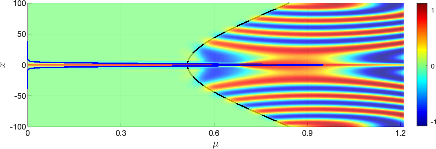
11 Conclusions and discussion

11.1 Conclusions

Considering the prototypical CGL PDE (1.1) as an equation in its own right, this article has presented a study of the phenomenon of delayed Hopf bifurcation (DHB) as the parameter $\mu$ increases slowly in time through an instantaneous Hopf bifurcation at $\mu=0$ . It has been shown that solutions with initial data given at $\mu_{0}\leq-\omega_{0}$ are not only near the attracting QSS while $\mu<0$ , but they remain near the QSS as $\mu$ continues to evolve slowly until well after it has become repelling and at least until $\mu$ reaches $\omega_{0}$ . This analysis of the delay of the Hopf bifurcation (DHB) was performed by directly using the classical methods of stationary phase and steepest descents on the linear PDE, based on the topography induced by the saddle point at $\mu=-i\omega_{0}$ , and followed by using an iterative method for solutions of the nonlinear PDE. Specifically, the nonlinear analysis is based on an iterative method for the difference between the solution $A$ of the full cubic PDE and the particular solution $A_{p}$ of the linear PDE.

Then, with these explicit results, it was shown that there is a competition at the heart of DHB between two exponentially small terms, one each from the particular solution $A_{p}(x,\mu)$ and the homogeneous solution $A_{h}(x,\mu)$ , to see which component first ceases to be exponentially small. The former stops being exponentially small and attains magnitude one along the space-time buffer curve, $\mu_{\rm stbc}(x)$ , and the latter along the homogeneous exit time curve, $\mu_{h}(x)$ . Explicit asymptotic formulas were derived, and their properties were illustrated with different types of source terms and initial data, including uni-modal, smoothed step function, and spatially periodic. Furthermore, in some of the examples, it is possible to calculate the curves from closed form solutions.

Based on an analysis of different outcomes of the competition between $\mu_{\rm stbc}(x)$ and $\mu_{h}(x)$ , i.e., between which comes first, several primary cases of DHB were introduced and analyzed. The first threes cases of DHB are for solutions $A(x,\mu)$ of (1.1) with initial data given at $\mu_{0}\leq-\omega_{0}$ . Here, Case 1 of DHB arises when the duration of the bifurcation delay is determined at all points by $\mu_{\rm stbc}(x)$ , i.e., when $\mu_{\rm stbc}(x)<\mu_{h}(x)$ for all $x$ . Case 2 of DHB occurs when the bifurcation delay is determined at some points by $\mu_{\rm stbc}(x)$ and at others by $\mu_{h}(x)$ . Case 3 of DHB arises when the duration of the delay is determined at all points by $\mu_{h}(x)$ , i.e., when $\mu_{h}(x)<\mu_{\rm stbc}(x)$ for all $x$ . Finally, Case 4 of DHB was introduced for solutions of (1.1) with initial data given at $-\omega_{0}<\mu_{0}<-\delta$ , where $\delta>0$ is small but $\mathcal{O}(1)$ . It was shown that, also for these solutions, the exit time from a neighbourhood of the repelling QSS can be spatially-dependent, as well.

Examples were presented of the different cases of DHB, and it was shown how to classify the DHB for general source terms $I_{a}(x)$ and various initial data. The local maxima of the source term and the initial data mark the sites at which the solution of the full cubic PDE (1.1) first diverges from the repelling QSS, and where the large-amplitude, post-DHB oscillations first set in. The spatial dependence of the DHB and onset of oscillations was shown to be quadratic in the case of Gaussians (uni-modal functions), a smoothed step function in the case of source terms given by an error function, and spatially-periodic in the case of spatially-periodic functions.

Finally, extensions of the main results were presented. Going beyond the main DHB results established for bounded and positive source terms, it was shown that DHB also occurs in the base case of (1.1) with algebraically-growing and sign-changing source terms. The formulas for the space-time buffer and homogeneous exit time curves (calculated either asymptotically or exactly) also accurately predict when the oscillations set in at each point $x$ , even though the source terms are not bounded or positive. Next, for the PDE with asymptotically large source terms ( $\beta=-\frac{1}{2}$ ), it was shown that the instantaneous Hopf bifurcation curve $\mu_{\rm Hopf}(x)$ can become large, even asymptotically large, so that the duration of the DHB can be asymptotically long. Combined with the information derived above about how the properties of the source terms determine the space-time buffer curve, this provides a high level of control or ability to design the spatial dependence of when the oscillations set in. Moreover, with large-amplitude source terms, it was found that there is more than one saddle point in the complex $\mu$ plane, and hence the topography of the Stokes and anti-Stokes lines is richer. A final extension concerns the case of $\mathcal{O}(1)$ diffusivity, for which the space-time buffer curve is also derived and found to be spatially flatter. That the method also extends to $\mathcal{O}(1)$ diffusivity enables application to a broader range of problems, in which the diffusivities are not necessarily small.

There are important considerations about the stability of the numerical simulations. As we have demonstrated throughout the article, the solutions are rapidly oscillating with frequency on the order of $\frac{\mu\omega_{0}}{\eps}$ . The numerical stiffness induced by the combination of rapid oscillations and slow drift in $\mu$ places an upper bound on the values of $\omega_{0}$ that can be used to reliably compute the solution near the repelling QSS. On the other hand, our space-time buffer curve predictions require that the leading order estimate of the spatially-dependent Hopf bifurcation, $\mu_{\rm Hopf}(x)=\frac{2\eps I_{a}(x)}{\omega_{0}^{2}}$ , is small. As such, the numerical values of $\omega_{0}$ that can be used are bounded from below, for any fixed value of $\eps$ . Thus, to address the stiffness and satisfy the smallness of $\mu_{\rm Hopf}(x)$ , we have chosen $\omega_{0}$ values in the range $C\eps^{1/4}<\omega_{0}<1$ , where $C$ is an $\mathcal{O}(1)$ constant. Many of our reported simulations use $0.5\leq\omega_{0}\leq 0.75$ for $\eps=0.01$ .

11.2 Post-DHB spatio-temporal patterns

Post DHB, several types of spatio-temporal patterns are observed depending on the type of inhomogeneity, the specific case of DHB, and the dispersion parameters $\alpha$ and $d_{I}$ . For instance, in Case 1 of DHB, Gaussian source terms break the $x$ -translation symmetry in the system, and we find that it leads to the bifurcation of large-amplitude periodic wave-trains which organize into stationary, or “pinned,” defects, see Figures 5 and 22.

In the nonlinear CGL (1.1), with the parameter $\mu>0$ held constant (i.e., $\mu_{t}=0$ ), periodic waves have the explicit form $re^{i(kx-\omega t)}$ with amplitude and nonlinear dispersion relations

r^{2}=\mu-\eps d_{R}k^{2},\qquad\qquad\omega(k)=-\omega_{0}+\alpha\mu-\eps(\alpha d_{R}-d_{I})k^{2}.

(11.1)

The amplitude relation shows that periodic patterns exist for wavenumbers $|k|<\sqrt{\mu/\eps d_{R}}$ . The dispersion relation shows that the frequency changes sign at $\mu=\frac{\omega_{0}}{\alpha}$ , provided $\alpha\neq 0$ , to leading order (with $0<\eps\ll 1$ and $k=\mathcal{O}(1)$ ). From these relations, the phase and group velocities for patterns with wavenumber $k$ take the form

c_{p}:=\omega(k)/k,\qquad\qquad c_{g}:=\omega^{\prime}(k) =2\eps(d_{I}-\alpha d_{R})k.

Then, for a dynamic Hopf parameter, we expect amplitudes to vary adiabatically as $\mu$ is increased, unless a stability boundary is reached, after which we expect a secondary dynamic bifurcation.

In Figure 5 (where $\alpha=0$ , $d_{R}=3,$ and $d_{I}=1$ ), we observe that the heterogeneity induces a symmetric defect which connects wavetrains of wavenumber $k_{+}=k$ and $k_{-}=-k$ on $x>0$ and $x<0$ , respectively, with $k\approx 1.15$ . Inward pointing phase curves indicate the arrangement $c_{p,-}>0>c_{p,+}$ which, since $\omega(k)<0$ for all $\mu$ and $\eps\ll 1$ , indicates a wavenumber arrangement $k_{-}<0<k_{+}$ . This then implies that the group velocities take the form $c_{g,-}<0<c_{g,+}$ , so that the defect is a source.

To leading order, a fixed wavenumber is selected at the space-time buffer curve which persists for increasing $\mu\in[0.5,2]$ with fixed oscillation frequency $\omega(k)$ (note that, with $\alpha=0$ , the frequency $\omega(k)$ has no direct dependence on $\mu$ ) and increasing amplitude $r(k)$ as $\mu$ increases. As the space time buffer curve expands in $x$ , additional periods of the wavetrains are added, leading to a persistent defect solution. We also remark that in Case 1, where the DHB is governed by the growth of the particular solution, the large amplitude pattern is independent of small white noise perturbations of the initial data. This indicates that such dynamic Hopf heterogeneities could be used in applications to select organised patterns.

In Figure 22 (where $\alpha>0$ , $d_{R}=1,d_{I}=0$ ), the defect dynamics are somewhat different. Both for $\alpha=0.1$ and $\alpha=0.6$ (see the top frames), the defect at $x=0$ is a symmetric sink. This may be seen as follows. For $\alpha=0.1$ , we find that $\omega(k)<0$ for $\mu\in[\mu_{\mathrm{stbc}}(x),\frac{\omega_{0}}{\alpha}]$ (which lies beyond the edge of the figure), and the phase velocities point inward. Hence, one readily calculates that, in this case, $c_{g,-}>0>c_{g,+}$ , so that the defect is a symmetric sink. Then, for $\alpha=0.6$ , a sink defect is also formed as $\mu$ increases past $\mu_{\mathrm{stbc}}(x)$ for $x\sim 0$ . As $\mu$ increases further, the frequency $\omega(k)$ changes sign at $\mu\approx\frac{\omega_{0}}{\alpha}=\frac{5}{6}$ to leading order in $\eps\ll 1$ so that phase velocities switch direction, $c_{p,-}<0<c_{p,+}$ . However, the defect is still a sink with inward pointing group velocities $c_{g,-}>0>c_{g,+}$ .

We remark that symmetric sink defects are in general transverse heteroclinic orbits when viewed in the appropriate spatial dynamics formulation, and come in one-parameter families parameterised by the wavenumber $k$ [57, 64]. Hence, we expect them to persist under the slow drift of $\mu$ . We also mention that source defects, which select the asymptotic wavenumbers $(k_{-},k_{+})$ , are not transverse heteroclinics and only exist for isolated asymptotic wavenumber pairs. These solutions are in general robust under the introduction of a small localised heterogeneity, and it is believed that they become pinned at the site of the heterogeneity, as we numerically observe here. It thus would be interesting to more fully understand how source and sink defects are selected in the presence of a spatio-temporal dynamic Hopf bifurcation.

For $\alpha$ yet larger, say $\alpha=2.5$ and $\alpha=5$ , we find that core and wave-train instabilities begin to arise. Since $d_{I}=0$ , the Benjamin-Feir condition $1+\alpha d_{I}>0$ holds and the band of stable wavenumbers is given, for stationary $\mu$ , by

|k|^{2}<\frac{\mu(1+\alpha d_{I})}{3+\alpha d_{I}+2\alpha^{2}}=\frac{\mu}{3+2\alpha^{2}}.

Hence, an increase in $\alpha$ brings a decrease in the range of stable wavenumbers. See [1, 64] for more information on this topic. The effects of adiabatic changes in $\mu$ on these large-amplitude spatio-temporal patterns is a topic of future research.

11.3 Open questions

The analysis and numerical simulations presented in this article raise a number of open questions and suggest avenues of additional research, beyond that on the effect of adiabatic variation in $\mu$ on the post-DHB spatio-temporal patterns, just discussed in Section 11.2.

The formal calculations in Sections 2 and 6 of the attracting and repelling QSS of the linear and nonlinear systems for $\mu<0$ and $\mu>0$ , respectively, show that they are unique to all orders, but differ in the exponentially small terms. This suggests studying the Gevrey regularity properties of the QSS. Moreover, this question is motivated directly by the recent demonstration that slow manifolds for analytic fast-slow systems of ODEs are Gevrey regular, in the absence of singularities in the slow flow, see [17], which is a major extension of the classical results in [24].

Next, we expect that the nonlinear analysis of Section 6, which is only formal in this article, could be made rigorous and used to prove the convergence of the sequence of functions $\{b_{j}\}$ in an appropriate function space. In particular, one would try to show that

e^{\frac{1}{2\eps}(\mu+i\omega)^{2}}(b_{j+1}-b_{j})\sim \eps^{\frac{2j+3}{2}},

uniformly in $x$ to conclude that $\{b_{j}\}_{j\in\mathbb{N}}$ is Cauchy and hence convergent to a fixed point $b_{*}$ of the mapping $H$ as $j\rightarrow+\infty$ . This limiting fixed point would, by construction, yield a solution of the mild formulation (6.5) with the desired dynamics for $\mu\in[\mu_{0},\omega_{0}-\tilde{\delta})$ . Standard bootstrapping and energy estimate methods [42] could be used to lift this mild solution to a classical solution.

The results in the base case of (1.1) with unbounded and sign-changing source terms (Section 8) raise the question about how to generalize the analysis of DHB beyond the assumptions made here. Good agreement is found between the analytically calculated DHB and numerically calculated exit times from the neighbourhood of the repelling QSS and the onset of the oscillations, even though the general conditions in Section 2 are not satisfied with these source terms.

In the study of DHB for solutions of (1.1), the analyses of $A_{h}$ , the homogeneous component, in Section 4 and of the solution $A$ of the full cubic PDE (1.1) in Section 6 were done working with $\mu$ on the real line. Analyticity was used in the study of the particular solution, $A_{p}$ , of the linear PDE, to deform the contour in the complex $\mu$ plane to derive the space-time buffer curve. It is of interest to determine whether analyticity is strictly necessary for DHB, or instead if some slightly weaker assumption might suffice to observe DHB. We refer to sections 2 and 3 of [4], for example, for aspects of the general theory of Gevrey regularity of dissipative PDEs with analytic nonlinearities. Also, there is a well-developed theory of Gevrey regularity for solutions of nonlinear R-D equations on bounded domains, see for example [53], especially the results for the GL equation in section 2.2 there. This could be useful for developing a better understanding of DHB in nonlinear R-D equations, the minimal hypotheses necessary for it, and the Gevrey regularity of the solutions.

There are a number of possible avenues to explore to rigorously determine whether or not slow invariant manifolds exist on $\mu\in[\mu,-\delta)$ and $\mu\in(-\delta,-\mu_{0}]$ , respectively. We are presently studying this question for (1.1) using scaling variables on the real line and previous results on slow manifolds; see for example [34] and references therein.

Finally, the type of competition analyzed herein between the homogeneous and particular solutions of the linearised problem, in terms of which stops being exponentially small first and transitions through modulus one to becoming exponentially large, arises in other PDEs. We are currently exploring it in a number of other reaction-diffusion systems that exhibit DHB, see [36].

Acknowledgements

We thank Antonella Cucchetti, Arjen Doelman, Edgar Knobloch, and Gene Wayne, for useful comments and questions. T.K. and T.V. thank the Lorentz Center (Leiden University, NL) for their hospitality and stimulating research environment during the 2017 Workshop on Singular Perturbation Theory. T.K. thanks the organisers of the February 2019 conference on Advances in Pattern Formation (Ben-Gurion University, Israel), where the initial results about DHB in the CGL equation were presented. T.K. is grateful to Prof. G.B. Whitham, from whom he learned the methods of stationary phase and steepest descents. This work was supported by the US National Science Foundation [DMS-2006887 to R.G., DMS-1616064 to T.J.K., and DMS-1853342 to T.V.].

References

[1] I.S. Aranson and L. Kramer [2002], The world of the Complex Ginzburg-Landau equation, Rev. Mod. Phys., 74, 99-143
[2] P. Ashwin, S. Wieczorek, R. Vitolo, and P. Cox [2012], Tipping points in open systems: Bifurcation, noise-induced and rate-dependent examples in the climate system, Phil. Trans. R. Soc. A, 370, 1166-–1184
[3] D. Avitabile, M. Desroches, R. Veltz, and M. Wechselberger [2020], Local theory for spatio-temporal canards and delayed bifurcations, SIAM J. Math. An., 52, 5703-5747
[4] H. Bae and A. Biswas [2015], Gevrey regularity for a class of dissipative equations with analytic nonlinearity, Meth. Applic. An., 22, 377-408
[5] S.M. Baer, T. Erneux, and J. Rinzel [1989], The slow passage through a Hopf bifurcation: delay, memory effects, and resonance, SIAM J. Appl. Math., 49, 55–71
[6] W. Balser [2005], Power series solutions of the inhomogeneous heat equation, Recent Trends in Microlocal Analysis, Kokyuroku RIMS, 1412, 151-159
[7] E. Barreto and J.R. Cressman [2011], Ion concentration dynamics as a mechanism for neuronal bursting, J. Biol. Phys. 37, 361-–373
[8] C.M. Bender and S.A. Orszag [1999], Advanced Mathematical Methods for Scientists and Engineers: Asymptotic Methods and Perturbation Theory, Springer-Verlag, New York
[9] F. Berthier, J.-P. Diard, and S. Nugues [1997], On the nature of the spontaneous oscillations observed for the Koper-Sluyters electrocatalytic reaction, J. Electroanalytical Chem., 436, 35–42
[10] R. Bertram, M. Butte, T. Kiemel, and A. Sherman [1995], Topological and phenomenological classification of bursting oscillations, Bull. Math. Biol., 57, 413–-439
[11] L.M. Bilinsky and S. M. Baer [2018], Slow passage through a Hopf bifurcation in excitable nerve cables: Spatial delays and spatial memory effects, Bull. Math. Bio., 80, 130-–150
[12] C. Borgers, M. Krupa, and S. Gielen [2010], The response of a classical Hodgkin-Huxley neuron to an inhibitory input pulse, J. Comp. Neurosci., 28, 509–526.
[13] B. Braaksma [1993], Critical phenomena in dynamical systems of van der Pol type, Ph.D. Thesis, Utrecht University, NL
[14] S.J. Chapman, J.R. King, and K.L. Adams [1998], Exponential asymptotics and Stokes lines in nonlinear ordinary differential equations, Proc. Roy. Soc. Lond. A, 454, 2733-2755
[15] S.J. Chapman and D.B. Mortimer [20015], Exponential asymptotics and Stokes lines in partial differential equations, Proc. Roy. Soc. Lond. A, 461, 2385-2421
[16] C.A. Del Negro, C.-F. Hsiao, S.H. Chandler, and A. Garfinkel [1998], Evidence for a novel bursting mechanism in rodent trigeminal neurons, Biophys. J., 75, 174-–182
[17] P. De Maesschalck and K. Kenens [2020], Gevrey properties of slow manifolds, Nonlinearity, 33, 341-387
[18] R.B. Dingle [1973], Asymptotic expansions: Their derivation and interpretation, Academic Press, London, UK
[19] M. Dolnik, I. Berenstein, A.M. Zhabotinsky, and I.R. Epstein [2001], Spatial periodic forcing of Turing structures, Phys. Rev. Lett., 87, 238301
[20] W. Eckhaus [1983], Relaxation oscillations including a standard chase on French ducks, in Asymptotic Analysis II, F. Verhulst (ed.) LNM, 985, Springer, Berlin, 449-494
[21] H. Engler, H.G. Kaper, T.J. Kaper, and T. Vo [2017], Dynamical systems analysis of the Maasch-Saltzman model for glacial cycles, Physica D, 359, 1-–20
[22] T. Erneux and E. Reiss [1990], Delaying the Transition to Hopf Bifurcation by Slowly Varying the Bifurcation Parameter,” in Spatial inhomogeneities and transient behaviour in chemical kinetics, P. Gray, G. Nicolis, F. Baras, P. Borckmans, and S. Scott, eds., Proc. Nonlin. Sci., Manchester University Press, Manchester, Chap. 18, 267–-278
[23] T. Erneux, E. Reiss, L. Holden, and M. Georgiou [1991], Slow passage through bifurcations and limit points: Asymptotic theory and applications, in Dynamic Bifurcations, Lecture Notes in Math., 1493, E. Benoit, ed., Springer, Berlin, 14–-28
[24] N. Fenichel [1979], Geometric singular perturbation theory for ordinary differential equations, J. Diff. Eq., 31, 53–98
[25] D. Golomb, K. Donner, L. Shachan, D. Shlosberg, Y. Amitai, and D. Hansel, Mechanisms of firing patterns in fast-spiking cortical interneurons, PLOS Comp. Bio., 3, e156
[26] M. Golubitsky, K. Josic, and T.J. Kaper [2001], An unfolding theory approach to bursting in fast-slow systems, in Global Analysis of Dynamical Systems, H.W. Broer, B. Krauskopf, and G. Vegter (eds.), Institute of Physics, Bristol, UK, 277–308
[27] J. Grasman and J.J. Wentzel [1994], Co-existence of a limit cycle and an equilibrium in Kaldor’s business cycle model and its consequences, J. Econ. Behav. Organization, 24, 369–377
[28] L. Haim, A. Hagbereg, and E. Meron [2015], Non-monotonic resonance in a spatially-forced Lengyel-Epstein model, Chaos, 25, 064307
[29] X. Han, F. Xia, P. Ji, Q. Bi, and J. Kurths [2016], Hopf-bifurcation-delay-induced bursting patterns in a modified circuit system, Comm. Nonlin. Sci. Num. Sim., 36, 517–527
[30] M. Haragus and G. Iooss [2010], Local Bifurcations, Center Manifolds, and Normal Forms in Infinite-Dimensional Dynamical Systems, Springer, London
[31] M.G. Hayes, T.J. Kaper, P. Szmolyan, and M. Wechselberger [2016], Geometric desingularization of degenerate singularities in the presence of fast rotation: A new proof of known results for slow passage through Hopf bifurcations, Indag. Math., $\bf 27$ , 1184–1203
[32] M. Higuera, J. Porter, and E. Knobloch [2008], Faraday waves, streaming flow, and relaxation oscillations in nearly circular containers, Chaos, 18, 015104
[33] L. Holden and T. Erneux [1993], Slow passage through a Hopf bifurcation: From oscillatory to steady state solutions, SIAM J. Appl. Math., 53, 1045-–1058
[34] F. Hummel and C. Kuehn [2020], Slow manifolds for infinite-dimensional evolution equations, preprint, arxiv:2008.10700
[35] E. Izhikevich [2001], Synchronization of elliptic bursters, SIAM Rev., 43, 315-–344
[36] T.J. Kaper and T. Vo [2018], Delayed loss of stability due to the slow passage through Hopf bifurcations in reaction-diffusion equations, Chaos, $\bf 28$ , 091103
[37] J. Kevorkian and J.D. Cole [1981], Perturbation Methods in Applied Mathematics, Applied Mathematical Sciences series, vol. 34, Springer, New York
[38] M.T.M. Koper and B.D. Aguda [1996], Experimental demonstration of delay and memory effects in the bifurcations of nickel electrodissolution, Phys. Rev. E, 54, 960–963
[39] M.T.M. Koper [1998], Non-linear phenomena in electrochemical systems, J. Chem. Soc. Faraday Trans., 94, 1369–-1378
[40] P. Kügler [2016], Early Afterdepolarizations with growing amplitudes via delayed sub-critical Hopf bifurcations and unstable manifolds of saddle-foci in cardiac action potential dynamics, PLOS One, 11, e0151178
[41] C. Kuehn [2015], Multiple Time Scale Dynamics, Applied Mathematical Sciences series, vol. 191, Springer, New York
[42] C.D. Levermore and M. Oliver [1996]. The complex Ginzburg-Landau equation as a model problem, Lectures in Applied Mathematics 3. 141-190, AMS, Providence, Rhode Island.
[43] D.A. Lutz, M. Miyake, and R. Schäfke [1999], On the Borel summability of divergent solutions of the heat equation, Nagoya Math. J., 154, 1-29
[44] K.A. Maasch and B. Saltzman [1990], A low-order dynamic model of global climate variability over the full Pleistocene, J. Geophys. Res., 95, D2:1955–1963
[45] P.D. Miller [2006], Applied Asymptotic Analysis, AMS Graduate Studies in Applied Mathematics, 75, Providence
[46] J.D. Murray [1984], Asymptotic Analysis, 2nd ed. Applied Mathematical Sciences series, vol. 48, Springer, New York
[47] A.I. Neishtadt [1987], Persistence of stability loss for dynamical bifurcations. I, Diff. Urav., 23, 2060–2067 (Russian). [English translation: Diff. Eq., 23 (1988) 1385–1391, Plenum Pub. Corp.]
[48] A.I. Neishtadt [1988], Persistence of stability loss for dynamical bifurcations. II, Diff. Urav., 24, 226–233 (Russian). [English translation: Diff. Eq., 24 (1988) 171–176, Plenum Pub. Corp.]
[49] E.W. Ng and M. Geller [1969], A table of integrals of the error functions, J. Res. Nat. Bur. Standards – B. Mathematical Sciences, 73B (1), 1–20
[50] F.W.J. Olver [1974], Asymptotics and special functions, AK Peters, Wellesley, MA.
[51] Y. Park, Y. Do, and J.M. Lopez [2011], Slow passage through resonance, Phys. Rev. E, 84, 056604
[52] D. Premraj, K. Suresh, T. Banerjee, and K. Thamilmaran [2016], An experimental study of slow passage through Hopf and pitchfork bifurcations in a parametrically-driven nonlinear oscillator, Comm. Nonlin. Sci. Num. Sim., 37, 212-221
[53] K. Promislow [1991], Time analyticity and Gevrey regularity for solutions of a class of dissipative partial differential equations, Nonlin. An., Theory, Meth., Applic., 16, 959-980
[54] P. Remy [2019], Gevrey index theorem for the inhomogeneous $n$ -dimensional heat equation with a power-law nonlinearity and variable coefficients, HAL archives-ouvertes, hal-02117418, preprint.
[55] J. Rinzel and S. Baer [1988], Firing threshold of the Hodgkin-Huxley model for a slow current ramp: A memory effect and its dependence on fluctuations, Biophys. J., 54, 551–-555
[56] J. Rubin and D. Terman [2002], Geometric singular perturbation analysis of neuronal dynamics, in Handbook of Dynamical Systems, volume 2, B. Fiedler, ed., Elsevier, chapter 3, 93-–146
[57] B. Sandstede and A. Scheel [2004], Defects in oscillatory media: toward a classification, SIAM Journal on Applied Dynamical Systems 3, 1-68
[58] M.A. Shishkova [1973], A discussion of a certain system of differential equations with a small parameter multiplying the highest derivatives, Dokl. Akad. Nauk SSSR, 209, 576–579
[59] P. Shorten and D. Wall [2000], A Hodgkin-Huxley model exhibiting bursting oscillations, Bull. Math. Biol., 62, 695-–715
[60] R. Speth, W. Green, S. MacNamara, and G. Strang [2013], Balanced splitting and rebalanced splitting, SIAM J. Numer. Anal., 51, 3084-3105
[61] P. Strizhak and M. Menzinger [1996], Slow passage through a supercritical Hopf bifurcation: Time-delayed response in the Belousov-Zhabotinsky reaction in a batch reactor, J. Chem. Phys., 105, 10905
[62] J. Su [1993], Delayed oscillation phenomena in the FitzHugh Nagumo equation, J. Diff. Eq., 105, 180–215
[63] G. Ullah, Y. Wei, M.A. Dahlem, M. Wechselberger, and S.J. Schiff [2015], The role of cell volume in the dynamics of seizure, spreading depression, and anoxic depolarization, PLOS Comp. Bio., 11, e1004414
[64] W. van Saarloos [1992], Fronts, pulses, sources and sinks in generalized complex Ginzburg-Landau equations, Physica D, 56, 302-367
[65] T. Vo, R. Bertram, and T.J. Kaper [2020], Multi-mode attractors and spatio-temporal canards, Physica D, 411, 132544
[66] M. Wechselberger [2020], Geometric Singular Perturbation Theory Beyond the Standard Form, Frontiers in Applied Dynamical Systems: Reviews and Tutorials, 6, Springer, New York
[67] H. Wu, Y. Ye, M. Chen, A. Xu, and B. Bao [2019], Extremely slow passages in a low-pass filter-based memristive oscillator, Nonlinear Dynamics, 97, 2339–2353

Appendix A Second parametrisation for the integral $\mathcal{I}_{a2}$ in Section 2.2

In this appendix, we briefly show that $\mathcal{I}_{a2}$ (2.13) may be derived also using a second, implicit parametrisation (by $\sigma$ ) of the contour $C_{a2}$ ,

C_{a2}:\quad-\frac{1}{2}({\tilde{\mu}}+i\omega_{0})^{2}=-\frac{1}{2}(\mu+i\omega_{0})^{2}+\sigma,\quad\sigma\leq 0.

(A.1)

Here, $\sigma$ increases monotonically along $C_{a2}$ , starting from $-\infty$ , hitting $-\frac{1}{2}(\omega_{0}^{2}-\mu^{2})$ at $q_{a}$ , and continuing up to zero at the point $\mu$ . Therefore, the integral for $\mathcal{I}_{a2}$ may be written as

\mathcal{I}_{a2}=\frac{e^{-\frac{1}{2\eps}(\mu+i\omega_{0})^{2}}}{\sqrt{\eps}}\int_{-\infty}^{0}g(x,\mu-{\tilde{\mu}}(\sigma))e^{\frac{\sigma}{\eps}}\frac{d{\tilde{\mu}}}{d\sigma}d\sigma.

(A.2)

Now, we fix $\Delta>0$ sufficiently small, independent of $\eps$ . The dominant contribution to the integral comes from $\sigma\in(-\Delta,0]$ , since the integrand in $\mathcal{I}_{a2}$ is exponentially small for all $\sigma<-\Delta$ , due to the exponential term, where we recall $\mu\in[-\omega_{0},-\delta]$ is fixed, $g$ is analytic and hence bounded, and the differential is bounded along $C_{a2}$ . Taylor expanding $g$ and the differential about $\sigma=0$ , and using ${\tilde{\mu}}(\sigma)=-i\omega_{0}+(\mu+i\omega_{0})\left[1-\frac{2\sigma}{(\mu+i\omega_{0})^{2}}\right]^{\frac{1}{2}},$ we find

g(x,\mu-{\tilde{\mu}}(\sigma))=g\left(x,\mu+i\omega_{0}-(\mu+i\omega_{0})\left[1-\frac{2\sigma}{(\mu+i\omega_{0})^{2}}\right]^{\frac{1}{2}}\right)=g\left(x,\frac{\sigma}{\mu+i\omega_{0}}+\mathcal{O}\left(\frac{\sigma^{2}}{(\mu+i\omega_{0})^{3}}\right)\right),

(A.3)

\frac{d{\tilde{\mu}}}{d\sigma}=\frac{-1}{(\mu+i\omega_{0})}\left[1-\frac{2\sigma}{(\mu+i\omega_{0})^{2}}\right]^{-\frac{1}{2}}=\frac{-1}{(\mu+i\omega_{0})}\left[1+\frac{\sigma}{(\mu+i\omega_{0})^{2}}+\mathcal{O}\left(\frac{\sigma^{2}}{(\mu+i\omega_{0})^{4}}\right)\right].

(A.4)

Hence,

\mathcal{I}_{a2}=\frac{-e^{-\frac{1}{2\eps}(\mu+i\omega_{0})^{2}}}{\sqrt{\eps}(\mu+i\omega_{0})}\int_{-\Delta}^{0}g\left(x,\frac{\sigma}{\mu+i\omega_{0}}+\mathcal{O}\left(\frac{\sigma^{2}}{(\mu+i\omega_{0})^{3}}\right)\right)e^{\frac{\sigma}{\eps}}\left[1+\mathcal{O}\left(\frac{\sigma}{(\mu+i\omega_{0})^{2}}\right)\right]d\sigma.

(A.5)

Then, by (2.6)(b) and standard properties of the 1-D heat kernel, we observe that $\lim_{\chi\to 0^{+}}g(x,\chi)=I_{a}(x).$ Therefore, we directly obtain (2.13), and hence the same formula for $A_{p}$ .

Remark. The two parametrisations (2.10) and (A.1) are consistent. For example, expressing (2.10) in terms of small $|\sigma|$ , we find ${\tilde{\mu}}_{R}(\sigma)=\mu-\frac{\mu\sigma}{\mu^{2}+\omega_{0}^{2}}+\mathcal{O}(\sigma^{2})$ , and hence ${\tilde{\mu}}(\sigma)=\mu-\frac{\mu-i\omega_{0}}{\mu^{2}+\omega_{0}^{2}}\sigma+\mathcal{O}(\sigma^{2})$ , via (2.10). This is identical to the expansion of (A.1), ${\tilde{\mu}}(\sigma)=\mu-\frac{\sigma}{(\mu+i\omega_{0})}+\mathcal{O}\left(\frac{\sigma^{2}}{(\mu+i\omega_{0})^{3}}\right).$

Appendix B The solutions of (2.1) are also near the QSS for $\mu\in(-\delta,\delta)$

In this appendix, we briefly show how the asymptotic analysis of the solutions $A_{p}(x,\mu)$ of the linear CGL (2.1) in the base case, which was carried out separately for $\mu\in[-\omega_{0},-\delta]$ in Section 2.2 and for $\mu\in[\delta,\omega_{0}]$ , in Section 2.3 extends to $\mu\in(0,\delta)$ , and to $\mu\in(-\delta,0]$ , where we recall that $\delta>0$ is $\mathcal{O}(1)$ and small.

First, we consider the case of $\mu\in(0,\delta)$ . The contour is again $C_{r}=C_{r1}\bigcup C_{r2}\bigcup C_{r3}\bigcup C_{r4}$ , as in the previous subsection. Here, the point $q_{r}$ is close to the saddle at $-i\omega_{0}$ since $\mu\in(0,\delta)$ , recall Figure 3. The contribution from $C_{r1}$ and $C_{r2}$ is again

A_{p}(x,\mu)=\sqrt{\frac{\pi}{2}}\left(g(x,\mu+i\omega_{0})+\mathcal{O}(\sqrt{\eps})\right)e^{\frac{1}{2\eps}(\mu+i\omega_{0})^{2}},

(B.1)

where the dominant contribution comes from the final portion of the rise along $C_{r2}$ , the steepest ascents path up to the saddle. Then, the contributions along $C_{r3}$ and $C_{r4}$ yield

\begin{split}A_{p}(x,\mu)&=-\sqrt{\eps}\frac{I_{a}(x)}{\mu+i\omega_{0}}+\eps^{\frac{3}{2}}\left(\frac{I_{a}(x)+d(\mu+i\omega_{0}){I_{a}}^{\prime\prime}(x)}{(\mu+i\omega_{0})^{3}}\right)+\mathcal{O}\left(\frac{\eps^{\frac{5}{2}}}{(\mu+i\omega_{0})^{5}}\right)\\ &+\left(\sqrt{\frac{\pi}{2}}+c(\mu)\right)\left(g(x,\mu+i\omega_{0})+\mathcal{O}(\sqrt{\eps})\right)e^{\frac{1}{2\eps}(\mu+i\omega_{0})^{2}}.\end{split}

(B.2)

Here, $c(\mu)=(1+i)\int_{0}^{\sqrt{\frac{\omega_{0}\mu}{\eps}}}e^{-i{\tilde{\sigma}}^{2}}d{\tilde{\sigma}}$ , which comes from the contribution along $C_{r3}$ , the stationary phase path from emerging from the saddle; recall (2.19). The function $c(\mu)$ increases monotonically from zero in the limit $\mu\to 0^{+}$ to $\sqrt{\frac{\pi}{2}}$ for $\delta>0$ and for other ${\cal O}(1)$ values of $\mu>0$ .

Next, we consider the case of $\mu\in(-\delta,0)$ . We again use the contour $C_{a}$ from Section 2.2, recall Figure 2. Then, $A_{p}(x,\mu)$ is given by (2.15), since also for $\mu\in(-\delta,0)$ the dominant part comes from the final segment up to $\mu$ on the real axis.

Finally, we consider the case of $\mu=0$ . The contour of integration is the union of the line segments

\mathcal{L}_{1}=\{{\tilde{\mu}}_{I}=-\omega_{0},{\tilde{\mu}}_{R}\leq 0\}\quad{\rm and}\quad\mathcal{L}_{2}=\{{\tilde{\mu}}_{R}=0,-\omega_{0}\leq{\tilde{\mu}}_{I}\leq 0\}.

(B.3)

These line segments lie on the horizontal and vertical anti-Stokes lines $\psi=0$ , respectively, through the saddle. Application of the method of steepest descents along $\mathcal{L}_{1}$ yields $\left(\sqrt{\frac{\pi}{2}}g(x,i\omega_{0})+\mathcal{O}(\sqrt{\eps})\right)e^{-\frac{\omega_{0}^{2}}{2\eps}}$ .

Then, the contribution from the steepest ascents path $\mathcal{L}_{2}$ consists of two pieces, one from the lower limit of integration and a second piece from the upper limit of integration at ${\tilde{\mu}}=0$ . The former cancels out the contribution from $\mathcal{L}_{1}$ . Hence, for $\mu=0$ , we find

A_{p}(x,0)=\sqrt{\eps}\frac{iI_{a}(x)}{\omega_{0}}+\eps^{\frac{3}{2}}\left(\frac{iI_{a}(x)-d\omega_{0}I_{a}^{\prime\prime}(x)}{\omega_{0}^{3}}\right)+\mathcal{O}(\eps^{\frac{5}{2}}).

(B.4)

Therefore, the solution is also the QSS to all orders at $\mu=0$ , just as for $\mu\in(-\delta,0)$ and for $\mu\in(0,\delta)$ .

$\displaystyle\Bigg\\|-\frac{1+i\alpha}{\eps}$	$\displaystyle\int_{\mu_{0}}^{\mu}E(\tilde{\mu})G_{d}(\mu-\tilde{\mu})*\left[\tilde{c}(\tilde{\mu})^{3}g(\cdot,\tilde{\mu}+i\omega_{0})\|g(\cdot,\tilde{\mu}+i\omega_{0})\|^{2}+\mathcal{O}(\eps^{1/2})\right]d\tilde{\mu}\Big\\|_{L^{\infty}}$
	$\displaystyle=\Bigg\\|-\frac{1+i\alpha}{\eps}\int_{-\delta}^{\mu}E(\tilde{\mu})G_{d}(\mu-\tilde{\mu})*\left[\tilde{c}(\tilde{\mu})^{3}g(\cdot,\tilde{\mu}+i\omega_{0})\|g(\cdot,\tilde{\mu}+i\omega_{0})\|^{2}+\mathcal{O}(\eps^{1/2})\right]d\tilde{\mu}\Bigg\\|$
	$\displaystyle\leq\|1+i\alpha\|\eps^{-1}E(\mu)\tilde{c}(\mu)^{3}\int_{-\delta}^{\mu}\\|G_{d}(\mu-\tilde{\mu})*\left[g(\cdot,\tilde{\mu}+i\omega_{0})\|g(\cdot,\tilde{\mu}+i\omega_{0})\|^{2}+\mathcal{O}(\eps^{1/2})\right]\\|_{L^{\infty}}d\tilde{\mu}$
	$\displaystyle\leq CE(\mu)(\eps^{-1}+\mathcal{O}(1))\\|I_{a}\\|_{L^{\infty}}^{3}$	(6.11)

$\displaystyle\Bigg\\|-\frac{1+i\alpha}{\eps}$	$\displaystyle\int_{\mu_{0}}^{\mu}E(\tilde{\mu})G_{d}(\mu-\tilde{\mu})*\left[2B_{p,2}\|B_{p,1}\|^{2}\right]d\tilde{\mu}\Big\\|_{L^{\infty}}$
	$\displaystyle=2\Bigg\\|-\frac{1+i\alpha}{\eps}\int_{-\delta}^{\mu}G_{d}(\mu-\tilde{\mu})*\left[(\tilde{c}(\tilde{\mu})g(\cdot,\tilde{\mu}+i\omega_{0})+\mathcal{O}(\eps^{1/2}))\cdot\left\|\frac{\eps^{1/2}I_{a}}{\tilde{\mu}+i\omega_{0}}+\mathcal{O}(\eps^{3/2})\right\|^{2}\right]d\tilde{\mu}\Bigg\\|_{L^{\infty}}$
	$\displaystyle\leq 2\|1+i\alpha\|\tilde{c}(\mu)\int_{-\delta}^{\mu}\Big\\|G_{d}(\mu-\tilde{\mu})*\left[g(\cdot,\tilde{\mu}+i\omega_{0})\cdot\left\|\frac{I_{a}}{\tilde{\mu}+i\omega_{0}}\right\|^{2}+\mathcal{O}(\eps)\right]\Big\\|_{L^{\infty}}d\tilde{\mu}$
	$\displaystyle\leq C\\|I_{a}\\|_{L^{\infty}}^{3}+\mathcal{O}(\eps).$	(6.12)

Delayed Hopf bifurcation and space-time buffer curves in the Complex Ginzburg-Landau equation

Abstract

1 Introduction

2 Linear analysis for solutions with μ0<−ω0\mu_{0}<-\omega_{0}

2.1 The homogeneous and particular solutions

2.2 Tracking the particular solutions near the attracting QSS

2.3 Tracking the particular solutions near the repelling QSS

3 The space-time buffer curve

3.1 Derivation of the space-time buffer curve, μstbc​(x)\mu_{\rm stbc}(x)

3.2 Examples of the space-time buffer curve, μstbc​(x)\mu_{\rm stbc}(x)

4 The homogeneous exit time curve, μh​(x)\mu_{h}(x)

5 The main cases of DHB: one case for each different type of outcome in the competition between which of ApA_{p} and AhA_{h} ceases to be exponentially small first

5.1 Cases 1-3 of DHB for solutions with initial data given at μ0≤−ω0\mu_{0}\leq-\omega_{0}

5.2 Case 4 of DHB for initial data given at any −ω0<μ0≤−δ-\omega_{0}<\mu_{0}\leq-\delta

6 DHB and the space-time buffer curve for the cubic CGL

6.1 Iterative framework and base iterate

6.2 Inductive step

7 The 𝒪⁡(ε)\mathcal{O}(\eps) value of μHopf​(x)\mu_{\rm Hopf}(x) in the base case

8 Spatially growing and sign-changing source terms

8.1 An algebraically-growing source term

8.2 A sign-changing source term

9 Asymptotically large source terms

10 An example with 𝒪⁡(1)\mathcal{O}(1) diffusivity and 𝒪⁡(1)\mathcal{O}(1) source term

10.1 The 𝒪⁡(1)\mathcal{O}(1) QSS and μHopf​(x)\mu_{\rm Hopf}(x) for (10.1)

10.2 The space-time buffer curve for the linearised version of (10.1)

11 Conclusions and discussion

11.1 Conclusions

11.2 Post-DHB spatio-temporal patterns

11.3 Open questions

Acknowledgements

References

Appendix A Second parametrisation for the integral ℐa​2\mathcal{I}_{a2} in Section 2.2

Appendix B The solutions of (2.1) are also near the QSS for μ∈(−δ,δ)\mu\in(-\delta,\delta)

2 Linear analysis for solutions with $\mu_{0}<-\omega_{0}$

3.1 Derivation of the space-time buffer curve, $\mu_{\rm stbc}(x)$

3.2 Examples of the space-time buffer curve, $\mu_{\rm stbc}(x)$

4 The homogeneous exit time curve, $\mu_{h}(x)$

5 The main cases of DHB: one case for each different type of outcome in the competition between which of $A_{p}$ and $A_{h}$ ceases to be exponentially small first

5.1 Cases 1-3 of DHB for solutions with initial data given at $\mu_{0}\leq-\omega_{0}$

5.2 Case 4 of DHB for initial data given at any $-\omega_{0}<\mu_{0}\leq-\delta$

7 The $\mathcal{O}(\eps)$ value of $\mu_{\rm Hopf}(x)$ in the base case

10 An example with $\mathcal{O}(1)$ diffusivity and $\mathcal{O}(1)$ source term

10.1 The $\mathcal{O}(1)$ QSS and $\mu_{\rm Hopf}(x)$ for (10.1)

Appendix A Second parametrisation for the integral $\mathcal{I}_{a2}$ in Section 2.2

Appendix B The solutions of (2.1) are also near the QSS for $\mu\in(-\delta,\delta)$