Gradient-based optimization of 3D MHD equilibria

The equilibrium code may return with an error for a given plasma boundary. There are many reasons for these failures, such as the flux coordinate Jacobian becoming ill-conditioned or the number of iterations exceeding the maximum prescribed value. When such a failure is experienced during the optimization, the objective function is set to an arbitrarily large value (e.g., $10^{12}$) to enforce an effective constraint. The approach of assigning a very large fictitious objective value at unevaluable points is common in the optimization literature (Rasheed et al. 1997; Emmerich et al. 2002) and is employed in the STELLOPT code (Lazerson et al. 2020).

As encountering such unevaluable points makes the parameter space non-smooth, it is prudent to try to avoid code failures by placing additional constraints on the parameter space. Such a technique has been employed in the optimization of aircraft by checking that simulation outputs match physical model assumptions, such as the drag coefficient being non-negative (Gelsey 1995; Gelsey et al. 1998). In §3, we present constraints which prevent the surface from self-intersecting or from obtaining large curvature, leading to an ill-conditioned Jacobian and code failure. Even in the presence of such constraints, unevaluable points may still be present. Here the objective function becomes discontinuous, which is problematic for optimizers which assume function continuity. In this work we employ the BFGS quasi-Newton method with an Armijo-Wolfe line search, which assumes $C^{2}$ continuity of the objective function (Nocedal & Wright 2006). Although convergence of the BFGS algorith is not guaranteed for non-smooth problems, it has been observed that a reasonable approximation to the optimum is most often achieved (Lemaréchal 1982). With the standard Armijo-Wolfe line search method, the gradient need not be evaluated unless the objective function satisfies the sufficient decrease criterion. Thus the gradient does not need to be evaluated at unevaluable points. In this way, as long as the line search never returns a point where the objective is not differentiable, the BFGS method is well defined. While there are specialized quasi-Newton methods for non-smooth objective functions (Lewis & Overton 2009), we have obtained acceptable results with a standard BFGS method.

We now describe a constraint which prevents self-intersection of the plasma boundary. Given a surface described by the cylindrical coordinates $R(\theta,\phi)$ and $Z(\theta,\phi)$, self-intersection of the boundary may occur if either:

		(a) $R(\theta,\phi)<0$ at any point, or
		(b) the planar curve $\textbf{x}_{\phi_{0}}(\theta)=\{R(\theta,\phi_{0}),Z(\theta,\phi_{0})\}$ is self-intersecting for any $\phi_{0}$.

Condition (a) can be avoided using a penalty objective of the form,

$\displaystyle f_{R}(S_{P})=\frac{1}{A_{P}}\int_{S_{P}}d^{2}x\,\exp\left(-\frac{\left(R-R_{\text{min}}\right)}{w_{R}}\right),$

(8)

where $w_{R}$ is a weight which sets the gradient length scale of the objective, $R_{\text{min}}$ is the minimum allowable major radius, and $A_{P}$ is the area of $S_{P}$.

Condition (b) can be avoided by introducing a constraint on the global radius of curvature (Gonzalez & Maddocks 1999; Walker 2016) of each of the curves, $\textbf{x}_{\phi_{0}}(\theta)$, which will now be defined. The radius of the unique circumcircle containing any three points $\textbf{x}_{1}$, $\textbf{x}_{2}$, and $\textbf{x}_{3}$ (Figure 1), can be computed from,

$\displaystyle\rho(\textbf{x}_{1},\textbf{x}_{2},\textbf{x}_{3})=\frac{|\textbf{x}_{1}-\textbf{x}_{2}||\textbf{x}_{1}-\textbf{x}_{3}||\textbf{x}_{2}-\textbf{x}_{3}|}{4\mathcal{A}(\textbf{x}_{1},\textbf{x}_{2},\textbf{x}_{3})},$

(9)

where $\mathcal{A}(\textbf{x}_{1},\textbf{x}_{2},\textbf{x}_{3})$ is the area of a triangle with vertices $\textbf{x}_{1}$, $\textbf{x}_{2}$, and $\textbf{x}_{3}$. Under the assumption that these points lie on a non-self-intersecting smooth curve, $\mathcal{C}$ such that $\textbf{x}_{1}=\textbf{x}(l_{1})$, $\textbf{x}_{2}=\textbf{x}(l_{2})$, and $\textbf{x}_{3}=\textbf{x}(l_{3})$, then the radius of the circumcircle satisfies $\rho(\textbf{x}(l_{1}),\textbf{x}(l_{2}),\textbf{x}(l_{2}))\leq\rho(\textbf{x}(l_{1}),\textbf{x}(l_{2}),\textbf{x}(l_{3}))$. This limiting case can be computed from,

$\displaystyle\rho(\textbf{x}(l_{1}),\textbf{x}(l_{2}),\textbf{x}(l_{2}))=\lim_{l_{2}\rightarrow l_{3}}\rho(\textbf{x}(l_{1}),\textbf{x}(l_{2}),\textbf{x}(l_{3}))=\frac{|\textbf{x}(l_{1})-\textbf{x}(l_{2})|}{2\sqrt{1-\left(\hat{\textbf{t}}(\textbf{x}(l_{2}))\cdot\frac{\textbf{x}(l_{1})-\textbf{x}(l_{2})}{|\textbf{x}(l_{1})-\textbf{x}(l_{2})|}\right)^{2}}},$

(10)

where $\hat{\textbf{t}}$ is the unit tangent. This is the radius of the circle that passes through $\textbf{x}(l_{1})$ and is tangent to $\mathcal{C}$ at $\textbf{x}(l_{2})$, which we define as the self-contact function between these points,

$\displaystyle\mathcal{S}_{\mathcal{C}}(\textbf{x}_{1},\textbf{x}_{2})=\frac{|\textbf{x}_{1}-\textbf{x}_{2}|}{2\sqrt{1-\left(\hat{\textbf{t}}(\textbf{x}_{2})\cdot\frac{\left(\textbf{x}_{1}-\textbf{x}_{2}\right)}{|\textbf{x}_{1}-\textbf{x}_{2}|}\right)^{2}}},$

(11)

the radius of the so-called point-tangent circle (Figure 1).

In the limit that $l_{2},l_{3}\rightarrow l_{1}$, we obtain

$\displaystyle\lim_{l_{2},l_{3}\rightarrow l_{1}}\rho(\textbf{x}(l_{1}),\textbf{x}(l_{2}),\textbf{x}(l_{3}))=\rho_{\mathcal{C}}(\textbf{x}(l_{1})),$

(12)

where $\rho_{\mathcal{C}}(\textbf{x}(l_{1}))$ is the local radius of curvature of $\mathcal{C}$ at $\textbf{x}(l_{1})$. We define the global radius of curvature as,

$\displaystyle\rho_{G}(\textbf{x}_{1})=\min_{\textbf{x}_{2},\textbf{x}_{3}\in\mathcal{C}}\rho(\textbf{x}_{1},\textbf{x}_{2},\textbf{x}_{3})=\min_{\textbf{x}_{2}\in\mathcal{C}}\mathcal{S}_{\mathcal{C}}.$

(13)

This can be thought of as a generalization of the local radius of curvature, as we have the inequality $0\leq\rho_{G}(\textbf{x})\leq\rho_{\mathcal{C}}(\textbf{x})$. At a given point, the minimizer in (13) will either be a point where $(\textbf{x}_{1}-\textbf{x}_{2})\cdot\hat{\textbf{t}}(\textbf{x}_{2})=0$ or $\rho_{\mathcal{C}}(\textbf{x}_{2})=\mathcal{S}_{\mathcal{C}}(\textbf{x}_{1},\textbf{x}_{2})$ (Smutny 2004). In other words, at a given point $\textbf{x}_{1}$, the point on the curve that has the smallest self-contact function containing $\textbf{x}_{1}$ will be where the local radius of curvature is equal to the point-tangent radius or the displacement of the points $(\textbf{x}_{1}-\textbf{x}_{2})$ is orthogonal to the curve at $\textbf{x}_{2}$.

If the inequality

$\displaystyle\min_{\textbf{x}_{1}\in\mathcal{C}}\rho_{G}(\textbf{x}_{1})=\min_{\textbf{x}_{1},\textbf{x}_{2}\in\mathcal{C}}\mathcal{S}_{\mathcal{C}}(\textbf{x}_{1},\textbf{x}_{2})\geq\mathcal{R}$

(14)

is satisfied, this implies that the curve can be “thickened” to a tube without self-contact surrounding $\mathcal{C}$ such that at any given point, the cross-section of the tube is a circle in the plane perpendicular to the local tangent vector of radius $\mathcal{R}$ (Gonzalez & Maddocks 1999). For this reason, the concept of the global radius of curvature has been employed for the shape optimization of finite-thickness knots (Gonzalez & Maddocks 1999; Carlen et al. 2005; Walker 2016).

We enforce the inequality constraint (14) to prevent the self-intersection of every planar curve $\textbf{x}_{\phi_{0}}(\theta)$ with a penalty function of the form,

$\displaystyle f_{\mathcal{S}}=\frac{1}{A_{P}}\int_{0}^{2\pi}d\phi\int_{0}^{2\pi}d\theta\,\left|\frac{\partial\textbf{r}}{\partial\theta}\times\frac{\partial\textbf{r}}{\partial\phi}\right|\int_{0}^{2\pi}d\theta^{\prime}\,\exp\left(-\frac{\left(\mathcal{S}_{\mathcal{C}}(\textbf{x}_{\phi}(\theta),\textbf{x}_{\phi}(\theta^{\prime}))-\mathcal{R}\right)}{w_{\mathcal{S}}}\right),$

(15)

where $\mathcal{R}$ is the minimum allowable global radius of curvature and $w_{\mathcal{S}}$ is a weight function. In addition to preventing self-intersection of the boundary, this objective improves the regularity of the surface by reducing the curvature of the poloidal cross-sections. A demonstration of this penalty function is presented in §3.3.

While constraining the self-contact function reduces the curvature of the cross-sections of the plasma boundary, we include additional terms which improve the regularity of the plasma boundary. First, we place an effective constraint on the magnitude of the principal curvatures,

$\displaystyle|\kappa_{1}|$

$\displaystyle\leq\kappa_{\max,1}$

$\displaystyle|\kappa_{2}|\leq\kappa_{\max,2},$

(16)

by including a penalty function of the form,

$\displaystyle f_{\kappa}=\frac{\int_{S_{P}}d^{2}x\,\left(e^{(|\kappa_{1}|^{2}-\kappa_{\max,1}^{2})/w_{k}^{2}}+e^{(|\kappa_{2}|^{2}-\kappa_{\max,2}^{2})/w_{k}^{2}}\right)}{A_{P}}.$

(17)

A similar constraint on the principal curvatures is employed in the ROSE code (Drevlak et al. 2018). We assume the convention that $\kappa_{1}\leq\kappa_{2}$ and $\kappa_{1,2}<0$ indicates concavity.

We additionally add a penalty on the smallest principal curvature,

$\displaystyle f_{\overline{\kappa}}=\frac{\int_{S_{P}}d^{2}x\,\kappa_{1}^{2}}{A_{P}}.$

(18)

As large concavity is associated with coil complexity (Paul et al. 2018), this regularization becomes critical in the two-staged optimization approach. Also, regularity of the boundary improves the convergence of the VMEC code. If the boundary is not close to being a star domain, indicating that there exists a coordinate axis such that the line segment connecting the axis and any point on the boundary is contained within the boundary, then the solver may fail to initialize a guess for the magnetic axis. For highly-shaped boundaries, the coordinate surfaces may begin to overlap. Thus, the inclusion of these regularization terms prevents code failures during optimization and improves the convergence toward the optimum. This advantage of curvature penalization is highlighted in the magnetic well optimization in §4.2.

To demonstrate the procedure described in §3.1 for avoiding self-intersection, we define an objective function,

$\displaystyle f(S_{P})=V_{P}+\lambda_{\mathcal{S}}f_{\mathcal{S}}+\lambda_{R}f_{R}+\lambda_{\kappa}f_{\kappa},$

(19)

where $V_{P}$ is the volume enclosed by the plasma boundary. For this example, we take $\lambda_{\mathcal{S}}=\lambda_{R}=10^{3}$, $R_{\text{min}}=\mathcal{R}=0.2$ m, $w_{R}=w_{\mathcal{S}}=10^{-2}$, $\lambda_{\kappa}=1$, $\kappa_{\text{max},1}=\kappa_{\text{max},2}=10$ m^-1, and $w_{k}=1$. Here the volume is computed using a surface integral upon application of the divergence theorem,

$\displaystyle V_{P}$

$\displaystyle=\int d^{3}x=\int_{S_{P}}d^{2}x\,Z\hat{\textbf{n}}\cdot\hat{\textbf{Z}},$

(20)

to avoid discretizing the volume.

We begin with a stellarator whose boundary is defined by a rotating ellipse,

	$\displaystyle R(\theta,\phi)=R_{0}$	$\displaystyle+0.5a\left(\cos\left(\theta-N_{P}\phi\right)+\cos(\theta)\right)$
		$\displaystyle-0.5b\left(\cos\left(\theta-N_{P}\phi\right)-\cos(\theta)\right)$		(21a)
	$\displaystyle Z(\theta,\phi)=$	$\displaystyle 0.5b\left(\sin(\theta)+\sin\left(\theta-N_{P}\phi\right)\right)$
		$\displaystyle+0.5a\left(\sin(\theta)-\sin\left(\theta-N_{P}\phi\right)\right),$		(21b)

where $a$ is the semi-major axis and $b$ is the semi-minor axis. For this example, we take $R_{0}=5$, $a=2$, $b=1$, and $N_{P}=3$. We optimize $f(S_{P})$ with respect to modes $m\leq 3$ and $|n|\leq 3$ using the BFGS algorithm provided by scipy. (This optimization algorithm is used for all demonstrations in this work.)

We compare the surfaces obtained with and without ($\lambda_{\mathcal{S}}=\lambda_{R}=0$) the constraint terms, shown in Figure 2. Without the constraint, the boundary begins to self-intersect. Although the volume is not well-defined for this surface, the discretized surface integral given by (20) is reduced from its initial value of 197.39 m³ to 4.18 m³ by minimizing the projection of the normal vector in the $\hat{\textbf{Z}}$ direction. With the constraint, the surface is reduced to an axisymmetric torus with a nearly circular cross-section centered at a major radius $R_{0}=0.43$ m with an averaged minor radius of $0.24$ m and a volume of 0.50 m³.

In Figure 3 we display the value of the global radius of curvature (13) for the initial and final surfaces. On the initial surface, $\rho_{G}$ is minimized at the endpoints of the semi-major axis where the global radius of curvature matches the local radius of curvature. The maximum value of $\rho_{G}$ is obtained in the region near the endpoint of the ellipse’s semi-minor axis, where the point-tangent radius is minimized for $\textbf{x}_{2}$ on the opposite side of the semi-minor axis. The optimized boundary features decreased values of $\rho_{G}$ on the outboard side, where $\rho_{G}$ matches the local radius of curvature. We note that the minimum value of $\mathcal{S}_{\mathcal{C}}$ on the optimized slightly violates the constraint at 0.15 m due to the penalty formulation.

We now discuss a demonstration of optimization to obtain a target rotational transform profile. We consider a target function which quantifies the difference between the rotational transform and a desired profile, $\iota_{\text{target}}(\psi)$,

$\displaystyle f_{\iota}=\frac{1}{2}\int_{V_{P}}d\psi\,\left(\iota(\psi)-\iota_{\text{target}}(\psi)\right)^{2},$

(22)

in order to obtain a low shear stellarator. The gradient of this objective function is obtained by computing an equilibrium with a perturbed toroidal current profile,

$\displaystyle\delta I_{T}(\psi)=w(\psi)(\iota(\psi)-\iota_{\text{target}}(\psi)),$

(23)

as described in (Antonsen et al. 2019). We present a benchmark problem in Appendix A to demonstrate that the gradient-based optimizer can converge to a known minimum of an objective involving $f_{\iota}$ in a 2D space.

While the VMEC code assumes nested surfaces such that the magnetic field is integrable, the solution to Laplace’s equation with the prescribed boundary $S_{P}$ will not generally have continuously nested surfaces. We can, however, aim to obtain a vacuum field with a value of the rotational transform that improves the integrability of the “real” vacuum field. (Note that while we can run VMEC with prescribed $\iota(\psi)$ rather than $I_{T}(\psi)$, it will not generally be a vacuum field.) We choose $\iota_{\text{target}}$ to be the “most irrational” noble between $p/q=0/1$ and $p^{\prime}/q^{\prime}=1/2$ (Greene et al. 1986),

$\displaystyle\iota_{\text{target}}=\frac{p+\gamma p^{\prime}}{q+\gamma q^{\prime}}\approx 0.381966,$

(24)

where $\gamma=(\sqrt{5}+1)/2$ is the golden mean. This is a noble irrational, indicating that its path in the Farey tree is eventually alternating. At a given level in the Farey tree, the path that changes direction is said to be “most irrational” if a cantorus with this rotation number has the smallest flux of field line trajectories (Meiss 1992). Thus the value of $\iota_{\text{target}}$ is chosen to have the smallest flux for rotation numbers between $p/q=0/1$ and $p^{\prime}/q^{\prime}=1/2$. According to the KAM theorem, invariant circles with sufficiently irrational frequencies persist under small perturbations. Thus choosing such a value for the rotational transform is likely to result in a large volume of magnetic surfaces. We remark that moderate shear may be desirable for certain stellarator design studies. Our adjoint formalism is quite flexible, and the choice of $\iota_{\text{target}}$ could be modified accordingly.

We define our objective function to be,

$\displaystyle f(S_{P})=f_{\iota}+\lambda_{R}f_{R}+\lambda_{\mathcal{S}}f_{\mathcal{S}},$

(25)

where $\lambda_{\mathcal{S}}=\lambda_{R}=10^{3}$, $R_{\text{min}}=\mathcal{R}=0.2$ m, and $w_{R}=w_{\mathcal{S}}=10^{-2}$. We begin with a surface given by a rotating ellipse with a non-planar axis,

	$\displaystyle R(\theta,\phi)=R_{0}+R_{0,1}\cos(\phi)$	$\displaystyle+0.5a\left(\cos\left(\theta-N_{P}\phi\right)+\cos(\theta)\right)$
		$\displaystyle-0.5b\left(\cos\left(\theta-N_{P}\phi\right)-\cos(\theta)\right)$		(26a)
	$\displaystyle Z(\theta,\phi)=-R_{0,1}\sin(\phi)$	$\displaystyle+0.5b\left(\sin(\theta)+\sin\left(\theta-N_{P}\phi\right)\right)$
		$\displaystyle+0.5a\left(\sin(\theta)-\sin\left(\theta-N_{P}\phi\right)\right),$		(26b)

with $a=2$, $b=1$, $N_{P}=3$, $R_{0}=5$, and $R_{0,1}=-0.5$. We consider a vacuum field with $p(\psi)=I_{T}(\psi)=0$.

To investigate the benefit of increasing the dimensionality of the optimization space, we optimize with respect to the boundary harmonics $m\leq 3$, $|n|\leq 3$. We then use this result to optimization with respect to $m\leq 4$, $|n|\leq 4$ and then with respect to $m\leq 5$, $|n|\leq 5$. In comparison with the result of the initial optimization in the low-dimensional space, we are able to reduce the objective function by 70% (Figure 4). We obtain a rotational transform profile which very closely matches the target value with an objective value of $f_{\iota}=4.93\times 10^{-10}$. If the optimization space is further increased, the optimum is reduced by less than 1%. For the further analysis of the optimization in this Section, we present results from the optimization with respect to the modes $m\leq 5$ and $|n|\leq 5$.

We note that we were not able to reduce the gradient norm to the requested tolerance of $10^{-8}$. This result can be attributed to approximations made in computing the gradient with the adjoint method. As discussed in (Antonsen et al. 2019; Paul et al. 2020), the adjoint equations are derived under the assumption that the VMEC code satisfies MHD force balance (1). However, there is always some residual error in force balance due to discretization error and the assumption of continuously nested flux surfaces. For these calculations, we converged to a force balance tolerance of $10^{-11}$ with 99 flux surfaces and mode numbers $|m|\leq 11$, $|n|\leq 11$. These resolution parameters were chosen to strike a balance between an accurate adjoint solution and efficiency of the optimization. Preliminary calculations indicate that increasing the resolution parameters over what was used in this work does not cause a significant change in the optimum. Furthermore, the linear adjoint solution is approximated by adding a small perturbation to the nonlinear MHD force balance. This technique is effectively a forward-difference approximation of the adjoint equation, which introduces an error that scales with the magnitude of the perturbation. When there are small errors in the gradient, the computed gradient may no longer be a descent direction, making convergence difficult near the optimum (Dekeyser 2014).

Nonetheless, we effectively eliminate the magnetic shear throughout the volume. In Figure 5 we display the initial and optimized boundaries (solid) along with an interior surface at $\psi/\psi_{0}=0.06$ (dashed) and the magnetic axis (star). We can consider some of the features of the optimized surface in consideration of the expression for the rotational transform near the magnetic axis (Mercier 1964; Helander 2014), which indicates that rotating ellipticity and torsion of the axis contribute to the on-axis transform in a vacuum field. We see that the interior surfaces become slightly more elliptical in order to increase $\iota$ near the axis, while the ellipticity of the boundary is slightly decreased, becoming more square. However, the torsion of the magnetic axis is maintained.

To analyze the impact of low shear on the integrability of the field, we compute the vacuum field using the SPEC code (Hudson et al. 2012). The SPEC calculations are performed with a single volume with Beltrami parameter $\mu=0$ such that the magnetic field satisfies $\nabla\times\textbf{B}=0$ with a Neumann boundary condition (1b). In Figure 6 we show a Poincaré section for the initial field, which has a small island chain at the $\iota=3/8$ resonance. With the optimized boundary, we eliminate this island chain and obtain a large volume of nested surfaces.

We next consider an objective function which aims to obtain a magnetic well,

$\displaystyle f_{w}$

$\displaystyle=\frac{\int_{V_{P}}d\psi\,\left(w_{1}(\psi)V^{\prime}(\psi)-w_{2}(\psi)V^{\prime}(\psi)\right)}{\int_{V_{P}}d\psi\,\left(w_{1}(\psi)V^{\prime}(\psi)+w_{2}(\psi)V^{\prime}(\psi)\right)},$

(27)

with $w_{1}(\psi)=e^{-(\psi/\psi_{0}-1.0)^{2}/0.1^{2}}$ and $w_{2}(\psi)=e^{-(\psi/\psi_{0})^{2}/0.1^{2}}$. When $V^{\prime\prime}(\psi)<0$, a magnetic well is said to be present, which provides a stabilizing term in the Mercier criterion for interchange modes (Mercier & Luc 1974). We can consider $f_{w}$ to be a normalized finite-difference approximation of $V^{\prime\prime}(\psi)$; thus minimization of $f_{w}$ is performed in order to achieve a magnetic well. A similar objective is employed in the ROSE code (Drevlak et al. 2018), computed from integration along a field line. The gradient of this objective function is obtained by computing an equilibrium with a perturbed pressure profile,

$\displaystyle\delta p(\psi)$

$\displaystyle=\frac{w_{1}(\psi)-w_{2}(\psi)-f_{w}\left(w_{1}(\psi)+w_{2}(\psi)\right)}{\int_{V_{P}}d^{3}x\,\left(w_{1}(\psi)+w_{2}(\psi)\right)},$

(28)

as described in (Paul et al. 2020).

We define our objective function to be,

$\displaystyle f(S_{P})=f_{w}+\frac{\lambda_{V}}{2}\left(V_{P}-V_{P}^{\text{init}}\right)^{2}+\lambda_{\mathcal{S}}f_{\mathcal{S}}+\lambda_{R}f_{R}+\lambda_{\kappa}f_{\kappa}+\lambda_{\overline{\kappa}}f_{\overline{\kappa}},$

(29)

with $\lambda_{\mathcal{S}}=10^{-3}$, $\lambda_{R}=10^{2}$, $w_{\mathcal{S}}=w_{R}=10^{-2}$, $\kappa_{\max}\equiv\kappa_{\max,1}=\kappa_{\max,2}=7$ m^-1, $w_{\kappa}=1$, $\lambda_{\overline{\kappa}}=\lambda_{V}=1$, and $\lambda_{\kappa}=10^{2}$. Here $V_{P}^{\text{init}}$ is the volume of the initial surface. To determine the importance of the maximum curvature regularization term, we optimize with four sets of parameters as described in Table 1. The values $\lambda_{\kappa}=10^{2}$ and $\kappa_{\max}=7$ m^-1 were chosen to balance the curvature and well metrics.

In addition to the regularization terms, we include a term in the objective function which penalizes a change in the volume, as an increase in the inverse aspect ratio can yield a Shafranov shift (§3.7 in (Wesson & Campbell 2011)). This shift in the flux surfaces toward a smaller major radius implies that the volume of a flux surface increases less rapidly than its cross-sectional area. Furthermore, the flux through a surface increases more rapidly than its cross-sectional area because the geometric center is moving into a region of increased field strength (assuming the field is mostly toroidal). Thus the volume increases less rapidly than the flux, and a negative value of $V^{\prime\prime}(\psi)$ can be achieved (Taylor 1965).

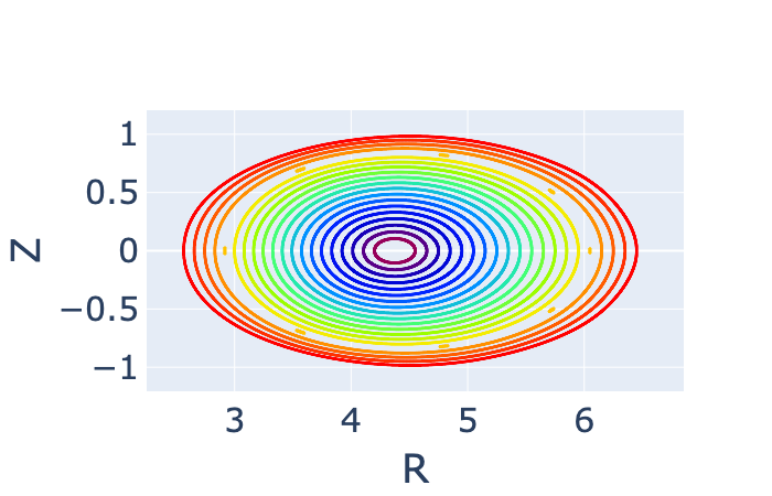
We begin with a boundary given by a rotating ellipse (42) with $a=2$, $b=1$, $R_{0}=5$, and $R_{0,1}=0$. We optimize the boundary with respect to the modes $m\leq 10$ and $|n|\leq 10$. The equilibrium is computed with $p(\psi)=0$ and $I_{T}(\psi)=0$ such that a vacuum field is considered. We arrive at the boundary given in Figure 7. With the addition of the volume constraint, the aspect ratio remains roughly constant (3.54 for the initial boundary and 3.46 for the optimized boundary), so that the well is provided by the shaping of the boundary rather than the Shafranov shift that arises due to the inverse aspect ratio. We note that the optimized surface features triangularity that rotates from outward-pointing with horizontal elongation to inward-pointing with vertical elongation.

To demonstrate the effect of the curvature regularization terms, we examine the optimization with $\lambda_{\kappa}=\lambda_{\overline{\kappa}}=0$. We converge to the boundary shown in Figure 8. As can be seen, regions of large curvature are exhibited, including a dimple-like feature on the inboard side and a concave “pinching” feature. Again the aspect ratio remains roughly constant (3.46).

We can understand the geometric dependence of the magnetic well by considering the expression for $V^{\prime\prime}(\psi)$ on the axis that arises from the near-axis expansion in the inverse coordinate representation (Landreman & Jorge 2020),

$\displaystyle V^{\prime\prime}(\psi)\propto\int_{0}^{2\pi}d\varphi_{B}\,\frac{1}{B_{0}^{4}}\left[3(B_{1s}^{2}+B_{1c}^{2})-4B_{0}B_{20}\right],$

(30)

where $\varphi_{B}$ is the Boozer toroidal angle and we have made the assumption of a vacuum field. The field strength near the axis is expanded as,

$$B=B_{0}(\varphi_{B})+r\left[B_{1c}(\varphi_{B})\cos(\vartheta_{B})+B_{1s}(\varphi_{B})\sin(\vartheta_{B})\right]\\ +r^{2}\left[B_{20}(\varphi_{B})+B_{2c}\cos(2\vartheta_{B})+B_{2s}\sin(2\vartheta_{B})\right]+\mathcal{O}\left(r^{3}\right),$$

(31)

where $r\propto\sqrt{\psi}$ is the effective minor radius and $\vartheta_{B}$ is the Boozer poloidal angle.

As can be seen from (A34) in (Landreman & Sengupta 2019), the poloidally-independent shift in the flux surface in the normal direction, $X_{20}$, increases proportional to $B_{20}$. Here, the normal vector is $\hat{\textbf{n}}=\textbf{r}^{\prime\prime}(l)/|\textbf{r}^{\prime\prime}(l)|$, where $\textbf{r}(l)$ is the position vector along the magnetic axis parameterized by the length. In the axisymmetric limit, a positive value of $X_{20}$ indicates a net shift of the surfaces’ geometric center toward a smaller major radius. This correlation between $X_{20}$ and $B_{20}$ is consistent with the statement that a Shafranov shift provides a magnetic well. In Figures 7 and 8 we display the magnetic axis (blue star) and normal vector (black arrow) along with the shapes of several magnetic surfaces for the optimized configurations. While both the unconstrained and constrained optima feature a net shift in the geometric center of the flux surfaces in the normal direction, this is achieved with vastly different shaping of the boundary. Interestingly, both configurations feature negative triangularity at the $\phi=0.5$ $(2\pi/N_{P})$ plane.

We note that $B_{20}$ arises due to other shaping components of the surface (Landreman & Sengupta 2019). In axisymmetry, negative values of $B_{2c}$ contribute to positive (outward-pointing) triangularity ($X_{2c}<0$) ((B11) in (Landreman 2020)). Assuming stellarator symmetry, negative values of $B_{2c}$ contribute to positive values of $B_{20}$ if the surface is vertically elongated, and positive values of $B_{2c}$ contribute to positive values of $B_{20}$ if the surface is horizontally elongated. This implies that positive triangularity coupled with vertical elongation or negative triangularity coupled with horizontal elongation contributes to the magnetic well in axisymmetry. These trends are consistent with the stability analysis of oblate plasmas with negative triangularity (Pogutse & Yurchenko 1982; Kesner et al. 1995; Medvedev et al. 2015). In 3D, the connection between $B_{20}$ and $B_{2c}$ is more complicated ((A41)-(A42) in (Landreman & Sengupta 2019)). Nonetheless, we note that the magnetic well near the axis arises at second order in the expansion parameter, which includes the effects of ellipticity and triangularity. Thus it is not surprising that the optimized boundary with curvature constraints features rotating ellipticity and triangularity.

In comparing the convergence of the optimization with and without the curvature constraints (Figure 9), we see that the presence of the curvature objective prevents some failures of the VMEC code. Each function evaluation that resulted in a VMEC failure is visualized as a “spike” that extends above $|f_{w}-f^{\text{opt}}_{w}|=1$, as we artificially set the value of the objective function to $10^{12}$ at these points. While the constrained optimization still features some VMEC failures (12 vs. 19), the inclusion of the curvature constraints improves the convergence toward the optimum, and a deeper magnetic well is achieved throughout the volume.

We next consider optimization for quasisymmety near the magnetic axis. This is quantified through the objective,

$\displaystyle f_{QS}=\frac{\int_{V_{P}}d^{3}x\,w(\psi)(B-\overline{B})^{2}}{\int_{V_{P}}d^{3}x\,B^{2}},$

(32)

where $\overline{B}=\int_{V_{P}}d^{3}x\,w(\psi)B$ and we take $w(\psi)=e^{-(\psi/\psi_{0})^{2}/0.1^{2}}$. This objective aims to make the field strength constant on the magnetic axis, which is a feature of quasi-axisymmetric and quasi-helically symmetric equilibria. A similar objective function has also been included in optimization for energetic particle confinement (Drevlak et al. 2014). The gradient of this objective function is obtained by computing an equilibrium with the addition of an anisotropic pressure tensor, $\nabla\cdot\textbf{P}=p_{||}\hat{\textbf{b}}\hat{\textbf{b}}+p_{\perp}\left(\textbf{I}-\hat{\textbf{b}}\hat{\textbf{b}}\right)$ with,

	$\displaystyle p_{||}(\psi,B)$	$\displaystyle=\frac{w(\psi)(B-\overline{B})^{2}-f_{QS}w(\psi)B^{2}}{\int_{V_{P}}d^{3}x\,w(\psi)B^{2}}$		(33a)
	$\displaystyle p_{\perp}$	$\displaystyle=p_{||}-B\frac{\partial p_{||}(\psi,B)}{\partial B},$		(33b)

as described in (Paul et al. 2020).

We take our objective function to be,

$\displaystyle f(S_{P})=f_{QS}+\lambda_{\iota}f_{\iota}+\lambda_{\overline{\kappa}}f_{\overline{\kappa}}+\lambda_{\kappa}f_{\kappa}+\lambda_{\mathcal{S}}f_{\mathcal{S}}+\lambda_{R}f_{R},$

(34)

where $\iota_{\text{target}}(\psi)$ is taken to be the initial rotational transform profile. We also take $\lambda_{\iota}=1$, $\lambda_{\overline{\kappa}}=10^{-3}$, $\lambda_{\kappa}=5\times 10^{-2}$, $\kappa_{\text{max},1}=\kappa_{\text{max},2}=10$ m^-1, $w_{\kappa}=1$, $w_{\mathcal{S}}=w_{R}=10^{-1}$, $\lambda_{R}=10^{3}$, $\lambda_{\mathcal{S}}=10^{-1}$, $\mathcal{R}=0.5$ m, and $R_{\text{min}}=0.2$ m. The additional constraint on the rotational transform is required to prevent the surface from becoming axisymmetric to reduce the toroidal ripple on the axis.

We begin with a rotating ellipse boundary with torsion, given by,

	$\displaystyle R(\theta,\phi)=R_{0}+R_{0,1}\cos(\phi)+R_{0,2}\cos(2\phi)$	$\displaystyle+0.5a\left(\cos\left(\theta-N_{P}\phi\right)+\cos(\theta)\right)$
		$\displaystyle-0.5b\left(\cos\left(\theta-N_{P}\phi\right)-\cos(\theta)\right)$		(35a)
	$\displaystyle Z(\theta,\phi)=R_{0,1}\sin(\phi)+Z_{0,2}\cos(2\phi)$	$\displaystyle+0.5b\left(\sin(\theta)+\sin\left(\theta-N_{P}\phi\right)\right)$
		$\displaystyle+0.5a\left(\sin(\theta)-\sin\left(\theta-N_{P}\phi\right)\right),$		(35b)

with $R_{0}=5$, $R_{0,1}=R_{0,2}=0.3$, $a=2$, $b=1$, and $N_{P}=3$. We perform optimization at $\beta=1.2$ % with the profiles shown in Figure 10. We optimize with respect to the modes $m\leq 10$ and $|n|\leq 10$ in a staged approach: first optimizing with respect to $m\leq 3$ and $|n|\leq 3$, then with respect to $m\leq 6$ and $|n|\leq 6$, then with respect to the full set of modes.

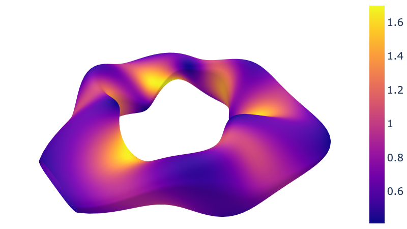
We display the magnetic field strength on the initial and optimized boundaries in Figure 11. We note the initial configuration features a large toroidal variation of the field strength, with increased field strength near the “corners” that arise due to the axis’s large torsion. Although the axis ripple figure of merit (32) reduces the toroidal variation of the field strength on the axis, which must vanish in both quasi-axisymmetry and quasi-helical symmetry, we find that the optimized magnetic field is driven closer to quasi-axisymmetry.

We remark that a design based solely on the objective (32) may be limited in that quasisymmetry is not targeted away from the axis. We therefore quantify the departure from quasisymmetry in the two configurations in two additional ways. The first is through the figure of merit,

$\displaystyle f_{TP}(\psi)$

$\displaystyle=\frac{\left\langle\left\rvert\frac{\partial B}{\partial\theta}\frac{\partial}{\partial\phi}\left(\textbf{B}\cdot\nabla B\right)-\frac{\partial B}{\partial\phi}\frac{\partial}{\partial\theta}\left(\textbf{B}\cdot\nabla B\right)\right\rvert\right\rangle_{\psi}}{\langle B^{3}\rangle_{\psi}/r_{\text{minor}}(\psi)},$

(36)

where $r_{\text{minor}}(\psi)=\sqrt{A(\psi)/\pi}$ is the averaged minor radius of a flux surface where $A(\psi)$ is the toroidally averaged cross-sectional area. (This is the same definition of the minor radius used in the VMEC code.) The flux-surface average of a quantity $Q$ is,

$\displaystyle\langle Q\rangle_{\psi}=\frac{\int_{0}^{2\pi}d\theta\int_{0}^{2\pi}d\phi\,Q\sqrt{g}}{\int_{0}^{2\pi}d\theta\int_{0}^{2\pi}d\phi\,\sqrt{g}},$

(37)

where $\sqrt{g}=\left(\nabla\psi\times\nabla\theta\cdot\nabla\phi\right)^{-1}$ is the flux coordinate Jacobian. Eq. (36) is a normalized figure of merit which employs the triple product form for quasisymmetry (Helander 2014; Rodriguez et al. 2020),

$\displaystyle\nabla\psi\times\nabla B\cdot\nabla\left(\textbf{B}\cdot\nabla B\right)=0,$

(38)

and allows us to quantify the quasisymmetry error without specifying the helicity of the symmetry. We also perform a Boozer coordinate ($\psi$,$\vartheta_{B}$,$\varphi_{B}$) transformation (Sanchez et al. 2000) to obtain the Fourier harmonics of the field strength,

$\displaystyle B(\psi,\vartheta_{B},\varphi_{B})=\sum_{m,n}B_{m,n}\cos(m\vartheta_{B}-n\varphi_{B}).$

(39)

The deviation from quasi-axisymmetry can then be quantified as,

$\displaystyle f_{QA}(\psi)$

$\displaystyle=\sqrt{\frac{\sum_{m,n\neq 0}B_{m,n}(\psi)^{2}}{\sum_{m,n}B_{m,n}(\psi)^{2}}}.$

(40)

Although quasisymmetry was only targeted on the axis, we reduce the quasisymmetry error throughout the volume with respect to both metrics without introducing a reduction in the rotational transform (Figure 12).

References

- Anderson et al. (1995) Anderson, F. S. B., Almagri, A. F., Anderson, D. T., Matthews, P. G., Talmadge, J. N. & Shohet, J. L. 1995 The Helically Symmetric eXperiment,(HSX) goals, design and status. Fusion Technology 27 (3T), 273–277.
- Antonsen et al. (2019) Antonsen, T., Paul, E. J. & Landreman, M. 2019 Adjoint approach to calculating shape gradients for three-dimensional magnetic confinement equilibria. Journal of Plasma Physics 85 (2).
- Beidler et al. (1990) Beidler, C., Grieger, G., Herrnegger, F., Harmeyer, E., Kisslinger, J., Lotz, W., Maassberg, H., Merkel, P., Nührenberg, J., Rau, F. & others 1990 Physics and engineering design for Wendelstein VII-X. Fusion Technology 17 (1), 148–168.
- Carlen et al. (2005) Carlen, M., Laurie, B., Maddocks, J. H. & Smutny, J. 2005 Biarcs, global radius of curvature, and the computation of ideal knot shapes. In Physical and Numerical Models in Knot Theory: Including Applications to the Life Sciences, pp. 75–108. World Scientific.
- Carlton-Jones et al. (2020) Carlton-Jones, A., Paul, E. J. & Dorland, W. 2020 Computing the shape gradient of stellarator coil complexity with respect to the plasma boundary. arXiv preprint arXiv:2011.03702 .
- Cooper et al. (1992) Cooper, W. A., Hirshman, S. P., Merazzi, S. & Gruber, R. 1992 3D magnetohydrodynamic equilibria with anisotropic pressure. Computer Physics Communications 72 (1), 1.
- Dekeyser (2014) Dekeyser, W. 2014 Optimal plasma edge configurations for next-step fusion reactors. PhD thesis, Katholieke Universiteit Leuven.
- Drevlak et al. (2018) Drevlak, M., Beidler, C. D., Geiger, J., Helander, P. & Turkin, Y. 2018 Optimisation of stellarator equilibria with ROSE. Nuclear Fusion 59 (1), 016010.
- Drevlak et al. (2013) Drevlak, M., Brochard, F., Helander, P., Kisslinger, J., Mikhailov, M., Nührenberg, C., Nührenberg, J. & Turkin, Y. 2013 ESTELL: A quasi-toroidally symmetric stellarator. Contributions to Plasma Physics 53 (6), 459–468.
- Drevlak et al. (2014) Drevlak, M. C., Geiger, J., Helander, P. & Turkin, Y. 2014 Fast particle confinement with optimized coil currents in the W7-X stellarator. Nuclear Fusion 54 (7), 073002.
- Emmerich et al. (2002) Emmerich, Michael, Giotis, Alexios, Özdemir, Mutlu, Bäck, Thomas & Giannakoglou, Kyriakos 2002 Metamodel—assisted evolution strategies. In International Conference on parallel problem solving from nature, pp. 361–370. Springer.
- Gelsey (1995) Gelsey, Andrew 1995 Intelligent automated quality control for computational simulation. AI EDAM 9 (5), 387–400.
- Gelsey et al. (1998) Gelsey, Andrew, Schwabacher, Mark & Smith, Don 1998 Using modeling knowledge to guide design space search. Artificial Intelligence 101 (1-2), 35–62.
- Giuliani et al. (2020) Giuliani, A., Wechsung, F., Cerfon, A., Stadler, G. & Landreman, M. 2020 Single-stage gradient-based stellarator coil design: Optimization for near-axis quasi-symmetry. arXiv preprint arXiv:2010.02033 .
- Gonzalez & Maddocks (1999) Gonzalez, O. & Maddocks, J. H. 1999 Global curvature, thickness, and the ideal shapes of knots. Proceedings of the National Academy of Sciences 96 (9), 4769–4773.
- Greene et al. (1986) Greene, J. M., MacKay, R. S. & Stark, J. 1986 Boundary circles for area-preserving maps. Physica D: Nonlinear Phenomena 21 (2-3), 267–295.
- Helander (2014) Helander, P. 2014 Theory of plasma confinement in non-axisymmetric magnetic fields. Reports on Progress in Physics 77 (8), 087001.
- Henneberg et al. (2019) Henneberg, SA, Drevlak, M, Nührenberg, C, Beidler, CD, Turkin, Y, Loizu, J & Helander, P 2019 Properties of a new quasi-axisymmetric configuration. Nuclear Fusion 59 (2), 026014.
- Hirshman & Whitson (1983) Hirshman, S. P. & Whitson, J. C. 1983 Steepest-descent moment method for three-dimensional magnetohydrodynamic equilibria. The Physics of Fluids 26 (12), 3553–3568.
- Hudson et al. (2012) Hudson, S. R., Dewar, R. L., Dennis, G., Hole, M. J., McGann, M., Von Nessi, G. & Lazerson, S. 2012 Computation of multi-region relaxed magnetohydrodynamic equilibria. Physics of Plasmas 19 (11), 112502.
- Johnson (2014) Johnson, S. G. 2014 The NLopt nonlinear-optimization package.
- Kesner et al. (1995) Kesner, J., Ramos, J. J. & Gang, F.-Y. 1995 Comet cross-section tokamaks. Journal of Fusion Energy 14 (4), 361–371.
- Landreman (2020) Landreman, M. 2020 Figures of merit for stellarators near the magnetic axis, arXiv: 2012.00865.
- Landreman & Jorge (2020) Landreman, M. & Jorge, R. 2020 Magnetic well and Mercier stability of stellarators near the magnetic axis. Journal of Plasma Physics 86 (5), 905860510.
- Landreman & Sengupta (2019) Landreman, M. & Sengupta, W. 2019 Constructing stellarators with quasisymmetry to high order. Journal of Plasma Physics 85 (6).
- Lazerson et al. (2020) Lazerson, Samuel, Schmitt, John, Zhu, Caoxiang, Breslau, Joshua & STELLOPT Developers 2020 STELLOPT. https://github.com/PrincetonUniversity/STELLOPT.
- Lemaréchal (1982) Lemaréchal, Claude 1982 Numerical experiments in nonsmooth optimization. .
- Lewis & Overton (2009) Lewis, Adrian S & Overton, Michael L 2009 Nonsmooth optimization via BFGS. Submitted to SIAM J. Optimiz pp. 1–35.
- McGreivy et al. (2021) McGreivy, N., Hudson, S.R. & Zhu, C. 2021 Optimized finite-build stellarator coils using automatic differentiation. Nuclear Fusion 61 (2), 026020.
- Medvedev et al. (2015) Medvedev, S. Y., Kikuchi, M., Villard, L., Takizuka, T., Diamond, P., Zushi, H., Nagasaki, K., Duan, X., Wu, Y., Ivanov, A. A. & others 2015 The negative triangularity tokamak: stability limits and prospects as a fusion energy system. Nuclear Fusion 55 (6), 063013.
- Meiss (1992) Meiss, J. D. 1992 Symplectic maps, variational principles, and transport. Reviews of Modern Physics 64 (3), 795.
- Mercier (1964) Mercier, C. 1964 Equilibrium and stability of a toroidal magnetohydrodynamic system in the neighbourhood of a magnetic axis. Nuclear Fusion 4 (3), 213.
- Mercier & Luc (1974) Mercier, C. & Luc, H. 1974 The MHD approach to the problem of plasma confinement in closed magnetic configurations. Lectures in Plasma Physics, Commission of the European Communities, Luxembourg .
- Miner Jr et al. (2001) Miner Jr, W. H., Valanju, P. M., Hirshman, S. P., Brooks, A. & Pomphrey, N. 2001 Use of a genetic algorithm for compact stellarator coil design. Nuclear Fusion 41 (9), 1185.
- Mynick et al. (2002) Mynick, H. E., Pomphrey, N. & Ethier, S. 2002 Exploration of stellarator configuration space with global search methods. Physics of Plasmas 9 (3), 869–876.
- Nocedal & Wright (2006) Nocedal, J. & Wright, S. J. 2006 Numerical Optimization. Springer.
- Nührenberg & Zille (1988) Nührenberg, J. & Zille, R. 1988 Quasi-helically symmetric toroidal stellarators. Physics Letters A 129 (2), 113–117.
- Oymak & Soltanolkotabi (2018) Oymak, S. & Soltanolkotabi, M. 2018 Overparameterized nonlinear learning: Gradient descent takes the shortest path? arXiv preprint arXiv:1812.10004 .
- Paul (2020) Paul, E. J. 2020 Adjoint methods for stellarator shape optimization and sensitivity analysis. arXiv preprint arXiv:2005.07633 .
- Paul et al. (2019) Paul, E. J., Abel, I. G., Landreman, M. & Dorland, W. 2019 An adjoint method for neoclassical stellarator optimization. Journal of Plasma Physics 85 (5).
- Paul et al. (2020) Paul, E. J., Antonsen, T., Landreman, M. & Cooper, W. A. 2020 Adjoint approach to calculating shape gradients for three-dimensional magnetic confinement equilibria. Part 2. Applications. Journal of Plasma Physics 86 (1).
- Paul et al. (2018) Paul, E. J., Landreman, M., Bader, A. & Dorland, W. 2018 An adjoint method for gradient-based optimization of stellarator coil shapes. Nuclear Fusion 58 (7), 076015.
- Pogutse & Yurchenko (1982) Pogutse, O. & Yurchenko, E. 1982 Reviews of Plasma Physics. Consultants Bureau, New York .
- Rasheed et al. (1997) Rasheed, Khaled, Hirsh, Haym & Gelsey, Andrew 1997 A genetic algorithm for continuous design space search. Artificial Intelligence in Engineering 11 (3), 295–305.
- Rodriguez et al. (2020) Rodriguez, E., Helander, P. & Bhattacharjee, A. 2020 Necessary and sufficient conditions for quasisymmetry. Physics of Plasmas 27 (6), 062501.
- Sanchez et al. (2000) Sanchez, R., Hirshman, S. P., Ware, A. S., Berry, L. A. & Spong, D. A. 2000 Ballooning stability optimization of low-aspect-ratio stellarators. Plasma Physics and Controlled Fusion 42 (6), 641.
- Sauer (2012) Sauer, Timothy 2012 Numerical Analysis. Pearson.
- Smutny (2004) Smutny, J. 2004 Global radii of curvature, and the biarc approximation of space curves: In pursuit of ideal knot shapes. PhD thesis, EPFL.
- Taylor (1965) Taylor, J. B. 1965 Simple toroidal magnetic field with negative . The Physics of Fluids 8 (6), 1203–1205.
- Walker (2016) Walker, S. W. 2016 Shape optimization of self-avoiding curves. Journal of Computational Physics 311, 275–298.
- Wesson & Campbell (2011) Wesson, J. & Campbell, D. J. 2011 Tokamaks, International Series of Monographs on Physics, vol. 149. Oxford University Press.
- Zarnstorff et al. (2001) Zarnstorff, M. C., Berry, L. A., Brooks, A., Fredrickson, E., Fu, G. Y., Hirshman, S., Hudson, S., Ku, L. P., Lazarus, E., Mikkelsen, D. & others 2001 Physics of the compact advanced stellarator NCSX. Plasma Physics and Controlled Fusion 43 (12A), A237.
- Zhu et al. (2018) Zhu, C., Hudson, S. R., Song, Y. & Wan, Y. 2018 New method to design stellarator coils without the winding surface. Nuclear Fusion 58, 016008.