Leptonic Flavor Changing Processes and in the Twin Higgs Models
Abstract
Heavy neutrinos are usually introduced to accommodate tiny neutrino masses via seesaw mechanism, or to alleviate the cosmology problem, and there may exist charged Higgses which couple to the leptons with different flavors. These two features can both appear in the Twin Higgs models. What interests us is that such new particles and interactions may lead to new contributions to the lepton flavor violating processes and . We find that current experimental data can constrain the parameter spaces and certain lepton flavor violating processes can possibly be tested by the next generation experiments.
Keywords:
lepton flavor violation, branching ratio, Twin Higgs modelspacs
13.38.Dg,14.66.-z,12.60.-iI Introduction
In the Standard Model (SM), the conservation of individual lepton flavor numbers and the presentation of the GIM mechanism GIM-1970 guarantee that the cross sections and/or branching ratios of the lepton flavor violating (LFV) processes are tiny. For example, the SM predicts the branching ratio SMljlig to be very small, which would never be probed in experiments. Therefore, it will be an obvious evidence of new physics beyond the SM if we observe any signature of the LFV processes in future experiments, so LFV processes are very efficient in exploring new physics beyond the SM. As the upper bounds of the LFV processes by current experiments have been given with impressive accuracy, it is interesting to explore whether theoretical predictions of a typical new physics model can agree with the experimental results. Many works have been completed to look for the LFV processes , in new physics models, see e.g. bSM1; bSM2; bSM3; bSM4; bSM5; bSM6; 1701.00947; 1812.03860; 1812.02449; 1912.05900; 0506070; 0307126; 0206056.
It is well known that the neutrino oscillation experiments neutrino1; neutrino2; neutrino3; neutrino4; neutrino5; neutrino6; neutrino7; neutrino8; neutrino9 indicate that neutrinos possess tiny masses and can convert into each other, so individual lepton flavor numbers may be violated at the electroweak scale. Weinberg’s effective dimension-5 operator is the lowest one that can generate tiny Majorana-type neutrino masses. Such an operator can be tree level ultraviolet(UV)-completed to obtain three types of tree-level seesaw mechanism: type I seesaw type I, involving the exchange of right-handed neutrinos; type II seesaw type II, involving the exchange of scalar triplet; type III type III, involving the exchange of fermion triplet. The neutrino seesaw mechanisms can also be embedded into various well motivated new physics models to accommodate the neutrino masses, such as the Twin Higgs (TH) models litt-hier1.
TH models, which usually extend the SM with a copy, can stabilize the Higgs mass from quadratic divergent quantum corrections by a discrete symmetry. The new particles, which are related to the SM particles by this discrete symmetry, do not carry the SM color charges and can hardly be produced and detected at the colliders, ameliorating the stringent constraints on the mass of the top partner by the Large Hadron Collider(LHC) parti-tev.
Although TH models are theoretically appealing, they encounter difficulties by cosmological considerations. In the simplest realization of TH litt-hier1 models, the twin particles will eventually transfer their entropies into twin photons and twin neutrinos, which behave as extra radiation components, increasing the SM prediction by an additional amount 1611.07975-neff_mth, which deviates the observations neff_exp1; neff_exp2, where is effective number of (light) neutrino species.
Various modifications are proposed to reduce the value and solve the problems of TH models. For example, the first and second generations of twin fermions as well as twin photon can be absent modif-mth1; Or in some realizations, the twin neutrinos, and even twin photons can be heavy modif-mth2; modif-mth3-1703.06884; modif-mth4; modif-mth5-1905.00861. Asymmetric entropy production can be possible after the twin and SM sectors decouple 1611.07975-neff_mth; modif-mth3-1703.06884; modif-mth6; modif-mth7.
The seesaw extension of TH models usually predicts massive twin neutrino masses to lower the effective degrees of freedom contributed by the twin sector modif-mth3-1703.06884. These models can also introduce extra massive right-handed neutrinos in both sectors of SM and the twin 1611.07975-neff_mth to generate the tiny neutrino masses. Typical lepton-flavor-changing couplings will appear via these mechanisms, which may lead to interesting phenomenological consequences, so we try to study the lepton flavor violating (LFV) processes , induced by these new couplings in this work.
The paper is organized as follows. Section II briefly gives the new LFV couplings in TH models. In section III, the amplitudes and the branching ratios of rare LFV processes , will be calculated, respectively. The corresponding numerical results are also shown in this section. The conclusion will be given in Section IV.
II The Lepton Flavor Violating Couplings in the twin higgs models
In TH framework, the SM particles and their copies are related by the discrete twin symmetry. To contain a residual custodial symmetry, the global symmetry of the Higgs sector in the simplest realization can be taken as or Barbieri:2015lqa; Batra:2008jy; 1501.07890; 1905.02203. The SM Higgs doublet is a part of the pseudo-Nambu-Goldstone bosons (pNGBs), which arises from the spontaneously breaking of the global ( ) symmetry into ( ). The neutral Higgs mass, under the joint action of the global symmetry and the discrete twin symmetry, is protected from one loop quadratic divergence.
Besides the SM-like neutral Higgs, there would be charged Higgses. In some TH models, for different goals, extra scalars will be introduced. For example, in Ref.1702.04399, a singlet charged scalar is introduced to provide suitable neutrino masses via couplings to the right-handed neutrinos, while in Refs.modif-mth4; modif-mth5-1905.00861, a new scalar is added to have the similar effect in the couplings with the leptons. Another possiblity for the extra charged scalars to appear in the particle list is due to the enlarging breaking mode. To keep the breaking smallest, the economical breaking choices are chosen as above but it can be otherwise in some situation. For example, the breaking modes can be or 2202.01228 (the former is for SM sector, while the latter, for twin sector).
After the global breaking such as , the seven pNGBs can be parameterized via the decomposition under as
| (1) |
where is the Goldstone scale, TeV, and (), and is assumed to be the SM-like Higgs. The SM gauge fields acquire the typical masses proportional to the scale of electroweak symmetry breaking, .
In case additional contributions to of TH models cause difficulties in cosmology11 1 In scenarios with multiple dark matter components, small contributions to can possibly solve the discrepancy between the value of extracted from local measurements versus CMB data., one can impose another portal, such as the neutrino portal to reduce the to the acceptable level. However, new flavor-changing couplings can be generated via the mixing between the SM neutrino and the twin neutrino and they can be given as modif-mth3-1703.06884,
| (2) | |||||
where , and is the mixing angle between ordinary neutrino and twin neutrino . Note that there is actually not only the mixing, but also the Pontecorvo-Maki-Nakagawa-Sakata (PMNS) mns-maki-1962; 0712.4019 matrix elements. Here for simplicity we denote to represent the effect of all these parameters. So does the following parameter .
On the other hand, the LFV couplings can also be induced from the typical neutrino seesaw extension of the TH models via introducing the massive right-handed neutrino 1611.07975-neff_mth; 1905.02203,
| (3) | |||||
in both the SM(denoted by ) and twin sectors(denoted by ).
From Eqs. (2) (3), we can see the particles which induce the LFV couplings could be gauge bosons and the new charged scalars with the twin neutrinos or the right-handed neutrinos . Note that there are two kinds of neutrinos: In general, the twin neutrinos can couple to gauge bosons together with the leptons, and the right-handed neutrinos couple to the charged Higgs with the leptons. From the following discussion, we can see that they both are much heavier than the ordinary neutrinos, so we will call them ”heavy neutrinos” when not causing confusion.
In the process of lowering the decoupling temperature and potentially reducing the contribution to , the constraint on the mixing of the ordinary neutrino and twin neutrino is mainly from the decay of the twin neutrino to the ordinary neutrino , and the semi annihilations , with the usual range scope of the value of the decoupling temperature, modif-mth3-1703.06884; 1604.02458, and the favourable space can be with twin neutrino mass of GeV, which is the optimal value for the thermal decoupling between the SM and the twin sectors.
Normally, to provide the tiny neutrino masses, we need massive right-handed neutrinos, as those in type I seesaw. The charged Higgs mass is discussed in references such as 0611015-su; lfv-lrth; charged-neutral-mass and our previous worksworks-inv-chaghiggs. According to the references, the mass difference between the charged Higgs boson and the neutral heavy Higgs boson should be less than GeV, i.e., GeV, and in general, the mass of the neutral heavy Higgs boson is larger than that of the SM-like Higgs. In our discussion and calculation we can take and in the following ranges
| (4) |
As for the Yukawa couplings , according to the relationship of the masses of the ordinary neutrino and the right-handed neutrino, 1611.07975-neff_mth, we can estimate the range should be if the right-handed neutrino masses are in the order of TeV and the ordinary neutrino masses are in the range of eV. This is much larger than the estimation in Ref.1611.07975-neff_mth since it assumes that the right-handed neutrinos are in the GeV order.
III The processes and
In this section, we analyze the branching ratios of certain LFV processes in the TH model, including , , , , .
III.1 The width and the Branching ratios of the rare decay

The Feynman diagrams for , which can be mediated by the gauge bosons and the charged Higgs, are shown in Fig.1, with the initial and the final leptons and , respectively.
The Lorentz structure of is written as the matrix element of the electromagnetic current between incoming and outgoing fermion states with momentum and spin and , respectively,
| (5) |
where , and is the photon momentum, , . For the amplitude of , the first term in Eq.(5) will disappear due to the electromagnetic gauge invariance, . That can be seen as following. Multiplying Eq.(5) by , the left side is equal to zero. For , the second term of the right side vanishes, and thus the first term of the same side equals to zero, i.e, . This term corresponds to the self energy diagrams in Fig.1(c)(d) and they do not contribute to the amplitude of the decay .
Therefore, the total effective amplitude of , which is contributed by the gauge bosons and the charged Higgs with the heavy neutrinos, can be written as
| (6) |
where is the mass of the initial(final) state lepton, and are the momentums of the initial, final state lepton and the photon, respectively, and is the polarization vector of the photon. Note that the final state lepton masses are neglected, .
| (7) |
where () is the couplings of the charged gauge bosons(Higgs) to the fermions, as previously stated. Since gauge bosons couple to twin neutrinos, and charged Higgs to right-handed neutrinos, so the terms with the ”” superscript are the contributions from twin neutrinos, and ”” superscript ones, from right-handed neutrinos.
In the above equation, () are the one-loop three point functions looptools, and for , ; , .
So, the decay width is given as
| (8) |
III.1.1 The process
The width of the dominant muon-decay mode is given as,
| (9) |
where is the Fermi coupling constant. So the branching ratios of the rare decay is given by
| (10) |


For the third figure of Fig.2, the value range of Y-axis is , in the same order, so we let it vary between to . For the last figure of Fig.2, the number labeled next to the Y-axis variable is the middle value of the narrow range of the Y-axis:().
In the lower part of Fig.2, we can see the contributions to the branching ratios from the masses of the charged Higgs and the neutrinos are small and oscillatory in the narrow ranges.22 2 The new particles, such as charged Higgs, right-handed neutrinos and the heavy fermions, are in the inner lines of the Fig. 1, and the contributions are expressed by complex integral function . According to the definition of the integral function , there are terms such as in the denominator( is a very tiny real number), and in general calculation, the term is neglected, but it will play a crucial role when the momentums are close to the masses, ensuring the results converging. This situation may lead to oscillating results in some mass range.33 3 Generally speaking, the contribution decreases with the increasing masses. In Fig.2, since the mass ranges are not large enough, this decreasing effect is not obvious. But it is impossible for the contributions to oscillate regularly to very large masses. Even so, with very narrow varying range, from the last figure of Fig.2, we can still see the decreasing branching ratio with the increasing twin neutrino mass. Moreover, they are all smaller than the detected level given in Eq.(11). Thus in the following, we will take the masses as fixed values.
In the upper part of Fig.2, we show the dependence of the branching ratios on the couplings, , from which we can see that the branching ratios increase monotonously along with the increasing couplings, and that they may arrive at the detectable level, so the couplings play a more important role on the branching ratios in comparison with the mass parameters.
The detectable experimental upper bound is given by 1605.05081; 1107.5547
| (11) |
From this constraints, the approximate range of the couplings can be given as
| (12) |
But if it is possible for the processes to be detected in experiments, the couplings should be larger than , respectively, which would be stringent constraints.
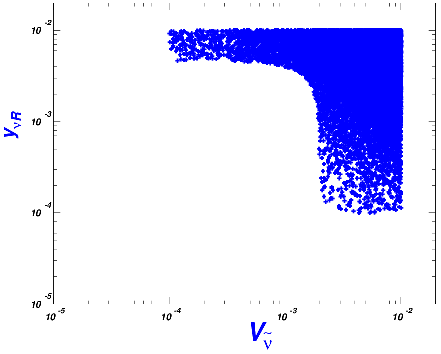
The above constraints are derived from the independent influence of these two couplings on the branching ratio. We can also consider the points allowed to exist in the scan parameter space when the branching ratios are greater than the upper limit of the experimental upper bound. We scan the coupling parameters in the ranges:() and their possible allowed points are shown in Fig.3, from which we can see that, for this process, large or is favorable to be detected at the colliders.
III.1.2 The processes and
As for the and , the total widths are different from that of the muon since the can decay not only into , but also into . Besides, it can decay hadronically since lepton is heavier than the light quarks. Taking into account the unitarity of the quark mixing matrix, , one can easily get the lowest-order width (see e.g. Ref. 1310.7922 and the Refs. in it),
| (13) |
so the branching ratios of and can be written as,
| (14) |
Note that the notation is the same as Eq.(7) except that the leptons involved in their coupling coefficients are different: The former is with , and the latter is with or , but the expressions are the same since there will be no confusion with each other.
The experimental upper bounds are taubound-0908.2381,
| (15) |
The two LFV processes and , are almost the same. What makes difference is the final lepton mass, but in the crude estimation, we can neglect the final lepton masses, i.e, . Therefore, in the following we will just consider the former.
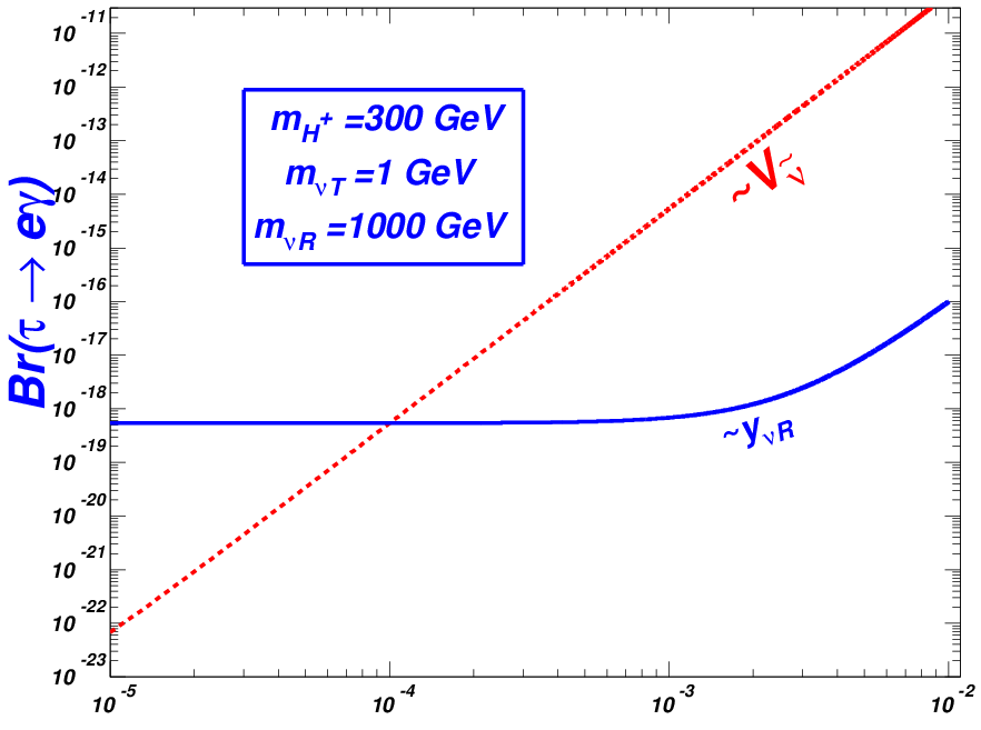
In Fig.4, we show the branching ratios of vary with the couplings and with the fixed masses of the twin neutrino, right-handed neutrino and the charged Higgs, since they are not sensitive to the varying of the mass parameters. We take () when the variable is (). Fig.4 shows that the branching ratios depend greatly on the couplings. However, even when or is close to , which is quite large for the ranges discussed in Sec. II, the branching ratios can still not reach the detectable sensitivity in experiments shown in Eq.(15). Thus this process can not provide constraints to the couplings for the time being, so we will not discuss it further.
III.2 The decay and ()
III.2.1 The decay and mediated by new neutral gauge bosons
We now discuss the three body decays of the leptons mediated by the new neutral gauge bosons. The so-called new neutral gauge bosons mean the partners of the SM gauge bosons or the extra vector gauge boson introduced by the twin Higgs modes, such as Ref. 1811.05977, which adds a singleton vector to link the SM and the twin gauge sector. Their couplings to the leptons can be written in a general form as
| (17) |
where the gauge boson is denoted as , and the superscript and denote the parts of vector and axis vector of the boson couplings to the leptons. We will check the contribution from the new gauge bosons to simply estimate the parameter limits.
On the other hand, an important reason to consider the gauge boson effect on the tree-level decay process is that the contribution mediated by the neutral Higgs scalar is much smaller than that of the neutral gauge boson, since the lepton Yukawa couplings i.e, , should be much smaller than the gauge coupling.
Since neutral gauge boson is much heavier than muon, the width of the three-body decay can be written as
| (18) | |||||
where , , is the mass of the gauge boson, is a kinematic-spin factor common to all decay modes mediated by the neutral vector boson, while ( ) and are the electroweak coupling and the boson mass, respectively.
Thus via the same idea, the three-body decay of the lepton involving vector gauge bosons in the intermediate state can be written as
| (19) | |||||
Note that in the above formulas, the final lepton masses have been neglected.


The dependence of the branching ratios on the parameters and the mediator gauge boson mass are given in Fig.5 for and . We find that the branching ratios can account for the the experimental bounds Eq.(16) in quite a large parameter space with a not too large extra new neutral gauge boson, especially for decay .
According to the constraints in Eq.(16), to probe the processes, the lower bounds of the couplings can be estimated as
| (20) |
with GeV. The main reason of the bound on is stronger than in Eq.(20) for a fixed is that, according to Eq.(16), to be detected in the experiments, the needed branching ratio of should be four orders smaller than that of , while their branching ratios are almost in the same order, just as shown in Fig.5. And from Fig.5 we can also see that the branching ratios increase with the increasing couplings. Thus can be much smaller than for the processes to be probed.
At the same time, the branching ratio of the former is about five times that of the latter. So the bound on is much stronger, which would be a good feature to probe the new gauge boson via the decay since in many models, a small coupling is much more viable.
III.2.2 The decay and mediated by the charged scalar Higgs and the right handed neutrino at the one-loop level
Since there are no tree-level contributions to the decay modes by the charged bosons and Higgs, some works, such as Refs. 1702.04399; 1909.12147; 1909.02044, consider these processes at the one-loop level. For completion, we will refer to the above references to check the contributions from the charged Higgs and the charged gauge bosons with the extra heavy neutrino.
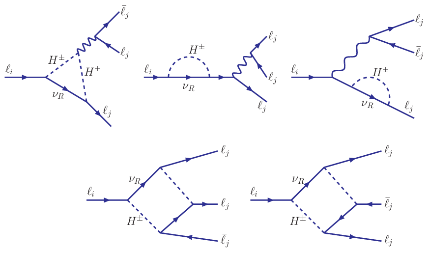
The couplings between the charged Higgs, the charged gauge bosons with the extra heavy neutrinos and the charged leptons can induce the three-body decay of the massive charged leptons at one-loop level. Typical Feynman diagrams are shown in Fig.6 and the branching ratio can be found in the Appendix.
With fixed masses for the charged scalar Higgs and the heavy neutrinos, the branching ratios at the one-loop level are shown in Fig.7, in which () is the coupling of the charged Higgs to the lepton () and the right-handed neutrino, similar to in Eq.(3), but now distinguished for different flavors. We can see that the decay rates are still below the detection sensitivity in Eq.(16) even if we choose the couplings to be . Similar discussions can be given for the same three-body decays mediated by the gauge bosons and the heavy neutrinos at one-loop level. We, however, neglect such processes since their contributions are too small compared to the experimental bounds.

IV Conclusion
We discuss the possible effects of the new exotic fields together with the right-handed neutrinos and gauge bosons with the twin neutrinos in the TH models on the LFV processes and , respectively.
From the discussion given above, with the assumption of degenerate neutrinos for simplification, we can draw the following conclusions:
- •
In some parameter space such as or , the decay channel may arrive at the detectable level. On the other hand, if the experiments can not find any signal of this channel, since the decay is sensitive to the couplings and , this may provide constraints on the parameters in models of this kind.
- •
Similarly, the three body decay channel mediated by the neutral gauge boson may arrive at the the detection level of the experiments, while those mediated via the charged Higgs and the gauge bosons at the one-loop level can not be possible to be detected in most parameter space.
- •
But this is not true for and decay channels. They cannot be probed in the whole possible parameter space.
Therefore, we conclude that the LFV processes of TH models may arrive at the detectable level in a large parameter space, and they may shed light on the constraints of the models or even to find some signal of the models.
Acknowledgments
This work was supported by the National Natural Science Foundation of China(NSFC) under grant 11675147,12075213, 11775012, by the Key Project by the Education Department of Henan Province under grant number 21A140025, by the Fundamental Research Cultivation Fund for Young Teachers of Zhengzhou University(JC202041040) and the Academic Improvement Project of Zhengzhou University.
Appendix A
The branching ratio of mediated by charged Higgs can be written as1702.04399; 1909.12147
| (21) |
where is the dipole contribution,
| (22) |
where () () is the couplings of the charged Higgs to the lepton () and the right-handed neutrino, the mass of heavy Higgs () and . Expression of will be given shortly. The coefficients and are the non-dipole contributions from the penguin and the box diagrams, respectively, which read
| (23) |
and
| (24) |
Note that only one flavor of (mediated) neutrino is assumed.
| (25) | ||||
| (26) | ||||
| (27) | ||||
| (28) |
and
| (29) |
References
- (1)
- (2) S. L. Glashow, J. Iliopoulos and L. Maiani, Phys. Rev. D 2, (1970) 1285.
- (3)
S. Petcov, Sov. J, Nucl. Phys. 25, (1977) 340, [Yad. Fiz. 25, 641 (1977)] Erratum: [Sov. J. Nucl.
Phys. 25, 698 (1977)] Erratum: [Yad. Fiz. 25, 1336 (1977)];
T. P. Cheng and L. F. Li, Gauge Theory Of Elementary Particle Physics, Oxford, Uk: Clarendon (1984) 536 P. (Oxford Science Publications);
L. Calibbi and G. Signorelli, Riv. Nuovo Cim. 41, 1 (2018), 1709.00294; G. Hernandez-Tome, G. Lopez Castro, P. Roig, Eur. Phys. J. C79,(2019) 84, Eur. Phys. J. C 80, (2020) 438 (erratum), arXiv:1807.06050. - (4) J.Chang, K. Cheung, H. Ishida et al, JHEP 1710, (2017) 039, arXiv:1707.04374.
- (5) T. A. Chowdhury and S. Nasri, Phys.Rev. D 97, (2018) 075042, arXiv:1801.07199.
- (6) J. L. Diaz-Cruz, J. J. Toscano, Phys. Rev. D 62, (2000) 116005, arXiv:hep-ph/9910233.
- (7) T. Han, D. Marfatia, Phys. Rev. Lett. 86, (2001) 1442, arXiv: hep-ph/0008141.
- (8) K. Agashe, R. Contino, Phys. Rev. D 80, (2009) 075016, arXiv:0906.1542.
- (9) S. Casagrande et al., JHEP 10, (2008) 094, arXiv:0807.4937.
- (10) Guo-Li Liu, Fei Wang, Kuan Xie, Xiao-Fei Guo, Phys. Rev. D96, (2017) 035005, arXiv:1701.00947.
- (11) Jinlei Yang, T. Feng, Y. Yan, Wei Li, S. Zhao, H. Zhang, Phys. Rev. D 99, (2019) 015002, arXiv:1812.03860.
- (12) Xiaofang Han, Tianjun Li, Lei Wang, Yang Zhang, Phys. Rev. D 99, (2019) 095034, arXiv:1812.02449.
- (13) Mario W. Barela, V. Pleitez, Phys. Rev. D 101, (2020) 015024, arXiv:1912.05900.
- (14) Chongxing Yue, Z. Zong, Li Zhou, Shuo Yang, Phys. Rev. D 71, (2005) 115011, arXiv:hep-ph/0506070.
- (15) Junjie Cao, Zhaohua Xiong, Jin Min Yang, Eur. Phys. J. C 32, (2004) 245, arXiv:hep-ph/0307126.
- (16) Deirdre Black, Tao Han, Hong-Jian He, Marc Sher, Phys. Rev. D 66, (2002) 053002, arXiv:hep-ph/0206056.
- (17) K. Abe et al (T2K Collab.), Phys. Rev. Lett. 107, (2011) 041801.
- (18) P. Adamson et al (MINOS Collab.), Phys. Rev. Lett. 107, (2011) 181802.
- (19) Y. Abe et al (DOUBLE-CHOOZ Collab.), Phys. Rev. Lett. 108, (2012) 131801.
- (20) F. An et al (DAYA-BAY Collab.), Phys. Rev. Lett. 108, (2012) 171803.
- (21) J.Ahn et al (RENO Collab.), Phys. Rev. Lett. 108, (2012) 191802.
- (22) P. Ghosh, S. Roy, JHEP 0904, (2009) 069.
- (23) M. C. Gonzalez-Garcia and M. Maltoni, Phys. Rep. 460, (2008) 1.
- (24) M. C. Gonzalez-Garcia, M. Maltoni, J. Salvado and T. Schwetz, JHEP 1212, (2012) 123.
- (25) I. Girardi, S. T. Petcov, A. V. Titov, Nucl. Phys. B 894, (2015) 733-768.
- (26)
P. Minkowski, Phys. Lett. B67, (1977) 421;
R. N. Mohapatra and G. Senjanovic, Phys. Rev. Lett. 44, (1980) 912;
T. Yanagida, Conf. Proc. C 7902131 (1979)95;
M. Gell-Mann, P. Ramond, and R. Slansky, Conf. Proc. C 790927, (1979) 315. - (27)
M. Magg and C. Wetterich, Phys. Lett. B 94, (1980) 61;
J. Schechter and J. W. F. Valle, Phys. Rev. D 22, (1980) 2227;
C. Wetterich, Nucl. Phys. B 187, (1981) 343;
G. Lazarides, Q. Shafi, and C. Wetterich, Nucl. Phys. B 181, (1981) 287;
R. N. Mohapatra and G. Senjanovic, Phys. Rev. D 23, (1981) 165. - (28)
R. Foot, H. Lew, X. G. He, and G. C. Joshi, Z. Phys. C 44, (1989) 441;
E. Ma, Phys. Rev. Lett. 81, (1998) 1171;
E. Ma and D. P. Roy, Nucl. Phys. B 644, (2002) 290. - (29) Z. Chacko, H.-S. Goh, and R. Harnik, Phys. Rev. Lett. 96, (2006) 231802, arXiv:hep-ph/0506256.
- (30) M. Aaboud et al. (ATLAS Collab.), Phys. Rev. D98, (2018) 032008, arXiv:1803.10178; A. M. Sirunyan et al. (CMS Collab.), JHEP 05, (2018) 025, arXiv:1802.02110; G. Aad et al., (ATLAS Collab.), Phys. Lett. B 758, (2016) 249, arXiv:1602.06034; A. M. Sirunyan et al. (CMS Collab.), JHEP 08, (2018) 177, arXiv:1805.04758.
- (31) Z. Chacko, N. Craig, P. J. Fox, and R. Harnik, JHEP 07, (2017) 023, arXiv:1611.07975.
- (32) R. H. Cyburt, B. D. Fields, K. A. Olive, and T.-H. Yeh, Rev. Mod. Phys. 88, (2016) 015004, arXiv:1505.01076.
- (33) N. Aghanim et al. (Planck Collaboration), AA 641, (2020)A6, arXiv:1807.06209.
- (34) N. Craig, A. Katz, M. Strassler, and R. Sundrum, JHEP 07, (2015) 105, arXiv:1501.05310.
- (35) R. Barbieri, L. J. Hall, and K. Harigaya, JHEP 11, (2016) 172, arXiv:1609.05589.
- (36) C. Csaki, E. Kuflik, and S. Lombardo, Phys. Rev. D 96, (2017) 055013, arXiv:1703.06884.
- (37) B. Batell and C. B. Verhaaren, JHEP 1912, (2019) 010, arXiv:1904.10468.
- (38) D. Liu and N. Weiner, arXiv:1905.00861.
- (39) Gegenbauer’s Twin Gauthier Durieux, Matthew McCullough, Ennio Salvioni, JHEP 05 (2022) 140, arXiv:2202.01228.
- (40) N. Craig, S. Koren, and T. Trott, JHEP 05, (2017) 038, arXiv:1611.07977.
- (41) N. Craig, S. Knapen, P. Longhi, and M. Strassler, JHEP 07, (2016) 002, arXiv:1601.07181.
- (42) R. Barbieri, D. Greco, R. Rattazzi, and A. Wulzer, JHEP08, (2015) 161, arXiv:1501.07803.
- (43) P. Batra and Z. Chacko, Phys. Rev. D79 (2009) 095012, arXiv:0811.0394.
- (44) M. Low, A. Tesi, L. Wang, Phys. Rev. D 91, 095012 (2015), arXiv:1501.07890.
- (45) J. Serra, S. Stelzl, R. Torre, A. Weiler, JHEP10,(2019) 060, arXiv:1905.02203.
- (46) Meziane Chekkal, Amine Ahriche, Amine Bouziane Hammou, Salah Nasri, Phys. Rev. D95, (2017) 095025, arXiv:1702.04399.
- (47) Z. Maki, M. Nakagawa and S. Sakata, Prog. Theor. Phys. 28, 870 (1962).
- (48) A. Akeroyd, M. Aoki, H. Sugiyama, Phys. Rev. D77,(2008) 075010, arXiv:0712.4019.
- (49) Peter Adshead, Yanou Cui, Jessie Shelton, JHEP 1606, (2016) 016, arXiv:1604.02458.
- (50) Hock-Seng Goh, Shufang Su, Phys. Rev. D75, (2007)075010, arXiv:hep-ph/0611015.
- (51) Asmaa Abada and Irene Hidalgo, Phys. Rev. D77, (2008) 113013, arXiv:hep-ph/0711.1238;
- (52) D. Chowdhury and O. Eberhardt, JHEP 05, 161 (2018), arXiv: 1711.02095; Qing-Hong Cao, Hao-Lin Li, Ling-Xiao Xu, Jiang-Hao Yu, arXiv: 2107.08343.
- (53) Guo-Li Liu,Ping Zhou, Universe 8 (2022) 12, 654, arXiv:2101.00607; Guo-Li Liu, Qing-Guo Zeng, Euro. Phys. J. C 79, (2019) 612, arXiv:1811.04777. Guo-Li Liu, Ping Zhou, Xiao-Fei Guo, Kun Wu, Ji Jiang, Int. Jour. Mod. Phys. A31, (2016) 1650119, arXiv: 1501.01714. g-2-th,1501.01714, Guo-Li Liu, Fei Wang,Qingguo Zeng, Nucl.Phys. B884, (2014) 257-273, arXiv:1309.5495; Guo-Li Liu, Fei Wang, Shuo Yang, Phys. Rev. D 88, 115006 (2013), arXiv:1302.1840; Guo-Li Liu, Huan-Jun Zhang, Ping Zhou, JHEP07, (2012)081, arXiv:1105.2607; Guo-Li Liu, Ping Zhou, Phys. Rev. D 84,(2011)017702, arXiv:1106.1966; Guo-Li Liu, Phys.Rev.D82, (2010) 115032, arXiv:1007.0464; Guo-Li Liu, Commun. Theor. Phys. 55, (2011) 852-856, arXiv:1005.1437; Guo-Li Liu, Science China, 53, (2010) 1992-1997; arXiv:1002.0659; Guo-Li Liu, Chin. Phys. Lett. 26,101401(2009), arXiv:0903.2619.
- (54) T. Hahn, M. Perez-Victoria, Comput. Phys. Commun. 118, (1999) 153, arXiv: hep-ph/9807565. T. Hahn, Nucl. Phys. Proc. Suppl. 89, (2000) 231, arXiv: hep-ph/0005029; ibid.135, (2004) 333, arXiv: hep-ph/0406288; arXiv: hep-ph/0408247. G. ′t Hooft and M. Veltman, Nucl. Phys. B153, (1979) 365.
- (55) A. M. Baldini et al. (MEG Collab.), Eur. Phys. J. C 76, (2016) 434, arXiv:1605.05081.
- (56) J. Adam et al., MEG Collaboration, Phys. Rev. Lett. 107, (2011) 171801, arXiv:1107.5547.
- (57) Antonio Pich, Report. No: IFIC/13-79, FTUV/13-1028, arXiv:1310.7922.
- (58) B. Aubert et al. (BABAR Collab.), Phys. Rev. Lett.104, (2010) 021802, arXiv:0908.2381.
- (59) M. Tanabashi et al. (Particle Data Group Collab.), Phys. Rev. D98, (2018) 030001.
- (60) K. Hayasaka, et al.(Belle collaboration), Phys. Lett. B687, 139 (2010), arXiv:1001.3221.
- (61) Fady Bishara, Christopher B. Verhaaren, JHEP 1905 (2019) 016, arXiv:1811.05977.
- (62) S. Mishra, A. Giri, J. Phys, G 47, (2020) 055008, arXiv:1909.12147.
- (63) H. Davoudiasl, I. Lewis, M. Sullivan, Phys. Rev. D 101, (2020) 055010, arXiv: 1909.02044.