跳到论文正文
W Papers独立论文阅读器 arXiv:2012.09896 论文正文 计算阅读时间 · 0%
引用这篇论文根据当前论文元数据生成,正式投稿前建议核对。


License: CC BY 4.0
arXiv:2012.09896v3 [cond-mat.mes-hall] 09 Jul 2021

Superconducting Orbital Magnetoelectric Effect and its Evolution across the Superconductor-Normal Metal Phase Transition

Wen-Yu He Thanks: wenyuhe@mit.edu Affiliation: Department of Physics, Massachusetts Institute of Technology, Cambridge, Massachusetts 02139, USA    K. T. Law Thanks: phlaw@ust.hk Affiliation: Department of Physics, Hong Kong University of Science and Technology, Clear Water Bay, Hong Kong, China
August 11, 2026
Abstract

Superconducting magnetoelectric effect, which is the current-induced magnetization in a superconductor, mainly focused on the spin magnetization in previous studies, but ignore the effect of the orbital magnetic moments carried by the paired Bloch electrons. In this work, we show that orbital magnetic moments in superconductors can induce large orbital magnetization in the presence of a current. We constructed a unified description for the current-induced spin and orbital magnetization across the superconductor-normal metal phase transition. We find that in a superconductor with uniform pairing, the current-induced magnetization at a given current density is the same as that in its normal metal state, while with the nonuniform superconducting pairing, the current-induced magnetization exhibits an abrupt change in magnitude near the superconductor-normal metal phase transition. Importantly, our theory predicts the orbital magnetoelectric effect in superconducting twisted bilayer graphene which has paired Bloch electrons with large orbital magnetic moments and negligible spin-orbit coupling. We propose that the measurement of the current-induced orbital magnetoelectric effect can be used to detect the possible nonuniform pairings in twisted bilayer graphene and other newly discovered superconductors with non-trivial Berry curvatures.

Introduction. Superconducting magnetoelectric effect is the current-induced magnetization in the superconducting state of a material. In previous studies, it mainly focused on the current-induced spin magnetization which arises from the spin-orbit coupling (SOC) in noncentrosymmetric superconductors Levitov; Edelstein1; Edelstein2; Yip; Samokhin; Fujimoto; Sigrist; Tkachov; Wenyu1. Besides the SOC, nonzero Berry curvature can also arise due to the inversion symmetry breaking QianNiu1 and has effect on the superconducting state Zhiwang. It is known that Berry curvature introduces orbital magnetic moments to the Bloch electrons QianNiu1; QianNiu2; QianNiu3; QianNiu4; Resta1; Resta2, and the orbital magnetic moments are the source of the current-induced orbital magnetization in a normal metal Moore; Pesin. In the superconducting state, the orbital magnetic moments from the paired Bloch electrons are involved in Cooper pairs, but the effect of orbital magnetic moments has never been studied in the superconducting magnetoelectric effect. It raises the problem of how the current-induced orbital magnetization would evolve in the phase transition from the normal metal state to the superconducting state.

In this work, we show that in superconductors where the paired Bloch electrons carry orbital magnetic moments, applying current can generate orbital magnetization. Importantly, we constructed a unified description for the current-induced spin and orbital magnetization that is applicable in both regions across the superconductor-normal metal phase transition. At the phase transition, the current-induced magnetization in the normal metal state is found to have smooth connection to that in the superconducting state when the pairing is uniform on the Fermi surfaces, while the magnetization exhibits an abrupt change in the nonuniform pairing case. The abrupt change is further ascribed to the nonuniform excitation of quasiparticles controlled by the nonuniform pairing on the Fermi surfaces.

To demonstrate the utility of our theory, we study the case of twisted bilayer graphene (TBG) and predict that the TBG exhibits current-induced orbital magnetization in the superconductivity region. The TBG has recently been observed to exhibit both superconductivityCaoyuan1; Yankowitz; Lau; Efetov; Young1; Efetov2 and orbital magnetism Efetov; David; Young2; Young3; Young4. Importantly, the superconductivity and orbital magnetism have been observed in the same TBG sample (at different filling factors) Efetov, indicating that the Cooper pairs are formed by electrons carrying finite orbital magnetic moments. Here we find that the orbital magnetic moments from the paired Bloch electrons can give rise to current-induced orbital magnetization in superconducting TBG. More importantly, we point out that the measurement of current-induced orbital magnetization across the superconductor-normal metal phase transition in TBG can test whether superconducting TBG has uniform or nonuniform pairing order parameters. Besides being applicable to TBG, our theory is generally applicable to a large number of noncentrosymmetric superconductors with finite Berry curvatures.

Figure 1: Applying a current to a normal metal (a) and a superconductor (b). The blue and red circle correspond to the Fermi surface with and without current respectively. In a normal metal, applying a current makes more electronic states with momentum parallel to the applied current density 𝑱\bm{J} occupied at the Fermi energy. The occupation is schematically illustrated by the blue dot line in (a). As Bloch electrons carry magnetic moments, the redistribution at the Fermi energy gives rise to net magnetization. In a superconductor, the Bloch electrons of net momentum get paired to form Cooper pairs of net momentum. The magnetic moments carried by the paired Bloch electrons are involved in the pairing condensation and can generate a net magnetization. At finite temperature, there are quasiparticle excitations in the superconducting state, so the excited quasiparticles also contribute to the current and current-induced magnetization at 0<T<Tc0<T<T_{\textrm{c}}. The black arrow denotes the total magnetic moments carried by the electrons moving forward or backward, and the amplitude of the magnetic moment is schematically represented by the size of the arrow.

A unified description for the magnetoelectric effect. Both the normal and superconducting states of a material can be described by the Bogliubov-de Gennes Hamiltonian SM

ℋ=12​∑𝒌(c𝒌†c−𝒌)​(H0​(𝒌)Δ^​(𝒌)Δ^†​(𝒌)−H0∗​(−𝒌))​(c𝒌c−𝒌†).\displaystyle\mathcal{H}=\frac{1}{2}\sum_{\bm{k}}\begin{pmatrix}c^{\dagger}_{\bm{k}}&c_{-\bm{k}}\end{pmatrix}\begin{pmatrix}H_{0}\left(\bm{k}\right)&\hat{\Delta}\left(\bm{k}\right)\\ \hat{\Delta}^{\dagger}\left(\bm{k}\right)&-H_{0}^{\ast}\left(-\bm{k}\right)\end{pmatrix}\begin{pmatrix}c_{\bm{k}}\\ c^{\dagger}_{-\bm{k}}\end{pmatrix}. (1)

Here H0​(𝒌)H_{0}\left(\bm{k}\right) is the normal state Hamiltonian matrix, Δ^​(𝒌)\hat{\Delta}\left(\bm{k}\right) is the pairing matrix and c𝒌†​(c𝒌)c^{\dagger}_{\bm{k}}\left(c_{\bm{k}}\right) is the creation (annihilation) operator that includes multiple components for all the orbital and spin degrees of the system. In the normal state, a Bloch electronic state |ϕν,𝒌⟩\ket{\phi_{\nu,\bm{k}}} with energy ξν,𝒌=⟨ϕν,𝒌|​H0​(𝒌)​|ϕν,𝒌⟩\xi_{\nu,\bm{k}}=\bra{\phi_{\nu,\bm{k}}}H_{0}\left(\bm{k}\right)\ket{\phi_{\nu,\bm{k}}} carries the spin magnetic moment 𝑺ν,𝒌=⟨ϕν,𝒌|​12​μB​g​𝝈​|ϕν,𝒌⟩\bm{S}_{\nu,\bm{k}}=\bra{\phi_{\nu,\bm{k}}}\frac{1}{2}\mu_{\textrm{B}}g\bm{\sigma}\ket{\phi_{\nu,\bm{k}}}, with μB\mu_{\textrm{B}} being the Bohr magneton and gg the Lande gg factor. The SOC in the material is manifested by the locking of the spin magnetic moment direction with the group velocity 𝒗ν,𝒌=∂𝒌ξν,𝒌\bm{v}_{\nu,\bm{k}}=\partial_{\bm{k}}\xi_{\nu,\bm{k}}. In the absence of inversion symmetry, nonzero Berry curvature 𝛀ν,𝒌=i​⟨∂𝒌ϕν,𝒌|×|∂𝒌ϕν,𝒌⟩\bm{\Omega}_{\nu,\bm{k}}=i\bra{\partial_{\bm{k}}\phi_{\nu,\bm{k}}}\times\ket{\partial_{\bm{k}}\phi_{\nu,\bm{k}}} can arise and endow the Bloch electronic state with finite orbital magnetic moment 𝒎ν,𝒌=i​e2​ℏ​⟨∂𝒌ϕν,𝒌|×[H0​(𝒌)−ξν,𝒌]​|∂𝒌ϕν,𝒌⟩\bm{m}_{\nu,\bm{k}}=\frac{ie}{2\hbar}\bra{\partial_{\bm{k}}\phi_{\nu,\bm{k}}}\times\left[H_{0}\left(\bm{k}\right)-\xi_{\nu,\bm{k}}\right]\ket{\partial_{\bm{k}}\phi_{\nu,\bm{k}}} QianNiu1; QianNiu2; QianNiu3. Therefore, the total magnetic moment of a Bloch electron is 𝑴ν,𝒌=𝑺ν,𝒌+𝒎ν,𝒌\bm{M}_{\nu,\bm{k}}=\bm{S}_{\nu,\bm{k}}+\bm{m}_{\nu,\bm{k}}. In the superconducting state with time reversal symmetry, as a Bloch electronic state |ϕν,𝒌⟩\ket{\phi_{\nu,\bm{k}}} always has a partner |ϕν,−𝒌⟩\ket{\phi_{\nu,-\bm{k}}} with the same energy ξν,𝒌=ξν,−𝒌\xi_{\nu,\bm{k}}=\xi_{\nu,-\bm{k}}, the two Bloch electronic states can pair and give rise to the pairing order parameter Δν,𝒌∼⟨ϕν,−𝒌​ϕν,𝒌⟩\Delta_{\nu,\bm{k}}\sim\left\langle\phi_{\nu,-\bm{k}}\phi_{\nu,\bm{k}}\right\rangle Sigrist1; SM, yielding the Bogliubov quasiparticle spectrum ϵν,𝒌=ξν,𝒌2+|Δν,𝒌|2\epsilon_{\nu,\bm{k}}=\sqrt{\xi^{2}_{\nu,\bm{k}}+|\Delta_{\nu,\bm{k}}|^{2}}. Therefore, in a noncentrosymmetric superconductor with finite Berry curvature, the paired electrons generally carry both spin and orbital magnetic moments even though the net magnetization is zero in the absence of a current. However, as we show below, applying a current can induce net spin and orbital magnetization.

Applying a current to a metal or superconductor can be described by introducing a U⁡(1)U\left(1\right) gauge field to the original Hamiltonian ℋ→ℋ+δ​ℋ\mathcal{H}\rightarrow\mathcal{H}+\delta\mathcal{H} where

δ​ℋ=\displaystyle\delta\mathcal{H}= −∑𝒌,𝒒c𝒌−12​𝒒†c𝒌+12​𝒒[eℏ∂kiH0(𝒌)Ai(−𝒒,t)\displaystyle-\sum_{\bm{k},\bm{q}}c^{\dagger}_{\bm{k}-\frac{1}{2}\bm{q}}c_{\bm{k}+\frac{1}{2}\bm{q}}\left[\frac{e}{\hbar}\partial_{k_{i}}H_{0}\left(\bm{k}\right)A_{i}\left(-\bm{q},t\right)\right.
−e22​ℏ2∂ki​kj2H0(𝒌)Ai(𝒒,t)Aj(−𝒒,t)],\displaystyle\left.-\frac{e^{2}}{2\hbar^{2}}\partial^{2}_{k_{i}k_{j}}H_{0}\left(\bm{k}\right)A_{i}\left(\bm{q},t\right)A_{j}\left(-\bm{q},t\right)\right], (2)

with the spatial components denoted by i,j=x,y,zi,j=x,y,z, and 𝑨⁡(𝒓,t)=∑𝒒𝑨⁡(𝒒,t)​ei​𝒒⋅𝒓\bm{A}\left(\bm{r},t\right)=\sum_{\bm{q}}\bm{A}\left(\bm{q},t\right)e^{i\bm{q}\cdot\bm{r}} being the vector gauge potential. The perturbation δ​ℋ\delta\mathcal{H} changes the distribution of Bloch electrons at the Fermi energy, and also changes the original Fermi surfaces, as is shown in Fig. 1 (a). In the normal metallic state, the redistribution of Bloch electrons results in an imbalance of the total magnetic moments of the occupied states, so a net magnetization arises by applying a current. In the superconducting state, the Bloch electrons on the Fermi surfaces with net momentum 𝒒\bm{q} are paired into Cooper pairs, which have the form Δν,𝒌,𝒒∼⟨ϕν,−𝒌+12​𝒒​ϕν,𝒌+12​𝒒⟩\Delta_{\nu,\bm{k},\bm{q}}\sim\left\langle\phi_{\nu,-\bm{k}+\frac{1}{2}\bm{q}}\phi_{\nu,\bm{k}+\frac{1}{2}\bm{q}}\right\rangle. The Cooper pairs with net momentum generate supercurrent, and also induce net magnetization that comes from the spin and orbital magnetic moments in the paired Bloch electrons. Besides the Cooper pairs, quasiparticles with net momentum are excited at finite temperature and also contribute to the net magnetization. Therefore the net magnetization in a superconductor comes from two aspects: one is the supercurrent and the other is the quasiparticle current, as is schematically illustrated in Fig. 1 (b). Importantly, the way for a supercurrent to induce net magnetization is in analogy to that in the normal metallic state: in the superconductivity the supercurrent accumulates net spin and orbital magnetic moments in the pairing condensation, while in the normal metal the current populates net magnetic moments at the Fermi energy.

To calculate the current-induced magnetization in both the normal and the superconducting states, we apply the linear response theory and obtain the current-induced bulk magnetization as SM

Mi=\displaystyle M_{i}= −eℏ∑ν∫𝒌Mν,𝒌,ivν,𝒌,j{τ1−i​ω​τd​f​(ϵν,𝒌)d​ϵν,𝒌Ej\displaystyle-\frac{e}{\hbar}\sum_{\nu}\int_{\bm{k}}M_{\nu,\bm{k},i}v_{\nu,\bm{k},j}\left\{\frac{\tau}{1-i\omega\tau}\frac{df\left(\epsilon_{\nu,\bm{k}}\right)}{d\epsilon_{\nu,\bm{k}}}E_{j}\right.
+[d​f​(ϵν,𝒌)d​ϵν,𝒌−d​f​(ξν,𝒌)d​ξν,𝒌]Aj}.\displaystyle\left.+\left[\frac{df\left(\epsilon_{\nu,\bm{k}}\right)}{d\epsilon_{\nu,\bm{k}}}-\frac{df\left(\xi_{\nu,\bm{k}}\right)}{d\xi_{\nu,\bm{k}}}\right]A_{j}\right\}. (3)

This magnetization is associated with the current density

Ji=\displaystyle J_{i}= −e2ℏ2∑ν∫𝒌vν,𝒌,ivν,𝒌,j{τ1−i​ω​τd​f​(ϵν,𝒌)d​ϵν,𝒌Ej\displaystyle-\frac{e^{2}}{\hbar^{2}}\sum_{\nu}\int_{\bm{k}}v_{\nu,\bm{k},i}v_{\nu,\bm{k},j}\left\{\frac{\tau}{1-i\omega\tau}\frac{df\left(\epsilon_{\nu,\bm{k}}\right)}{d\epsilon_{\nu,\bm{k}}}E_{j}\right.
+[d​f​(ϵν,𝒌)d​ϵν,𝒌−d​f​(ξν,𝒌)d​ξν,𝒌]Aj}.\displaystyle\left.+\left[\frac{df\left(\epsilon_{\nu,\bm{k}}\right)}{d\epsilon_{\nu,\bm{k}}}-\frac{df\left(\xi_{\nu,\bm{k}}\right)}{d\xi_{\nu,\bm{k}}}\right]A_{j}\right\}. (4)

Here, ∫𝒌≡∫BZd𝒌/(2π)d\int_{\bm{k}}\equiv\int_{\textrm{BZ}}d\bm{k}/\left(2\pi\right)^{d} with dd being the dimension, τ\tau is the effective scattering time, and f⁡(ϵ)f\left(\epsilon\right) is the Fermi Dirac distribution function. In the derivation of Eq. Superconducting Orbital Magnetoelectric Effect and its Evolution across the Superconductor-Normal Metal Phase Transition and Superconducting Orbital Magnetoelectric Effect and its Evolution across the Superconductor-Normal Metal Phase Transition we applied the Coulomb gauge so the electric field takes the form 𝑬=i​ω​𝑨\bm{E}=i\omega\bm{A} Schrieffer. The bulk magnetization derived in Eq. Superconducting Orbital Magnetoelectric Effect and its Evolution across the Superconductor-Normal Metal Phase Transition involves both the spin and orbital magnetization, and it is applicable in both the normal metal and the superconductivity region. In the normal metal region with zero pairing gap Δν,𝒌=0\Delta_{\nu,\bm{k}}=0, Eq. Superconducting Orbital Magnetoelectric Effect and its Evolution across the Superconductor-Normal Metal Phase Transition is the standard Drude formula to describe the current density under an applied electric field 𝑬\bm{E}, and the current-induced magnetization in Eq. Superconducting Orbital Magnetoelectric Effect and its Evolution across the Superconductor-Normal Metal Phase Transition recovers the magnetoelectric susceptibility of a metal Moore; Pesin. In the superconductivity region with finite pairing gap |Δν,𝒌||\Delta_{\nu,\bm{k}}|, the first terms in Eq. Superconducting Orbital Magnetoelectric Effect and its Evolution across the Superconductor-Normal Metal Phase Transition and Superconducting Orbital Magnetoelectric Effect and its Evolution across the Superconductor-Normal Metal Phase Transition describe the net magnetization and the associated current density from the excited quasiparticles. As the quasiparticle excitations are suppressed by the pairing gap, the current and magnetization that come from the quasiparticles approach to zero at low temperature. The second terms in Eq. Superconducting Orbital Magnetoelectric Effect and its Evolution across the Superconductor-Normal Metal Phase Transition and Superconducting Orbital Magnetoelectric Effect and its Evolution across the Superconductor-Normal Metal Phase Transition describe the magnetization and supercurrent density from Cooper pairs. The supercurrent in Eq. Superconducting Orbital Magnetoelectric Effect and its Evolution across the Superconductor-Normal Metal Phase Transition arises from the vector gauge field 𝑨\bm{A}, which twists the phase of pairing condensation. The second term in Eq. Superconducting Orbital Magnetoelectric Effect and its Evolution across the Superconductor-Normal Metal Phase Transition is the net magnetization of pairing condensation induced by the supercurrent. Importantly, as the temperature decreases, the supercurrent and the supercurrent induced magnetization become dominant.

For the current-induced magnetization described in Eq. Superconducting Orbital Magnetoelectric Effect and its Evolution across the Superconductor-Normal Metal Phase Transition and Superconducting Orbital Magnetoelectric Effect and its Evolution across the Superconductor-Normal Metal Phase Transition, the vector fields 𝑬\bm{E} and 𝑨\bm{A} can further be replaced by the current density 𝑱\bm{J}, which results in the following expression:

Mi=αi​k​Jkwithαi​k=γi​j​(v~−1)j​k.\displaystyle M_{i}=\alpha_{ik}J_{k}\quad\textrm{with}\quad\alpha_{ik}=\gamma_{ij}\left(\tilde{v}^{-1}\right)_{jk}. (5)

Here the susceptibility tensor αi​j\alpha_{ij} describes the magnetization induced by a unit current density and can be nonzero only for crystals with point group symmetry belonging to one of the 18 gyrotropic point groups Wenyu1; Moore0. The tensors γi​j\gamma_{ij}, v~j​k\tilde{v}_{jk} that are used to calculate αi​j\alpha_{ij} are

γi​j=\displaystyle\gamma_{ij}= eℏ​∑ν∫𝒌Mν,𝒌,i​vν,𝒌,j​[d​f​(ξν,𝒌)d​ξν,𝒌−11−i​ω​τ​d​f​(ϵν,𝒌)d​ϵν,𝒌],\displaystyle\frac{e}{\hbar}\sum_{\nu}\int_{\bm{k}}M_{\nu,\bm{k},i}v_{\nu,\bm{k},j}\left[\frac{df\left(\xi_{\nu,\bm{k}}\right)}{d\xi_{\nu,\bm{k}}}-\frac{1}{1-i\omega\tau}\frac{df\left(\epsilon_{\nu,\bm{k}}\right)}{d\epsilon_{\nu,\bm{k}}}\right], (6)
v~j​k=\displaystyle\tilde{v}_{jk}= e2ℏ2​∑ν∫𝒌vν,𝒌,j​vν,𝒌,k​[d​f​(ξν,𝒌)d​ξν,𝒌−11−i​ω​τ​d​f​(ϵν,𝒌)d​ϵν,𝒌].\displaystyle\frac{e^{2}}{\hbar^{2}}\sum_{\nu}\int_{\bm{k}}v_{\nu,\bm{k},j}v_{\nu,\bm{k},k}\left[\frac{df\left(\xi_{\nu,\bm{k}}\right)}{d\xi_{\nu,\bm{k}}}-\frac{1}{1-i\omega\tau}\frac{df\left(\epsilon_{\nu,\bm{k}}\right)}{d\epsilon_{\nu,\bm{k}}}\right]. (7)

Importantly, at zero temperature T=0T=0 K, it is found that γi​j∼eℏ​∑ν∮Mν,𝒌F,i​vν,𝒌F,j​d​𝒌F\gamma_{ij}\sim\frac{e}{\hbar}\sum_{\nu}\oint M_{\nu,\bm{k}_{\textrm{F}},i}v_{\nu,\bm{k}_{\textrm{F}},j}d\bm{k}_{\textrm{F}} and v~i​j∼e2ℏ2​∑ν∮vν,𝒌F,i​vν,𝒌F,j​d​𝒌F\tilde{v}_{ij}\sim\frac{e^{2}}{\hbar^{2}}\sum_{\nu}\oint v_{\nu,\bm{k}_{\textrm{F}},i}v_{\nu,\bm{k}_{\textrm{F}},j}d\bm{k}_{\textrm{F}} SM, with 𝒌F\bm{k}_{\textrm{F}} being the wave vector on the Fermi surfaces, so the induced magnetization 𝑴\bm{M} at a given current density 𝑱\bm{J} at T=0T=0 K is the same regardless of whether the system is superconducting or not. The susceptibility αi​j\alpha_{ij} at T=0T=0 K is only determined by the group velocity and total magnetic moments of Bloch electrons on the Fermi surfaces. It indicates that for a normal metal that has current-induced orbital magnetization, the orbital magnetization can also arise from applying supercurrent in its superconductivity region. In the temperature range 0<T<Tc0<T<T_{\textrm{c}} (TcT_{\textrm{c}} is the critical temperature for a superconductor), as the excited quasiparticles come into play a role in the current-induced magnetization, the pairing gap that controls the quasiparticle excitations becomes another factor that can affect the magnetization at given current density.

Nonuniform pairing induced abrupt change in the current-induced magnetization. The effect of quasiparticle excitations on the current-induced magnetization is the most prominent at the temperature near the superconductor-normal metal phase transition, where the small pairing gap near TcT_{\textrm{c}} allows a large number of quasiparticle excitations to coexist with Cooper pairs. From the first term in Eq. Superconducting Orbital Magnetoelectric Effect and its Evolution across the Superconductor-Normal Metal Phase Transition and Superconducting Orbital Magnetoelectric Effect and its Evolution across the Superconductor-Normal Metal Phase Transition it is known that the current from the excited quasiparticles and the affiliated magnetization inherit from those in the normal metal state. In the case of uniform pairing gap |Δν,𝒌F|=Δ0|\Delta_{\nu,\bm{k}_{\textrm{F}}}|=\Delta_{0}, since the suppression of quasiparticle excitations is uniform on the Fermi surfaces, the quasiparticle current and the affiliated magnetization are produced in the same ratio as the current and the current-induced magnetization in the normal metal state. In contrast, when the pairing gap Δν,𝒌F\Delta_{\nu,\bm{k}_{\textrm{F}}} is nonuniform on Fermi surfaces, the ratio of quasiparticle current and the affiliated magnetization differs from that in the normal metal. We know from the T=0T=0 K result that the ratio of the supercurrent and the supercurrent-induced magnetization is the same as the ratio in the normal metal state. Therefore, across the superconductor-normal metal phase transition, the current-induced magnetization is exactly the same in the uniform pairing case, while an abrupt change in magnitude can happen in the nonuniform pairing case.

Refer to caption
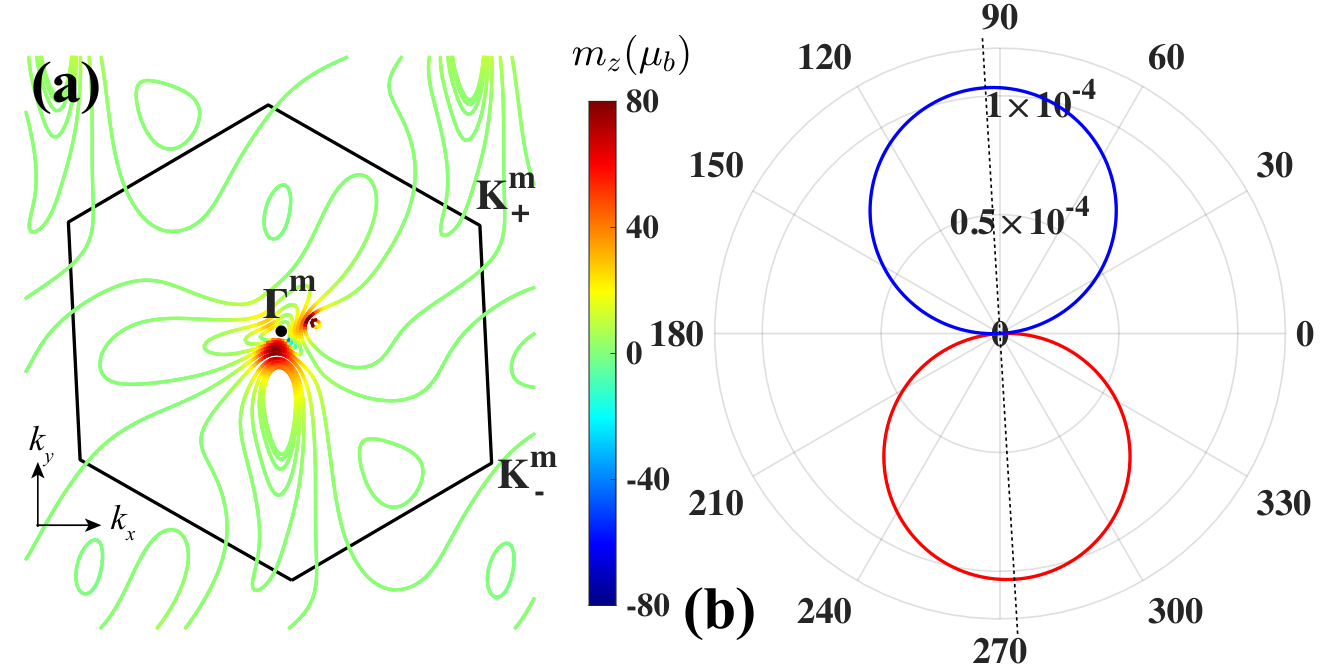
Figure 2: (a) The orbital magnetic moments at different energy contours of the valence band. The tilted hexagon is the mini-Brillouin zone. Here orbital magnetic moment distribution in one valley is shown, and it can be mapped to the case in the other valley through the time reversal symmetry. (b) The out-of-plane orbital magnetization MzM_{z} (in units of μB\mu_{\textrm{B}}/nm2) induced by in-plane current of 1nA/nm along different directions. The optimal direction that generates the largest MzM_{z} is labelled by a black dashed line. The red and blue lines mean positive and negative values of orbital magnetization MzM_{z} respectively. The xx direction has been defined to be along the angular bisector between the two zig-zag directions of the top and bottom graphene layers.

The abrupt change of current-induced magnetization at TcT_{\textrm{c}} in the nonuniform pairing case can be deduced from the Taylor expansion of γi​j\gamma_{ij}, v~i​j\tilde{v}_{ij} in terms of Δν,𝒌\Delta_{\nu,\bm{k}}, which yields γi​j∼eℏ​∑ν∮Mν,𝒌F​vν,𝒌F,j​|Δν,𝒌F|2​d​𝒌F\gamma_{ij}\sim\frac{e}{\hbar}\sum_{\nu}\oint M_{\nu,\bm{k}_{\textrm{F}}}v_{\nu,\bm{k}_{\textrm{F}},j}|\Delta_{\nu,\bm{k}_{\textrm{F}}}|^{2}d\bm{k}_{\textrm{F}} and v~i​j∼e2ℏ2​∑ν∮vν,𝒌F,i​vν,𝒌F,j​|Δν,𝒌F|2​d​𝒌F\tilde{v}_{ij}\sim\frac{e^{2}}{\hbar^{2}}\sum_{\nu}\oint v_{\nu,\bm{k}_{\textrm{F}},i}v_{\nu,\bm{k}_{\textrm{F}},j}|\Delta_{\nu,\bm{k}_{\textrm{F}}}|^{2}d\bm{k}_{\textrm{F}} SM. Above TcT_{\textrm{c}}, we know γi​j∼eℏ​∑ν∮Mν,𝒌F,i​vν,𝒌F,j​d​𝒌F\gamma_{ij}\sim\frac{e}{\hbar}\sum_{\nu}\oint M_{\nu,\bm{k}_{\textrm{F}},i}v_{\nu,\bm{k}_{\textrm{F}},j}d\bm{k}_{\textrm{F}} and v~i​j∼e2ℏ2​∑ν∮vν,𝒌F,i​vν,𝒌F,j​d​𝒌F\tilde{v}_{ij}\sim\frac{e^{2}}{\hbar^{2}}\sum_{\nu}\oint v_{\nu,\bm{k}_{\textrm{F}},i}v_{\nu,\bm{k}_{\textrm{F}},j}d\bm{k}_{\textrm{F}} SM, so the dependence on the paring Δν,𝒌F\Delta_{\nu,\bm{k}_{\textrm{F}}} arises abruptly in the susceptibility αi​j\alpha_{ij} once T<TcT<T_{\textrm{c}}. When the pairing is nonuniform on the Fermi surfaces, the susceptibility αi​j\alpha_{ij} thus differs at the two sides of TcT_{\textrm{c}}. Such abrupt change of current-induced magnetization across TcT_{\textrm{c}} is an indicator of the nonuniform pairing in the superconducting state.

The orbital magnetoelectric effect in superconducting twisted bilayer graphene. In previous studies, current-induced magnetization in the superconducting state only involves the spin magnetization caused by SOC Levitov; Edelstein1; Edelstein2; Yip; Samokhin; Fujimoto; Sigrist; Tkachov; Wenyu1. Recently, superconductivity was observed in TBG which has negligibly small SOC. Here, we predict that a large orbital magnetization can be induced by a current in superconducting TBG. More importantly, the behavior of the current-induced orbital magnetization in TBG near TcT_{\textrm{c}} provides further information about the pairing gap in TBG.

The TBG that shows superconductivity in experiment lies on the hBN substrate, so the coupling of the bottom graphene layer with the hBN can gap out the Dirac points and generate finite Berry curvature MacDonald; Senthil1; Senthil2; Zaletel. Due to the mismatch between the hBN and the bottom graphene layer, the equilateral triangle Moiré superlattice has been observed to get deformed Perge; Pasupathy; Yazdani, indicating that the C3 symmetry of the TBG is generally broken by the strain from the hBN substrate. The resulting TBG system has the lowest C1 symmetry with finite Berry curvature, so an in-plane current can give rise to an out-of-plane orbital magnetization Mz=αz​x​Jx+αz​y​JyM_{z}=\alpha_{zx}J_{x}+\alpha_{zy}J_{y} in the normal state  Wenyu2. Since at the T=0T=0 K the current-induced magnetization in the normal state is the same as the supercurrent-induced magnetization, the current-induced orbital magnetization in TBG is always maintained in its superconducting state. To demonstrate the in-plane current-induced out-of-plane orbital magnetization in a superconducting TBG on hBN, we construct the continuum model for a TBG with a twist angle of 1.6∘1.6^{\circ} Neto1; Neto2; MacDonald2. In the TBG, there is a uniaxial strain applied along the zig-zag direction in the bottom graphene layer to have it stretched by 0.1% (the detailed description for the strained TBG can be found in the Supplemental Material SM). With the massive Dirac gap of 34meV David2; Jung, the Bloch electrons in the valence Moiré flat band carry orbital magnetic moments up to 80 μB\mu_{\textrm{B}} as shown in Fig. 2 (a). Around 1/2 filling in the valence Moiré flat band, the in-plane supercurrent induced out-of-plane orbital magnetization at T=0​KT=0K is directly computed through Eq. 6 and 7. Assuming the in-plane supercurrent density to be 1nA/nm, the out-of-plane orbital magenetization as a function of the in-plane supercurrent direction is shown in Fig. 2 (b). The largest orbital magnetization induced by the in-plane current along the optimal direction reaches the order of 10−4μB/10^{-4}\mu_{\textrm{B}}/nm2. This magnitude of orbital magnetization is comparable to the current induced spin polarization in large Rashba SOC materials under E=103∼104E=10^{3}\sim 10^{4}V/m, such as Au (111) surfaces and Bi/Ag bilayers Johansson1; Johansson2.

Refer to caption
Figure 3: (a) The pairing gap at different energy contours of the valence band. The pairing is plotted in one valley and that in the other valley can be obtained through time reversal symmetry. (b) The current-induced out-of-plane orbital magnetization across the superconductor-normal metal phase transition. The applied in-plane current density is 1nA/nm and the direction is along the optimal direction labelled in Fig. 2 (b). The out-of-plane orbital magnetization exhibits an abrupt jump in nonuniform pairing case while it shows smooth transition across TcT_{\textrm{c}} in uniform paring case.

Near the superconductor-normal metal phase transition, the proportion of orbital magnetization that comes from the quasiparticle current becomes considerable, so the pairing gap that controls the quasiparticle excitations will affect the current-induced orbital magnetization near TcT_{\textrm{c}}. For the superconducting TBG on hBN, a possible nonuniform singlet pairing can be approximated as Δν,𝒌/Δ0=1+λ⁡{cos⁡(𝒌⋅𝒂~1)+cos⁡(𝒌⋅𝒂~2)+cos⁡[𝒌⋅(𝒂~1−𝒂~2)]}\Delta_{\nu,\bm{k}}/\Delta_{0}=1+\lambda\left\{\cos\left(\bm{k}\cdot\tilde{\bm{a}}_{1}\right)+\cos\left(\bm{k}\cdot\tilde{\bm{a}}_{2}\right)+\cos\left[\bm{k}\cdot\left(\tilde{\bm{a}}_{1}-\tilde{\bm{a}}_{2}\right)\right]\right\} BiaoLian; DasSarma; Martin; FengchengWu; Heikkila, with Δ0=1.76​kB​Tc​tanh⁡(1.78​Tc/T−1)\Delta_{0}=1.76k_{\textrm{B}}T_{\textrm{c}}\tanh\left(1.78\sqrt{T_{\textrm{c}}/T-1}\right) and 𝒂~1\tilde{\bm{a}}_{1}, 𝒂~2\tilde{\bm{a}}_{2} being the primitive lattice vectors of the Moiré superlattice under strain SM. The nonuniform pairing gap at λ=0.5\lambda=0.5 is plotted in the mini-Brillouin zone shown in Fig. 3 (a), and the orbital magnetization induced by the current along the optimal direction clearly exhibits an abrupt jump at TcT_{\textrm{c}} as seen in Fig. 3 (b). In contrast, in the uniform pairing case which has λ=0\lambda=0, the current-induced orbital magnetization has smooth connection across TcT_{\textrm{c}}. This is consistent with our analysis that an abrupt change of the current-induced magnetization at TcT_{\textrm{c}} indicates the pairing is nonuniform on the Fermi surfaces.

Discussion. Experimentally, the magnetization that involves orbital magnetic moments polarization in the normal state of materials has been observed through the optical Kerr effect Fai, nuclear magnetic resonance measurements Itou, and the superconducting quantum interference device (SQUID) Young4, and these techniques can all be used to detect the magnetization in the superconducting state JingXia; Curro; Wernsdorfer. In the recent direct image of orbital magnetism in TBG Young4, it can be deduced from the measurement that the surface magnetism at the order of 10−4​μB/nm210^{-4}\mu_{\textrm{B}}/\textrm{nm}^{2} corresponds to the generated static magnetic field around 1nT, so a resolution of 0.1nT SQUID device will be able to detect the orbital magnetization induced by the current density at 1nA/nm in superconducting TBG. The current-induced orbital magnetization and the possible abrupt change at TcT_{\textrm{c}} is proportional to the applied current density in the material, so the critical current density in the superconducting state sets the upper limit of the current-induced orbital magnetization below TcT_{\textrm{c}}. As a result, superconductors with larger pairing gap that have larger critical current density would be preferred to make the effect more measurable.

It is important to note that our theory applies to a large number of recently discovered superconductors with Berry curvatures and negligible SOC, such as a trilayer graphene Moiré superlattice on hBN Fengwang; Kewang; Novoselov; Pablo_Herrero, bilayer graphene/hBN superlattices Taniguchi, and twisted double bilayer graphene Philip; Guangyu. Moreover, our theory also applies to non-centrosymmetric superconductors with strong SOC and finite Berry curvatures such as chiral crystals, Li2Pt3B Salamon, Li2Pd3B Hirata, Mo3Al2C Prozorov, TaRh2B2 and NbRh2B2 Carnicom, which were recently discovered to have superconductivity. In these chiral crystals the orbital magnetic moment carried by the Bloch electrons originates from the Weyl SOC Hasan2, so the spin and orbital magnetization are strongly mixed and the orbital magnetization effect cannot be ignored.

Acknowledgement. The authors would like to thank K. F. Mak for inspiring discussions. K. T. Law acknowledges the support of the Croucher Foundation and HKRGC through C6025-19G, 16310219 and 16309718.

References

  • (1) L. S. Levitov, Yu. V. Nazarov, and G. M. Eliashberg, Magnetostatics of superconductors without an inversion center, JETP Lett. 41, 445 (1985).
  • (2) V. M. Edelstein, Characteristics of the Cooper pairing in two-dimensional noncentrosymmetric electron systems, Sov. Phys. JETP 68, 1244 (1989).
  • (3) V. M. Edelstein, Magnetoelectric Effect in Polar Superconductors, Phys. Rev. Lett. 75, 2004 (1995).
  • (4) S. K. Yip, Two-dimensional superconductivity with strong spin-orbit interaction, Phys. Rev. B 65, 144508 (2002).
  • (5) K. V. Samokhin, Magnetic properties of superconductors with strong spin-orbit coupling, Phys. Rev. B 70, 104521 (2004).
  • (6) S. Fujimoto, Magnetoelectric effects in heavy-fermion superconductors without inversion symmetry, Phys. Rev. B 72, 024515 (2005).
  • (7) E. Bauer and M. Sigrist, Noncentrosymmetric Superconductors (Springer, Berlin, 2012).
  • (8) G. Tkachov, Magnetoelectric Andreev Effect due to Proximity-Induced Nonunitary Triplet Superconductivity in Helical Metals, Phys. Rev. Lett. 118, 016802 (2017).
  • (9) W.-Y. He, and K. T. Law, Magnetoelectric effects in gyrotropic superconductors, Phys. Rev. Research 2, 012073(R) (2020).
  • (10) D. Xiao, M.-C. Chang, and Q. Niu, Berry phase effects on electronic properties, Rev. Mod. Phys. 82, 1959 (2010).
  • (11) Z. Wang, L. Dong, C. Xiao, and Q. Niu, Berry Curvature Effects on Quasiparticle Dynamics in Superconductors, Phys. Rev. Lett. 126, 187001 (2021).
  • (12) M.-C. Chang, and Q. Niu, Berry phase, hyperorbits, and the Hofstadter spectrum: Semiclassical dynamics in magnetic Bloch bands, Phys. Rev. B 53, 7010 (1996).
  • (13) G. Sundaram, and Q. Niu, Wave-packet dynamics in slowly perturbed crystals: Gradient corrections and Berry-phase effects, Phys. Rev. B 59, 14915 (1999).
  • (14) D. Xiao, J. Shi, and Q. Niu, Berry Phase Correction to Electron Density of States in Solids, Phys. Rev. Lett. 95, 137204 (2005).
  • (15) T. Thonhauser, D. Ceresoli, D. Vanderbilt, and R. Resta, Orbital Magnetization in Periodic Insulators, Phys. Rev. Lett. 95, 137205 (2005).
  • (16) D. Ceresoli, T. Thonhauser, D. Vanderbilt, and R. Resta, Orbital magnetization in crystalline solids: Multi-band insulators, Chern insulators, and metals, Phys. Rev. B 74, 024408 (2006).
  • (17) S. Zhong, J. E. Moore, I. Souza, Gyrotropic Magnetic Effect and the Magnetic Moment on the Fermi Surface, Phys. Rev. Lett. 116, 077201 (2016).
  • (18) J. Ma, and D. A. Pesin, Chiral magnetic effect and natural optical activity in metals with or without Weyl points, Phys. Rev. B 92, 235205 (2015).
  • (19) Y. Cao et al., Unconventional superconductivity in magic-angle graphene superlattices, Nature (London) 556, 43 (2018).
  • (20) M. Yankowitz et al., Tuning superconductivity in twisted bilayer graphene, Science 363, 1059 (2019).
  • (21) E. Codecido et al., Correlated insulating and superconducting states in twisted bilayer graphene below the magic angle, Sci. Adv. 5, eaaw9770 (2019).
  • (22) Y. Saito, J. Ge, K. Watanabe, T. Taniguchi, and A. F. Young, Independent superconductors and correlated insulators in twisted bilayer graphene, Nat. Phys. 16, 926 (2020).
  • (23) P. Stepanov et al., Untying the insulating and superconducting orders in magic-angle graphene, Nature 583, 375 (2020).
  • (24) X. Lu et al., Superconductors, orbital magnets and correlated states in magic-angle bilayer graphene, Nature 574, 653 (2019).
  • (25) A. L. Sharpe et al., Emergent ferromagnetism near three-quarters filling in twisted bilayer graphene, Science 365, 605 (2019).
  • (26) M. Serlin et al., Intrinsic quantized anomalous Hall effect in a moiré heterostructure, Science 367, 900 (2019).
  • (27) H. Polshyn et al., H. Polshyn, J. Zhu, M. A. Kumar, Y. Zhang, F. Yang, C. L. Tschirhart, M. Serlin, K. Watanabe, T. Taniguchi, A. H. MacDonald, and A. F. Young, Electrical switching of magnetic order in an orbital Chern insulator, Nature 588, 66 (2020).
  • (28) C. L. Tschirhart et al., Imaging orbital ferromagnetism in a moiré Chern insulator, Science 372, 1323 (2021).
  • (29) See the Supplemental Material for (i) the details about the Bogliubov-de Gennes Hamiltonian in eigenbasis, (ii) the detailed derivation of the current induced magnetization in both the normal metal and superconductivity region, (iii) the continuum model of twisted bilayer graphene on boron nitride with uniaxial strain.
  • (30) A. Ramires, and M. Sigrist, Identifying detrimental effects for multiorbital superconductivity: Application to Sr2RuO4, Phys. Rev. B 94, 104501 (2016).
  • (31) J . R. Schrieffer, Theory of Superconductivity (Avalon Publishing 1999).
  • (32) F. de Juan, A. G. Grushin, T. Morimoto, and J. E. Moore, Quantized circular photogalvanic effect in Weyl semimetals, Nat. Commun. 8, 15995 (2017).
  • (33) M. Xie, and A. H. MacDonald, Nature of the Correlated Insulator States in Twisted Bilayer Graphene, Phys. Rev. Lett. 124, 097601 (2020).
  • (34) Y.-H. Zhang, D. Mao, T. Senthil, Twisted bilayer graphene aligned with hexagonal boron nitride: Anomalous Hall effect and a lattice model, Phys. Rev. Research 1, 033126 (2019).
  • (35) Y.-H. Zhang, D. Mao, Y. Cao, P. Jarillo.-Herrero, and T. Senthil, Nearly flat Chern bands in moiré superlattices, Phys. Rev. B 99, 075127 (2019).
  • (36) N. Bultinck, S. Chatterjee, and M. P. Zaletel, Mechanism for Anomalous Hall Ferromagnetism in Twisted Bilayer Graphene, Phys. Rev. Lett. 124, 166601 (2020).
  • (37) Y. Choi et al., Electronic correlations in twisted bilayer graphene near the magic angle, Nat. Phys. 15, 1174 (2019).
  • (38) A. Kerelsky et al., Maximized electron interactions at the magic angle in twisted bilayer graphene, Nature 572, 95 (2019).
  • (39) Y. Xie et al., Spectroscopic signatures of many-body correlations in magic-angle twisted bilayer graphene, Nature 572, 101 (2019).
  • (40) W.-Y. He, D. G.-Gordon, and K. T. Law, Giant orbital magnetoelectric effect and current-induced magnetization switching in twisted bilayer graphene, Nat. Commun. 11, 1650 (2020).
  • (41) J. M. B. L. Santos, N. M. R. Peres, and A. H. C. Neto, Graphene Bilayer with a Twist: Electronic Structure, Phys. Rev. Lett. 99, 256802 (2007).
  • (42) J. M. B. L. Santos, N. M. R. Peres, and A. H. C. Neto, Continuum model of the twisted graphene bilayer, Phys. Rev. B 86, 155449 (2012).
  • (43) R. Bistritzer, and A. H. MacDonald, Moiré bands in twisted double-layer graphene, Proc. Natl. Acad. Sci. U. S. A. 108, 12233 (2011).
  • (44) M. Lee et al., Ballistic miniband conduction in a graphene superlattice, Science 353, 1526 (2016).
  • (45) H. Kim et al., Accurate Gap Determination in Monolayer and Bilayer Graphene/h-BN Moiré Superlattices, Nano Lett. 18, 7732 (2018).
  • (46) A. Johansson, J. Henk, and I. Mertig, Theoretical aspects of the Edelstein effect for anisotropic two-dimensional electron gas and topological insulators, Phys. Rev. B 93, 195440 (2016).
  • (47) A. Johansson, J. Henk, and I. Mertig, Edelstein effect in Weyl semimetals, Phys. Rev. B 97, 085417 (2018).
  • (48) B. Lian, Z. Wang, and B. A. Bernevig, Twisted Bilayer Graphene: A Phonon-Driven Superconductor, Phys. Rev. Lett. 122, 257002 (2019).
  • (49) F. Wu and S. Das Sarma, Identification of superconducting pairing symmetry in twisted bilayer graphene using in-plane magnetic field and strain, Phys. Rev. B 99, 220507(R) (2019).
  • (50) F. Wu, A. H. MacDonald, and I. Martin, Theory of Phonon-Mediated Superconductivity in Twisted Bilayer Graphene, Phys. Rev. Lett. 121, 257001 (2018).
  • (51) F. Wu, Topological chiral superconductivity with spontaneous vortices and supercurrent in twisted bilayer graphene, Phys. Rev. B 99, 195114 (2019).
  • (52) T. J. Peltonen, R. Ojajarvi, and T. T. Heikkila, Mean-field theory for superconductivity in twisted bilayer graphene, Phys. Rev. B 98, 220504(R) (2018).
  • (53) J. Lee, Z. Wang, H. Xie, K. F. Mak, and J. Shan, Valley magnetoelectricity in single-layer MoS2, Nat. Mater. 16, 887 (2017).
  • (54) T. Furukawa, Y. Shimokawa, K. Kobayashi, and T. Itou, Observation of current-induced bulk magnetization in elemental tellurium, Nat. Commun. 8, 954 (2017).
  • (55) J. Xia, Y. Maeno, P. T. Beyersdorf, M. M. Fejer, and A. Kapitulnik, High Resolution Polar Kerr Effect Measurements of Sr2RuO4: Evidence for Broken Time-Reversal Symmetry in the Superconducting State, Phys. Rev. Lett. 97, 167002 (2006).
  • (56) N. J. Curro, Nuclear magnetic resonance in the heavy fermion superconductors, Rep. Prog. Phys. 72, 026502 (2009).
  • (57) W. Wernsdorfer, From micro- to nano-SQUIDs: applications to nanomagnetism, Supercond. Sci. Technol. 22, 064013 (2009).
  • (58) G. Chen et al., Signatures of tunable superconductivity in a trilayer graphene moiré superlattice, Nature 572, 215 (2019).
  • (59) K.-T. Tsai et al., Correlated Insulating States and Transport Signature of Superconductivity in Twisted Trilayer Graphene Moiré of Moiré Superlattices, arXiv: 1912.03375.
  • (60) S. Xu et al., Tunable van Hove singularities and correlated states in twisted monolayer–bilayer graphene, Nat. Phys. 17 619 (2021).
  • (61) J. M. Park et al., Tunable strongly coupled superconductivity in magic-angle twisted trilayer graphene, Nature 590, 249 (2021).
  • (62) S. Moriyama et al., Observation of superconductivity in bilayer graphene/hexagonal boron nitride superlattices, arXiv: 1901.09356.
  • (63) X. Liu et al., Tunable spin-polarized correlated states in twisted double bilayer graphene, Nature 583, 221 (2020).
  • (64) C. Shen et al., Correlated states in twisted double bilayer graphene, Nat. Phys. 16, 520 (2020).
  • (65) H. Q. Yuan, D. F. Agterberg, N. Hayashi, P. Badica, D. Vandervelde, K. Togano, M. Sigrist, and M. B. Salamon, SS-Wave Spin-Triplet Order in Superconductors without Inversion Symmetry: Li2Pd3B and Li2Pt3B, Phys. Rev. Lett. 97, 017006 (2006).
  • (66) K. Togano, P. Badica, Y. Nakamori, S. Orimo, H. Takeya, and K. Hirata, Superconductivity in the Metal Rich Li-Pd-B Ternary Boride, Phys. Rev. Lett. 93, 247004 (2004).
  • (67) A. B. Karki et al., Structure and physical properties of the noncentrosymmetric superconductor Mo3Al2C, Phys. Rev. B 82, 064512 (2010).
  • (68) E. M. Carnicom et al., TaRh2B2 and NbRh2B2: Superconductors with a chiral noncentrosymmetric crystal structure, Sci. Adv. 4, 7969 (2018).
  • (69) G. Chang et al., Topological quantum properties of chiral crystals, Nat. Mater. 17, 978 (2018).

Supplemental Material for “Superconducting Orbital Magnetoelectric Effect and its Evolution across the Superconductivity Normal Metal Phase Transition”

I Bogliubov-de Gennes Hamiltonian and the Green’s Function

The generic Hamiltonian that can describe the normal state of a system takes the form

ℋ0=∑ν,ν′,𝒌cν,𝒌†​H0,ν​ν′​cν′,𝒌,\displaystyle\mathcal{H}_{0}=\sum_{\nu,\nu^{\prime},\bm{k}}c^{\dagger}_{\nu,\bm{k}}H_{0,\nu\nu^{\prime}}c_{\nu^{\prime},\bm{k}}, (S1)

with cν,𝒌†​(cν,𝒌)c^{\dagger}_{\nu,\bm{k}}\left(c_{\nu,\bm{k}}\right) being the creation (or annihilation) operator, H0,ν​ν′​(𝒌)H_{0,\nu\nu^{\prime}}\left(\bm{k}\right) being the element of the Hamiltonian matrix H0​(𝒌)H_{0}\left(\bm{k}\right), and ν=1,2,3,…\nu=1,2,3,\dots denoting the spin and orbital index of the system. The Bogliubov-de Gennes Hamiltonian that can describe the superconductivity state of a system is

ℋ=12​∑𝒌(c𝒌†c−𝒌)​(H0​(𝒌)Δ^​(𝒌)Δ^†​(𝒌)−H0∗​(−𝒌))​(c𝒌c−𝒌†),\displaystyle\mathcal{H}=\frac{1}{2}\sum_{\bm{k}}\begin{pmatrix}c^{\dagger}_{\bm{k}}&c_{-\bm{k}}\end{pmatrix}\begin{pmatrix}H_{0}\left(\bm{k}\right)&\hat{\Delta}\left(\bm{k}\right)\\ \hat{\Delta}^{\dagger}\left(\bm{k}\right)&-H^{\ast}_{0}\left(-\bm{k}\right)\end{pmatrix}\begin{pmatrix}c_{\bm{k}}\\ c^{\dagger}_{-\bm{k}}\end{pmatrix}, (S2)

where c𝒌=[c1,𝒌,c2,𝒌,c3,𝒌,…]Tc_{\bm{k}}=\left[c_{1,\bm{k}},c_{2,\bm{k}},c_{3,\bm{k}},\dots\right]^{\textrm{T}}, c𝒌†=[c1,𝒌†,c2,𝒌†,c3,𝒌†,…]c^{\dagger}_{\bm{k}}=\left[c^{\dagger}_{1,\bm{k}},c^{\dagger}_{2,\bm{k}},c^{\dagger}_{3,\bm{k}},\dots\right], and Δ^​(𝒌)\hat{\Delta}\left(\bm{k}\right) is the pairing matrix. We know that the normal state Hamiltonian H0​(𝒌)H_{0}\left(\bm{k}\right) can be diagonalized by an unitary transformation U⁡(𝒌)U\left(\bm{k}\right) as

U⁡(𝒌)​H0​(𝒌)​U†​(𝒌)=diag​[ξ1,𝒌,ξ2,𝒌,…,ξν,𝒌],\displaystyle U\left(\bm{k}\right)H_{0}\left(\bm{k}\right)U^{\dagger}\left(\bm{k}\right)=\textrm{diag}\left[\xi_{1,\bm{k}},\xi_{2,\bm{k}},\dots,\xi_{\nu,\bm{k}}\right], (S3)

with U†​(𝒌)​U​(𝒌)=1U^{\dagger}\left(\bm{k}\right)U\left(\bm{k}\right)=1 and the corresponding eigen states ϕν,𝒌=Uν​ν′​(𝒌)​cν′,𝒌\phi_{\nu,\bm{k}}=U_{\nu\nu^{\prime}}\left(\bm{k}\right)c_{\nu^{\prime},\bm{k}}, ϕν,𝒌†=cν′,𝒌†​Uν′​ν∗​(𝒌)\phi^{\dagger}_{\nu,\bm{k}}=c^{\dagger}_{\nu^{\prime},\bm{k}}U^{\ast}_{\nu^{\prime}\nu}\left(\bm{k}\right). Applying the unitary transformation to the Bogliubov-de Gennes Hamiltonian then yields

(U𝒌00U−𝒌∗)​(H0​(𝒌)Δ^𝒌Δ^𝒌†−H0∗​(−𝒌))​(U𝒌†00U−𝒌T)=(U𝒌​H0​(𝒌)​U𝒌†U𝒌​Δ^𝒌​U−𝒌TU−𝒌∗​Δ^𝒌†​U𝒌†−U−𝒌∗​H0∗​(−𝒌)​U−𝒌T).\displaystyle\begin{pmatrix}U_{\bm{k}}&0\\ 0&U^{\ast}_{-\bm{k}}\end{pmatrix}\begin{pmatrix}H_{0}\left(\bm{k}\right)&\hat{\Delta}_{\bm{k}}\\ \hat{\Delta}^{\dagger}_{\bm{k}}&-H^{\ast}_{0}\left(-\bm{k}\right)\end{pmatrix}\begin{pmatrix}U^{\dagger}_{\bm{k}}&0\\ 0&U^{\textrm{T}}_{-\bm{k}}\end{pmatrix}=\begin{pmatrix}U_{\bm{k}}H_{0}\left(\bm{k}\right)U^{\dagger}_{\bm{k}}&U_{\bm{k}}\hat{\Delta}_{\bm{k}}U^{\textrm{T}}_{-\bm{k}}\\ U^{\ast}_{-\bm{k}}\hat{\Delta}^{\dagger}_{\bm{k}}U^{\dagger}_{\bm{k}}&-U^{\ast}_{-\bm{k}}H^{\ast}_{0}\left(-\bm{k}\right)U^{\textrm{T}}_{-\bm{k}}\end{pmatrix}. (S4)

Importantly, after the unitary transformation, we obtain

U𝒌​H0​(𝒌)​U𝒌†=diag​[ξ1,𝒌,ξ2,𝒌,…,ξν,𝒌],−U−𝒌∗​H0∗​(−𝒌)​U−𝒌T=diag​[−ξ1,−𝒌,−ξ2,−𝒌,…,−ξν,−𝒌].\displaystyle U_{\bm{k}}H_{0}\left(\bm{k}\right)U^{\dagger}_{\bm{k}}=\textrm{diag}\left[\xi_{1,\bm{k}},\xi_{2,\bm{k}},...,\xi_{\nu,\bm{k}}\right],\quad\quad\quad-U^{\ast}_{-\bm{k}}H_{0}^{\ast}\left(-\bm{k}\right)U^{\textrm{T}}_{-\bm{k}}=\textrm{diag}\left[-\xi_{1,-\bm{k}},-\xi_{2,-\bm{k}},...,-\xi_{\nu,-\bm{k}}\right]. (S5)

In such eigen-band basis [ϕ1,𝒌†,ϕ2,𝒌†,…,ϕν,𝒌†,ϕ1,−𝒌,ϕ2,−𝒌,…,ϕν,−𝒌]\left[\phi^{\dagger}_{1,\bm{k}},\phi^{\dagger}_{2,\bm{k}},...,\phi^{\dagger}_{\nu,\bm{k}},\phi_{1,-\bm{k}},\phi_{2,-\bm{k}},...,\phi_{\nu,-\bm{k}}\right], the intraband pairing ⟨ϕν,−𝒌​ϕν,𝒌⟩\left\langle\phi_{\nu,-\bm{k}}\phi_{\nu,\bm{k}}\right\rangle gives an energetically favourable pairing phase, while other interband pairing will require extra attractive interaction to overcome the energy (momentum) difference Sigrist. In the energetically favourable pairing phase, the pairing matrix respects H0​(𝒌)​Δ^𝒌−Δ^𝒌​H0∗​(−𝒌)=0H_{0}\left(\bm{k}\right)\hat{\Delta}_{\bm{k}}-\hat{\Delta}_{\bm{k}}H^{\ast}_{0}\left(-\bm{k}\right)=0 Sigrist, and the pairing matrix is therefore diagonalized simultaneously by the unitary transformation as

U𝒌​Δ^𝒌​U−𝒌T=diag​[Δ1,𝒌,Δ2,𝒌,…,Δν,𝒌],U−𝒌∗​Δ^𝒌​U𝒌†=diag​[Δ1,𝒌∗,Δ2,𝒌∗,…,Δν,𝒌∗].\displaystyle U_{\bm{k}}\hat{\Delta}_{\bm{k}}U^{\textrm{T}}_{-\bm{k}}=\textrm{diag}\left[\Delta_{1,\bm{k}},\Delta_{2,\bm{k}},...,\Delta_{\nu,\bm{k}}\right],\quad\quad\quad U^{\ast}_{-\bm{k}}\hat{\Delta}_{\bm{k}}U^{\dagger}_{\bm{k}}=\textrm{diag}\left[\Delta^{\ast}_{1,\bm{k}},\Delta^{\ast}_{2,\bm{k}},...,\Delta^{\ast}_{\nu,\bm{k}}\right]. (S6)

As a result, the Bogliubov-de Gennes Hamiltonian in the eigen-band basis takes the form

(U𝒌00U−𝒌∗)​(H0​(𝒌)Δ^𝒌Δ^𝒌†−H0∗​(−𝒌))​(U𝒌†00U−𝒌T)=(ξ1,𝒌000Δ1,𝒌0000ξ2,𝒌000Δ2,𝒌0000⋱000⋱0000ξν,𝒌000Δν,𝒌Δ1,𝒌∗000−ξ1,−𝒌0000Δ2,𝒌∗000−ξ2,−𝒌0000⋱000⋱0000Δν,𝒌∗000−ξν,−𝒌).\displaystyle\begin{pmatrix}U_{\bm{k}}&0\\ 0&U^{\ast}_{-\bm{k}}\end{pmatrix}\begin{pmatrix}H_{0}\left(\bm{k}\right)&\hat{\Delta}_{\bm{k}}\\ \hat{\Delta}^{\dagger}_{\bm{k}}&-H^{\ast}_{0}\left(-\bm{k}\right)\end{pmatrix}\begin{pmatrix}U^{\dagger}_{\bm{k}}&0\\ 0&U^{\textrm{T}}_{-\bm{k}}\end{pmatrix}=\begin{pmatrix}\xi_{1,\bm{k}}&0&0&0&\Delta_{1,\bm{k}}&0&0&0\\ 0&\xi_{2,\bm{k}}&0&0&0&\Delta_{2,\bm{k}}&0&0\\ 0&0&\ddots&0&0&0&\ddots&0\\ 0&0&0&\xi_{\nu,\bm{k}}&0&0&0&\Delta_{\nu,\bm{k}}\\ \Delta^{\ast}_{1,\bm{k}}&0&0&0&-\xi_{1,-\bm{k}}&0&0&0\\ 0&\Delta^{\ast}_{2,\bm{k}}&0&0&0&-\xi_{2,-\bm{k}}&0&0\\ 0&0&\ddots&0&0&0&\ddots&0\\ 0&0&0&\Delta^{\ast}_{\nu,\bm{k}}&0&0&0&-\xi_{\nu,-\bm{k}}\end{pmatrix}. (S7)

We define the Green’s function for the Bogliubov-de Gennes Hamiltonian as

G0−1​(𝒌,i​ωn)=(i​ωn−H0​(𝒌)−Δ^𝒌−Δ^𝒌i​ωn+H0∗​(−𝒌)),andG0​(𝒌,i​ωn)=(Ge​(𝒌,i​ωn)F⁡(𝒌,i​ωn)F†​(𝒌,i​ωn)Gh​(𝒌,i​ωn))\displaystyle G^{-1}_{0}\left(\bm{k},i\omega_{n}\right)=\begin{pmatrix}i\omega_{n}-H_{0}\left(\bm{k}\right)&-\hat{\Delta}_{\bm{k}}\\ -\hat{\Delta}_{\bm{k}}&i\omega_{n}+H^{\ast}_{0}\left(-\bm{k}\right)\end{pmatrix},\quad\textrm{and}\quad G_{0}\left(\bm{k},i\omega_{n}\right)=\begin{pmatrix}G_{e}\left(\bm{k},i\omega_{n}\right)&F\left(\bm{k},i\omega_{n}\right)\\ F^{\dagger}\left(\bm{k},i\omega_{n}\right)&G_{h}\left(\bm{k},i\omega_{n}\right)\end{pmatrix} (S8)

and then we apply the unitary transformation to the Green’s function:

(U𝒌00U−𝒌∗)​(Ge​(𝒌,i​ωn)F⁡(𝒌,i​ωn)F†​(𝒌,i​ωn)Gh​(𝒌,i​ωn))​(U𝒌†00U−𝒌T)=(U𝒌​Ge​(𝒌,i​ωn)​U𝒌†U𝒌​F​(𝒌,i​ωn)​U−𝒌TU−𝒌∗​F†​(𝒌,i​ωn)​U𝒌†U−𝒌∗​Gh​(𝒌,i​ωn)​U−𝒌T),\displaystyle\begin{pmatrix}U_{\bm{k}}&0\\ 0&U^{\ast}_{-\bm{k}}\end{pmatrix}\begin{pmatrix}G_{e}\left(\bm{k},i\omega_{n}\right)&F\left(\bm{k},i\omega_{n}\right)\\ F^{\dagger}\left(\bm{k},i\omega_{n}\right)&G_{h}\left(\bm{k},i\omega_{n}\right)\end{pmatrix}\begin{pmatrix}U^{\dagger}_{\bm{k}}&0\\ 0&U^{\textrm{T}}_{-\bm{k}}\end{pmatrix}=\begin{pmatrix}U_{\bm{k}}G_{e}\left(\bm{k},i\omega_{n}\right)U^{\dagger}_{\bm{k}}&U_{\bm{k}}F\left(\bm{k},i\omega_{n}\right)U^{\textrm{T}}_{-\bm{k}}\\ U^{\ast}_{-\bm{k}}F^{\dagger}\left(\bm{k},i\omega_{n}\right)U^{\dagger}_{\bm{k}}&U^{\ast}_{-\bm{k}}G_{h}\left(\bm{k},i\omega_{n}\right)U^{\textrm{T}}_{-\bm{k}}\end{pmatrix}, (S9)

which gives

U𝒌​Ge​(𝒌,i​ωn)​U𝒌†\displaystyle U_{\bm{k}}G_{e}\left(\bm{k},i\omega_{n}\right)U^{\dagger}_{\bm{k}} =(−i​ωn+ξ1,𝒌ωn2+ξ1,𝒌2+Δ1,𝒌​Δ1,𝒌∗0000−i​ωn+ξ2,𝒌ωn2+ξ2,𝒌2+Δ2,𝒌​Δ2,𝒌∗0000...0000−i​ωn+ξν,𝒌ωn2+ξν,𝒌2+Δν,𝒌​Δν,𝒌∗),\displaystyle=\begin{pmatrix}-\frac{i\omega_{n}+\xi_{1,\bm{k}}}{\omega_{n}^{2}+\xi^{2}_{1,\bm{k}}+\Delta_{1,\bm{k}}\Delta^{\ast}_{1,\bm{k}}}&0&0&0\\ 0&-\frac{i\omega_{n}+\xi_{2,\bm{k}}}{\omega_{n}^{2}+\xi^{2}_{2,\bm{k}}+\Delta_{2,\bm{k}}\Delta^{\ast}_{2,\bm{k}}}&0&0\\ 0&0&...&0\\ 0&0&0&-\frac{i\omega_{n}+\xi_{\nu,\bm{k}}}{\omega_{n}^{2}+\xi^{2}_{\nu,\bm{k}}+\Delta_{\nu,\bm{k}}\Delta^{\ast}_{\nu,\bm{k}}}\end{pmatrix}, (S10)
U𝒌​F​(𝒌,i​ωn)​U−𝒌T\displaystyle U_{\bm{k}}F\left(\bm{k},i\omega_{n}\right)U^{\textrm{T}}_{-\bm{k}} =(−Δ1,𝒌ωn2+ξ1,𝒌2+Δ1,𝒌​Δ1,𝒌∗0000−Δ2,𝒌ωn2+ξ2,𝒌2+Δ2,𝒌​Δ2,𝒌∗0000...0000−Δν,𝒌ωn2+ξν,𝒌2+Δν,𝒌​Δν,𝒌∗),\displaystyle=\begin{pmatrix}-\frac{\Delta_{1,\bm{k}}}{\omega_{n}^{2}+\xi^{2}_{1,\bm{k}}+\Delta_{1,\bm{k}}\Delta^{\ast}_{1,\bm{k}}}&0&0&0\\ 0&-\frac{\Delta_{2,\bm{k}}}{\omega_{n}^{2}+\xi^{2}_{2,\bm{k}}+\Delta_{2,\bm{k}}\Delta^{\ast}_{2,\bm{k}}}&0&0\\ 0&0&...&0\\ 0&0&0&-\frac{\Delta_{\nu,\bm{k}}}{\omega_{n}^{2}+\xi^{2}_{\nu,\bm{k}}+\Delta_{\nu,\bm{k}}\Delta^{\ast}_{\nu,\bm{k}}}\end{pmatrix}, (S11)
U−𝒌∗​F†​(𝒌,i​ωn)​U𝒌†\displaystyle U^{\ast}_{-\bm{k}}F^{\dagger}\left(\bm{k},i\omega_{n}\right)U^{\dagger}_{\bm{k}} =(−Δ1,𝒌∗ωn2+ξ1,𝒌2+Δ1,𝒌​Δ1,𝒌∗0000−Δ2,𝒌∗ωn2+ξ2,𝒌2+Δ2,𝒌​Δ2,𝒌∗0000...0000−Δν,𝒌∗ωn2+ξν,𝒌2+Δν,𝒌​Δν,𝒌∗),\displaystyle=\begin{pmatrix}-\frac{\Delta^{\ast}_{1,\bm{k}}}{\omega_{n}^{2}+\xi^{2}_{1,\bm{k}}+\Delta_{1,\bm{k}}\Delta^{\ast}_{1,\bm{k}}}&0&0&0\\ 0&-\frac{\Delta^{\ast}_{2,\bm{k}}}{\omega_{n}^{2}+\xi^{2}_{2,\bm{k}}+\Delta_{2,\bm{k}}\Delta^{\ast}_{2,\bm{k}}}&0&0\\ 0&0&...&0\\ 0&0&0&-\frac{\Delta^{\ast}_{\nu,\bm{k}}}{\omega_{n}^{2}+\xi^{2}_{\nu,\bm{k}}+\Delta_{\nu,\bm{k}}\Delta^{\ast}_{\nu,\bm{k}}}\end{pmatrix}, (S12)
U−𝒌∗​Gh​(𝒌,i​ωn)​U−𝒌T\displaystyle U^{\ast}_{-\bm{k}}G_{h}\left(\bm{k},i\omega_{n}\right)U^{\textrm{T}}_{-\bm{k}} =(−i​ωn−ξ1,𝒌ωn2+ξ1,𝒌2+Δ1,𝒌​Δ1,𝒌∗0000−i​ωn−ξ2,𝒌ωn2+ξ2,𝒌2+Δ2,𝒌​Δ2,𝒌∗0000...0000−i​ωn−ξν,𝒌ωn2+ξν,𝒌2+Δν,𝒌​Δν,𝒌∗).\displaystyle=\begin{pmatrix}-\frac{i\omega_{n}-\xi_{1,\bm{k}}}{\omega_{n}^{2}+\xi^{2}_{1,\bm{k}}+\Delta_{1,\bm{k}}\Delta^{\ast}_{1,\bm{k}}}&0&0&0\\ 0&-\frac{i\omega_{n}-\xi_{2,\bm{k}}}{\omega_{n}^{2}+\xi^{2}_{2,\bm{k}}+\Delta_{2,\bm{k}}\Delta^{\ast}_{2,\bm{k}}}&0&0\\ 0&0&...&0\\ 0&0&0&-\frac{i\omega_{n}-\xi_{\nu,\bm{k}}}{\omega_{n}^{2}+\xi^{2}_{\nu,\bm{k}}+\Delta_{\nu,\bm{k}}\Delta^{\ast}_{\nu,\bm{k}}}\end{pmatrix}. (S13)

II Linear Response Theory for the current-induced Magnetization

Applying current introduces a perturbation

δ​ℋ=\displaystyle\delta\mathcal{H}= −∑𝒌,𝒒c𝒌−12​𝒒†c𝒌+12​𝒒[eℏ∂kiH0(𝒌)Ai(−𝒒,t)−e22​ℏ2∂ki​kj2H0(𝒌)Ai(𝒒,t)Aj(−𝒒,t)]\displaystyle-\sum_{\bm{k},\bm{q}}c^{\dagger}_{\bm{k}-\frac{1}{2}\bm{q}}c_{\bm{k}+\frac{1}{2}\bm{q}}\left[\frac{e}{\hbar}\partial_{k_{i}}H_{0}\left(\bm{k}\right)A_{i}\left(-\bm{q},t\right)-\frac{e^{2}}{2\hbar^{2}}\partial^{2}_{k_{i}k_{j}}H_{0}\left(\bm{k}\right)A_{i}\left(\bm{q},t\right)A_{j}\left(-\bm{q},t\right)\right] (S14)

to the Bogliubov-de Gennes Hamiltonian, so the free-energy density of the system gets changed. The change of free-energy density can be obtained through expanding the electromagnetic gauge fields, and it can be expressed as

Δ​F=\displaystyle\Delta F= 12​∑𝒒,mAi​(−𝒒,−i​ωm)​Πi​j​(𝒒,i​ωm)​Aj​(𝒒,i​ωm)\displaystyle\frac{1}{2}\sum_{\bm{q},m}A_{i}\left(-\bm{q},-i\omega_{m}\right)\Pi_{ij}\left(\bm{q},i\omega_{m}\right)A_{j}\left(\bm{q},i\omega_{m}\right)
+12∑𝒒,mBi(−𝒒,−iωm)Ti​js(𝒒,iωm)Aj(𝒒,iωm)+12∑𝒒,mAi(−𝒒,−iωm)T~i​js(𝒒,iωm)Bj(𝒒,iωm).\displaystyle+\frac{1}{2}\sum_{\bm{q},m}B_{i}\left(-\bm{q},-i\omega_{m}\right)T^{\textrm{s}}_{ij}\left(\bm{q},i\omega_{m}\right)A_{j}\left(\bm{q},i\omega_{m}\right)+\frac{1}{2}\sum_{\bm{q},m}A_{i}\left(-\bm{q},-i\omega_{m}\right)\tilde{T}_{ij}^{\textrm{s}}\left(\bm{q},i\omega_{m}\right)B_{j}\left(\bm{q},i\omega_{m}\right). (S15)

Here, the terms Ti​js​(𝒒,i​ωm)T^{\textrm{s}}_{ij}\left(\bm{q},i\omega_{m}\right) and T~i​js​(𝒒,i​ωm)\tilde{T}^{\textrm{s}}_{ij}\left(\bm{q},i\omega_{m}\right), where

Ti​js​(𝒒,i​ωm)=\displaystyle T_{ij}^{\textrm{s}}\left(\bm{q},i\omega_{m}\right)= 1β​V∑𝒌,ntr[Ge(𝒌−12𝒒,iωn)12μBgσiGe(𝒌+12𝒒,iωn+iωm)eℏ∂H0​(𝒌)∂kj\displaystyle\frac{1}{\beta V}\sum_{\bm{k},n}\textrm{tr}\left[G_{e}\left(\bm{k}-\frac{1}{2}\bm{q},i\omega_{n}\right)\frac{1}{2}\mu_{\textrm{B}}g\sigma_{i}G_{e}\left(\bm{k}+\frac{1}{2}\bm{q},i\omega_{n}+i\omega_{m}\right)\frac{e}{\hbar}\frac{\partial H_{0}\left(\bm{k}\right)}{\partial k_{j}}\right.
−F(𝒌−12𝒒,iωn)12μBgσi∗F†(𝒌+12𝒒,iωn+iωm)eℏ∂H0​(𝒌)∂kj],\displaystyle\left.-F\left(\bm{k}-\frac{1}{2}\bm{q},i\omega_{n}\right)\frac{1}{2}\mu_{\textrm{B}}g\sigma_{i}^{\ast}F^{\dagger}\left(\bm{k}+\frac{1}{2}\bm{q},i\omega_{n}+i\omega_{m}\right)\frac{e}{\hbar}\frac{\partial H_{0}\left(\bm{k}\right)}{\partial k_{j}}\right], (S16)
T~i​js​(𝒒,i​ωm)=\displaystyle\tilde{T}_{ij}^{\textrm{s}}\left(\bm{q},i\omega_{m}\right)= 1β​V∑𝒌,ntr[Ge(𝒌−12𝒒,iωn)eℏ∂H0​(𝒌)∂kiGe(𝒌+12𝒒,iωn+iωm)12μBgσj\displaystyle\frac{1}{\beta V}\sum_{\bm{k},n}\textrm{tr}\left[G_{e}\left(\bm{k}-\frac{1}{2}\bm{q},i\omega_{n}\right)\frac{e}{\hbar}\frac{\partial H_{0}\left(\bm{k}\right)}{\partial k_{i}}G_{e}\left(\bm{k}+\frac{1}{2}\bm{q},i\omega_{n}+i\omega_{m}\right)\frac{1}{2}\mu_{\textrm{B}}g\sigma_{j}\right.
−F(𝒌−12𝒒,iωn)eℏ∂H0∗​(−𝒌)−∂kiF0†(𝒌+12𝒒,iωn+iωm)12μBgσj].\displaystyle\left.-F\left(\bm{k}-\frac{1}{2}\bm{q},i\omega_{n}\right)\frac{e}{\hbar}\frac{\partial H^{\ast}_{0}\left(-\bm{k}\right)}{-\partial k_{i}}F^{\dagger}_{0}\left(\bm{k}+\frac{1}{2}\bm{q},i\omega_{n}+i\omega_{m}\right)\frac{1}{2}\mu_{\textrm{B}}g\sigma_{j}\right]. (S17)

give the spin magnetoelectric susceptibility in both the superconductivity and normal metal regions, while the polarization tensor Πi​j​(𝒒,i​ωm)\Pi_{ij}\left(\bm{q},i\omega_{m}\right), where

Πi​j​(𝒒,i​ωm)=\displaystyle\Pi_{ij}\left(\bm{q},i\omega_{m}\right)= 1β​V∑𝒌,ntr[Ge(𝒌,iωn)e2ℏ2∂2H0​(𝒌)∂ki​∂kj+Ge(𝒌−12𝒒,iωn)eℏ∂H0​(𝒌)∂kiGe(𝒌+12𝒒,iωn+iωm)eℏ∂H0​(𝒌)∂kj\displaystyle\frac{1}{\beta V}\sum_{\bm{k},n}\textrm{tr}\left[G_{e}\left(\bm{k},i\omega_{n}\right)\frac{e^{2}}{\hbar^{2}}\frac{\partial^{2}H_{0}\left(\bm{k}\right)}{\partial k_{i}\partial k_{j}}+G_{e}\left(\bm{k}-\frac{1}{2}\bm{q},i\omega_{n}\right)\frac{e}{\hbar}\frac{\partial H_{0}\left(\bm{k}\right)}{\partial k_{i}}G_{e}\left(\bm{k}+\frac{1}{2}\bm{q},i\omega_{n}+i\omega_{m}\right)\frac{e}{\hbar}\frac{\partial H_{0}\left(\bm{k}\right)}{\partial k_{j}}\right.
+F(𝒌−12𝒒,iωn)eℏ∂H0∗​(−𝒌)∂kiF†(𝒌+12𝒒,iωn+iωm)eℏ∂H0​(𝒌)∂kj],\displaystyle\left.+F\left(\bm{k}-\frac{1}{2}\bm{q},i\omega_{n}\right)\frac{e}{\hbar}\frac{\partial H^{\ast}_{0}\left(-\bm{k}\right)}{\partial k_{i}}F^{\dagger}\left(\bm{k}+\frac{1}{2}\bm{q},i\omega_{n}+i\omega_{m}\right)\frac{e}{\hbar}\frac{\partial H_{0}\left(\bm{k}\right)}{\partial k_{j}}\right], (S18)

is responsible for the current and current-induced orbital magnetization in both the superconductivity and normal metal regions.

II.1 Polarization Tensor, Current, and the Current-induced Orbital Magnetization

Substituting Eq. S10, S11, S12, S13 into Eq. II, we can obtain the polarization tensor Πi​j​(𝒒,i​ωm)\Pi_{ij}\left(\bm{q},i\omega_{m}\right), where

Πi​j​(𝒒,i​ωm)=Πi​jsta​(𝒒)+Πi​jdyn​(𝒒,i​ωm),\displaystyle\Pi_{ij}\left(\bm{q},i\omega_{m}\right)=\Pi_{ij}^{\textrm{sta}}\left(\bm{q}\right)+\Pi_{ij}^{\textrm{dyn}}\left(\bm{q},i\omega_{m}\right),

with the static part Πi​jsta​(𝒒)\Pi^{\textrm{sta}}_{ij}\left(\bm{q}\right)

Πi​jsta​(𝒒)=\displaystyle\Pi^{\textrm{sta}}_{ij}\left(\bm{q}\right)= 12​V​e2ℏ2​∑𝒌,ν[ϵν,𝒌+ξν,𝒌ϵν,𝒌​f​(ϵν,𝒌)+ϵν,𝒌−ξν,𝒌ϵν,𝒌​f​(−ϵν,𝒌)]​⟨ϕν,𝒌|​∂ki​kj2H0​(𝒌)​|ϕν,𝒌⟩\displaystyle\frac{1}{2V}\frac{e^{2}}{\hbar^{2}}\sum_{\bm{k},\nu}\left[\frac{\epsilon_{\nu,\bm{k}}+\xi_{\nu,\bm{k}}}{\epsilon_{\nu,\bm{k}}}f\left(\epsilon_{\nu,\bm{k}}\right)+\frac{\epsilon_{\nu,\bm{k}}-\xi_{\nu,\bm{k}}}{\epsilon_{\nu,\bm{k}}}f\left(-\epsilon_{\nu,\bm{k}}\right)\right]\bra{\phi_{\nu,\bm{k}}}\partial^{2}_{k_{i}k_{j}}H_{0}\left(\bm{k}\right)\ket{\phi_{\nu,\bm{k}}}
−12​Ve2ℏ2∑𝒌,ν,ν′[(1−ξν,𝒌−12​𝒒​ξν′,𝒌+12​𝒒+Δν,𝒌−12​𝒒​Δν′,𝒌+12​𝒒∗ϵν′,𝒌+12​𝒒​ϵν,𝒌−12​𝒒)1−f⁡(ϵν′,𝒌+12​𝒒)−f⁡(ϵν,𝒌−12​𝒒)ϵν′,𝒌+12​𝒒+ϵν,𝒌−12​𝒒\displaystyle-\frac{1}{2V}\frac{e^{2}}{\hbar^{2}}\sum_{\bm{k},\nu,\nu^{\prime}}\left[\left(1-\frac{\xi_{\nu,\bm{k}-\frac{1}{2}\bm{q}}\xi_{\nu^{\prime},\bm{k}+\frac{1}{2}\bm{q}}+\Delta_{\nu,\bm{k}-\frac{1}{2}\bm{q}}\Delta^{\ast}_{\nu^{\prime},\bm{k}+\frac{1}{2}\bm{q}}}{\epsilon_{\nu^{\prime},\bm{k}+\frac{1}{2}\bm{q}}\epsilon_{\nu,\bm{k}-\frac{1}{2}\bm{q}}}\right)\frac{1-f\left(\epsilon_{\nu^{\prime},\bm{k}+\frac{1}{2}\bm{q}}\right)-f\left(\epsilon_{\nu,\bm{k}-\frac{1}{2}\bm{q}}\right)}{\epsilon_{\nu^{\prime},\bm{k}+\frac{1}{2}\bm{q}}+\epsilon_{\nu,\bm{k}-\frac{1}{2}\bm{q}}}\right.
−(1+ξν,𝒌−12​𝒒​ξν′,𝒌+12​𝒒+Δν,𝒌−12​𝒒​Δ𝒌+12​𝒒∗ϵν′,𝒌+12​𝒒​ϵν,𝒌−12​𝒒)f⁡(ϵν′,𝒌+12​𝒒)−f⁡(ϵν,𝒌−12​𝒒)ϵν′,𝒌+12​𝒒−ϵν,𝒌−12​𝒒]\displaystyle\left.-\left(1+\frac{\xi_{\nu,\bm{k}-\frac{1}{2}\bm{q}}\xi_{\nu^{\prime},\bm{k}+\frac{1}{2}\bm{q}}+\Delta_{\nu,\bm{k}-\frac{1}{2}\bm{q}}\Delta^{\ast}_{\bm{k}+\frac{1}{2}\bm{q}}}{\epsilon_{\nu^{\prime},\bm{k}+\frac{1}{2}\bm{q}}\epsilon_{\nu,\bm{k}-\frac{1}{2}\bm{q}}}\right)\frac{f\left(\epsilon_{\nu^{\prime},\bm{k}+\frac{1}{2}\bm{q}}\right)-f\left(\epsilon_{\nu,\bm{k}-\frac{1}{2}\bm{q}}\right)}{\epsilon_{\nu^{\prime},\bm{k}+\frac{1}{2}\bm{q}}-\epsilon_{\nu,\bm{k}-\frac{1}{2}\bm{q}}}\right]
⟨ϕν,𝒌−12​𝒒|​∂kiH0​(𝒌)​|ϕν′,𝒌+12​𝒒⟩​⟨ϕν′,𝒌+12​𝒒|​∂kjH0​(𝒌)​|ϕν,𝒌−12​𝒒⟩,\displaystyle\bra{\phi_{\nu,\bm{k}-\frac{1}{2}\bm{q}}}\partial_{k_{i}}H_{0}\left(\bm{k}\right)\ket{\phi_{\nu^{\prime},\bm{k}+\frac{1}{2}\bm{q}}}\bra{\phi_{\nu^{\prime},\bm{k}+\frac{1}{2}\bm{q}}}\partial_{k_{j}}H_{0}\left(\bm{k}\right)\ket{\phi_{\nu,\bm{k}-\frac{1}{2}\bm{q}}}, (S19)

and the dynamic part Πi​jdyn​(𝒒,i​ωm)\Pi^{\textrm{dyn}}_{ij}\left(\bm{q},i\omega_{m}\right), where

Πi​jdyn​(𝒒,i​ωm)=\displaystyle\Pi_{ij}^{\textrm{dyn}}\left(\bm{q},i\omega_{m}\right)= 14​V∑𝒌,ν,ν′{(1−ξν,𝒌−12​𝒒​ξν′,𝒌+12​𝒒+Δν,𝒌−12​𝒒​Δν′,𝒌+12​𝒒∗ϵν′,𝒌+12​𝒒​ϵν,𝒌−12​𝒒)[i​ωmi​ωm+ϵν′,𝒌+12​𝒒+ϵν,𝒌−12​𝒒+i​ωmi​ωm−(ϵν′,𝒌+12​𝒒+ϵν,𝒌−12​𝒒)]\displaystyle\frac{1}{4V}\sum_{\bm{k},\nu,\nu^{\prime}}\left\{\left(1-\frac{\xi_{\nu,\bm{k}-\frac{1}{2}\bm{q}}\xi_{\nu^{\prime},\bm{k}+\frac{1}{2}\bm{q}}+\Delta_{\nu,\bm{k}-\frac{1}{2}\bm{q}}\Delta^{\ast}_{\nu^{\prime},\bm{k}+\frac{1}{2}\bm{q}}}{\epsilon_{\nu^{\prime},\bm{k}+\frac{1}{2}\bm{q}}\epsilon_{\nu,\bm{k}-\frac{1}{2}\bm{q}}}\right)\left[\frac{i\omega_{m}}{i\omega_{m}+\epsilon_{\nu^{\prime},\bm{k}+\frac{1}{2}\bm{q}}+\epsilon_{\nu,\bm{k}-\frac{1}{2}\bm{q}}}+\frac{i\omega_{m}}{i\omega_{m}-\left(\epsilon_{\nu^{\prime},\bm{k}+\frac{1}{2}\bm{q}}+\epsilon_{\nu,\bm{k}-\frac{1}{2}\bm{q}}\right)}\right]\right.
1−f⁡(ϵν′,𝒌+12​𝒒)−f⁡(ϵν,𝒌−12​𝒒)ϵν′,𝒌+12​𝒒+ϵν,𝒌−12​𝒒\displaystyle\left.\frac{1-f\left(\epsilon_{\nu^{\prime},\bm{k}+\frac{1}{2}\bm{q}}\right)-f\left(\epsilon_{\nu,\bm{k}-\frac{1}{2}\bm{q}}\right)}{\epsilon_{\nu^{\prime},\bm{k}+\frac{1}{2}\bm{q}}+\epsilon_{\nu,\bm{k}-\frac{1}{2}\bm{q}}}\right.
−(1+ξν,𝒌−12​𝒒​ξν′,𝒌+12​𝒒+Δν,𝒌−12​𝒒​Δν′,𝒌+12​𝒒∗ϵν′,𝒌+12​𝒒​ϵν,𝒌−12​𝒒)​[i​ωmi​ωm−(ϵν′,𝒌+12​𝒒−ϵν,𝒌−12​𝒒)+i​ωmi​ωm+ϵν′,𝒌+12​𝒒−ϵν,𝒌−12​𝒒]\displaystyle\left.-\left(1+\frac{\xi_{\nu,\bm{k}-\frac{1}{2}\bm{q}}\xi_{\nu^{\prime},\bm{k}+\frac{1}{2}\bm{q}}+\Delta_{\nu,\bm{k}-\frac{1}{2}\bm{q}}\Delta^{\ast}_{\nu^{\prime},\bm{k}+\frac{1}{2}\bm{q}}}{\epsilon_{\nu^{\prime},\bm{k}+\frac{1}{2}\bm{q}}\epsilon_{\nu,\bm{k}-\frac{1}{2}\bm{q}}}\right)\left[\frac{i\omega_{m}}{i\omega_{m}-\left(\epsilon_{\nu^{\prime},\bm{k}+\frac{1}{2}\bm{q}}-\epsilon_{\nu,\bm{k}-\frac{1}{2}\bm{q}}\right)}+\frac{i\omega_{m}}{i\omega_{m}+\epsilon_{\nu^{\prime},\bm{k}+\frac{1}{2}\bm{q}}-\epsilon_{\nu,\bm{k}-\frac{1}{2}\bm{q}}}\right]\right.
f⁡(ϵν′,𝒌+12​𝒒)−f⁡(ϵν,𝒌−12​𝒒)ϵν′,𝒌+12​𝒒−ϵν,𝒌−12​𝒒}⟨ϕν,𝒌−12​𝒒|eℏ∂kiH0(𝒌)|ϕν′,𝒌+12​𝒒⟩⟨ϕν′,𝒌+12​𝒒|eℏ∂kjH0(𝒌)|ϕν,𝒌−12​𝒒⟩.\displaystyle\left.\frac{f\left(\epsilon_{\nu^{\prime},\bm{k}+\frac{1}{2}\bm{q}}\right)-f\left(\epsilon_{\nu,\bm{k}-\frac{1}{2}\bm{q}}\right)}{\epsilon_{\nu^{\prime},\bm{k}+\frac{1}{2}\bm{q}}-\epsilon_{\nu,\bm{k}-\frac{1}{2}\bm{q}}}\right\}\bra{\phi_{\nu,\bm{k}-\frac{1}{2}\bm{q}}}\frac{e}{\hbar}\partial_{k_{i}}H_{0}\left(\bm{k}\right)\ket{\phi_{\nu^{\prime},\bm{k}+\frac{1}{2}\bm{q}}}\bra{\phi_{\nu^{\prime},\bm{k}+\frac{1}{2}\bm{q}}}\frac{e}{\hbar}\partial_{k_{j}}H_{0}\left(\bm{k}\right)\ket{\phi_{\nu,\bm{k}-\frac{1}{2}\bm{q}}}. (S20)

The static and dynamic part of the polarization tensor can then be expanded in terms of 𝒒\bm{q} to the linear order as

Πi​jsta​(𝒒)=\displaystyle\Pi_{ij}^{\textrm{sta}}\left(\bm{q}\right)= Πi​jsta,(0)+Qi​j​lsta​ql+𝒪⁡(𝒒2),Πi​jdyn​(𝒒,i​ωm)=Πi​jdyn,(0)+Qi​j​ldyn​ql+𝒪⁡(𝒒2),\displaystyle\Pi_{ij}^{\textrm{sta},\left(0\right)}+Q^{\textrm{sta}}_{ijl}q_{l}+\mathcal{O}\left(\bm{q}^{2}\right),\quad\Pi_{ij}^{\textrm{dyn}}\left(\bm{q},i\omega_{m}\right)=\Pi_{ij}^{\textrm{dyn},\left(0\right)}+Q^{\textrm{dyn}}_{ijl}q_{l}+\mathcal{O}\left(\bm{q}^{2}\right), (S21)

with

Qi​j​lsta=lim𝒒→0Πi​jsta​(𝒒)−Πi​jsta​(0)ql,Qi​j​ldyn=lim𝒒→0Πi​jdyn​(𝒒)−Πi​jdyn​(0)ql.\displaystyle Q^{\textrm{sta}}_{ijl}=\lim_{\bm{q}\rightarrow 0}\frac{\Pi^{\textrm{sta}}_{ij}\left(\bm{q}\right)-\Pi^{\textrm{sta}}_{ij}\left(0\right)}{q_{l}},\quad Q^{\textrm{dyn}}_{ijl}=\lim_{\bm{q}\rightarrow 0}\frac{\Pi^{\textrm{dyn}}_{ij}\left(\bm{q}\right)-\Pi^{\textrm{dyn}}_{ij}\left(0\right)}{q_{l}}. (S22)

The intra-band contribution to Πi​jsta,(0)\Pi_{ij}^{\textrm{sta},\left(0\right)} is

Πi​jsta,(0),intra=\displaystyle\Pi^{\textrm{sta},\left(0\right),\textrm{intra}}_{ij}= 12​V​e2ℏ2​∑𝒌,ν⟨ϕν,𝒌|​∂ki​kj2H0​(𝒌)​[ϵν,𝒌+ξν,𝒌ϵν,𝒌​f​(ϵν,𝒌)+ϵν,𝒌−ξν,𝒌ϵν,𝒌​f​(−ϵν,𝒌)]\displaystyle\frac{1}{2V}\frac{e^{2}}{\hbar^{2}}\sum_{\bm{k},\nu}\bra{\phi_{\nu,\bm{k}}}\partial^{2}_{k_{i}k_{j}}H_{0}\left(\bm{k}\right)\left[\frac{\epsilon_{\nu,\bm{k}}+\xi_{\nu,\bm{k}}}{\epsilon_{\nu,\bm{k}}}f\left(\epsilon_{\nu,\bm{k}}\right)+\frac{\epsilon_{\nu,\bm{k}}-\xi_{\nu,\bm{k}}}{\epsilon_{\nu,\bm{k}}}f\left(-\epsilon_{\nu,\bm{k}}\right)\right]
+1Ve2ℏ2∑𝒌,ν⟨ϕν,𝒌|∂kiH0(𝒌)|ϕν,𝒌⟩⟨ϕν,𝒌|∂kjH0(𝒌)|ϕν,𝒌⟩d​f​(ϵν,𝒌)d​ϵν,𝒌\displaystyle+\frac{1}{V}\frac{e^{2}}{\hbar^{2}}\sum_{\bm{k},\nu}\bra{\phi_{\nu,\bm{k}}}\partial_{k_{i}}H_{0}\left(\bm{k}\right)\ket{\phi_{\nu,\bm{k}}}\bra{\phi_{\nu,\bm{k}}}\partial_{k_{j}}H_{0}\left(\bm{k}\right)\ket{\phi_{\nu,\bm{k}}}\frac{df\left(\epsilon_{\nu,\bm{k}}\right)}{d\epsilon_{\nu,\bm{k}}}
≈1V​e2ℏ2​∑𝒌,ν[⟨ϕν,𝒌|​∂ki​kj2H0​(𝒌)​|ϕν,𝒌⟩​f​(ξν,𝒌)+⟨ϕν,𝒌|​∂kiH0​(𝒌)​|ϕν,𝒌⟩​⟨ϕν,𝒌|​∂kjH0​(𝒌)​|ϕν,𝒌⟩​d​f​(ϵν,𝒌)d​ϵν,𝒌].\displaystyle\approx\frac{1}{V}\frac{e^{2}}{\hbar^{2}}\sum_{\bm{k},\nu}\left[\bra{\phi_{\nu,\bm{k}}}\partial^{2}_{k_{i}k_{j}}H_{0}\left(\bm{k}\right)\ket{\phi_{\nu,\bm{k}}}f\left(\xi_{\nu,\bm{k}}\right)+\bra{\phi_{\nu,\bm{k}}}\partial_{k_{i}}H_{0}\left(\bm{k}\right)\ket{\phi_{\nu,\bm{k}}}\bra{\phi_{\nu,\bm{k}}}\partial_{k_{j}}H_{0}\left(\bm{k}\right)\ket{\phi_{\nu,\bm{k}}}\frac{df\left(\epsilon_{\nu,\bm{k}}\right)}{d\epsilon_{\nu,\bm{k}}}\right].

For the inter-band contribution, we assume that the pairing gap |Δν,𝒌||\Delta_{\nu,\bm{k}}| is much smaller than the inversion symmetry breaking-induced band splitting, so the inter-band term can be approximated by that used in the normal metal phase with Δν,𝒌=0\Delta_{\nu,\bm{k}}=0:

Πi​jsta,(0),inter=\displaystyle\Pi^{\textrm{sta},\left(0\right),\textrm{inter}}_{ij}= −12​Ve2ℏ2∑𝒌,ν≠ν′[(1−ξν,𝒌​ξν′,𝒌+Δν,𝒌​Δν′,𝒌∗ϵν′,𝒌​ϵν,𝒌)1−f⁡(ϵν′,𝒌)−f⁡(ϵν,𝒌)ϵν′,𝒌+ϵν,𝒌\displaystyle-\frac{1}{2V}\frac{e^{2}}{\hbar^{2}}\sum_{\bm{k},\nu\neq\nu^{\prime}}\left[\left(1-\frac{\xi_{\nu,\bm{k}}\xi_{\nu^{\prime},\bm{k}}+\Delta_{\nu,\bm{k}}\Delta^{\ast}_{\nu^{\prime},\bm{k}}}{\epsilon_{\nu^{\prime},\bm{k}}\epsilon_{\nu,\bm{k}}}\right)\frac{1-f\left(\epsilon_{\nu^{\prime},\bm{k}}\right)-f\left(\epsilon_{\nu,\bm{k}}\right)}{\epsilon_{\nu^{\prime},\bm{k}}+\epsilon_{\nu,\bm{k}}}\right.
−(1+ξν,𝒌​ξν′,𝒌+Δν,𝒌​Δ𝒌∗ϵν′,𝒌​ϵν,𝒌)f⁡(ϵν′,𝒌)−f⁡(ϵν,𝒌)ϵν′,𝒌−ϵν,𝒌]⟨ϕν,𝒌|∂kiH0(𝒌)|ϕν′,𝒌⟩⟨ϕν′,𝒌|∂kjH0(𝒌)|ϕν,𝒌⟩\displaystyle\left.-\left(1+\frac{\xi_{\nu,\bm{k}}\xi_{\nu^{\prime},\bm{k}}+\Delta_{\nu,\bm{k}}\Delta^{\ast}_{\bm{k}}}{\epsilon_{\nu^{\prime},\bm{k}}\epsilon_{\nu,\bm{k}}}\right)\frac{f\left(\epsilon_{\nu^{\prime},\bm{k}}\right)-f\left(\epsilon_{\nu,\bm{k}}\right)}{\epsilon_{\nu^{\prime},\bm{k}}-\epsilon_{\nu,\bm{k}}}\right]\bra{\phi_{\nu,\bm{k}}}\partial_{k_{i}}H_{0}\left(\bm{k}\right)\ket{\phi_{\nu^{\prime},\bm{k}}}\bra{\phi_{\nu^{\prime},\bm{k}}}\partial_{k_{j}}H_{0}\left(\bm{k}\right)\ket{\phi_{\nu,\bm{k}}}
≈\displaystyle\approx 1V​e2ℏ2​∑𝒌,ν≠ν′f⁡(ξν′,𝒌)−f⁡(ξν,𝒌)ξν′,𝒌−ξν,𝒌​⟨ϕν,𝒌|​∂kiH0​(𝒌)​|ϕν′,𝒌⟩​⟨ϕν′,𝒌|​∂kjH0​(𝒌)​|ϕν,𝒌⟩.\displaystyle\frac{1}{V}\frac{e^{2}}{\hbar^{2}}\sum_{\bm{k},\nu\neq\nu^{\prime}}\frac{f\left(\xi_{\nu^{\prime},\bm{k}}\right)-f\left(\xi_{\nu,\bm{k}}\right)}{\xi_{\nu^{\prime},\bm{k}}-\xi_{\nu,\bm{k}}}\bra{\phi_{\nu,\bm{k}}}\partial_{k_{i}}H_{0}\left(\bm{k}\right)\ket{\phi_{\nu^{\prime},\bm{k}}}\bra{\phi_{\nu^{\prime},\bm{k}}}\partial_{k_{j}}H_{0}\left(\bm{k}\right)\ket{\phi_{\nu,\bm{k}}}. (S23)

We also know from the gauge invariance that

1V​e2ℏ2​∑𝒌,ν≠ν′f⁡(ξν′,𝒌)−f⁡(ξν,𝒌)ξν′,𝒌−ξν,𝒌​⟨ϕν,𝒌|​∂kiH0​(𝒌)​|ϕν′,𝒌⟩​⟨ϕν′,𝒌|​∂kjH0​(𝒌)​|ϕν,𝒌⟩\displaystyle\frac{1}{V}\frac{e^{2}}{\hbar^{2}}\sum_{\bm{k},\nu\neq\nu^{\prime}}\frac{f\left(\xi_{\nu^{\prime},\bm{k}}\right)-f\left(\xi_{\nu,\bm{k}}\right)}{\xi_{\nu^{\prime},\bm{k}}-\xi_{\nu,\bm{k}}}\bra{\phi_{\nu,\bm{k}}}\partial_{k_{i}}H_{0}\left(\bm{k}\right)\ket{\phi_{\nu^{\prime},\bm{k}}}\bra{\phi_{\nu^{\prime},\bm{k}}}\partial_{k_{j}}H_{0}\left(\bm{k}\right)\ket{\phi_{\nu,\bm{k}}}
=\displaystyle= −1Ve2ℏ2∑𝒌,ν[⟨ϕν,𝒌|∂kiH0(𝒌)|ϕν,𝒌⟩⟨ϕν,𝒌|∂kjH0(𝒌)|ϕν,𝒌⟩d​f​(ξν,𝒌)d​ξν,𝒌+⟨ϕν,𝒌|∂ki​kj2H0(𝒌)|ϕν,𝒌⟩f(ξν,𝒌)],\displaystyle-\frac{1}{V}\frac{e^{2}}{\hbar^{2}}\sum_{\bm{k},\nu}\left[\bra{\phi_{\nu,\bm{k}}}\partial_{k_{i}}H_{0}\left(\bm{k}\right)\ket{\phi_{\nu,\bm{k}}}\bra{\phi_{\nu,\bm{k}}}\partial_{k_{j}}H_{0}\left(\bm{k}\right)\ket{\phi_{\nu,\bm{k}}}\frac{df\left(\xi_{\nu,\bm{k}}\right)}{d\xi_{\nu,\bm{k}}}+\bra{\phi_{\nu,\bm{k}}}\partial^{2}_{k_{i}k_{j}}H_{0}\left(\bm{k}\right)\ket{\phi_{\nu,\bm{k}}}f\left(\xi_{\nu,\bm{k}}\right)\right], (S24)

so eventually we obtain the Πi​jsta,(0)\Pi_{ij}^{\textrm{sta},\left(0\right)}, where

Πi​jsta,(0)=\displaystyle\Pi_{ij}^{\textrm{sta},\left(0\right)}= Πi​jsta,(0),intra+Πi​jsta,(0),inter\displaystyle\Pi^{\textrm{sta},\left(0\right),\textrm{intra}}_{ij}+\Pi^{\textrm{sta},\left(0\right),\textrm{inter}}_{ij}
=\displaystyle= 1V​e2ℏ2​∑ν,𝒌⟨ϕν,𝒌|​∂kiH0​(𝒌)​|ϕν,𝒌⟩​⟨ϕν,𝒌|​∂kjH0​(𝒌)​|ϕν,𝒌⟩​[d​f​(ϵν,𝒌)d​ϵν,𝒌−d​f​(ξν,𝒌)d​ξν,𝒌]\displaystyle\frac{1}{V}\frac{e^{2}}{\hbar^{2}}\sum_{\nu,\bm{k}}\bra{\phi_{\nu,\bm{k}}}\partial_{k_{i}}H_{0}\left(\bm{k}\right)\ket{\phi_{\nu,\bm{k}}}\bra{\phi_{\nu,\bm{k}}}\partial_{k_{j}}H_{0}\left(\bm{k}\right)\ket{\phi_{\nu,\bm{k}}}\left[\frac{df\left(\epsilon_{\nu,\bm{k}}\right)}{d\epsilon_{\nu,\bm{k}}}-\frac{df\left(\xi_{\nu,\bm{k}}\right)}{d\xi_{\nu,\bm{k}}}\right]
=\displaystyle= e2ℏ2​1(2​π)d​∫BZd​𝒌​∑νvν,𝒌,i​vν,𝒌,j​[d​f​(ϵν,𝒌)d​ϵν,𝒌−d​f​(ξν,𝒌)d​ξν,𝒌],\displaystyle\frac{e^{2}}{\hbar^{2}}\frac{1}{\left(2\pi\right)^{d}}\int_{\textrm{BZ}}d\bm{k}\sum_{\nu}v_{\nu,\bm{k},i}v_{\nu,\bm{k},j}\left[\frac{df\left(\epsilon_{\nu,\bm{k}}\right)}{d\epsilon_{\nu,\bm{k}}}-\frac{df\left(\xi_{\nu,\bm{k}}\right)}{d\xi_{\nu,\bm{k}}}\right], (S25)

with the group velocity 𝒗ν,𝒌=∇𝒌ξν,𝒌=⟨ϕν,𝒌|​∇𝒌H0​(𝒌)​|ϕν,𝒌⟩\bm{v}_{\nu,\bm{k}}=\nabla_{\bm{k}}\xi_{\nu,\bm{k}}=\bra{\phi_{\nu,\bm{k}}}\nabla_{\bm{k}}H_{0}\left(\bm{k}\right)\ket{\phi_{\nu,\bm{k}}}. For the term Πi​jdyn,(0)\Pi_{ij}^{\textrm{dyn},\left(0\right)} that is i​ωmi\omega_{m} dependent, we consider the dominant intra-band contribution and take the analytic continuation i​ωm→ℏ​ω+i​ℏ​τ−1i\omega_{m}\rightarrow\hbar\omega+i\hbar\tau^{-1} to get

Πi​jdyn,(0)=e2ℏ2​i​ω​τ1−i​ω​τ​∑ν∫BZvν,𝒌,i​vν,𝒌,j​d​f​(ϵν,𝒌)d​ϵν,𝒌​d​𝒌(2​π)d.\displaystyle\Pi_{ij}^{\textrm{dyn},\left(0\right)}=\frac{e^{2}}{\hbar^{2}}\frac{i\omega\tau}{1-i\omega\tau}\sum_{\nu}\int_{\textrm{BZ}}v_{\nu,\bm{k},i}v_{\nu,\bm{k},j}\frac{df\left(\epsilon_{\nu,\bm{k}}\right)}{d\epsilon_{\nu,\bm{k}}}\frac{d\bm{k}}{\left(2\pi\right)^{d}}. (S26)

The intra-band contribution to Qi​j​lstaQ^{\textrm{sta}}_{ijl} Moore; JingMa is

Qi​j​lsta,intra=\displaystyle Q^{\textrm{sta},\textrm{intra}}_{ijl}= iV​eℏ​∑ν,𝒌d​f​(ϵν,𝒌)d​ϵν,𝒌​(∂kiξν,𝒌​ϵd​l​j​mν,𝒌,d−∂kjξν,𝒌​ϵd​l​i​mν,𝒌,d),\displaystyle\frac{i}{V}\frac{e}{\hbar}\sum_{\nu,\bm{k}}\frac{df\left(\epsilon_{\nu,\bm{k}}\right)}{d\epsilon_{\nu,\bm{k}}}\left(\partial_{k_{i}}\xi_{\nu,\bm{k}}\epsilon_{dlj}m_{\nu,\bm{k},d}-\partial_{k_{j}}\xi_{\nu,\bm{k}}\epsilon_{dli}m_{\nu,\bm{k},d}\right), (S27)

with 𝒎ν,𝒌=i​e2​ℏ​⟨∂𝒌ϕν,𝒌|×[H0​(𝒌)−ξν,𝒌]​|∂𝒌ϕν,𝒌⟩\bm{m}_{\nu,\bm{k}}=\frac{ie}{2\hbar}\bra{\partial_{\bm{k}}\phi_{\nu,\bm{k}}}\times\left[H_{0}\left(\bm{k}\right)-\xi_{\nu,\bm{k}}\right]\ket{\partial_{\bm{k}}\phi_{\nu,\bm{k}}} being the orbital magnetic moment. For the inter-band contribution, given that the pairing gap |Δν,𝒌||\Delta_{\nu,\bm{k}}| is much smaller than the band splitting, it can also be approximated by that used in the normal metal phase in a way that is similar to Eq. II.1. We know that the summation of the intra-band and inter-band static terms in the normal metal phase gives Qi​j​lsta=e2ℏ2​∫BZd​𝒌(2​π)d​∑ν2​f​(ϵν,𝒌)​∇𝒌⋅(ϵν,𝒌​𝛀ν,𝒌)Q_{ijl}^{\textrm{sta}}=\frac{e^{2}}{\hbar^{2}}\int_{\textrm{BZ}}\frac{d\bm{k}}{\left(2\pi\right)^{d}}\sum_{\nu}2f\left(\epsilon_{\nu,\bm{k}}\right)\nabla_{\bm{k}}\cdot\left(\epsilon_{\nu,\bm{k}}\bm{\Omega}_{\nu,\bm{k}}\right), which is confirmed to be zero Moore; JingMa. As a result, the inter-band contribution to Qi​j​lstaQ^{\textrm{sta}}_{ijl} is

Qi​j​lsta,inter=\displaystyle Q^{\textrm{sta},\textrm{inter}}_{ijl}= −iVeℏ∑ν,𝒌d​f​(ξν,𝒌)d​ξν,𝒌(∂kiξν,𝒌ϵd​l​jmν,𝒌,d−∂kjξν,𝒌ϵd​l​imν,𝒌,d).\displaystyle-\frac{i}{V}\frac{e}{\hbar}\sum_{\nu,\bm{k}}\frac{df\left(\xi_{\nu,\bm{k}}\right)}{d\xi_{\nu,\bm{k}}}\left(\partial_{k_{i}}\xi_{\nu,\bm{k}}\epsilon_{dlj}m_{\nu,\bm{k},d}-\partial_{k_{j}}\xi_{\nu,\bm{k}}\epsilon_{dli}m_{\nu,\bm{k},d}\right). (S28)

For the dynamic part Qi​j​ldynQ_{ijl}^{\textrm{dyn}}, we consider the dominant intra-band term and use the analytical continuation i​ωm→ℏ​ω+i​ℏ​τ−1i\omega_{m}\rightarrow\hbar\omega+i\hbar\tau^{-1} as well, and then we can obtain

Qi​j​ldyn=\displaystyle Q_{ijl}^{\textrm{dyn}}= −1Veℏω​τ1−i​ω​τ∑𝒌,νd​f​(ϵν,𝒌)d​ϵν,𝒌(∂kiξν,𝒌ϵd​l​jmν,𝒌,d−∂kjξν,𝒌ϵd​l​imν,𝒌,d).\displaystyle-\frac{1}{V}\frac{e}{\hbar}\frac{\omega\tau}{1-i\omega\tau}\sum_{\bm{k},\nu}\frac{df\left(\epsilon_{\nu,\bm{k}}\right)}{d\epsilon_{\nu,\bm{k}}}\left(\partial_{k_{i}}\xi_{\nu,\bm{k}}\epsilon_{dlj}m_{\nu,\bm{k},d}-\partial_{k_{j}}\xi_{\nu,\bm{k}}\epsilon_{dli}m_{\nu,\bm{k},d}\right). (S29)

Eventually, the polarization tensor Πi​j​(𝒒,ω)\Pi_{ij}\left(\bm{q},\omega\right) can be approximated:

Πi​j​(𝒒,ω)≈\displaystyle\Pi_{ij}\left(\bm{q},\omega\right)\approx Πi​jsta,(0)+Qi​j​lsta​ql+Πi​jdyn,(0)+Qi​j​ldyn​ql\displaystyle\Pi_{ij}^{\textrm{sta},\left(0\right)}+Q^{\textrm{sta}}_{ijl}q_{l}+\Pi_{ij}^{\textrm{dyn},\left(0\right)}+Q^{\textrm{dyn}}_{ijl}q_{l}
=\displaystyle= e2ℏ2​∫BZd​𝒌(2​π)d​∑νvν,𝒌,i​vν,𝒌,j​[d​f​(ϵν,𝒌)d​ϵν,𝒌−d​f​(ξν,𝒌)d​ξν,𝒌]+e2ℏ2​i​ω​τ1−i​ω​τ​∫BZd​𝒌(2​π)d​∑νvν,𝒌,i​vν,𝒌,j​d​f​(ϵν,𝒌)d​ϵν,𝒌\displaystyle\frac{e^{2}}{\hbar^{2}}\int_{\textrm{BZ}}\frac{d\bm{k}}{\left(2\pi\right)^{d}}\sum_{\nu}v_{\nu,\bm{k},i}v_{\nu,\bm{k},j}\left[\frac{df\left(\epsilon_{\nu,\bm{k}}\right)}{d\epsilon_{\nu,\bm{k}}}-\frac{df\left(\xi_{\nu,\bm{k}}\right)}{d\xi_{\nu,\bm{k}}}\right]+\frac{e^{2}}{\hbar^{2}}\frac{i\omega\tau}{1-i\omega\tau}\int_{\textrm{BZ}}\frac{d\bm{k}}{\left(2\pi\right)^{d}}\sum_{\nu}v_{\nu,\bm{k},i}v_{\nu,\bm{k},j}\frac{df\left(\epsilon_{\nu,\bm{k}}\right)}{d\epsilon_{\nu,\bm{k}}}
+iVeℏ∑ν,𝒌(vν,𝒌,iϵd​l​jmν,𝒌,d−vν,𝒌,jϵd​l​imν,𝒌,d)[d​f​(ϵν,𝒌)d​ϵν,𝒌−d​f​(ξν,𝒌)d​ξν,𝒌]\displaystyle+\frac{i}{V}\frac{e}{\hbar}\sum_{\nu,\bm{k}}\left(v_{\nu,\bm{k},i}\epsilon_{dlj}m_{\nu,\bm{k},d}-v_{\nu,\bm{k},j}\epsilon_{dli}m_{\nu,\bm{k},d}\right)\left[\frac{df\left(\epsilon_{\nu,\bm{k}}\right)}{d\epsilon_{\nu,\bm{k}}}-\frac{df\left(\xi_{\nu,\bm{k}}\right)}{d\xi_{\nu,\bm{k}}}\right]
−1Veℏω​τ1−i​ω​τ∑ν,𝒌(vν,𝒌,iϵd​l​jmν,𝒌,d−vν,𝒌,jϵd​l​imν,𝒌,d)d​f​(ϵν,𝒌)d​ϵν,𝒌.\displaystyle-\frac{1}{V}\frac{e}{\hbar}\frac{\omega\tau}{1-i\omega\tau}\sum_{\nu,\bm{k}}\left(v_{\nu,\bm{k},i}\epsilon_{dlj}m_{\nu,\bm{k},d}-v_{\nu,\bm{k},j}\epsilon_{dli}m_{\nu,\bm{k},d}\right)\frac{df\left(\epsilon_{\nu,\bm{k}}\right)}{d\epsilon_{\nu,\bm{k}}}. (S30)

From Eq. II, we can then obtain the current density:

Ji=\displaystyle J_{i}= −∂Δ​F∂Ai=−e2ℏ2∑ν∫BZvν,𝒌,ivν,𝒌,j{τ1−i​ω​τd​f​(ϵν,𝒌)d​ϵν,𝒌Ej+[d​f​(ϵν,𝒌)d​ϵν,𝒌−d​f​(ξν,𝒌)d​ξν,𝒌]Aj},\displaystyle-\frac{\partial\Delta F}{\partial A_{i}}=-\frac{e^{2}}{\hbar^{2}}\sum_{\nu}\int_{\textrm{BZ}}v_{\nu,\bm{k},i}v_{\nu,\bm{k},j}\left\{\frac{\tau}{1-i\omega\tau}\frac{df\left(\epsilon_{\nu,\bm{k}}\right)}{d\epsilon_{\nu,\bm{k}}}E_{j}+\left[\frac{df\left(\epsilon_{\nu,\bm{k}}\right)}{d\epsilon_{\nu,\bm{k}}}-\frac{df\left(\xi_{\nu,\bm{k}}\right)}{d\xi_{\nu,\bm{k}}}\right]A_{j}\right\}, (S31)

Interestingly, we notice that the free energy density related to Qi​j​lstaQ^{\textrm{sta}}_{ijl} and Qi​j​ldynQ^{\textrm{dyn}}_{ijl} can be further simplified as

Δ​FQ=\displaystyle\Delta F_{Q}= −iVeℏ∑ν,𝒌,𝒒,m12Ai(−𝒒,−iωm)[d​f​(ξν,𝒌)d​ξν,𝒌−d​f​(ϵν,𝒌)d​ϵν,𝒌](vν,𝒌,imν,𝒌,dϵd​l​j−vν,𝒌,jmν,𝒌,dϵd​l​i)qlAj(𝒒,iωm)\displaystyle-\frac{i}{V}\frac{e}{\hbar}\sum_{\nu,\bm{k},\bm{q},m}\frac{1}{2}A_{i}\left(-\bm{q},-i\omega_{m}\right)\left[\frac{df\left(\xi_{\nu,\bm{k}}\right)}{d\xi_{\nu,\bm{k}}}-\frac{df\left(\epsilon_{\nu,\bm{k}}\right)}{d\epsilon_{\nu,\bm{k}}}\right]\left(v_{\nu,\bm{k},i}m_{\nu,\bm{k},d}\epsilon_{dlj}-v_{\nu,\bm{k},j}m_{\nu,\bm{k},d}\epsilon_{dli}\right)q_{l}A_{j}\left(\bm{q},i\omega_{m}\right)
=\displaystyle= −12∑ν,𝒒,ωBi(−𝒒,−ω)eℏ∫BZd​𝒌(2​π)dmν,𝒌,ivν,𝒌,j[d​f​(ξν,𝒌)d​ξν,𝒌−d​f​(ϵν,𝒌)d​ϵν,𝒌]Aj(𝒒,ω)\displaystyle-\frac{1}{2}\sum_{\nu,\bm{q},\omega}B_{i}\left(-\bm{q},-\omega\right)\frac{e}{\hbar}\int_{\textrm{BZ}}\frac{d\bm{k}}{\left(2\pi\right)^{d}}m_{\nu,\bm{k},i}v_{\nu,\bm{k},j}\left[\frac{df\left(\xi_{\nu,\bm{k}}\right)}{d\xi_{\nu,\bm{k}}}-\frac{df\left(\epsilon_{\nu,\bm{k}}\right)}{d\epsilon_{\nu,\bm{k}}}\right]A_{j}\left(\bm{q},\omega\right)
+12∑ν,𝒒,ωBi(−𝒒,−ω)eℏi​ω​τ1−i​ω​τ∫BZd​𝒌(2​π)dmν,𝒌,ivν,𝒌,jd​f​(ϵν,𝒌)d​ϵν,𝒌Aj(𝒒,ω)\displaystyle+\frac{1}{2}\sum_{\nu,\bm{q},\omega}B_{i}\left(-\bm{q},-\omega\right)\frac{e}{\hbar}\frac{i\omega\tau}{1-i\omega\tau}\int_{\textrm{BZ}}\frac{d\bm{k}}{\left(2\pi\right)^{d}}m_{\nu,\bm{k},i}v_{\nu,\bm{k},j}\frac{df\left(\epsilon_{\nu,\bm{k}}\right)}{d\epsilon_{\nu,\bm{k}}}A_{j}\left(\bm{q},\omega\right)
−12∑ν,𝒒,ωAi(−𝒒,ω)eℏ∫BZd​𝒌(2​π)dvν,𝒌,imν,𝒌,j[d​f​(ξν,𝒌)d​ξν,𝒌−d​f​(ϵν,𝒌)d​ϵν,𝒌]Bj(𝒒,ω)\displaystyle-\frac{1}{2}\sum_{\nu,\bm{q},\omega}A_{i}\left(-\bm{q},\omega\right)\frac{e}{\hbar}\int_{\textrm{BZ}}\frac{d\bm{k}}{\left(2\pi\right)^{d}}v_{\nu,\bm{k},i}m_{\nu,\bm{k},j}\left[\frac{df\left(\xi_{\nu,\bm{k}}\right)}{d\xi_{\nu,\bm{k}}}-\frac{df\left(\epsilon_{\nu,\bm{k}}\right)}{d\epsilon_{\nu,\bm{k}}}\right]B_{j}\left(\bm{q},\omega\right)
+12∑ν,𝒒,ωAi(−𝒒,−ω)eℏi​ω​τ1−i​ω​τ∫BZd​𝒌(2​π)dvν,𝒌,imν,𝒌,jd​f​(ϵν,𝒌)d​ϵν,𝒌Bj(𝒒,ω).\displaystyle+\frac{1}{2}\sum_{\nu,\bm{q},\omega}A_{i}\left(-\bm{q},-\omega\right)\frac{e}{\hbar}\frac{i\omega\tau}{1-i\omega\tau}\int_{\textrm{BZ}}\frac{d\bm{k}}{\left(2\pi\right)^{d}}v_{\nu,\bm{k},i}m_{\nu,\bm{k},j}\frac{df\left(\epsilon_{\nu,\bm{k}}\right)}{d\epsilon_{\nu,\bm{k}}}B_{j}\left(\bm{q},\omega\right). (S32)

Then, we derive the current-induced orbital magnetization:

mi=−∂Δ​F∂Bi=−eℏ∑ν∫BZmν,𝒌,ivν,𝒌,j{τ1−i​ω​τd​f​(ϵν,𝒌)d​ϵν,𝒌Ej+[d​f​(ϵν,𝒌)d​ϵν,𝒌−d​f​(ξν,𝒌)d​ξν,𝒌]Aj}.\displaystyle m_{i}=-\frac{\partial\Delta F}{\partial B_{i}}=-\frac{e}{\hbar}\sum_{\nu}\int_{\textrm{BZ}}m_{\nu,\bm{k},i}v_{\nu,\bm{k},j}\left\{\frac{\tau}{1-i\omega\tau}\frac{df\left(\epsilon_{\nu,\bm{k}}\right)}{d\epsilon_{\nu,\bm{k}}}E_{j}+\left[\frac{df\left(\epsilon_{\nu,\bm{k}}\right)}{d\epsilon_{\nu,\bm{k}}}-\frac{df\left(\xi_{\nu,\bm{k}}\right)}{d\xi_{\nu,\bm{k}}}\right]A_{j}\right\}. (S33)

Here the electric field has been expressed in terms of the vector gauge potential as 𝑬=i​ω​𝑨\bm{E}=i\omega\bm{A}.

II.2 Spin Magnetoelectric Susceptibility Calculation

The spin magnetoelectric susceptibility Ti​jsT^{\textrm{s}}_{ij} is calculated as:

Ti​js=\displaystyle T^{\textrm{s}}_{ij}= −1β​V∑𝒌,n,ν,ν′(ωn2+ωn​ωm−ξν,𝒌​ξν′,𝒌−Δν,𝒌​Δν′,𝒌∗)​⟨ϕν,𝒌|​12​μB​σi​|ϕν′,𝒌⟩​⟨ϕν′,𝒌|​eℏ​∂kjH0​(𝒌)​|ϕν,𝒌⟩[ωn2+ξν,𝒌2+Δν,𝒌∗​Δν,𝒌]​[(ωn+ωm)2+ξν′,𝒌2+Δν′,𝒌∗​Δν′,𝒌].\displaystyle-\frac{1}{\beta V}\sum_{\bm{k},n,\nu,\nu^{\prime}}\frac{\left(\omega_{n}^{2}+\omega_{n}\omega_{m}-\xi_{\nu,\bm{k}}\xi_{\nu^{\prime},\bm{k}}-\Delta_{\nu,\bm{k}}\Delta^{\ast}_{\nu^{\prime},\bm{k}}\right)\bra{\phi_{\nu,\bm{k}}}\frac{1}{2}\mu_{\textrm{B}}\sigma_{i}\ket{\phi_{\nu^{\prime},\bm{k}}}\bra{\phi_{\nu^{\prime},\bm{k}}}\frac{e}{\hbar}\partial_{k_{j}}H_{0}\left(\bm{k}\right)\ket{\phi_{\nu,\bm{k}}}}{\left[\omega_{n}^{2}+\xi^{2}_{\nu,\bm{k}}+\Delta^{\ast}_{\nu,\bm{k}}\Delta_{\nu,\bm{k}}\right]\left[\left(\omega_{n}+\omega_{m}\right)^{2}+\xi^{2}_{\nu^{\prime},\bm{k}}+\Delta^{\ast}_{\nu^{\prime},\bm{k}}\Delta_{\nu^{\prime},\bm{k}}\right]}. (S34)

We further sum over the Matsubara frequency and decompose the spin magnetoelectric susceptibility into the static (i​ωm=0)\left(i\omega_{m}=0\right) and dynamic (i​ωm≠0)\left(i\omega_{m}\neq 0\right) parts as

Ti​js=\displaystyle T^{\textrm{s}}_{ij}= Ti​js,sta+Ti​js,dyn​(i​ωm),\displaystyle T^{\textrm{s},\textrm{sta}}_{ij}+T^{\textrm{s},\textrm{dyn}}_{ij}\left(i\omega_{m}\right), (S35)

with

Ti​js,sta=\displaystyle T^{\textrm{s},\textrm{sta}}_{ij}= −1V∑𝒌,ν,ν′[12(1−ξν,𝒌​ξν′,𝒌+Δν,𝒌​Δν′,𝒌∗ϵν′,𝒌​ϵν,𝒌)1−f⁡(ϵν′,𝒌)−f⁡(ϵν,𝒌)ϵν′,𝒌+ϵν,𝒌−12(1+ξν,𝒌​ξν′,𝒌+Δν,𝒌​Δν′,𝒌∗ϵν′,𝒌​ϵν,𝒌)f⁡(ϵν′,𝒌)−f⁡(ϵν,𝒌)ϵν′,𝒌−ϵν,𝒌]\displaystyle-\frac{1}{V}\sum_{\bm{k},\nu,\nu^{\prime}}\left[\frac{1}{2}\left(1-\frac{\xi_{\nu,\bm{k}}\xi_{\nu^{\prime},\bm{k}}+\Delta_{\nu,\bm{k}}\Delta^{\ast}_{\nu^{\prime},\bm{k}}}{\epsilon_{\nu^{\prime},\bm{k}}\epsilon_{\nu,\bm{k}}}\right)\frac{1-f\left(\epsilon_{\nu^{\prime},\bm{k}}\right)-f\left(\epsilon_{\nu,\bm{k}}\right)}{\epsilon_{\nu^{\prime},\bm{k}}+\epsilon_{\nu,\bm{k}}}-\frac{1}{2}\left(1+\frac{\xi_{\nu,\bm{k}}\xi_{\nu^{\prime},\bm{k}}+\Delta_{\nu,\bm{k}}\Delta^{\ast}_{\nu^{\prime},\bm{k}}}{\epsilon_{\nu^{\prime},\bm{k}}\epsilon_{\nu,\bm{k}}}\right)\frac{f\left(\epsilon_{\nu^{\prime},\bm{k}}\right)-f\left(\epsilon_{\nu,\bm{k}}\right)}{\epsilon_{\nu^{\prime},\bm{k}}-\epsilon_{\nu,\bm{k}}}\right]
⟨ϕν,𝒌|​12​μB​g​σi​|ϕν′,𝒌⟩​⟨ϕν′,𝒌|​eℏ​∂kjH0​(𝒌)​|ϕν,𝒌⟩,\displaystyle\bra{\phi_{\nu,\bm{k}}}\frac{1}{2}\mu_{\textrm{B}}g\sigma_{i}\ket{\phi_{\nu^{\prime},\bm{k}}}\bra{\phi_{\nu^{\prime},\bm{k}}}\frac{e}{\hbar}\partial_{k_{j}}H_{0}\left(\bm{k}\right)\ket{\phi_{\nu,\bm{k}}}, (S36)

and

Ti​js,dyn​(i​ωm)=\displaystyle T^{\textrm{s},\textrm{dyn}}_{ij}\left(i\omega_{m}\right)= −1V∑𝒌,ν,ν′{14(1−ξν,𝒌​ξν′,𝒌+Δν,𝒌​Δν′,𝒌∗ϵν,𝒌​ϵν′,𝒌)[i​ωmi​ωm+ϵν′,𝒌+ϵν,𝒌+i​ωmi​ωm−(ϵν′,𝒌+ϵν,𝒌)]1−f⁡(ϵν′,𝒌)−f⁡(ϵν,𝒌)ϵν′,𝒌+ϵν,𝒌\displaystyle-\frac{1}{V}\sum_{\bm{k},\nu,\nu^{\prime}}\left\{\frac{1}{4}\left(1-\frac{\xi_{\nu,\bm{k}}\xi_{\nu^{\prime},\bm{k}}+\Delta_{\nu,\bm{k}}\Delta^{\ast}_{\nu^{\prime},\bm{k}}}{\epsilon_{\nu,\bm{k}}\epsilon_{\nu^{\prime},\bm{k}}}\right)\left[\frac{i\omega_{m}}{i\omega_{m}+\epsilon_{\nu^{\prime},\bm{k}}+\epsilon_{\nu,\bm{k}}}+\frac{i\omega_{m}}{i\omega_{m}-\left(\epsilon_{\nu^{\prime},\bm{k}}+\epsilon_{\nu,\bm{k}}\right)}\right]\frac{1-f\left(\epsilon_{\nu^{\prime},\bm{k}}\right)-f\left(\epsilon_{\nu,\bm{k}}\right)}{\epsilon_{\nu^{\prime},\bm{k}}+\epsilon_{\nu,\bm{k}}}\right.
14(1+ξν,𝒌​ξν′,𝒌+Δν,𝒌​Δν′,𝒌∗ϵν′,𝒌​ϵν,𝒌)[i​ωmi​ωm−(ϵν′,𝒌−ϵν,𝒌)+i​ωmi​ωm+ϵν′,𝒌−ϵν,𝒌]f⁡(ϵν′,𝒌)−f⁡(ϵν,𝒌)ϵν′,𝒌−ϵν,𝒌}\displaystyle\left.\frac{1}{4}\left(1+\frac{\xi_{\nu,\bm{k}}\xi_{\nu^{\prime},\bm{k}}+\Delta_{\nu,\bm{k}}\Delta^{\ast}_{\nu^{\prime},\bm{k}}}{\epsilon_{\nu^{\prime},\bm{k}}\epsilon_{\nu,\bm{k}}}\right)\left[\frac{i\omega_{m}}{i\omega_{m}-\left(\epsilon_{\nu^{\prime},\bm{k}}-\epsilon_{\nu,\bm{k}}\right)}+\frac{i\omega_{m}}{i\omega_{m}+\epsilon_{\nu^{\prime},\bm{k}}-\epsilon_{\nu,\bm{k}}}\right]\frac{f\left(\epsilon_{\nu^{\prime},\bm{k}}\right)-f\left(\epsilon_{\nu,\bm{k}}\right)}{\epsilon_{\nu^{\prime},\bm{k}}-\epsilon_{\nu,\bm{k}}}\right\}
⟨ϕν,𝒌|​12​μB​g​σi​|ϕν′,𝒌⟩​⟨ϕν′,𝒌|​eℏ​∂kjH0​(𝒌)​|ϕν,𝒌⟩.\displaystyle\bra{\phi_{\nu,\bm{k}}}\frac{1}{2}\mu_{\textrm{B}}g\sigma_{i}\ket{\phi_{\nu^{\prime},\bm{k}}}\bra{\phi_{\nu^{\prime},\bm{k}}}\frac{e}{\hbar}\partial_{k_{j}}H_{0}\left(\bm{k}\right)\ket{\phi_{\nu,\bm{k}}}. (S37)

The intra-band contribution to Ti​js,staT^{\textrm{s},\textrm{sta}}_{ij} is

Ti​js,sta,intra=\displaystyle T^{\textrm{s},\textrm{sta},\textrm{intra}}_{ij}= 1V​∑𝒌,νd​f​(ϵν,𝒌)d​ϵν,𝒌​⟨ϕν,𝒌|​12​μB​g​σi​|ϕν,𝒌⟩​⟨ϕν,𝒌|​eℏ​∂kiH0​(𝒌)​|ϕν,𝒌⟩.\displaystyle\frac{1}{V}\sum_{\bm{k},\nu}\frac{df\left(\epsilon_{\nu,\bm{k}}\right)}{d\epsilon_{\nu,\bm{k}}}\bra{\phi_{\nu,\bm{k}}}\frac{1}{2}\mu_{\textrm{B}}g\sigma_{i}\ket{\phi_{\nu,\bm{k}}}\bra{\phi_{\nu,\bm{k}}}\frac{e}{\hbar}\partial_{k_{i}}H_{0}\left(\bm{k}\right)\ket{\phi_{\nu,\bm{k}}}. (S38)

For the inter-band contribution, similarly, we assume that the pairing gap |Δν,𝒌||\Delta_{\nu,\bm{k}}| is much smaller than the band splitting so that it can be approximated by that in the normal metal phase. We also know that the summation of the intra-band and inter-band terms in the static limit will vanish, so the inter-band contribution can be written as

Ti​js,sta,inter=\displaystyle T^{\textrm{s},\textrm{sta},\textrm{inter}}_{ij}= −1V∑𝒌,νd​f​(ξν,𝒌)d​ξν,𝒌⟨ϕν,𝒌|12μBgσi|ϕν,𝒌⟩⟨ϕν,𝒌|eℏ∂kjH0(𝒌)|ϕν,𝒌⟩.\displaystyle-\frac{1}{V}\sum_{\bm{k},\nu}\frac{df\left(\xi_{\nu,\bm{k}}\right)}{d\xi_{\nu,\bm{k}}}\bra{\phi_{\nu,\bm{k}}}\frac{1}{2}\mu_{\textrm{B}}g\sigma_{i}\ket{\phi_{\nu,\bm{k}}}\bra{\phi_{\nu,\bm{k}}}\frac{e}{\hbar}\partial_{k_{j}}H_{0}\left(\bm{k}\right)\ket{\phi_{\nu,\bm{k}}}. (S39)

We know that for a Bloch state, the spin magnetic moment is 𝑺ν,𝒌=⟨ϕν,𝒌|​12​μB​g​𝝈​|ϕν,𝒌⟩\bm{S}_{\nu,\bm{k}}=\bra{\phi_{\nu,\bm{k}}}\frac{1}{2}\mu_{\textrm{B}}g\bm{\sigma}\ket{\phi_{\nu,\bm{k}}}, so the static part of the spin magnetoelectric susceptibility can be calculated as

Ti​js,sta=\displaystyle T^{\textrm{s},\textrm{sta}}_{ij}= Ti​js,sta,intra+Ti​js,sta,inter\displaystyle T^{\textrm{s},\textrm{sta},\textrm{intra}}_{ij}+T^{\textrm{s},\textrm{sta},\textrm{inter}}_{ij}
=\displaystyle= −eℏ∫BZd​𝒌(2​π)d∑νSν,𝒌,ivν,𝒌,j[d​f​(ξν,𝒌)d​ξν,𝒌−d​f​(ϵν,𝒌)d​ϵν,𝒌].\displaystyle-\frac{e}{\hbar}\int_{\textrm{BZ}}\frac{d\bm{k}}{\left(2\pi\right)^{d}}\sum_{\nu}S_{\nu,\bm{k},i}v_{\nu,\bm{k},j}\left[\frac{df\left(\xi_{\nu,\bm{k}}\right)}{d\xi_{\nu,\bm{k}}}-\frac{df\left(\epsilon_{\nu,\bm{k}}\right)}{d\epsilon_{\nu,\bm{k}}}\right]. (S40)

T~i​js,sta\tilde{T}^{\textrm{s},\textrm{sta}}_{ij} can be obtained similarly following the above procedure:

T~i​js,sta=\displaystyle\tilde{T}^{\textrm{s},\textrm{sta}}_{ij}= −eℏ∫BZd​𝒌(2​π)d∑νvν,𝒌,iSν,𝒌,j[d​f​(ξν,𝒌)d​ξν,𝒌−d​f​(ϵν,𝒌)d​ϵν,𝒌].\displaystyle-\frac{e}{\hbar}\int_{\textrm{BZ}}\frac{d\bm{k}}{\left(2\pi\right)^{d}}\sum_{\nu}v_{\nu,\bm{k},i}S_{\nu,\bm{k},j}\left[\frac{df\left(\xi_{\nu,\bm{k}}\right)}{d\xi_{\nu,\bm{k}}}-\frac{df\left(\epsilon_{\nu,\bm{k}}\right)}{d\epsilon_{\nu,\bm{k}}}\right]. (S41)

For the dynamic part that is i​ωmi\omega_{m} dependent, we consider the dominant intra-band contribution and obtain

Ti​js,dyn​(i​ωm)=\displaystyle T^{\textrm{s},\textrm{dyn}}_{ij}\left(i\omega_{m}\right)= i​ω​τ1−i​ω​τ​eℏ​∫BZd​𝒌(2​π)d​∑νSν,𝒌,i​vν,𝒌,j​d​f​(ϵν,𝒌)d​ϵν,𝒌.\displaystyle\frac{i\omega\tau}{1-i\omega\tau}\frac{e}{\hbar}\int_{\textrm{BZ}}\frac{d\bm{k}}{\left(2\pi\right)^{d}}\sum_{\nu}S_{\nu,\bm{k},i}v_{\nu,\bm{k},j}\frac{df\left(\epsilon_{\nu,\bm{k}}\right)}{d\epsilon_{\nu,\bm{k}}}. (S42)

T~i​js,dyn​(i​ωm)\tilde{T}^{\textrm{s},\textrm{dyn}}_{ij}\left(i\omega_{m}\right) can be obtained similarly following the above procedure as well:

T~i​js,dyn​(i​ωm)=\displaystyle\tilde{T}^{\textrm{s},\textrm{dyn}}_{ij}\left(i\omega_{m}\right)= i​ω​τ1−i​ω​τ​eℏ​∫BZd​𝒌(2​π)d​∑νvν,𝒌,i​Sν,𝒌,j​d​f​(ϵν,𝒌)d​ϵν,𝒌.\displaystyle\frac{i\omega\tau}{1-i\omega\tau}\frac{e}{\hbar}\int_{\textrm{BZ}}\frac{d\bm{k}}{\left(2\pi\right)^{d}}\sum_{\nu}v_{\nu,\bm{k},i}S_{\nu,\bm{k},j}\frac{df\left(\epsilon_{\nu,\bm{k}}\right)}{d\epsilon_{\nu,\bm{k}}}. (S43)

Eventually, we get the spin magnetoelectric susceptibility as

Ti​js=\displaystyle T_{ij}^{\textrm{s}}= −eℏ∫BZd​𝒌(2​π)d∑νSν,𝒌,ivν,𝒌,j[d​f​(ξν,𝒌)d​ξν,𝒌−d​f​(ϵν,𝒌)d​ϵν,𝒌]+i​ω​τ1−i​ω​τeℏ∫BZd​𝒌(2​π)d∑νSν,𝒌,ivν,𝒌,jd​f​(ϵν,𝒌)d​ϵν,𝒌,\displaystyle-\frac{e}{\hbar}\int_{\textrm{BZ}}\frac{d\bm{k}}{\left(2\pi\right)^{d}}\sum_{\nu}S_{\nu,\bm{k},i}v_{\nu,\bm{k},j}\left[\frac{df\left(\xi_{\nu,\bm{k}}\right)}{d\xi_{\nu,\bm{k}}}-\frac{df\left(\epsilon_{\nu,\bm{k}}\right)}{d\epsilon_{\nu,\bm{k}}}\right]+\frac{i\omega\tau}{1-i\omega\tau}\frac{e}{\hbar}\int_{\textrm{BZ}}\frac{d\bm{k}}{\left(2\pi\right)^{d}}\sum_{\nu}S_{\nu,\bm{k},i}v_{\nu,\bm{k},j}\frac{df\left(\epsilon_{\nu,\bm{k}}\right)}{d\epsilon_{\nu,\bm{k}}}, (S44)
T~i​js=\displaystyle\tilde{T}_{ij}^{\textrm{s}}= −eℏ∫BZd​𝒌(2​π)d∑νvν,𝒌,iSν,𝒌,j[d​f​(ξν,𝒌)d​ξν,𝒌−d​f​(ϵν,𝒌)d​ϵν,𝒌]+i​ω​τ1−i​ω​τeℏ∫BZd​𝒌(2​π)d∑νvν,𝒌,iSν,𝒌,jd​f​(ϵν,𝒌)d​ϵν,𝒌.\displaystyle-\frac{e}{\hbar}\int_{\textrm{BZ}}\frac{d\bm{k}}{\left(2\pi\right)^{d}}\sum_{\nu}v_{\nu,\bm{k},i}S_{\nu,\bm{k},j}\left[\frac{df\left(\xi_{\nu,\bm{k}}\right)}{d\xi_{\nu,\bm{k}}}-\frac{df\left(\epsilon_{\nu,\bm{k}}\right)}{d\epsilon_{\nu,\bm{k}}}\right]+\frac{i\omega\tau}{1-i\omega\tau}\frac{e}{\hbar}\int_{\textrm{BZ}}\frac{d\bm{k}}{\left(2\pi\right)^{d}}\sum_{\nu}v_{\nu,\bm{k},i}S_{\nu,\bm{k},j}\frac{df\left(\epsilon_{\nu,\bm{k}}\right)}{d\epsilon_{\nu,\bm{k}}}. (S45)

II.3 Current-induced Total Magnetization

Now we are ready to write down the expression for the total magnetization induced by current:

Mi=\displaystyle M_{i}= −∂Δ​F∂Bi=−eℏ∫BZd​𝒌(2​π)d∑νMν,𝒌,ivν,𝒌,j{τ1−i​ω​τd​f​(ϵν,𝒌)d​ϵν,𝒌Ej+[d​f​(ϵν,𝒌)d​ϵν,𝒌−d​f​(ξν,𝒌)d​ξν,𝒌]Aj},\displaystyle-\frac{\partial\Delta F}{\partial B_{i}}=-\frac{e}{\hbar}\int_{\textrm{BZ}}\frac{d\bm{k}}{\left(2\pi\right)^{d}}\sum_{\nu}M_{\nu,\bm{k},i}v_{\nu,\bm{k},j}\left\{\frac{\tau}{1-i\omega\tau}\frac{df\left(\epsilon_{\nu,\bm{k}}\right)}{d\epsilon_{\nu,\bm{k}}}E_{j}+\left[\frac{df\left(\epsilon_{\nu,\bm{k}}\right)}{d\epsilon_{\nu,\bm{k}}}-\frac{df\left(\xi_{\nu,\bm{k}}\right)}{d\xi_{\nu,\bm{k}}}\right]A_{j}\right\}, (S46)

which is induced by the current density

Ji=\displaystyle J_{i}= −∂Δ​F∂Ai=−e2ℏ2∫BZd​𝒌(2​π)d∑νvν,𝒌,ivν,𝒌,j{τ1−i​ω​τd​f​(ϵν,𝒌)d​ϵν,𝒌Ej+[d​f​(ϵν,𝒌)d​ϵν,𝒌−d​f​(ξν,𝒌)d​ξν,𝒌]Aj}.\displaystyle-\frac{\partial\Delta F}{\partial A_{i}}=-\frac{e^{2}}{\hbar^{2}}\int_{\textrm{BZ}}\frac{d\bm{k}}{\left(2\pi\right)^{d}}\sum_{\nu}v_{\nu,\bm{k},i}v_{\nu,\bm{k},j}\left\{\frac{\tau}{1-i\omega\tau}\frac{df\left(\epsilon_{\nu,\bm{k}}\right)}{d\epsilon_{\nu,\bm{k}}}E_{j}+\left[\frac{df\left(\epsilon_{\nu,\bm{k}}\right)}{d\epsilon_{\nu,\bm{k}}}-\frac{df\left(\xi_{\nu,\bm{k}}\right)}{d\xi_{\nu,\bm{k}}}\right]A_{j}\right\}. (S47)

The total magnetic moment 𝑴ν,𝒌=𝒎ν,𝒌+𝑺ν,𝒌\bm{M}_{\nu,\bm{k}}=\bm{m}_{\nu,\bm{k}}+\bm{S}_{\nu,\bm{k}} includes both the orbital magnetic moment 𝒎ν,𝒌\bm{m}_{\nu,\bm{k}} and the spin magnetic moment 𝑺ν,𝒌\bm{S}_{\nu,\bm{k}}.

As a result, at given current density 𝑱\bm{J}, the induced magnetization becomes Mi=αi​k​JkM_{i}=\alpha_{ik}J_{k}, where the susceptibility αi​k\alpha_{ik} is

αi​k=γi​j​(v~−1)j​k,\displaystyle\alpha_{ik}=\gamma_{ij}\left(\tilde{v}^{-1}\right)_{jk}, (S48)

with

γi​j=−eℏ∑ν∫BZMν,𝒌,ivν,𝒌,j[11−i​ω​τd​f​(ϵν,𝒌)d​ϵν,𝒌−d​f​(ξν,𝒌)d​ξν,𝒌]d​𝒌(2​π)d,\displaystyle\gamma_{ij}=-\frac{e}{\hbar}\sum_{\nu}\int_{\textrm{BZ}}M_{\nu,\bm{k},i}v_{\nu,\bm{k},j}\left[\frac{1}{1-i\omega\tau}\frac{df\left(\epsilon_{\nu,\bm{k}}\right)}{d\epsilon_{\nu,\bm{{k}}}}-\frac{df\left(\xi_{\nu,\bm{k}}\right)}{d\xi_{\nu,\bm{k}}}\right]\frac{d\bm{k}}{\left(2\pi\right)^{d}}, (S49)

and

v~j​k=−e2ℏ2∑ν∫BZvν,𝒌,ivν,𝒌,j[11−i​ω​τd​f​(ϵν,𝒌)d​ϵν,𝒌−d​f​(ξν,𝒌)d​ξν,𝒌]d​𝒌(2​π)d.\displaystyle\tilde{v}_{jk}=-\frac{e^{2}}{\hbar^{2}}\sum_{\nu}\int_{\textrm{BZ}}v_{\nu,\bm{k},i}v_{\nu,\bm{k},j}\left[\frac{1}{1-i\omega\tau}\frac{df\left(\epsilon_{\nu,\bm{k}}\right)}{d\epsilon_{\nu,\bm{k}}}-\frac{df\left(\xi_{\nu,\bm{k}}\right)}{d\xi_{\nu,\bm{k}}}\right]\frac{d\bm{k}}{\left(2\pi\right)^{d}}. (S50)

At the zero temperature T=0T=0, we know d​f​(ϵν,𝒌)d​ϵν,𝒌=0\frac{df\left(\epsilon_{\nu,\bm{k}}\right)}{d\epsilon_{\nu,\bm{k}}}=0, so the two tensors γi​j\gamma_{ij}, v~i​j\tilde{v}_{ij} become

γi​j=\displaystyle\gamma_{ij}= eℏ​∑ν∫BZMν,𝒌,i​vν,𝒌,j​d​f​(ξν,𝒌)d​ξν,𝒌​d​𝒌(2​π)d∼eℏ​∑ν∮Mν,𝒌F,i​vν,𝒌F,j​d​𝒌F,\displaystyle\frac{e}{\hbar}\sum_{\nu}\int_{\textrm{BZ}}M_{\nu,\bm{k},i}v_{\nu,\bm{k},j}\frac{df\left(\xi_{\nu,\bm{k}}\right)}{d\xi_{\nu,\bm{k}}}\frac{d\bm{k}}{\left(2\pi\right)^{d}}\sim\frac{e}{\hbar}\sum_{\nu}\oint M_{\nu,\bm{k}_{\textrm{F}},i}v_{\nu,\bm{k}_{\textrm{F}},j}d\bm{k}_{\textrm{F}}, (S51)

and

v~i​j=\displaystyle\tilde{v}_{ij}= e2ℏ2​∑ν∫BZvν,𝒌,i​vν,𝒌,j​d​f​(ξν,𝒌)d​ξν,𝒌​d​𝒌(2​π)d∼e2ℏ2​∑ν∮vν,𝒌F,i​vν,𝒌F,j​d​𝒌F.\displaystyle\frac{e^{2}}{\hbar^{2}}\sum_{\nu}\int_{\textrm{BZ}}v_{\nu,\bm{k},i}v_{\nu,\bm{k},j}\frac{df\left(\xi_{\nu,\bm{k}}\right)}{d\xi_{\nu,\bm{k}}}\frac{d\bm{k}}{\left(2\pi\right)^{d}}\sim\frac{e^{2}}{\hbar^{2}}\sum_{\nu}\oint v_{\nu,\bm{k}_{\textrm{F}},i}v_{\nu,\bm{k}_{\textrm{F}},j}d\bm{k}_{\textrm{F}}. (S52)

Near the critical temperature TcT_{\textrm{c}}, we consider the limit ω​τ≪1\omega\tau\ll 1, so the tensor γi​j\gamma_{ij}, v~i​j\tilde{v}_{ij} can have the taylor expansion in terms of the pairing Δν,𝒌\Delta_{\nu,\bm{k}} as

γi​j≈\displaystyle\gamma_{ij}\approx eℏ​∑ν∫BZMν,𝒌,i​vν,𝒌,j​[d​f​(ϵν,𝒌)d​ϵν,𝒌−d​f​(ξν,𝒌)d​ξν,𝒌]​d​𝒌(2​π)d\displaystyle\frac{e}{\hbar}\sum_{\nu}\int_{\textrm{BZ}}M_{\nu,\bm{k},i}v_{\nu,\bm{k},j}\left[\frac{df\left(\epsilon_{\nu,\bm{k}}\right)}{d\epsilon_{\nu,\bm{k}}}-\frac{df\left(\xi_{\nu,\bm{k}}\right)}{d\xi_{\nu,\bm{k}}}\right]\frac{d\bm{k}}{\left(2\pi\right)^{d}}
≈\displaystyle\approx eℏ​∑ν∫BZMν,𝒌,i​vν,𝒌,j​Δν,𝒌2​d2​f​(ϵν,𝒌)d​ϵν,𝒌2​d​ϵν,𝒌d⁡(Δν,𝒌2)|Δν,𝒌=0\displaystyle\frac{e}{\hbar}\sum_{\nu}\int_{\textrm{BZ}}M_{\nu,\bm{k},i}v_{\nu,\bm{k},j}\Delta^{2}_{\nu,\bm{k}}\frac{d^{2}f\left(\epsilon_{\nu,\bm{k}}\right)}{d\epsilon^{2}_{\nu,\bm{k}}}\frac{d\epsilon_{\nu,\bm{k}}}{d\left(\Delta^{2}_{\nu,\bm{k}}\right)}|_{\Delta_{\nu,\bm{k}}=0}
∼\displaystyle\sim eℏ​∑ν∮Mν,𝒌F,i​vν,𝒌F,j​Δν,𝒌F2​d​𝒌F,\displaystyle\frac{e}{\hbar}\sum_{\nu}\oint M_{\nu,\bm{k}_{\textrm{F}},i}v_{\nu,\bm{k}_{\textrm{F}},j}\Delta^{2}_{\nu,\bm{k}_{\textrm{F}}}d\bm{k}_{\textrm{F}}, (S53)

and

v~i​j≈\displaystyle\tilde{v}_{ij}\approx e2ℏ2​∑ν∫BZvν,𝒌,i​vν,𝒌,j​[d​f​(ϵν,𝒌)d​ϵν,𝒌−d​f​(ξν,𝒌)d​ξν,𝒌]​d​𝒌(2​π)d\displaystyle\frac{e^{2}}{\hbar^{2}}\sum_{\nu}\int_{\textrm{BZ}}v_{\nu,\bm{k},i}v_{\nu,\bm{k},j}\left[\frac{df\left(\epsilon_{\nu,\bm{k}}\right)}{d\epsilon_{\nu,\bm{k}}}-\frac{df\left(\xi_{\nu,\bm{k}}\right)}{d\xi_{\nu,\bm{k}}}\right]\frac{d\bm{k}}{\left(2\pi\right)^{d}}
≈\displaystyle\approx e2ℏ2​∑ν∫BZvν,𝒌,i​vν,𝒌,j​Δν,𝒌2​d2​f​(ϵν,𝒌)d​ϵν,𝒌2​d​ϵν,𝒌d⁡(Δν,𝒌2)|Δν,𝒌=0\displaystyle\frac{e^{2}}{\hbar^{2}}\sum_{\nu}\int_{\textrm{BZ}}v_{\nu,\bm{k},i}v_{\nu,\bm{k},j}\Delta^{2}_{\nu,\bm{k}}\frac{d^{2}f\left(\epsilon_{\nu,\bm{k}}\right)}{d\epsilon^{2}_{\nu,\bm{k}}}\frac{d\epsilon_{\nu,\bm{k}}}{d\left(\Delta^{2}_{\nu,\bm{k}}\right)}|_{\Delta_{\nu,\bm{k}}=0}
∼\displaystyle\sim e2ℏ2​∑ν∮vν,𝒌F,i​vν,𝒌F,j​Δν,𝒌F2​d​𝒌F,\displaystyle\frac{e^{2}}{\hbar^{2}}\sum_{\nu}\oint v_{\nu,\bm{k}_{\textrm{F}},i}v_{\nu,\bm{k}_{\textrm{F}},j}\Delta^{2}_{\nu,\bm{k}_{\textrm{F}}}d\bm{k}_{\textrm{F}}, (S54)

with 𝒌F\bm{k}_{\textrm{F}} being the wave vector on the Fermi surfaces. At T>TcT>T_{\textrm{c}}, the pairing gap Δν,𝒌\Delta_{\nu,\bm{k}} is zero, so the tensors γi​j\gamma_{ij}, v~i​j\tilde{v}_{ij} are

γi​j=\displaystyle\gamma_{ij}= eℏ​∑ν∫BZMν,𝒌,i​vν,𝒌,j​d​f​(ξν,𝒌)d​ξν,𝒌​d​𝒌(2​π)d∼eℏ​∑ν∮Mν,𝒌F,i​vν,𝒌F,j​d​𝒌F,\displaystyle\frac{e}{\hbar}\sum_{\nu}\int_{\textrm{BZ}}M_{\nu,\bm{k},i}v_{\nu,\bm{k},j}\frac{df\left(\xi_{\nu,\bm{k}}\right)}{d\xi_{\nu,\bm{k}}}\frac{d\bm{k}}{\left(2\pi\right)^{d}}\sim\frac{e}{\hbar}\sum_{\nu}\oint M_{\nu,\bm{k}_{\textrm{F}},i}v_{\nu,\bm{k}_{\textrm{F}},j}d\bm{k}_{\textrm{F}}, (S55)

and

v~i​j=\displaystyle\tilde{v}_{ij}= e2ℏ2​∑ν∫BZvν,𝒌,i​vν,𝒌,j​d​f​(ξν,𝒌)d​ξν,𝒌​d​𝒌(2​π)d∼e2ℏ2​∑ν∮vν,𝒌F,i​vν,𝒌F,j​d​𝒌F.\displaystyle\frac{e^{2}}{\hbar^{2}}\sum_{\nu}\int_{\textrm{BZ}}v_{\nu,\bm{k},i}v_{\nu,\bm{k},j}\frac{df\left(\xi_{\nu,\bm{k}}\right)}{d\xi_{\nu,\bm{k}}}\frac{d\bm{k}}{\left(2\pi\right)^{d}}\sim\frac{e^{2}}{\hbar^{2}}\sum_{\nu}\oint v_{\nu,\bm{k}_{\textrm{F}},i}v_{\nu,\bm{k}_{\textrm{F}},j}d\bm{k}_{\textrm{F}}. (S56)

III Continuum Model for the Twisted Bilayer Graphene

In the monolayer graphene, the primitive lattice vectors and the corresponding reciprocal primitive lattice vectors are

𝒂10=\displaystyle\bm{a}^{0}_{1}= 3​(12,32)​d,𝒂20=3​(−12,32)​d,\displaystyle\sqrt{3}\left(\frac{1}{2},\frac{\sqrt{3}}{2}\right)d,\quad\quad\quad\bm{a}^{0}_{2}=\sqrt{3}\left(-\frac{1}{2},\frac{\sqrt{3}}{2}\right)d, (S57)
𝒃10=\displaystyle\bm{b}^{0}_{1}= 4​π3​d​(32,12),𝒃20=4​π3​d​(−32,12),\displaystyle\frac{4\pi}{3d}\left(\frac{\sqrt{3}}{2},\frac{1}{2}\right),\quad\quad\quad\bm{b}^{0}_{2}=\frac{4\pi}{3d}\left(-\frac{\sqrt{3}}{2},\frac{1}{2}\right), (S58)

with d=1.42​Åd=1.42\AA. We also define the vector that links the origin of the unit cell to its respective sublattice α=A,B\alpha=A,B atom to be 𝜹A=𝟎\bm{\delta}_{A}=\bm{0}, 𝜹B=d⁡(0,1)\bm{\delta}_{B}=d\left(0,1\right). The Dirac points localize at the Brillouin zone corner 𝑲±=4​π3​d​(32,12)\bm{K}_{\pm}=\frac{4\pi}{3d}\left(\frac{\sqrt{3}}{2},\frac{1}{2}\right). Given the uniaxial strain tensor 𝓔\bm{\mathcal{E}} along the zig-zag direction of one graphene layer, where

𝓔=ε​(−100νpoi),\displaystyle\bm{\mathcal{E}}=\varepsilon\begin{pmatrix}-1&0\\ 0&\nu_{\textrm{poi}}\end{pmatrix}, (S59)

with the Poison’s ratio νpoi=0.165\nu_{\textrm{poi}}=0.165, we know that the uniaxial strain will deform both the real and reciprocal space as

𝒓~=(1+𝓔)​𝒓,𝒌~=(1−𝓔T)​𝒌0.\displaystyle\tilde{\bm{r}}=\left(1+\bm{\mathcal{E}}\right)\bm{r},\quad\quad\quad\tilde{\bm{k}}=\left(1-\bm{\mathcal{E}}^{\textrm{T}}\right)\bm{k}_{0}. (S60)

As a result, the strain changes the position of the Dirac points in the reciprocal space to be

𝑲~η=(1−𝓔T)​𝑲η−η​𝑨strain,\displaystyle\tilde{\bm{K}}_{\eta}=\left(1-\bm{\mathcal{E}}^{\textrm{T}}\right)\bm{K}_{\eta}-\eta\bm{A}_{\textrm{strain}}, (S61)

with the valley index η=±1\eta=\pm 1 and the strain induced effective gauge field 𝑨strain=βd​(ℰx​x−ℰy​y,−2​ℰx​y)\bm{A}_{\textrm{strain}}=\frac{\beta}{d}\left(\mathcal{E}_{xx}-\mathcal{E}_{yy},-2\mathcal{E}_{xy}\right), β=1.57\beta=1.57. The Hamiltonian for the bottom layer graphene at the valley η\eta then becomes

ℋ~b=∑𝒌,s,ηcb,s,η†​(𝒌)​hb,η​(𝒌)​cb,s,η​(𝒌)=∑𝒌,s,ηcb,s,η†​[η​ℏ​vF​𝑹^−θ2​(1+𝓔T)​(𝒌+η​𝑨strain)⋅𝝈+Δ​σz]​cb,s,η​(𝒌),\displaystyle\tilde{\mathcal{H}}_{\textrm{b}}=\sum_{\bm{k},s,\eta}c^{\dagger}_{\textrm{b},s,\eta}\left(\bm{k}\right)h_{\textrm{b},\eta}\left(\bm{k}\right)c_{\textrm{b},s,\eta}\left(\bm{k}\right)=\sum_{\bm{k},s,\eta}c^{\dagger}_{\textrm{b},s,\eta}\left[\eta\hbar v_{\textrm{F}}\hat{\bm{R}}_{-\frac{\theta}{2}}\left(1+\bm{\mathcal{E}}^{\textrm{T}}\right)\left(\bm{k}+\eta\bm{A}_{\textrm{strain}}\right)\cdot\bm{\sigma}+\Delta\sigma_{z}\right]c_{\textrm{b},s,\eta}\left(\bm{k}\right), (S62)

with the spin index s=↑,↓s=\uparrow,\downarrow, the rotation matrix 𝑹^−θ2=cos⁡θ2+i​σy​sin⁡θ2\hat{\bm{R}}_{-\frac{\theta}{2}}=\cos\frac{\theta}{2}+i\sigma_{y}\sin\frac{\theta}{2}, and the momentum 𝒌=𝒌−(1−𝓔T)​𝑲η\bm{k}=\bm{k}-\left(1-\bm{\mathcal{E}}^{\textrm{T}}\right)\bm{K}_{\eta}. The top layer graphene has the Hamiltonian

ℋt=∑𝒌,s,ηct,s,η†​(𝒌)​ht,η​(𝒌)​ct,s,η=∑𝒌,s,ηct,s,η†​(𝒌)​η​ℏ​vF​𝑹^θ2​𝒌⋅𝝈​ct,s,η​(𝒌).\displaystyle\mathcal{H}_{\textrm{t}}=\sum_{\bm{k},s,\eta}c^{\dagger}_{\textrm{t},s,\eta}\left(\bm{k}\right)h_{\textrm{t},\eta}\left(\bm{k}\right)c_{\textrm{t},s,\eta}=\sum_{\bm{k},s,\eta}c^{\dagger}_{\textrm{t},s,\eta}\left(\bm{k}\right)\eta\hbar v_{\textrm{F}}\hat{\bm{R}}_{\frac{\theta}{2}}\bm{k}\cdot\bm{\sigma}c_{\textrm{t},s,\eta}\left(\bm{k}\right). (S63)

Then, we consider the tunneling matrix element from the bottom layer to the top layer Neto1; Neto2; MacDonald to be

T~𝑹^−θ2​𝑲~η+𝒌,𝑹^θ2​𝑲η+𝒌′α,β=\displaystyle\tilde{T}^{\alpha,\beta}_{\hat{\bm{R}}_{-\frac{\theta}{2}}\tilde{\bm{K}}_{\eta}+\bm{k},\hat{\bm{R}}_{\frac{\theta}{2}}\bm{K}_{\eta}+\bm{k}^{\prime}}= 13t⟂[δ𝑹^−θ2​𝑲~η+𝒌,𝑹^θ2​𝑲η+𝒌′+ei​𝒃~2⋅(𝜹~α−𝜹~β)δR^−θ2​(𝑲~η+𝒃~2)+𝒌,𝑹^θ2​(𝑲η+𝒃2+)+𝒌′\displaystyle\frac{1}{3}t_{\perp}\left[\delta_{\hat{\bm{R}}_{-\frac{\theta}{2}}\tilde{\bm{K}}_{\eta}+\bm{k},\hat{\bm{R}}_{\frac{\theta}{2}}\bm{K}_{\eta}+\bm{k}^{\prime}}+e^{i\tilde{\bm{b}}_{2}\cdot\left(\tilde{\bm{\delta}}_{\alpha}-\tilde{\bm{\delta}}_{\beta}\right)}\delta_{\hat{R}_{-\frac{\theta}{2}}\left(\tilde{\bm{K}}_{\eta}+\tilde{\bm{b}}_{2}\right)+\bm{k},\hat{\bm{R}}_{\frac{\theta}{2}}\left(\bm{K}_{\eta}+\bm{b}_{2}+\right)+\bm{k}^{\prime}}\right.
+e−ib~1⋅(𝜹~α−𝜹~β)δR^−θ2​(𝑲~η−𝒃~1)+𝒌,𝑹^θ2​(𝑲η−𝒃1)+𝒌′],\displaystyle\left.+e^{-i\tilde{b}_{1}\cdot\left(\tilde{\bm{\delta}}_{\alpha}-\tilde{\bm{\delta}}_{\beta}\right)}\delta_{\hat{R}_{-\frac{\theta}{2}}\left(\tilde{\bm{K}}_{\eta}-\tilde{\bm{b}}_{1}\right)+\bm{k},\hat{\bm{R}}_{\frac{\theta}{2}}\left(\bm{K}_{\eta}-\bm{b}_{1}\right)+\bm{k}^{\prime}}\right], (S64)

so the strain deformed interlayer Hamiltonian becomes

ℋ~int=\displaystyle\tilde{\mathcal{H}}_{\textrm{int}}= ∑𝒌,s,ηcb,s,η†​(𝒌)​[T~η​𝒌~b​δ𝒌′−𝒌,η​𝒌~b+T~η​𝒌~tr​δ𝒌′−𝒌,η​𝒌~tr+T~η​𝒌~tl​δ𝒌′−𝒌,η​𝒌~tl]​ct,s,η​(𝒌′)+h.c.,\displaystyle\sum_{\bm{k},s,\eta}c^{\dagger}_{\textrm{b},s,\eta}\left(\bm{k}\right)\left[\tilde{T}_{\eta\tilde{\bm{k}}_{\textrm{b}}}\delta_{\bm{k}^{\prime}-\bm{k},\eta\tilde{\bm{k}}_{\textrm{b}}}+\tilde{T}_{\eta\tilde{\bm{k}}_{\textrm{tr}}}\delta_{\bm{k}^{\prime}-\bm{k},\eta\tilde{\bm{k}}_{\textrm{tr}}}+\tilde{T}_{\eta\tilde{\bm{k}}_{\textrm{tl}}}\delta_{\bm{k}^{\prime}-\bm{k},\eta\tilde{\bm{k}}_{\textrm{tl}}}\right]c_{\textrm{t},s,\eta}\left(\bm{k}^{\prime}\right)+h.c., (S65)

where

T~η​𝒌~b=\displaystyle\tilde{T}_{\eta\tilde{\bm{k}}_{\textrm{b}}}= 13​t⟂​(1111),\displaystyle\frac{1}{3}t_{\perp}\begin{pmatrix}1&1\\ 1&1\end{pmatrix}, (S66)
T~η​𝒌~tr=\displaystyle\tilde{T}_{\eta\tilde{\bm{k}}_{\textrm{tr}}}= 13​t⟂​(1e−i​η​2​π3​(1+3​ℰx​x​ℰx​y+3​ℰx​y​ℰy​y−ℰx​y2−ℰy​y2)ei​η​2​π3​(1+3​ℰx​x​ℰx​y+3​ℰx​y​ℰy​y−ℰx​y2−ℰy​y2)1),\displaystyle\frac{1}{3}t_{\perp}\begin{pmatrix}1&e^{-i\eta\frac{2\pi}{3}\left(1+\sqrt{3}\mathcal{E}_{xx}\mathcal{E}_{xy}+\sqrt{3}\mathcal{E}_{xy}\mathcal{E}_{yy}-\mathcal{E}^{2}_{xy}-\mathcal{E}^{2}_{yy}\right)}\\ e^{i\eta\frac{2\pi}{3}\left(1+\sqrt{3}\mathcal{E}_{xx}\mathcal{E}_{xy}+\sqrt{3}\mathcal{E}_{xy}\mathcal{E}_{yy}-\mathcal{E}^{2}_{xy}-\mathcal{E}^{2}_{yy}\right)}&1\end{pmatrix}, (S67)
T~η​𝒌~tl=\displaystyle\tilde{T}_{\eta\tilde{\bm{k}}_{\textrm{tl}}}= 13​t⟂​(1ei​η​2​π3​(1−3​ℰx​x​ℰx​y−3​ℰx​y​ℰy​y−ℰx​y2−ℰy​y2)e−i​η​2​π3​(1−3​ℰx​x​ℰx​y−3​ℰx​y​ℰy​y−ℰx​y2−ℰy​y2)1),\displaystyle\frac{1}{3}t_{\perp}\begin{pmatrix}1&e^{i\eta\frac{2\pi}{3}\left(1-\sqrt{3}\mathcal{E}_{xx}\mathcal{E}_{xy}-\sqrt{3}\mathcal{E}_{xy}\mathcal{E}_{yy}-\mathcal{E}^{2}_{xy}-\mathcal{E}^{2}_{yy}\right)}\\ e^{-i\eta\frac{2\pi}{3}\left(1-\sqrt{3}\mathcal{E}_{xx}\mathcal{E}_{xy}-\sqrt{3}\mathcal{E}_{xy}\mathcal{E}_{yy}-\mathcal{E}^{2}_{xy}-\mathcal{E}^{2}_{yy}\right)}&1\end{pmatrix}, (S68)

with

𝒌~b=\displaystyle\tilde{\bm{k}}_{\textrm{b}}= 𝑹^−θ2​(1−𝓔T)​𝑲+−𝑹^θ2​𝑲+\displaystyle\hat{\bm{R}}_{-\frac{\theta}{2}}\left(1-\bm{\mathcal{E}}^{\textrm{T}}\right)\bm{K}_{+}-\hat{\bm{R}}_{\frac{\theta}{2}}\bm{K}_{+}
=\displaystyle= −4​π3​3​d​(ℰx​x​cos⁡θ2+ℰx​y​sin⁡θ2,(2−ℰx​x)​sin⁡θ2+ℰx​y​cos⁡θ2)\displaystyle-\frac{4\pi}{3\sqrt{3}d}\begin{pmatrix}\mathcal{E}_{xx}\cos\frac{\theta}{2}+\mathcal{E}_{xy}\sin\frac{\theta}{2},&\left(2-\mathcal{E}_{xx}\right)\sin\frac{\theta}{2}+\mathcal{E}_{xy}\cos\frac{\theta}{2}\end{pmatrix} (S69)
𝒌~tr=\displaystyle\tilde{\bm{k}}_{\textrm{tr}}= 𝑹^−θ2​(1−𝓔T)​(𝑲++𝒃2)−𝑹^θ2​(𝑲++𝒃2)\displaystyle\hat{\bm{R}}_{-\frac{\theta}{2}}\left(1-\bm{\mathcal{E}}^{\textrm{T}}\right)\left(\bm{K}_{+}+\bm{b}_{2}\right)-\hat{\bm{R}}_{\frac{\theta}{2}}\left(\bm{K}_{+}+\bm{b}_{2}\right)
=\displaystyle= 2​π9​d​((3​ℰx​x−3​ℰx​y)​cos⁡θ2+(6+3​ℰx​y−3​ℰy​y)​sin⁡θ2,−(3​ℰy​y−3​ℰx​y)​cos⁡θ2+(2​3+3​ℰx​y−3​ℰx​x)​sin⁡θ2)\displaystyle\frac{2\pi}{9d}\begin{pmatrix}\left(\sqrt{3}\mathcal{E}_{xx}-3\mathcal{E}_{xy}\right)\cos\frac{\theta}{2}+\left(6+\sqrt{3}\mathcal{E}_{xy}-3\mathcal{E}_{yy}\right)\sin\frac{\theta}{2},&-\left(3\mathcal{E}_{yy}-\sqrt{3}\mathcal{E}_{xy}\right)\cos\frac{\theta}{2}+\left(2\sqrt{3}+3\mathcal{E}_{xy}-\sqrt{3}\mathcal{E}_{xx}\right)\sin\frac{\theta}{2}\end{pmatrix} (S70)
𝒌~tl=\displaystyle\tilde{\bm{k}}_{\textrm{tl}}= 𝑹^−θ2​(1−𝓔T)​(𝑲+−𝒃1)−𝑹^θ2​(𝑲+−𝒃1)\displaystyle\hat{\bm{R}}_{-\frac{\theta}{2}}\left(1-\bm{\mathcal{E}}^{\textrm{T}}\right)\left(\bm{K}_{+}-\bm{b}_{1}\right)-\hat{\bm{R}}_{\frac{\theta}{2}}\left(\bm{K}_{+}-\bm{b}_{1}\right)
=\displaystyle= 2​π9​d​((3​ℰx​x+3​ℰx​y)​cos⁡θ2−(6−3​ℰx​y−3​ℰx​x)​sin⁡θ2,(3​ℰy​y+3​ℰx​y)​cos⁡θ2+(2​3−3​ℰx​y−3​ℰx​x)​sin⁡θ2).\displaystyle\frac{2\pi}{9d}\begin{pmatrix}\left(\sqrt{3}\mathcal{E}_{xx}+3\mathcal{E}_{xy}\right)\cos\frac{\theta}{2}-\left(6-\sqrt{3}\mathcal{E}_{xy}-3\mathcal{E}_{xx}\right)\sin\frac{\theta}{2},&\left(3\mathcal{E}_{yy}+\sqrt{3}\mathcal{E}_{xy}\right)\cos\frac{\theta}{2}+\left(2\sqrt{3}-3\mathcal{E}_{xy}-\sqrt{3}\mathcal{E}_{xx}\right)\sin\frac{\theta}{2}\end{pmatrix}. (S71)

The interlayer hopping strength is taken as t⟂=0.33t_{\perp}=0.33eV. As the uniaxial strain deforms the Moiré superlattice, the reciprocal primitive lattice vector for the strained Moiré superlattice can be obtained as

𝒃~1m=\displaystyle\tilde{\bm{b}}_{1}^{m}= 𝒌~b−𝒌~tl\displaystyle\tilde{\bm{k}}_{\textrm{b}}-\tilde{\bm{k}}_{\textrm{tl}}
=\displaystyle= 2​π3​d​(−(3​ℰx​x+ℰx​y)​cos⁡θ2+(2−3​ℰx​y−ℰy​y)​sin⁡θ2,−(ℰy​y+3​ℰx​y)​cos⁡θ2−(2​3−ℰx​y−3​ℰx​x)​sin⁡θ2),\displaystyle\frac{2\pi}{3d}\left(-\left(\sqrt{3}\mathcal{E}_{xx}+\mathcal{E}_{xy}\right)\cos\frac{\theta}{2}+\left(2-\sqrt{3}\mathcal{E}_{xy}-\mathcal{E}_{yy}\right)\sin\frac{\theta}{2},-\left(\mathcal{E}_{yy}+\sqrt{3}\mathcal{E}_{xy}\right)\cos\frac{\theta}{2}-\left(2\sqrt{3}-\mathcal{E}_{xy}-\sqrt{3}\mathcal{E}_{xx}\right)\sin\frac{\theta}{2}\right), (S72)
𝒃2~m=\displaystyle\tilde{\bm{b}_{2}}^{m}= 𝒌~tr−𝒌~b\displaystyle\tilde{\bm{k}}_{\textrm{tr}}-\tilde{\bm{k}}_{b} (S73)
=\displaystyle= 2​π3​d​((3​ℰx​x−ℰx​y)​cos⁡θ2+(2+3​ℰx​y−ℰy​y)​sin⁡θ2,−(ℰy​y−3​ℰx​y)​cos⁡θ2+(2​3+ℰx​y−3​ℰx​x)​sin⁡θ2),\displaystyle\frac{2\pi}{3d}\left(\left(\sqrt{3}\mathcal{E}_{xx}-\mathcal{E}_{xy}\right)\cos\frac{\theta}{2}+\left(2+\sqrt{3}\mathcal{E}_{xy}-\mathcal{E}_{yy}\right)\sin\frac{\theta}{2},-\left(\mathcal{E}_{yy}-\sqrt{3}\mathcal{E}_{xy}\right)\cos\frac{\theta}{2}+\left(2\sqrt{3}+\mathcal{E}_{xy}-\sqrt{3}\mathcal{E}_{xx}\right)\sin\frac{\theta}{2}\right), (S74)

and the primitive lattice vectors 𝒂~1=(a~1​x,a~1​y)\tilde{\bm{a}}_{1}=\left(\tilde{a}_{1x},\tilde{a}_{1y}\right), 𝒂~2=(a~2​x,a~2​y)\tilde{\bm{a}}_{2}=\left(\tilde{a}_{2x},\tilde{a}_{2y}\right) are obtained by

(a~1​xa~2​xa~1​ya~2​y)=(b~1​xmb~1​ymb~2​xmb~2​ym)−1​(2​π002​π).\displaystyle\begin{pmatrix}\tilde{a}_{1x}&\tilde{a}_{2x}\\ \tilde{a}_{1y}&\tilde{a}_{2y}\end{pmatrix}=\begin{pmatrix}\tilde{b}^{m}_{1x}&\tilde{b}^{m}_{1y}\\ \tilde{b}^{m}_{2x}&\tilde{b}^{m}_{2y}\end{pmatrix}^{-1}\begin{pmatrix}2\pi&0\\ 0&2\pi\end{pmatrix}. (S75)

Finally, the Hamiltonian for the twisted bilayer graphene aligned with boron nitride substrate is written as

ℋ=\displaystyle\mathcal{H}= ℋb~+ℋt+ℋ~int\displaystyle\tilde{\mathcal{H}_{\textrm{b}}}+\mathcal{H}_{\textrm{t}}+\tilde{\mathcal{H}}_{\textrm{int}}
=\displaystyle= ∑𝒌,s,ηAs,η†​(𝒌)​hη​(𝒌)​As,η​(𝒌),\displaystyle\sum_{\bm{k},s,\eta}A^{\dagger}_{s,\eta}\left(\bm{k}\right)h_{\eta}\left(\bm{k}\right)A_{s,\eta}\left(\bm{k}\right), (S76)

where As,η​(𝒌)A_{s,\eta}\left(\bm{k}\right) has infinite components representing the series of states cb,s,η​(𝒌)c_{\textrm{b},s,\eta}\left(\bm{k}\right), ct,s,η​(𝒌′)c_{\textrm{t},s,\eta}\left(\bm{k}^{\prime}\right) with 𝒌−𝒌′=η​𝒌b,η​𝒌tr,η​𝒌tl\bm{k}-\bm{k}^{\prime}=\eta\bm{k}_{\textrm{b}},\eta\bm{k}_{\textrm{tr}},\eta\bm{k}_{\textrm{tl}}. The Hamiltonian matrix hη​(𝒌)h_{\eta}\left(\bm{k}\right) in the truncated basis [ab,s,η​(𝒌),at,s,η​(𝒌+η​𝒌b),at,s,η​(𝒌+η​𝒌tr),at,s,η​(𝒌+η​𝒌t​l)]T\left[a_{\textrm{b},s,\eta}\left(\bm{k}\right),a_{\textrm{t},s,\eta}\left(\bm{k}+\eta\bm{k}_{\textrm{b}}\right),a_{\textrm{t},s,\eta}\left(\bm{k}+\eta\bm{k}_{\textrm{tr}}\right),a_{\textrm{t},s,\eta}\left(\bm{k}+\eta\bm{k}_{tl}\right)\right]^{\textrm{T}} then has the form

hη​(𝒌)=(hb,η​(𝒌)T~η​𝒌~bT~η​𝒌~trT~η​𝒌~tlT~η​𝒌~b†ht,η​(𝒌+η​𝒌~b)00T~η​𝒌~tr†0ht,η​(𝒌+η​𝒌~tr)0T~η​𝒌~tl†00ht,η​(𝒌+η​𝒌~tl)).\displaystyle h_{\eta}\left(\bm{k}\right)=\begin{pmatrix}h_{\textrm{b},\eta}\left(\bm{k}\right)&\tilde{T}_{\eta\tilde{\bm{k}}_{\textrm{b}}}&\tilde{T}_{\eta\tilde{\bm{k}}_{\textrm{tr}}}&\tilde{T}_{\eta\tilde{\bm{k}}_{\textrm{tl}}}\\ \tilde{T}_{\eta\tilde{\bm{k}}_{\textrm{b}}}^{\dagger}&h_{\textrm{t},\eta}\left(\bm{k}+\eta\tilde{\bm{k}}_{\textrm{b}}\right)&0&0\\ \tilde{T}_{\eta\tilde{\bm{k}}_{\textrm{tr}}}^{\dagger}&0&h_{\textrm{t},\eta}\left(\bm{k}+\eta\tilde{\bm{k}}_{\textrm{tr}}\right)&0\\ \tilde{T}_{\eta\tilde{\bm{k}}_{\textrm{tl}}}^{\dagger}&0&0&h_{\textrm{t},\eta}\left(\bm{k}+\eta\tilde{\bm{k}}_{\textrm{tl}}\right)\end{pmatrix}. (S77)

We consider 42 sites in the hexagonal reciprocal lattice so that hη​(𝒌)h_{\eta}\left(\bm{k}\right) is an 84×\times84 matrix in the calculation for the energy dispersion ξν,s,η,𝒌\xi_{\nu,s,\eta,\bm{k}}. For a specific band with index ν\nu, the Bogliubov de-Gennes Hamiltonian in the eigen-band basis [ϕν,↑,η,𝒌†,ϕν,↓,η,𝒌†,ϕν,↓,−η,−𝒌,ϕν,↑,−η,−𝒌]\left[\phi^{\dagger}_{\nu,\uparrow,\eta,\bm{k}},\phi^{\dagger}_{\nu,\downarrow,\eta,\bm{k}},\phi_{\nu,\downarrow,-\eta,-\bm{k}},\phi_{\nu,\uparrow,-\eta,-\bm{k}}\right] can be written as

(H0​(𝒌)Δ^​(𝒌)Δ^†​(𝒌)−H0∗​(−𝒌))=\displaystyle\begin{pmatrix}H_{0}\left(\bm{k}\right)&\hat{\Delta}\left(\bm{k}\right)\\ \hat{\Delta}^{\dagger}\left(\bm{k}\right)&-H_{0}^{\ast}\left(-\bm{k}\right)\end{pmatrix}= (ξν,↑,η,𝒌0Δ𝒌00ξν,↓,η,𝒌0−Δ𝒌Δ𝒌0ξν,↓,−η,−𝒌00−Δ𝒌0ξν,↑,−η,−𝒌),\displaystyle\begin{pmatrix}\xi_{\nu,\uparrow,\eta,\bm{k}}&0&\Delta_{\bm{k}}&0\\ 0&\xi_{\nu,\downarrow,\eta,\bm{k}}&0&-\Delta_{\bm{k}}\\ \Delta_{\bm{k}}&0&\xi_{\nu,\downarrow,-\eta,-\bm{k}}&0\\ 0&-\Delta_{\bm{k}}&0&\xi_{\nu,\uparrow,-\eta,-\bm{k}}\end{pmatrix}, (S78)

with the singlet pairing Δ𝒌=Δ0+λ​Δ0​{cos⁡(𝒌⋅𝒂~1)+cos⁡(𝒌⋅𝒂~2)+cos⁡[𝒌⋅(𝒂~1−𝒂~2)]}\Delta_{\bm{k}}=\Delta_{0}+\lambda\Delta_{0}\left\{\cos\left(\bm{k}\cdot\tilde{\bm{a}}_{1}\right)+\cos\left(\bm{k}\cdot\tilde{\bm{a}}_{2}\right)+\cos\left[\bm{k}\cdot\left(\tilde{\bm{a}}_{1}-\tilde{\bm{a}}_{2}\right)\right]\right\}.

References

  • (1) A. Ramires, and M. Sigrist, Identifying detrimental effects for multiorbital superconductivity: Application to Sr2RuO4, Phys. Rev. B 94, 104501 (2016).
  • (2) S. Zhong, J. E. Moore, I. Souza, Gyrotropic Magnetic Effect and the Magnetic Moment on the Fermi Surface, Phys. Rev. Lett. 116, 077201 (2016).
  • (3) J. Ma, and D. A. Pesin, Chiral magnetic effect and natural optical activity in metals with or without Weyl points, Phys. Rev. B 92, 235205 (2015).
  • (4) J. M. B. L. Santos, N. M. R. Peres, and A. H. C. Neto, Graphene Bilayer with a Twist: Electronic Structure, Phys. Rev. Lett. 99, 256802 (2007).
  • (5) J. M. B. L. Santos, N. M. R. Peres, and A. H. C. Neto, Continuum model of the twisted graphene bilayer, Phys. Rev. B 86, 155449 (2012).
  • (6) R. Bistritzer, and A. H. MacDonald, Moiré bands in twisted double-layer graphene, Proc. Natl. Acad. Sci. U. S. A. 108, 12233 (2011).