Post quench entropy growth in a chiral clock model
Abstract
We numerically study quenches from a fully ordered state to the ferromagnetic regime of the chiral clock model, where the physics can be understood in terms of sparse domain walls of six flavors. As in the previously studied models, the ballistic spread of entangled domain wall pairs generated by the quench lead to a linear growth of entropy with time, upto a time in size- subsystems in the bulk where is the maximal group velocity of domain walls. In small subsystems located in the bulk, the entropy continues to further grow towards , as domain walls traverse the subsystem and increment the population of the two oppositely ordered states, restoring the symmetry. The latter growth in entropy is seen also in small subsystems near an open boundary in a non-chiral clock model. In contrast to this, in the case of the chiral model, the entropy of small subsystems near an open boundary saturates. We rationalize the difference in behavior in terms of qualitatively different scattering properties of domain walls at the open boundary in the chiral model. We also present empirical results for entropy growth, correlation spread, and energies of longitudinal-field-induced bound states of domain wall pairs in the chiral model.
I Introduction
Quantum many-body dynamics in isolated systems has been an active area of contemporary research due in large part to realizations of tunable, almost isolated systems of long enough coherence times in cold atom experiments Kinoshita et al. 2006; Hackermuller et al. 2010; Trotzky et al. 2012; Gring et al. 2011; Cheneau et al. 2012; Langen et al. 2013; Langen et al. 2015; Fukuhara et al. 2013; Schreiber et al. 2015 A key notion in this context is the entanglement between the subsystem and environment. Though not as easily measurable in experimentsIslam et al. 2015; Kaufman et al. 2016 as local observables and correlation functions, entanglement in the eigenstates and its dynamics in general states give conceptual insights into broad questions of relaxation dynamics, dephasing, quantum measurements, thermalization, etc.Deutsch 1991; Srednicki 1994; Popescu et al. 2006; Bardarson et al. 2012; Abanin et al. 2019; Gogolin and Eisert 2016. Entanglement is also relevant to practical considerations in quantum engineering and in designs of algorithms for quantum many-body dynamics. Schollwöck 2011
A quench, in which an initial state with uncorrelated local observables undergoes a global change of the Hamiltonian, is a paradigmatic scenario that has been used to understand entanglement dynamics.Essler and Fagotti 2016 Under the new Hamiltonian, the initial state generically has a finite extensive energy density above the ground state. The initial state, which in general is not an eigenstate of the new Hamiltonian, evolves with time. A large body of work on quenches in specific one dimensional systems has provided a semiclassical picture of the mechanismCalabrese and Cardy 2005 for the entanglement growth during this time evolution.Fagotti and Calabrese 2008; Eisler and Peschel 2008; Nezhadhaghighi and Rajabpour 2014; Cotler et al. 2016; Läuchli and Kollath 2008; Alba and Calabrese 2016; Kim and Huse 2013; Chiara et al. 2006; Sen et al. 2016; Bertini and Calabrese 2020; Pomponio et al. 2019 Immediately after a quench, entangled quasiparticle pairs generated within short distances propagate away from each other. When these pairs are separated across the boundary between the subsystem and the environment, the subsystem effectively becomes entangled with its environment. The spreading of quasiparticles lead to decay of order parameters and induces correlations between initially uncorrelated local quantities in different parts of the system.Calabrese et al. 2011; Calabrese et al. 2012a; Calabrese et al. 2012b Thus the quasiparticle dynamics is closely connected to the growth of entanglement and correlations. The entanglement growth in a subsystem of length is encoded in the following expressionCalabrese and Cardy 2005
| (1) |
where represents the velocity of the quasiparticle indexed by quantum number , and is a function that depends on the amount of such quasiparticles produced at the time of the quench. If the dominant contribution to the integrals comes from a narrow range of (with a velocity ), the first term produces a linear-in-time growth in entanglement till a time . At large times the second term dominates, and as the slowest quasiparticles cross the subsystem boundary, this term saturates to a constant proportional to .
Studies on the 1D quantum transverse field Ising model (TFIM) and perturbations to this model have been crucial to guiding our intuition about post quench dynamics and relaxation in quantum chains.Calabrese et al. 2012a; Calabrese et al. 2011; Calabrese et al. 2012b; Kormos et al. 2017. Ref-Kormos et al. 2017 considered the non-equilibrium dynamics of a ferromagnetically ordered initial state, under a TFIM Hamiltonian with a longitudinal field perturbation aligned with the Ising order. Even a weak longitudinal field perturbation led to a strong suppression of the entanglement growth. The qualitative change in the entanglement dynamics could be attributed to the longitudinal field creating bound states of two different domain-wall-like quasiparticles of the Ising chain, preventing the original quasiparticles from spreading away from each other.
The TFIM is a symmetric member of a broad class of symmetric models with nearest neighbor interactions.Fendley 2012 Simplest among these beyond the TFIM is the symmetric clock model. The model shares several features with the TFIM, such as a phase diagram with an ordered and paramagnetic phase and a continuous transition between them. The model can be transformed into a quadratic Hamiltonian of parafermions reminiscent of the quadratic Majorana Hamiltonian obtained following a Jordan Wigner transformation of the TFIM. The model generically has a chirality and has a richer set of domain wall flavors than the TFIM.
In this study, we numerically explore the dynamics after a weak quench in a symmetric chiral clock model with the goal of understanding the manner in which aspects of quench dynamics learned from TFIM extend to the chiral clock model, which has multiple domain wall flavors and chirality. Being non-integrable, we expect the clock model to thermalize Finch et al. 2018; Rigol et al. 2008; Polkovnikov et al. 2011. However, we will not focus on questions of long-time behavior and thermalization and instead explore the effect of chirality on entanglement growth at short times that can be reliably studied using numerical tools. We will work with weak quenches of a fully ordered state to a final Hamiltonian that is in a ferromagnetic regime of the model, where the low energy quasiparticles are long-lived domain walls. We will also explore the effect of the longitudinal field perturbations motivated by observations made in Ref-Kormos et al. 2017. This being a numerical study, we focus on attributes easily accessible in the computational basis. The generation of entangled quasiparticle pairs can be pictured in the expansions in computational basis as generation of finite amplitudes, after quench, for states with flipped spin domains of various sizes centered around all points of the system. Domain walls flank these flipped spin domains. Dispersion of these domain walls and their scattering properties at the boundary will be used to understand the dynamics of the subsystem entropy.
The clock model is parametrized by a parameter that determines the chirality of the model, with representing the non-chiral model. After a quench, domain walls in the model, for any , are produced in opposite chirality pairs (such as and ), therefore opposite chirality domain walls are equally abundant. As we show, the domain walls propagate with a velocity independent of or the chirality of the domain walls. As a result, we find that qualitative features of the entanglement growth in the bulk of the system are same for the non-chiral and the chiral model. Chirality however influences the scattering properties of domain walls at the open boundaries and hinders symmetry restoration in subsystems located close to the boundaries, preventing regions near the boundaries from thermalizing. The magnetization decays with time in the bulk of the system after a quench from the fully ordered state, indicating restoration of the symmetry in the final steady state. However, the magnetization at the boundary retains the initial value even in the steady-state. This can be related to a qualitatively different entanglement growth in small subsystems located in the bulk and at the boundary. Entanglement entropy of small subsystems in bulk continues to grow for times beyond the expected saturation time of ( being the maximal group velocity of the domain walls), whereas at the boundary, the entanglement entropy saturates after this time scale. The robustness of magnetization near the boundary can also be interpreted in terms of long coherence times near the boundary in systems with strong zero modes.Kemp et al. 2017; Else et al. 2017 Our work gives a complementary microscopic perspective for the same physics.
We describe the chiral clock model in Sec. II. For weak transverse fields, dynamics at low energies can be described in terms of far separated domain walls. Scattering properties of the domain walls at an open boundary are described in this limit. We will use this description to explain the contrasting behaviors of entropy growth in the small subsystems located near an open boundary of the system. Section III briefly describes the numerical time evolution calculations. Results of the numerical simulations in the non-chiral and the chiral models are presented following this in Sec. IV and Sec. V respectively. We conclude with a summary of the results in Sec. VI.
II Model
This study explores the growth of entanglement after a fully ordered initial state (all spins in the same direction) undergoes a weak quench to a Hamiltonian with finite transverse field and small non-zero chirality (as described further below). Domain wall pairs are nucleated from every part of the chain after the quench. These domain walls propagate under the dynamics induced by the transverse field and lead to correlations between local properties of different parts of the chain. Introducing chirality in the model modifies the dynamics by creating a difference between energies of different domain wall flavors and modifies the scattering properties of domain walls at an open boundary. We aim to explore how chirality affects the entropy growth, correlation spread and magnetization.
Here we begin by describing the model. The chiral clock model in one dimension Ostlund 1981; Huse 1981; Howes et al. 1983; Fendley 2012 has the following Hamiltonian
| (2) |
where operators and located at the site are
| (3) |
Here and . The algebra satisfied by the above operators: and presents a analogue of the algebra of Pauli matrices and ; and the Hamiltonian forms a symmetric analogue of the symmetric spin- transverse field Ising model.Pfeuty 1970 The Hamiltonian commutes with the generalization of the parity operator namely , which allows labeling of energy eigenstates with parity eigenvalues , or . For simplicity we will work with systems with and will use units where . The chirality of the model is determined by and can be assumed to take values in the range , as the physics at can be related to through a local unitary transformation by .
In the absence of a transverse field (), energy eigenstates are direct products of eigenstates at each site with energies where is . For in , the ground state is described by , corresponding to all spins pointing in the same direction (, or ). The simplest excitations are localized domain walls. In the non-chiral model the opposite chirality domain walls ( and ) as well as domain walls at different locations are degenerate. The ground state is ferromagnetic in the entire range but finite causes an energy difference between domain walls of opposite chirality. The ground states in the regime have a twisted ordering with adjacent spins differing by a factor of . These domain walls disperse if the transverse field is non-zero, lifting the degeneracy of different domain wall states.
We will consider quenches to Hamiltonians with finite , and a non-zero , i.e. in the regime where the classical ground state is still ferromagnetic but influences the dynamics by inducing a chirality to the domain walls. We find that quenches to larger result in more complex domain wall dynamics due to the possibility of a domain wall splitting into two as discussed later in this section.
The non-chiral model () is ferromagnetic for and exhibits a continuous phase transition to a paramagnetic phase ().Fendley 2012; Motruk et al. 2013 The ground state in the ferromagnetic phase is three-fold degenerate (forming a parity multiplet) - with a splitting that decays exponentially with system size; but the excited states (for ) have parity multiplets that show a power law decay of the splitting with system size.Fendley 2012; Jermyn et al. 2014 The chiral model with finite also shows a transition from a symmetry broken phase to the paramagnetic phase at some .Zhuang et al. 2015; Samajdar et al. 2018; Ghosh et al. 2018 Unlike the non-chiral case, the excited states in the broken symmetry phase have multiplets with a splitting that exponentially decays with system size. For weak transverse fields (), this degeneracy can be attributed to a weak zero-energy parafermion mode localized at the boundary in the Jordan Wigner transformed dual model.Fendley 2012
The power law decay with system size of the splitting in the non-chiral model can be understood as arising from the scattering properties at the boundary.Jermyn et al. 2014 We present a simplified form of this model here and will use this as a basis to rationalize the entropy growth in subsystems near the boundary. In the limit of low energy densities, the states in the model can be understood in terms of a dilute set of domain walls, and interaction between domain walls may be neglected. For the discussions below, we will assume that transitions to the zero-domain-wall and two-domain-wall states are suppressed by an energy gap.
Now we focus on the dynamics of a single domain wall in the vicinity of a boundary. We denote by a direct product state representing a domain wall on the bond separating regions of to the left and to the right. There are six possible domain wall types, but an incoming domain wall, say of type (with to the left of all the way to ) that approaches a boundary on the right, can be reflected only as a or domain wall types at the boundary. Transition to any of the other domain walls such as will require global changes in the spin states.


The Hamiltonian projected into the space of these states can be written as
| (4) |
Here the Hamiltonian for each flavor of the domain wall is given by
where
| (5) |
Away from the boundaries, and away from each other, the Hamiltonian imparts a dispersion of to the domain walls. The boundary scatters between the two relevant domain wall types:
The Hamiltonian is a tridiagonal matrix shown in Fig. 1(a). Relabeling the basis states as and , this represents the Hamiltonian of a particle with kinetic energy traveling across a potential jump at the position . In the relabeled form, states propagating away on the right of represent, physically, a domain wall reflecting back towards the left from the boundary. For , gap is zero and the particle tunnels across with unit probability; i.e. there is a complete reflection of the to a domain wall.Chim 1995 For larger such that the bandwidth is smaller than the gap, i.e. the domain wall bounces back without any change in its flavor.
Boundary mediated tunneling from one domain wall flavor to another results in an increased energy splitting in excited states of the non-chiral model.Jermyn et al. 2014 The nature of the zero mode and the analysis of the energy splitting are not directly related to the present work, but we will use the above effective model to make sense of the numerical results.
As approaches , Eqn. 5 suggests that ; so the energy of a domain wall of the form is same as that of a pair of domain walls of opposite chirality and . Thus the can evolve into a domain wall pair of the form . We restrict to a discussion of the regime where the domain wall is stable. In the rest of this manuscript, we describe the results from numerical simulations of the quenches in the limit of small , , and regime of the clock model.
III Numerical simulation of the time evolution
States and operators are represented as matrix product states and matrix product operators Schollwöck 2011 respectively, with a maximum bond dimension of 300. Time evolution of the states were implemented by using fourth order Suzuki-Trotter approximant Hatano and Suzuki 2005 to represent exp with time steps . This approximant decomposes the unitary operator as a sequence of two site gates acting on adjacent sites. Further details of the numerical implementation for the approximant is similar to that used in Ref Nishad and Sreejith 2020 and has been summarized in the Appendix.
IV Numerical results: Quench into the non-chiral model
In this section, we describe the dynamics after an initial state , in which all sites are in the direction, is quenched to the non-chiral Hamiltonian at finite transverse field. After the quench, the system evolves into a linear combination of the initial state and (with small amplitudes) domain wall pair states of the form and . The flipped spin domains are nucleated from every part of the chain, and domain walls on the opposite sides of the flipped spin domain propagate in opposite directions with a characteristic velocity corresponding to the maximal group velocity (Sec. II) of the domain walls; thereby expanding the flipped spin domains. This is schematically represented in Fig 2.
Figure 3a presents the total probability weight (over all positions) of two domain wall states of different types, showing that among these, the and are equally populated. Small domains of size (where domain walls are separated by a distance of 1 lattice unit) show rapid oscillations and have been omitted. As time progresses, the domain wall pair states of the form () formed in the vicinity of the left-hand-side boundary reflect off the boundary as a () domain wall pair states (as described in Sec II). On the right hand side boundary, the domain walls scatter from the () state into () state. Since the domain walls reach the boundary with a characteristic rate , there is a linear rate of decrease of the population of the and states as shown in Fig 3a. Correspondingly the population of the states of the types , , and , linearly increase with time.
In the presence of an additional longitudinal field in the final Hamiltonian,
| (6) |
the energy of the flipped spin domains have an (positive) energy contribution that grows linearly with the domain size. The domain wall pairs now appear to attract with an energy linear in the distance between them Kormos et al. 2017. With this constrained domain wall dynamics, scattering processes at the boundary are suppressed as indicated by a constant probability on an average of the and states in Fig 3b. (as opposed to a linear decay in the absence of ).
IV.1 Magnetization
Here we present the results regarding local magnetization in the bulk of the system. Magnetization is in the initial state. After a time from the quench, domain walls that originate within a neighborhood of radius around a site cross this site at time thereby reducing the local population of the state at the site and increasing population of or ; and decreasing the local magnetization at linearly with time as shown in Fig 4a.
The instantaneous magnetization can be expressed in the eigenbasis of the Hamiltonian as
| (7) |
Here are the coefficients in the expansion of the initial state in the eigenbasis of the Hamiltonian and is the matrix element of a local magnetization in the eigenbasis of the Hamiltonian. This indicates that the power spectrum of the time dependent oscillations of the magnetization carries the information of the gaps between finitely populated energy eigenstates. Peaks in this power spectrum occur at frequencies equal to the gaps between parts of the energy spectrum with a large energy-density-of-states (such as the bottom of the domain wall dispersion) or eigenstates with a large population (such as the ground state). Consistent with this, we find that the oscillatory part of the magnetization has a frequency peak equal to the gap between the ground state and the minimal kinetic energy of domain wall pairs:
| (8) |
In the presence of a longitudinal field, confinement of domain wall pairs prevents decrease in magnetization as shown in Fig 4a. The attractive interaction results in bound states of domain wall pairs. The energy minima of the dispersion of bound domain-wall-pairs (or equivalently the masses of bound domain wall pairs) can be extracted from the spectral peaks in the oscillatory part of the magnetization. The power spectrum of the magnetization oscillations at a finite longitudinal field is shown in Fig 4b. The peaks depend on . A set of peaks split off from the one at as is increased from to finite values; these frequencies are labeled and can be associated with the masses of different domain wall bound pairs. The frequencies of the peaks located at the lower end of the power spectrum match with the differences between these masses. Figure 4c shows the variation of the bound pair energies as a function of the longitudinal field .

IV.2 Two point correlations
We now consider the connected, equal time, correlations between local operators at spatially separated pair of points in the bulk. In particular we focus on . We expect qualitative features of spread of correlations between other generic local operators to be the same; we focus on this as its imaginary component shows a non-zero (zero) value in a quench to the chiral (non-chiral) Hamiltonian.
The correlation is zero everywhere in the initial state. The correlation expanded in the computational basis shows that is non zero if there are flipped spin domains that extend from to . The first among such domains appear when the domain wall pairs nucleated from at time reach positions and at time . As a result the correlations spread with a velocity . Correlation functions plotted in Fig 5a show the linearly expanding region with finite correlations. As expected from confinement of domain wall pairs, the presence of the longitudinal field suppresses the spread of correlations (Fig 5b). In all cases we find that the imaginary part of the correlation is zero (this is guaranteed by translation symmetry of the initial state and final Hamiltonian in the bulk, and spatial parity symmetry).
IV.3 Entanglement entropy
In this section, we present the numerical results for entanglement entropy growth in small subsystems after the system initially in the fully ordered state () is quenched to a non-chiral Hamiltonian at finite . The subsystems are initially unentangled. Shortly after the quench, the time evolved state is a linear combination of the fully ordered initial state and, with small amplitudes, states with flipped spin domains of typical size that were nucleated from every part of the chain at time (Fig 2).
In order to evaluate the reduced density matrix of a contiguous segment of size , the complementary region is traced out. Initially the subsystem is in a pure state with only the fully ordered state populated. The entanglement entropy increases with time as progressively more flipped spin domains nucleated near the boundary of (on either side of the boundary) cross the boundary. As time progresses more states of the form , , , and are populated. Number of such states that are populated grow linearly with time initially. This results in a growth of entropy that is linear in time. Fig 6a shows entropy as a function of time in a small subsystem in the bulk. A rough estimate of the entanglement growth rate can be obtained from the data presented in Fig 3a. Probability associated with domain walls nucleated from each point in space can be estimated to be fraction of the total domain wall probabilities. As domain walls propagate into the subsystem previously unpopulated state of the subsystem is populated with a probability weight . This adds an entropy of . Counting two kinds of domains ( and ) crossing the two boundaries in either directions at a typical rate , the entropy growth rate is . From Fig 3, , resulting in which is close to the numerically obtained value in Fig 6a. This estimate ignores that the group velocity is not the same for all domain wall momenta and that there are off-diagonal entries in the density matrix.
At time , the domain wall pairs that originated in the vicinity of the center of exit the subsystem. For , this equals the number of new domain walls that enter the system, resulting in a saturation of this mechanism of entanglement growth at an entropy value that is proportional to .
In a system that is initially prepared in the fully ordered state, the exit of domain wall pairs that commence at results in conversion of a fraction of the initial state into the oppositely ordered states or . Populations of these two oppositely ordered states increase with time as more and more domain walls exit the subsystem. This results in a further increase in the entropy after the expected saturation time of . We expect that the entropy of the small subsystem grows into that of a mixed state of all three ordered states with an entropy of . For large systems and for larger , where the saturation entanglement is much larger than , the latter growth will only provide a subleading contribution to total entanglement.
The saturation of the initial mechanism of entanglement growth at a time (where the maximal group velocity is ) as well as further growth of entanglement can be seen in Fig 6a. Approach to is, unfortunately, not verifiable within the timescales of the simulations. As expected, entanglement growth is strongly suppressed even in the presence of a small longitudinal field (Fig 6b).
In contrast, entropy after a quench from an initial system prepared in one of the three fully ordered parity eigenstates starts from and increases with time linearly until the entropy saturates at the time . The above mentioned process which converts the population of into the oppositely ordered state in is compensated by the reverse process resulting in no growth of entanglement after a time . This can be seen in simulations of the entropy growth after quench from the initial state , presented in Fig 6c.
For a subsystem located in the bulk, the entanglement growth occurs due to all domain walls that cross either one of the two boundaries of the subsystem. A subsystem located at the boundary of a system (Fig 7) on the other hand shows entanglement growth at half the rate as domain walls cross only one boundary. The saturation of this entropy growth occurs at a time when a domain wall pair nucleated at the boundary of the system exits the subsystem. This happens at the time when the domain wall pairs nucleated at the edge of the system at reach the inner boundary of the subsystem. Fig 6d shows the entropy growth in a subsystem near the boundary for the same quench as in Fig. 6a. As expected, the entanglement growth rate at the boundary (Fig 6d) is half of that in the bulk (Fig 6a) and saturates in twice the time. Similar results hold in the case of parity eigenstate (Fig 6f).
V Numerical results: Quench into the chiral Hamiltonian
Now we focus on dynamics in the system after a quench from the initial, fully ordered state, into the chiral Hamiltonian with finite and . As mentioned in Sec II, we focus on , where the classical ground state (i.e. the Hamiltonian ignoring the transverse field) is ferromagnetic and the domain walls are well defined. The main effect of chirality then is to induce different energies to the domain walls of opposite chirality.
We will begin with a discussion of the probabilities of the domain wall flavors generated after the quench. Figure 8a presents the total probabilities of two domain wall states similar to the Fig 3a. Only the and domain walls are generated and these two occur with equal probabilities. The locality of the Hamiltonian does not allow for the formation of domain wall pairs in the bulk. The post quench Hamiltonian considered here has and . Using the results at the end of Sec II, we see that the gap between the domain wall bands (between the bottom of the upper domain wall band and the top of the lower domain wall band) is and therefore the domain walls bounce back from the boundary without change in its flavor. As a result the total probability of the and domain walls remain steady as seen in Fig 8a. This is unlike the non-chiral model discussed previously (Fig 3a).
Figure 8c shows the probabilities of type three domain wall states. The states are generated with higher probability than the opposite chirality type domain walls which has a higher energy. As discussed in Sec II, as approaches , the energy of the domain wall becomes close to that of a pair of domain walls . As a result two domain walls can evolve into three domain wall states. Numerics show that the three domain walls proliferate as . We will leave the analysis of this regime for later studies.
V.1 Magnetization
As in the case of the non-chiral model, magnetization decays linearly with time at short times (Fig 4a) with a small oscillatory component of (angular) frequency given by the total mass of a pair of opposite chirality domain walls, namely
| (9) |
Upon adding a longitudinal field, bound domain wall pairs are formed whose masses can be inferred from the magnetization oscillations as described in the Sec 2. Fig 9 summarizes the dependence of the masses on and ; masses appear to increase linearly with and decrease monotonically with in the ranges considered.

V.2 Two point correlations
The connected two point correlations at equal times is shown in Fig 10. Since the domain wall velocities are independent of (), the rate of spread of correlations () remain the same as in the non-chiral model (Fig 10c).
Spatial parity is not a symmetry of the dynamics, therefore the imaginary part of the correlations is not necessarily zero. An expansion of the in the computational basis (i.e. eigenbasis of ) together with the results in Fig 8 indicates that the complex part of the correlations (Fig 10b) arise due to an excess occurrence of three domain wall states of one chirality over the other. Since the three domain wall states have low abundance, the imaginary part of the correlations is much smaller than the real part (Fig 10a,b). The difference between probabilities of opposite chirality three domain wall states increases with . This manifests in the increase with of the imaginary part of the correlations (Fig 10d).
V.3 Entanglement entropy
Now we describe the results for entanglement entropy growth after a quench into the chiral Hamiltonian. The entropy of small subsystems in the bulk (Fig 11a) grows linearly with time until (where ). This regime is, as explained in Sec V, described by population of new states with flipped spin domains. Following the saturation of this mechanism, the two oppositely ordered states are populated as the domain walls exit the system, resulting in further growth of the entropy. As in the case of the non-chiral model, when the initial state is a parity eigenstate, the entropy grows linearly from (entropy of subsystems of a parity eigenstate) and saturates at a time (Fig 11f). The growth is strongly suppressed in the presence of a longitudinal field (Fig 11b).
Entanglement entropy of small subsystems located at the boundary of the system grows linearly with time till at a rate half that of the subsystems in the bulk. This is shown in Fig 11d. In the case of the quench to the non-chiral model, the entanglement entropy in the subsystem located at the boundary continues to grow after time . In contrast, here the entanglement entropy saturates to a constant (Fig 11d). This can be understood to arise from scattering properties at the boundary. In the chiral case, the domain walls of the form that reach the right hand side boundary are reflected back as a domain wall of the type . When the domain walls exit the subsystem, they leave the subsystem in the same state as the initial state . There is no increment in the population of the oppositely ordered states. This is unlike the non-chiral model.
In the non-chiral case, the incoming domain wall reflects at the open boundary as an domain wall. type scattering (as opposed to ) occurs if the opposite chirality domain walls have bands (Sec II and Fig 1b,c) that do not overlap i.e. if
| (10) |
This is verified in Fig. 12 which shows the rate of change of entropy after the expected saturation time in the subsystems located at the system edge, plotted as a function of . The rate of change is for large and non-zero at small with an -dependent crossover that is consistent with the above estimate (, marked in the figure with arrows).
VI Summary and Conclusion
In this work, we have explored post quench domain wall dynamics in the ferromagnetic chiral clock model. Using finite size simulations, we have addressed the evolution of magnetization expectation values, equal time two point correlation functions, and entanglement growth, and a microscopic picture based on effective dynamics of single domain walls has been presented.
Entanglement growth and spread of correlation happen through evolution of domain-wall-pair states. Irrespective of , domain-wall-pair states of the type and form with equal probability from all points in the system immediately after the quench. Domain walls propagate with a maximal group velocity independent of the chirality parameter . As a consequence there is no qualitative difference between the non-chiral and chiral model in the entanglement and correlation spread in the bulk. In the non-chiral model, total probability of and states decay linearly with time as the domain walls scatter at the boundary and convert to , due to collisions with the right boundary and to and due to collisions on the left. In the chiral model, there is no such scattering to different domain wall types. Three-domain-wall states of the form and are also generated with smaller probabilities compared to two-domain-wall states. In the chiral model the two types of three-domain-wall states are generated with unequal probabilities.
Magnetization decays linearly with time at short times accessible within our simulations. Oscillations around the linear decay have a frequency equal to the energy cost of two domain walls namely . In the presence of a longitudinal field that couples to , domain wall pairs form bound states of energies that appear to increase linearly with the field and decrease with the chirality.
Equal time two point correlations spread with the same speed in both the chiral and non-chiral models. Imaginary part of the specific correlation reflects the relative abundances of the opposite chirality three-domain-wall states. It is zero for the non-chiral model and increases in magnitude with .
Entanglement entropy in subsystems located in the bulk shows a linear growth, and saturates at a characteristic time scale . In small subsystems located in the bulk, a subleading growth of entanglement is seen after this time. In the non-chiral model, the similar behavior is seen even in the subsystems located at the boundary of the system (till a time ). In the chiral models, with the chirality parameter , the entanglement saturates to a constant.
We find that a linear-in-time entanglement growth is seen even outside the ferromagnetic regime of that we have studied. However, a simple isolated domain wall description is not sufficient to understand the behavior. At larger values of above where the ground state is not ferromagnetic, chirality in the ground state magnetization will have a more complex interplay with a longitudinal field than in the small cases we have studied. The second parameter in the model () will act as an effective magnetic field to the domain wall particles, bringing in richer structures in the quenches in the model. We leave the exploration of the dynamics in the extended parameter space of the model for future studies.

The saturation of entanglement in the small subsystems at the edge of the system points to the inability of the spreading domains to thermalize the spins at the boundary of the system into an equally probable mixture of , and . As a consequence the initial magnetization survives at long times after quench. Careful accounting of the domain walls at the boundary after the saturation time indicates that the density of flipped spins near the boundary linearly changes with distance from the boundary. Consequently the post quench magnetization in the chiral model shows a linear decay of magnetization away from the boundary (Fig 13).
In contrast, the non-chiral model shows a magnetization that appears to decay to at the boundary. Thus the dependent boundary scattering presents a peculiar scenario of a non thermal steady state near the boundary of this chain. Such a mechanism for failure of thermalization is related to the long coherence times of boundary spins in models carrying boundary zero modes in Jordan Wigner transformed dual description.Kemp et al. 2017; Else et al. 2017
Acknowledgements.
Calculations were performed using codes built on ITensor LibraryFishman et al. 2020 and verified in smaller systems with Petsc/Slepc based codes. SGJ acknowledges DST/SERB grant ECR/2018/001781, IISER-CNRS joint grant, and National Supercomputing Mission (Param Brahma, IISER Pune) for computational resources and support.References
- Kinoshita et al. (2006) T. Kinoshita, T. Wenger, and D. S. Weiss, Nature 440, 900 (2006).
- Hackermuller et al. (2010) L. Hackermuller, U. Schneider, M. Moreno-Cardoner, T. Kitagawa, T. Best, S. Will, E. Demler, E. Altman, I. Bloch, and B. Paredes, Science 327, 1621 (2010).
- Trotzky et al. (2012) S. Trotzky, Y.-A. Chen, A. Flesch, I. P. McCulloch, U. Schollwock, J. Eisert, and I. Bloch, Nature physics 8, 325 (2012).
- Gring et al. (2011) M. Gring, M. Kuhnert, T. Langen, T. Kitagawa, B. Rauer, M. Schreitl, I. Mazets, D. Smith, E. Demler, and J. Schmiedmayer, arXiv preprint arXiv:1112.0013 (2011).
- Cheneau et al. (2012) M. Cheneau, P. Barmettler, D. Poletti, M. Endres, P. Schauß, T. Fukuhara, C. Gross, I. Bloch, C. Kollath, and S. Kuhr, Nature 481, 484 (2012).
- Langen et al. (2013) T. Langen, R. Geiger, M. Kuhnert, B. Rauer, and J. Schmiedmayer, Nature Physics 9 (2013), 10.1038/nphys2739.
- Langen et al. (2015) T. Langen, S. Erne, R. Geiger, B. Rauer, T. Schweigler, M. Kuhnert, W. Rohringer, I. E. Mazets, T. Gasenzer, and J. Schmiedmayer, Science 348, 207 (2015).
- Fukuhara et al. (2013) T. Fukuhara, P. Schauß, M. Endres, S. Hild, M. Cheneau, I. Bloch, and C. Gross, Nature 502 (2013), 10.1038/nature12541.
- Schreiber et al. (2015) M. Schreiber, S. S. Hodgman, P. Bordia, H. P. Luschen, M. H. Fischer, R. Vosk, E. Altman, U. Schneider, and I. Bloch, Science 349, 842 (2015).
- Islam et al. (2015) R. Islam, R. Ma, P. M. Preiss, M. E. Tai, A. Lukin, M. Rispoli, and M. Greiner, Nature 528, 77 (2015).
- Kaufman et al. (2016) A. Kaufman, M. Tai, A. Lukin, M. Rispoli, R. Schittko, P. Preiss, and M. Greiner, Science 353 (2016), 10.1126/science.aaf6725.
- Deutsch (1991) J. M. Deutsch, Phys. Rev. A 43, 2046 (1991).
- Srednicki (1994) M. Srednicki, Phys. Rev. E 50, 888 (1994).
- Popescu et al. (2006) S. Popescu, A. J. Short, and A. Winter, Nature Physics 2, 754 (2006).
- Bardarson et al. (2012) J. H. Bardarson, F. Pollmann, and J. E. Moore, Phys. Rev. Lett. 109, 017202 (2012).
- Abanin et al. (2019) D. A. Abanin, E. Altman, I. Bloch, and M. Serbyn, Reviews of Modern Physics 91, 021001 (2019).
- Gogolin and Eisert (2016) C. Gogolin and J. Eisert, Reports on Progress in Physics 79, 056001 (2016).
- Schollwöck (2011) U. Schollwöck, Annals of Physics 326, 96 (2011).
- Essler and Fagotti (2016) F. H. Essler and M. Fagotti, Journal of Statistical Mechanics: Theory and Experiment 2016, 064002 (2016).
- Calabrese and Cardy (2005) P. Calabrese and J. Cardy, Journal of Statistical Mechanics: Theory and Experiment 2005, P04010 (2005).
- Fagotti and Calabrese (2008) M. Fagotti and P. Calabrese, Physical Review A 78 (2008), 10.1103/PhysRevA.78.010306.
- Eisler and Peschel (2008) V. Eisler and I. Peschel, Annalen der Physik 17, 410 (2008).
- Nezhadhaghighi and Rajabpour (2014) M. G. Nezhadhaghighi and M. A. Rajabpour, Phys. Rev. B 90, 205438 (2014).
- Cotler et al. (2016) J. S. Cotler, M. P. Hertzberg, M. Mezei, and M. T. Mueller, Journal of High Energy Physics 2016, 166 (2016).
- Läuchli and Kollath (2008) A. M. Läuchli and C. Kollath, Journal of Statistical Mechanics: Theory and Experiment 2008, P05018 (2008).
- Alba and Calabrese (2016) V. Alba and P. Calabrese, Proceedings of the National Academy of Sciences 114 (2016), 10.1073/pnas.1703516114.
- Kim and Huse (2013) H. Kim and D. Huse, Physical review letters 111, 127205 (2013).
- Chiara et al. (2006) G. D. Chiara, S. Montangero, P. Calabrese, and R. Fazio, Journal of Statistical Mechanics: Theory and Experiment 2006, P03001 (2006).
- Sen et al. (2016) A. Sen, S. Nandy, and K. Sengupta, Phys. Rev. B 94, 214301 (2016).
- Bertini and Calabrese (2020) B. Bertini and P. Calabrese, Phys. Rev. B 102, 094303 (2020).
- Pomponio et al. (2019) O. Pomponio, L. Pristyák, and G. Takács, Journal of Statistical Mechanics: Theory and Experiment 2019, 013104 (2019).
- Calabrese et al. (2011) P. Calabrese, F. H. L. Essler, and M. Fagotti, Phys. Rev. Lett. 106, 227203 (2011).
- Calabrese et al. (2012a) P. Calabrese, F. H. L. Essler, and M. Fagotti, Journal of Statistical Mechanics: Theory and Experiment 2012, P07016 (2012a).
- Calabrese et al. (2012b) P. Calabrese, F. H. L. Essler, and M. Fagotti, Journal of Statistical Mechanics: Theory and Experiment 2012, P07022 (2012b).
- Kormos et al. (2017) M. Kormos, M. Collura, G. Takács, and P. Calabrese, Nature Physics 13, 246 (2017).
- Fendley (2012) P. Fendley, Journal of Statistical Mechanics: Theory and Experiment 2012, P11020 (2012).
- Finch et al. (2018) P. E. Finch, M. Flohr, and H. Frahm, Journal of Statistical Mechanics: Theory and Experiment 2018, 023103 (2018).
- Rigol et al. (2008) M. Rigol, V. Dunjko, and M. Olshanii, Nature 452, 854 (2008).
- Polkovnikov et al. (2011) A. Polkovnikov, K. Sengupta, A. Silva, and M. Vengalattore, Reviews of Modern Physics 83, 863 (2011).
- Kemp et al. (2017) J. Kemp, N. Y. Yao, C. R. Laumann, and P. Fendley, Journal of Statistical Mechanics: Theory and Experiment 2017, 063105 (2017).
- Else et al. (2017) D. V. Else, P. Fendley, J. Kemp, and C. Nayak, Phys. Rev. X 7, 041062 (2017).
- Ostlund (1981) S. Ostlund, Phys. Rev. B 24, 398 (1981).
- Huse (1981) D. A. Huse, Phys. Rev. B 24, 5180 (1981).
- Howes et al. (1983) S. Howes, L. P. Kadanoff, and M. D. Nijs, Nuclear Physics B 215, 169 (1983).
- Pfeuty (1970) P. Pfeuty, Annals of Physics 57, 79 (1970).
- Motruk et al. (2013) J. Motruk, E. Berg, A. M. Turner, and F. Pollmann, Phys. Rev. B 88, 085115 (2013).
- Jermyn et al. (2014) A. S. Jermyn, R. S. K. Mong, J. Alicea, and P. Fendley, Phys. Rev. B 90, 165106 (2014).
- Zhuang et al. (2015) Y. Zhuang, H. J. Changlani, N. M. Tubman, and T. L. Hughes, Phys. Rev. B 92, 035154 (2015).
- Samajdar et al. (2018) R. Samajdar, S. Choi, H. Pichler, M. D. Lukin, and S. Sachdev, Phys. Rev. A 98, 023614 (2018).
- Ghosh et al. (2018) R. Ghosh, A. Sen, and K. Sengupta, Phys. Rev. B 97, 014309 (2018).
- Chim (1995) L. Chim, Journal of Physics A: Mathematical and General 28, 7039 (1995).
- Schollwöck (2011) U. Schollwöck, Annals of Physics (2011), 10.1016/j.aop.2010.09.012.
- Hatano and Suzuki (2005) N. Hatano and M. Suzuki, “Finding exponential product formulas of higher orders,” in Quantum Annealing and Other Optimization Methods, edited by A. Das and B. K. Chakrabarti (Springer Berlin Heidelberg, Berlin, Heidelberg, 2005) pp. 37–68.
- Nishad and Sreejith (2020) N. Nishad and G. J. Sreejith, Phys. Rev. B 101, 144302 (2020).
- Fishman et al. (2020) M. Fishman, S. R. White, and E. M. Stoudenmire, “The ITensor software library for tensor network calculations,” (2020), arXiv:2007.14822 .
Appendix A Fourth order accurate time evolution
Here we summarize the fourth order approximantHatano and Suzuki 2005 for the exponential of a time independent local Hamiltonian, which is used to construct the unitary time evolution operator. Any Hamiltonian on a chain with only nearest neighbor couplings can always be split into two parts and acting only on odd and even bonds respectively. The two parts and can be further written as -
| (11) |
where for has support on sites and only, and has support on sites and only. Since s commute with each other and s commute with each other, exponential of the and can be written as product of two site operators and respectively and these can be efficiently implemented as matrix product operators. Note that and do not generically commute with each other if their supports overlap and the full unitary is not the product of these two exponentials. However by suitable combination of such terms, the exponential of the Hamiltonian can be written to an arbitrary finite order of accuracy in using a fractal decomposition where a higher order approximant is obtained recursively from lower order approximants.Hatano and Suzuki 2005. The fourth order approximant of the unitary operator used in our calculation is given by
| (12) |
where and is second order approximant which is given by
| (13) |
Using the commutative properties operators of and , can be represented by following the MPO sequence shown in Fig 14
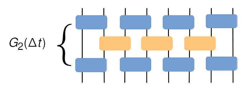
Each two site MPO in Fig 14 is of the form and can be approximated as . obtained numerically can be expanded as where and .