跳到论文正文
W Papers独立论文阅读器 arXiv:2012.09754 论文正文 计算阅读时间 · 0%
引用这篇论文根据当前论文元数据生成,正式投稿前建议核对。


License: arXiv.org perpetual non-exclusive license
arXiv:2012.09754v1 [math.CA] 17 Dec 2020

Harmonic intrinsic graphs in the Heisenberg groupThanks:  This material is based upon work supported by the National Science Foundation under Grant Nos. 2005609 and 1926686 and research done while the author was a visiting member at the Institute of Advanced Study.

Robert Young Address: New York University, Courant Institute of Mathematical Sciences, 251 Mercer Street, New York, NY 10012, USA. Email address: ryoung@cims.nyu.edu
Abstract.

Minimal surfaces in ℝn\mathbb{R}^{n} can be locally approximated by graphs of harmonic functions, i.e., functions that are critical points of the Dirichlet energy, but no analogous theorem is known for HH–minimal surfaces in the three-dimensional Heisenberg group ℍ\mathbb{H}, which are known to have singularities. In this paper, we introduce a definition of intrinsic Dirichlet energy for surfaces in ℍ\mathbb{H} and study the critical points of this energy, which we call contact harmonic graphs. Nearly flat regions of HH–minimal surfaces can often be approximated by such graphs. We give a calibration condition for an intrinsic Lipschitz graph to be energy-minimizing, construct energy-minimizing graphs with a variety of singularities, and prove a first variation formula for the energy of intrinsic Lipschitz graphs and piecewise smooth intrinsic graphs.

1. Introduction

Minimal surfaces in ℝ3\mathbb{R}^{3} are smooth, but the analogous HH–minimal surfaces in the three-dimensional Heisenberg group need not be. Recall that an HH–minimal surface is a stationary point of the Heisenberg area functional, which is proportional to the 33–dimensional spherical Hausdorff measure. There are many examples of HH–minimal surfaces with a singularity along a curve [Pau06], as shown in Figure 1.
Refer to caption
Refer to caption
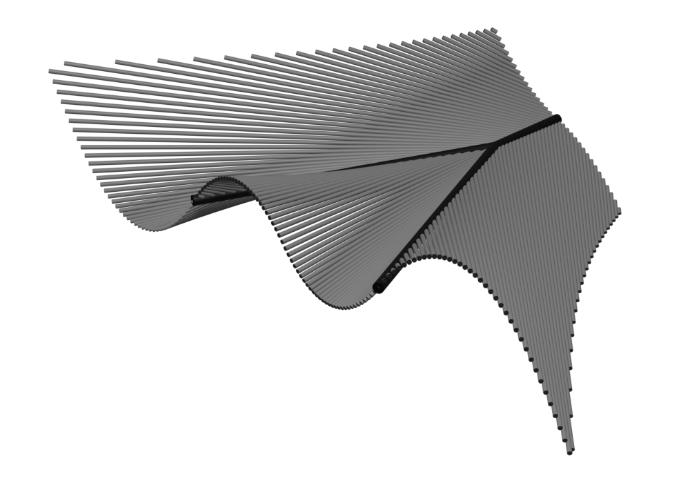
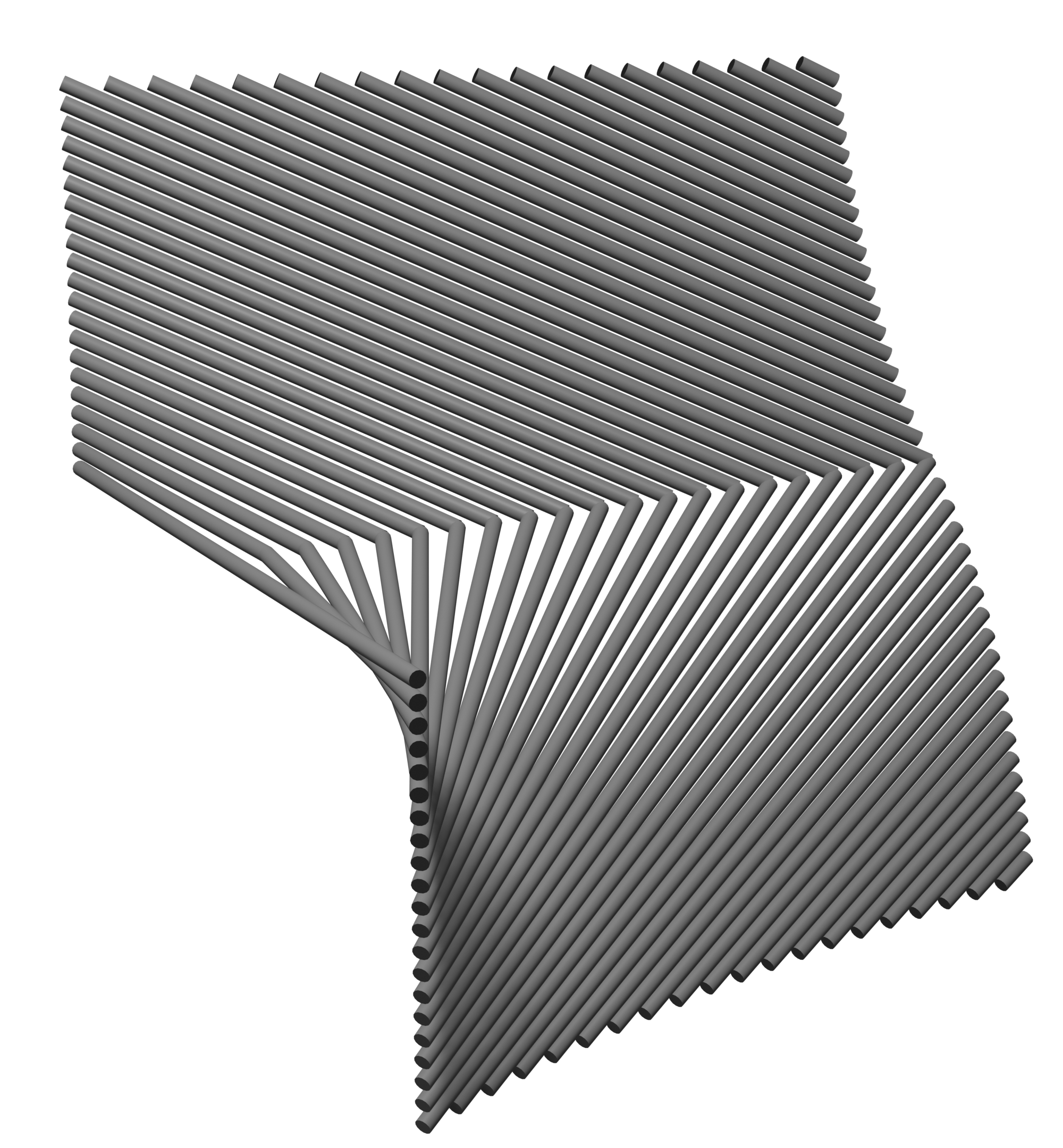
Figure 1. Examples of HH–minimal and contact harmonic graphs with singularities. In both cases, the surfaces consist of horizontal line segments which intersect only along the characteristic nexus. 33D models can be found in the supplementary materials.
Refer to caption
Figure 2. An HH–minimal graph with branched characteristic nexus (left) and the foliation of Σ\Sigma by horizontal curves, projected to the x​yxy–plane (right). Dashed lines mark the boundaries between the pieces of herringbone surfaces (see Lemma 3.5) that make up Σ\Sigma and thick lines mark the characteristic nexus. A 33D model of the surface can be found in the supplementary materials.

In fact, HH–minimal surfaces can have singularities in regions that are close to flat. The surfaces in Figure 1, for example, grow closer to planes as one moves from left to right. Subtler examples come from a construction of Nicolussi Golo and Ritoré [NGR20].

Theorem 1.1 ([NGR20]).

Let S1S^{1} be the unit circle of horizontal vectors in ℍ\mathbb{H}. Given a collection (finite or countably infinite) of disjoint nonempty open intervals I1,I2,⋯⊂S1I_{1},I_{2},\dots\subset S^{1} such that ℓ⁡(Ii)<2​π\ell(I_{i})<2\pi for all ii, let K=S1∖⋃iIiK=S^{1}\smallsetminus\bigcup_{i}I_{i} be its complement. Let Ii=(ai,bi)I_{i}=(a_{i},b_{i}) and let mi∈S1m_{i}\in S^{1} be the midpoint of IiI_{i}. Let ΣK\Sigma_{K} be the surface consisting of the union of:

  • •

    for each k∈Kk\in K, a horizontal ray from the origin in the direction of kk,

  • •

    for each ii, a horizontal ray RiR_{i} from the origin in the direction of mim_{i}, and

  • •

    for each p∈Rip\in R_{i}, a pair of horizontal rays from pp in the directions of aia_{i} and bib_{i}.

Then ΣK\Sigma_{K} is a scale-invariant area-minimizing surface.

Figure 2 shows an example of such a surface; here, the rays RiR_{i} are the thick lines and KK consists of the three points in S1S^{1} corresponding to the dashed lines.

If we bring these three points close together, ΣK\Sigma_{K} converges to a vertical plane; one can show (see Proposition 1.3) that if K={−ε,0,ε}K=\{-\varepsilon,0,\varepsilon\}, then ΣK\Sigma_{K} converges to the x​zxz–plane as ε→0\varepsilon\to 0. That is, ΣK\Sigma_{K} can be arbitrarily close to the x​zxz–plane in ℍ\mathbb{H} and still have a branched singularity.

In fact, there are examples with worse behavior. Suppose that KK is a Cantor set with positive measure and let χ=⋃Ri\chi=\bigcup R_{i}. Since KK is a Cantor set, the closure χ¯\overline{\chi} contains the cone over KK, which has positive measure. The rectifiability of ΣK\Sigma_{K} implies that almost every point in χ¯\overline{\chi} has a vertical approximate tangent plane; indeed, this holds for every point in χ¯∖χ\overline{\chi}\smallsetminus\chi. If p∈χ¯∖χp\in\overline{\chi}\smallsetminus\chi, then ΣK\Sigma_{K} is flat near pp in the sense that the neighborhoods ΣK∩B⁡(p,ε)\Sigma_{K}\cap B(p,\varepsilon) are close to a vertical plane for sufficiently small ε\varepsilon, but singular in the sense that ΣK∩B⁡(p,ε)\Sigma_{K}\cap B(p,\varepsilon) is nonsmooth for all ε\varepsilon and the unit horizontal normal to ΣK∩B⁡(p,ε)\Sigma_{K}\cap B(p,\varepsilon) is discontinuous.

This does not happen in ℝn\mathbb{R}^{n}. A key step in proving the regularity of codimension–11 minimal surfaces in ℝn\mathbb{R}^{n} is to show that if EE is a perimeter-minimizing subset of ℝn\mathbb{R}^{n} and pp lies in the reduced boundary of EE, then ∂E\partial E can be approximated by graphs of harmonic functions on small balls around pp. One can then use the regularity of harmonic functions to show that ∂E\partial E is smooth on sufficiently small balls around pp; see for instance [Mag12] for an exposition.

In this paper, we propose a method to study singular points in HH–minimal surfaces by using an analogue of harmonic functions that we call contact harmonic graphs. Many of these graphs arise as limits of HH–minimal surfaces under rescaling and stretching, and we conjecture that, as in ℝn\mathbb{R}^{n}, one can use harmonic graphs to approximate sufficiently flat regions of HH–minimal surfaces. A harmonic graph is a critical point of the intrinsic Dirichlet energy (see (1)); we describe a calibration method to prove that a graph is energy-minimizing and use calibrations to construct several examples. In addition, we prove a first variation formula for the intrinsic Dirichlet energy that lets us characterize intrinsic Lipschitz harmonic graphs.

Before we state our results, we set some notation. We define the Heisenberg group ℍ\mathbb{H} to be the set ℝ3\mathbb{R}^{3} equipped with the product

(x,y,z)⋅(x′,y′,z′)=(x+x′,y+y′,z+z′+x​y′−y​x′2).(x,y,z)\cdot(x^{\prime},y^{\prime},z^{\prime})=\left(x+x^{\prime},y+y^{\prime},z+z^{\prime}+\frac{xy^{\prime}-yx^{\prime}}{2}\right).

Let x,y,z:ℍ→ℝx,y,z\colon\mathbb{H}\to\mathbb{R} be the coordinate functions and let X,Y,ZX,Y,Z be the coordinate vectors. The one-parameter subgroups of ℍ\mathbb{H} generated by these vectors are the coordinate axes, so we write elements of these one-parameter subgroups as Xt=(t,0,0)X^{t}=(t,0,0), Yt=(0,t,0)Y^{t}=(0,t,0), and Zt=(0,0,t)Z^{t}=(0,0,t), for t∈ℝt\in\mathbb{R}. Let V0={(x,y,z)∈ℍ:y=0}V_{0}=\{(x,y,z)\in\mathbb{H}:y=0\} be the x​zxz–plane. For any f:V0→ℝf\colon V_{0}\to\mathbb{R}, we define the intrinsic graph of ff to be

Γf={v⋅Yf⁡(v):v∈V0}\Gamma_{f}=\{v\cdot Y^{f(v)}:v\in V_{0}\}

and define Ψf:V0→Γf\Psi_{f}\colon V_{0}\to\Gamma_{f} by Ψf​(v)=v⋅Yf⁡(v)\Psi_{f}(v)=v\cdot Y^{f(v)}. Let μ\mu be Lebesgue measure on V0V_{0}.

When ff is an intrinsic Lipschitz function (see Definition 2.1), Γf\Gamma_{f} has approximate tangent planes with respect to the Carnot–Carathéodory metric almost everywhere [FSSC11] and these planes are vertical (parallel to the zz–axis). Each tangent plane projects to a line in the x​yxy–plane with slope given by a nonlinear differential operator, the intrinsic gradient. When ff is smooth, the intrinsic gradient of ff is given by

∇ff=(∂x−f∂z)f;\nabla_{f}f=(\partial_{x}-f\partial_{z})f;

when ff is not smooth, we define ∇ff\nabla_{f}f in the distributional sense (see Definition 2.2).

Given a bounded open subset U⊂V0U\subset V_{0} and an intrinsic graph Γ⊂ℍ\Gamma\subset\mathbb{H}, we define the intrinsic Dirichlet energy of Γ\Gamma on UU by

EU​(Γ)=12​∫U|∇ff|2​𝑑μ,E_{U}(\Gamma)=\frac{1}{2}\int_{U}|\nabla_{f}f|^{2}\,\mathrm{d}\mu, (1)

where μ\mu is Lebesgue measure on V0V_{0}.

By [CMPSC14, Thm. 1.6], the spherical Hausdorff measure11 1 Unless otherwise specified, distances and Hausdorff measures in ℍ\mathbb{H} will be with respect to the Carnot–Carathèodory metric. of an intrinsic Lipschitz graph Γ=Γf\Gamma=\Gamma_{f} of f:U→ℝf\colon U\to\mathbb{R} can be written

𝒮3​(Γ)=∫U1+|∇ff|2​𝑑μ.\mathcal{S}^{3}(\Gamma)=\int_{U}\sqrt{1+|\nabla_{f}f|^{2}}\,\mathrm{d}\mu. (2)

In fact, the formula includes a multiplicative constant, but throughout this paper, we will normalize 𝒮3\mathcal{S}^{3} so that (2) holds without a constant. When ∇ff\nabla_{f}f is small,

𝒮3​(Γ)=∫U1+12​|∇ff|2+O⁡(|∇ff|3)​𝑑μ=μ⁡(U)+EU​(Γ)+O⁡(μ⁡(U)​‖∇ff‖∞3),\mathcal{S}^{3}(\Gamma)=\int_{U}1+\frac{1}{2}|\nabla_{f}f|^{2}+O(|\nabla_{f}f|^{3})\,\mathrm{d}\mu=\mu(U)+E_{U}(\Gamma)+O(\mu(U)\|\nabla_{f}f\|_{\infty}^{3}), (3)

so when ∇ff\nabla_{f}f is small, the intrinsic Dirichlet energy of Γ\Gamma is closely linked to its area.

This suggests that an area-minimizing surface with small ∇ff\nabla_{f}f should be close to energy-minimizing. We can formalize this notion using stretch automorphisms. For r>0r>0, the map s=sr−1,r​(x,y,z)=(r−1​x,r​y,z)s=s_{r^{-1},r}(x,y,z)=(r^{-1}x,ry,z) is an automorphism of ℍ\mathbb{H} that sends intrinsic graphs to intrinsic graphs and multiplies ∇ff\nabla_{f}f by r2r^{2}. Since its Jacobian on V0V_{0} is r−1r^{-1}, Es⁡(U)​(s⁡(Γ))=r3​EU​(Γ)E_{s(U)}(s(\Gamma))=r^{3}E_{U}(\Gamma). One can use this to construct energy-minimizing surfaces; if Γ1,Γ2,…\Gamma_{1},\Gamma_{2},\dots, are area-minimizing surfaces and Λ\Lambda is such that si−1,i​(Γi)=Λs_{i^{-1},i}(\Gamma_{i})=\Lambda for all ii, then Λ\Lambda is energy-minimizing. This shows, for instance, that if f⁡(x,z)=−a​z​sign⁡(z)f(x,z)=-a\sqrt{z}\sign(z) for some a≠0a\neq 0, then Γf\Gamma_{f} is energy-minimizing (Lemma 3.5). These surfaces were studied in [Pau06, CHY07, MSCV08]; we call them herringbone surfaces, since they can be written as the union of horizontal rays that branch out from the xx–axis in a herringbone pattern.

The area-minimizing cones constructed in [NGR20] also have energy-minimizing analogues. As in [NGR20], these surfaces can be written as a union of horizontal rays that either end at the origin or branch off of the singular set; the renderings in the figures are made up of these rays. The slope of a horizontal ray is defined as the slope of its projection to the x​yxy–plane; a horizontal ray is positive or negative depending on whether it points in the +x+x– or −x-x–direction.

Theorem 1.2.

Let α>0\alpha>0. Let I1,I2,⋯⊂[−α,α]I_{1},I_{2},\dots\subset[-\alpha,\alpha] be a collection of disjoint nonempty open intervals, and let K=[−α,α]∖⋃IiK=[-\alpha,\alpha]\smallsetminus\bigcup I_{i}. Let Ii=(ai,bi)I_{i}=(a_{i},b_{i}) and let mi=ai+bi2m_{i}=\frac{a_{i}+b_{i}}{2}. Let ΛK⊂ℍ\Lambda_{K}\subset\mathbb{H} be the surface consisting of the union of:

  1. (1)

    the negative xx–axis, denoted R0R_{0},

  2. (2)

    for each k∈Kk\in K, a positive horizontal ray from the origin with slope kk,

  3. (3)

    for each i⩾1i\geqslant 1, a positive horizontal ray RiR_{i} from the origin with slope mim_{i}, and

  4. (4)

    for each p∈R0p\in R_{0}, a pair of positive horizontal rays from pp with slopes α\alpha and −α-\alpha.

  5. (5)

    for each p∈Ri,i⩾1p\in R_{i},i\geqslant 1, a pair of positive horizontal rays from pp with slopes aia_{i} and bib_{i}.

Then ΛK\Lambda_{K} is a scale-invariant energy-minimizing surface.

Since α=supK\alpha=\sup K and −α=infK-\alpha=\inf K, ΛK\Lambda_{K} is uniquely determined by KK.

Refer to caption
Figure 3. An energy-minimizing graph based on the middle-thirds Cantor set KK. The top figure shows the foliation of ΛK\Lambda_{K} by horizontal curves, projected to the x​yxy–plane. In the shaded regions, the surface coincides with the horizontal plane through 𝟎\mathbf{0}. The bottom figure shows the cross-section of the surface in the vertical plane marked by the dashed line; the surface coincides with the x​yxy–plane in the flat regions. A 33D model of the surface can be found in the supplementary materials.

Any such ΛK\Lambda_{K} can be written as a limit of stretched area-minimizing surfaces.

Proposition 1.3.

Let α\alpha, K=[−α,α]∖⋃IiK=[-\alpha,\alpha]\smallsetminus\bigcup I_{i} be as in Theorem 1.2. We identify S1S^{1} with the interval (−π,π](-\pi,\pi] so that the +x+x–axis is identified with 00. For n>αn>\sqrt{\alpha}, let Kn=n−2​KK_{n}=n^{-2}K and let Sn=ΣKnS_{n}=\Sigma_{K_{n}} be the corresponding area-minimizing surface constructed in Theorem 1.1.

Let Sn+S_{n}^{+} and ΛK+\Lambda_{K}^{+} be the half-spaces bounded by SnS_{n} and ΛK\Lambda_{K}. Then 𝟏Sn+→𝟏ΛK+\mathbf{1}_{S_{n}^{+}}\to\mathbf{1}_{\Lambda_{K}^{+}} in L1loc​(ℍ)L_{1}^{\mathrm{loc}}(\mathbb{H}).

Conversely, one may ask when a sequence of stretched area-minimizing surfaces has a subsequence that converges to an energy-minimizing surface. We first define the horizontal excess of a set; the horizontal excess of the half-space bounded by a graph is related to the energy of that graph, but the horizontal excess is defined for a larger class of sets. Let E⊂ℍE\subset\mathbb{H} be a subset with finite perimeter and horizontal normal νE\nu_{E}. For p∈∂Ep\in\partial E, r>0r>0, and a horizontal vector ν∈S1\nu\in S^{1}, we define

ExcB⁡(p,r)⁡(E,ν)\displaystyle\Exc_{B(p,r)}(E,\nu) =1r3​∫B⁡(p,r)|νE​(p)−ν|2​d​|∂E|​(p)\displaystyle=\frac{1}{r^{3}}\int_{B(p,r)}|\nu_{E}(p)-\nu|^{2}\,\mathrm{d}|\partial E|(p)
ExcB⁡(p,r)⁡(E)\displaystyle\Exc_{B(p,r)}(E) =infν∈S1ExcB⁡(p,r)⁡(E,ν),\displaystyle=\inf_{\nu\in S^{1}}\Exc_{B(p,r)}(E,\nu),

where |∂E||\partial E| is the perimeter measure of EE (Section 2.4). Monti [Mon14] showed that if EE is perimeter-minimizing and if ExcB⁡(p,r)⁡(E)\Exc_{B(p,r)}(E) is sufficiently small for some p∈∂Ep\in\partial E, r>0r>0, then ∂E\partial E can be approximated by an intrinsic Lipschitz graph near pp, and the energy of this graph

Question 1.4.

Let c,k>0c,k>0. Suppose that ri→∞r_{i}\to\infty and E1,E2,⋯⊂ℍE_{1},E_{2},\dots\subset\mathbb{H} are a sequence of sets that are perimeter-minimizing in the stretched balls Wi=sri,ri−1​(B⁡(𝟎,k))W_{i}=s_{r_{i},r_{i}^{-1}}(B(\mathbf{0},k)). Let E^i=sri,ri−1−1​(Ei)\hat{E}_{i}=s_{r_{i},r_{i}^{-1}}^{-1}(E_{i}) and suppose that ExcB⁡(𝟎,k)⁡(E^i,Y)<c\Exc_{B(\mathbf{0},k)}(\hat{E}_{i},Y)<c for all ii. Is it possible to choose cc and kk such that a subsequence of the E^i\hat{E}_{i}’s converge to a set EE such that ∂E\partial E is energy-minimizing or contact harmonic on B⁡(𝟎,1)B(\mathbf{0},1)?

(For the definition of contact harmonic, see below.)

One might approach this question by noting that the excess ExcB⁡(Ei,Y)<c\Exc_{B}(E_{i},Y)<c must be small for appropriate balls in WiW_{i}, so the results of [Mon14] give an intrinsic Lipschitz half-space Γi+\Gamma_{i}^{+} that approximates EiE_{i}. Then Γ^i+=sri,ri−1−1​(Γi+)\hat{\Gamma}^{+}_{i}=s_{r_{i},r_{i}^{-1}}^{-1}(\Gamma^{+}_{i}) is a graph approximating E^i\hat{E}_{i}’s, and one can hope for the corresponding functions to converge.

The problem, however, is that though the intrinsic Lipschitz constants of the Γi\Gamma_{i}’s are uniformly bounded, the intrinsic Lipschitz constants of the Γ^i\hat{\Gamma}_{i}’s are not. At best, if hih_{i} is the function such that Γ^i=Γhi\hat{\Gamma}_{i}=\Gamma_{h_{i}}, then hih_{i} satisfies an intrinsic Sobolev bound like

∫D(∇hihi)2​𝑑μ⩽C\int_{D}(\nabla_{h_{i}}h_{i})^{2}\,\mathrm{d}\mu\leqslant C

on an appropriate domain D⊂V0D\subset V_{0}. Not much is known about such functions, and more research may be necessary to answer Question 1.4.

Another approach to Question 1.4 is to study other characterizations of energy-minimizing graphs. In an analogue to the usual notion of harmonicity, we define a contact harmonic graph to be a critical point of the energy with respect to a class of deformations called contact deformations. In particular, energy-minimizing graphs are contact harmonic. In Section 4, we prove some tools for working with such graphs, including first variation formulas for the energy of smooth and intrinsic Lipschitz graphs. These formulas lead to the following characterization of contact harmonicity.

Theorem 1.5.

A smooth intrinsic graph Γ=Γf\Gamma=\Gamma_{f} is contact harmonic on U⊂V0U\subset V_{0} (a critical point of the energy with respect to contact variations supported on UU) if and only if

2​∂zf⋅∇f2f−∇f3f=02\partial_{z}f\cdot\nabla_{f}^{2}f-\nabla_{f}^{3}f=0 (4)

on UU.

For an intrinsic Lipschitz function ff and for w∈Cc∞​(U)w\in C^{\infty}_{c}(U), let

Δf​w=∇f[∂xw]−∇ff⋅∂zw−f​∇f[∂zw].\Delta_{f}w=\nabla_{f}[\partial_{x}w]-\nabla_{f}f\cdot\partial_{z}w-f\nabla_{f}[\partial_{z}w].

(When ff is smooth, Δf​w=∇f2w\Delta_{f}w=\nabla_{f}^{2}w.) Let

B2​(f,w)\displaystyle B_{2}(f,w) =−Δfw⋅∇ff+12(∇ff)2⋅∂zw,\displaystyle=-\Delta_{f}w\cdot\nabla_{f}f+\frac{1}{2}(\nabla_{f}f)^{2}\cdot\partial_{z}w,
B1​(f,w)\displaystyle B_{1}(f,w) =f​B2​(f,w)−32​(∇ff)2⋅∇fw,\displaystyle=fB_{2}(f,w)-\frac{3}{2}(\nabla_{f}f)^{2}\cdot\nabla_{f}w,

Then Γ=Γf\Gamma=\Gamma_{f} is contact harmonic on UU if and only if

∫UB1​(f,w)​𝑑μ=∫UB2​(f,w)​𝑑μ=0\int_{U}B_{1}(f,w)\,\mathrm{d}\mu=\int_{U}B_{2}(f,w)\,\mathrm{d}\mu=0

for every w∈Cc∞​(U)w\in C^{\infty}_{c}(U).

This theorem follows from Theorem 4.5 (in the smooth case) and Theorem 4.8 (in the intrinsic Lipschitz case).

Condition (4) is weaker than the condition that the horizontal mean curvature of Γf\Gamma_{f} vanishes (i.e., ∇f2​f=0\nabla_{f}^{2}f=0). Indeed, Theorem 1.5 implies that the surface Γf={(x,y,z)∈ℍ:y=x2}\Gamma_{f}=\{(x,y,z)\in\mathbb{H}:y=x^{2}\}, which has ∇f2​f=2\nabla_{f}^{2}f=2, is contact harmonic. This happens because contact harmonic graphs are energy-stationary only for contact diffeomorphisms, not arbitrary diffeomorphisms. Contact diffeomorphisms preserve horizontality, so they also preserve horizontal connectivity. That is, if ϕ:ℍ→ℍ\phi\colon\mathbb{H}\to\mathbb{H} is a contact diffeomorphism and if p,q∈Γp,q\in\Gamma are connected by a horizontal curve in Γ\Gamma, then ϕ⁡(p)\phi(p) and ϕ⁡(q)\phi(q) are connected by a horizontal curve in ϕ⁡(Γ)\phi(\Gamma). A contact harmonic graph may admit smooth deformations that reduce its energy, but these smooth deformations affect the horizontal connectivity of the graph. 22 2 Manuel Ritoré informs us that the cylinder {x2+y2=r2}\{x^{2}+y^{2}=r^{2}\} is an area-stationary analogue of this example, i.e. a smooth surface in ℍ\mathbb{H} with nonzero horizontal mean curvature that is area-stationary under contact deformations, but as far as we are aware, the calculation has not been published.

We use the first-variation formula for smooth graphs to prove a first variation formula for piecewise smooth graphs (Theorem 4.11). This shows that if Γ\Gamma is a piecewise smooth contact harmonic graph whose characteristic nexus is a curve and if the foliation by horizontal curves is well-behaved near the characteristic nexus, then the slope of the characteristic nexus is the average of the slopes of the horizontal curves on either side of the nexus. Such singularities are similar to the singularities of HH–minimal surfaces studied in [Pau06, CHY07].

Finally, we conclude with an observation. One motivation for this work was the Bernstein problem for surfaces with low regularity. Bernstein’s Theorem states that an area-minimizing codimension–11 graph in ℝn\mathbb{R}^{n} is a plane. The Bernstein problem asks for conditions under which other classes of area-minimizing surfaces are planes. Barone Adesi, Serra Cassano, and Vittone showed that if Γ⊂ℍ\Gamma\subset\mathbb{H} is a area-minimizing intrinsic graph of an entire C2C^{2} function, then Γ\Gamma is a vertical plane [BASCV07]. The same result for C1C^{1} functions was proved by Galli and Ritoré [GR15], and for locally Lipschitz functions by Nicolussi Golo and Serra Cassano [NSC19], but there are many examples of area-minimizing intrinsic Lipschitz graphs that are not vertical planes, such as many of the examples in Section 3. All of these examples, however, are also entire ZZ–graphs, i.e., sets of the form {(x,y,g(x,y))∈ℍ:x,y∈ℝ}\{(x,y,g(x,y))\in\mathbb{H}:x,y\in\mathbb{R}\}. One may then ask the following:

Question 1.6.

Is every nonplanar entire area-minimizing (or energy-minimizing) intrinsic Lipschitz graph also a ZZ–graph?

Remark 1.7.

The 3D models used in the figures in this paper can be found in .obj format in the ancillary files on the arXiv page for this paper. These files can be opened in Preview on Macs, Paint 3D on Windows, or any 3D modeling program. They can also be found at https://cims.nyu.edu/˜ryoung/harmonic/.

1.1. Outline of paper

In Section 2, we establish notation for the Heisenberg group and prove some integration formulas which will be used throughout the paper. In Section 3, we define the intrinsic Dirichlet energy, prove some basic properties of energy-minimizing surfaces, and describe a method to prove that a surface is energy-minimizing using a calibration. We use this method to prove Theorem 1.2 and Proposition 1.3. In Section 4, we define contact variations and contact harmonicity and prove first variation formulas for the energy of smooth graphs and intrinsic Lipschitz graphs, including Theorem 1.5. Many energy-minimizing and area-minimizing surfaces have singularities along curves, which we call herringbone singularities, and we prove a first variation formula for the energy of such a graph in Section 4.2.

The author would like to thank Roberto Monti, Sebastiano Nicolussi Golo, Manuel Ritoré, and Davide Vittone for their helpful discussions during the preparation of this paper and to thank the Institute of Advanced Study for its hospitality.

2. Preliminaries

Throughout this paper, we use the following standard conventions for asymptotic notation. The notations f≲gf\lesssim g and g≳fg\gtrsim f mean that f⩽C​gf\leqslant Cg for some universal constant C∈(0,∞)C\in(0,\infty), and f≍gf\asymp g means that f≲gf\lesssim g and g≲fg\lesssim f. If CC depends on some parameters, we indicate this by subscripts, i.e., f≲tgf\lesssim_{t}g implies that f⩽C​gf\leqslant Cg where C=C⁡(t)C=C(t) depends only on tt. Finally, we use big–OO notation O⁡(f)O(f) to denote an error term whose absolute value is bounded by a universal constant multiple of |f||f|.

2.1. The Heisenberg group

The Heisenberg group ℍ\mathbb{H} is the 33–dimensional simply connected Lie group with Lie algebra

𝔥:=⟨X,Y,Z:[X,Y]=Z,[X,Z]=[Y,Z]=0⟩.\mathfrak{h}:=\langle X,Y,Z:[X,Y]=Z,[X,Z]=[Y,Z]=0\rangle.

We identify ℍ\mathbb{H} with its Lie algebra via the Baker–Campbell–Hausdorff formula, i.e., ℍ=⟨X,Y,Z⟩≅ℝ3\mathbb{H}=\langle X,Y,Z\rangle\cong\mathbb{R}^{3} and

(x,y,z)⋅(x′,y′,z′)=(x+x′,y+y′,z+z′+x​y′−y​x′2).(x,y,z)\cdot(x^{\prime},y^{\prime},z^{\prime})=\left(x+x^{\prime},y+y^{\prime},z+z^{\prime}+\frac{xy^{\prime}-yx^{\prime}}{2}\right).

We use XX, YY, and ZZ to denote the coordinate vectors of ℝ3\mathbb{R}^{3} and the corresponding left-invariant fields X(x,y,z)=(1,0,−y2)X_{(x,y,z)}=(1,0,-\frac{y}{2}), Y(x,y,z)=(0,1,x2)Y_{(x,y,z)}=(0,1,\frac{x}{2}), and Z(x,y,z)=(0,0,1)Z_{(x,y,z)}=(0,0,1). We write the coordinate vector fields in ℝ3\mathbb{R}^{3} as ∂x\partial_{x}, ∂y\partial_{y}, and ∂z=Z\partial_{z}=Z. Every vector v∈ℍv\in\mathbb{H} generates a one-parameter subgroup of ℍ\mathbb{H}; we write ⟨v⟩=ℝ​v\langle v\rangle=\mathbb{R}v for this subgroup and define vt=t​vv^{t}=tv for all t∈ℝt\in\mathbb{R}.

Let 𝖠=span⁡(X,Y)\mathsf{A}=\spanop(X,Y) be the left-invariant distribution spanned by XX and YY; we refer to this as the horizontal distribution. Curves that are Lipschitz (with respect to the Euclidean metric) and almost everywhere tangent to 𝖠\mathsf{A} are called horizontal curves. For h∈ℍh\in\mathbb{H} and (a,b)∈ℝ2∖(0,0)(a,b)\in\mathbb{R}^{2}\smallsetminus(0,0), we call the line L=h⋅⟨a​X+b​Y⟩L=h\cdot\langle aX+bY\rangle a horizontal line. Let π:ℍ→ℝ2\pi\colon\mathbb{H}\to\mathbb{R}^{2} be the projection π⁡(x,y,z)=(x,y)\pi(x,y,z)=(x,y); we will identify ℝ2\mathbb{R}^{2} with the x​yxy–plane in ℍ\mathbb{H}. The slope of a horizontal line LL is the slope of the projection π⁡(L)\pi(L), i.e., ba\frac{b}{a}, as long as a≠0a\neq 0. A vertical plane V⊂ℍV\subset\mathbb{H} is a plane parallel to ⟨Z⟩\langle Z\rangle; its slope is the slope of the projection π⁡(V)\pi(V).

Let dd represent the Carnot–Carathéodory metric on ℍ\mathbb{H}. That is, we define a norm on 𝖠\mathsf{A} by ‖a​X+b​Y‖=a2+b2\|aX+bY\|=\sqrt{a^{2}+b^{2}}, and given a horizontal curve γ:I→ℍ\gamma\colon I\to\mathbb{H}, we define the length of γ\gamma as

ℓ⁡(γ)=ℓℝ2​(π∘γ)=∫I‖γ′​(t)‖​𝑑t.\ell(\gamma)=\ell_{\mathbb{R}^{2}}(\pi\circ\gamma)=\int_{I}\|\gamma^{\prime}(t)\|\,\mathrm{d}t.

For p,q∈ℍp,q\in\mathbb{H}, let d⁡(p,q)=infγℓ⁡(γ)d(p,q)=\inf_{\gamma}\ell(\gamma), where the infimum is taken over all horizontal curves γ:[0,1]→ℍ\gamma\colon[0,1]\to\mathbb{H} such that γ⁡(0)=p\gamma(0)=p and γ⁡(1)=q\gamma(1)=q. This is a left-invariant metric that satisfies the ball-box inequality

d⁡(𝟎,p)≍max⁡{|x⁡(p)|,|y⁡(p)|,|z⁡(p)|}.d(\mathbf{0},p)\asymp\max\{|x(p)|,|y(p)|,\sqrt{|z(p)|}\}. (5)

This metric gives ℍ\mathbb{H} Hausdorff dimension 44, and a smooth codimension–11 surface or intrinsic Lipschitz graph (Definition 2.1) has Hausdorff dimension 33. Let 𝒮d\mathcal{S}^{d} be the spherical Hausdorff dd–measure, normalized so that 𝒮4\mathcal{S}^{4} is Lebesgue measure on ℍ\mathbb{H} and the restriction of 𝒮3\mathcal{S}^{3} to the x​zxz–plane is Lebesgue measure on the x​zxz–plane.

2.2. Intrinsic graphs

Let V0={(x,y,z)∈ℍ:y=0}V_{0}=\{(x,y,z)\in\mathbb{H}:y=0\} be the x​zxz–plane. For any U⊂V0U\subset V_{0} and any f:U→ℝf\colon U\to\mathbb{R}, the intrinsic graph of ff is the set

Γf={v⋅Yf⁡(v):v∈U}.\Gamma_{f}=\{v\cdot Y^{f(v)}:v\in U\}.

Let Ψf:U→Γf\Psi_{f}\colon U\to\Gamma_{f} be the map Ψf​(v)=v⋅Yf⁡(v)\Psi_{f}(v)=v\cdot Y^{f(v)}. Let Π:ℍ→V0\Pi\colon\mathbb{H}\to V_{0},

Π⁡(x,y,z)=(x,y,z)⋅Y−y=(x,0,z−x​y2).\Pi(x,y,z)=(x,y,z)\cdot Y^{-y}=\left(x,0,z-\frac{xy}{2}\right). (6)

This is the projection to V0V_{0} whose fibers are the cosets of ⟨Y⟩\langle Y\rangle. The restrictions Π|Γf\Pi|_{\Gamma_{f}} and Ψf|U\Psi_{f}|_{U} are bijections (homeomorphisms when ff is continuous), and Π∘Ψf=idU\Pi\circ\Psi_{f}=\id_{U}.

Let γ=(γx,γy,γz):I→ℍ\gamma=(\gamma_{x},\gamma_{y},\gamma_{z})\colon I\to\mathbb{H} be a horizontal curve such that γ\gamma has unit xx–speed, i.e., γx′=1\gamma_{x}^{\prime}=1. For almost every t∈It\in I,

γ′​(t)=γx′​(t)​Xγ⁡(t)+γy′​(t)​Yγ⁡(t)=Xγ⁡(t)+γy′​(t)​Yγ⁡(t).\gamma^{\prime}(t)=\gamma^{\prime}_{x}(t)X_{\gamma(t)}+\gamma^{\prime}_{y}(t)Y_{\gamma(t)}=X_{\gamma(t)}+\gamma^{\prime}_{y}(t)Y_{\gamma(t)}.

For any p∈ℍp\in\mathbb{H}, we have Π∗(Xp)=∂x−y(p)∂z\Pi_{*}(X_{p})=\partial_{x}-y(p)\partial_{z} and Π∗​(Yp)=0\Pi_{*}(Y_{p})=0, so

(Π∘γ)′(t)=Π∗(Xγ⁡(t))+γy′(t)Π∗(Yγ⁡(t))=∂x−γy(t)∂z.(\Pi\circ\gamma)^{\prime}(t)=\Pi_{*}(X_{\gamma(t)})+\gamma^{\prime}_{y}(t)\Pi_{*}(Y_{\gamma(t)})=\partial_{x}-\gamma_{y}(t)\partial_{z}. (7)

That is, one can reconstruct γ\gamma from the projection Π∘γ\Pi\circ\gamma.

Franchi, Serapioni, and Serra Cassano [FSSC06] defined the class of intrinsic Lipschitz graphs, which are analogues of graphs of Lipschitz functions in ℝn\mathbb{R}^{n}. We will give a definition which is equivalent to theirs, but with a different value for the Lipschitz constant [Rig19].

Definition 2.1.

Let Γ=Γf⊂ℍ\Gamma=\Gamma_{f}\subset\mathbb{H} be an intrinsic graph and let λ∈(0,1)\lambda\in(0,1). We say that Γ\Gamma is an intrinsic λ\lambda–Lipschitz graph (and that ff is an intrinsic λ\lambda–Lipschitz function) if for every p,q∈Γp,q\in\Gamma,

|y⁡(q)−y⁡(p)|⩽λ​d​(p,q).|y(q)-y(p)|\leqslant\lambda d(p,q).

If Π⁡(Γf)=V0\Pi(\Gamma_{f})=V_{0}, or equivalently, if the domain of ff is all of V0V_{0}, we say that Γf\Gamma_{f} is an entire intrinsic Lipschitz graph. Every intrinsic Lipschitz graph is a subset of an entire intrinsic Lipschitz graph; see [NY18, Thm. 27] and [Rig19].

Let Γ=Γf\Gamma=\Gamma_{f} be an intrinsic Lipschitz graph. Let ∇f\nabla_{f} be the vector field on V0V_{0} given by ∇f=∂x−f∂z\nabla_{f}=\partial_{x}-f\partial_{z}. We call the corresponding operator the intrinsic gradient. For every point p∈Γp\in\Gamma, there is a (possibly non-unique) unit xx–speed horizontal curve γ=(γx,γy,γz):ℝ→Γ\gamma=(\gamma_{x},\gamma_{y},\gamma_{z})\colon\mathbb{R}\to\Gamma such that γ⁡(0)=p\gamma(0)=p. We call the projection λ=Π∘γ\lambda=\Pi\circ\gamma of such a curve to V0V_{0} a characteristic curve of Γ\Gamma. By (7), every characteristic curve is an integral curve of γ\gamma; conversely, by Theorems 1.1 and 1.2 of [BCSC15], every integral curve of γ\gamma is the projection of a unit xx–speed horizontal curve. Thus the characteristic curves are exactly the integral curves of ∇f\nabla_{f}. When ff is smooth, there is a unique characteristic curve passing through every point of V0V_{0}, and the intrinsic gradient is the derivative along these characteristic curves.

The intrinsic gradient ∇ff\nabla_{f}f of ff is particularly important. When ff is smooth and v∈V0v\in V_{0}, ∇ff​(v)\nabla_{f}f(v) is the slope of the unique horizontal curve through p=Ψf​(v)p=\Psi_{f}(v). If st,t​(x,y,z)=(t​x,t​y,t2​z)s_{t,t}(x,y,z)=(tx,ty,t^{2}z) is the scaling automorphism, then st,t​(p−1​Γ)s_{t,t}(p^{-1}\Gamma) converges to a vertical plane with slope ∇ff​(v)\nabla_{f}f(v) as t→∞t\to\infty. When ff is intrinsic Lipschitz, the horizontal curve through pp may not be unique, and the derivative ∇ff\nabla_{f}f may not be defined everywhere. We thus define ∇ff\nabla_{f}f distributionally as follows.

Definition 2.2.

If f:V0→ℝf\colon V_{0}\to\mathbb{R} is continuous, we say that ∇ff\nabla_{f}f exists in the sense of distributions if there is a function θ∈L∞loc\theta\in L_{\infty}^{\mathrm{loc}} such that for every ψ∈Cc1\psi\in C^{1}_{c},

∫V0θψdμ=∫V0−f∂xψ+f22∂zψdμ.\int_{V_{0}}\theta\psi\,\mathrm{d}\mu=\int_{V_{0}}-f\partial_{x}\psi+\frac{f^{2}}{2}\partial_{z}\psi\,\mathrm{d}\mu.

If so, we write ∇ff=θ\nabla_{f}f=\theta. When ff is C1C^{1}, this coincides with the previous definition.

The intrinsic gradient of an intrinsic λ\lambda–Lipschitz function is bounded by a function of λ\lambda. Conversely, if U⊂V0U\subset V_{0} is an open set and f:U→ℝf\colon U\to\mathbb{R} is C1C^{1} and satisfies ‖∇ff‖L∞<L\|\nabla_{f}f\|_{L_{\infty}}<L, then ff is locally intrinsic Lipschitz with a constant depending on LL [CMPSC14, Prop. 1.8].

Citti, Manfredini, Pinamonti, and Serra Cassano showed that intrinsic Lipschitz graphs can be approximated by smooth graphs.

Theorem 2.3 ([CMPSC14, Thm. 1.7]).

Let f:V0→ℝf\colon V_{0}\to\mathbb{R} be an intrinsic Lipschitz function and let ω⊂V0\omega\subset V_{0} be a bounded open set. Then there exists a sequence of functions fk∈C∞​(ω)f_{k}\in C^{\infty}(\omega) such that

  1. (1)

    fk→ff_{k}\to f uniformly in ω\omega,

  2. (2)

    |∇fkfk​(v)|⩽‖∇ff‖L∞​(ω)|\nabla_{f_{k}}f_{k}(v)|\leqslant\|\nabla_{f}f\|_{L_{\infty}(\omega)} for all v∈ωv\in\omega, and

  3. (3)

    ∇fkfk​(v)→∇ff​(v)\nabla_{f_{k}}f_{k}(v)\to\nabla_{f}f(v) for μ\mu–a.e. v∈ωv\in\omega.

Finally, the following integration rules for ∇f\nabla_{f} will be helpful.

Lemma 2.4.

Let U⊂V0U\subset V_{0} be a closed bounded set with piecewise smooth boundary and let f,g:U→ℝf,g\colon U\to\mathbb{R} be functions which are smooth on the interior of UU and continuous on ∂U\partial U. Suppose that ∂zf,∂zg,∇fg∈L1​(U)\partial_{z}f,\partial_{z}g,\nabla_{f}g\in L_{1}(U). Let α\alpha parametrize ∂U\partial U in the positive direction. Then

∫U∇fg​𝑑μ=∫∂U(f​g,g)⋅𝑑α+∫Ug⋅∂zf​𝑑μ.\int_{U}\nabla_{f}g\,\mathrm{d}\mu=\int_{\partial U}(fg,g)\cdot\,\mathrm{d}\alpha+\int_{U}g\cdot\partial_{z}f\,\mathrm{d}\mu.

If ∂U\partial U consists of segments on which gg vanishes and characteristic curves of Γf\Gamma_{f}, then the first term vanishes and

∫U∇fg​𝑑μ=∫Ug⋅∂zf​𝑑μ.\int_{U}\nabla_{f}g\,\mathrm{d}\mu=\int_{U}g\cdot\partial_{z}f\,\mathrm{d}\mu.
Proof.

On any subset ω⊂U\omega\subset U with piecewise smooth boundary β\beta, Green’s Theorem and integration by parts imply that

∫ω∇fg​𝑑μ\displaystyle\int_{\omega}\nabla_{f}g\,\mathrm{d}\mu =∫ω∂xg​𝑑μ−∫ωf⋅∂zg​𝑑μ\displaystyle=\int_{\omega}\partial_{x}g\,\mathrm{d}\mu-\int_{\omega}f\cdot\partial_{z}g\,\mathrm{d}\mu
=∫ω∂xg−∂z[f​g]​𝑑μ+∫ωg⋅∂zf​𝑑μ\displaystyle=\int_{\omega}\partial_{x}g-\partial_{z}[fg]\,\mathrm{d}\mu+\int_{\omega}g\cdot\partial_{z}f\,\mathrm{d}\mu
=∫∂ω(f​g,g)⋅𝑑β+∫Ug⋅∂zf​𝑑μ.\displaystyle=\int_{\partial\omega}(fg,g)\cdot\,\mathrm{d}\beta+\int_{U}g\cdot\partial_{z}f\,\mathrm{d}\mu.

We have ∂z[f​g]∈L1​(U)\partial_{z}[fg]\in L_{1}(U) and ∂xg=∇fg+f​∂zg∈L1​(U)\partial_{x}g=\nabla_{f}g+f\partial_{z}g\in L_{1}(U), so the lemma follows by letting ω→U\omega\to U. ∎

As a corollary, we get an analogue of the integration by parts formula.

Remark 2.5.

In the corollary below and throughout this paper, we use square brackets to indicate the function acted on by a differential operator. We use ⋅\cdot as a low-precedence multiplication operator, so that ∇fg⋅h\nabla_{f}g\cdot h represents (∇fg)​h(\nabla_{f}g)h, not ∇f[g​h]\nabla_{f}[gh].

Corollary 2.6.

Let U,fU,f, and α\alpha be as above and let g,h:U→ℝg,h\colon U\to\mathbb{R} be smooth functions which are smooth on the interior of UU and continuous on ∂U\partial U, and satisfy ∂zf,∂z[g​h],∇fg,∇fh∈L1​(U)\partial_{z}f,\partial_{z}[gh],\nabla_{f}g,\nabla_{f}h\in L_{1}(U). Then

∫U∇fg⋅h​𝑑μ\displaystyle\int_{U}\nabla_{f}g\cdot h\,\mathrm{d}\mu =∫U∇f[g​h]−∇fh⋅g​𝑑μ\displaystyle=\int_{U}\nabla_{f}[gh]-\nabla_{f}h\cdot g\,\mathrm{d}\mu
=∫∂U(f​g​h,g​h)⋅𝑑α+∫Ug​h⋅∂zf​𝑑μ−∫U∇fh⋅g​𝑑μ.\displaystyle=\int_{\partial U}(fgh,gh)\cdot\,\mathrm{d}\alpha+\int_{U}gh\cdot\partial_{z}f\,\mathrm{d}\mu-\int_{U}\nabla_{f}h\cdot g\,\mathrm{d}\mu.

If ∂U\partial U consists of segments on which g​hgh vanishes and characteristic curves of Γf\Gamma_{f}, then

∫U∇fg⋅h​𝑑μ=∫Ug​h⋅∂zf−g⋅∇fh​𝑑μ.\int_{U}\nabla_{f}g\cdot h\,\mathrm{d}\mu=\int_{U}gh\cdot\partial_{z}f-g\cdot\nabla_{f}h\,\mathrm{d}\mu.

2.3. Automorphisms

The Heisenberg group admits families of stretch and shear automorphisms. For a,b∈ℝ∖{0}a,b\in\mathbb{R}\smallsetminus\{0\}, the stretch automorphism sa,b:ℍ→ℍs_{a,b}\colon\mathbb{H}\to\mathbb{H} is given by

sa,b​(x,y,z)=(a​x,b​y,a​b​z).s_{a,b}(x,y,z)=(ax,by,abz).

When a=ba=b, this acts as a scaling on dd, i.e., d⁡(st,t​(p),st,t​(q))=t​d​(p,q)d(s_{t,t}(p),s_{t,t}(q))=td(p,q). The shear automorphism Pb:ℍ→ℍP_{b}\colon\mathbb{H}\to\mathbb{H} is given by

Pb​(x,y,z)=(x,y+b​x,z).P_{b}(x,y,z)=(x,y+bx,z).

Both of these are group automorphisms of ℍ\mathbb{H} that send the horizontal distribution to itself and thus send horizontal curves to horizontal curves. In fact, they send cosets of ⟨Y⟩\langle Y\rangle to cosets of ⟨Y⟩\langle Y\rangle, so the image of an intrinsic graph is an intrinsic graph. The following lemma holds.

Lemma 2.7.

Let Γ=Γf\Gamma=\Gamma_{f} be the intrinsic graph of a function f:U⊂V0→ℝf\colon U\subset V_{0}\to\mathbb{R}. Let q:ℍ→ℍq\colon\mathbb{H}\to\mathbb{H} be a stretch map, shear map, or left translation and let q^:V0→V0\hat{q}\colon V_{0}\to V_{0}, q^​(v)=Π​(q​(v))\hat{q}(v)=\Pi(q(v)) be the map that qq induces on V0V_{0}. Then there is a function f^:q^​(U)→ℝ\hat{f}\colon\hat{q}(U)\to\mathbb{R} such that Γf^=q⁡(Γ)\Gamma_{\hat{f}}=q(\Gamma).

  • •

    If a,b∈ℝ∖{0}a,b\in\mathbb{R}\smallsetminus\{0\} and q=sa,bq=s_{a,b}, then for all v∈Uv\in U , f^​(q^​(v))=b​f​(v)\hat{f}(\hat{q}(v))=bf(v) and

    ∇f^f^​(q^​(v))=ba​∇ff​(v).\nabla_{\hat{f}}\hat{f}(\hat{q}(v))=\frac{b}{a}\nabla_{f}f(v).
  • •

    If b∈ℝb\in\mathbb{R} and q=Pbq=P_{b}, then for all v∈Uv\in U, f^​(q^​(v))=f⁡(v)+b​x​(v)\hat{f}(\hat{q}(v))=f(v)+bx(v) and ∇f^f^​(q^​(v))=∇ff​(v)+b\nabla_{\hat{f}}\hat{f}(\hat{q}(v))=\nabla_{f}f(v)+b.

  • •

    If h∈ℍh\in\mathbb{H} and q⁡(p)=h​pq(p)=hp, then for all v∈Uv\in U, f^​(q^​(v))=f⁡(v)+y⁡(h)\hat{f}(\hat{q}(v))=f(v)+y(h) and ∇f^f^​(q^​(v))=∇ff​(v)\nabla_{\hat{f}}\hat{f}(\hat{q}(v))=\nabla_{f}f(v).

Proof.

In all three cases, one can calculate that q⁡(v​Yf⁡(v))=q^​(v)​Yf^​(v)q(vY^{f(v)})=\hat{q}(v)Y^{\hat{f}(v)}, so Γf^=q⁡(Γ)\Gamma_{\hat{f}}=q(\Gamma).

By Theorem 2.3, it suffices to prove the formulas for ∇f^f^\nabla_{\hat{f}}\hat{f} when ff is smooth. Let v∈V0v\in V_{0} and let LL be the horizontal line tangent to Γ\Gamma at Ψf​(v)\Psi_{f}(v); this line has slope S=∇ff​(v)S=\nabla_{f}f(v). The image q⁡(L)q(L) is tangent to q⁡(Γ)q(\Gamma) at q⁡(Ψf​(v))=Ψf^​(q^​(v))q(\Psi_{f}(v))=\Psi_{\hat{f}}(\hat{q}(v)), so ∇f^f^​(q^​(v))\nabla_{\hat{f}}\hat{f}(\hat{q}(v)) is equal to the slope of q⁡(L)q(L). If q=sa,bq=s_{a,b}, then q⁡(L)q(L) has slope ba​S\frac{b}{a}S, if q=Pbq=P_{b}, then q⁡(L)q(L) has slope S+bS+b, and if q⁡(p)=h​pq(p)=hp, then q⁡(L)q(L) has slope SS, as desired. ∎

2.4. Perimeter and divergence

Let C1​(ℍ,𝖠)C^{1}(\mathbb{H};\mathsf{A}) be the set of C1C^{1} horizontal vector fields. For V∈C1​(ℍ,𝖠)V\in C^{1}(\mathbb{H},\mathsf{A}), V=v1​X+v2​YV=v_{1}X+v_{2}Y, we define the horizontal divergence of VV as divℍ⁡V=X​v1+Y​v2\div_{\mathbb{H}}V=Xv_{1}+Yv_{2}. For a measurable subset E⊂ℍE\subset\mathbb{H}, we say that EE has locally finite perimeter if for any bounded open set U⊂ℍU\subset\mathbb{H},

|∂E|(U)=defsup{∫EdivℍVd𝒮4:V∈Cc1(U;𝖠),|V|⩽1}<∞.|\partial E|(U)\stackrel{{\scriptstyle\mathrm{def}}}{{=}}\sup\left\{\int_{E}\div_{\mathbb{H}}V\,\mathrm{d}\mathcal{S}^{4}:V\in C^{1}_{c}(U;\mathsf{A}),|V|\leqslant 1\right\}<\infty.

We call |∂E|​(U)|\partial E|(U) the perimeter of EE in UU. Franchi, Serapioni, and Serra Cassano [FSSC01] showed that if EE has locally finite perimeter, then |∂E||\partial E| is a Radon measure, and there is a |∂E||\partial E|–measurable horizontal vector field νE\nu_{E} (the horizontal inward unit normal to ∂E\partial E) such that |νE​(p)|=1|\nu_{E}(p)|=1 for |∂E||\partial E|–a.e. pp and such that for every V∈Cc1​(ℍ,𝖠)V\in C^{1}_{c}(\mathbb{H};\mathsf{A}),

∫Edivℍ⁡V​d​𝒮4=∫ℍ⟨νE,V⟩​d​|∂E|.\int_{E}\div_{\mathbb{H}}V\,\mathrm{d}\mathcal{S}^{4}=\int_{\mathbb{H}}\langle\nu_{E},V\rangle\,\mathrm{d}|\partial E|. (8)

The measure |∂E||\partial E| is concentrated on a subset ∂∗E⊂∂E\partial^{*}E\subset\partial E called the reduced boundary. When EE has locally finite perimeter, ∂∗E\partial^{*}E is contained in the measure-theoretic boundary ∂∗,𝒮4E\partial_{*,\mathcal{S}^{4}}E, where p∈∂∗,𝒮4Ep\in\partial_{*,\mathcal{S}^{4}}E if and only if

lim supr→0𝒮4​(E∩B⁡(p,r))𝒮4​(B​(p,r))>0​ and ​lim supr→0𝒮4​(B⁡(p,r)∖E)𝒮4​(B​(p,r))>0.\limsup_{r\to 0}\frac{\mathcal{S}^{4}(E\cap B(p,r))}{\mathcal{S}^{4}(B(p,r))}>0\text{\qquad and \qquad}\limsup_{r\to 0}\frac{\mathcal{S}^{4}(B(p,r)\smallsetminus E)}{\mathcal{S}^{4}(B(p,r))}>0.

By [FSSC01],

|∂E|=𝒮3⌊∂∗E=𝒮3⌊∂∗,𝒮4E.|\partial E|=\mathcal{S}^{3}\lfloor\partial^{*}E=\mathcal{S}^{3}\lfloor\partial_{*,\mathcal{S}^{4}}E. (9)

The perimeter measure can also be characterized in terms of BV functions. By [GN96], EE has locally finite perimeter if and only if 𝟏E\mathbf{1}_{E} is a locally BV function. In this case, the distributional gradient satisfies

∇𝟏E=νE​|∂E|.\nabla\mathbf{1}_{E}=\nu_{E}|\partial E|. (10)

If E,F⊂ℍE,F\subset\mathbb{H} have locally finite perimeter, then E∩FE\cap F has locally finite perimeter, and νE∩F\nu_{E\cap F} agrees with νE\nu_{E} or νF\nu_{F} everywhere that both normals are defined.

Lemma 2.8.

Let E,F⊂ℍE,F\subset\mathbb{H} have locally finite perimeter. Then E∩FE\cap F has locally finite perimeter. There is a 𝒮3\mathcal{S}^{3}–null set KK such that

∂∗(E∩F)∖K⊂∂∗E∪∂∗F.\partial^{*}(E\cap F)\smallsetminus K\subset\partial^{*}E\cup\partial^{*}F. (11)

Then νE∩F​(p)=νF​(p)\nu_{E\cap F}(p)=\nu_{F}(p) for all p∈∂∗(E∩F)∩∂∗Fp\in\partial^{*}(E\cap F)\cap\partial^{*}F and νE∩F​(p)=νE​(p)\nu_{E\cap F}(p)=\nu_{E}(p) for all p∈∂∗(E∩F)∩∂∗Ep\in\partial^{*}(E\cap F)\cap\partial^{*}E.

Proof.

Since 𝟏E+𝟏F∈BV⁡(ℍ)\mathbf{1}_{E}+\mathbf{1}_{F}\in\BV(\mathbb{H}), the coarea formula (Theorem 5.2 of [GN96]), implies that E∩F={p∈ℍ:𝟏E​(p)+𝟏F​(p)>1}E\cap F=\{p\in\mathbb{H}:\mathbf{1}_{E}(p)+\mathbf{1}_{F}(p)>1\} has locally finite perimeter. We have

∂∗,𝒮4(E∩F)⊂∂∗,𝒮4E∩∂∗,𝒮4F,\partial_{*,\mathcal{S}^{4}}(E\cap F)\subset\partial_{*,\mathcal{S}^{4}}E\cap\partial_{*,\mathcal{S}^{4}}F, (12)

and the measure-theoretic and reduced boundaries of EE, FF, and E∩FE\cap F agree up to a null set, so (12) implies (11).

Let p∈∂∗(E∩F)∩∂∗Fp\in\partial^{*}(E\cap F)\cap\partial^{*}F. For any r>0r>0, let (E∩F)r=sr−1,r−1​(p−1​(E∩F))(E\cap F)_{r}=s_{r^{-1},r^{-1}}\left(p^{-1}(E\cap F)\right), and let Fr=sr−1,r−1​(p−1​F)F_{r}=s_{r^{-1},r^{-1}}(p^{-1}F). For V∈𝖠V\in\mathsf{A}, let PV+P^{+}_{V} be the half-space

PV+={h∈ℍ:⟨V,π⁡(h)⟩>0}.P^{+}_{V}=\{h\in\mathbb{H}:\langle V,\pi(h)\rangle>0\}.

By Theorem 4.1 of [FSSC01],

limr→0𝟏Fr=𝟏PνF​(p)+​ and ​limr→0𝟏(E∩F)r=𝟏PνE∩F​(p)+\lim_{r\to 0}\mathbf{1}_{F_{r}}=\mathbf{1}_{P_{\nu_{F}(p)}^{+}}\text{\qquad and\qquad}\lim_{r\to 0}\mathbf{1}_{(E\cap F)_{r}}=\mathbf{1}_{P_{\nu_{E\cap F}(p)}^{+}}

in L1loc​(ℍ)L_{1}^{\mathrm{loc}}(\mathbb{H}). Since limr→0𝟏(E∩F)r⩽limr→0𝟏Fr\lim_{r\to 0}\mathbf{1}_{(E\cap F)_{r}}\leqslant\lim_{r\to 0}\mathbf{1}_{F_{r}}, this implies νE∩F​(p)=νF​(p)\nu_{E\cap F}(p)=\nu_{F}(p). Swapping EE and FF, we find that νE∩F​(p)=νE​(p)\nu_{E\cap F}(p)=\nu_{E}(p) for all p∈∂∗(E∩F)∩∂∗Ep\in\partial^{*}(E\cap F)\cap\partial^{*}E. ∎

3. Energy-minimizing surfaces and calibrations

Let f:V0→ℝf\colon V_{0}\to\mathbb{R} be an intrinsic Lipschitz function. Let U⊂V0U\subset V_{0} be a bounded measurable subset. We define the intrinsic Dirichlet energy of ff on UU by

EU​(f)=12​∫U(∇ff)2​𝑑μ.E_{U}(f)=\frac{1}{2}\int_{U}(\nabla_{f}f)^{2}\,\mathrm{d}\mu.

For Γ=Γf\Gamma=\Gamma_{f} and for any bounded open subset W⊂ℍW\subset\mathbb{H}, we define EW​(Γ)=EΠ⁡(W∩Γ)​(f).E_{W}(\Gamma)=E_{\Pi(W\cap\Gamma)}(f).

In this section, we use calibrations to construct surfaces that minimize intrinsic energy subject to some boundary conditions. We first give a definition and some basic properties.

Definition 3.1.

Let f:V0→ℝf\colon V_{0}\to\mathbb{R} be an intrinsic Lipschitz function and let U⊂V0U\subset V_{0} be an open subset. We say that ff is an energy-minimizing function on UU if

EU∩B⁡(p,r)​(f)⩽EU∩B⁡(p,r)​(g)E_{U\cap B(p,r)}(f)\leqslant E_{U\cap B(p,r)}(g)

for every p∈V0p\in V_{0}, r>0r>0, and every intrinsic Lipschitz function gg such that f−g∈C0c​(U∩B⁡(p,r))f-g\in C^{c}_{0}(U\cap B(p,r)).

For an entire intrinsic Lipschitz graph Γ=Γf\Gamma=\Gamma_{f}, we define the epigraph of Γ\Gamma to be

Γ+={pYt∈ℍ:p∈Γ,t⩾0}.\Gamma^{+}=\{pY^{t}\in\mathbb{H}:p\in\Gamma,t\geqslant 0\}.

We say that Γ\Gamma is an energy-minimizing graph on an open subset W⊂ℍW\subset\mathbb{H} if

EW∩B⁡(p,r)​(Γ)⩽EW∩B⁡(p,r)​(Λ)E_{W\cap B(p,r)}(\Gamma)\leqslant E_{W\cap B(p,r)}(\Lambda)

for every p∈ℍp\in\mathbb{H}, r>0r>0, and every entire intrinsic Lipschitz graph Λ\Lambda such that Γ+△Λ+⋐W∩B⁡(p,r)\Gamma^{+}\mathbin{\triangle}\Lambda^{+}\Subset W\cap B(p,r). Here, S△TS\mathbin{\triangle}T is the symmetric difference S△T=(S∖T)∪(T∖S)S\mathbin{\triangle}T=(S\smallsetminus T)\cup(T\smallsetminus S). In particular, ff is energy-minimizing on UU if and only if Γf\Gamma_{f} is energy-minimizing on Π−1​(U)\Pi^{-1}(U).

While perimeter minimization is preserved by scalings and rotations, energy minimization is preserved by stretches and shears.

Lemma 3.2.

Let Γ=Γf⊂ℍ\Gamma=\Gamma_{f}\subset\mathbb{H} be a graph that minimizes energy on an open set W⊂ℍW\subset\mathbb{H} and let h:ℍ→ℍh\colon\mathbb{H}\to\mathbb{H} be a left-translation, stretch, or shear. Then h⁡(Γ)h(\Gamma) minimizes energy on h⁡(W)h(W).

We need the following calculation.

Lemma 3.3.

Let U⊂V0U\subset V_{0} be a bounded open set and let f,g:V0→ℝf,g\colon V_{0}\to\mathbb{R} be intrinsic Lipschitz functions such that f−g∈Cc0​(U)f-g\in C^{0}_{c}(U). Then

∫U∇ff​𝑑μ=∫U∇gg​𝑑μ.\int_{U}\nabla_{f}f\,\mathrm{d}\mu=\int_{U}\nabla_{g}g\,\mathrm{d}\mu.
Proof.

Let S=supp⁡(f−g)⋐US=\supp(f-g)\Subset U and let ψ∈C∞​(U)\psi\in C^{\infty}(U) be a function such that ψ⁡(s)=1\psi(s)=1 for all s∈Ss\in S and ψ⁡(u)=0\psi(u)=0 for all u∈U∖Su\in U\smallsetminus S. By Definition 2.2,

∫U∇ff​𝑑μ\displaystyle\int_{U}\nabla_{f}f\,\mathrm{d}\mu =∫U∇ff⋅ψ​𝑑μ+∫U∇ff⋅(1−ψ)​𝑑μ\displaystyle=\int_{U}\nabla_{f}f\cdot\psi\,\mathrm{d}\mu+\int_{U}\nabla_{f}f\cdot(1-\psi)\,\mathrm{d}\mu
=∫U−f∂xψ+f22∂zψdμ+∫U∇ff⋅(1−ψ)dμ.\displaystyle=\int_{U}-f\partial_{x}\psi+\frac{f^{2}}{2}\partial_{z}\psi\,\mathrm{d}\mu+\int_{U}\nabla_{f}f\cdot(1-\psi)\,\mathrm{d}\mu.

Since ψ\psi is constant on SS and ψ=1\psi=1 on SS, both integrals are zero on SS. Therefore, since f=gf=g on U∖SU\smallsetminus S,

∫U∇ffdμ=∫U∖S−f∂xψ+f22∂zψdμ+∫U∖S∇ff⋅(1−ψ)dμ=∫U∇ggdμ,\int_{U}\nabla_{f}f\,\mathrm{d}\mu=\int_{U\smallsetminus S}-f\partial_{x}\psi+\frac{f^{2}}{2}\partial_{z}\psi\,\mathrm{d}\mu+\int_{U\smallsetminus S}\nabla_{f}f\cdot(1-\psi)\,\mathrm{d}\mu=\int_{U}\nabla_{g}g\,\mathrm{d}\mu,

as desired. ∎

Now we prove the lemma.

Proof of Lemma 3.2.

It suffices to show that for every bounded open set U⊂WU\subset W and every intrinsic Lipschitz graph Λ\Lambda such that Λ+△h⁡(Γ+)⋐h⁡(U)\Lambda^{+}\mathbin{\triangle}h(\Gamma^{+})\Subset h(U), we have Eh⁡(U)​(h⁡(Γ))⩽Eh⁡(U)​(Λ)E_{h(U)}(h(\Gamma))\leqslant E_{h(U)}(\Lambda).

When hh is a translation and Λ+△h⁡(Γ+)⋐h⁡(U)\Lambda^{+}\mathbin{\triangle}h(\Gamma^{+})\Subset h(U), the minimality of Γ\Gamma implies

Eh⁡(U)​(h⁡(Γ))=EU​(Γ)⩽EU​(h−1​(Λ))=Eh⁡(U)​(Λ),E_{h(U)}(h(\Gamma))=E_{U}(\Gamma)\leqslant E_{U}(h^{-1}(\Lambda))=E_{h(U)}(\Lambda),

as desired.

Suppose that h=sa,bh=s_{a,b} for some a,b≠0a,b\neq 0. By Lemma 2.7, for any intrinsic Lipschitz graph Σ=Γϕ\Sigma=\Gamma_{\phi}, we have

Eh⁡(U)​(h⁡(Σ))=b2a2​μ⁡(h⁡(U))μ⁡(U)​EU​(Σ)=b2a​EU​(Σ).E_{h(U)}(h(\Sigma))=\frac{b^{2}}{a^{2}}\frac{\mu(h(U))}{\mu(U)}E_{U}(\Sigma)=\frac{b^{2}}{a}E_{U}(\Sigma). (13)

If Λ+△h⁡(Γ+)⋐h⁡(U)\Lambda^{+}\mathbin{\triangle}h(\Gamma^{+})\Subset h(U), the minimality of Γ\Gamma implies

Eh⁡(U)​(h⁡(Γ))=b2a​EU​(Γ)⩽b2a​EU​(h−1​(Λ))=Eh⁡(U)​(Λ).E_{h(U)}(h(\Gamma))=\frac{b^{2}}{a}E_{U}(\Gamma)\leqslant\frac{b^{2}}{a}E_{U}(h^{-1}(\Lambda))=E_{h(U)}(\Lambda).

Now suppose that hh is a shear, i.e., h=Pbh=P_{b} for some b∈ℝb\in\mathbb{R}. Let Λ=Γg^\Lambda=\Gamma_{\hat{g}} be an intrinsic Lipschitz graph such that Λ+△h⁡(Γ+)⋐h⁡(W)\Lambda^{+}\mathbin{\triangle}h(\Gamma^{+})\Subset h(W). Let gg be the intrinsic Lipschitz function such that h−1​(Λ)=Γgh^{-1}(\Lambda)=\Gamma_{g}. Then Γg+△Γ+⋐W\Gamma_{g}^{+}\mathbin{\triangle}\Gamma^{+}\Subset W, and for any v∈V0v\in V_{0}, either f⁡(v)=g⁡(v)f(v)=g(v) (in which case Ψf​(v)=Ψg​(v)\Psi_{f}(v)=\Psi_{g}(v)) or the horizontal segment from Ψf​(v)\Psi_{f}(v) to Ψg​(v)\Psi_{g}(v) is contained in WW. In either case, Ψf​(v)∈W\Psi_{f}(v)\in W if and only if Ψg​(v)∈W\Psi_{g}(v)\in W, i.e., Π⁡(W∩Γ)=Π⁡(W∩Γg)\Pi(W\cap\Gamma)=\Pi(W\cap\Gamma_{g}). Let D0=Π⁡(W∩Γ)D_{0}=\Pi(W\cap\Gamma) and let DD be a bounded open subset such that D0⋐DD_{0}\Subset D and thus f−g∈Cc0​(D)f-g\in C^{0}_{c}(D). The minimality of ff implies that ED​(f)⩽ED​(g)E_{D}(f)\leqslant E_{D}(g).

Let h^:V0→V0\hat{h}\colon V_{0}\to V_{0},

h^​(x,0,z)=Π⁡(h⁡(x,0,z))=(x,0,z−12​b​x2).\hat{h}(x,0,z)=\Pi(h(x,0,z))=\big(x,0,z-\frac{1}{2}bx^{2}\big).

This is measure-preserving on V0V_{0}, and by Lemma 2.7, for any intrinsic Lipschitz graph Σ=Γϕ\Sigma=\Gamma_{\phi}, there is a ϕ^\hat{\phi} such that h⁡(Σ)=Γϕ^h(\Sigma)=\Gamma_{\hat{\phi}} and

∇ϕ^ϕ^​(v)=∇ϕϕ​(h^−1​(v))+b\nabla_{\hat{\phi}}\hat{\phi}(v)=\nabla_{\phi}\phi(\hat{h}^{-1}(v))+b

for all v∈V0v\in V_{0}. Thus

Eh^​(D)​(ϕ^)\displaystyle E_{\hat{h}(D)}(\hat{\phi}) =∫h^​(D)(∇ϕϕ​(h^−1​(v))+b)2​𝑑μ​(v)\displaystyle=\int_{\hat{h}(D)}\left(\nabla_{\phi}\phi(\hat{h}^{-1}(v))+b\right)^{2}\,\mathrm{d}\mu(v)
=∫D∇ϕϕ​(v)2+2​b​∇ϕϕ​(v)+b2​𝑑μ​(v)\displaystyle=\int_{D}\nabla_{\phi}\phi(v)^{2}+2b\nabla_{\phi}\phi(v)+b^{2}\,\mathrm{d}\mu(v)
=ED​(ϕ)+b2​μ​(D)+2​b​∫D∇ϕϕ​(v)​𝑑μ​(v).\displaystyle=E_{D}(\phi)+b^{2}\mu(D)+2b\int_{D}\nabla_{\phi}\phi(v)\,\mathrm{d}\mu(v).

Since f^=g^\hat{f}=\hat{g} except on h^​(D0)\hat{h}(D_{0}),

Eh⁡(W)​(Λ)−Eh⁡(W)​(h⁡(Γ))=Eh^​(D0)​(f^)−Eh^​(D0)​(g^)=Eh^​(D)​(f^)−Eh^​(D)​(g^).E_{h(W)}(\Lambda)-E_{h(W)}(h(\Gamma))=E_{\hat{h}(D_{0})}(\hat{f})-E_{\hat{h}(D_{0})}(\hat{g})=E_{\hat{h}(D)}(\hat{f})-E_{\hat{h}(D)}(\hat{g}).

By the calculation above, Lemma 3.3, and the minimality of ff,

ED^​(f^)\displaystyle E_{\hat{D}}(\hat{f}) =ED​(f)+b2​μ​(D)+2​b​∫D∇ff​(v)​𝑑μ​(v)\displaystyle=E_{D}(f)+b^{2}\mu(D)+2b\int_{D}\nabla_{f}f(v)\,\mathrm{d}\mu(v)
⩽ED​(g)+b2​μ​(D)+2​b​∫D∇gg​(v)​𝑑μ​(v)\displaystyle\leqslant E_{D}(g)+b^{2}\mu(D)+2b\int_{D}\nabla_{g}g(v)\,\mathrm{d}\mu(v)
=ED^​(g^),\displaystyle=E_{\hat{D}}(\hat{g}),

so Eh⁡(W)​(Γ)⩽Eh⁡(W)​(h⁡(Λ))E_{h(W)}(\Gamma)\leqslant E_{h(W)}(h(\Lambda)), as desired. ∎

Furthermore, we can use stretch automorphisms to relate the energy of a surface to its perimeter.

Lemma 3.4.

Let Λ=Γg\Lambda=\Gamma_{g} be an intrinsic Lipschitz graph. Let W⊂ℍW\subset\mathbb{H} be a bounded open set and let D=Π⁡(W∩Λ)D=\Pi(W\cap\Lambda). Then, as r→∞r\to\infty,

𝒮3​(sr,r−1​(W∩Λ))=r​μ​(D)+r−3​EW​(Λ)+O⁡(r−7),\mathcal{S}^{3}\left(s_{r,r^{-1}}(W\cap\Lambda)\right)=r\mu(D)+r^{-3}E_{W}(\Lambda)+O(r^{-7}), (14)

where the implicit constant is bounded by a function of μ⁡(D)\mu(D) and the intrinsic Lipschitz constant of Λ\Lambda.

Proof.

Let gr​(x,z)=r−1​g​(r−1​x,z)g_{r}(x,z)=r^{-1}g(r^{-1}x,z), so that sr,r−1​(Λ)=Γgrs_{r,r^{-1}}(\Lambda)=\Gamma_{g_{r}}. Then

∇grgr​(v)=r−2​∇grgr​(sr,r−1​(v)),\nabla_{g_{r}}g_{r}(v)=r^{-2}\nabla_{g_{r}}g_{r}(s_{r,r^{-1}}(v)),

and

𝒮3​(sr,r−1​(W∩Λ))\displaystyle\mathcal{S}^{3}\left(s_{r,r^{-1}}(W\cap\Lambda)\right) =∫sr,r−1​(D)1+|∇grgr|2​𝑑μ\displaystyle=\int_{s_{r,r^{-1}(D)}}\sqrt{1+|\nabla_{g_{r}}g_{r}|^{2}}\,\mathrm{d}\mu
=∫Dr​1+r−4​|∇gg|2​𝑑μ\displaystyle=\int_{D}r\sqrt{1+r^{-4}|\nabla_{g}g|^{2}}\,\mathrm{d}\mu
=r​∫D1+r−42​|∇gg|2+O⁡(r−8​|∇gg|4)​𝑑μ\displaystyle=r\int_{D}1+\frac{r^{-4}}{2}|\nabla_{g}g|^{2}+O(r^{-8}|\nabla_{g}g|^{4})\,\mathrm{d}\mu
=r​μ​(D)+r−3​EW​(Λ)+O⁡(r−7​μ​(D)​supv∈D|∇gg​(v)|4),\displaystyle=r\mu(D)+r^{-3}E_{W}(\Lambda)+O(r^{-7}\mu(D)\sup_{v\in D}|\nabla_{g}g(v)|^{4}),

as desired. ∎

This lets us construct energy-minimizing surfaces by stretching HH–minimal surfaces. We start with the HH–minimal surfaces with a singularity along the xx–axis constructed in [Pau06]. These surfaces were proved to be area-minimizing on any bounded set in [CHY07, Example 7.1], [MSCV08].

Lemma 3.5.

Let a∈ℝ∖{0}a\in\mathbb{R}\smallsetminus\{0\} and let fa​(x,z)=−a​z​sign⁡(z),f_{a}(x,z)=-a\sqrt{z}\sign(z), where sign⁡(z)=1,0,\sign(z)=1,0, or −1-1 depending on whether zz is positive, zero, or negative. Let Γ=Γfa\Gamma=\Gamma_{f_{a}}. Then Γ\Gamma minimizes energy on any bounded open set W⊂ℍW\subset\mathbb{H}.

We call these surfaces herringbone surfaces, after the arrangement of their horizontal curves. For any a>0a>0, Γ=Γfa\Gamma=\Gamma_{f_{a}} can be written as the union of two horizontal rays coming out of each point of the xx–axis with slope ±a22\pm\frac{a^{2}}{2}

Proof.

Since Γ\Gamma is an area-minimizing surface, if WW is a bounded open set and EE is a finite-perimeter set such that E△Γ+⊂WE\mathbin{\triangle}\Gamma^{+}\subset W, then PerE⁡(W)⩾PerΓ+⁡(W)\Per_{E}(W)\geqslant\Per_{\Gamma^{+}}(W). In fact, for any r>0r>0, we have sr,r−1​(Γ)=Γfr−1​as_{r,r^{-1}}(\Gamma)=\Gamma_{f_{r^{-1}a}}, so sr,r−1​(Γ)s_{r,r^{-1}}(\Gamma) is also area-minimizing.

Let Λ=Γg\Lambda=\Gamma_{g} be an intrinsic Lipschitz graph such that Λ+△Γ+⋐W\Lambda^{+}\mathbin{\triangle}\Gamma^{+}\Subset W. The minimality of sr,r−1​(Γ)s_{r,r^{-1}}(\Gamma) implies that for any r>0r>0,

𝒮3​(sr,r−1​(W∩Γ))⩽𝒮3​(sr,r−1​(W∩Λ)).\mathcal{S}^{3}\left(s_{r,r^{-1}}(W\cap\Gamma)\right)\leqslant\mathcal{S}^{3}\left(s_{r,r^{-1}}(W\cap\Lambda)\right).

By Lemma 3.4,

𝒮3​(sr,r−1​(W∩Λ))−𝒮3​(sr,r−1​(W∩Γ))=r−3​(EW​(Λ)−EW​(Γ))+O⁡(r−7).\mathcal{S}^{3}\left(s_{r,r^{-1}}(W\cap\Lambda)\right)-\mathcal{S}^{3}\left(s_{r,r^{-1}}(W\cap\Gamma)\right)=r^{-3}\big(E_{W}(\Lambda)-E_{W}(\Gamma)\big)+O(r^{-7}).

This is non-negative for all r>0r>0, so as rr goes to infinity, we get EW​(Γ)⩽EW​(Λ)E_{W}(\Gamma)\leqslant E_{W}(\Lambda), as desired. ∎

One can also prove the minimality of Γ\Gamma using calibrations. In fact, Lemma 3.5 is a special case of Theorem 1.2; if K={±a22}K=\{\pm\frac{a^{2}}{2}\}, then Γfa=ΛK\Gamma_{f_{a}}=\Lambda_{K}. In the context of minimal surfaces, a calibration is a field of unit vectors with zero divergence. We will adjust this definition for the case of harmonic graphs.

Let VV be a Borel horizontal vector field. For an open set U⊂ℍU\subset\mathbb{H} and a finite-perimeter subset E⊂ℍE\subset\mathbb{H}, we define the flux of VV through ∂E\partial E as

ℱU​(E,V)=def∫U⟨νE,V⟩​d​|∂E|.\mathcal{F}_{U}(E,V)\stackrel{{\scriptstyle\mathrm{def}}}{{=}}\int_{U}\langle\nu_{E},V\rangle\,\mathrm{d}|\partial E|.

We say that VV is conservative on UU if ℱU​(E,V)=0\mathcal{F}_{U}(E,V)=0 for every finite-perimeter subset E⋐UE\Subset U. This implies, in particular, that the distributional divergence of VV is zero.

The following proposition gives a calibration condition for proving that a graph is energy minimizing.

Proposition 3.6.

Let Γ=Γf\Gamma=\Gamma_{f} be an intrinsic Lipschitz graph and let W⊂ℍW\subset\mathbb{H} be an open set.

Suppose there is a locally bounded Borel function τ:W→ℝ\tau\colon W\to\mathbb{R} such that τ⁡(p)=∇ff​(Π⁡(p))\tau(p)=\nabla_{f}f(\Pi(p)) for almost every p∈W∩Γp\in W\cap\Gamma. Suppose further that the vector field

M⁡(p)=−τ⁡(p)​Xp+(1−τ​(p)22)​YpM(p)=-\tau(p)X_{p}+\bigg(1-\frac{\tau(p)^{2}}{2}\bigg)Y_{p} (15)

is conservative on WW. Then Γ\Gamma is energy-minimizing on WW.

The proof of Proposition 3.6 is based on Lemma 3.4 and the following formula. Recall that for an intrinsic Lipschitz graph Γ=Γf\Gamma=\Gamma_{f}, the unit horizontal normal at a point p∈Γp\in\Gamma is given by

νΓ​(p)=−∇ff​(Π⁡(p))​Xp+Yp1+∇ff​(Π⁡(p))2.\nu_{\Gamma}(p)=\frac{-\nabla_{f}f(\Pi(p))X_{p}+Y_{p}}{\sqrt{1+\nabla_{f}f(\Pi(p))^{2}}}.

Let

MΓ​(p)=−∇ff​(Π⁡(p))​Xp+(1−∇ff​(Π⁡(p))22)​Yp.M_{\Gamma}(p)=-\nabla_{f}f(\Pi(p))X_{p}+\left(1-\frac{\nabla_{f}f(\Pi(p))^{2}}{2}\right)Y_{p}.

Then |MΓ​(p)−νΓ​(p)|≲|∇ff​(Π⁡(p))|3|M_{\Gamma}(p)-\nu_{\Gamma}(p)|\lesssim|\nabla_{f}f(\Pi(p))|^{3}. If MM is as in Proposition 3.6, then MΓ​(p)=M​(p)M_{\Gamma}(p)=M(p) almost everywhere on W∩ΓW\cap\Gamma.

Let W⊂ℍW\subset\mathbb{H} be an open set, and let D=Π⁡(W∩Γ)D=\Pi(W\cap\Gamma). Let VV be a horizontal vector field VV. By (2),

ℱW​(Γ+,MΓ)=∫W⟨MΓ,νΓ⟩​d​|∂Γ+|=∫D⟨MΓ​(Ψf​(v)),−∇ff​(v)​XΨf​(v)+YΨf​(v)⟩​dμ​(v)=∫D∇ff​(v)2+1−12​∇ff​(v)2​dμ​(v)=μ⁡(D)+EW​(Γ).\mathcal{F}_{W}(\Gamma^{+},M_{\Gamma})=\int_{W}\langle M_{\Gamma},\nu_{\Gamma}\rangle\,\mathrm{d}|\partial\Gamma^{+}|=\int_{D}\big\langle M_{\Gamma}\left(\Psi_{f}(v)\right),-\nabla_{f}f(v)X_{\Psi_{f}(v)}+Y_{\Psi_{f}(v)}\big\rangle\,\mathrm{d}\mu(v)\\ =\int_{D}\nabla_{f}f(v)^{2}+1-\frac{1}{2}\nabla_{f}f(v)^{2}\,\mathrm{d}\mu(v)=\mu(D)+E_{W}(\Gamma). (16)
Proof of Proposition 3.6.

Without loss of generality, we may take WW to be a bounded open set and τ\tau to be bounded on WW. Let Λ=Γg\Lambda=\Gamma_{g} be an entire intrinsic Lipschitz graph such that Γ+△Λ+⋐W.\Gamma^{+}\mathbin{\triangle}\Lambda^{+}\Subset W. Let Γr=sr,r−1​(Γ)\Gamma_{r}=s_{r,r^{-1}}(\Gamma) and Λr=sr,r−1​(Λ)\Lambda_{r}=s_{r,r^{-1}}(\Lambda), and let fr,gr:V0→ℝf_{r},g_{r}\colon V_{0}\to\mathbb{R} be the functions such that Γfr=Γr\Gamma_{f_{r}}=\Gamma_{r} and Γgr=Λr\Gamma_{g_{r}}=\Lambda_{r}. Since Γ+△Λ+⋐W\Gamma^{+}\mathbin{\triangle}\Lambda^{+}\Subset W, we have Π⁡(W∩Λ)=Π⁡(W∩Γ)\Pi(W\cap\Lambda)=\Pi(W\cap\Gamma); let D=Π⁡(W∩Γ)D=\Pi(W\cap\Gamma) and Dr=sr,r−1​(D)D_{r}=s_{r,r^{-1}}(D).

Let Wr=sr,r−1​(W)W_{r}=s_{r,r^{-1}}(W). For p∈Wrp\in W_{r}, let q=sr,r−1−1​(p)q=s_{r,r^{-1}}^{-1}(p), let τr​(p)=r−2​τ​(q),\tau_{r}(p)=r^{-2}\tau(q), and let Mr​(p)=−τr​(p)​Xp+(1−τr​(p)22)​YpM_{r}(p)=-\tau_{r}(p)X_{p}+\big(1-\frac{\tau_{r}(p)^{2}}{2}\big)Y_{p}. For almost every p∈Wr∩Γrp\in W_{r}\cap\Gamma_{r},

τr​(p)=r−2​∇ff​(Π⁡(q))=∇frfr​(Π⁡(p)),\tau_{r}(p)=r^{-2}\nabla_{f}f(\Pi(q))=\nabla_{f_{r}}f_{r}(\Pi(p)),

so Mr=MΓrM_{r}=M_{\Gamma_{r}} almost everywhere on Wr∩ΓrW_{r}\cap\Gamma_{r}. By (13) and (16),

ℱWr​(Γr+,Mr)=μ⁡(Dr)+EWr​(Γr)=r​μ​(D)+r−3​EW​(Γ).\mathcal{F}_{W_{r}}(\Gamma_{r}^{+},M_{r})=\mu(D_{r})+E_{W_{r}}(\Gamma_{r})=r\mu(D)+r^{-3}E_{W}(\Gamma).

We claim that MrM_{r} is conservative. We have

(sr,r−1)∗​(M⁡(q)−Yq)\displaystyle(s_{r,r^{-1}})_{*}(M(q)-Y_{q}) =−τ⁡(q)​r​Xp+12​τ​(q)2​r−1​Yp=r3​(Mr​(p)−Yp),\displaystyle=-\tau(q)rX_{p}+\frac{1}{2}\tau(q)^{2}r^{-1}Y_{p}=r^{3}(M_{r}(p)-Y_{p}),

so

Mr=r−3​(sr,r−1)∗​(M−Y)+Y.M_{r}=r^{-3}(s_{r,r^{-1}})_{*}(M-Y)+Y. (17)

Let EE be a finite-perimeter set. For any horizontal vector field VV and any |∂E||\partial E|–measurable subset S⊂∂∗ES\subset\partial^{*}E, we have

∫S⟨νE,V⟩​d​|∂E|=∫sr,r−1​(S)⟨νsr,r−1​(E),(sr,r−1)∗​(V)⟩​d​|∂sr,r−1​(E)|.\int_{S}\langle\nu_{E},V\rangle\,\mathrm{d}|\partial E|=\int_{s_{r,r^{-1}}(S)}\langle\nu_{s_{r,r^{-1}}(E)},(s_{r,r^{-1}})_{*}(V)\rangle\,\mathrm{d}|\partial s_{r,r^{-1}}(E)|.

This follows from a calculation when SS is a subset of an ℍ\mathbb{H}–regular hypersurface as in [FSSC01], and by the Main Theorem of [FSSC01], ∂E\partial E can be written as a union of compact subsets of ℍ\mathbb{H}–regular hypersurfaces, up to a 𝒮3\mathcal{S}^{3}–null set. Therefore,

ℱWr​(sr,r−1​(E),(sr,r−1)∗​(V))=ℱW​(E,V),\mathcal{F}_{W_{r}}(s_{r,r^{-1}}(E),(s_{r,r^{-1}})_{*}(V))=\mathcal{F}_{W}(E,V),

and if E⋐WE\Subset W, the conservativity of MM implies

ℱWr​(sr,r−1​(E),Mr)=r−3​ℱWr​(sr,r−1​(E),(sr,r−1)∗​(M−Y))+ℱWr​(sr,r−1​(E),Y)=r−3​ℱW​(E,M−Y)+ℱW​(E,r​Y)=0.\mathcal{F}_{W_{r}}(s_{r,r^{-1}}(E),M_{r})=r^{-3}\mathcal{F}_{W_{r}}(s_{r,r^{-1}}(E),(s_{r,r^{-1}})_{*}(M-Y))+\mathcal{F}_{W_{r}}(s_{r,r^{-1}}(E),Y)\\ =r^{-3}\mathcal{F}_{W}(E,M-Y)+\mathcal{F}_{W}(E,rY)=0.

Therefore, MrM_{r} is conservative.

Now, we calculate ℱWr​(Λr+,Mr)\mathcal{F}_{W_{r}}(\Lambda_{r}^{+},M_{r}) and bound 𝒮3​(Wr∩Λr)\mathcal{S}^{3}(W_{r}\cap\Lambda_{r}) from below. Let S=Λr+∖Γr+S=\Lambda_{r}^{+}\smallsetminus\Gamma_{r}^{+} and T=Γr+∖Λr+T=\Gamma_{r}^{+}\smallsetminus\Lambda_{r}^{+}. These sets have finite perimeter by Lemma 2.8, and 𝟏Λr+−𝟏Γr+=𝟏S−𝟏T.\mathbf{1}_{\Lambda_{r}^{+}}-\mathbf{1}_{\Gamma_{r}^{+}}=\mathbf{1}_{S}-\mathbf{1}_{T}. Taking distributional gradients, equation (10) implies

νΛr+​|∂Λr+|−νΓr+|∂Γr+|=νS​|∂S|−νT​|∂T|\nu_{\Lambda_{r}^{+}}|\partial\Lambda_{r}^{+}|-\nu_{\Gamma_{r}^{+}}|\partial\Gamma_{r}^{+}|=\nu_{S}|\partial S|-\nu_{T}|\partial T|

as vector-valued Radon measures, and thus

ℱWr​(Λr+,Mr)=ℱWr​(Γr+,Mr)+ℱWr​(S,Mr)−ℱWr​(T,Mr)=ℱWr​(Γr+,Mr)=r​μ​(D)+r−3​EW​(Γ).\mathcal{F}_{W_{r}}(\Lambda_{r}^{+},M_{r})=\mathcal{F}_{W_{r}}(\Gamma_{r}^{+},M_{r})+\mathcal{F}_{W_{r}}(S,M_{r})-\mathcal{F}_{W_{r}}(T,M_{r})\\ =\mathcal{F}_{W_{r}}(\Gamma_{r}^{+},M_{r})=r\mu(D)+r^{-3}E_{W}(\Gamma).

It follows that

𝒮3​(Wr∩Λr)⩾ℱWr​(Λr+,Mr)supq∈Wr|Mr​(q)|=r​μ​(D)+r−3​EW​(Γ)supq∈Wr|Mr​(q)|.\mathcal{S}^{3}(W_{r}\cap\Lambda_{r})\geqslant\frac{\mathcal{F}_{W_{r}}(\Lambda_{r}^{+},M_{r})}{\sup_{q\in W_{r}}|M_{r}(q)|}=\frac{r\mu(D)+r^{-3}E_{W}(\Gamma)}{\sup_{q\in W_{r}}|M_{r}(q)|}. (18)

Let t=supp∈W|τ⁡(p)|t=\sup_{p\in W}|\tau(p)|. By (15), for q∈Wrq\in W_{r},

|Mr​(q)|=τr​(q)2+1−τr​(q)2+τr​(q)44=1+O⁡(r−8​t4),|M_{r}(q)|=\sqrt{\tau_{r}(q)^{2}+1-\tau_{r}(q)^{2}+\frac{\tau_{r}(q)^{4}}{4}}=1+O(r^{-8}t^{4}),

so for sufficiently large rr,

𝒮3​(Wr∩Λr)⩾r​μ​(D)+r−3​EW​(Γ)1+O⁡(r−8​t4)=r​μ​(D)+r−3​EW​(Γ)+O⁡(r−7),\mathcal{S}^{3}(W_{r}\cap\Lambda_{r})\geqslant\frac{r\mu(D)+r^{-3}E_{W}(\Gamma)}{1+O(r^{-8}t^{4})}=r\mu(D)+r^{-3}E_{W}(\Gamma)+O(r^{-7}), (19)

where the last implicit constant depends on DD, tt, and Γ\Gamma. By Lemma 3.4,

𝒮3​(Wr∩Λr)=r​μ​(D)+r−3​EW​(Λ)+O⁡(r−7).\mathcal{S}^{3}(W_{r}\cap\Lambda_{r})=r\mu(D)+r^{-3}E_{W}(\Lambda)+O(r^{-7}). (20)

Comparing (19) and (20), we find EW​(Λ)⩾EW​(Γ)E_{W}(\Lambda)\geqslant E_{W}(\Gamma), as desired. ∎

Thus, we can construct energy minimizers by constructing conservative vector fields of the form (15).

Example 3.7.

We say that a ruled surface is a surface in ℍ\mathbb{H} foliated by horizontal line segments. Let Σ\Sigma be a C2C^{2} ruled ZZ–graph, that is, a ruled surface of the form Σ={(x,y,g(x,y)):x,y∈Ω}\Sigma=\{(x,y,g(x,y)):x,y\in\Omega\} where Ω⊂ℝ2\Omega\subset\mathbb{R}^{2} is open and g∈C2​(Ω)g\in C^{2}(\Omega). The results of [CHMY05] show that Σ\Sigma is an area minimizer.

Suppose that the slopes of the horizontal lines making up Σ\Sigma are bounded, so that Σ=Γf\Sigma=\Gamma_{f} is locally intrinsic Lipschitz. We claim that Σ\Sigma is an energy minimizer. For every q=(x,y)∈Ωq=(x,y)\in\Omega, there is a unique point p=(x,y,g⁡(x,y))∈Σp=(x,y,g(x,y))\in\Sigma and a unique maximal horizontal line segment L~p\widetilde{L}_{p} through pp that is contained in Σ\Sigma. Let Lq=π⁡(L~p)L_{q}=\pi(\widetilde{L}_{p}) and let σ⁡(q)=∇ff​(Π⁡(p))\sigma(q)=\nabla_{f}f(\Pi(p)) be the slope of LqL_{q}. For any q′∈Lqq^{\prime}\in L_{q}, the uniqueness of LqL_{q} implies that Lq′=LqL_{q^{\prime}}=L_{q}, so σ\sigma is constant along lines of the form LqL_{q}.

Let W=π−1​(Ω)W=\pi^{-1}(\Omega) and for w∈Ww\in W, let τ⁡(w)=σ⁡(π⁡(w))\tau(w)=\sigma(\pi(w)). Then τ⁡(p)=∇ff​(Π⁡(p))\tau(p)=\nabla_{f}f(\Pi(p)) for every p∈Σp\in\Sigma. Define MM as in (15). This is a C1C^{1} vector field. For any p∈Wp\in W and q=π⁡(p)q=\pi(p),

divℍM(p)=−X[τ](p)−τ(p)Y[τ](p)=−(∂x+σ(q)∂y)[σ](q).\div_{\mathbb{H}}M(p)=-X[\tau](p)-\tau(p)Y[\tau](p)=-(\partial_{x}+\sigma(q)\partial_{y})[\sigma](q).

The vector ∂x+σ(q)∂y\partial_{x}+\sigma(q)\partial_{y} is tangent to LqL_{q} and σ\sigma is constant along LqL_{q}, so divℍ⁡M⁡(p)=0\div_{\mathbb{H}}M(p)=0, i.e., MM is conservative. By Proposition 3.6, Σ\Sigma is energy-minimizing.

We can construct more examples by gluing together C1C^{1} fields. Nicolussi Golo and Ritoré [NGR20] gave a construction of piecewise C1C^{1} vector fields with zero distributional divergence, and a similar construction produces conservative vector fields.

Proposition 3.8 (see [NGR20, Prop. 2.5]).

Let U⊂ℍU\subset\mathbb{H} be an open set. Let {Ωj}j\{\Omega_{j}\}_{j} be a family of disjoint subsets of UU with locally finite perimeter such that 𝒮3​(∂Ωj∖∂∗Ωj)=0\mathcal{S}^{3}(\partial\Omega_{j}\smallsetminus\partial^{*}\Omega_{j})=0, U=⨆jΩjU=\bigsqcup_{j}\Omega_{j}, and {Ωj¯}j\{\overline{\Omega_{j}}\}_{j} has locally finite multiplicity. For each jj, let Vj∈C1​(Ωj¯,𝖠)V_{j}\in C^{1}(\overline{\Omega_{j}};\mathsf{A}). Let

V=∑jVj​𝟏Ωj.V=\sum_{j}V_{j}\mathbf{1}_{\Omega_{j}}.

Suppose that for each jj, divℍ⁡Vj=0\div_{\mathbb{H}}V_{j}=0 on Ωj\Omega_{j} and for 𝒮3\mathcal{S}^{3}–a.e. p∈∂Ωjp\in\partial\Omega_{j},

⟨νΩj​(p),V⁡(p)⟩=⟨νΩj​(p),Vj​(p)⟩.\langle\nu_{\Omega_{j}}(p),V(p)\rangle=\langle\nu_{\Omega_{j}}(p),V_{j}(p)\rangle. (21)

Then VV is conservative.

Proof.

Let E⋐UE\Subset U be a finite-perimeter set and for each jj, let Ej=E∩ΩjE_{j}=E\cap\Omega_{j}. By Lemma 2.8, EjE_{j} has finite perimeter. We claim that ℱU​(Ej,V)=ℱU​(Ej,Vj)=0\mathcal{F}_{U}(E_{j},V)=\mathcal{F}_{U}(E_{j},V_{j})=0. It suffices to show that

⟨νEj​(p),V⁡(p)⟩=⟨νEj​(p),Vj​(p)⟩\langle\nu_{E_{j}}(p),V(p)\rangle=\langle\nu_{E_{j}}(p),V_{j}(p)\rangle (22)

for 𝒮3\mathcal{S}^{3}–a.e. p∈∂∗Ejp\in\partial^{*}E_{j}.

We have ∂∗Ej⊂Ej¯⊂Ωj¯\partial^{*}E_{j}\subset\overline{E_{j}}\subset\overline{\Omega_{j}}, so for all p∈∂∗Ejp\in\partial^{*}E_{j} except a 𝒮3\mathcal{S}^{3}–null set, we have p∈Ωjp\in\Omega_{j} or p∈∂∗Ωjp\in\partial^{*}\Omega_{j}. If p∈Ωjp\in\Omega_{j}, then V​(p)=Vj​(p)V(p)=V_{j}(p), and (22) holds.

Otherwise, p∈∂∗Ej∩∂∗Ωjp\in\partial^{*}E_{j}\cap\partial^{*}\Omega_{j}. Lemma 2.8 implies νEj​(p)=νΩj​(p)\nu_{E_{j}}(p)=\nu_{\Omega_{j}}(p), and (21) implies that ⟨νEj​(p),V⁡(p)⟩=⟨νEj​(p),Vj​(p)⟩\langle\nu_{E_{j}}(p),V(p)\rangle=\langle\nu_{E_{j}}(p),V_{j}(p)\rangle for 𝒮3\mathcal{S}^{3}–a.e. p∈∂∗Ej∩∂∗Ωjp\in\partial^{*}E_{j}\cap\partial^{*}\Omega_{j}. Thus, by (8),

ℱU​(Ej,V)=ℱU​(Ej,Vj)=∫Ejdivℍ⁡Vj​d​𝒮4=0.\mathcal{F}_{U}(E_{j},V)=\mathcal{F}_{U}(E_{j},V_{j})=\int_{E_{j}}\div_{\mathbb{H}}V_{j}\,\mathrm{d}\mathcal{S}^{4}=0.

By (10),

νE​|∂E|=∇𝟏E=∑j∇𝟏Ej=∑jνE​|∂E|\nu_{E}|\partial E|=\nabla\mathbf{1}_{E}=\sum_{j}\nabla\mathbf{1}_{E_{j}}=\sum_{j}\nu_{E}|\partial E|

as vector-valued Radon measures, so

ℱU​(E,V)=∫U⟨V,νE⟩​d​|∂E|=∑j∫U⟨V,νEj⟩​d​|∂E|j=∑jℱU​(Ej,V)=0.\mathcal{F}_{U}(E,V)=\int_{U}\langle V,\nu_{E}\rangle\,\mathrm{d}|\partial E|=\sum_{j}\int_{U}\langle V,\nu_{E_{j}}\rangle\,\mathrm{d}|\partial E|_{j}=\sum_{j}\mathcal{F}_{U}(E_{j},V)=0.

∎

When V=MV=M is as in Proposition 3.6, Condition (21) can be written in terms of τ\tau. Let Ω+,Ω−⊂ℍ\Omega^{+},\Omega^{-}\subset\mathbb{H} be locally finite-perimeter sets and let p∈∂∗Ω−∩∂∗Ω+p\in\partial^{*}\Omega^{-}\cap\partial^{*}\Omega^{+}. Then

νΩ+​(p)=−νΩ−​(p)=−σ​X+Y1+σ2\nu_{\Omega^{+}}(p)=-\nu_{\Omega^{-}}(p)=\frac{-\sigma X+Y}{\sqrt{1+\sigma^{2}}}

for some σ∈ℝ\sigma\in\mathbb{R}. Let τ±∈C1​(Ω±¯)\tau^{\pm}\in C^{1}(\overline{\Omega^{\pm}}) and let

V±=−τ±​X+(1−(τ±)22)​Y.V^{\pm}=-\tau^{\pm}X+\bigg(1-\frac{(\tau^{\pm})^{2}}{2}\bigg)Y.

Then

⟨−σ​X+Y,V+​(p)−V−​(p)⟩=σ⁡(τ+​(p)−τ−​(p))−12​(τ+​(p)2−τ−​(p)2)=(τ+​(p)−τ−​(p))​(σ−τ+​(p)2+τ−​(p)22).\langle-\sigma X+Y,V^{+}(p)-V^{-}(p)\rangle=\sigma(\tau^{+}(p)-\tau^{-}(p))-\frac{1}{2}\left(\tau^{+}(p)^{2}-\tau^{-}(p)^{2}\right)\\ =(\tau^{+}(p)-\tau^{-}(p))\bigg(\sigma-\frac{\tau^{+}(p)^{2}+\tau^{-}(p)^{2}}{2}\bigg).

That is, (21) is satisfied at pp if and only if τ+​(p)=τ−​(p)\tau^{+}(p)=\tau^{-}(p) or

σ=τ+​(p)+τ−​(p)2.\sigma=\frac{\tau^{+}(p)+\tau^{-}(p)}{2}. (23)

This is analogous to the equal-angle condition studied in [CHY07].

We can thus construct energy-minimizing surfaces by gluing ruled surfaces along singularities. We will need a criterion that ensures that a union of horizontal curves is an intrinsic Lipschitz graph.

Lemma 3.9.

Let c>0c>0 and let

C={q∈ℍ:|y⁡(q)|>max⁡{4​c​|x⁡(q)|,32​c​|z⁡(q)|}}C=\Big\{q\in\mathbb{H}:|y(q)|>\max\big\{4c|x(q)|,\sqrt{32c|z(q)|}\big\}\Big\}

be a scale-invariant double cone in ℍ\mathbb{H}. For i=1,2i=1,2, let αi:[0,ti]→ℍ\alpha_{i}\colon[0,t_{i}]\to\mathbb{H} be unit xx–speed horizontal curves such that α1​(0)=α2​(0)\alpha_{1}(0)=\alpha_{2}(0) and Lip⁡(y∘αi)<c\Lip(y\circ\alpha_{i})<c. Suppose further that the projections π∘αi\pi\circ\alpha_{i} do not cross, i.e., y⁡(α1​(t))⩽y⁡(α2​(t))y(\alpha_{1}(t))\leqslant y(\alpha_{2}(t)) for all t∈[0,min⁡(t1,t2)]t\in[0,\min(t_{1},t_{2})] or y⁡(α1​(t))⩾y⁡(α2​(t))y(\alpha_{1}(t))\geqslant y(\alpha_{2}(t)) for all t∈[0,min⁡(t1,t2)]t\in[0,\min(t_{1},t_{2})]. Let pi=αi​(ti)p_{i}=\alpha_{i}(t_{i}). Then p1−1​p2∉Cp_{1}^{-1}p_{2}\not\in C.

Proof.

Note that C−1=CC^{-1}=C, so p1−1​p2∈Cp_{1}^{-1}p_{2}\in C if and only if p2−1​p1∉Cp_{2}^{-1}p_{1}\not\in C. After possibly switching α1\alpha_{1} and α2\alpha_{2}, we may suppose that t1⩽t2t_{1}\leqslant t_{2}. Since s1,−1​(C)=Cs_{1,-1}(C)=C, after possibly replacing αi\alpha_{i} by s1,−1​(αi)s_{1,-1}(\alpha_{i}), we may suppose that y⁡(α1​(t))⩽y⁡(α2​(t))y(\alpha_{1}(t))\leqslant y(\alpha_{2}(t)) for all t∈[0,t1]t\in[0,t_{1}].

We translate so that p1=𝟎p_{1}=\mathbf{0}. It suffices to show that |y⁡(p2)|⩽4​c​|x⁡(p2)||y(p_{2})|\leqslant 4c|x(p_{2})| or |y⁡(p2)|⩽8​c​|z⁡(p2)||y(p_{2})|\leqslant\sqrt{8c|z(p_{2})|}. Suppose that |y⁡(p2)|>4​c​|x⁡(p2)||y(p_{2})|>4c|x(p_{2})|. We claim that z⁡(p2)⩽−y​(p2)28​cz(p_{2})\leqslant-\frac{y(p_{2})^{2}}{8c}.

Since |y⁡(p2)|>4​c​x​(p2)|y(p_{2})|>4cx(p_{2}) and Lip⁡(y∘α2)<c\Lip(y\circ\alpha_{2})<c, we have |y⁡(α2​(t1))|>3​c​x​(p2).|y(\alpha_{2}(t_{1}))|>3cx(p_{2}). By hypothesis, y⁡(α1​(t1))=0⩽y⁡(α2​(t1))y(\alpha_{1}(t_{1}))=0\leqslant y(\alpha_{2}(t_{1})), so

y⁡(α2​(0))⩾y⁡(α2​(t2))−c​x​(p2)>3​c​x​(p2)y(\alpha_{2}(0))\geqslant y(\alpha_{2}(t_{2}))-cx(p_{2})>3cx(p_{2})

and y⁡(p2)>4​c​x​(p2)y(p_{2})>4cx(p_{2}). In particular,

y⁡(α2​(t))⩾y⁡(p2)2 for ​t1⩽t⩽t2.y(\alpha_{2}(t))\geqslant\frac{y(p_{2})}{2}\qquad\text{ for }t_{1}\leqslant t\leqslant t_{2}. (24)

Since α1\alpha_{1} and α2\alpha_{2} are horizontal, (7) implies (z∘Π∘αi)′=−y∘αi(z\circ\Pi\circ\alpha_{i})^{\prime}=-y\circ\alpha_{i} and

z⁡(Π⁡(p1))−z⁡(Π⁡(p2))=−z⁡(Π⁡(p2))\displaystyle z(\Pi(p_{1}))-z(\Pi(p_{2}))=-z(\Pi(p_{2})) =∫0t1−y(α1(t))dt−∫0t2−y(α2(t))dt\displaystyle=\int_{0}^{t_{1}}-y(\alpha_{1}(t))\,\mathrm{d}t-\int_{0}^{t_{2}}-y(\alpha_{2}(t))\,\mathrm{d}t
=∫0t1y⁡(α2​(t))−y⁡(α1​(t))​𝑑t+∫t1t2y⁡(α2​(t))​𝑑t\displaystyle=\int_{0}^{t_{1}}y(\alpha_{2}(t))-y(\alpha_{1}(t))\,\mathrm{d}t+\int_{t_{1}}^{t_{2}}y(\alpha_{2}(t))\,\mathrm{d}t
=(24)∫0t1y⁡(α2​(t))−y⁡(α1​(t))​𝑑t+x⁡(p2)​y​(p2)2\displaystyle\stackrel{{\scriptstyle\eqref{eq:yalpha2}}}{{=}}\int_{0}^{t_{1}}y(\alpha_{2}(t))-y(\alpha_{1}(t))\,\mathrm{d}t+\frac{x(p_{2})y(p_{2})}{2}

Since Lip⁡(y∘αi)<c\Lip(y\circ\alpha_{i})<c, for t1−y⁡(p2)8​c⩽t⩽t1t_{1}-\frac{y(p_{2})}{8c}\leqslant t\leqslant t_{1},

y⁡(α2​(t))−y⁡(α1​(t))⩾y⁡(α2​(t1))−y⁡(α1​(t1))−2​c​y⁡(p2)8​c⩾(24)y⁡(p2)4.y(\alpha_{2}(t))-y(\alpha_{1}(t))\geqslant y(\alpha_{2}(t_{1}))-y(\alpha_{1}(t_{1}))-2c\frac{y(p_{2})}{8c}\stackrel{{\scriptstyle\eqref{eq:yalpha2}}}{{\geqslant}}\frac{y(p_{2})}{4}.

Thus

−z⁡(Π⁡(p2))⩾∫t1−y⁡(p2)8​ct1y⁡(α2​(t))−y⁡(α1​(t))​𝑑t+x⁡(p2)​y​(p2)2⩾y​(p2)232​c+x⁡(p2)​y​(p2)2.-z(\Pi(p_{2}))\geqslant\int_{t_{1}-\frac{y(p_{2})}{8c}}^{t_{1}}y(\alpha_{2}(t))-y(\alpha_{1}(t))\,\mathrm{d}t+\frac{x(p_{2})y(p_{2})}{2}\geqslant\frac{y(p_{2})^{2}}{32c}+\frac{x(p_{2})y(p_{2})}{2}.

By (6),

z⁡(p2)=z⁡(Π⁡(p2))+x⁡(p2)​y​(p2)2⩾y​(p2)232​c,z(p_{2})=z(\Pi(p_{2}))+\frac{x(p_{2})y(p_{2})}{2}\geqslant\frac{y(p_{2})^{2}}{32c},

so |y⁡(p2)|⩽32​c​|z⁡(p2)||y(p_{2})|\leqslant\sqrt{32c|z(p_{2})|}, as desired. ∎

Remark 3.10.

We use Lemma 3.9 to show that certain ZZ–graphs are intrinsic Lipschitz graphs. A sufficiently regular ZZ–graph Γ\Gamma can be written as a union of horizontal curves. In the examples we will consider, there will be a basepoint p0p_{0} such that for every p∈Γp\in\Gamma, there is a horizontal curve γp\gamma_{p} from p0p_{0} to pp. If the projections π∘γp\pi\circ\gamma_{p} are the graphs of Lipschitz functions and no two such projections cross, then for any p,q∈Γp,q\in\Gamma, applying Lemma 3.9 to γp\gamma_{p} and γq\gamma_{q} implies that p−1​q∉Cp^{-1}q\not\in C. Since CC is a scale-invariant open double cone containing YY, this implies that Γ\Gamma is an intrinsic Lipschitz graph.

Example 3.11.

Let γ:ℝ→ℍ\gamma\colon\mathbb{R}\to\mathbb{H} be a smooth horizontal curve with unit xx–speed. Let σ⁡(s)=(y∘γ)′​(s)\sigma(s)=(y\circ\gamma)^{\prime}(s) be the slope of γ\gamma and let δ∈C∞​(ℝ)\delta\in C^{\infty}(\mathbb{R}), δ>0\delta>0. Let ρ:ℝ2→ℍ\rho\colon\mathbb{R}^{2}\to\mathbb{H},

ρ⁡(s,t)={γ⁡(s)⋅(X+(σ⁡(s)+δ⁡(s))​Y)|t|t⩾0γ⁡(s)⋅(X+(σ⁡(s)−δ⁡(s))​Y)|t|t<0.\rho(s,t)=\begin{cases}\gamma(s)\cdot\big(X+\left(\sigma(s)+\delta(s)\right)Y\big)^{|t|}&t\geqslant 0\\ \gamma(s)\cdot\big(X+\left(\sigma(s)-\delta(s)\right)Y\big)^{|t|}&t<0.\end{cases}

Let I=(a,b)⊂ℝI=(a,b)\subset\mathbb{R} be an open interval and choose 0<ε⩽∞0<\varepsilon\leqslant\infty small enough that Σ=ρ⁡(I×(−ε,ε))\Sigma=\rho(I\times(-\varepsilon,\varepsilon)) is a ZZ–graph. Let p0=γ⁡(a)p_{0}=\gamma(a). For any point p=ρ⁡(s,t)p=\rho(s,t), there is a horizontal curve in Σ\Sigma from p0p_{0} to pp which consists of the segment γ⁡([a,s])\gamma([a,s]) concatenated with a horizontal ray of slope σ⁡(s)±δ⁡(s)\sigma(s)\pm\delta(s) originating at γ⁡(s)\gamma(s). These curves all project to Lipschitz graphs in ℝ2\mathbb{R}^{2}, and no two such graphs cross, so by Remark 3.10, Σ\Sigma is an intrinsic Lipschitz graph.

We construct a calibration for Σ\Sigma as follows. Let Ω=π⁡(Σ)\Omega=\pi(\Sigma), and let W=π−1​(Ω)W=\pi^{-1}(\Omega). For any p∈Wp\in W, there is a unique point (s,t)∈I×(−ε,ε)(s,t)\in I\times(-\varepsilon,\varepsilon) such that π⁡(ρ⁡(s,t))=π⁡(p)\pi(\rho(s,t))=\pi(p). Define

τ⁡(p)={σ⁡(s)+δ⁡(s)t⩾0σ⁡(s)−δ⁡(s)t<0\tau(p)=\begin{cases}\sigma(s)+\delta(s)&t\geqslant 0\\ \sigma(s)-\delta(s)&t<0\end{cases}

so that τ⁡(p)=∇ff​(Π⁡(p))\tau(p)=\nabla_{f}f(\Pi(p)) for every p∈Σ∖γp\in\Sigma\smallsetminus\gamma, and let M=−τ​X+(1−τ22)​YM=-\tau X+(1-\frac{\tau^{2}}{2})Y.

The surface γ​⟨Z⟩\gamma\langle Z\rangle cuts WW into two halves W+W^{+} and W−W^{-} such that τ\tau is smooth on each half. Each half W±∩ΣW^{\pm}\cap\Sigma is a smooth ruled ZZ–graph, so by Example 3.7, divℍ⁡M=0\div_{\mathbb{H}}M=0 on W±W^{\pm}. If we extend τ\tau to τ±∈C1​(W±¯)\tau^{\pm}\in C^{1}(\overline{W^{\pm}}) by continuity, it satisfies (23) everywhere along the boundary, so by Proposition 3.8, MM is conservative. By Proposition 3.6, Σ\Sigma is energy-minimizing on WW.

This lets us prove Theorem 1.2.

Proof of Theorem 1.2.

Let α>0\alpha>0 and let I1,I2,⋯⊂[−α,α]I_{1},I_{2},\dots\subset[-\alpha,\alpha] be a collection of disjoint nonempty open intervals. Let Ii=(ai,bi)I_{i}=(a_{i},b_{i}), let mi=ai+bi2m_{i}=\frac{a_{i}+b_{i}}{2}, and let δi=bi−ai2\delta_{i}=\frac{b_{i}-a_{i}}{2}. Let K=[−α,α]∖⋃IiK=[-\alpha,\alpha]\smallsetminus\bigcup I_{i} and let ΛK⊂ℍ\Lambda_{K}\subset\mathbb{H} be as in the statement of the theorem. Let R0R_{0} be the negative xx–axis, and for each i⩾1i\geqslant 1, let RiR_{i} be a positive horizontal ray from the origin with slope mim_{i}.

We first decompose ℝ2\mathbb{R}^{2} into wedges. Let

W0={(x,y)∈ℝ2:|y|>α​x},W_{0}=\left\{(x,y)\in\mathbb{R}^{2}:|y|>\alpha x\right\},
Wi={(x,y)∈ℝ2:x>0,yx∈Ii},W_{i}=\left\{(x,y)\in\mathbb{R}^{2}:x>0,\frac{y}{x}\in I_{i}\right\},

and

PK={(x,y)∈ℝ2:x>0,|yx|∈K}∪{(0,0)}.P_{K}=\left\{(x,y)\in\mathbb{R}^{2}:x>0,\left|\frac{y}{x}\right|\in K\right\}\cup\{(0,0)\}.

These sets are disjoint and their union is ℝ2\mathbb{R}^{2}.

Every point p∈ΛKp\in\Lambda_{K} is the endpoint of a horizontal curve. That is, for any p∈ΛKp\in\Lambda_{K}, there is a unique horizontal curve γp:(−∞,x(p)]→ΛK\gamma_{p}\colon(-\infty,x(p)]\to\Lambda_{K} with unit xx–speed such that γp​(x​(p))=p\gamma_{p}(x(p))=p. These curves are illustrated in Figure 2. The shape of the curve depends on which wedge contains π⁡(p)\pi(p). When π⁡(p)∈W0\pi(p)\in W_{0}, γp\gamma_{p} travels along the negative xx–axis, then along a horizontal ray of slope ±α\pm\alpha. When π⁡(p)∈Wi\pi(p)\in W_{i}, γp\gamma_{p} travels along the negative xx–axis to 𝟎\mathbf{0}, along a horizontal ray of slope mim_{i}, then along a horizontal ray of slope mi±δim_{i}\pm\delta_{i}. When π⁡(p)∈PK\pi(p)\in P_{K}, γp\gamma_{p} travels along the negative xx–axis to 𝟎\mathbf{0}, then along a horizontal ray of slope kk, for some k∈Kk\in K.

For any two points p,q∈ΛKp,q\in\Lambda_{K}, the curves γp\gamma_{p} and γq\gamma_{q} satisfy Lemma 3.9 with max⁡{Lip⁡(y∘γp),Lip⁡(y∘γq)}⩽α\max\{\Lip(y\circ\gamma_{p}),\Lip(y\circ\gamma_{q})\}\leqslant\alpha, so there is a scale-invariant double cone such that p∉q​Cp\not\in qC. It follows that ΛK\Lambda_{K} is an intrinsic Lipschitz graph; in fact it is an entire intrinsic Lipschitz graph. By construction, it is also an entire ZZ–graph. Let h:V0→ℝh\colon V_{0}\to\mathbb{R} be the function such that ΛK=Γh\Lambda_{K}=\Gamma_{h}.

Next, we construct a function τK\tau_{K} and a corresponding calibration MKM_{K} to show that ΛK\Lambda_{K} is energy-minimizing. Since ΛK\Lambda_{K} is a ZZ–graph, we choose a τK\tau_{K} that is constant on vertical lines. For i>0i>0, let

Wi+={(x,y)∈Wi:y⩾mi​x},W_{i}^{+}=\{(x,y)\in W_{i}:y\geqslant m_{i}x\},
Wi−={(x,y)∈Wi:y<mi​x}.W_{i}^{-}=\{(x,y)\in W_{i}:y<m_{i}x\}.

Let

τK​(x,y,z)={mi±δi(x,y)∈Wi±α(x,y)∈W0,y⩾0−α(x,y)∈W0,y<0yx(x,y)∈PK.\tau_{K}(x,y,z)=\begin{cases}m_{i}\pm\delta_{i}&(x,y)\in W_{i}^{\pm}\\ \alpha&(x,y)\in W_{0},y\geqslant 0\\ -\alpha&(x,y)\in W_{0},y<0\\ \frac{y}{x}&(x,y)\in P_{K}.\end{cases}

We claim that MK=−τK​X+(1−τK2)​YM_{K}=-\tau_{K}X+(1-\frac{\tau_{K}}{2})Y is conservative and that τ⁡(p)=∇hh​(Π⁡(p))\tau(p)=\nabla_{h}h(\Pi(p)) almost everywhere on ΛK\Lambda_{K}. Let Kn=[−α,α]∖(I1∪I2∪⋯∪In)K_{n}=[-\alpha,\alpha]\smallsetminus(I_{1}\cup I_{2}\cup\dots\cup I_{n}) and define PKnP_{K_{n}}, τKn\tau_{K_{n}} and MKnM_{K_{n}} as above. Then ℍ\mathbb{H} is the union of finitely many sets

ℍ=PKn∪⋃i=0nWi+∪⋃i=0nWi−,\mathbb{H}=P_{K_{n}}\cup\bigcup_{i=0}^{n}W_{i}^{+}\cup\bigcup_{i=0}^{n}W_{i}^{-},

each with locally finite perimeter. On each of these sets, MKnM_{K_{n}} is C1C^{1} and divℍ⁡MKn=0\div_{\mathbb{H}}M_{K_{n}}=0. Further, τKn\tau_{K_{n}} is continuous except along the vertical half-planes separating Wi+W_{i}^{+} from Wi−W_{i}^{-}. These half-planes have slope mim_{i} (taking m0=0m_{0}=0), and τKn\tau_{K_{n}} takes values mi±δim_{i}\pm\delta_{i} above and below the central ray (taking δ0=α\delta_{0}=\alpha), so τKn\tau_{K_{n}} satisfies (23). By Proposition 3.8, MKnM_{K_{n}} is conservative. Since MKM_{K} is the uniform limit of the MKnM_{K_{n}}’s, MKM_{K} is also conservative.

We calculate ∇hh\nabla_{h}h by applying Theorem 1.2 of [BCSC15]. This theorem implies that there is a 𝒮3\mathcal{S}^{3}–null subset R⊂ΛKR\subset\Lambda_{K} such that for any p∈ΛK∖Sp\in\Lambda_{K}\smallsetminus S and any unit xx–speed horizontal curve β=(βx,βy,βz):(−ε,ε)→ΛK\beta=(\beta_{x},\beta_{y},\beta_{z})\colon(-\varepsilon,\varepsilon)\to\Lambda_{K} such that β⁡(0)=p\beta(0)=p, if βy′\beta_{y}^{\prime} is differentiable, then ∇hh​(Π⁡(p))=βy′​(0)\nabla_{h}h(\Pi(p))=\beta_{y}^{\prime}(0).33 3 The original theorem is stated in terms of integral curves of ∇h\nabla_{h}. This version is obtained by applying the original theorem to Π∘β\Pi\circ\beta, which is an integral curve of ∇h\nabla_{h}.

Let p∈ΛK∖Sp\in\Lambda_{K}\smallsetminus S be a point that does not lie on the negative xx–axis or on the countably many horizontal rays bisecting the WiW_{i}’s. Then ΛK\Lambda_{K} contains a horizontal ray of slope τK​(p)\tau_{K}(p) through pp, so ∇hh​(Π⁡(p))=τK​(p),\nabla_{h}h(\Pi(p))=\tau_{K}(p), as desired. Proposition 3.6 then implies that ΛK\Lambda_{K} is energy-minimizing. ∎

Finally, we show that these energy-minimizing graphs can be written as limits of the stretched HH–minimal graphs ΣK\Sigma_{K} constructed in [NGR20] (see Theorem 1.1).

Proof of Proposition 1.3.

Let α\alpha and K=[−α,α]∖⋃IiK=[-\alpha,\alpha]\smallsetminus\bigcup I_{i} be as in Theorem 1.2. Let mim_{i} be the midpoint of IiI_{i}, and for n>αn>\sqrt{\alpha}, let Kn=n−2​KK_{n}=n^{-2}K. Let ΣKn\Sigma_{K_{n}} as in Theorem 1.1, and let Sn=sn−1,n​(ΣKn)S_{n}=s_{n^{-1},n}(\Sigma_{K_{n}}). We claim that the SnS_{n}’s are intrinsic Lipschitz graphs and that 𝟏Sn+→𝟏ΛK+\mathbf{1}_{S_{n}^{+}}\to\mathbf{1}_{\Lambda_{K}^{+}} in L1loc​(ℍ)L_{1}^{\mathrm{loc}}(\mathbb{H}).

First, note that ΣKn\Sigma_{K_{n}} can be written as a union of horizontal rays in the direction ±n−2​α∈S1\pm n^{-2}\alpha\in S^{1}, rays in the direction of some v∈Knv\in K_{n}, and rays in the direction of n−2​min^{-2}m_{i}. If RnR_{n} is a ray with ∠⁡(R,X)=n−2​θ\angle(R,X)=n^{-2}\theta, then sn−1,n​(Rn)s_{n^{-1},n}(R_{n}) is a ray with slope n2​tan−1⁡(n−2​θ)→θn^{2}\tan^{-1}(n^{-2}\theta)\to\theta as n→∞n\to\infty. It follows that if nn is sufficiently large, then SnS_{n} is a union of horizontal rays with slopes between −2​α-2\alpha and 2​α2\alpha. In fact, for every p∈Snp\in S_{n}, there is a horizontal curve βpn:(−∞,x(p)]→Sn\beta^{n}_{p}\colon(-\infty,x(p)]\to S_{n} such that x⁡(βpn​(t))=tx(\beta^{n}_{p}(t))=t and βpn​(x⁡(p))=p\beta^{n}_{p}(x(p))=p. Any two curves βpn\beta^{n}_{p} and βqn\beta^{n}_{q} satisfy Lemma 3.9, so the SnS_{n}’s are intrinsic Lipschitz graphs with uniform Lipschitz constant.

The ℝ\mathbb{R}–trees formed by the horizontal curves in ΛK\Lambda_{K} and SnS_{n} are isomorphic. That is, there are homomorphisms hn:ΛK→Snh_{n}\colon\Lambda_{K}\to S_{n} that send each horizontal curve in ΛK\Lambda_{K} to a horizontal curve in SnS_{n}, and these can be chosen so that for any p∈ΛKp\in\Lambda_{K}, the uniform limit limn→∞βhn​(p)n\lim_{n\to\infty}\beta^{n}_{h_{n}(p)} is a horizontal curve in ΛK\Lambda_{K} ending at pp. Consequently, hn→idΛKh_{n}\to\id_{\Lambda_{K}} uniformly on bounded sets, and since the SnS_{n}’s are uniformly intrinsic Lipschitz, we have 𝟏Sn+→𝟏ΛK+\mathbf{1}_{S_{n}^{+}}\to\mathbf{1}_{\Lambda_{K}^{+}} in L1loc​(ℍ)L_{1}^{\mathrm{loc}}(\mathbb{H}). ∎

4. Contact harmonic graphs and first variation formulas

In this section, we propose an intrinsic analogue of harmonic functions and discuss some applications and limitations. It is natural to define a harmonic intrinsic graph in ℍ\mathbb{H} as a critical point of the intrinsic Dirichlet energy

EU​(Γ)=12​∫U(∇ff)2​𝑑μ.E_{U}(\Gamma)=\frac{1}{2}\int_{U}(\nabla_{f}f)^{2}\,\mathrm{d}\mu.

It is not clear, however, how to choose an appropriate class of variations of Γ\Gamma.

When Γ\Gamma is smooth or piecewise smooth, we may consider smooth perturbations of Γ\Gamma. Critical points with respect to smooth perturbations have vanishing horizontal mean curvature.

Proposition 4.1 (First variation formula for smooth graphs).

Let U⊂V0U\subset V_{0} be a bounded open set. Let f∈C∞​(U)f\in C^{\infty}(U), h∈Cc∞​(U)h\in C^{\infty}_{c}(U). For t∈(−ε,ε)t\in(-\varepsilon,\varepsilon), let ft=f+t​hf_{t}=f+th and Γt=Γft\Gamma_{t}=\Gamma_{f_{t}}. Then

dd​tEU(ft)=−∫U∇f2f⋅hdμ.\frac{\,\mathrm{d}}{\,\mathrm{d}t}E_{U}(f_{t})=-\int_{U}\nabla_{f}^{2}f\cdot h\,\mathrm{d}\mu.
Proof.

First, note that

∂t∇ftft\displaystyle\partial_{t}\nabla_{f_{t}}f_{t} =∂t[∂x[f+t​h]−(f+t​h)​∂z[f+t​h]]\displaystyle=\partial_{t}\left[\partial_{x}[f+th]-(f+th)\partial_{z}[f+th]\right]
=∂xh−h⋅∂z[f+t​h]−(f+t​h)​∂zh.\displaystyle=\partial_{x}h-h\cdot\partial_{z}[f+th]-(f+th)\partial_{z}h.

At t=0t=0,

∂t∇ftft|t=0=∂xh−h​∂zf−f​∂zh=∇fh−h​∂zf.\left.\partial_{t}\nabla_{f_{t}}f_{t}\right|_{t=0}=\partial_{x}h-h\partial_{z}f-f\partial_{z}h=\nabla_{f}h-h\partial_{z}f.

Therefore,

dd​t​E​(Γft)|t=0\displaystyle\left.\frac{\,\mathrm{d}}{\,\mathrm{d}t}E(\Gamma_{f_{t}})\right|_{t=0} =∫U∇ff⋅(∇fh−h⋅∂zf)​𝑑μ=∫U∇ff⋅∇fh−∇ff⋅h⋅∂zf​𝑑μ.\displaystyle=\int_{U}\nabla_{f}f\cdot\left(\nabla_{f}h-h\cdot\partial_{z}f\right)\,\mathrm{d}\mu=\int_{U}\nabla_{f}f\cdot\nabla_{f}h-\nabla_{f}f\cdot h\cdot\partial_{z}f\,\mathrm{d}\mu.

By Corollary 2.6, with g=∇ffg=\nabla_{f}f and h=hh=h,

dd​t​E​(Γft)|t=0\displaystyle\left.\frac{\,\mathrm{d}}{\,\mathrm{d}t}E(\Gamma_{f_{t}})\right|_{t=0} =−∫U∇2ff⋅hdμ.\displaystyle=-\int_{U}\nabla^{2}_{f}f\cdot h\,\mathrm{d}\mu.

∎

Smooth energy-minimizing graphs are thus foliated by horizontal lines.

Proposition 4.2.

Let U⊂V0U\subset V_{0} be a bounded open set and let f:U→ℝf\colon U\to\mathbb{R} be a smooth function which is energy-minimizing on UU. Then ∇f2​f=0\nabla_{f}^{2}f=0 on UU, and for every p∈Γfp\in\Gamma_{f}, there is a horizontal line segment LpL_{p} with endpoints in ∂Γf\partial\Gamma_{f} such that p⊂Lp⊂Γfp\subset L_{p}\subset\Gamma_{f}.

Proof.

By minimality, for any h∈Cc∞​(U)h\in C^{\infty}_{c}(U) and any t∈ℝt\in\mathbb{R}, we have EU​(Γf)⩽EU​(Γf+t​h)E_{U}(\Gamma_{f})\leqslant E_{U}(\Gamma_{f+th}), so by Proposition 4.1,

dd​tE(Γf+t​h)|t=0=−∫U∇f2f⋅hdμ=0\left.\frac{\,\mathrm{d}}{\,\mathrm{d}t}E(\Gamma_{f+th})\right|_{t=0}=-\int_{U}\nabla^{2}_{f}f\cdot h\,\mathrm{d}\mu=0

and ∇f2​f=0\nabla^{2}_{f}f=0 on UU.

Let p∈Γp\in\Gamma and u=Π⁡(p)u=\Pi(p) and suppose that u∈Uu\in U. By the smoothness of ff, there is a unique maximal integral curve of ∇f\nabla_{f} through pp, i.e., a curve γ=(γx,γy,γz):I→U\gamma=(\gamma_{x},\gamma_{y},\gamma_{z})\colon I\to U such that γ⁡(0)=Π⁡(p)\gamma(0)=\Pi(p) and γ′(t)=∂x−f(γ(t))∂z\gamma^{\prime}(t)=\partial_{x}-f(\gamma(t))\partial_{z}. Then λ=Ψf∘γ=γ⁡(t)​Yf⁡(γ⁡(t))=:(λx,λy,λz)\lambda=\Psi_{f}\circ\gamma=\gamma(t)Y^{f(\gamma(t))}=:(\lambda_{x},\lambda_{y},\lambda_{z}) is a horizontal curve in Γ\Gamma satisfying λx′=γx′=1\lambda_{x}^{\prime}=\gamma_{x}^{\prime}=1 and

λy′′​(t)=(f∘γ)′′​(t)=∇f2f​(γ⁡(t))=0\lambda_{y}^{\prime\prime}(t)=(f\circ\gamma)^{\prime\prime}(t)=\nabla_{f}^{2}f(\gamma(t))=0

for all tt. That is, Lp=λL_{p}=\lambda is a horizontal line segment containing pp, as desired. ∎

Unfortunately, when ff is intrinsic Lipschitz, the perturbation f+t​hf+th need not be intrinsic Lipschitz. As an alternative, one can apply contact variations, like those considered in [FMV17, Gol18]. A contact diffeomorphism of ℍ\mathbb{H} is a diffeomorphism ℍ→ℍ\mathbb{H}\to\mathbb{H} that sends horizontal vectors to horizontal vectors. A contact flow is a one-parameter flow of such diffeomorphisms. Contact flows are generated by contact vector fields, and any contact vector field is determined by a potential function [KR95, Sec. 5]; for any smooth function ψ∈C∞​(ℍ)\psi\in C^{\infty}(\mathbb{H}), the corresponding contact vector field is given by

Vψ=(Y​ψ)​X−(X​ψ)​Y+ψ​Z.V_{\psi}=(Y\psi)X-(X\psi)Y+\psi Z. (25)

We are particularly interested in contact diffeomorphisms and flows that send intrinsic graphs to intrinsic graphs.

Definition 4.3.

A contact graph diffeomorphism is a contact diffeomorphism that sends cosets of ⟨Y⟩\langle Y\rangle to cosets of ⟨Y⟩\langle Y\rangle. Flows of contact graph diffeomorphisms are generated by contact vector fields VψV_{\psi} whose XX–component is constant on each coset of ⟨Y⟩\langle Y\rangle, i.e., fields generated by potentials satisfying Y​Y​ψ=0YY\psi=0.

Let ϕu​(Γ),u∈(−ε,ε)\phi_{u}(\Gamma),u\in(-\varepsilon,\varepsilon) be the flow generated by a contact vector field VψV_{\psi} whose potential satisfies Y​Y​ψ=0YY\psi=0. For an intrinsic graph Γ\Gamma, we call the family of surfaces of the form ϕu​(Γ),u∈(−ε,ε)\phi_{u}(\Gamma),u\in(-\varepsilon,\varepsilon) a contact graph variation.

Section 4 of [Gol18] describes these diffeomorphisms in terms of diffeomorphisms from V0V_{0} to V0V_{0}. We can identify the coset space ℍ/⟨Y⟩\mathbb{H}/\langle Y\rangle with V0V_{0} by the projection Π\Pi. A contact graph diffeomorphism ϕ\phi then determines a diffeomorphism ϕ¯:V0→V0\bar{\phi}\colon V_{0}\to V_{0} such that ϕ¯​(v)=Π​(ϕ​(v))\bar{\phi}(v)=\Pi(\phi(v)) for all v∈V0v\in V_{0}.

When ϕ¯\bar{\phi} is C1C^{1}–close to the identity, it sends characteristic curves of an intrinsic Lipschitz graph Γ\Gamma to characteristic curves of ϕ⁡(Γ)\phi(\Gamma). That is, let Γ=Γf\Gamma=\Gamma_{f} be an intrinsic Lipschitz graph and suppose that ∇f[x∘ϕ¯]​(v)>0\nabla_{f}[x\circ\bar{\phi}](v)>0 for all v∈V0v\in V_{0}. Let γ:ℝ→V0\gamma\colon\mathbb{R}\to V_{0} be a characteristic curve of Γ\Gamma, parametrized with unit xx–speed. Then λ=Ψf∘γ\lambda=\Psi_{f}\circ\gamma is a horizontal curve in Γ\Gamma, and ϕ∘λ\phi\circ\lambda is a horizontal curve in ϕ⁡(Γ)\phi(\Gamma) such that

(x∘ϕ∘λ)′​(t)=(x∘ϕ¯∘γ)′​(t)=∇f[x∘ϕ¯]​(γ⁡(t))>0.(x\circ\phi\circ\lambda)^{\prime}(t)=(x\circ\bar{\phi}\circ\gamma)^{\prime}(t)=\nabla_{f}[x\circ\bar{\phi}](\gamma(t))>0.

Thus the xx–coordinate of Π∘ϕ∘λ=ϕ¯∘γ\Pi\circ\phi\circ\lambda=\bar{\phi}\circ\gamma is increasing, and it is a characteristic curve of ϕ⁡(Γ)\phi(\Gamma).

We propose the following definition.

Definition 4.4.

Let U⊂V0U\subset V_{0} be an open set, let f:U→ℝf\colon U\to\mathbb{R} be an intrinsic Lipschitz function, and let Γ=Γf\Gamma=\Gamma_{f}. We say that Γ\Gamma is contact harmonic if ff is a critical point of EUE_{U} among contact graph variations with potentials whose support lies in Π−1​(U)\Pi^{-1}(U).

In the rest of this section, we will prove some first variation formulas for the intrinsic Dirichlet energy and use them to characterize contact harmonic graphs.

4.1. First variation for intrinsic Lipschitz graphs

We first prove a formula for the variation of the energy of an intrinsic Lipschitz graph under a contact flow. We start by considering the smooth case, as in [FMV17].

Theorem 4.5 (First variation formula for contact variations).

Let Γ=Γf\Gamma=\Gamma_{f} be an intrinsic graph of a smooth function. Let ψ∈C∞​(ℍ)\psi\in C^{\infty}(\mathbb{H}) be a potential such that Y​Y​ψ=0YY\psi=0, let Vψ=(Y​ψ)​X−(X​ψ)​Y+ψ​ZV_{\psi}=(Y\psi)X-(X\psi)Y+\psi Z, and let ϕt:ℍ→ℍ\phi_{t}\colon\mathbb{H}\to\mathbb{H}, t∈[−ε,ε]t\in[-\varepsilon,\varepsilon] be the flow of VψV_{\psi}. Let Γt=ϕt​(Γ)\Gamma_{t}=\phi_{t}(\Gamma).

Let ϕ¯t:V0→V0\bar{\phi}_{t}\colon V_{0}\to V_{0}, ϕ¯t​(v)=Π⁡(ϕt​(v))\bar{\phi}_{t}(v)=\Pi(\phi_{t}(v)) be the corresponding family of diffeomorphisms of V0V_{0}. Let WW be the vector field on V0V_{0} generating the ϕ¯t\bar{\phi}_{t}’s, i.e.,

W⁡(v)=Π∗​(Vψ​(v))=(Y​ψ​(v),0,ψ⁡(v))W(v)=\Pi_{*}(V_{\psi}(v))=(Y\psi(v),0,\psi(v))

for all v∈V0v\in V_{0}. Let w1=x∘Ww_{1}=x\circ W, w2=(x∘W)⋅f+z∘Ww_{2}=(x\circ W)\cdot f+z\circ W, so that W=w1∇f+w2∂z.W=w_{1}\nabla_{f}+w_{2}\partial_{z}.

Let U⊂V0U\subset V_{0} be a bounded open subset. There are ε0=ε0​(U,ψ,‖f‖L∞​(U))>0\varepsilon_{0}=\varepsilon_{0}(U,\psi,\|f\|_{L_{\infty}(U)})>0 and C=C⁡(U,ψ,‖f‖L∞​(U))>0C=C(U,\psi,\|f\|_{L_{\infty}(U)})>0 such that

|Eϕ¯t​(U)​(ft)−EU​(f)−(A1+A2)​t|⩽C⁡(EU​(f)+μ⁡(U))​t2|E_{\bar{\phi}_{t}(U)}(f_{t})-E_{U}(f)-(A_{1}+A_{2})t|\leqslant C\left(E_{U}(f)+\mu(U)\right)t^{2} (26)

for all t∈[−ε0,ε0]t\in[-\varepsilon_{0},\varepsilon_{0}], where A1A_{1} and A2A_{2} depend on w1w_{1} and w2w_{2} respectively:

A1\displaystyle A_{1} =A1​(f,w1)=∫Uw1⋅∇f2f+12​(∇ff)2​(∂xw1−∂z[f​w1])​𝑑μ\displaystyle=A_{1}(f,w_{1})=\int_{U}w_{1}\cdot\nabla_{f}^{2}f+\frac{1}{2}(\nabla_{f}f)^{2}\left(\partial_{x}w_{1}-\partial_{z}[fw_{1}]\right)\,\mathrm{d}\mu
A2\displaystyle A_{2} =A2(f,w2)=∫U−∇f2w2⋅∇ff+12(∇ff)2⋅∂zw2dμ.\displaystyle=A_{2}(f,w_{2})=\int_{U}-\nabla_{f}^{2}w_{2}\cdot\nabla_{f}f+\frac{1}{2}(\nabla_{f}f)^{2}\cdot\partial_{z}w_{2}\,\mathrm{d}\mu.

If supp⁡W⋐U\supp W\Subset U, then A1=0A_{1}=0 and

A2=∫U(w2⋅∂zf+∇fw2)⋅∇f2f​𝑑μ=∫Uw2⋅(2​∂zf⋅∇f2f−∇f3f)​𝑑μ.A_{2}=\int_{U}\bigl(w_{2}\cdot\partial_{z}f+\nabla_{f}w_{2}\bigr)\cdot\nabla_{f}^{2}f\,\mathrm{d}\mu=\int_{U}w_{2}\cdot\bigl(2\partial_{z}f\cdot\nabla_{f}^{2}f-\nabla_{f}^{3}f\bigr)\,\mathrm{d}\mu. (27)

Note that CC only depends on the L∞L_{\infty} norm of ff and not ff itself. This will be important later, when we prove a version of Theorem 4.5 for intrinsic Lipschitz graphs. We cannot make CC completely independent of ff because the existence of CC is based on a compactness argument, and Γ\Gamma escapes to infinity when ff is large.

Note also that in the compactly supported case, the first variation is independent of w1w_{1}. Indeed, vector fields parallel to ∇f\nabla_{f} generate flows that preserve the foliation of V0V_{0} by characteristic curves and thus preserve Γ\Gamma.

Before we prove Theorem 4.5, we make some preliminary calculations.

Lemma 4.6.

With notation as in Theorem 4.5, let h∈ℍh\in\mathbb{H} and let u=Π⁡(h)u=\Pi(h). Then

ψ⁡(h)=w2​(u)+(y⁡(h)−f⁡(u))​w1​(u)\psi(h)=w_{2}(u)+(y(h)-f(u))w_{1}(u) (28)

and Y​ψ​(h)=w1​(u)Y\psi(h)=w_{1}(u). When h∈Γh\in\Gamma,

X​ψ​(h)=∇fw2​(u)−∇ff​(u)⋅w1​(u)X\psi(h)=\nabla_{f}w_{2}(u)-\nabla_{f}f(u)\cdot w_{1}(u) (29)
Proof.

Note that Π∗​(Xp)=(1,0,−y⁡(p))\Pi_{*}(X_{p})=(1,0,-y(p)). In particular, when g∈Γg\in\Gamma, Π∗​(Xg)=(∇f)g\Pi_{*}(X_{g})=(\nabla_{f})_{g}.

Let h∈ℍh\in\mathbb{H} and u=Π⁡(h)u=\Pi(h). Since ϕt\phi_{t} sends cosets of ⟨Y⟩\langle Y\rangle to cosets of ⟨Y⟩\langle Y\rangle, we have Π⁡(ϕt​(h))=Π⁡(ϕt​(u))\Pi(\phi_{t}(h))=\Pi(\phi_{t}(u)) for all h∈ℍh\in\mathbb{H}. Therefore,

W⁡(u)=Π∗​(Vψ​(u))=∂t[Π⁡(ϕt​(u))]|t=0=∂t[Π⁡(ϕt​(h))]|t=0=Π∗​(Vψ​(h)).W(u)=\Pi_{*}(V_{\psi}(u))=\partial_{t}[\Pi(\phi_{t}(u))]\big|_{t=0}=\partial_{t}[\Pi(\phi_{t}(h))]\big|_{t=0}=\Pi_{*}(V_{\psi}(h)).

By (25),

W⁡(u)\displaystyle W(u) =Π∗​(Y​ψ​(h)​Xh)−Π∗​(X​ψ​(h)​Yh)+Π∗​(ψ⁡(h)​Zh)\displaystyle=\Pi_{*}(Y\psi(h)X_{h})-\Pi_{*}(X\psi(h)Y_{h})+\Pi_{*}(\psi(h)Z_{h})
=(Y​ψ​(h),0,−Y​ψ​(h)​y​(h)+ψ⁡(h)).\displaystyle=(Y\psi(h),0,-Y\psi(h)y(h)+\psi(h)).

In particular, w1​(u)=Y​ψ​(h)w_{1}(u)=Y\psi(h) and

w2​(u)=ψ⁡(h)+Y​ψ​(h)​(f⁡(u)−y⁡(h))=ψ⁡(h)+(f⁡(u)−y⁡(h))​w1​(u),w_{2}(u)=\psi(h)+Y\psi(h)(f(u)-y(h))=\psi(h)+(f(u)-y(h))w_{1}(u),

which proves (28).

Differentiating (28), we find

X​ψ​(h)=Π∗​(Xh)​[w2−f​w1]+y⁡(h)​Π∗​(Xh)​[w1].X\psi(h)=\Pi_{*}(X_{h})[w_{2}-fw_{1}]+y(h)\Pi_{*}(X_{h})[w_{1}]. (30)

When h∈Γh\in\Gamma, we have y⁡(h)=f⁡(u)y(h)=f(u) and Π∗​(Xh)=(∇f)u\Pi_{*}(X_{h})=(\nabla_{f})_{u}, so

X​ψ​(h)=∇f[w2−f​w1]+f​∇fw1=∇fw2−∇ff⋅w1,X\psi(h)=\nabla_{f}[w_{2}-fw_{1}]+f\nabla_{f}w_{1}=\nabla_{f}w_{2}-\nabla_{f}f\cdot w_{1},

where all functions on the right are evaluated at uu. ∎

Lemma 4.7.

With notation as in Theorem 4.5, let ft:U→ℝf_{t}\colon U\to\mathbb{R} be such that Γt=Γft\Gamma_{t}=\Gamma_{f_{t}} and let F​(u,t)=ft​(u)F(u,t)=f_{t}(u). Let u∈V0u\in V_{0}. If ff is smooth in a neighborhood of uu, then

dd​t​ft​(ϕ¯t​(u))|t=0=−∇fw2​(u)+w1​(u)⋅∇ff​(u)\left.\frac{\,\mathrm{d}}{\,\mathrm{d}t}f_{t}(\bar{\phi}_{t}(u))\right|_{t=0}=-\nabla_{f}w_{2}(u)+w_{1}(u)\cdot\nabla_{f}f(u)

and

dd​t​∇ftft​(ϕ¯t​(u))|t=0=−∇f2w2​(u)+w1​(u)⋅∇f2f​(u).\left.\frac{\,\mathrm{d}}{\,\mathrm{d}t}\nabla_{f_{t}}f_{t}(\bar{\phi}_{t}(u))\right|_{t=0}=-\nabla_{f}^{2}w_{2}(u)+w_{1}(u)\cdot\nabla_{f}^{2}f(u).
Proof.

Let p=Ψf​(u)p=\Psi_{f}(u) so that f⁡(u)=y⁡(p)f(u)=y(p). Then ft​(ϕ¯t​(u))=y⁡(ϕt​(p))f_{t}(\bar{\phi}_{t}(u))=y(\phi_{t}(p)), so

dd​t​ft​(ϕ¯t​(u))|t=0=dd​t​y​(ϕt​(p))|t=0=y⁡(Vψ​(p))=−X​ψ​(p)=−∇fw2​(u)+w1​(u)​∇ff​(u),\left.\frac{\,\mathrm{d}}{\,\mathrm{d}t}f_{t}(\bar{\phi}_{t}(u))\right|_{t=0}=\left.\frac{\,\mathrm{d}}{\,\mathrm{d}t}y(\phi_{t}(p))\right|_{t=0}=y(V_{\psi}(p))=-X\psi(p)\\ =-\nabla_{f}w_{2}(u)+w_{1}(u)\nabla_{f}f(u),

as desired.

Let γ:(−ε,ε)→Γ\gamma\colon(-\varepsilon,\varepsilon)\to\Gamma be the horizontal curve in Γ\Gamma such that γ⁡(0)=p\gamma(0)=p and γ\gamma has unit xx–speed (i.e., x⁡(γ⁡(s))=x⁡(p)+sx(\gamma(s))=x(p)+s). For any tt, ϕt∘γ\phi_{t}\circ\gamma parametrizes the horizontal curve in Γt\Gamma_{t} through ϕt​(p)\phi_{t}(p), so

∇ftft​(ϕ¯t​(u))=(y∘ϕt∘γ)′​(0)(x∘ϕt∘γ)′​(0).\nabla_{f_{t}}f_{t}(\bar{\phi}_{t}(u))=\frac{(y\circ\phi_{t}\circ\gamma)^{\prime}(0)}{(x\circ\phi_{t}\circ\gamma)^{\prime}(0)}.

Let Tp=γ′​(0)=Xp+∇ff​(u)​YpT_{p}=\gamma^{\prime}(0)=X_{p}+\nabla_{f}f(u)Y_{p}. Commuting derivatives with respect to ss and tt,

dd​t​(x∘ϕt∘γ)′​(0)|t=0=∂t∂s[x⁡(ϕt​(γ⁡(s)))]​(0,0)=∂s[x⁡(Vψ​(γ⁡(s)))]​(0)=Tp​[x∘Vψ]\left.\frac{\,\mathrm{d}}{\,\mathrm{d}t}(x\circ\phi_{t}\circ\gamma)^{\prime}(0)\right|_{t=0}=\partial_{t}\partial_{s}\left[x(\phi_{t}(\gamma(s)))\right](0,0)=\partial_{s}\left[x(V_{\psi}(\gamma(s)))\right](0)=T_{p}[x\circ V_{\psi}]

and likewise dd​t​(y∘ϕt∘γ)′​(0)|t=0=Tp​[y∘Vψ]\frac{\,\mathrm{d}}{\,\mathrm{d}t}(y\circ\phi_{t}\circ\gamma)^{\prime}(0)\big|_{t=0}=T_{p}[y\circ V_{\psi}].

Furthermore, Π∗​(Tp)=Π∗​(Xp)=(∇f)u\Pi_{*}(T_{p})=\Pi_{*}(X_{p})=(\nabla_{f})_{u} and x⁡(Vψ​(p))=w1​(Π⁡(p))x(V_{\psi}(p))=w_{1}(\Pi(p)), so

Tp​[x∘Vψ]=Tp​[w1∘Π]=Π∗​(Tp)​[w1]=∇fw1​(u).T_{p}[x\circ V_{\psi}]=T_{p}[w_{1}\circ\Pi]=\Pi_{*}(T_{p})[w_{1}]=\nabla_{f}w_{1}(u).

By (25) and Lemma 4.6, y∘Vψ=−X[ψ]=−(∇fw2−∇ff⋅w1)∘Πy\circ V_{\psi}=-X[\psi]=-\left(\nabla_{f}w_{2}-\nabla_{f}f\cdot w_{1}\right)\circ\Pi, so

Tp​[y∘Vψ]=−Π∗​(Tp)​[∇fw2−∇ff⋅w1]=−∇f[∇fw2−∇ff⋅w1]​(u)=(−∇f2w2+∇f2f⋅w1+∇ff⋅∇fw1)​(u)T_{p}[y\circ V_{\psi}]=-\Pi_{*}(T_{p})\left[\nabla_{f}w_{2}-\nabla_{f}f\cdot w_{1}\right]=-\nabla_{f}\left[\nabla_{f}w_{2}-\nabla_{f}f\cdot w_{1}\right](u)\\ =\left(-\nabla^{2}_{f}w_{2}+\nabla^{2}_{f}f\cdot w_{1}+\nabla_{f}f\cdot\nabla_{f}w_{1}\right)(u)

By our choice of parametrization, (x∘γ)′​(0)=1(x\circ\gamma)^{\prime}(0)=1 and (y∘γ)′​(0)=∇ff​(u)(y\circ\gamma)^{\prime}(0)=\nabla_{f}f(u), so

dd​t​∇ftft​(ϕ¯t​(u))|t=0\displaystyle\left.\frac{\,\mathrm{d}}{\,\mathrm{d}t}\nabla_{f_{t}}f_{t}(\bar{\phi}_{t}(u))\right|_{t=0} =Tp​[y∘Vψ]⋅(x∘γ)′​(0)−(y∘γ)′​(0)⋅Tp​[x∘Vψ](x∘γ)′​(0)2\displaystyle=\frac{T_{p}[y\circ V_{\psi}]\cdot(x\circ\gamma)^{\prime}(0)-(y\circ\gamma)^{\prime}(0)\cdot T_{p}[x\circ V_{\psi}]}{(x\circ\gamma)^{\prime}(0)^{2}}
=Tp​[y∘Vψ]−∇ff​(u)⋅Tp​[x∘Vψ]\displaystyle=T_{p}[y\circ V_{\psi}]-\nabla_{f}f(u)\cdot T_{p}[x\circ V_{\psi}]
=−∇f2w2​(u)+∇f2f​(u)⋅w1​(u).\displaystyle=-\nabla^{2}_{f}w_{2}(u)+\nabla^{2}_{f}f(u)\cdot w_{1}(u).

∎

Theorem 4.5 follows.

Proof of Theorem 4.5.

Let

F⁡(t)=Eϕ¯t​(U)​(Γt)=12​∫U(∇ftft​(ϕ¯t​(u)))2​Jϕ¯t​(u)​𝑑μ​(u)F(t)=E_{\bar{\phi}_{t}(U)}(\Gamma_{t})=\frac{1}{2}\int_{U}\left(\nabla_{f_{t}}f_{t}(\bar{\phi}_{t}(u))\right)^{2}J_{\bar{\phi}_{t}}(u)\,\mathrm{d}\mu(u)

where Jϕ¯tJ_{\bar{\phi}_{t}} is the Jacobian determinant of ϕ¯\bar{\phi}. We have

dd​t​Jϕ¯t|t=0=divV0⁡W=∂x[x∘W]+∂z[z∘W]=∂xw1+∂z[w2−f​w1].\frac{\,\mathrm{d}}{\,\mathrm{d}t}J_{\bar{\phi}_{t}}\bigg|_{t=0}=\div_{V_{0}}W=\partial_{x}[x\circ W]+\partial_{z}[z\circ W]=\partial_{x}w_{1}+\partial_{z}[w_{2}-fw_{1}]. (31)

Exchanging derivative and integral and using Lemma 4.7,

F′​(0)=∫U(−∇f2w2+w1⋅∇f2f)​∇ff+12​(∇ff)2​divV0​W​𝑑μ,F^{\prime}(0)=\int_{U}\left(-\nabla_{f}^{2}w_{2}+w_{1}\cdot\nabla_{f}^{2}f\right)\nabla_{f}f+\frac{1}{2}(\nabla_{f}f)^{2}\div_{V_{0}}W\,\mathrm{d}\mu, (32)

Substituting (31) into (32) gives us F′=A1+A2.F^{\prime}=A_{1}+A_{2}.

In order to prove (26), it suffices to show that there are ε0=ε0​(U,ψ,‖f‖L∞​(U))>0\varepsilon_{0}=\varepsilon_{0}(U,\psi,\|f\|_{L_{\infty}(U)})>0 and C=C⁡(U,ψ,‖f‖L∞​(U))>0C=C(U,\psi,\|f\|_{L_{\infty}(U)})>0 such that |F′′​(t)|⩽C⁡(EU​(Γ)+μ⁡(U))|F^{\prime\prime}(t)|\leqslant C(E_{U}(\Gamma)+\mu(U)) for all t∈[−ε0,ε0]t\in[-\varepsilon_{0},\varepsilon_{0}]. Let Ku​(t)=Jϕ¯t​(u)K_{u}(t)=J_{\bar{\phi}_{t}}(u), Nu​(t)=∇ftft​(ϕ¯t​(u))N_{u}(t)=\nabla_{f_{t}}f_{t}(\bar{\phi}_{t}(u)). Then

F′′=12​∫U(Nu2​Ku)′′​𝑑μ=∫U((Nu′)2+Nu​Nu′′)​Ku+2​Nu​Nu′​Ku′+Nu2​Ku′′2​𝑑μ.F^{\prime\prime}=\frac{1}{2}\int_{U}\left(N_{u}^{2}K_{u}\right)^{\prime\prime}\,\mathrm{d}\mu=\int_{U}\left((N_{u}^{\prime})^{2}+N_{u}N_{u}^{\prime\prime}\right)K_{u}+2N_{u}N_{u}^{\prime}K_{u}^{\prime}+\frac{N_{u}^{2}K_{u}^{\prime\prime}}{2}\,\mathrm{d}\mu. (33)

By continuity, there is a c1​(ψ)>0c_{1}(\psi)>0 such that max⁡{|Ku​(t)|,|Ku′​(t)|,|Ku′′​(t)|}⩽c1​(ψ)\max\{|K_{u}(t)|,|K_{u}^{\prime}(t)|,|K_{u}^{\prime\prime}(t)|\}\leqslant c_{1}(\psi) for all u∈Uu\in U and t∈[−ε,ε]t\in[-\varepsilon,\varepsilon].

Let M={vYr∈ℍ:v∈U,|r|⩽∥f∥L∞​(U)}M=\{vY^{r}\in\mathbb{H}:v\in U,|r|\leqslant\|f\|_{L_{\infty}(U)}\}. Since ϕ0=idℍ\phi_{0}=\id_{\mathbb{H}}, X⁡[x∘ϕ0]=1X[x\circ\phi_{0}]=1; by continuity, we may suppose that ε0\varepsilon_{0} is sufficiently small (depending on ψ\psi, UU, and ‖f‖L∞​(U)\|f\|_{L_{\infty}(U)}) that X⁡[x∘ϕt]​(q)>12X[x\circ\phi_{t}](q)>\frac{1}{2} for all q∈Mq\in M. Choose c2c_{2} such that

c2⩾|∂tiV⁡[v∘ϕt]​(q)|c_{2}\geqslant\big|\partial_{t}^{i}V[v\circ\phi_{t}](q)\big|

for all q∈Mq\in M, i=0,1,2i=0,1,2, V=X,YV=X,Y, and v=x,yv=x,y.

Let u∈Uu\in U and let p=Ψf​(u)p=\Psi_{f}(u). Let TT be the left-invariant vector field T=X+∇ff​(u)​YT=X+\nabla_{f}f(u)Y. As in the proof of Lemma 4.7, we have

Nu​(t)=T​[y∘ϕt]​(p)T​[x∘ϕt]​(p)=:ω⁡(t)χ⁡(t).N_{u}(t)=\frac{T[y\circ\phi_{t}](p)}{T[x\circ\phi_{t}](p)}=:\frac{\omega(t)}{\chi(t)}.

Since ϕt\phi_{t} sends cosets of ⟨Y⟩\langle Y\rangle to cosets of ⟨Y⟩\langle Y\rangle, we have Y⁡[x∘ϕt]=0Y[x\circ\phi_{t}]=0. Therefore, χ⁡(t)=X⁡[x∘ϕt]​(p)>12\chi(t)=X[x\circ\phi_{t}](p)>\frac{1}{2}. By our choice of c2c_{2}, for i=0,1,2i=0,1,2 and |t|⩽ε0|t|\leqslant\varepsilon_{0},

|ω(i)​(t)|=|∂tiT⁡[y∘ϕt]​(p)|⩽c2​(1+∇ff​(u)),\big|\omega^{(i)}(t)\big|=\left|\partial_{t}^{i}T[y\circ\phi_{t}](p)\right|\leqslant c_{2}(1+\nabla_{f}f(u)),
|ω(i)​(t)|=|∂tiX⁡[y∘ϕt]​(p)+∇ff​(u)⋅∂tiY⁡[y∘ϕt]​(p)|⩽c2​(1+∇ff​(u)),\big|\omega^{(i)}(t)\big|=\left|\partial_{t}^{i}X[y\circ\phi_{t}](p)+\nabla_{f}f(u)\cdot\partial_{t}^{i}Y[y\circ\phi_{t}](p)\right|\leqslant c_{2}(1+\nabla_{f}f(u)),

and

|χ(i)​(t)|=|∂tiX⁡[y∘ϕt]​(p)|⩽c2.\big|\chi^{(i)}(t)\big|=\big|\partial_{t}^{i}X[y\circ\phi_{t}](p)\big|\leqslant c_{2}.

Thus for |t|⩽ε0|t|\leqslant\varepsilon_{0},

|Nu′​(t)|=|ω′​(t)​χ​(t)−ω⁡(t)​χ′​(t)χ​(t)2|≲c2​(1+∇ff​(u)),\left|N_{u}^{\prime}(t)\right|=\left|\frac{\omega^{\prime}(t)\chi(t)-\omega(t)\chi^{\prime}(t)}{\chi(t)^{2}}\right|\lesssim c_{2}(1+\nabla_{f}f(u)),

and

|Nu′′​(t)|=|ω⁡(t)​(2​χ′​(t)2χ​(t)3−χ′′​(t)2χ​(t)2)−2​ω′​(t)​χ′​(t)χ​(t)2+ω′′​(t)χ⁡(t)|≲c2​(1+∇ff​(u)).\left|N_{u}^{\prime\prime}(t)\right|=\left|\omega(t)\biggl(\frac{2\chi^{\prime}(t)^{2}}{\chi(t)^{3}}-\frac{\chi^{\prime\prime}(t)^{2}}{\chi(t)^{2}}\biggr)-2\omega^{\prime}(t)\frac{\chi^{\prime}(t)}{\chi(t)^{2}}+\frac{\omega^{\prime\prime}(t)}{\chi(t)}\right|\lesssim c_{2}(1+\nabla_{f}f(u)).

We apply these bounds to (33) to get

|F′′​(t)|≲∫Uc1​c22​(1+∇ff​(u))2​𝑑μ​(u)⩽C⁡(μ⁡(U)+EU​(Γ))\left|F^{\prime\prime}(t)\right|\lesssim\int_{U}c_{1}c_{2}^{2}(1+\nabla_{f}f(u))^{2}\,\mathrm{d}\mu(u)\leqslant C(\mu(U)+E_{U}(\Gamma))

for some C=C⁡(ψ,U,‖f‖L∞​(U))C=C(\psi,U,\|f\|_{L_{\infty}(U)}). Equation (26) then follows from Taylor’s theorem.

It remains to consider the case that supp⁡W⋐U\supp W\Subset U. Let K⊂UK\subset U be a closed set with piecewise-smooth boundary that contains supp⁡W\supp W. We calculate

A1\displaystyle A_{1} =12​∫K∇f[(∇ff)2]⋅w1+(∇ff)2​(∂xw1−f​∂zw1−w1​∂zf)​𝑑μ\displaystyle=\frac{1}{2}\int_{K}\nabla_{f}\left[(\nabla_{f}f)^{2}\right]\cdot w_{1}+(\nabla_{f}f)^{2}\left(\partial_{x}w_{1}-f\partial_{z}w_{1}-w_{1}\partial_{z}f\right)\,\mathrm{d}\mu
=12​∫K∇f[(∇ff)2]⋅w1+(∇ff)2⋅∇fw1−(∇ff)2⋅w1⋅∂zf​𝑑μ.\displaystyle=\frac{1}{2}\int_{K}\nabla_{f}\left[(\nabla_{f}f)^{2}\right]\cdot w_{1}+(\nabla_{f}f)^{2}\cdot\nabla_{f}w_{1}-(\nabla_{f}f)^{2}\cdot w_{1}\cdot\partial_{z}f\,\mathrm{d}\mu. (34)

Corollary 2.6 with g=(∇ff)2g=(\nabla_{f}f)^{2} and h=w1h=w_{1} implies that A1=0A_{1}=0.

We decompose A2A_{2} as

A2=∫K−∇f2w2⋅∇ffdμ+∫K12(∇ff)2⋅∂zw2dμ=:Q1+Q2.A_{2}=\int_{K}-\nabla_{f}^{2}w_{2}\cdot\nabla_{f}f\,\mathrm{d}\mu+\int_{K}\frac{1}{2}(\nabla_{f}f)^{2}\cdot\partial_{z}w_{2}\,\mathrm{d}\mu=:Q_{1}+Q_{2}.

By Corollary 2.6 with g=∇fw2g=\nabla_{f}w_{2} and h=∇ffh=\nabla_{f}f,

Q1=−∫K∇fw2⋅∇ff⋅∂zfdμ+∫K∇f2f⋅∇fw2dμ:=Q3+Q4.Q_{1}=-\int_{K}\nabla_{f}w_{2}\cdot\nabla_{f}f\cdot\partial_{z}f\,\mathrm{d}\mu+\int_{K}\nabla_{f}^{2}f\cdot\nabla_{f}w_{2}\,\mathrm{d}\mu:=Q_{3}+Q_{4}.

Applying Corollary 2.6 again with g=w2g=w_{2}, h=∇ff⋅∂zfh=\nabla_{f}f\cdot\partial_{z}f, we find

Q3=∫K−w2⋅∇ff⋅(∂zf)2+w2⋅∇f[∇ff⋅∂zf]dμ=∫Kw2⋅∇ff⋅(−(∂zf)2+∇f[∂zf])+w2⋅∂zf⋅∇f2f​dμ.Q_{3}=\int_{K}-w_{2}\cdot\nabla_{f}f\cdot(\partial_{z}f)^{2}+w_{2}\cdot\nabla_{f}\left[\nabla_{f}f\cdot\partial_{z}f\right]\,\mathrm{d}\mu\\ =\int_{K}w_{2}\cdot\nabla_{f}f\cdot\left(-(\partial_{z}f)^{2}+\nabla_{f}[\partial_{z}f]\right)+w_{2}\cdot\partial_{z}f\cdot\nabla_{f}^{2}f\,\mathrm{d}\mu.

Furthermore,

[∇f,∂z]=−[∂z,∂x−f∂z]=∂zf⋅∂z,[\nabla_{f},\partial_{z}]=-[\partial_{z},\partial_{x}-f\partial_{z}]=\partial_{z}f\cdot\partial_{z},

so −(∂zf)2+∇f[∂zf]=∂z[∇ff]-(\partial_{z}f)^{2}+\nabla_{f}[\partial_{z}f]=\partial_{z}[\nabla_{f}f]. Thus

Q3=∫Kw2⋅∇ff⋅∂z[∇ff]+w2⋅∂zf⋅∇f2f​𝑑μ.Q_{3}=\int_{K}w_{2}\cdot\nabla_{f}f\cdot\partial_{z}[\nabla_{f}f]+w_{2}\cdot\partial_{z}f\cdot\nabla_{f}^{2}f\,\mathrm{d}\mu. (35)

Integrating Q2Q_{2} by parts gives

Q2=∫K12(∇ff)2⋅∂zw2dμ=−∫Kw2⋅∇ff⋅∂z[∇ff]dμ,Q_{2}=\int_{K}\frac{1}{2}(\nabla_{f}f)^{2}\cdot\partial_{z}w_{2}\,\mathrm{d}\mu=-\int_{K}w_{2}\cdot\nabla_{f}f\cdot\partial_{z}[\nabla_{f}f]\,\mathrm{d}\mu,

so

A2=Q3+Q4+Q2=∫K+(w2⋅∂zf+∇fw2)⋅∇f2f​𝑑μ.A_{2}=Q_{3}+Q_{4}+Q_{2}=\int_{K^{+}}\left(w_{2}\cdot\partial_{z}f+\nabla_{f}w_{2}\right)\cdot\nabla_{f}^{2}f\,\mathrm{d}\mu.

This is the first part of (27). Applying Corollary 2.6 once more with g=w2g=w_{2} and h=∇f2​fh=\nabla^{2}_{f}f, we get

A2=∫Uw2⋅(2​∂zf⋅∇f2f−∇f3f)​𝑑μ.A_{2}=\int_{U}w_{2}\cdot\bigl(2\partial_{z}f\cdot\nabla_{f}^{2}f-\nabla_{f}^{3}f\bigr)\,\mathrm{d}\mu.

∎

We will prove a first variation formula for intrinsic Lipschitz graphs by approximating them by smooth graphs and applying Theorem 4.5. Note, however, that when ff is intrinsic Lipschitz, ∇fw\nabla_{f}w is generally not smooth, so ∇f2​w\nabla_{f}^{2}w may be undefined. We thus introduce a new operator. For any intrinsic Lipschitz function f:V0→ℝf\colon V_{0}\to\mathbb{R}, any smooth w:V0→ℝw\colon V_{0}\to\mathbb{R}, and any p∈V0p\in V_{0}, let λp​(t)=Ψf​(p)​(X+∇ff​Y)t\lambda_{p}(t)=\Psi_{f}(p)(X+\nabla_{f}fY)^{t} be the intrinsic tangent line to Γf\Gamma_{f} at Ψf​(p)\Psi_{f}(p) and let

Δf​w​(p)=(w∘Π∘λp)′′​(0).\Delta_{f}w(p)=(w\circ\Pi\circ\lambda_{p})^{\prime\prime}(0). (36)

This is defined almost everywhere on V0V_{0}. When ff is smooth, the first two derivatives of the characteristic curve through pp agree with the first two derivatives of λp\lambda_{p}, so Δf​w=∇f2w\Delta_{f}w=\nabla_{f}^{2}w. In general, if p=(x0,0,z0)p=(x_{0},0,z_{0}), then

Π⁡(λp​(t))=(x0+t,0,z0−f⁡(p)​t−t22​∇ff​(p)),\Pi(\lambda_{p}(t))=\left(x_{0}+t,0,z_{0}-f(p)t-\frac{t^{2}}{2}\nabla_{f}f(p)\right),

so

Δf​w​(p)\displaystyle\Delta_{f}w(p) =(∂x−f(p)∂z)2[w](p)−∇ff(p)⋅∂zw(p)\displaystyle=\left(\partial_{x}-f(p)\partial_{z}\right)^{2}[w](p)-\nabla_{f}f(p)\cdot\partial_{z}w(p)
=∇f[∂xw−f⁡(p)​∂zw]​(p)−∇ff​(p)⋅∂zw⁡(p)\displaystyle=\nabla_{f}\left[\partial_{x}w-f(p)\partial_{z}w\right](p)-\nabla_{f}f(p)\cdot\partial_{z}w(p)
=∇f[∂xw]​(p)−f⁡(p)​∇f[∂zw]​(p)−∇ff​(p)⋅∂zw⁡(p).\displaystyle=\nabla_{f}[\partial_{x}w](p)-f(p)\nabla_{f}[\partial_{z}w](p)-\nabla_{f}f(p)\cdot\partial_{z}w(p). (37)
Theorem 4.8 (First variation formula for intrinsic Lipschitz graphs).

Let Γ=Γf\Gamma=\Gamma_{f} be the intrinsic graph of an intrinsic Lipschitz function f:V0→ℝf\colon V_{0}\to\mathbb{R}. Let ϕt\phi_{t}, ψ\psi, ϕ¯t\bar{\phi}_{t}, and WW be as in Theorem 4.5. For each t∈[−ε,ε]t\in[-\varepsilon,\varepsilon], let ftf_{t} be the function such that Γft=ϕt​(Γ)\Gamma_{f_{t}}=\phi_{t}(\Gamma).

Let U⊂V0U\subset V_{0} be a bounded open subset and suppose that supp⁡W⋐U\supp W\Subset U. For any w∈C∞​(U)w\in C^{\infty}(U) and any intrinsic Lipschitz function gg, let

B2​(g,w)\displaystyle B_{2}(g,w) =−Δgw⋅∇gg+12(∇gg)2⋅∂zw,\displaystyle=-\Delta_{g}w\cdot\nabla_{g}g+\frac{1}{2}(\nabla_{g}g)^{2}\cdot\partial_{z}w,
B1​(g,w)\displaystyle B_{1}(g,w) =g​B2​(g,w)−32​(∇gg)2⋅∇gw.\displaystyle=gB_{2}(g,w)-\frac{3}{2}(\nabla_{g}g)^{2}\cdot\nabla_{g}w.

Then there is a C=C⁡(ψ,U,‖f‖L∞​(U))C=C(\psi,U,\|f\|_{L_{\infty}(U)}) such that

|EU​(ft)−EU​(f)−t​∫UB1​(f,x∘W)+B2​(f,z∘W)​𝑑μ|⩽C⁡(EU​(f)+μ⁡(U))​t2\left|E_{U}(f_{t})-E_{U}(f)-t\int_{U}B_{1}(f,x\circ W)+B_{2}(f,z\circ W)\,\mathrm{d}\mu\right|\leqslant C\left(E_{U}(f)+\mu(U)\right)t^{2} (38)

for all |t|⩽ε|t|\leqslant\varepsilon.

The function B2B_{2} above is simply the integrand in the definition of A2A_{2}, with ∇f2​w\nabla^{2}_{f}w replaced by Δf​w\Delta_{f}w. The following lemma shows that when ff is smooth, Theorem 4.8 follows from Theorem 4.5.

Lemma 4.9.

Let U⊂V0U\subset V_{0} be a bounded open subset. Let B1B_{1} and B2B_{2} be as in Theorem 4.8. When ff is smooth and w∈Cc∞​(U)w\in C^{\infty}_{c}(U),

∫UB1​(f,w)​𝑑μ=∫UB2​(f,f​w)​𝑑μ,\int_{U}B_{1}(f,w)\,\mathrm{d}\mu=\int_{U}B_{2}(f,fw)\,\mathrm{d}\mu, (39)

and ∫UB2​(f,w)​𝑑μ=A2​(f,w)\int_{U}B_{2}(f,w)\,\mathrm{d}\mu=A_{2}(f,w), where A2A_{2} is as in Theorem 4.5. Consequently, if WW is a smooth vector field with supp⁡W⋐U\supp W\Subset U and if w2=(x∘W)⋅f+z∘Ww_{2}=(x\circ W)\cdot f+z\circ W, then

A2​(f,w2)=∫UB2​(f,w2)​𝑑μ=∫UB1​(f,x∘W)+B2​(f,z∘W)​𝑑μ.A_{2}(f,w_{2})=\int_{U}B_{2}(f,w_{2})\,\mathrm{d}\mu=\int_{U}B_{1}(f,x\circ W)+B_{2}(f,z\circ W)\,\mathrm{d}\mu.
Proof.

Since ff is smooth, we have Δf​w=∇f2w\Delta_{f}w=\nabla_{f}^{2}w and ∫UB2​(f,w)​𝑑μ=A2​(f,w)\int_{U}B_{2}(f,w)\,\mathrm{d}\mu=A_{2}(f,w). Let λ=∇ff\lambda=\nabla_{f}f. Then

Δf​[f​w]−f​Δf​[w]=2​∇ff⋅∇fw+∇f2f⋅w=2​λ⋅∇fw+∇fλ⋅w,\Delta_{f}[fw]-f\Delta_{f}[w]=2\nabla_{f}f\cdot\nabla_{f}w+\nabla^{2}_{f}f\cdot w=2\lambda\cdot\nabla_{f}w+\nabla_{f}\lambda\cdot w,

so

B2(f,fw)−fB2(f,w)=−2λ2⋅∇fw−λ⋅∇fλ⋅w+12λ2⋅∂zf⋅w.B_{2}(f,fw)-fB_{2}(f,w)=-2\lambda^{2}\cdot\nabla_{f}w-\lambda\cdot\nabla_{f}\lambda\cdot w+\frac{1}{2}\lambda^{2}\cdot\partial_{z}f\cdot w.

By Corollary 2.6, with f=wf=w and h=12​λ2h=\frac{1}{2}\lambda^{2},

∫UB2​(f,f​w)​𝑑μ\displaystyle\int_{U}B_{2}(f,fw)\,\mathrm{d}\mu =∫Uf​B2​(f,w)−2​λ2⋅∇fw−λ​∇fλ⋅w+12​λ2⋅∂zf⋅w​𝑑μ\displaystyle=\int_{U}fB_{2}(f,w)-2\lambda^{2}\cdot\nabla_{f}w-\lambda\nabla_{f}\lambda\cdot w+\frac{1}{2}\lambda^{2}\cdot\partial_{z}f\cdot w\,\mathrm{d}\mu
=∫Uf​B2​(f,w)−32​λ2⋅∇fw​𝑑μ\displaystyle=\int_{U}fB_{2}(f,w)-\frac{3}{2}\lambda^{2}\cdot\nabla_{f}w\,\mathrm{d}\mu
=∫UB1​(f,w)​𝑑μ,\displaystyle=\int_{U}B_{1}(f,w)\,\mathrm{d}\mu,

as desired. ∎

Proof of Theorem 4.8.

Let fkf^{k} be a sequence of approximating smooth functions for ff satisfying Theorem 2.3, so that fk→ff^{k}\to f uniformly, there is a c>0c>0 such that ‖∇fkfk‖∞<c\|\nabla_{f^{k}}f^{k}\|_{\infty}<c for all kk, and ∇fkfk→∇ff\nabla_{f^{k}}f^{k}\to\nabla_{f}f pointwise almost everywhere. For w∈C∞​(V0)w\in C^{\infty}(V_{0}), we have

limk→∞∇fkw=limk→∞∂xw−fk∂z=∇fw\lim_{k\to\infty}\nabla_{f^{k}}w=\lim_{k\to\infty}\partial_{x}w-f^{k}\partial_{z}=\nabla_{f}w

uniformly and

limk→∞Δfk​w=(37)limk→∞∇fk[∂xw]−∇fkfk⋅∂zw−fk​∇fk[∂zw]=Δf​w\lim_{k\to\infty}\Delta_{f^{k}}w\stackrel{{\scriptstyle\eqref{eq:delta f expand}}}{{=}}\lim_{k\to\infty}\nabla_{f^{k}}[\partial_{x}w]-\nabla_{f^{k}}f^{k}\cdot\partial_{z}w-f^{k}\nabla_{f^{k}}[\partial_{z}w]=\Delta_{f}w

pointwise almost everywhere. In particular, if w∈Cc∞​(V0)w\in C^{\infty}_{c}(V_{0}), then B1​(fk,w)B_{1}(f^{k},w) and B2​(fk,w)B_{2}(f^{k},w) are bounded by a function of cc and ww and converge pointwise a.e. to B1​(f,w)B_{1}(f,w) and B2​(fk,w)B_{2}(f^{k},w), respectively.

For each t∈[−ε,ε]t\in[-\varepsilon,\varepsilon], the image ϕt​(Γfk)\phi_{t}(\Gamma_{f^{k}}) is a smooth intrinsic graph; let ftkf^{k}_{t} be such that Γftk=ϕt​(Γfk)\Gamma_{f^{k}_{t}}=\phi_{t}(\Gamma_{f^{k}}). Let KK be a bounded set containing Ψfk​(U)\Psi_{f^{k}}(U) for every kk. For all u∈Uu\in U, we have

|ftk​(u)−ft​(u)|⩽|fk​(ϕ¯t−1​(u))−f⁡(ϕ¯t−1​(u))|​Lip⁡(ϕt|K).\left|f^{k}_{t}(u)-f_{t}(u)\right|\leqslant\left|f^{k}\left(\bar{\phi}_{t}^{-1}(u)\right)-f\left(\bar{\phi}_{t}^{-1}(u)\right)\right|\Lip\left(\phi_{t}|_{K}\right).

Since fk→ff^{k}\to f uniformly, this implies ftk→ftf^{k}_{t}\to f_{t} uniformly.

Likewise, for any t∈[−ε,ε]t\in[-\varepsilon,\varepsilon], if limk→∞∇fkfk​(u)=∇ff​(u)\lim_{k\to\infty}\nabla_{f^{k}}f^{k}(u)=\nabla_{f}f(u), then

limk→∞∇ftkftk​(ϕ¯t​(u))=∇ftft​(ϕ¯t​(u)),\lim_{k\to\infty}\nabla_{f^{k}_{t}}f^{k}_{t}(\bar{\phi}_{t}(u))=\nabla_{f_{t}}f_{t}(\bar{\phi}_{t}(u)),

so ∇ftkftk→∇ftft\nabla_{f^{k}_{t}}f^{k}_{t}\to\nabla_{f_{t}}f_{t} pointwise a.e. Thus, by dominated convergence,

limk→∞EU​(ftk)=EU​(ft).\lim_{k\to\infty}E_{U}(f^{k}_{t})=E_{U}(f_{t}). (40)

Theorem 4.5 and Lemma 4.9 imply that there are ε0,C>0\varepsilon_{0},C>0 such that for any kk and any t∈[−ε0,ε0]t\in[-\varepsilon_{0},\varepsilon_{0}],

|EU(ftk)\displaystyle\Bigl|E_{U}(f^{k}_{t}) −EU(fk)−tA2(fk,(x∘W)⋅f+z∘W)|\displaystyle-E_{U}(f^{k})-tA_{2}\big(f^{k},(x\circ W)\cdot f+z\circ W\big)\Bigr|
=|EU​(ftk)−EU​(fk)−t​∫UB1​(fk,x∘W)+B2​(fk,z∘W)​𝑑μ|\displaystyle=\left|E_{U}(f^{k}_{t})-E_{U}(f^{k})-t\int_{U}B_{1}\big(f^{k},x\circ W\big)+B_{2}\big(f^{k},z\circ W\big)\,\mathrm{d}\mu\right|
⩽C⁡(EU​(fk)+μ⁡(U))​t2.\displaystyle\leqslant C\bigl(E_{U}(f^{k})+\mu(U)\bigr)t^{2}. (41)

Taking the limit as k→∞k\to\infty and using dominated convergence to exchange the integral and the limit, we get

|EU​(ft)−EU​(f)−t​∫UB1​(f,x∘W)+B2​(f,z∘W)​𝑑μ|⩽C⁡(EU​(Γ)+μ⁡(U))​t2,\left|E_{U}(f_{t})-E_{U}(f)-t\int_{U}B_{1}(f,x\circ W)+B_{2}(f,z\circ W)\,\mathrm{d}\mu\right|\leqslant C\left(E_{U}(\Gamma)+\mu(U)\right)t^{2},

as desired. ∎

This gives a two-part condition for contact harmonicity for intrinsic Lipschitz functions. Namely, an intrinsic Lipschitz ff is contact harmonic on UU if and only if

∫UB1​(f,w)​𝑑μ=∫UB2​(f,w)​𝑑μ=0\int_{U}B_{1}(f,w)\,\mathrm{d}\mu=\int_{U}B_{2}(f,w)\,\mathrm{d}\mu=0

for every w∈Cc∞​(U)w\in C^{\infty}_{c}(U). In contrast, when ff is smooth and ∫UB2​(f,w)​𝑑μ=0\int_{U}B_{2}(f,w)\,\mathrm{d}\mu=0 for all w∈Cc∞​(U)w\in C^{\infty}_{c}(U), (39) implies that

∫UB1​(f,w)​𝑑μ=∫UB2​(f,f​w)​𝑑μ=0\int_{U}B_{1}(f,w)\,\mathrm{d}\mu=\int_{U}B_{2}(f,fw)\,\mathrm{d}\mu=0

for all w∈Cc∞​(U)w\in C^{\infty}_{c}(U), so the condition on B2B_{2} suffices to characterize contact harmonicity. We do not know whether the condition on B2B_{2} suffices to characterize contact harmonicity when ff is not smooth.

4.2. Vertical first variation for graphs with herringbone singularities

In this section, we will refine the formulas in Theorem 4.5 for compactly supported vertical contact variations on a class of intrinsic Lipschitz graphs that are singular along a horizontal curve. We show that if Γ\Gamma is contact harmonic, the horizontal curves near the singularity must satisfy the equal-slope condition (23).

We first define the class of singularities we are interested in.

Definition 4.10.

An intrinsic Lipschitz graph with a smooth herringbone singularity consists of two smooth intrinsic graphs Γ+\Gamma^{+} and Γ−\Gamma^{-} meeting along a horizontal curve CC and satisfying the properties below.

Let U⊂V0U\subset V_{0} be an open set and let Γ=Γf⊂ℍ\Gamma=\Gamma_{f}\subset\mathbb{H} be an intrinsic Lipschitz graph over UU. Suppose that the characteristic nexus of Γ\Gamma is a smooth horizontal curve C⊂ΓC\subset\Gamma and let γ:I→V0\gamma\colon I\to V_{0}, γ⁡(t)=(t,0,γz​(t))\gamma(t)=(t,0,\gamma_{z}(t)) parametrize Π⁡(C)\Pi(C). Suppose that γ\gamma cuts UU into two connected components, U+={(x,0,z)∈U:z>γz​(x)}U^{+}=\{(x,0,z)\in U:z>\gamma_{z}(x)\} and U−={(x,0,z)∈U:z<γz​(x)}U^{-}=\{(x,0,z)\in U:z<\gamma_{z}(x)\}. Let Γ±=Ψf​(U±)\Gamma^{\pm}=\Psi_{f}(U^{\pm}).

Suppose that ff is smooth on U+U^{+} and U−U^{-} (but generally not on γ\gamma), so that Γ+\Gamma^{+} and Γ−\Gamma^{-} are foliated by horizontal curves. We require that the foliations extend to the boundary in the following sense:

  • •

    There is a neighborhood NN of CC such that the projection π:ℍ→ℝ2\pi\colon\mathbb{H}\to\mathbb{R}^{2}, π⁡(x,y,z)=(x,y)\pi(x,y,z)=(x,y) restricts to an embedding of N∩ΓN\cap\Gamma.

  • •

    Let H±H^{\pm} be the horizontal foliation of Γ±\Gamma^{\pm}. Let M=π⁡(N∩Γ)M=\pi(N\cap\Gamma) and let M±=π⁡(N∩Γ±)M^{\pm}=\pi(N\cap\Gamma^{\pm}). The projection π∗​(H+)\pi_{*}(H^{+}) can be extended to a smooth foliation F+F^{+} defined on a neighborhood of M+¯\overline{M^{+}}. Likewise, π∗​(H−)\pi_{*}(H^{-}) extends to a smooth foliation F−F^{-} defined on a neighborhood of M−¯\overline{M^{-}}. These foliations are transverse to π⁡(C)\pi(C) and their tangent lines have bounded slopes.

Then CC is a smooth herringbone singularity of Γ\Gamma.

The behavior of Γ\Gamma near CC is governed by the slopes of π⁡(C)\pi(C), F+F^{+}, and F−F^{-}. Let c=(t,cy,cz):I→ℍc=(t,c_{y},c_{z})\colon I\to\mathbb{H} be a parametrization of CC. Let σ0​(t)=cy′​(t)\sigma^{0}(t)=c_{y}^{\prime}(t) be the slope of π∘c\pi\circ c. Let σ+​(t)\sigma^{+}(t) (resp. σ−​(t)\sigma^{-}(t)) be the slope of F+F^{+} (resp. F−F^{-}) at π⁡(c⁡(t))\pi(c(t)). We will see in Lemma 4.12 that σ+​(t)<σ0​(t)<σ−​(t)\sigma^{+}(t)<\sigma^{0}(t)<\sigma^{-}(t) for all t∈It\in I.

Smooth herringbone singularities are either left-pointing or right-pointing. Since π\pi is a homeomorphism from N∩ΓN\cap\Gamma to MM, the sets M+M^{+} and M−M^{-} are separated by the projection π⁡(C)\pi(C). If M+M^{+} is above π⁡(C)\pi(C) (i.e., M+={(x,y)∈π⁡(N):y>cy​(x)}M^{+}=\{(x,y)\in\pi(N):y>c_{y}(x)\}), we say CC is a right-pointing singularity (because π∗​(H±)\pi_{*}(H^{\pm}) looks like ⋙\ggg). If M+M^{+} is below π⁡(C)\pi(C), we say CC is a left-pointing singularity (because π∗​(H±)\pi_{*}(H^{\pm}) looks like ⋘\lll).

We now state the first variation formula for vertical contact variations, i.e., contact variations where the corresponding field WW on V0V_{0} is vertical.

Theorem 4.11 (First variation formula with herringbone singularities).

Let U⊂V0U\subset V_{0} be an open subset, let f:U→ℝf\colon U\to\mathbb{R}, and let Γ=Γf\Gamma=\Gamma_{f} be an intrinsic Lipschitz graph with a smooth herringbone singularity CC. Let σ0\sigma^{0}, σ+\sigma^{+}, and σ−\sigma^{-} be as above, and let γ:I→V0\gamma\colon I\to V_{0}, γ⁡(t)=(t,0,γz​(t))\gamma(t)=(t,0,\gamma_{z}(t)) be a parametrization of Π⁡(C)\Pi(C).

Let w2∈Cc∞​(U)w_{2}\in C^{\infty}_{c}(U), let ψ=w2∘Π\psi=w_{2}\circ\Pi be a potential, and let Vψ=−(X​ψ)​Y+w2​ZV_{\psi}=-(X\psi)Y+w_{2}Z be the corresponding field. We can write Vψ=Π∗​(W)V_{\psi}=\Pi^{*}(W), where W=w2​ZW=w_{2}Z is a vector field on V0V_{0}. Let ϕt:ℍ→ℍ\phi_{t}\colon\mathbb{H}\to\mathbb{H}, t∈(−ε,ε)t\in(-\varepsilon,\varepsilon) be the flow of VψV_{\psi}, and let ϕ¯t:V0→V0\bar{\phi}_{t}\colon V_{0}\to V_{0} be the flow of WW.

Let ftf_{t} be the function such that Γft=ϕt​(Γ)\Gamma_{f_{t}}=\phi_{t}(\Gamma). There are ε0=ε0​(U,w2,‖f‖L∞​(U))>0\varepsilon_{0}=\varepsilon_{0}(U,w_{2},\|f\|_{L_{\infty}(U)})>0 and D=D⁡(U,w2,‖f‖L∞​(U))>0D=D(U,w_{2},\|f\|_{L_{\infty}(U)})>0 such that

|EU​(ft)−EU​(f)−A2​t|⩽D⁡(EU​(f)+μ⁡(U))​t2\left|E_{U}(f_{t})-E_{U}(f)-A_{2}t\right|\leqslant D\left(E_{U}(f)+\mu(U)\right)t^{2} (42)

for all t∈[−ε0,ε0]t\in[-\varepsilon_{0},\varepsilon_{0}], where

A2\displaystyle A_{2} =∫U−∇f2w2⋅∇ff+12(∇ff)2⋅∂zw2dμ\displaystyle=\int_{U}-\nabla_{f}^{2}w_{2}\cdot\nabla_{f}f+\frac{1}{2}(\nabla_{f}f)^{2}\cdot\partial_{z}w_{2}\,\mathrm{d}\mu
=12​∫Iw2​(γ⁡(s))⋅δ⁡(s)​𝑑s+∫U(w2⋅∂zf+∇fw2)⋅∇f2f​𝑑μ,\displaystyle=\frac{1}{2}\int_{I}w_{2}(\gamma(s))\cdot\delta(s)\,\mathrm{d}s+\int_{U}\bigl(w_{2}\cdot\partial_{z}f+\nabla_{f}w_{2}\bigr)\cdot\nabla_{f}^{2}f\,\mathrm{d}\mu,

and δ⁡(s)=(σ+​(s)−σ0​(s))2−(σ0​(s)−σ−​(s))2\delta(s)=(\sigma^{+}(s)-\sigma^{0}(s))^{2}-(\sigma^{0}(s)-\sigma^{-}(s))^{2}.

In particular, if Γ\Gamma is contact harmonic on UU, then δ⁡(s)=0\delta(s)=0 and thus σ0​(s)=σ+​(s)+σ−​(s)2\sigma^{0}(s)=\frac{\sigma^{+}(s)+\sigma^{-}(s)}{2} for all s∈Is\in I. That is, the slope of π⁡(C)\pi(C) is the average of the slopes of F+F^{+} and F−F^{-}.

The condition on the slope of π⁡(C)\pi(C) is analogous to the condition in [CHY07] that a singular curve in an HH–minimal ZZ–graph bisects the foliation lines on either side.

Before we prove Theorem 4.11, we examine the behavior of Γ\Gamma near CC.

Lemma 4.12.

With notation as in Theorem 4.11, for all s∈Is\in I, σ+​(s)<σ0​(s)<σ−​(s)\sigma^{+}(s)<\sigma^{0}(s)<\sigma^{-}(s). Let δ=1\delta=1 if CC is right-pointing and δ=−1\delta=-1 if CC is left-pointing. Let J⊂IJ\subset I be a compact interval. Then for all s∈Js\in J and all sufficiently small ν>0\nu>0,

f⁡(γ⁡(s)​Zν)−f⁡(γ⁡(s))=δ​2​(σ0​(s)−σ+​(s))​ν+O⁡(ν)f(\gamma(s)Z^{\nu})-f(\gamma(s))=\delta\sqrt{2\left(\sigma^{0}(s)-\sigma^{+}(s)\right)\nu}+O(\nu) (43)
f⁡(γ⁡(s)​Z−ν)−f⁡(γ⁡(s))=−δ​2​(σ−​(s)−σ0​(s))​ν+O⁡(ν)f(\gamma(s)Z^{-\nu})-f(\gamma(s))=-\delta\sqrt{2\left(\sigma^{-}(s)-\sigma^{0}(s)\right)\nu}+O(\nu) (44)
∂zf⁡(γ⁡(s)​Zν)=δ​σ0​(s)−σ+​(s)2​ν+O⁡(1)\partial_{z}f(\gamma(s)Z^{\nu})=\delta\sqrt{\frac{\sigma^{0}(s)-\sigma^{+}(s)}{2\nu}}+O(1) (45)
∂zf⁡(γ⁡(s)​Z−ν)=δ​σ−​(s)−σ0​(s)2​ν+O⁡(1),\partial_{z}f(\gamma(s)Z^{-\nu})=\delta\sqrt{\frac{\sigma^{-}(s)-\sigma^{0}(s)}{2\nu}}+O(1), (46)

where the implicit constants depend on ff and JJ. In particular, ∂zf\partial_{z}f is L1L_{1} on a neighborhood of γ⁡(J)\gamma(J).

Proof.

Let J′⋐IJ^{\prime}\Subset I be an interval such that J⋐J′J\Subset J^{\prime}. Let ε>0\varepsilon>0 be sufficiently small that for any s∈J′s\in J^{\prime}, there are unique unit xx–speed horizontal curves λs±:(−ε,ε)→ℍ\lambda^{\pm}_{s}\colon(-\varepsilon,\varepsilon)\to\mathbb{H} such that λs±​(0)=c⁡(s)\lambda^{\pm}_{s}(0)=c(s) and the projection π∘λs+\pi\circ\lambda^{+}_{s} (resp. π∘λs−\pi\circ\lambda^{-}_{s}) is a leaf of F+F^{+} (resp. F−F^{-}), and let Λ±​(s,t)=λs±​(t)\Lambda^{\pm}(s,t)=\lambda^{\pm}_{s}(t). Then Λ+\Lambda^{+} is a smooth map defined on D=J′×(−ε,ε)D=J^{\prime}\times(-\varepsilon,\varepsilon), and its image contains a neighborhood of c⁡(J)c(J) in Γ+\Gamma^{+}. Let ζ=z∘Π∘Λ+\zeta=z\circ\Pi\circ\Lambda^{+} and let s∈Js\in J. Since γ⁡(s)=Π⁡(c⁡(s))=Π⁡(Λ+​(s,0))\gamma(s)=\Pi(c(s))=\Pi(\Lambda^{+}(s,0)), we have ζ⁡(s,0)=γz​(s)\zeta(s,0)=\gamma_{z}(s).

We expand ζ\zeta around (s,0)(s,0). Since s↦Λ+​(s,0)=c⁡(s)s\mapsto\Lambda^{+}(s,0)=c(s) is a smooth, unit xx–speed horizontal curve, (7) implies ∂sζ⁡(s,0)=−y⁡(c⁡(s))\partial_{s}\zeta(s,0)=-y(c(s)) and

∂s2ζ⁡(s,0)=−(y∘c)′​(s)=−σ0​(s).\partial^{2}_{s}\zeta(s,0)=-(y\circ c)^{\prime}(s)=-\sigma^{0}(s).

Likewise, for any ss, the map t↦Λ+​(s,t)=λs±​(t)t\mapsto\Lambda^{+}(s,t)=\lambda^{\pm}_{s}(t) is a smooth, unit xx–speed horizontal curve, so ∂tζ⁡(s,t)=−y⁡(λs+​(t))\partial_{t}\zeta(s,t)=-y(\lambda_{s}^{+}(t)), and

∂t2ζ⁡(s,t)=−(y∘λs+)′​(t).\partial^{2}_{t}\zeta(s,t)=-(y\circ\lambda^{+}_{s})^{\prime}(t).

Setting t=0t=0, we get ∂tζ⁡(s,0)=−y⁡(c⁡(s))\partial_{t}\zeta(s,0)=-y(c(s)) and ∂t2ζ⁡(s,0)=−σ+​(s)\partial^{2}_{t}\zeta(s,0)=-\sigma^{+}(s), so ∂s∂tζ⁡(s,0)=−(y∘c)′​(s)=−σ0​(s)\partial_{s}\partial_{t}\zeta(s,0)=-(y\circ c)^{\prime}(s)=-\sigma^{0}(s). Thus

ζ⁡(s−t,t)\displaystyle\zeta(s-t,t) =γz​(s)+y⁡(c⁡(s))​t−y⁡(c⁡(s))​t−σ0​(s)2​t2+σ0​(s)​t2−σ+​(s)2+O⁡(t3)\displaystyle=\gamma_{z}(s)+y(c(s))t-y(c(s))t-\frac{\sigma^{0}(s)}{2}t^{2}+\sigma^{0}(s)t^{2}-\frac{\sigma^{+}(s)}{2}+O(t^{3})
=γz​(s)+σ0​(s)−σ+​(s)2​t2+O⁡(t3).\displaystyle=\gamma_{z}(s)+\frac{\sigma^{0}(s)-\sigma^{+}(s)}{2}t^{2}+O(t^{3}). (47)

For every s∈J′s\in J^{\prime} and 0<t<ε0<t<\varepsilon, either Λ+​(s−t,t)\Lambda^{+}(s-t,t) or Λ+​(s+t,−t)\Lambda^{+}(s+t,-t) lies in Γ+\Gamma^{+}, so ζ⁡(s−t,t)>γz​(s)\zeta(s-t,t)>\gamma_{z}(s) or ζ⁡(s+t,−t)>γz​(s)\zeta(s+t,-t)>\gamma_{z}(s). In either case, (47) implies σ+​(s)<σ0​(s)\sigma^{+}(s)<\sigma^{0}(s). By a similar argument, σ0​(s)<σ−​(s)\sigma^{0}(s)<\sigma^{-}(s) for all s∈J′s\in J^{\prime}. Thus, if CC is right-pointing, then M+=π⁡(N∩Γ+)M^{+}=\pi(N\cap\Gamma^{+}) is above π⁡(C)\pi(C), and the horizontal foliations of Γ\Gamma project to lines of the form ⋙\ggg, while if CC is left-pointing, they project to lines of the form ⋘\lll.

For the rest of this proof, we suppose that CC is right-pointing. If CC is a left-pointing singularity, we can rotate Γ\Gamma by 180∘ around the zz–axis to produce a new graph Γ^=s−1,−1,1​(Γ)\widehat{\Gamma}=s_{-1,-1,1}(\Gamma) with a right-pointing singularity. The slopes σ0\sigma^{0}, σ+\sigma^{+}, and σ−\sigma^{-} stay the same under this symmetry, but the sign of ff flips, so the left-pointing case follows from the right-pointing case.

Let s∈Js\in J. The smoothness of ζ\zeta and (47) imply that for any sufficiently small ν>0\nu>0, there is a unique t>0t>0 such that ζ⁡(s+t,−t)−γz​(s)=ν\zeta(s+t,-t)-\gamma_{z}(s)=\nu. Let p=Λ+​(s+t,−t)∈Γp=\Lambda^{+}(s+t,-t)\in\Gamma. Since CC is right-pointing, p∈Γ+p\in\Gamma^{+}. Then

Π⁡(p)=(s+t−t,ζ⁡(s+t,−t))=(s,γz​(s)+ν)=γ⁡(s)​Zν,\Pi(p)=(s+t-t,\zeta(s+t,-t))=(s,\gamma_{z}(s)+\nu)=\gamma(s)Z^{\nu},

so

f⁡(γ⁡(s)​Zν)=y⁡(p)=y⁡(Λ+​(s+t,−t)).f\big(\gamma(s)Z^{\nu}\big)=y(p)=y(\Lambda^{+}(s+t,-t)). (48)

We thus consider the relationship between ν\nu and tt. By (47),

ν=σ0​(s)−σ+​(s)2​t2+O⁡(t3).\nu=\frac{\sigma^{0}(s)-\sigma^{+}(s)}{2}t^{2}+O(t^{3}). (49)

For s∈Js\in J, σ0​(s)−σ+​(s)\sigma^{0}(s)-\sigma^{+}(s) is bounded away from zero and bounded by a function of the intrinsic Lipschitz constant of ff, so ν≍t2\nu\asymp t^{2} and

t=2​νσ0​(s)−σ+​(s)+O⁡(t3)=2​νσ0​(s)−σ+​(s)+O⁡(t3ν)=2​νσ0​(s)−σ+​(s)+O⁡(ν).t=\sqrt{\frac{2\nu}{\sigma^{0}(s)-\sigma^{+}(s)}+O(t^{3})}=\sqrt{\frac{2\nu}{\sigma^{0}(s)-\sigma^{+}(s)}}+O\left(\frac{t^{3}}{\sqrt{\nu}}\right)=\sqrt{\frac{2\nu}{\sigma^{0}(s)-\sigma^{+}(s)}}+O(\nu).

Since ∂s[y∘Λ+]​(s,0)=σ0​(s)\partial_{s}[y\circ\Lambda^{+}](s,0)=\sigma^{0}(s) and ∂t[y∘Λ+]​(s,0)=σ+​(s)\partial_{t}[y\circ\Lambda^{+}](s,0)=\sigma^{+}(s),

f⁡(γ⁡(s)​Zν)=y⁡(Λ+​(s+t,−t))=y⁡(Λ+​(s,0))+(σ0​(s)−σ+​(s))​t+O⁡(t2)=f⁡(γ⁡(s))+2​ν​(σ0​(s)−σ+​(s))+O⁡(ν),f(\gamma(s)Z^{\nu})=y(\Lambda^{+}(s+t,-t))=y(\Lambda^{+}(s,0))+(\sigma^{0}(s)-\sigma^{+}(s))t+O(t^{2})\\ =f(\gamma(s))+\sqrt{2\nu(\sigma^{0}(s)-\sigma^{+}(s))}+O(\nu),

with implicit constants depending on ff and JJ. This proves (43).

Differentiating (49) gives

d​νd​t=(σ0​(s)−σ+​(s))​t+O⁡(t2).\frac{\,\mathrm{d}\nu}{\,\mathrm{d}t}=(\sigma^{0}(s)-\sigma^{+}(s))t+O(t^{2}).

Therefore,

dd​ν​f​(γ⁡(s)​Zν)\displaystyle\frac{\,\mathrm{d}}{\,\mathrm{d}\nu}f(\gamma(s)Z^{\nu}) =(48)d​td​ν​dd​t​y​(Λ+​(s+t,−t))\displaystyle\stackrel{{\scriptstyle\eqref{eq:f and lambda}}}{{=}}\frac{\,\mathrm{d}t}{\,\mathrm{d}\nu}\frac{\,\mathrm{d}}{\,\mathrm{d}t}y(\Lambda^{+}(s+t,-t))
=(1(σ0​(s)−σ+​(s))​t+O⁡(t2)(σ0​(s)−σ+​(s))2​t2)​(σ0​(s)−σ+​(s)+O⁡(t))\displaystyle=\left(\frac{1}{(\sigma^{0}(s)-\sigma^{+}(s))t}+\frac{O(t^{2})}{(\sigma^{0}(s)-\sigma^{+}(s))^{2}t^{2}}\right)\left(\sigma^{0}(s)-\sigma^{+}(s)+O(t)\right)
=t−1+O⁡(1)\displaystyle=t^{-1}+O(1)
=σ0​(s)−σ+​(s)2​ν+O⁡(1),\displaystyle=\sqrt{\frac{\sigma^{0}(s)-\sigma^{+}(s)}{2\nu}}+O(1),

proving (45). The argument for the case ν<0\nu<0 and the equations (43) and (45) is symmetric. ∎

Now we prove Theorem 4.11.

Proof of Theorem 4.11.

By Lemma 4.12, ff is smooth on U±=Π⁡(Γ±)U^{\pm}=\Pi(\Gamma^{\pm}), but not on the curve γ=Π⁡(C)\gamma=\Pi(C) dividing U+U^{+} and U−U^{-}. Indeed, ∂zf→∞\partial_{z}f\to\infty near γ\gamma. Nevertheless, ∇ff\nabla_{f}f is equal to the slopes of the curves in F+F^{+} and F−F^{-}, so ∇ff\nabla_{f}f is bounded but discontinuous near γ\gamma. Let K⊂UK\subset U be a closed set with piecewise smooth boundary such that supp⁡w2⋐K\supp w_{2}\Subset K. Let K±=U±∩KK^{\pm}=U^{\pm}\cap K. We define λ+:K+¯→ℝ\lambda^{+}\colon\overline{K^{+}}\to\mathbb{R},

λ+​(p)={∇ff​(p)p∈K+σ+​(x​(p))p∈γ\lambda^{+}(p)=\begin{cases}\nabla_{f}f(p)&p\in K^{+}\\ \sigma^{+}(x(p))&p\in\gamma\end{cases}

and define λ−:K−¯→ℝ\lambda^{-}\colon\overline{K^{-}}\to\mathbb{R} likewise.

These maps are continuous away from γ\gamma. To show continuity on γ\gamma, let NN be a neighborhood of CC as in Definition 4.10 and let s+:π⁡(N∩Γ)→ℝs^{+}\colon\pi(N\cap\Gamma)\to\mathbb{R} so that s+​(b)s^{+}(b) is the slope of F+F^{+} at bb. Then for any v=(xv,zv)∈Π⁡(N∩Γ+)v=(x_{v},z_{v})\in\Pi(N\cap\Gamma^{+}), ∇ff​(v)\nabla_{f}f(v) is the slope of the horizontal curve through Ψf​(v)\Psi_{f}(v), i.e.,

∇ff​(v)=s+​(π⁡(Ψf​(v)))=s+​(xv,f⁡(v)).\nabla_{f}f(v)=s^{+}(\pi(\Psi_{f}(v)))=s^{+}(x_{v},f(v)). (50)

This is continuous in a neighborhood of γ\gamma, so λ+\lambda^{+} and λ−\lambda^{-} are continuous.

Furthermore, we can bound ∇fλ±\nabla_{f}\lambda^{\pm} and ∂zλ±\partial_{z}\lambda^{\pm} near γ\gamma. The horizontal derivative ∇fλ±\nabla_{f}\lambda^{\pm} is the derivative of s±s^{\pm} along a leaf of F±F^{\pm}, so ∇fλ±∈L∞​(K±)\nabla_{f}\lambda^{\pm}\in L_{\infty}(K^{\pm}). By (50) and Lemma 4.12,

∂zλ±​(x,0,z)\displaystyle\partial_{z}\lambda^{\pm}(x,0,z) =∂zf⁡(x,0,z)⋅∂ys+​(x,f⁡(x,0,z))\displaystyle=\partial_{z}f(x,0,z)\cdot\partial_{y}s^{+}(x,f(x,0,z))
=(±σ0​(s)−σ+​(s)2​(z−γz​(x))+O⁡(1))⋅∂ys+​(x,f⁡(x,z)).\displaystyle=\left(\pm\sqrt{\frac{\sigma^{0}(s)-\sigma^{+}(s)}{2(z-\gamma_{z}(x))}}+O(1)\right)\cdot\partial_{y}s^{+}(x,f(x,z)). (51)

Since ∂ys+\partial_{y}s^{+} and σ0​(s)−σ+​(s)\sigma^{0}(s)-\sigma^{+}(s) are bounded, ∂zλ±∈L1​(K±)\partial_{z}\lambda^{\pm}\in L_{1}(K^{\pm}).

Now we turn to EU​(ft)E_{U}(f_{t}). Since ϕ¯t​(U)=U\bar{\phi}_{t}(U)=U, Theorem 4.5 implies that

|EU​(ft)−EU​(f)−A2​t|=|EK​(ft)−EK​(f)−A2​t|⩽c⁡(EU​(f)+μ⁡(U))​t2\big|E_{U}(f_{t})-E_{U}(f)-A_{2}t\big|=\big|E_{K}(f_{t})-E_{K}(f)-A_{2}t\big|\leqslant c\left(E_{U}(f)+\mu(U)\right)t^{2}

for some c=c⁡(ψ,U,‖f‖L∞​(U))c=c(\psi,U,\|f\|_{L_{\infty}(U)}), where

A2=∫K−∇f2w2⋅∇ff+12(∇ff)2⋅∂zw2dμ(v).A_{2}=\int_{K}-\nabla_{f}^{2}w_{2}\cdot\nabla_{f}f+\frac{1}{2}(\nabla_{f}f)^{2}\cdot\partial_{z}w_{2}\,\mathrm{d}\mu(v).

We decompose A2A_{2} as A2=A2++A2−A_{2}=A_{2}^{+}+A_{2}^{-}, where

A2±=∫K±−∇f2w2⋅λ±dμ+∫K±12(λ±)2⋅∂zw2dμ=:Q1±+Q2±,A^{\pm}_{2}=\int_{K^{\pm}}-\nabla_{f}^{2}w_{2}\cdot\lambda^{\pm}\,\mathrm{d}\mu+\int_{K^{\pm}}\frac{1}{2}(\lambda^{\pm})^{2}\cdot\partial_{z}w_{2}\,\mathrm{d}\mu=:Q_{1}^{\pm}+Q_{2}^{\pm}, (52)

and we will compute the Qi±Q_{i}^{\pm}’s as in the compactly supported case of Theorem 4.5, plus a boundary term arising from the singularity.

Consider Q+1=∫K+−∇f2w2⋅λ+dμQ^{+}_{1}=\int_{K^{+}}-\nabla_{f}^{2}w_{2}\cdot\lambda^{+}\,\mathrm{d}\mu. We have

∇fw2=∇f[(x∘W)⋅f+z∘W]=∇f[x∘W]⋅f+(x∘W)⋅λ++∇f[z∘W]\nabla_{f}w_{2}=\nabla_{f}[(x\circ W)\cdot f+z\circ W]=\nabla_{f}[x\circ W]\cdot f+(x\circ W)\cdot\lambda^{+}+\nabla_{f}[z\circ W]

on K+K^{+}, so ∇fw2\nabla_{f}w_{2} can be extended continuously to K+¯\overline{K^{+}}. Letting g=∇fw2g=\nabla_{f}w_{2} and h=λ+h=\lambda^{+}, we know that g,h,∇fg,∇fh∈L∞​(K+)g,h,\nabla_{f}g,\nabla_{f}h\in L_{\infty}(K^{+}). By Lemma 4.12 and (51), ∂zf,∂zh∈L1​(K+)\partial_{z}f,\partial_{z}h\in L_{1}(K^{+}). The smoothness of w2w_{2} implies

∂zg=∂z∂xw2−∂zf⋅∂zw2−f⋅∂z2w2∈L1​(K+),\partial_{z}g=\partial_{z}\partial_{x}w_{2}-\partial_{z}f\cdot\partial_{z}w_{2}-f\cdot\partial_{z}^{2}w_{2}\in L_{1}(K^{+}),

so we can apply Corollary 2.6 to show that

Q1+\displaystyle Q^{+}_{1} =−∫K+∇fw2⋅λ+⋅∂zfdμ+∫K+∇fλ+⋅∇fw2dμ:=Q+3+Q+4.\displaystyle=-\int_{K^{+}}\nabla_{f}w_{2}\cdot\lambda^{+}\cdot\partial_{z}f\,\mathrm{d}\mu+\int_{K^{+}}\nabla_{f}\lambda^{+}\cdot\nabla_{f}w_{2}\,\mathrm{d}\mu:=Q^{+}_{3}+Q^{+}_{4}. (53)

Before we integrate by parts again, we restrict to a domain that avoids γ\gamma. Let Ti⊂K+T_{i}\subset K^{+} be the closed subset of K+K^{+} bounded by Z1i​γZ^{\frac{1}{i}}\gamma. This has piecewise smooth boundary and ff is smooth on TiT_{i}. Then ∇fw2,λ+∈L∞​(K+)\nabla_{f}w_{2},\lambda^{+}\in L_{\infty}(K^{+}), and ∂zf∈L1​(K)\partial_{z}f\in L_{1}(K) by Lemma 4.12, so

Q+3=limi→∞−∫Ti∇fw2⋅λ+⋅∂zfdμ.Q^{+}_{3}=\lim_{i\to\infty}-\int_{T_{i}}\nabla_{f}w_{2}\cdot\lambda^{+}\cdot\partial_{z}f\,\mathrm{d}\mu.

Let αi\alpha_{i} parametrize ∂Ti\partial T_{i} in the positive direction. By Corollary 2.6 with g=w2g=w_{2}, h=λ+⋅∂zfh=\lambda^{+}\cdot\partial_{z}f,

−∫Ti∇fw2⋅λ+⋅∂zfdμ=∫Ti−w2⋅λ+⋅(∂zf)2+w2⋅∇f[λ+⋅∂zf]dμ+Pi=∫Tiw2⋅λ+⋅(−(∂zf)2+∇f[∂zf])+w2⋅∂zf⋅∇fλ+​𝑑μ+Pi-\int_{T_{i}}\nabla_{f}w_{2}\cdot\lambda^{+}\cdot\partial_{z}f\,\mathrm{d}\mu=\int_{T_{i}}-w_{2}\cdot\lambda^{+}\cdot(\partial_{z}f)^{2}+w_{2}\cdot\nabla_{f}\left[\lambda^{+}\cdot\partial_{z}f\right]\,\mathrm{d}\mu+P_{i}\\ =\int_{T_{i}}w_{2}\cdot\lambda^{+}\cdot\left(-(\partial_{z}f)^{2}+\nabla_{f}[\partial_{z}f]\right)+w_{2}\cdot\partial_{z}f\cdot\nabla_{f}\lambda^{+}\,\mathrm{d}\mu+P_{i} (54)

where PiP_{i} is the line integral Pi=∫∂Ti−w2⋅λ+⋅∂zf⋅(fX+Z)⋅dαiP_{i}=\int_{\partial T_{i}}-w_{2}\cdot\lambda^{+}\cdot\partial_{z}f\cdot(fX+Z)\cdot\,\mathrm{d}\alpha_{i}. As in the proof of Theorem 4.5, −(∂zf)2+∇f[∂zf]=∂zλ+-(\partial_{z}f)^{2}+\nabla_{f}[\partial_{z}f]=\partial_{z}\lambda^{+}, so

Q3+=limi→∞∫Tiw2⋅λ+⋅∂zλ++w2⋅∂zf⋅∇fλ+​𝑑μ+Pi.Q^{+}_{3}=\lim_{i\to\infty}\int_{T_{i}}w_{2}\cdot\lambda^{+}\cdot\partial_{z}\lambda^{+}+w_{2}\cdot\partial_{z}f\cdot\nabla_{f}\lambda^{+}\,\mathrm{d}\mu+P_{i}.

This integrand is L1L_{1}, so in fact,

Q3+=∫K+w2⋅λ+⋅∂zλ++w2⋅∂zf⋅∇fλ+​𝑑μ+limi→∞Pi.Q^{+}_{3}=\int_{K^{+}}w_{2}\cdot\lambda^{+}\cdot\partial_{z}\lambda^{+}+w_{2}\cdot\partial_{z}f\cdot\nabla_{f}\lambda^{+}\,\mathrm{d}\mu+\lim_{i\to\infty}P_{i}. (55)

Now we consider limi→∞Pi\lim_{i\to\infty}P_{i}. Let ε=i−1\varepsilon=i^{-1} and let II be the domain of γ\gamma. Since w2w_{2} vanishes on ∂Ti∖Zε​γ​(I)\partial T_{i}\smallsetminus Z^{\varepsilon}\gamma(I), it suffices to integrate PiP_{i} over Zε​γ​(I)Z^{\varepsilon}\gamma(I). Let p=γ⁡(t)p=\gamma(t) and q=γ⁡(t)​Zεq=\gamma(t)Z^{\varepsilon}. Since γ\gamma is characteristic, γ′​(t)=X−f⁡(p)​Z\gamma^{\prime}(t)=X-f(p)Z, so

Pi\displaystyle P_{i} =∫I−w2(q)⋅λ+(q)⋅∂zf(q)⋅(f(q)X+Z)⋅γ′(t)dt\displaystyle=\int_{I}-w_{2}(q)\cdot\lambda^{+}(q)\cdot\partial_{z}f(q)\cdot(f(q)X+Z)\cdot\gamma^{\prime}(t)\,\mathrm{d}t
=∫I−w2(q)⋅λ+(q)⋅∂zf(q)⋅(f(q)−f(p))dt\displaystyle=\int_{I}-w_{2}(q)\cdot\lambda^{+}(q)\cdot\partial_{z}f(q)\cdot(f(q)-f(p))\,\mathrm{d}t
=∫I−w2(q)⋅λ+(q)⋅(σ0(t)−σ+(t)+O(ε))dt,\displaystyle=\int_{I}-w_{2}(q)\cdot\lambda^{+}(q)\cdot\left(\sigma^{0}(t)-\sigma^{+}(t)+O(\varepsilon)\right)\,\mathrm{d}t,

using Lemma 4.12 in the last step. Since λ+​(q)=σ+​(t)\lambda^{+}(q)=\sigma^{+}(t),

limiPi=∫Iw2​(γ⁡(t))⋅σ+​(t)​(σ+​(t)−σ0​(t))​𝑑t.\lim_{i}P_{i}=\int_{I}w_{2}(\gamma(t))\cdot\sigma^{+}(t)\left(\sigma^{+}(t)-\sigma^{0}(t)\right)\,\mathrm{d}t. (56)

Finally, ∂zλ+∈L1​(K+)\partial_{z}\lambda^{+}\in L_{1}(K^{+}), so integrating Q2+Q_{2}^{+} by parts gives

Q2+=∫K+12​(λ+)2⋅∂zw2​𝑑μ=∫K+12​∂z[w2⋅(λ+)2]​𝑑μ−∫K+w2⋅λ+⋅∂zλ+​𝑑μ.Q^{+}_{2}=\int_{K^{+}}\frac{1}{2}(\lambda^{+})^{2}\cdot\partial_{z}w_{2}\,\mathrm{d}\mu=\int_{K^{+}}\frac{1}{2}\partial_{z}\left[w_{2}\cdot(\lambda^{+})^{2}\right]\,\mathrm{d}\mu-\int_{K^{+}}w_{2}\cdot\lambda^{+}\cdot\partial_{z}\lambda^{+}\,\mathrm{d}\mu.

Since w2w_{2} vanishes on all of ∂Ti\partial T_{i} except for its lower boundary γ⁡(I)\gamma(I),

Q2+\displaystyle Q^{+}_{2} =−∫I12w2(γ(s))⋅λ+(γ(s))2ds−∫K+w2⋅λ+⋅∂zλ+dμ\displaystyle=-\int_{I}\frac{1}{2}w_{2}(\gamma(s))\cdot\lambda^{+}(\gamma(s))^{2}\,\mathrm{d}s-\int_{K^{+}}w_{2}\cdot\lambda^{+}\cdot\partial_{z}\lambda^{+}\,\mathrm{d}\mu
=−∫I12w2(γ(s))⋅σ+(s)2ds−∫K+w2⋅λ+⋅∂zλ+dμ.\displaystyle=-\int_{I}\frac{1}{2}w_{2}(\gamma(s))\cdot\sigma^{+}(s)^{2}\,\mathrm{d}s-\int_{K^{+}}w_{2}\cdot\lambda^{+}\cdot\partial_{z}\lambda^{+}\,\mathrm{d}\mu.

Combining this computation with (53), (55), and (56) and canceling like terms, we find

A2+\displaystyle A^{+}_{2} =Q3++Q4++Q2+\displaystyle=Q^{+}_{3}+Q^{+}_{4}+Q^{+}_{2}
=∫Iw2​(γ⁡(s))⋅(12​σ+​(s)2−σ+​(s)​σ0​(s))​𝑑s+∫K+(w2⋅∂zf+∇fw2)⋅∇f2f​𝑑μ.\displaystyle=\int_{I}w_{2}(\gamma(s))\cdot\left(\frac{1}{2}\sigma^{+}(s)^{2}-\sigma^{+}(s)\sigma^{0}(s)\right)\,\mathrm{d}s+\int_{K^{+}}(w_{2}\cdot\partial_{z}f+\nabla_{f}w_{2})\cdot\nabla_{f}^{2}f\,\mathrm{d}\mu.

A similar calculation for A2−A^{-}_{2} gives

A2−=∫Iw2​(γ⁡(s))⋅(12​σ−​(s)2−σ−​(s)​σ0​(s))​𝑑s+∫K−(w2⋅∂zf+∇fw2)⋅∇f2f​𝑑μA^{-}_{2}=\int_{I}w_{2}(\gamma(s))\cdot\left(\frac{1}{2}\sigma^{-}(s)^{2}-\sigma^{-}(s)\sigma^{0}(s)\right)\,\mathrm{d}s+\int_{K^{-}}(w_{2}\cdot\partial_{z}f+\nabla_{f}w_{2})\cdot\nabla_{f}^{2}f\,\mathrm{d}\mu

and

A2=A2++A2−=12​∫Iw2​(γ⁡(s))⋅δ⁡(s)​𝑑s+∫K(w2⋅∂zf+∇fw2)⋅∇f2f​𝑑μ,A_{2}=A^{+}_{2}+A^{-}_{2}=\frac{1}{2}\int_{I}w_{2}(\gamma(s))\cdot\delta(s)\,\mathrm{d}s+\int_{K}(w_{2}\cdot\partial_{z}f+\nabla_{f}w_{2})\cdot\nabla_{f}^{2}f\,\mathrm{d}\mu,

where δ⁡(s)=(σ+​(s)−σ0​(s))2−(σ0​(s)−σ−​(s))2\delta(s)=(\sigma^{+}(s)-\sigma^{0}(s))^{2}-(\sigma^{0}(s)-\sigma^{-}(s))^{2}. ∎

References

  • [BASCV07] Vittorio Barone Adesi, Francesco Serra Cassano, and Davide Vittone. The Bernstein problem for intrinsic graphs in Heisenberg groups and calibrations. Calc. Var. Partial Differential Equations, 30(1):17–49, 2007. doi:10.1007/s00526-006-0076-3.
  • [BCSC15] Francesco Bigolin, Laura Caravenna, and Francesco Serra Cassano. Intrinsic Lipschitz graphs in Heisenberg groups and continuous solutions of a balance equation. Ann. Inst. H. Poincaré Anal. Non Linéaire, 32(5):925–963, 2015. doi:10.1016/j.anihpc.2014.05.001.
  • [CHMY05] Jih-Hsin Cheng, Jenn-Fang Hwang, Andrea Malchiodi, and Paul Yang. Minimal surfaces in pseudohermitian geometry. Ann. Sc. Norm. Super. Pisa Cl. Sci. (5), 4(1):129–177, 2005.
  • [CHY07] Jih-Hsin Cheng, Jenn-Fang Hwang, and Paul Yang. Existence and uniqueness for pp-area minimizers in the Heisenberg group. Math. Ann., 337(2):253–293, 2007. doi:10.1007/s00208-006-0033-7.
  • [CMPSC14] Giovanna Citti, Maria Manfredini, Andrea Pinamonti, and Francesco Serra Cassano. Smooth approximation for intrinsic Lipschitz functions in the Heisenberg group. Calc. Var. Partial Differential Equations, 49(3-4):1279–1308, 2014. doi:10.1007/s00526-013-0622-8.
  • [FMV17] Mattia Fogagnolo, Roberto Monti, and Davide Vittone. Variation formulas for HH-rectifiable sets. Ann. Acad. Sci. Fenn. Math., 42(1):239–256, 2017. doi:10.5186/aasfm.2017.4220.
  • [FSSC01] Bruno Franchi, Raul Serapioni, and Francesco Serra Cassano. Rectifiability and perimeter in the Heisenberg group. Math. Ann., 321(3):479–531, 2001. doi:10.1007/s002080100228.
  • [FSSC06] Bruno Franchi, Raul Serapioni, and Francesco Serra Cassano. Intrinsic Lipschitz graphs in Heisenberg groups. J. Nonlinear Convex Anal., 7(3):423–441, 2006.
  • [FSSC11] Bruno Franchi, Raul Serapioni, and Francesco Serra Cassano. Differentiability of intrinsic Lipschitz functions within Heisenberg groups. J. Geom. Anal., 21(4):1044–1084, 2011. doi:10.1007/s12220-010-9178-4.
  • [GN96] Nicola Garofalo and Duy-Minh Nhieu. Isoperimetric and Sobolev inequalities for Carnot-Carathéodory spaces and the existence of minimal surfaces. Comm. Pure Appl. Math., 49(10):1081–1144, 1996. doi:10.1002/(SICI)1097-0312(199610)49:10<1081::AID-CPA3>3.0.CO;2-A.
  • [Gol18] Sebastiano Golo. Some remarks on contact variations in the first Heisenberg group. Ann. Acad. Sci. Fenn. Math., 43(1):311–335, 2018. doi:10.5186/aasfm.2018.4312.
  • [GR15] Matteo Galli and Manuel Ritoré. Area-stationary and stable surfaces of class C1C^{1} in the sub-Riemannian Heisenberg group ℍ1\mathbb{H}^{1}. Adv. Math., 285:737–765, 2015. doi:10.1016/j.aim.2015.08.008.
  • [KR95] Adam Korányi and Hans Martin Reimann. Foundations for the theory of quasiconformal mappings on the Heisenberg group. Adv. Math., 111(1):1–87, 1995. doi:10.1006/aima.1995.1017.
  • [Mag12] Francesco Maggi. Sets of finite perimeter and geometric variational problems, volume 135 of Cambridge Studies in Advanced Mathematics. Cambridge University Press, Cambridge, 2012. An introduction to geometric measure theory. doi:10.1017/CBO9781139108133.
  • [Mon14] Roberto Monti. Lipschitz approximation of ℍ\mathbb{H}-perimeter minimizing boundaries. Calc. Var. Partial Differential Equations, 50(1-2):171–198, 2014. doi:10.1007/s00526-013-0632-6.
  • [MSCV08] Roberto Monti, Francesco Serra Cassano, and Davide Vittone. A negative answer to the Bernstein problem for intrinsic graphs in the Heisenberg group. Boll. Unione Mat. Ital. (9), 1(3):709–727, 2008.
  • [NGR20] Sebastiano Nicolussi Golo and Manuel Ritoré. Area-minimizing cones in the Heisenberg group ℍ1\mathbb{H}^{1}, 2020. arXiv:2008.04027.
  • [NSC19] Sebastiano Nicolussi and Francesco Serra Cassano. The Bernstein problem for Lipschitz intrinsic graphs in the Heisenberg group. Calc. Var. Partial Differential Equations, 58(4):Paper No. 141, 28, 2019. doi:10.1007/s00526-019-1581-5.
  • [NY18] Assaf Naor and Robert Young. Vertical perimeter versus horizontal perimeter. Ann. of Math. (2), 188(1):171–279, 2018. doi:10.4007/annals.2018.188.1.4.
  • [Pau06] Scott D. Pauls. HH-minimal graphs of low regularity in ℍ1\mathbb{H}^{1}. Comment. Math. Helv., 81(2):337–381, 2006. doi:10.4171/CMH/55.
  • [Rig19] Séverine Rigot. Quantitative notions of rectifiability in the Heisenberg groups, 2019. arXiv:1904.06904.