Understanding the Behaviour of Contrastive Loss
Abstract
Unsupervised contrastive learning has achieved outstanding success, while the mechanism of contrastive loss has been less studied. In this paper, we concentrate on the understanding of the behaviours of unsupervised contrastive loss. We will show that the contrastive loss is a hardness-aware loss function, and the temperature controls the strength of penalties on hard negative samples. The previous study has shown that uniformity is a key property of contrastive learning. We build relations between the uniformity and the temperature . We will show that uniformity helps the contrastive learning to learn separable features, however excessive pursuit to the uniformity makes the contrastive loss not tolerant to semantically similar samples, which may break the underlying semantic structure and be harmful to the formation of features useful for downstream tasks. This is caused by the inherent defect of the instance discrimination objective. Specifically, instance discrimination objective tries to push all different instances apart, ignoring the underlying relations between samples. Pushing semantically consistent samples apart has no positive effect for acquiring a prior informative to general downstream tasks. A well-designed contrastive loss should have some extents of tolerance to the closeness of semantically similar samples. Therefore, we find that the contrastive loss meets a uniformity-tolerance dilemma, and a good choice of temperature can compromise these two properties properly to both learn separable features and tolerant to semantically similar samples, improving the feature qualities and the downstream performances.
1 Introduction
Deep neural networks have undergone dramatic progress since the large scale human-annotated datasets such as ImageNet [6] and Places [36]. Such progress is heavily dependent on manual labelling, which is costly and time-consuming. Unsupervised learning gives us the promise to learn transferable representations without human supervision. Recently, unsupervised learning methods based on the contrastive loss [33, 20, 1, 10, 5, 4, 14, 37] have achieved outstanding success and received increasing attention. Contrastive learning methods aim to learn a general feature function which maps the raw pixel into features residing on a hypersphere space. They try to learn representations invariant to different views of the same instance by making positive pairs attracted and negative pairs separated. With the help of heavy augmentations and strong abstraction ability of convolutional neural networks [16, 26, 12], the unsupervised contrastive models can learn some extents of semantic structures. For example, in Fig 1, a good contrastive learning model tends to produce the embedding distribution likes Fig 1 (a) instead of the situation of Fig 1 (b), though the losses of Fig 1 (a) and Fig 1 (b) are the same.

Contrastive learning methods share a common design of the loss function which is a softmax function of the feature similarities with a temperature to help discriminate positive and negative samples. The contrastive loss is significant to the success of unsupervised contrastive learning. In this paper, we focus on analyzing the properties of the contrastive loss using the temperature as a proxy. We find that the contrastive loss is a hardness-aware loss function which automatically concentrates on optimizing the hard negative samples, giving penalties to them according to their hardness. The temperature plays a role in controlling the strength of penalties on the hard negative samples. Specifically, contrastive loss with small temperature tends to penalize much more on the hardest negative samples such that the local structure of each sample tends to be more separated, and the embedding distribution is likely to be more uniform. On the other hand, contrastive loss with large temperature is less sensitive to the hard negative samples, and the hardness-aware property disappears as the temperature approaches . The hardness-aware property is significant to the success of the softmax-based contrastive loss, with an explicit hard negative sampling strategy, a very simple form of contrastive loss works pretty well and achieves competitive downstream performances.
The uniformity of the embedding distribution in unsupervised contrastive learning is important to learn separable features [31]. We connect the relation between the temperature and the embedding uniformity. With the temperature as a proxy, we find that although the uniformity is a key indicator to the performance of contrastive models, the excessive pursuit to the uniformity may break the underlying semantic structure. This is caused by the inherent defect of the popular unsupervised contrastive objective. Specifically, most contrastive learning methods aim to learn an instance discrimination task, by maximizing the similarities of different augmentations sampling from the same instances and minimizing the similarities of all different instances. This kind of objective actually contains no information about semantical relations. Pushing the semantically consistent samples away is harmful to generate useful features. If the contrastive loss is equipped with very small temperature, the loss function will give very large penalties to the nearest neighbours which are very likely to share similar semantical contents with the anchor point. From Fig 2, we observe that embeddings trained with are more uniformly distributed, however the embeddings trained with present a more reasonable distribution which is locally clustered and globally separated. We recognize that there exists a uniformity-tolerance dilemma in unsupervised contrastive learning. On the one hand, we hope the features are distributed uniformly enough to be more separable. On the other hand, we hope the contrastive loss can be more tolerant to the semantically similar samples. A good contrastive loss should make a compromise to satisfy both the two properties properly.
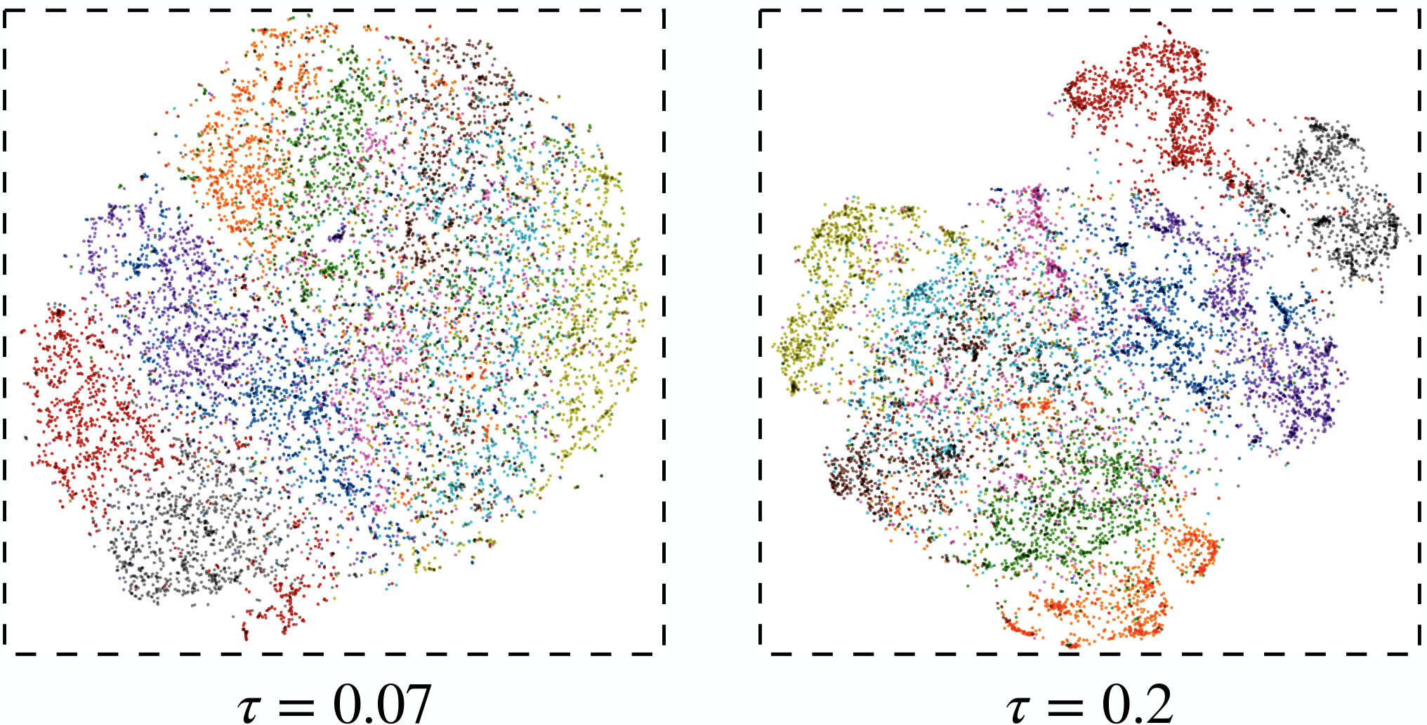
Overall, the contributions can be summarized as follows:
- •
We analyze the behaviours of the contrastive loss and show that contrastive loss is a hardness-aware loss. We validate that the hardness-aware property is significant to the success of contrastive loss.
- •
With a gradient analysis, we show that the temperature is a key parameter to control the strength of penalties on hard negative samples. Quantitative and qualitative experiments are conducted to validate the perspective.
- •
We show that there exists a uniformity-tolerance dilemma in contrastive learning, a good choice of temperature can compromise the two properties and improve the feature quality remarkably.
2 Related Work
Unsupervised learning methods have achieved great progress. Previous works focus on the design of novel pretext tasks, such as context prediction [7], jigsaw puzzle [19], colorization [34, 17], rotation [8], context encoder [21], split brain [35], deep cluster [2, 3] etc. The core idea of the above self-supervised methods is to capture some common priors between the pretext task and the downstream tasks. They assume that finishing the well-designed pretext tasks requires knowledge useful for downstream tasks such as classification [16], detection [9, 23], segmentation [24, 11] etc. Recently, unsupervised methods based on contrastive learning have drawn increasing attentions due to the excellent performances. Wu et al [33] propose an instance discrimination method, which first incorporates a contrastive loss (called NCE loss) to help discriminate different instances. CPC [20, 13] tries to learn context-invariant representations, and give a perspective of maximizing mutual information between different levels of features. CMC [27] is proposed to learn representations by maximizing the mutual information between different color channel views. SimCLR [4] simplifies the contrastive learning by only using different augmentations as different views, and tries to maximize the agreement between views. Besides, some methods try to maximize the agreement between different instances which may share similar semantic contents to learn instance-invariant representations, such as nearest neighbours discovery [14], local aggregation [37], invariance propagation [30], etc. On the other hand, contrastive loss requires many negative samples to help boost the performances. Instance discrimination [33] first proposes to use a memory bank to save the calculated features as the exponential moving average of the historical features. MoCo [10, 5] proposes to use a momentum queue to improve the consistency of the saved features.
There are also some works that try to understand the contrastive learning. Arora et al [25] present a theoretical framework for analyzing the contrastive learning by introducing latent classes and connect the relation between the unsupervised contrastive learning tasks and the downstream performances. Purushwalkam et al [22] try to demystify the unsupervised contrastive learning by focusing on the relation of data augmentation and the corresponding invariances. Tian et al [28] study the task-dependent optimal views of contrastive learning by a perspective of mutual information. Wu et al [32] give a systematical analysis to the relations between different contrastive learning methods and the corresponding forms of mutual information. Wang et al [31] try to understand the contrastive learning by two key properties, the alignment and uniformity. Different from the above works, we focus mainly on the inherent properties of the contrastive loss function. We emphasize the significance of the temperature , and use it as a proxy to analyze some intriguing phenomenons of the contrastive learning.
3 Hardness-aware Property
Given an unlabeled training set , the contrastive loss is formulated as:
| (1) |
where . is a feature extractor which maps the images from pixel space to a hypersphere space. is a function which can be same as [4], or comes from a memory bank [33], momentum queue [10], etc. For convenience, we define the probability of being recognized as as:
| (2) |
The contrastive loss tries to make the positive pairs attracted and the negative samples separated, i.e., the positive alignment and negative separation. This objective can also be achieved by using a more simple contrastive loss as:
| (3) |
However, we find that the above loss function performs much worse than the softmax-based contrastive loss of Eq 1. In the following parts, we will show that different with , the softmax-based contrastive loss is a hardness-aware loss function, which automatically concentrates on separating more informative negative samples to make the embedding distribution more uniform. Besides, we also find that the is a special case by approaching the temperature to . Next, we will start with a gradient analysis to explain the properties of the contrastive loss.
3.1 Gradients Analysis.
We analyze the gradients with respect to positive samples and different negative samples. We will show that the magnitude of positive gradient is equal to the sum of negative gradients. The temperature controls the distribution of negative gradients. Smaller temperature tends to concentrate more on the nearest neighbours of the anchor point, which plays a role in controlling the hardness-aware sensitivity. Specifically, the gradients with respect to the positive similarity and the negative similarity () are formulated as:
| (4) |
From Eq 4, we have the following observations: (1) The gradients with respect to negative samples is proportional to the exponential term , indicating that the contrastive loss is a hardness-aware loss function, which is different with the loss of Eq 3 that gives all negative similarities the same magnitude of gradients. (2) The magnitude of gradient with respect to positive sample is equal to the sum of gradients with respect to all negative samples, i.e., , which can define a probabilistic distribution to help understand the role of temperature .
3.2 The Role of temperature
The temperature plays a role in controlling the strength of penalties on hard negative samples. Specifically, we define , representing the relative penalty on negative sample . We have:
| (5) |
which obeys the Boltzman distribution. As the temperature decreases, the entropy of the distribution decreases strictly (the proof is in supplementary material). The distribution of becomes more sharp on the large similarity region, which gives large penalties to the samples closed to . Fig 3 shows the relation of and . From Fig 3, we observe that the relative penalty concentrates more on the high similarity region as the temperature decreases, and the relative penalty distribution tends to be more uniform as the temperature increases, which tends to give all negative samples the same magnitude of penalties. Besides, the effective penalty interval become narrowed as the temperature decreases. Extremely small temperatures will cause the contrastive loss only concentrate on the nearest one or two samples, which will heavily degenerate the performance. In this paper, we keep the temperatures in a reasonable interval to avoid this situation.
Let us consider two extreme cases: and . When , we have the following approximation:
| (6) | ||||
where is the maximum of the negative similarities. This shows that when the contrastive loss becomes a triplet loss with the margin of , which only focuses on the nearest negative sample. When , we approximate the contrastive learning as following:
| (7) | ||||
We use the Taylor expansion of and and omit the second or higher order infinitesimal terms. The above approximation of contrastive loss is equivalent to the simple contrastive loss , which shows that the simple contrastive loss is a special case of the softmax-based contrastive loss by approaching the temperature to .
We also conduct experiments to study the behaviours of the two extreme cases. Specifically, using the objective of Eq 6, the model can not learn any useful information. Using Eq 7 as the objective, the performances on downstream tasks are inferior to the models trained with the ordinary contrastive loss by a relative large margin. However, combining the loss of Eq 7 with an explicit hard negative sampling strategy, the model will achieve competitive downstream results, which shows the importance of the hardness-aware property of the contrastive loss.
3.3 Explicit Hard Negative Sampling
In this subsection, we study a more straightforward hard negative sampling strategy which truncates the gradients with respect to the uninformative negative samples. Specifically, given an upper quantile for the anchor sample , we define the informative interval as , and the uninformative interval as . We force the gradient ratio of which resides in the uninformative interval to 0, i.e., for , and the gradient ratio of residing in the informative interval as:
| (8) |
The above operation squeezes the negative gradients from the uninformative interval to the informative interval. The corresponding hard contrastive loss is:
| (9) |
The only penalizes the informative hard negative samples. The hard contrastive loss acts on hard negative samples in two ways: an explicit way that chooses the top nearest negative samples and an implicit way by the hardness-aware property. Using the same temperature with the contrastive loss of Eq 1, the hard contrastive loss usually generate more uniform embedding distribution, and it is beneficial to choose relative large temperatures. Besides, with this explicit hard negative sampling strategy, we show that the current popular contrastive loss of Eq 1 can be replaced by the simple form of Eq 3, with similar or even better performances on downstream tasks. Note that we are not the first to propose the idea of the above hard contrastive loss. LocalAggregation proposed by Zhuang et al[37] have used the above hard negative mining strategy. In this paper, we will concentrate on analyzing the behaviour of this contrastive loss.
4 Uniformity-Tolerance Dilemma
In this section, we study two properties: uniformity of the embedding distribution and the tolerance to semantically similar samples. The two properties are both important to the feature quality.
4.1 Embedding Uniformity
In [31], the authors find that the uniformity is a significant property in contrastive learning. The contrastive loss can be distangled to two parts, which encourages the positive features to be aligned and the embeddings to match a uniform distribution in a hypersphere. In this part, we will explore the relation between the local separation and the uniformity of embeddings. To this end, we incorporate the uniformity metric proposed by [31], which is based on a gaussian potential kernel:
| (10) |
We calculate on models trained with different temperatures to control different levels of local separation. We trained different models on CIFAR10, CIFAR100, SVHN and ImageNet100. Fig 4 shows the tendency. As the temperature increases, the embedding distribution tends to be less uniform (In Fig 4, the y-axis represents the ). And when is small, the embedding distribution is closer to a uniform distribution. This can be explained as follows: when the temperature is small, the contrastive loss tends to separate the positive samples close to the anchor sample, which makes the local distribution be sparse. With all samples are trained, the embedding space tends to make the neighbour of each point be sparse, and the distribution tends to be more uniform. For the hard contrastive loss, the situation is illustrated in Fig 6. With the hard contrastive loss as objective, the distribution tends to be more uniform. Besides, the uniformity keeps relative stable with the change of temperature compared with the ordinary contrastive loss. The explicit hard negative sampling weakened the effect of the temperature to control the hardness-aware property.
4.2 Tolerance to Potential Positive Samples
The objective of contrastive learning is to learn the augmentation alignment and instance discriminative embedding. The contrastive loss has no constraint to the distribution of the negative samples. However, with the help of heavy augmentation and strong abstraction ability of deep convolutional neural networks, the negative distribution reflects some extent of semantics, which is illustrated in Fig 1 (a). However, from the above section we have recognized that when the temperature is very small, the penalties to the nearest neighbours will be strengthened, which will push the semantically similar samples strongly to break the semantic structure of the embedding distribution. To explain the phenomenon in a quantitative manner, we measure the tolerance to the semantically consistent samples using the mean similarities of samples belong to the same class, which is formulated as:
| (11) |
where represents the supervised label of image . is an indicator function, having the value of 1 for and the value of 0 for . Fig 5 shows the tolerance with respect to different temperatures on CIFAR10 and CIFAR100. We could see that the tolerance is positively related to the temperature . However, the tolerance can not directly reflect the feature quality. For example, when all the samples reside in a single point of the hypersphere, then the tolerance is maximized, while the feature quality is bad. The tolerance reflects the local density of semantically related samples. An ideal model should be both locally clustered and globally uniform.
The contrastive loss meets a uniformity-tolerance dilemma. On the one hand, we hope to decrease the temperature to increase the uniformity of the embedding distribution, on the other hand, we hope to increase the temperature to make the embedding space tolerant to the similar samples. For the ordinary contrastive loss, it is a compromise to choose the appropriate temperature to balance both the embedding uniformity and the tolerance to semantically similar samples. The dilemma is caused by the inherent defect of unsupervised contrastive loss that it pushes all different instances ignoring their semantical relations.
Fig 6 and Fig 7 show the measurement of the embedding uniformity and the tolerance to samples in the same categories. We will see that the embedding distribution produced by hard contrastive loss is more uniform than the ordinary contrastive loss. This is caused by the increased gradients on the informative samples. Correspondingly, the tolerance to potential positive samples is decreased compared with the ordinary contrastive loss. However, the decrease of tolerance is caused by the increased uniformity, i.e., similarities with the samples in different categories are also decreased.
The hard contrastive loss deals better with the uniformity-tolerance dilemma. As we can see from Fig 6 and Fig 7, the uniformity keeps relative stable compared with the ordinary contrastive loss (from Fig 4). Relative large temperature can help be more tolerant to the potential positive samples without decreasing too much uniformity. We consider this is because the explicit hard negative sampling strategy is very effective for generating uniform embedding distribution.

5 Results
5.1 Experiment Details
Pretraining. We conduct experiments on CIFAR10, CIFAR100 [15], SVHN [18] and ImageNet100 [6]. The labels of the ImageNet100 are listed in the supplementary material. For the pretraining stage, we use resnet18 [12] with a minor modification (change the size of the first convolutional kernel as to adapt to input) as the backbone on CIFAR10, CIFAR100 and SVHN, and we use resnet50 [12] as the backbone on ImageNet100. For CIFAR10, CIFAR100 and SVHN, the augmentations follow [33]: a pixel crop is taken from a randomly resized image, and then undergoes random color jittering, random horizontal flip, and random gray scale conversion. For ImageNet-100, we follows [4] to add a random gaussian blur operation. To save the negative features, we follow [33] to create a memory bank which records the exponential moving average of the learned features. We use SGD as our optimizer. The SGD weight decay is 5e-4 for CIFAR10, CIFAR100 and SVHN, and 1e-4 for ImageNet100. The SGD momentum is set to 0.9. For the hard contrastive loss, the is set to 0.0819, 0.0819, 0.0315 and 0.034 for CIFAR10, CIFAR100, SVHN, and ImageNet100 (4095 negative samples). We train all models for 200 epochs with the learning rate multiplied by 0.1 at 160 and 190 epochs. We set an initial learning rate as 0.03, with a mini-batch size of 128.
Evaluation. We validate the performance of the pretrained models on linear classification models. Specifically, we train the linear layer for 100 epochs, with all convolutional layers frozen. We set an initial learning rate of 30.0, which is multiplied by 0.2 at 40, 60 and 80 epochs, and use SGD optimizer with weight decay of 0.
5.2 Local Separation
In this subsection, we evaluate the effect of the temperature. First, we try to figure out if the temperature accurately controls the strength of penalties on hard negative samples, furthermore, the extent of local separation. Specifically, we calculate for all point given an anchor sample , and then take an average over all anchor samples. We sort the similarities in a descending order and observe the distribution of the positive similarities and ten largest negative similarities that for all . We calculate these positive and negative similarities with the models trained on CIFAR100 and display them in Fig 8 (It is the same pattern when we calculate them on other datasets displayed in supplementary material). From Fig 8, we observe that: (1) As the decreases, the gap between positive samples and other confusing negative samples are larger, i.e., the positive and negative samples are more separable. (2) As increases, the positive similarities tend to be closer to 1. Observation (1) shows that small temperature indeed tends to push the hard negative samples more significantly, as indicated in the Fig 3, that small temperature makes the distribution of more sharply and concentrate most the penalties on the hardest negative samples (nearest neighbours). As the temperature increases, the positive samples and some confusing negative samples are likely to be less discriminative, and the relative penalties distribution tends to be more uniform to concentrate less on the hard negative samples. Observation (2) shows that as the temperature increases, the positive samples are more aligned, and the model tends to learn features more invariant to the data augmentations. We explain that the observation (2) is also caused by the role of temperature. For example, when the temperature is small, the contrastive loss punishes the hardest samples which are likely to share the similar content as the augmentations. Punishing these similar negative samples away significantly will make the objective of making positive samples alignment puzzling.
| Dataset | Result | Contrastive | Simple | HardContrastive | HardSimple | ||||||
|---|---|---|---|---|---|---|---|---|---|---|---|
| 0.07 | 0.3 | 0.7 | 1.0 | 0.07 | 0.3 | 0.7 | 1.0 | ||||
| CIFAR10 | accuracy | 79.75 | 83.27 | 82.69 | 82.21 | 74.83 | 79.2 | 83.63 | 84.19 | 84.19 | 84.84 |
| uniformity | 3.86 | 3.60 | 3.17 | 2.96 | 1.68 | 3.88 | 3.89 | 3.87 | 3.86 | 3.85 | |
| tolerance | 0.04 | 0.178 | 0.333 | 0.372 | 0.61 | 0.034 | 0.0267 | 0.030 | 0.030 | 0.030 | |
| CIFAR100 | accuracy | 51.82 | 56.44 | 50.99 | 48.33 | 39.31 | 50.77 | 56.55 | 57.54 | 56.77 | 55.71 |
| uniformity | 3.86 | 3.60 | 3.18 | 2.96 | 2.12 | 3.87 | 3.88 | 3.87 | 3.86 | 3.86 | |
| tolerance | 0.10 | 0.269 | 0.331 | 0.343 | 0.39 | 0.088 | 0.124 | 0.158 | 0.172 | 0.174 | |
| SVHN | accuracy | 92.55 | 95.47 | 94.17 | 92.07 | 70.83 | 91.82 | 94.79 | 95.02 | 95.26 | 94.99 |
| uniformity | 3.88 | 3.65 | 3.27 | 3.05 | 1.50 | 3.89 | 3.91 | 3.90 | 3.88 | 3.85 | |
| tolerance | 0.032 | 0.137 | 0.186 | 0.197 | 0.074 | 0.025 | 0.021 | 0.021 | 0.023 | 0.026 | |
| ImageNet100 | accuracy | 71.53 | 75.10 | 69.03 | 63.57 | 48.09 | 68.33 | 74.21 | 74.70 | 74.28 | 74.31 |
| uniformity | 3.917 | 3.693 | 3.323 | 3.08 | 1.742 | 3.929 | 3.932 | 3.927 | 3.923 | 3.917 | |
| tolerance | 0.093 | 0.380 | 0.427 | 0.456 | 0.528 | 0.067 | 0.096 | 0.121 | 0.134 | 0.157 | |
5.3 Feature Quality
We evaluate the performance of the contrastive models with different settings on cifar10, cifar100, SVHN and ImageNet100. Fig 9 shows the performances of linear classification on the four datasets respectively. For the models trained with ordinary contrastive loss (Eq 1), the performance tends to present a reverse-U shape. The models achieve the best performance when the temperature is 0.2 or 0.3. Models with small or large temperature achieve suboptimal performances. The results indicate that it is a compromise between uniformity and the tolerance. Models with small temperature tend to generate uniform embedding distribution, while they break the underlying semantic structure because they give large magnitudes of penalties to the closeness of potential positive samples. It is harmful to concentrate on the hardest negative samples due to they are very likely to be the samples whose semantic properties are very similar to the anchor point. On the other hand, models with large temperature tends to be more tolerant to the semantically consistent samples, while they may generate embeddings with not enough uniformity. Table 1 shows the numerical results, from which we can see that although the tolerance increases as the temperature increases, the uniformity decreases. This indicates that the embeddings tend to reside in a crowd region on the hypersphere. For the models trained with the hard contrastive loss (Eq 9), the above uniformity-tolerance dilemma is alleviated. From Fig 9, we observe that the models trained with hard contrastive loss achieve better results when the temperatures are large enough. This is because the uniformity is guaranteed by the explicit hard negative mining, which is reflected in Fig 6.
5.4 Uniformity and Tolerance
To measure the uniformity of embedding distribution and the tolerance to the semantically similar samples, we use Eq 10 and 11 as the measurement of those two properties. The experiments are conducted on CIFAR10, CIFAR100, SVHN and ImageNet100 respectively. Fig 4 and Fig 5 show the uniformity and tolerance of models trained with ordinary contrastive loss. Fig 6 and Fig 7 show the uniformity and tolerance of models trained with the hard contrastive loss. Detailed analysis is presented in Section 4. Concrete numerical values are present in Table 1 for some representative models, all results are listed in supplementary material.
5.5 Substitution of Contrastive Loss
We have claimed that the hardness-aware property is a key property to the success of contrastive loss. In this part, we will show that with explicit hard negative sampling strategy, the softmax-based contrastive loss of Eq 1 is not necessary, and a simple contrastive loss of Eq 3 works pretty well and achieve competitive results. Table 1 shows the results. Concretely, we use the simple contrastive loss of Eq 3 as objective, which is equivalent to the extreme case as approaches , and is marked as Simple in Table 1. Besides, we also trained models with a hard simple contrastive loss, using the nearest 4095 features as negative samples, which is marked as HardSimple in Table 1. Without the hardness-aware property, the learned models with perform much worse than models trained with ordinary contrastive loss (74.83 vs 83.27 on CIFAR10, 39.31 vs 56.44 on CIFAR100, 70.83 vs 95.47 on SVHN, 48.09 vs 75.10 on ImageNet100). However, when the negative samples of the are drawn from the nearest neighbours, the trained models achieve competitive results on all three datasets. This shows that the hardness-aware property is the core to the success of the contrastive loss.
6 Conclusion
In this paper, we try to understand the behaviour of the unsupervised contrastive loss. We show that the contrastive loss is a hardness-aware loss function, and the hardness-aware property is significant to the success of the contrastive loss. Besides, the temperature plays a key role in controlling the local separation and global uniformity of the embedding distributions. With the temperature as a proxy, we have studied the uniformity-tolerance dilemma, which is a challenge met by the unsupervised contrastive learning. We believe the uniformity-tolerance dilemma can be addressed by explicitly modeling the relation between different instances. We hope our work can inspire researchers to explore such algorithm to address the uniformity-tolerance dilemma.
7 Acknowledgments
This work was supported in part by the National Natural Science Foundation Project under Grant 62025304 and in part by the Seed Fund of Tsinghua University (Department of Computer Science and Technology)-Siemens Ltd., China Joint Research Center for Industrial Intelligence and Internet of Things.
References
- [1] Philip Bachman, R Devon Hjelm, and William Buchwalter. Learning representations by maximizing mutual information across views. arXiv preprint arXiv:1906.00910, 2019.
- [2] Mathilde Caron, Piotr Bojanowski, Armand Joulin, and Matthijs Douze. Deep clustering for unsupervised learning of visual features. In The European Conference on Computer Vision (ECCV), September 2018.
- [3] Mathilde Caron, Piotr Bojanowski, Julien Mairal, and Armand Joulin. Unsupervised pre-training of image features on non-curated data. In Proceedings of the IEEE International Conference on Computer Vision, pages 2959–2968, 2019.
- [4] Ting Chen, Simon Kornblith, Mohammad Norouzi, and Geoffrey Hinton. A simple framework for contrastive learning of visual representations. arXiv preprint arXiv:2002.05709, 2020.
- [5] Xinlei Chen, Haoqi Fan, Ross Girshick, and Kaiming He. Improved baselines with momentum contrastive learning. arXiv preprint arXiv:2003.04297, 2020.
- [6] Jia Deng, Wei Dong, Richard Socher, Li-Jia Li, Kai Li, and Li Fei-Fei. Imagenet: A large-scale hierarchical image database. In 2009 IEEE conference on computer vision and pattern recognition, pages 248–255. Ieee, 2009.
- [7] Carl Doersch, Abhinav Gupta, and Alexei A Efros. Unsupervised visual representation learning by context prediction. In Proceedings of the IEEE International Conference on Computer Vision, pages 1422–1430, 2015.
- [8] Spyros Gidaris, Praveer Singh, and Nikos Komodakis. Unsupervised representation learning by predicting image rotations. arXiv preprint arXiv:1803.07728, 2018.
- [9] Ross Girshick. Fast r-cnn. In Proceedings of the IEEE international conference on computer vision, pages 1440–1448, 2015.
- [10] Kaiming He, Haoqi Fan, Yuxin Wu, Saining Xie, and Ross Girshick. Momentum contrast for unsupervised visual representation learning. arXiv preprint arXiv:1911.05722, 2019.
- [11] Kaiming He, Georgia Gkioxari, Piotr Dollár, and Ross Girshick. Mask r-cnn. In Proceedings of the IEEE international conference on computer vision, pages 2961–2969, 2017.
- [12] Kaiming He, Xiangyu Zhang, Shaoqing Ren, and Jian Sun. Deep residual learning for image recognition. In Proceedings of the IEEE conference on computer vision and pattern recognition, pages 770–778, 2016.
- [13] Olivier J Hénaff, Aravind Srinivas, Jeffrey De Fauw, Ali Razavi, Carl Doersch, SM Eslami, and Aaron van den Oord. Data-efficient image recognition with contrastive predictive coding. arXiv preprint arXiv:1905.09272, 2019.
- [14] Jiabo Huang, Qi Dong, Shaogang Gong, and Xiatian Zhu. Unsupervised deep learning by neighbourhood discovery. In International Conference on Machine Learning, pages 2849–2858, 2019.
- [15] Alex Krizhevsky. Learning multiple layers of features from tiny images. 2009.
- [16] Alex Krizhevsky, Ilya Sutskever, and Geoffrey E Hinton. Imagenet classification with deep convolutional neural networks. In Advances in neural information processing systems, pages 1097–1105, 2012.
- [17] Gustav Larsson, Michael Maire, and Gregory Shakhnarovich. Learning representations for automatic colorization. In European Conference on Computer Vision, pages 577–593. Springer, 2016.
- [18] Yuval Netzer, Tao Wang, Adam Coates, Alessandro Bissacco, Bo Wu, and Andrew Y Ng. Reading digits in natural images with unsupervised feature learning. 2011.
- [19] Mehdi Noroozi and Paolo Favaro. Unsupervised learning of visual representations by solving jigsaw puzzles. In European Conference on Computer Vision, pages 69–84. Springer, 2016.
- [20] Aaron van den Oord, Yazhe Li, and Oriol Vinyals. Representation learning with contrastive predictive coding. arXiv preprint arXiv:1807.03748, 2018.
- [21] Deepak Pathak, Philipp Krahenbuhl, Jeff Donahue, Trevor Darrell, and Alexei A Efros. Context encoders: Feature learning by inpainting. In Proceedings of the IEEE conference on computer vision and pattern recognition, pages 2536–2544, 2016.
- [22] Senthil Purushwalkam Shiva Prakash and Abhinav Gupta. Demystifying contrastive self-supervised learning: Invariances, augmentations and dataset biases. Advances in Neural Information Processing Systems, 33, 2020.
- [23] Shaoqing Ren, Kaiming He, Ross Girshick, and Jian Sun. Faster r-cnn: Towards real-time object detection with region proposal networks. In Advances in neural information processing systems, pages 91–99, 2015.
- [24] Olaf Ronneberger, Philipp Fischer, and Thomas Brox. U-net: Convolutional networks for biomedical image segmentation. In International Conference on Medical image computing and computer-assisted intervention, pages 234–241. Springer, 2015.
- [25] Nikunj Saunshi, Orestis Plevrakis, Sanjeev Arora, Mikhail Khodak, and Hrishikesh Khandeparkar. A theoretical analysis of contrastive unsupervised representation learning. In International Conference on Machine Learning, pages 5628–5637, 2019.
- [26] Karen Simonyan and Andrew Zisserman. Very deep convolutional networks for large-scale image recognition. arXiv preprint arXiv:1409.1556, 2014.
- [27] Yonglong Tian, Dilip Krishnan, and Phillip Isola. Contrastive multiview coding. arXiv preprint arXiv:1906.05849, 2019.
- [28] Yonglong Tian, Chen Sun, Ben Poole, Dilip Krishnan, Cordelia Schmid, and Phillip Isola. What makes for good views for contrastive learning. arXiv preprint arXiv:2005.10243, 2020.
- [29] Laurens van der Maaten and Geoffrey E. Hinton. Visualizing data using t-sne. 2008.
- [30] Feng Wang, Huaping Liu, Di Guo, and Sun Fuchun. Unsupervised representation learning by invariance propagation. Advances in Neural Information Processing Systems, 33, 2020.
- [31] Tongzhou Wang and Phillip Isola. Understanding contrastive representation learning through alignment and uniformity on the hypersphere. arXiv preprint arXiv:2005.10242, 2020.
- [32] Mike Wu, Chengxu Zhuang, Milan Mosse, Daniel Yamins, and Noah Goodman. On mutual information in contrastive learning for visual representations. arXiv preprint arXiv:2005.13149, 2020.
- [33] Zhirong Wu, Yuanjun Xiong, Stella X Yu, and Dahua Lin. Unsupervised feature learning via non-parametric instance discrimination. In Proceedings of the IEEE Conference on Computer Vision and Pattern Recognition, pages 3733–3742, 2018.
- [34] Richard Zhang, Phillip Isola, and Alexei A Efros. Colorful image colorization. In European conference on computer vision, pages 649–666. Springer, 2016.
- [35] Richard Zhang, Phillip Isola, and Alexei A Efros. Split-brain autoencoders: Unsupervised learning by cross-channel prediction. In Proceedings of the IEEE Conference on Computer Vision and Pattern Recognition, pages 1058–1067, 2017.
- [36] Bolei Zhou, Agata Lapedriza, Jianxiong Xiao, Antonio Torralba, and Aude Oliva. Learning deep features for scene recognition using places database. In Advances in neural information processing systems, pages 487–495, 2014.
- [37] Chengxu Zhuang, Alex Lin Zhai, and Daniel Yamins. Local aggregation for unsupervised learning of visual embeddings. In Proceedings of the IEEE International Conference on Computer Vision, pages 6002–6012, 2019.