跳到论文正文
W Papers独立论文阅读器 arXiv:2012.09623 论文正文 计算阅读时间 · 0%
引用这篇论文根据当前论文元数据生成,正式投稿前建议核对。


License: arXiv.org perpetual non-exclusive license
arXiv:2012.09623v1 [math.ST] 17 Dec 2020

A geometric investigation into the tail dependence of vine copulas
Emma S. Simpson, Jennifer L. Wadsworth and Jonathan A. Tawn
Lancaster University

Keywords: coefficient of tail dependence; gauge function; multivariate extremes; vine copula.

Abstract

Vine copulas are a type of multivariate dependence model, composed of a collection of bivariate copulas that are combined according to a specific underlying graphical structure. Their flexibility and practicality in moderate and high dimensions have contributed to the popularity of vine copulas, but relatively little attention has been paid to their extremal properties. To address this issue, we present results on the tail dependence properties of some of the most widely studied vine copula classes. We focus our study on the coefficient of tail dependence and the asymptotic shape of the sample cloud, which we calculate using the geometric approach of Nolde, 2014. We offer new insights by presenting results for trivariate vine copulas constructed from asymptotically dependent and asymptotically independent bivariate copulas, focusing on bivariate extreme value and inverted extreme value copulas, with additional detail provided for logistic and inverted logistic examples. We also present new theory for a class of higher dimensional vine copulas, constructed from bivariate inverted extreme value copulas.

1 Introduction

In multivariate extreme value analysis, the tail dependence properties of variables are an important consideration for model selection. In particular, one may be interested in whether or not they exhibit so-called asymptotic dependence, where the largest values can occur simultaneously across all variables; see Coles et al., 1999. Suppose we are interested in a model for the dd random variables 𝑿=(X1,…,Xd)\bm{X}=(X_{1},\ldots,X_{d}), which we assume have standard exponential margins to focus only on dependence, i.e., Pr⁡(Xi<x)=1−e−x\Pr(X_{i}<x)=1-e^{-x}, x≥0x\geq 0, for i=1,…,di=1,\ldots,d. For any subset of these variables, 𝑿𝒞=(Xi:i∈𝒞)\bm{X}_{\mathcal{C}}=(X_{i}:i\in\mathcal{C}), with 𝒞⊆𝒟={1,…,d}\mathcal{C}\subseteq\mathcal{D}=\{1,\ldots,d\} and |𝒞|≥2|\mathcal{C}|\geq 2, and any j∈𝒞j\in\mathcal{C}, one can consider the measure

χ𝒞=limu→∞Pr⁡(Xi>u,i∈𝒞)Pr⁡(Xj>u)=limu→∞eu​Pr⁡(Xi>u,i∈𝒞),\displaystyle\chi_{\mathcal{C}}=\lim_{u\rightarrow\infty}\frac{\Pr\left(X_{i}>u;i\in\mathcal{C}\right)}{\Pr(X_{j}>u)}=\lim_{u\rightarrow\infty}e^{u}\Pr\left(X_{i}>u;i\in\mathcal{C}\right), (1)

which corresponds to the limiting probability that all variables are above some high threshold uu, given that any one of the variables exceeds uu. If χ𝒞>0\chi_{\mathcal{C}}>0, all variables in 𝑿𝒞\bm{X}_{\mathcal{C}} exhibit asymptotic dependence, while χ𝒞=0\chi_{\mathcal{C}}=0 means that not all variables in 𝑿𝒞\bm{X}_{\mathcal{C}} can be simultaneously large. In the latter case, if |𝒞|=2|\mathcal{C}|=2, the two variables cannot be simultaneously extreme, and are said to exhibit asymptotic independence; if |𝒞|>2|\mathcal{C}|>2, it is still possible to have χ𝒞~>0\chi_{\tilde{\mathcal{C}}}>0 for any 𝒞~⊂𝒞\tilde{\mathcal{C}}\subset\mathcal{C}. That is, variables indexed by 𝒞~\tilde{\mathcal{C}} could take their largest values simultaneously while at least one of those indexed by 𝒞∖𝒞~\mathcal{C}\setminus\tilde{\mathcal{C}} are of smaller order. The collection of all sets of variables which can or cannot be simultaneously extreme corresponds to a more complicated extremal dependence structure; see Goix et al., 2017 or Simpson et al., 2020.

Moreover, if χ𝒞=0\chi_{\mathcal{C}}=0, there could be some sub-asymptotic dependence between 𝑿𝒞\bm{X}_{\mathcal{C}}, despite the lack of asymptotic dependence in the limit, and the measure χ𝒞\chi_{\mathcal{C}} does not tell the full story. To investigate this behaviour further, it is common to consider the coefficient of tail dependence, introduced by Ledford and Tawn, 1996. Again for a subset of exponential variables 𝑿𝒞\bm{X}_{\mathcal{C}}, with |𝒞|≥2|\mathcal{C}|\geq 2, this is defined via the relation

Pr(Xi>x:i∈𝒞)∼L𝒞(ex)e−x/η𝒞,\displaystyle\Pr\left(X_{i}>x:i\in\mathcal{C}\right)\sim L_{\mathcal{C}}(e^{x})e^{-x/\eta_{\mathcal{C}}}, (2)

as x→∞x\rightarrow\infty, where L𝒞L_{\mathcal{C}} denotes a function that is slowly varying at infinity, and η𝒞∈(0,1]\eta_{\mathcal{C}}\in(0,1]. If η𝒞=1\eta_{\mathcal{C}}=1 and L𝒞​(x)↛0L_{\mathcal{C}}(x)\not\rightarrow 0, as x→∞x\rightarrow\infty, the variables in 𝑿𝒞\bm{X}_{\mathcal{C}} are asymptotically dependent. For η𝒞<1\eta_{\mathcal{C}}<1, these variables cannot be simultaneously large, and the value of the coefficient quantifies the strength of sub-asymptotic dependence between the variables. The set of measures {χ𝒞,η𝒞:𝒞⊆𝒟,|𝒞|≥2}\{\chi_{\mathcal{C}},\eta_{\mathcal{C}}:\mathcal{C}\subseteq\mathcal{D},|\mathcal{C}|\geq 2\} therefore provide a summary of the key extremal dependence features of 𝑿\bm{X}.

Often, the value of η𝒞\eta_{\mathcal{C}} can be calculated directly from (2) for a given model, but in some cases, only the joint density of 𝑿𝒞\bm{X}_{\mathcal{C}} can be specified in closed form, and not the required joint survivor function. Nolde, 2014 presents a strategy to overcome this issue, based on the geometry of scaled random samples from the joint distribution of 𝑿𝒞\bm{X}_{\mathcal{C}}. A simplified version of the approach of Nolde, 2014, which we discuss further in Section 2.1, assumes standard exponential margins, and joint density f𝒞​(𝒙𝒞)f_{\mathcal{C}}(\bm{x}_{\mathcal{C}}), with the idea being to study the gauge function g𝒞​(𝒙𝒞)g_{\mathcal{C}}(\bm{x}_{\mathcal{C}}) such that

−ln⁡f𝒞​(t​𝒙𝒞)∼t​g𝒞​(𝒙𝒞),\displaystyle-\ln f_{\mathcal{C}}(t\bm{x}_{\mathcal{C}})\sim tg_{\mathcal{C}}(\bm{x}_{\mathcal{C}}), (3)

as t→∞t\rightarrow\infty, with g𝒞​(𝒙𝒞)g_{\mathcal{C}}(\bm{x}_{\mathcal{C}}) being homogeneous of order 1. The limiting shape of suitably scaled samples from 𝑿𝒞\bm{X}_{\mathcal{C}} is described by the set of points where the gauge function is at most one, i.e., {𝒙𝒞:g𝒞​(𝒙𝒞)≤1}\{\bm{x}_{\mathcal{C}}:g_{\mathcal{C}}(\bm{x}_{\mathcal{C}})\leq 1\}, and studying this set can reveal the value of η𝒞\eta_{\mathcal{C}} and provide insight into other aspects of the extremal dependence structure; see Nolde and Wadsworth, 2020. We present some example gauge function calculations in Section 2.3 for the case where |𝒞|=2|\mathcal{C}|=2, for both asymptotically dependent and asymptotically independent models, and demonstrate how they can be used to obtain η𝒞\eta_{\mathcal{C}}.

One drawback of this method is that it is only applicable when the joint density of 𝑿𝒞\bm{X}_{\mathcal{C}} can be obtained analytically. It may be the case that we have a closed form joint density for variables 𝑿\bm{X}, but not for all 𝑿𝒞\bm{X}_{\mathcal{C}} with 𝒞⊂𝒟\mathcal{C}\subset\mathcal{D}. Nolde and Wadsworth, 2020 show how to derive lower-dimensional gauge functions from higher-dimensional ones, and in Section 2, we review this technique for the calculation of g𝒞​(𝒙𝒞)g_{\mathcal{C}}(\bm{x}_{\mathcal{C}}) and η𝒞\eta_{\mathcal{C}} in such cases. In our study of vine copulas, which have dimension d≥3d\geq 3, this approach can be necessary to obtain even some bivariate results.

In this paper, we focus on investigating the tail behaviour of vine copulas. These models exploit the wide range of existing parametric bivariate copula models to create parametric copula models for higher dimensions, where there are fewer options available. This allows for the construction of flexible models with the possibility of capturing a wide range of dependence features. The idea of combining bivariate copulas in this way was first proposed by Joe, 1996; developed further by Bedford and Cooke, 2001; Bedford and Cooke, 2002, who proposed the use of a type of graphical model called vines to aid the modelling procedure; and further studied in an inferential context by Aas et al., 2009. A textbook treatment of these models is provided by Kurowicka and Joe, 2010. We give an introduction to vine copula modelling in Section 3. Vine copulas are widely used in financial applications; a summary of these applications is provided by Aas, 2016, with examples including Brechmann et al., 2012 and Dißmann et al., 2013.

Vine copulas reduce model formulation to a series of pairwise copula selections, and therefore appear to be ideal for modelling extremal dependence since, as noted earlier, such dependence is known to have complex structure. For vine copulas over variables indexed by 𝒟\mathcal{D}, Joe et al., 2010 have made major progress in deriving general results about χ𝒟\chi_{\mathcal{D}}, defined in (1), for any vine copula. In particular, they have determined some relationships of χ𝒟\chi_{\mathcal{D}} with the values of χ𝒞\chi_{\mathcal{C}} (for |𝒞|=2|\mathcal{C}|=2) associated with the bivariate copulas used in the vine construction. Primarily, they consider the case where all pairwise χ𝒞\chi_{\mathcal{C}} are non-zero, and therefore focus only on asymptotically dependent copulas. They also study the result of imposing asymptotic independence or asymptotic dependence in certain pair copulas, and how this leads to constraints on χ𝒟\chi_{\mathcal{D}}.

Some pairwise copulas have χ𝒞=0\chi_{\mathcal{C}}=0, with a range of examples given by Heffernan, 2000. Particularly noteworthy cases include the pairwise Gaussian copula and the Morgernstern copula (see Example 2.1 of Joe et al., 2010), with parameters −1<ρ<1-1<\rho<1 and −1<θ<1-1<\theta<1, respectively. For vine copulas, when some of the pairwise χ𝒞=0\chi_{\mathcal{C}}=0, the results of Joe et al., 2010 only give that χ𝒟=0\chi_{\mathcal{D}}=0, and they fail to give any information about the dependence in the joint tail of variables, e.g., the probability that all of the variables are simultaneously large. In that case we are interested in the numerator of (1) (prior to it being taken to its limit for χ𝒟\chi_{\mathcal{D}}). When χ𝒟=0\chi_{\mathcal{D}}=0, all we know is that this joint probability is smaller order than the marginal probability of one of the variables being large (as in the denominator of (1)). Such joint tail probabilities are important in characterising the tail, and for assessing risk in applications (Coles and Tawn, 1994; Heffernan and Tawn, 2004).

The tail parameter η𝒞\eta_{\mathcal{C}} for all 𝒞⊆𝒟\mathcal{C}\subseteq\mathcal{D} in (2) is important, as it captures the level of asymptotic independence, with η𝒞=1\eta_{\mathcal{C}}=1 corresponding to asymptotic dependence (for all cases where χ𝒞>0\chi_{\mathcal{C}}>0) and 0<η𝒞<10<\eta_{\mathcal{C}}<1 corresponding to levels of asymptotic independence. For example, for the bivariate Gaussian copula, η{1,2}=(1+ρ)/2\eta_{\{1,2\}}=(1+\rho)/2 (with −1<ρ<1-1<\rho<1 denoting the usual “correlation coefficient”), and for the Morgenstern copula, η{1,2}=1/2\eta_{\{1,2\}}=1/2 for all θ\theta. So, although these two copulas have identical χ{1,2}\chi_{\{1,2\}} values, they have different values of η{1,2}\eta_{\{1,2\}} unless ρ=0\rho=0.

Our paper therefore differs from Joe et al., 2010 in that we aim to find η𝒞\eta_{\mathcal{C}} in cases where their results simply give χ𝒞=0\chi_{\mathcal{C}}=0, for all 𝒞⊆𝒟\mathcal{C}\subseteq\mathcal{D}. With this, we seek to better understand how the bivariate copulas and underlying graphical structure used in the construction of a vine copula affect these additional extremal dependence features of the variables, and to be the first to study the gauge function for vine copulas.

Throughout this paper, we consider exponential marginal distributions, but allow a variety of different bivariate copulas to be used in the vine copula construction. If only bivariate Gaussian copulas are used in this construction, the overall joint distribution of the variables will also be Gaussian (Joe, 1996; Joe et al., 2010). Since the tail dependence features of the Gaussian model are well-studied in the literature, we focus on cases where the pair copulas are from extreme value or inverted extreme value classes of distributions (Ledford and Tawn, 1997; Papastathopoulos and Tawn, 2016). These classes are widely studied in the extreme value literature; while they are not in themselves parametric distributions, they do include a range of well-known parametric examples (Coles and Tawn, 1991; Cooley et al., 2010; Ballani and Schlather, 2011). Bivariate extreme value distributions exhibit asymptotic dependence, while their inverted counterparts exhibit asymptotic independence. Studying these two classes is therefore sufficient to reveal a rich variety of structures within the vine copula framework.

Vine copula models provide an example of when the joint distribution function of the variables generally cannot be calculated analytically. Moreover, the joint densities corresponding to certain subsets of the variables often do not have closed forms. To study the tail behaviour of these models, we calculate η𝒞\eta_{\mathcal{C}} for several examples, through the application of the geometric approach of Nolde, 2014. Our investigation reveals interesting features of the shape of the gauge function in (3) for vine copula models.

Having introduced the geometric methodology for studying extremal dependence in Section 2, and provided an overview of vine copula modelling in Section 3, the remainder of the paper is structured as follows. In Section 4, we present calculations and results for cases where each pair copula is from the inverted extreme value family of distributions. In higher than three dimensions, the underlying graphical structure of the copula is a further consideration, and we also present results for inverted extreme value pair copulas here, with two different types of underlying vine structure. In the trivariate and higher-dimensional examples, we present results for inverted logistic examples as a special case. In Section 5, we return to the trivariate case, presenting results for vine copulas constructed from combinations of extreme value and inverted extreme value pair copulas.

2 Geometric approaches for calculating η𝒞\eta_{\mathcal{C}}

2.1 The geometric approach of Nolde, 2014

Nolde, 2014 proposes a method to calculate the coefficient of tail dependence η𝒞\eta_{\mathcal{C}} based on the shape of scaled random samples from the vector 𝑿𝒞\bm{X}_{\mathcal{C}}. This follows earlier work by Balkema and Nolde, 2010, who showed that the limiting shape of the sample cloud could be used to determine the presence of asymptotic independence. Theorem 2.1 of Nolde, 2014 provides the result for marginal distributions with Weibull-type tails. We take a simplified approach by focusing on the special case where all margins have standard exponential distributions, which is possible without losing information about the extremal dependence properties of the variables.

Interest lies with the gauge function g𝒞​(𝒙𝒞)g_{\mathcal{C}}(\bm{x}_{\mathcal{C}}), satisfying equation (3). In this case, we consider the scaled random sample (𝑿𝒞,1/ln⁡n,…,𝑿𝒞,n/ln⁡n)\left(\bm{X}_{\mathcal{C},1}/\ln n,\ldots,\bm{X}_{\mathcal{C},n}/\ln n\right), as n→∞n\rightarrow\infty, with the scaling function ln⁡n\ln n chosen due to the exponential margins. The sample cloud converges onto the compact set G𝒞∗={𝒙𝒞∈ℝ|𝒞|:g𝒞​(𝒙𝒞)≤1}⊆[0,1]|𝒞|G^{*}_{\mathcal{C}}=\{\bm{x}_{\mathcal{C}}\in\mathbb{R}^{|\mathcal{C}|}:g_{\mathcal{C}}(\bm{x}_{\mathcal{C}})\leq 1\}\subseteq[0,1]^{|\mathcal{C}|}, which also has the property of being star-shaped, i.e., if 𝒙𝒞∈G𝒞∗\bm{x}_{\mathcal{C}}\in G^{*}_{\mathcal{C}}, then t​𝒙𝒞∈G𝒞∗t\bm{x}_{\mathcal{C}}\in G^{*}_{\mathcal{C}} for all t∈(0,1)t\in(0,1). We denote the part of the boundary of this set where the gauge function equals one by G𝒞={𝒙𝒞∈ℝ|𝒞|:g𝒞​(𝒙𝒞)=1}⊂G𝒞∗⊆[0,1]|𝒞|G_{\mathcal{C}}=\{\bm{x}_{\mathcal{C}}\in\mathbb{R}^{|\mathcal{C}|}:g_{\mathcal{C}}(\bm{x}_{\mathcal{C}})=1\}\subset G^{*}_{\mathcal{C}}\subseteq[0,1]^{|\mathcal{C}|}.

Nolde, 2014 shows that the coefficient of tail dependence can be calculated as

η𝒞=min{r:G𝒞∩[r,∞)|𝒞|≠∅},\displaystyle\eta_{\mathcal{C}}=\min\left\{r:G_{\mathcal{C}}\cap[r,\infty)^{|\mathcal{C}|}\neq\emptyset\right\}, (4)

which Nolde and Wadsworth, 2020 show is equivalent to

η𝒞={min𝒙𝒞:min⁡(𝒙𝒞)=1g𝒞(𝒙𝒞)}−1={min𝒙𝒞:min⁡(𝒙𝒞)≥1g𝒞(𝒙𝒞)}−1.\displaystyle\eta_{\mathcal{C}}=\left\{\min\limits_{\bm{x}_{\mathcal{C}}:\min(\bm{x}_{\mathcal{C}})=1}g_{\mathcal{C}}\left(\bm{x}_{\mathcal{C}}\right)\right\}^{-1}=\left\{\min\limits_{\bm{x}_{\mathcal{C}}:\min(\bm{x}_{\mathcal{C}})\geq 1}g_{\mathcal{C}}\left(\bm{x}_{\mathcal{C}}\right)\right\}^{-1}. (5)

The case where argmin𝒙𝒞:min⁡(𝒙𝒞)=1g𝒞(𝒙𝒞)=𝟏∈ℝ|𝒞|\arg\min_{\bm{x}_{\mathcal{C}}:\min(\bm{x}_{\mathcal{C}})=1}g_{\mathcal{C}}\left(\bm{x}_{\mathcal{C}}\right)=\bm{1}\in\mathbb{R}^{|\mathcal{C}|} occurs if and only if η𝒞=1/g𝒞​(𝟏)\eta_{\mathcal{C}}=1/g_{\mathcal{C}}(\bm{1}), corresponding to the intersection in (4) occurring when all variables are equal, i.e., when xj=xkx_{j}=x_{k} for all j,k∈𝒞j,k\in\mathcal{C}. We also note that the quantity 1/g𝒞​(𝟏)1/g_{\mathcal{C}}(\bm{1}) will always provide a lower bound for η𝒞\eta_{\mathcal{C}}, and if g𝒞​(𝟏)=1g_{\mathcal{C}}(\bm{1})=1, then it must be the case that η𝒞=1\eta_{\mathcal{C}}=1. When analytical minimisation of g𝒞g_{\mathcal{C}} is difficult or impossible, numerical investigation can be used to determine where the minimum occurs.

This numerical minimisation may be undertaken using optimisation software such as optim in R. Implementation is simpler using the second form in (5), i.e., with min⁡(𝒙𝒞)≥1\min(\bm{x}_{\mathcal{C}})\geq 1, and one can check that the numerical optimisation gives min⁡(𝒙𝒞)=1\min(\bm{x}_{\mathcal{C}})=1. It is advisable to compare results across a range of starting values of 𝒙𝒞\bm{x}_{\mathcal{C}} to ensure convergence. If convergence is not reached, an alternative is to carry out the investigation across the range of subspaces of interest, i.e., where different subsets of 𝒙𝒞\bm{x}_{\mathcal{C}} are equal to one, and to compare these results. While it is clearly preferable to use theoretical results, where this is not possible, this numerical approach can be useful. Moreover, where theoretical results are difficult to obtain, numerical studies may provide additional insight that can facilitate analytical calculations.

We subsequently drop the subscript 𝒞\mathcal{C} from the set G𝒞G_{\mathcal{C}}, density f𝒞f_{\mathcal{C}} and gauge function g𝒞g_{\mathcal{C}} when discussing the overall vector of variables 𝑿\bm{X}, i.e., when 𝒞=𝒟\mathcal{C}=\mathcal{D}.

2.2 Lower dimensional subsets

The method of Nolde, 2014 can only be used to calculate the coefficient η𝒞\eta_{\mathcal{C}} in cases where the density f𝒞​(𝒙𝒞)f_{\mathcal{C}}(\bm{x}_{\mathcal{C}}) can be obtained analytically. In some cases, including many vine copula examples, we may have the form of f⁡(𝒙)f(\bm{x}), but no closed form of f𝒞​(𝒙𝒞)f_{\mathcal{C}}(\bm{x}_{\mathcal{C}}) for certain subsets 𝒞⊂𝒟\mathcal{C}\subset\mathcal{D}, so the method cannot be directly applied to obtain η𝒞\eta_{\mathcal{C}}. Nolde and Wadsworth, 2020 use results on projections of sample clouds to show that the gauge function g𝒞​(𝒙𝒞)g_{\mathcal{C}}(\bm{x}_{\mathcal{C}}) can be obtained from the gauge function g⁡(𝒙)g(\bm{x}) for any set 𝒞⊂𝒟\mathcal{C}\subset\mathcal{D} with |𝒞|∈[1,d−1]|\mathcal{C}|\in[1,d-1], by

g𝒞(𝒙𝒞)=minxi:i∉𝒞g(𝒙).\displaystyle g_{\mathcal{C}}\left(\bm{x}_{\mathcal{C}}\right)=\min_{x_{i}:i\notin\mathcal{C}}g(\bm{x}). (6)

Once this gauge function has been obtained, the remainder of the procedure to calculate η𝒞\eta_{\mathcal{C}} continues as in Section 2.1. In particular, this implies that

η𝒞={min𝒙𝒞:min⁡(𝒙𝒞)≥1g𝒞(𝒙𝒞)}−1={min𝒙:min⁡{xi:i∈𝒞≥1}min⁡{xi:i∉𝒞≥0}g(𝒙)}−1.\displaystyle\eta_{\mathcal{C}}=\left\{\min\limits_{\bm{x}_{\mathcal{C}}:\min(\bm{x}_{\mathcal{C}})\geq 1}g_{\mathcal{C}}(\bm{x}_{\mathcal{C}})\right\}^{-1}=\left\{\min\limits_{\begin{subarray}{c}\bm{x}:\min\{x_{i}:i\in\mathcal{C}\geq 1\}\\ ~~\min\{x_{i}:i\notin\mathcal{C}\geq 0\}\end{subarray}}g(\bm{x})\right\}^{-1}. (7)

If the gauge function still cannot be obtained analytically via the minimisation in (6), numerical methods can again be exploited. Numerical calculation of η𝒞\eta_{\mathcal{C}} will require optimising equation (6) within equation (5), as in (7), and the result of this optimisation procedure may again be used to motivate the theoretical calculation of η𝒞\eta_{\mathcal{C}}. In Sections 4 and 5 we will study cases where we have the form of g{1,2,3}​(x1,x2,x3)g_{\{1,2,3\}}(x_{1},x_{2},x_{3}) and wish to deduce η{1,3}\eta_{\{1,3\}}, where the analytical form of g{1,3}​(x1,x3)g_{\{1,3\}}(x_{1},x_{3}) is not known. If theoretical arguments or numerical investigations suggest that the minimum in (5) occurs when x1=x3=1x_{1}=x_{3}=1, i.e., η{1,3}=1/g{1,3}​(1,1)\eta_{\{1,3\}}=1/g_{\{1,3\}}(1,1), one can focus solely on this case in (7). That is, only calculation of g{1,3}​(1,1)=minv⁡g⁡(1,v,1)g_{\{1,3\}}(1,1)=\min_{v}g(1,v,1) is needed, which may be possible even when the minimisation in (6) over the full range of (x1,x3)(x_{1},x_{3}) values is not. In addition, if we can find any 𝒙\bm{x} with xi≥1,i∈𝒞x_{i}\geq 1,i\in\mathcal{C} and xi≥0,i∉𝒞x_{i}\geq 0,i\notin\mathcal{C}, such that g⁡(𝒙)=1g(\bm{x})=1, then this must correspond to the required minimum, and η𝒞=1\eta_{\mathcal{C}}=1.

2.3 Bivariate examples

To demonstrate the geometric approach discussed in Section 2.1, we consider six bivariate examples, corresponding to three distributions belonging to each of the asymptotic independence and asymptotic dependence classes. We also comment on interesting features relating to the shape of the set GG in each case. In this section, we generally use plots to determine where the intersection in (4) occurs, but we note that equation (5) also holds in all cases.

We begin with the example of independent exponential variables, where it is straightforward to obtain the gauge function as g⁡(x1,x2)=x1+x2g(x_{1},x_{2})=x_{1}+x_{2}, i.e., the set GG corresponds to the straight line x2=1−x1x_{2}=1-x_{1} for x1,x2∈[0,1]x_{1},x_{2}\in[0,1]. This is demonstrated in case (i) of Fig. 1, and it is clear that the smallest value of rr such that GG and [r,∞)2[r,\infty)^{2} do not intersect yields η{1,2}=1/2\eta_{\{1,2\}}=1/2. In Fig. 1 we plot scaled samples of size 1000 from the various models; note that since the gauge function calculations are based on asymptotic results, some of this finite sample may lie outside the set GG.

As a second asymptotically independent model, we consider a bivariate Gaussian copula model having exponential margins and covariance matrix Σ\Sigma with Σ1,1=Σ2,2=1\Sigma_{1,1}=\Sigma_{2,2}=1 and Σ1,2=Σ2,1=ρ∈[0,1)\Sigma_{1,2}=\Sigma_{2,1}=\rho\in[0,1). Nolde, 2014 shows that this model has gauge function

g⁡(x1,x2)=(1−ρ2)−1​(x1+x2−2​ρ​x11/2​x21/2),g(x_{1},x_{2})=(1-\rho^{2})^{-1}\left(x_{1}+x_{2}-2\rho x_{1}^{1/2}x_{2}^{1/2}\right),

with x1,x2≥0x_{1},x_{2}\geq 0. This is demonstrated in case (ii) of Fig. 1 for ρ=0.5\rho=0.5. Minimisation as in (5) reveals that η{1,2}=1/g⁡(1,1)=(1+ρ)/2=0.75\eta_{\{1,2\}}=1/g(1,1)=(1+\rho)/2=0.75, corresponding to the known coefficient for a Gaussian model (Ledford and Tawn, 1996).

Examples (iii), (v) and (vi) are based on the class of bivariate extreme value distributions, which in exponential margins, have a joint distribution function written as

F⁡(x1,x2)=exp⁡[−V⁡{−1ln⁡(1−e−x1),−1ln⁡(1−e−x2)}],\displaystyle F(x_{1},x_{2})=\exp\left[-V\left\{\frac{-1}{\ln\left(1-e^{-x_{1}}\right)},\frac{-1}{\ln\left(1-e^{-x_{2}}\right)}\right\}\right], (8)

for x1,x2≥0x_{1},x_{2}\geq 0 and some exponent measure V⁡(x,y)V(x,y) that is homogeneous of order −1-1 and takes the form

V⁡(x,y)=2​∫01max⁡(wx,1−wy)​𝑑H​(w),\displaystyle V(x,y)=2\int_{0}^{1}\max\left(\frac{w}{x},\frac{1-w}{y}\right)dH(w), (9)

for x,y>0x,y>0, and spectral distribution HH satisfying the moment constraint ∫01w​𝑑H​(w)=1/2\int_{0}^{1}wdH(w)=1/2. We let V1V_{1}, V2V_{2} and V12V_{12} denote the derivatives of the exponent measure with respect to the first, second and both components, respectively, where these are assumed to exist. One example of a method belonging to this class is the logistic distribution, with exponent measure

V(x,y)=(x−1/α+y−1/α)α,for some α∈(0,1] and x,y>0,\displaystyle V(x,y)=\left(x^{-1/\alpha}+y^{-1/\alpha}\right)^{\alpha},~~~~\text{for some }\alpha\in(0,1]\text{ and }x,y>0, (10)

see Tawn, 1988. We return to the extreme value distribution in case (v), but first use these results to consider a final asymptotically independent model: the inverted bivariate extreme distribution. Models of this class are obtained by exchanging the upper and lower tail features in extreme value distribution (8). In exponential margins, the model has distribution function

F⁡(x1,x2)=1−e−x1−e−x2+exp⁡{−V⁡(x1−1,x2−1)},F(x_{1},x_{2})=1-e^{-x_{1}}-e^{-x_{2}}+\exp\left\{-V\left(x_{1}^{-1},x_{2}^{-1}\right)\right\},

for x1,x2≥0x_{1},x_{2}\geq 0. Differentiating with respect to both components to obtain the density f⁡(x1,x2)f(x_{1},x_{2}), we have

−ln⁡f⁡(t​x1,t​x2)=\displaystyle-\ln f(tx_{1},tx_{2})= 2​ln⁡(t​x1)+2​ln⁡(t​x2)+V⁡{(t​x1)−1,(t​x2)−1}\displaystyle 2\ln(tx_{1})+2\ln(tx_{2})+V\left\{(tx_{1})^{-1},(tx_{2})^{-1}\right\}
−ln⁡[V1​{(t​x1)−1,(t​x2)−1}​V2​{(t​x1)−1,(t​x2)−1}−V12​{(t​x1)−1,(t​x2)−1}]\displaystyle\hskip 28.45274pt-\ln\left[V_{1}\left\{(tx_{1})^{-1},(tx_{2})^{-1}\right\}V_{2}\left\{(tx_{1})^{-1},(tx_{2})^{-1}\right\}-V_{12}\left\{(tx_{1})^{-1},(tx_{2})^{-1}\right\}\right]
=\displaystyle= 2​ln⁡(t​x1)+2​ln⁡(t​x2)+t​V​(x1−1,x2−1)−ln⁡{t4​V1​(x1−1,x2−1)​V2​(x1−1,x2−1)−t3​V12​(x1−1,x2−1)}\displaystyle 2\ln(tx_{1})+2\ln(tx_{2})+tV\left(x_{1}^{-1},x_{2}^{-1}\right)-\ln\left\{t^{4}V_{1}\left(x_{1}^{-1},x_{2}^{-1}\right)V_{2}\left(x_{1}^{-1},x_{2}^{-1}\right)-t^{3}V_{12}\left(x_{1}^{-1},x_{2}^{-1}\right)\right\}
=\displaystyle= t​V​(x1−1,x2−1)+O⁡(ln⁡t),\displaystyle tV\left(x_{1}^{-1},x_{2}^{-1}\right)+O(\ln t), (11)

as t→∞t\rightarrow\infty, by exploiting the homogeneity of the exponent measure. That is, the gauge function is given by g⁡(x1,x2)=V⁡(x1−1,x2−1)g(x_{1},x_{2})=V\left(x_{1}^{-1},x_{2}^{-1}\right), for x1,x2≥0x_{1},x_{2}\geq 0. For the bivariate inverted logistic example, this corresponds to the gauge function g⁡(x1,x2)=(x11/α+x21/α)αg(x_{1},x_{2})=(x_{1}^{1/\alpha}+x_{2}^{1/\alpha})^{\alpha}. This is demonstrated in case (iii) of Fig. 1 for α=0.5\alpha=0.5. The smallest value of rr such that GG and [r,∞)2[r,\infty)^{2} do not intersect is 2−0.5=1/2α2^{-0.5}=1/2^{\alpha}, occurring when x1=x2x_{1}=x_{2}. This corresponds to the known value of η{1,2}\eta_{\{1,2\}} for this copula (Ledford and Tawn, 1996).

Figure 1: Example of the geometric interpretation of η{1,2}\eta_{\{1,2\}} for (i) independence, (ii) Gaussian, (iii) inverted logistic, (iv) perfect dependence, (v) logistic and (vi) asymmetric logistic models. For each model, we show 1000 scaled samples on exponential margins (grey); the set G={(x1,x2)∈ℝ2:g⁡(x1,x2)=1}G=\{(x_{1},x_{2})\in\mathbb{R}^{2}:g(x_{1},x_{2})=1\} (red); and the set [η{1,2},∞)2[\eta_{\{1,2\}},\infty)^{2} (blue).

We now turn our attention to asymptotically dependent models, the most simple example of which corresponds to perfect dependence, demonstrated by case (iv) of Fig. 1. In this case, the density does not exist, but since the set GG describes the boundary of the scaled sample cloud, it is clear that this corresponds to the line x1=x2∈[0,1]x_{1}=x_{2}\in[0,1], and that considering the intersection of [r,∞)2[r,\infty)^{2} and GG in the usual way gives η{1,2}=1\eta_{\{1,2\}}=1.

Returning to the bivariate extreme value copula, with exponent measure (9), general results cannot easily be derived, as illustrated in Section G.2 of the Supplementary Material. However, progress is possible if we assume that the corresponding spectral density h⁡(w)h(w) places no mass on {0}\{0\} or {1}\{1\} and has regularly varying tails, as in Heffernan and Tawn, 2004 and Simpson et al., 2020. Specifically, let

h⁡(w)∼c1​(1−w)s1​ as ​w↗1;h⁡(w)∼c2​ws2​ as ​w↘0,\displaystyle h(w)\sim c_{1}(1-w)^{s_{1}}\text{ as }w\nearrow 1;~~~h(w)\sim c_{2}w^{s_{2}}\text{ as }w\searrow 0, (12)

for c1,c2∈ℝc_{1},c_{2}\in\mathbb{R} and s1,s2>−1s_{1},s_{2}>-1. In this case the gauge function, as shown in Section G.2 of the Supplementary Material, is

g⁡(x1,x2)\displaystyle g(x_{1},x_{2}) =(2+s1𝟙{x1≥x2}+s2𝟙{x1<x2})max(x1,x2)−(1+s1𝟙{x1≥x2}+s2𝟙{x1<x2})min(x1,x2),\displaystyle=\left(2+s_{1}\mathbbm{1}_{\{x_{1}\geq x_{2}\}}+s_{2}\mathbbm{1}_{\{x_{1}<x_{2}\}}\right)\max(x_{1},x_{2})-\left(1+s_{1}\mathbbm{1}_{\{x_{1}\geq x_{2}\}}+s_{2}\mathbbm{1}_{\{x_{1}<x_{2}\}}\right)\min(x_{1},x_{2}), (13)

x1,x2≥0x_{1},x_{2}\geq 0. For the logistic model with dependence parameter α∈(0,1)\alpha\in(0,1), we have s1=s2=1/α−2s_{1}=s_{2}=1/\alpha-2. Hence the gauge function is

g⁡(x1,x2)=1α​max⁡(x1,x2)+(1−1α)​min⁡(x1,x2),g(x_{1},x_{2})=\frac{1}{\alpha}\max(x_{1},x_{2})+\left(1-\frac{1}{\alpha}\right)\min(x_{1},x_{2}),

for x1,x2≥0x_{1},x_{2}\geq 0. In this case, the point (x1,x2)=(1,1)(x_{1},x_{2})=(1,1) satisfies g⁡(x1,x2)=1g(x_{1},x_{2})=1, and since both variables are at most 1 in the set GG, we must have η{1,2}=1\eta_{\{1,2\}}=1, which is the only possible value under the known asymptotic dependence of this model. This is demonstrated in case (v) of Fig. 1 for α=0.5\alpha=0.5, with GG being piecewise linear. In the case where s1≠s2s_{1}\neq s_{2} in (13), the set GG will no longer be symmetric about the line x1=x2x_{1}=x_{2}, but will still correspond to two straight lines with intercepts with the axes at ((s1+2)−1,0)\left((s_{1}+2)^{-1},0\right) and (0,(s2+2)−1)\left(0,(s_{2}+2)^{-1}\right), and intersection at the point (1,1)(1,1). This still corresponds to η{1,2}=1\eta_{\{1,2\}}=1.

We finally consider the asymmetric logistic model (Tawn, 1988) with exponent measure

V⁡(x,y)=θ1/x+θ2/y+[{(1−θ1)/x}1/α+{(1−θ2)/y}1/α]α,\displaystyle V(x,y)=\theta_{1}/x+\theta_{2}/y+\left[\left\{(1-\theta_{1})/x\right\}^{1/\alpha}+\left\{(1-\theta_{2})/y\right\}^{1/\alpha}\right]^{\alpha},

with x,y>0x,y>0, α∈(0,1]\alpha\in(0,1] and θ1,θ2∈[0,1]\theta_{1},\theta_{2}\in[0,1]. This model does not satisfy the condition used when calculating the gauge function for bivariate extreme value copulas, that the spectral density places no mass on {0}\{0\} or {1}\{1\}, since H⁡({0})=θ2H\left(\{0\}\right)=\theta_{2} and H⁡({1})=θ1H\left(\{1\}\right)=\theta_{1}. However, calculating the gauge function for this model directly, we obtain

g⁡(x1,x2)=min⁡{(x1+x2);1α​max⁡(x1,x2)+(1−1α)​min⁡(x1,x2)},g(x_{1},x_{2})=\min\left\{(x_{1}+x_{2});\frac{1}{\alpha}\max(x_{1},x_{2})+\left(1-\frac{1}{\alpha}\right)\min(x_{1},x_{2})\right\},

for x1,x2≥0x_{1},x_{2}\geq 0 and all α,θ1,θ2∈(0,1)\alpha,\theta_{1},\theta_{2}\in(0,1). We note that this gauge function does not depend on the values of θ1\theta_{1} and θ2\theta_{2}, i.e., the mass on the boundaries of HH. This is demonstrated by case (vi) of Fig. 1 for α=0.5\alpha=0.5, and we again find that since g⁡(1,1)=1g(1,1)=1, the coefficient of tail dependence has value η{1,2}=1\eta_{\{1,2\}}=1. The bivariate asymmetric logistic copula is essentially a mixture of independence and logistic models of cases (i) and (v); this is reflected in the gauge function, which is a combination of the gauge functions corresponding to the two mixture components.

The geometric approach for deriving extremal properties from the gauge function does extend to cases where a joint distribution has singular components, i.e., mass on lower dimensional subspaces. While the density representation is convenient when it exists, more general theory for deriving the limit set is available; see e.g., Balkema et al., 2010. Examples with singular components include perfect dependence (case (iv) of Fig. 1), and the copula of the Marshall-Olkin distribution (Marshall and Olkin, 1967), which arises as the limit of the asymmetric logistic distribution as α→0\alpha\rightarrow 0. For this copula, and a bivariate extreme value copula with underlying measure HH placing all of its mass at a finite set of atoms, the set GG is identical to that of the independence case, but with a line y=xy=x from (1/2,1/2)(1/2,1/2) to (1,1)(1,1), inclusive. As the set GG contains (1,1)(1,1), i.e., g⁡(1,1)=1g(1,1)=1, we have η{1,2}=1\eta_{\{1,2\}}=1. For a copula based on the inverted bivariate extreme value distribution with underlying measure HH placing all its mass at a finite number of atoms, the η{1,2}\eta_{\{1,2\}} value follows from Ledford and Tawn, 1996, with η{1,2}<1\eta_{\{1,2\}}<1 (unless H⁡({1/2})=1H(\{1/2\})=1), and the asymptotic shape of the sample cloud following from results in Kereszturi and Tawn, 2017. However, in such cases, extremal properties are much easier to derive directly from the joint distribution function, without studying the gauge function.

In the bivariate examples we have studied here, the intersection of interest between the sets [r,∞)2[r,\infty)^{2} and GG occurred when x1x_{1} and x2x_{2} were equal, but we note that this is not the case in general. For sets GG corresponding to cases (i)-(v) are all convex, but this is not true of the asymmetric logistic model in case (vi). This links to another interesting feature of the sets GG, which is that they can be used to consider the possible values of one variable when the other variable is large. To study the case where X1X_{1} takes its largest values, we can consider the intersection of the set GG with the line x1=1x_{1}=1. For the independence and inverted logistic examples, cases (i) and (iii), we see that the intersection occurs at (1,0)(1,0), so the largest values of X1X_{1} occur only with the smallest values of X2X_{2}, while for the Gaussian case (ii), the intersection occurs at (1,ρ2)(1,\rho^{2}), meaning that larger (although not the most extreme) values of X2X_{2} occur when X1X_{1} takes its largest values. For all three asymptotically dependent cases, the two variables take their largest values simultaneously, with intersection at (1,1)(1,1), but for the asymmetric logistic example of case (vi), the line x1=1x_{1}=1 intersects the set GG twice, indicating that X2X_{2} can take either its smallest or largest values with the largest values of X1X_{1}. Nolde and Wadsworth, 2020 elaborate further on how the shape of GG links to a broader description of extremal dependence than the coefficients η𝒞\eta_{\mathcal{C}}.

3 Vine copula modelling

3.1 Preliminaries

As discussed in Section 1, our aim is to apply the methods of Section 2 to investigate some of the extremal dependence properties of vine copulas. These are models for d>2d>2 variables, created using d⁡(d−1)/2d(d-1)/2 bivariate copulas according to an underlying graphical structure. We provide a summary of the key ideas here, where our focus is on models for continuous variables.

By Sklar’s theorem (Sklar, 1959), the joint distribution function FF of variables 𝑿=(X1,…,Xd)\bm{X}=(X_{1},\ldots,X_{d}) with Xi∼FiX_{i}\sim F_{i}, for i=1,…,di=1,\ldots,d, can be written in terms of a unique copula function CC as

F⁡(x1,…,xd)=C⁡{F1​(x1),…,Fd​(xd)},for xi∈ℝ,i=1,…,d.F(x_{1},\ldots,x_{d})=C\left\{F_{1}(x_{1}),\ldots,F_{d}(x_{d})\right\},~~~\text{for $x_{i}\in\mathbb{R},~i=1,\ldots,d$}.

Differentiating this with respect to each variable gives the joint density function as

f⁡(x1,…,xd)=c⁡{F1​(x1),…,Fd​(xd)}​∏i=1dfi​(xi),\displaystyle f(x_{1},\ldots,x_{d})=c\left\{F_{1}(x_{1}),\ldots,F_{d}(x_{d})\right\}\prod_{i=1}^{d}f_{i}(x_{i}), (14)

for fi​(xi)f_{i}(x_{i}), i=1,…,di=1,\ldots,d, representing the marginal densities, and copula density

c⁡(u1,…,ud)=∂dC⁡(u1,…,ud)/∏i=1d∂ui,with ui∈[0,1] for i=1,…,d.c(u_{1},\ldots,u_{d})=\partial^{d}C(u_{1},\ldots,u_{d})/\prod_{i=1}^{d}\partial u_{i},~~~~~\text{with $u_{i}\in[0,1]$ for $i=1,\ldots,d$}.

As outlined by Aas et al., 2009, the joint density can be decomposed as

f⁡(x1,…,xd)=fd​(xd)\displaystyle f(x_{1},\ldots,x_{d})=f_{d}(x_{d}) ⋅fd−1|d​(xd−1∣xd)⋅fd−2|d−1,d​(xd−2∣xd−1,xd)​…​f1|2,…,d​(x1∣x2,…,xd),\displaystyle\cdot f_{d-1\mid d}(x_{d-1}\mid x_{d})\cdot f_{d-2\mid d-1,d}(x_{d-2}\mid x_{d-1},x_{d})\ldots f_{1\mid 2,\ldots,d}(x_{1}\mid x_{2},\ldots,x_{d}), (15)

and by repeatedly applying decomposition (14) to each term in the right-hand side of (15), it is possible to write the joint density of the variables 𝑿\bm{X} in terms of only marginal and bivariate copula densities. For instance, in the bivariate case, f⁡(x1,x2)=f2​(x2)⋅f1|2​(x1∣x2)f(x_{1},x_{2})=f_{2}(x_{2})\cdot f_{1\mid 2}(x_{1}\mid x_{2}) from (15) and f⁡(x1,x2)=f1​(x1)⋅f2​(x2)⋅c12​{F1​(x1),F2​(x2)}f(x_{1},x_{2})=f_{1}(x_{1})\cdot f_{2}(x_{2})\cdot c_{12}\left\{F_{1}(x_{1}),F_{2}(x_{2})\right\} from (14), so that

f1|2​(x1∣x2)=f1​(x1)⋅c12​{F1​(x1),F2​(x2)}.f_{1\mid 2}(x_{1}\mid x_{2})=f_{1}(x_{1})\cdot c_{12}\left\{F_{1}(x_{1}),F_{2}(x_{2})\right\}.

Similarly, in the trivariate case,

f⁡(x1,x2,x3)\displaystyle f(x_{1},x_{2},x_{3}) =f3​(x3)⋅f2|3​(x2∣x3)⋅f1|23​(x1∣x2,x3)\displaystyle=f_{3}(x_{3})\cdot f_{2\mid 3}(x_{2}\mid x_{3})\cdot f_{1\mid 23}(x_{1}\mid x_{2},x_{3})
=f3​(x3)⋅f2​(x2)⋅c23​{F2​(x2),F3​(x3)}⋅f1|23​(x1∣x2,x3).\displaystyle=f_{3}(x_{3})\cdot f_{2}(x_{2})\cdot c_{23}\left\{F_{2}(x_{2}),F_{3}(x_{3})\right\}\cdot f_{1\mid 23}(x_{1}\mid x_{2},x_{3}).

Again following Aas et al., 2009,

f1|23​(x1∣x2,x3)\displaystyle f_{1\mid 23}(x_{1}\mid x_{2},x_{3}) =c13|2​{F1|2​(x1∣x2),F3|2​(x3∣x2)}⋅f1|2​(x1∣x2)\displaystyle=c_{13\mid 2}\left\{F_{1\mid 2}(x_{1}\mid x_{2}),F_{3\mid 2}(x_{3}\mid x_{2})\right\}\cdot f_{1\mid 2}(x_{1}\mid x_{2})
=c13|2​{F1|2​(x1∣x2),F3|2​(x3∣x2)}⋅c12​{F1​(x1),F2​(x2)}⋅f1​(x1),\displaystyle=c_{13\mid 2}\left\{F_{1\mid 2}(x_{1}\mid x_{2}),F_{3\mid 2}(x_{3}\mid x_{2})\right\}\cdot c_{12}\left\{F_{1}(x_{1}),F_{2}(x_{2})\right\}\cdot f_{1}(x_{1}),

so that a full decomposition of f⁡(x1,x2,x3)f(x_{1},x_{2},x_{3}) is given by

f⁡(x1,x2,x3)=\displaystyle f(x_{1},x_{2},x_{3})= f1​(x1)⋅f2​(x2)⋅f3​(x3)\displaystyle f_{1}(x_{1})\cdot f_{2}(x_{2})\cdot f_{3}(x_{3})
⋅c12​{F1​(x1),F2​(x2)}⋅c23​{F2​(x2),F3​(x3)}\displaystyle\cdot c_{12}\left\{F_{1}(x_{1}),F_{2}(x_{2})\right\}\cdot c_{23}\left\{F_{2}(x_{2}),F_{3}(x_{3})\right\}
⋅c13|2​{F1|2​(x1|x2),F3|2​(x3|x2)}.\displaystyle\cdot c_{13|2}\left\{F_{1|2}(x_{1}|x_{2}),F_{3|2}(x_{3}|x_{2})\right\}. (16)

For modelling purposes, different bivariate copula densities can be chosen for each of c12c_{12}, c23c_{23} and c13|2c_{13\mid 2}, and different marginal distributions can be selected for each variable, i.e., F1F_{1}, F2F_{2}, and F3F_{3}, showing the flexibility in this class of model. A similar process can be applied to obtain models in higher than three dimensions in terms of bivariate copulas.

The decomposition of density ff is not unique, as we have a choice about the conditioning variable used in each step of the decomposition. Bedford and Cooke, 2001; Bedford and Cooke, 2002 proposed an approach to address this issue through the use of regular vines, a class of graphical model, to represent the underlying structure of certain decompositions and help to systematize the different possibilities. Construction (16) gives an example of a vine copula form in the trivariate case. An introduction to the graphical representation of vine copulas is given in Cooke et al., 2010, with formal definitions provided in Kurowicka and Cooke, 2006. We discuss this further in Section 3.2.

3.2 Graphical representations of vine copulas

Suppose we are interested in modelling variables 𝑿\bm{X}. A regular vine, first introduced by Bedford and Cooke, 2002, corresponding to these dd variables consists of d−1d-1 connected trees labelled T1,…,Td−1T_{1},\ldots,T_{d-1}, with tree TiT_{i} having d+1−id+1-i nodes and d−id-i edges. The nodes in tree T1T_{1} each have a different label in the set 𝒟\mathcal{D}, and the edges are labelled according to the pair of nodes they connect. The labels of the nodes in tree Ti+1T_{i+1} correspond to the labels of the edges in tree TiT_{i}, for i=1,…,d−2i=1,\ldots,d-2, creating a nested structure among the set of all trees. In tree TiT_{i}, i≥2i\geq 2, the pair of nodes connected by each edge will have i−1i-1 variable labels in common; these become the conditioning variables in the corresponding edge label of TiT_{i}. The underlying vine structure for copula (16) is shown in Fig. 2.

Figure 2: Trivariate vine structure.

Each edge in a regular vine can be used to represent one of the copula densities used in the decomposition of the joint density. There are certain subclasses of vine copula that are often of interest. These include DD-vines, where each tree is a path, and CC-vines, where each tree has exactly one node that is connected to all other nodes. Fig. 3 gives an example of these vine structures for d=4d=4. For the CC-vine example, the corresponding decomposition of the density is

f⁡(x1,x2,x3,x4)=\displaystyle f(x_{1},x_{2},x_{3},x_{4})= f1​(x1)⋅f2​(x2)⋅f3​(x3)⋅f4​(x4)\displaystyle f_{1}(x_{1})\cdot f_{2}(x_{2})\cdot f_{3}(x_{3})\cdot f_{4}(x_{4})
⋅c12​{F1​(x1),F2​(x2)}⋅c13​{F1​(x1),F3​(x3)}⋅c14​{F1​(x1),F4​(x4)}\displaystyle\cdot c_{12}\left\{F_{1}(x_{1}),F_{2}(x_{2})\right\}\cdot c_{13}\left\{F_{1}(x_{1}),F_{3}(x_{3})\right\}\cdot c_{14}\left\{F_{1}(x_{1}),F_{4}(x_{4})\right\}
⋅c23|1​{F2|1​(x2∣x1),F3|1​(x3∣x1)}⋅c24|1​{F2|1​(x2∣x1),F4|1​(x4∣x1)}\displaystyle\cdot c_{23\mid 1}\left\{F_{2\mid 1}(x_{2}\mid x_{1}),F_{3\mid 1}(x_{3}\mid x_{1})\right\}\cdot c_{24\mid 1}\left\{F_{2\mid 1}(x_{2}\mid x_{1}),F_{4\mid 1}(x_{4}\mid x_{1})\right\}
⋅c34|12​{F3|12​(x3∣x1,x2),F4|12​(x4∣x1,x2)},\displaystyle\cdot c_{34\mid 12}\left\{F_{3\mid 12}(x_{3}\mid x_{1},x_{2}),F_{4\mid 12}(x_{4}\mid x_{1},x_{2})\right\},

with the result for the DD-vine found in a similar way. More detail on regular vines and the subclasses of DD-vines and CC-vines can be found in Cooke et al., 2010.

Figure 3: Four dimensional vine copula models; DD-vine (left) and CC-vine (right).

For modelling dd variables, there are d!/2d!/2 possible DD-vines, and the same number of possible CC-vines (Aas et al., 2009). For d=3d=3, all vine structures are equivalent, with different decompositions only occurring with different labelling of the nodes. For d=4d=4, all possible structures fall into either the DD-vine or CC-vine category. For d≥5d\geq 5, the more general regular vines provide a greater range of possible structures, with structure selection considered by Dißmann et al., 2013; Zhu et al., 2020, for example, but we only study DD-vines and CC-vines here.

4 Vine copulas with inverted extreme value copula components

4.1 Trivariate gauge calculation

We now turn our attention to applying the methods discussed in Section 2 to calculate the coefficient of tail dependence for various vine copulas, initially focusing on cases where all bivariate copulas used in the construction belong to the family of inverted extreme value models. Our first vine copula gauge function calculation is for a trivariate vine, with graphical structure as in Fig. 2 and density (16), constructed from three inverted extreme value pair copulas.

A bivariate inverted extreme value copula with exponent measure VV has the form

C⁡(u,v)=u+v−1+exp⁡[−V⁡{−1ln⁡(1−u),−1ln⁡(1−v)}],u,v∈[0,1].C(u,v)=u+v-1+\exp\left[-V\left\{\frac{-1}{\ln(1-u)},\frac{-1}{\ln(1-v)}\right\}\right],~~~u,v\in[0,1].

Let V1V_{1}, V2V_{2} and V12V_{12} denote the derivative of the exponent measure with respect to the first, second, and both components, respectively. Differentiating C⁡(u,v)C(u,v) with respect to the second component gives the conditional distribution function

F⁡(u∣v)=1+\displaystyle F(u\mid v)=1+ (11−v)​{−ln⁡(1−v)}−2​V2​{−1ln⁡(1−u),−1ln⁡(1−v)}⋅exp⁡[−V⁡{−1ln⁡(1−u),−1ln⁡(1−v)}],\displaystyle\left(\frac{1}{1-v}\right)\left\{-\ln(1-v)\right\}^{-2}V_{2}\left\{\frac{-1}{\ln(1-u)},\frac{-1}{\ln(1-v)}\right\}\cdot\exp\left[-V\left\{\frac{-1}{\ln(1-u)},\frac{-1}{\ln(1-v)}\right\}\right], (17)

for u,v∈[0,1]u,v\in[0,1], and subsequently differentiating with respect to the first component gives the copula density

c⁡(u,v)=\displaystyle c(u,v)= (11−u)​(11−v)​{−ln⁡(1−u)}−2​{−ln⁡(1−v)}−2⋅exp⁡[−V⁡{−1ln⁡(1−u),−1ln⁡(1−v)}]\displaystyle\left(\frac{1}{1-u}\right)\left(\frac{1}{1-v}\right)\left\{-\ln(1-u)\right\}^{-2}\left\{-\ln(1-v)\right\}^{-2}\cdot\exp\left[-V\left\{\frac{-1}{\ln(1-u)},\frac{-1}{\ln(1-v)}\right\}\right]
⋅[V1​{−1ln⁡(1−u),−1ln⁡(1−v)}​V2​{−1ln⁡(1−u),−1ln⁡(1−v)}−V12​{−1ln⁡(1−u),−1ln⁡(1−v)}].\displaystyle\cdot\bigg[V_{1}\left\{\frac{-1}{\ln(1-u)},\frac{-1}{\ln(1-v)}\right\}V_{2}\left\{\frac{-1}{\ln(1-u)},\frac{-1}{\ln(1-v)}\right\}-V_{12}\left\{\frac{-1}{\ln(1-u)},\frac{-1}{\ln(1-v)}\right\}\bigg]. (18)

In calculating values of η\eta for a trivariate vine with density (16), we are interested in the behaviour of

−ln⁡f⁡(t​𝒙)=\displaystyle-\ln f(t\bm{x})= −ln⁡f1​(t​x1)−ln⁡f2​(t​x2)−ln⁡f3​(t​x3)\displaystyle-\ln f_{1}(tx_{1})-\ln f_{2}(tx_{2})-\ln f_{3}(tx_{3})
−ln⁡c12​{F1​(t​x1),F2​(t​x2)}−ln⁡c23​{F2​(t​x2),F3​(t​x3)}\displaystyle-\ln c_{12}\left\{F_{1}(tx_{1}),F_{2}(tx_{2})\right\}-\ln c_{23}\left\{F_{2}(tx_{2}),F_{3}(tx_{3})\right\}
−ln⁡c13|2​{F1|2​(t​x1|t​x2),F3|2​(t​x3|t​x2)},\displaystyle-\ln c_{13|2}\left\{F_{1|2}(tx_{1}|tx_{2}),F_{3|2}(tx_{3}|tx_{2})\right\}, (19)

for x1,x2,x3≥0x_{1},x_{2},x_{3}\geq 0, as t→∞t\rightarrow\infty. In Section B of the Supplementary Material, we show that the gauge function of a trivariate vine copula with three inverted extreme value components is

g⁡(𝒙)=x2+V{13∣2}​[{V{12}​(x1−1,x2−1)−x2}−1,{V{23}​(x2−1,x3−1)−x2}−1],x1,x2,x3≥0,\displaystyle g(\bm{x})=x_{2}+V^{\{13\mid 2\}}\left[\left\{V^{\{12\}}\left(x_{1}^{-1},x_{2}^{-1}\right)-x_{2}\right\}^{-1},\left\{V^{\{23\}}\left(x_{2}^{-1},x_{3}^{-1}\right)-x_{2}\right\}^{-1}\right],~~~x_{1},x_{2},x_{3}\geq 0, (20)

where the superscripts of the exponent measures V{12},V{23}V^{\{12\}},V^{\{23\}} and V{13∣2}V^{\{13\mid 2\}} correspond to the pair copulas used to construct the vine.

We note that a general exponent measure V⁡(x,y)V(x,y) is non-increasing in xx and yy, so it follows that V⁡(x−1,y−1)V(x^{-1},y^{-1}) is non-decreasing in xx and yy. From this, we can deduce that (20) is non-decreasing in x1x_{1} and x3x_{3}, so the minimum required to solve equation (5) must occur when x1=x3=1x_{1}=x_{3}=1. For x2x_{2}, the problem is more subtle. In the following section, we consider an example where all components are taken to be inverted logistic copulas, with the form of their exponent measures given by (10). In this case, we demonstrate that the minimum also occurs at x2=1x_{2}=1, and suggest that a similar approach could be taken for other cases.

4.1.1 Inverted logistic example

Let V{12}V^{\{12\}}, V{23}V^{\{23\}} and V{13∣2}V^{\{13\mid 2\}} have dependence parameters α,β,γ∈(0,1)\alpha,\beta,\gamma\in(0,1), respectively. Then the corresponding gauge function is

g⁡(𝒙)=x2+[{(x11/α+x21/α)α−x2}1/γ+{(x21/β+x31/β)β−x2}1/γ]γ,x1,x2,x3≥0.\displaystyle g(\bm{x})=x_{2}+\left[\left\{\left(x_{1}^{1/\alpha}+x_{2}^{1/\alpha}\right)^{\alpha}-x_{2}\right\}^{1/\gamma}+\left\{\left(x_{2}^{1/\beta}+x_{3}^{1/\beta}\right)^{\beta}-x_{2}\right\}^{1/\gamma}\right]^{\gamma},~~~x_{1},x_{2},x_{3}\geq 0. (21)

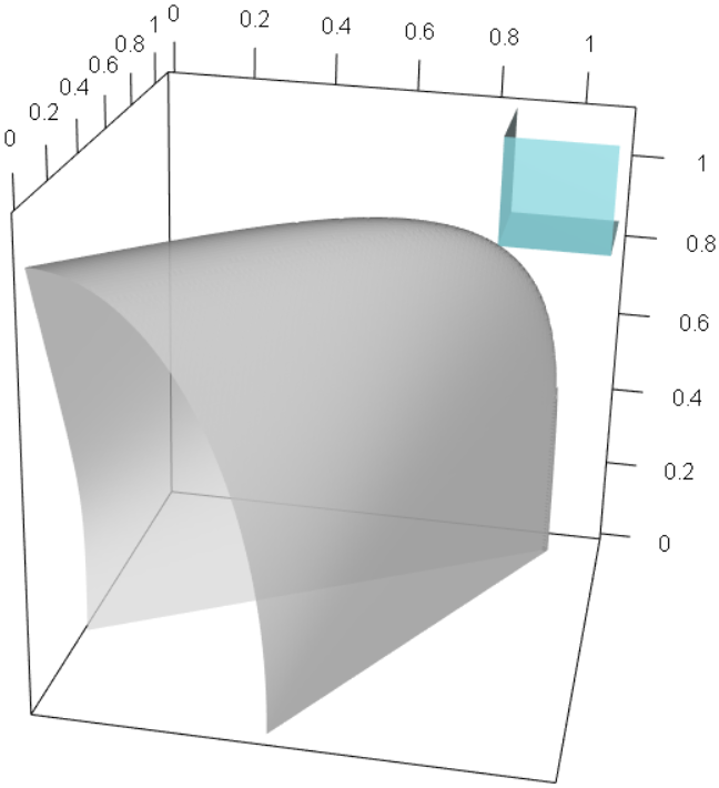
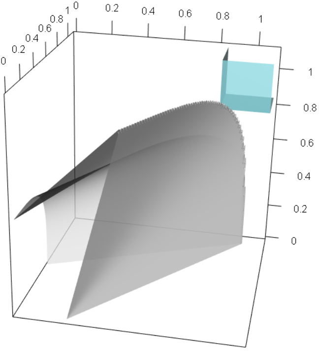
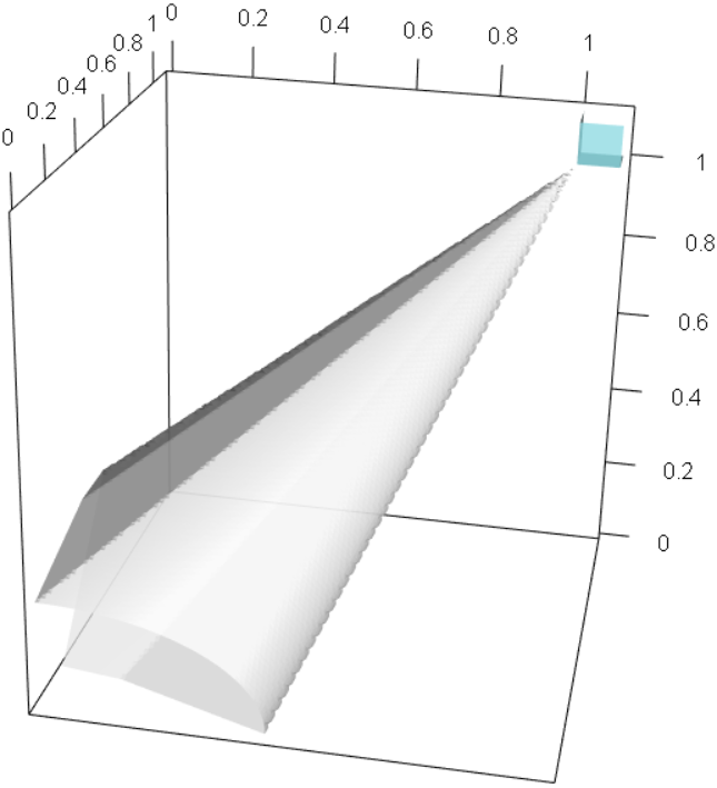
Fig. 4 demonstrates the sets G={𝒙∈ℝ3:g⁡(𝒙)=1}G=\{\bm{x}\in\mathbb{R}^{3}:g(\bm{x})=1\} for this gauge function, with α∈{0.25,0.5,0.75}\alpha\in\{0.25,0.5,0.75\}, β=0.25\beta=0.25 and γ=0.5\gamma=0.5. As was the case with the bivariate inverted logistic copula, the surface corresponding to the set GG is smooth and convex, and considering the intersection of GG with the lines xi=1x_{i}=1, i=1,2,3i=1,2,3, shows that each variable takes its largest values while the other two take their smallest.

Refer to caption
Figure 4: The set G={𝒙∈ℝ3:g⁡(𝒙)=1}G=\{\bm{x}\in\mathbb{R}^{3}:g(\bm{x})=1\} for a trivariate vine with three inverted logistic pair copula components (grey) and the boundary of the set [η{1,2,3},1)3[\eta_{\{1,2,3\}},1)^{3} (blue): α=0.25\alpha=0.25 (left), α=0.5\alpha=0.5 (centre), α=0.75\alpha=0.75 (right); β=0.25\beta=0.25 and γ=0.5\gamma=0.5.

From Section 4.1, we already know that the minimum in (5) occurs when x1=x3=1x_{1}=x_{3}=1, since g⁡(𝒙)g(\bm{x}) is increasing with respect to both these variables. In Section C of the Supplementary Material, we show that the gauge function is also increasing with respect to x2≥1x_{2}\geq 1. Hence, we know that the minimum occurs at 𝒙=𝟏\bm{x}=\bm{1}, i.e., that the intersection of GG and [η{1,2,3},∞)3[\eta_{\{1,2,3\}},\infty)^{3} occurs on the diagonal x1=x2=x3x_{1}=x_{2}=x_{3}. This is supported by the plots in Fig. 4, and yields

η{1,2,3}=g​(1,1,1)−1=[1+{(2α−1)1/γ+(2β−1)1/γ}γ]−1.\displaystyle\eta_{\{1,2,3\}}=g(1,1,1)^{-1}=\left[1+\left\{\left(2^{\alpha}-1\right)^{1/\gamma}+\left(2^{\beta}-1\right)^{1/\gamma}\right\}^{\gamma}\right]^{-1}. (22)

As min⁡(α,β,γ)→1\min\left(\alpha,\beta,\gamma\right)\rightarrow 1, η{1,2,3}→1/3\eta_{\{1,2,3\}}\rightarrow 1/3, corresponding to complete independence, and as max⁡(α,β,γ)→0\max\left(\alpha,\beta,\gamma\right)\rightarrow 0, η{1,2,3}→1\eta_{\{1,2,3\}}\rightarrow 1.

4.1.2 Calculation of η{1,3}\eta_{\{1,3\}}

We now consider the coefficient of tail dependence for the variables X1X_{1} and X3X_{3}, i.e., the pair that is not directly linked in tree T1T_{1} of the underlying vine. The joint density of X1X_{1} and X3X_{3} cannot be found analytically for a trivariate vine with inverted logistic pair copula components; we therefore use the method discussed in Section 2.2, with the gauge function for this pair of variables being g{1,3}​(x1,x3)=minx2≥0⁡g⁡(𝒙)g_{\{1,3\}}(x_{1},x_{3})=\min_{x_{2}\geq 0}g(\bm{x}), for g⁡(𝒙)g(\bm{x}) in (21). To demonstrate the boundary of the scaled sample cloud, we carry out this minimisation numerically. In the left panel of Fig. 5, we plot the set G{1,3}G_{\{1,3\}} for (α,β,γ)=(0.5,0.25,0.5)(\alpha,\beta,\gamma)=(0.5,0.25,0.5), chosen to match the parameter values for the central panel of Fig. 4.

Figure 5: Left: for (α,β,γ)=(0.5,0.25,0.5)(\alpha,\beta,\gamma)=(0.5,0.25,0.5), the sets G{1,3}G_{\{1,3\}} (grey) and [η{1,3},1)2[\eta_{\{1,3\}},1)^{2} (blue). Right: values of η{1,3}\eta_{\{1,3\}} for γ∈[0.05,0.95]\gamma\in[0.05,0.95] and (α,β)∈{(0.25,0.25)(\alpha,\beta)\in\{(0.25,0.25),(0.25,0.5)(0.25,0.5),(0.5,0.5)(0.5,0.5),(0.25,0.75)(0.25,0.75),(0.5,0.75)(0.5,0.75),(0.75,0.75)}(0.75,0.75)\} (top to bottom).

To calculate η{1,3}\eta_{\{1,3\}}, we follow the steps in Section 2.2, where we have η{1,3}={minx1,x3≥1⁡g{1,3}​(x1,x3)}−1={minx1,x3≥1,x2≥0⁡g⁡(x1,x2,x3)}−1\eta_{\{1,3\}}=\left\{\min_{x_{1},x_{3}\geq 1}g_{\{1,3\}}(x_{1},x_{3})\right\}^{-1}=\left\{\min_{x_{1},x_{3}\geq 1,x_{2}\geq 0}g(x_{1},x_{2},x_{3})\right\}^{-1}. We have already seen that g⁡(𝒙)g(\bm{x}) is increasing with respect to x1x_{1} and x3x_{3}, so we focus on x1=x3=1x_{1}=x_{3}=1, and have η{1,3}={minv≥0⁡g⁡(1,v,1)}−1\eta_{\{1,3\}}=\left\{\min_{v\geq 0}g(1,v,1)\right\}^{-1}. That is,

η{1,3}=(v+[{(1+v1/α)α−v}1/γ+{(1+v1/β)β−v}1/γ]γ)−1,\eta_{\{1,3\}}=\left(v+\left[\left\{\left(1+v^{1/\alpha}\right)^{\alpha}-v\right\}^{1/\gamma}+\left\{\left(1+v^{1/\beta}\right)^{\beta}-v\right\}^{1/\gamma}\right]^{\gamma}\right)^{-1},

with vv satisfying d​g​(1,v,1)/d​v=0dg(1,v,1)/dv=0, i.e.,

1+[{(1+v1/α)α−v}1/γ+{(1+v1/β)β−v}1/γ]γ−1⋅[{(1+v−1/α)α−1−1}{(1+v1/α)α−v}−1+1/γ\displaystyle 1+\left[\left\{\left(1+v^{1/\alpha}\right)^{\alpha}-v\right\}^{1/\gamma}+\left\{\left(1+v^{1/\beta}\right)^{\beta}-v\right\}^{1/\gamma}\right]^{\gamma-1}\cdot\bigg[\left\{(1+v^{-1/\alpha})^{\alpha-1}-1\right\}\left\{(1+v^{1/\alpha})^{\alpha}-v\right\}^{-1+1/\gamma}
+{(1+v−1/β)β−1−1}{(1+v1/β)β−v}−1+1/γ]=0.\displaystyle\hskip 85.35826pt+\left\{(1+v^{-1/\beta})^{\beta-1}-1\right\}\left\{(1+v^{1/\beta})^{\beta}-v\right\}^{-1+1/\gamma}\bigg]=0. (23)

In Section C of the Supplementary Material, we show that (23) has a unique solution that lies in the range (0,1)(0,1). In general, equation (23) has no closed form solution, except in the case where α=β\alpha=\beta, which leads to

v={(1−2−γ)−1/(1−α)−1}−α;η{1,3}={(1−2−γ)−1/(1−α)−1}α1−2γ+2γ(1−2−γ)−α/(1−α),v=\left\{(1-2^{-\gamma})^{-1/(1-\alpha)}-1\right\}^{-\alpha}~~;~~\eta_{\{1,3\}}=\frac{\left\{\left(1-2^{-\gamma}\right)^{-1/(1-\alpha)}-1\right\}^{\alpha}}{1-2^{\gamma}+2^{\gamma}\left(1-2^{-\gamma}\right)^{-\alpha/(1-\alpha)}},

but it can be solved numerically when α≠β\alpha\neq\beta. In the right panel of Fig. 5, we demonstrate the resulting value of η{1,3}\eta_{\{1,3\}} for a variety of α,β\alpha,\beta and γ\gamma values. We note that η{1,3}∈(0.5,1)\eta_{\{1,3\}}\in(0.5,1), revealing flexibility in the asymptotic independence features this model can capture. In particular, for the α=β\alpha=\beta case, η{1,3}=1−γ​ln⁡2+o⁡(γ)↗1\eta_{\{1,3\}}=1-\gamma\ln 2+o(\gamma)\nearrow 1, as γ↘0\gamma\searrow 0.

4.2 Higher dimensional results

We now extend the results of Section 4.1 by considering vine copulas with dimension d>3d>3 constructed from inverted extreme value pair copulas, with the aim being to find the gauge function and value of η𝒟\eta_{\mathcal{D}} in each case. We focus on copulas with two types of underlying structure: the class of vine copulas known as DD-vines, where all trees in the vine are paths; and CC-vines, which have exactly one node that is connected to all other nodes in each tree. These correspond to the two classes demonstrated in Fig. 3 for the case d=4d=4. In the final part of this section, we demonstrate the values of η𝒟\eta_{\mathcal{D}} calculated using these gauge functions for both classes of model.

4.2.1 Gauge functions for DD-vines

A dd-dimensional DD-vine is made up of (d−1)(d-1) trees, labelled T1,…,Td−1T_{1},\ldots,T_{d-1}, and a total of (d−1)​d/2(d-1)d/2 edges. We suppose that the pair copula represented by each edge is an inverted extreme value copula, with the superscript on the exponent measure corresponding to the edge-label, as in the trivariate case. For the four-dimensional example in Fig. 3, we have

−\displaystyle- ln⁡f⁡(t​𝒙)=−ln⁡f1​(t​x1)−ln⁡f2​(t​x2)−ln⁡f3​(t​x3)−ln⁡f4​(t​x4)\displaystyle\ln f(t\bm{x})=-\ln f_{1}(tx_{1})-\ln f_{2}(tx_{2})-\ln f_{3}(tx_{3})-\ln f_{4}(tx_{4})
−ln⁡c12​{F1​(t​x1),F2​(t​x2)}−ln⁡c23​{F2​(t​x2),F3​(t​x3)}−ln⁡c34​{F3​(t​x3),F4​(t​x4)}\displaystyle~~-\ln c_{12}\left\{F_{1}(tx_{1}),F_{2}(tx_{2})\right\}-\ln c_{23}\left\{F_{2}(tx_{2}),F_{3}(tx_{3})\right\}-\ln c_{34}\left\{F_{3}(tx_{3}),F_{4}(tx_{4})\right\}
−ln⁡c13|2​{F1|2​(t​x1|t​x2),F3|2​(t​x3|t​x2)}−ln⁡c24|3​{F2|3​(t​x2|t​x3),F4|3​(t​x4|t​x3)}\displaystyle~~-\ln c_{13|2}\left\{F_{1|2}(tx_{1}|tx_{2}),F_{3|2}(tx_{3}|tx_{2})\right\}-\ln c_{24|3}\left\{F_{2|3}(tx_{2}|tx_{3}),F_{4|3}(tx_{4}|tx_{3})\right\}
−ln⁡c14|23​{F1|23​(t​x1|t​x2,t​x3),F4|23​(t​x4|t​x2,t​x3)}.\displaystyle~~-\ln c_{14|23}\left\{F_{1|23}(tx_{1}|tx_{2},tx_{3}),F_{4|23}(tx_{4}|tx_{2},tx_{3})\right\}. (24)

We note that several of these terms can be thought of in terms of lower-dimensional vine copulas that are subsets of the four-dimensional vine. In particular, all terms in the trivariate formula (19) for the set of variables (X1,X2,X3)(X_{1},X_{2},X_{3}) appear in (24). Let f123f_{123} denote the joint density corresponding to this trivariate case. The density f234f_{234} corresponding to variables (X2,X3,X4)(X_{2},X_{3},X_{4}) also comes from a trivariate vine copula equivalent to f123f_{123} up to a labelling of the variables. The sections of the four-dimensional vine corresponding to these two trivariate subsets are highlighted in Fig. 6, and can be thought of as sub-vines of the overall vine copula. We note that these two sub-vines overlap in the centre, as they share the variables (X2,X3)(X_{2},X_{3}). This suggests that if we try to represent −ln⁡f-\ln f for the overall model in terms of −ln⁡f123-\ln f_{123} and −ln⁡f234-\ln f_{234}, we will count the section corresponding to −ln⁡f23-\ln f_{23} twice, with f23f_{23} denoting the joint density of (X2,X3)(X_{2},X_{3}). Taking this inclusion-exclusion into account, equation (24) can be simplified to

−ln⁡f⁡(t​𝒙)=\displaystyle-\ln f(t\bm{x})= −ln⁡f123​(t​x1,t​x2,t​x3)−ln⁡f234​(t​x2,t​x3,t​x4)+ln⁡f23​(t​x2,t​x3)\displaystyle-\ln f_{123}(tx_{1},tx_{2},tx_{3})-\ln f_{234}(tx_{2},tx_{3},tx_{4})+\ln f_{23}(tx_{2},tx_{3})
−ln⁡c14|23​{F1|23​(t​x1|t​x2,t​x3),F4|23​(t​x4|t​x2,t​x3)}.\displaystyle-\ln c_{14|23}\left\{F_{1|23}(tx_{1}|tx_{2},tx_{3}),F_{4|23}(tx_{4}|tx_{2},tx_{3})\right\}. (25)
Refer to caption
Figure 6: Trivariate subsets of the four-dimensional DD-vine.

In Section D of the Supplementary Material, we show that the gauge function can be written in terms of the gauge functions of the three sub-vines highlighted in Fig. 6 and the exponent measure corresponding to the pair copula in tree T3T_{3}. In particular,

g⁡(𝒙)\displaystyle g(\bm{x}) =g{2,3}​(x2,x3)+V{14|23}​{1g{1,2,3}​(x1,x2,x3)−g{2,3}​(x2,x3),1g{2,3,4}​(x2,x3,x4)−g{2,3}​(x2,x3)},\displaystyle=g_{\{2,3\}}(x_{2},x_{3})+V^{\{14|23\}}\left\{\frac{1}{g_{\{1,2,3\}}(x_{1},x_{2},x_{3})-g_{\{2,3\}}(x_{2},x_{3})},\frac{1}{g_{\{2,3,4\}}(x_{2},x_{3},x_{4})-g_{\{2,3\}}(x_{2},x_{3})}\right\}, (26)

for x1,x2,x3≥0x_{1},x_{2},x_{3}\geq 0. For DD-vine copulas, this same structure can be extended to higher dimensions, creating an iterative formula for calculating the gauge function; this is stated in Theorem 1.

Theorem 1.

The gauge function for a dd-dimensional DD-vine with inverted extreme value pair copula components is given by

g\displaystyle g (𝒙)=g𝒟\{1,d}(𝒙−{1,d})+V{1,d∣𝒟\{1,d}}{1g𝒟\{d}​(𝒙−{d})−g𝒟\{1,d}​(𝒙−{1,d}),1g𝒟\{1}​(𝒙−{1})−g𝒟\{1,d}​(𝒙−{1,d})},\displaystyle(\bm{x})=g_{\mathcal{D}\backslash\{1,d\}}(\bm{x}_{-\{1,d\}})+V^{\{1,d\mid\mathcal{D}\backslash\{1,d\}\}}\left\{\frac{1}{g_{\mathcal{D}\backslash\{d\}}(\bm{x}_{-\{d\}})-g_{\mathcal{D}\backslash\{1,d\}}(\bm{x}_{-\{1,d\}})},\frac{1}{g_{\mathcal{D}\backslash\{1\}}(\bm{x}_{-\{1\}})-g_{\mathcal{D}\backslash\{1,d\}}(\bm{x}_{-\{1,d\}})}\right\},

for xi≥0x_{i}\geq 0, i=1,…,di=1,\ldots,d.

Theorem 1 is proved in the Appendix. We discuss how to obtain η𝒟\eta_{\mathcal{D}} in Section 4.2.3.

4.2.2 Gauge functions for CC-vines

Using similar arguments as for the DD-vines in Section 4.2.1, we can construct an iterative formula for the gauge functions of dd-dimensional CC-vines. We now consider the sub-vines as corresponding to the sets of variables 𝑿−d\bm{X}_{-d} and 𝑿−(d−1)\bm{X}_{-(d-1)}, which overlap at 𝑿−{(d−1),d}\bm{X}_{-\{(d-1),d\}}. This is demonstrated in Fig. 7 for the four-dimensional case. Following the same steps as in the previous section, we obtain the gauge function

g⁡(𝒙)=\displaystyle g(\bm{x})= g𝒟\{(d−1,d}(𝒙−{d−1,d})\displaystyle g_{\mathcal{D}\backslash\{(d-1,d\}}(\bm{x}_{-\{d-1,d\}})
+V{d−1,d∣𝒟\{d−1,d}}{1g𝒟\{d}​(𝒙−{d})−g𝒟\{d−1,d}​(𝒙−{d−1,d}),1g𝒟\{d−1}​(𝒙−{d−1})−g𝒟\{d−1,d}​(𝒙−{d−1,d})},\displaystyle+V^{\{d-1,d\mid\mathcal{D}\backslash\{d-1,d\}\}}\bigg\{\frac{1}{g_{\mathcal{D}\backslash\{d\}}(\bm{x}_{-\{d\}})-g_{\mathcal{D}\backslash\{d-1,d\}}(\bm{x}_{-\{d-1,d\}})},\frac{1}{g_{\mathcal{D}\backslash\{d-1\}}(\bm{x}_{-\{d-1\}})-g_{\mathcal{D}\backslash\{d-1,d\}}(\bm{x}_{-\{d-1,d\}})}\bigg\},

with xi≥0x_{i}\geq 0, i=1,…,di=1,\ldots,d.

Refer to caption
Figure 7: Trivariate subsets of the four-dimensional CC-vine.

4.2.3 Calculating η𝒟\eta_{\mathcal{D}} for dd-dimensional DD-vines and CC-vines with inverted logistic components

As for the trivariate vine copula examples with inverted logistic pair copula components, numerical results suggest that the intersection of the set G={𝒙∈ℝd:g⁡(𝒙)=1}G=\{\bm{x}\in\mathbb{R}^{d}:g(\bm{x})=1\} and [η𝒟,∞)d[\eta_{\mathcal{D}},\infty)^{d} for these DD-vines and CC-vines occurs when x1=…=xdx_{1}=\ldots=x_{d}. As before, this suggests that η𝒟=g​(1,…,1)−1\eta_{\mathcal{D}}=g(1,\ldots,1)^{-1} in this case.

Figure 8: Values of η𝒟\eta_{\mathcal{D}} for d∈{2,…,d}d\in\{2,\ldots,d\} for a dd-dimensional DD-vine or CC-vine constructed from inverted logistic pair copulas all having equal dependence parameter α∈{0.1,…,0.9}\alpha\in\{0.1,\ldots,0.9\}.

Due to the nested structure of the gauge functions, the value of η𝒟\eta_{\mathcal{D}} can be written in terms of the values of η𝒞\eta_{\mathcal{C}} for various sub-vines of the copula, and the exponent measure corresponding to tree Td−1T_{d-1} of the vine. In particular, for DD-vines, we have

η𝒟={η𝒟\{1,d}−1+V{1,d|𝒟\{1,d}}(1η𝒟\{d}−1−η𝒟\{1,d}−1,1η𝒟\{1}−1−η𝒟\{1,d}−1)}−1\displaystyle\eta_{\mathcal{D}}=\left\{\eta_{\mathcal{D}\backslash\{1,d\}}^{-1}+V^{\{1,d|\mathcal{D}\backslash\{1,d\}\}}\left(\frac{1}{\eta_{\mathcal{D}\backslash\{d\}}^{-1}-\eta_{\mathcal{D}\backslash\{1,d\}}^{-1}},\frac{1}{\eta_{\mathcal{D}\backslash\{1\}}^{-1}-\eta_{\mathcal{D}\backslash\{1,d\}}^{-1}}\right)\right\}^{-1} (27)

and for CC-vines,

η𝒟={η𝒟\{d−1,d}−1+V{d−1,d|𝒟\{d−1,d}}(1η𝒟\{d}−1−η𝒟\{d−1,d}−1,1η𝒟\{(d−1)}−1−η𝒟\{d−1,d}−1)}−1.\eta_{\mathcal{D}}=\left\{\eta_{\mathcal{D}\backslash\{d-1,d\}}^{-1}+V^{\{d-1,d|\mathcal{D}\backslash\{d-1,d\}\}}\left(\frac{1}{\eta_{\mathcal{D}\backslash\{d\}}^{-1}-\eta_{\mathcal{D}\backslash\{d-1,d\}}^{-1}},\frac{1}{\eta_{\mathcal{D}\backslash\{(d-1)\}}^{-1}-\eta_{\mathcal{D}\backslash\{d-1,d\}}^{-1}}\right)\right\}^{-1}.

Setting η𝒞=1\eta_{\mathcal{C}}=1 for |𝒞|=1|\mathcal{C}|=1, we now have an iterative method for calculating the values of η𝒟\eta_{\mathcal{D}} for these classes of model for d≥3d\geq 3 dimensions.

As an example, we consider the case where all the pair copulas of the vine are inverted logistic with the same dependence parameter α∈(0,1)\alpha\in(0,1). In this case, the known value of η{1,2}\eta_{\{1,2\}} for the bivariate copula is 2−α2^{-\alpha}. We can therefore use our iterative formulas to calculate η𝒟\eta_{\mathcal{D}} for higher dimensional vine copulas. Since the exponent is homogeneous of order −1-1, the expression for η𝒟\eta_{\mathcal{D}} in (27) in this case simplifies to

η𝒟={η𝒟\{1,d}−1+2α​(η𝒟\{d}−1−η𝒟\{1,d}−1)}−1,\displaystyle\eta_{\mathcal{D}}=\left\{\eta^{-1}_{\mathcal{D}\backslash\{1,d\}}+2^{\alpha}\left(\eta^{-1}_{\mathcal{D}\backslash\{d\}}-\eta^{-1}_{\mathcal{D}\backslash\{1,d\}}\right)\right\}^{-1}, (28)

and we can use the iterative method to derive the exact value of η𝒟\eta_{\mathcal{D}} for any dd-dimensional DD-vine copula. For this example, we can extend the results to higher dd-dimensional vine copulas, yielding, for d≥3d\geq 3,

η𝒟\displaystyle\eta_{\mathcal{D}} ={{1+2α​∑k=1(d−1)/2(2α−1)2​(k−1)+1}−1,for d odd,{2α​∑k=1d/2(2α−1)2​(k−1)}−1,for d even,={[1+2α−12−2α​{1−(2α−1)d−1}]−1,for d odd,[12−2α​{1−(2α−1)d}]−1,for d even,\displaystyle=\begin{cases}\left\{1+2^{\alpha}\sum_{k=1}^{(d-1)/2}\left(2^{\alpha}-1\right)^{2(k-1)+1}\right\}^{-1},&\text{for $d$ odd},\\ \left\{2^{\alpha}\sum_{k=1}^{d/2}\left(2^{\alpha}-1\right)^{2(k-1)}\right\}^{-1},&\text{for $d$ even,}\end{cases}~=~\begin{cases}\left[1+\frac{2^{\alpha}-1}{2-2^{\alpha}}\left\{1-(2^{\alpha}-1)^{d-1}\right\}\right]^{-1},&\text{for $d$ odd},\\ \left[\frac{1}{2-2^{\alpha}}\left\{1-(2^{\alpha}-1)^{d}\right\}\right]^{-1},&\text{for $d$ even},\end{cases} (29)

which can be shown to be decreasing in dd. We prove result (29) by induction in Section F of the Supplementary Material. We note that when the pair copulas, and therefore the corresponding exponent measures, are all taken to be identical, the value of η𝒟\eta_{\mathcal{D}} is the same for the DD-vines and CC-vines of the same dimension. These values are demonstrated in Fig. 8 for α∈{0.1,…,0.9}\alpha\in\{0.1,\ldots,0.9\} and d∈{2,…,10}d\in\{2,\ldots,10\}, where we have η𝒟<1\eta_{\mathcal{D}}<1 in all cases, corresponding to asymptotic independence. Complete independence in the dd-dimensional vine copula corresponds to η𝒟=1/d\eta_{\mathcal{D}}=1/d. We see from Fig. 8 that for α=0.9\alpha=0.9, we approach this case, while for α=0.1\alpha=0.1, the values of η𝒟\eta_{\mathcal{D}} are close to 1, corresponding to strong residual dependence. These models are therefore able to capture a range of sub-asymptotic dependence strengths in the asymptotic independence case.

5 Trivariate vine copulas with inverted extreme value and extreme value copula components

5.1 Overview

We have so far focused on the tail dependence properties of vine copulas with inverted extreme value pair copula components. Now, we investigate these same properties for trivariate vine copulas where the components are either extreme value or inverted extreme value copulas. We consider five such cases, which along with the results in Section 4.1 cover the range of possible scenarios. In Section 5.2.1, the two copulas in tree T1T_{1} of Fig. 2 belong to the inverted extreme value class, and there is an extreme value copula in tree T2T_{2}; tree T1T_{1} has one extreme value and one inverted extreme value copula in Sections 5.2.2 and 5.2.3, with the copula in tree T2T_{2} being either inverted extreme value or extreme value, respectively; and in Sections 5.2.4 and 5.2.5, both copulas in tree T1T_{1} are from the extreme value family with the copula in tree T2T_{2} being inverted extreme value and extreme value in the respective sections. This section will therefore consist of a series of examples, and the gauge functions resulting from these vine structures generally have a complicated form, with the corresponding sets GG exhibiting interesting shapes including non-convexity and non-smoothness. This differs from other well-known examples such as the multivariate Gaussian distribution. The gauge function calculations are provided in Sections G to I of the Supplementary Material for each of these cases, with the extreme value components satisfying conditions analogous to (12). Specifically, let h{12}​(w)h^{\{12\}}(w), h{23}​(w)h^{\{23\}}(w), h{13|2}​(w)h^{\{13|2\}}(w) denote the spectral density for each pair copula component. We assume that each of these densities has h{⋅}​(w)∼c1{⋅}​(1−w)s1{⋅}h^{\{\cdot\}}(w)\sim c_{1}^{\{\cdot\}}(1-w)^{s_{1}^{\{\cdot\}}} as w↗1w\nearrow 1 and h{⋅}​(w)∼c2{⋅}​ws2{⋅}h^{\{\cdot\}}(w)\sim c_{2}^{\{\cdot\}}w^{s_{2}^{\{\cdot\}}} as w↘0w\searrow 0, for some c1{⋅},c2{⋅}∈ℝc_{1}^{\{\cdot\}},c_{2}^{\{\cdot\}}\in\mathbb{R} and s1{⋅},s2{⋅}>−1s_{1}^{\{\cdot\}},s_{2}^{\{\cdot\}}>-1.

Our results are summarised in Section 5.2, where we also investigate the corresponding values of η{1,2,3}\eta_{\{1,2,3\}} and η{1,3}\eta_{\{1,3\}} for logistic and inverted logistic examples, with exponent measure (10). In some subsections, this is achieved by obtaining results for more general gauge functions. In other cases this is not possible, and we focus only on the (inverted) logistic examples, but suggest that similar strategies could be used for other cases. Whether the copula is logistic or inverted logistic, we denote the parameters associated with exponent measures of copulas c12c_{12}, c23c_{23} and c13|2c_{13|2} by α,β,γ∈(0,1)\alpha,\beta,\gamma\in(0,1), respectively. We note that in the logistic case, we have s1{12}=s2{12}=1/α−2s^{\{12\}}_{1}=s^{\{12\}}_{2}=1/\alpha-2; s1{23}=s2{23}=1/β−2s^{\{23\}}_{1}=s^{\{23\}}_{2}=1/\beta-2 and s1{13|2}=s2{13|2}=1/γ−2s^{\{13|2\}}_{1}=s^{\{13|2\}}_{2}=1/\gamma-2.

5.2 Gauge functions for trivariate vines with extreme value and inverted extreme value components

5.2.1 Inverted extreme value copulas in T1T_{1}; extreme value copula in T2T_{2}

The calculations in the Supplementary Material demonstrate that the gauge function is

g⁡(𝒙)=\displaystyle g(\bm{x})= (2+sm{13∣2})​max​{V{12}​(x1−1,x2−1),V{23}​(x2−1,x3−1)}−(1+sm{13∣2})​min​{V{12}​(x1−1,x2−1),V{23}​(x2−1,x3−1)},\displaystyle\left(2+s_{\text{m}}^{\{13\mid 2\}}\right)\max\left\{V^{\{12\}}\left(x_{1}^{-1},x_{2}^{-1}\right),V^{\{23\}}\left(x_{2}^{-1},x_{3}^{-1}\right)\right\}-\left(1+s_{\text{m}}^{\{13\mid 2\}}\right)\min\left\{V^{\{12\}}\left(x_{1}^{-1},x_{2}^{-1}\right),V^{\{23\}}\left(x_{2}^{-1},x_{3}^{-1}\right)\right\},

with min⁡(x1,x2,x3)≥0\min(x_{1},x_{2},x_{3})\geq 0, and

s{13∣2}m=s{13∣2}1𝟙{V{12}(x1−1,x2−1)≥V{23}(x2−1,x3−1)}+s{13∣2}2𝟙{V{12}(x1−1,x2−1)<V{23}(x2−1,x3−1)}>−1.s^{\{13\mid 2\}}_{\text{m}}=s^{\{13\mid 2\}}_{1}\mathbbm{1}_{\left\{V^{\{12\}}\left(x_{1}^{-1},~x_{2}^{-1}\right)\geq V^{\{23\}}\left(x_{2}^{-1},~x_{3}^{-1}\right)\right\}}+s^{\{13\mid 2\}}_{2}\mathbbm{1}_{\left\{V^{\{12\}}\left(x_{1}^{-1},~x_{2}^{-1}\right)<V^{\{23\}}\left(x_{2}^{-1},~x_{3}^{-1}\right)\right\}}~{{\color[rgb]{0,0,0}>-1}}.

To calculate η{1,2,3}\eta_{\{1,2,3\}}, we must here consider two separate cases. First, we assume that V{12}​(x1−1,x2−1)≥V{23}​(x2−1,x3−1)V^{\{12\}}\left(x_{1}^{-1},x_{2}^{-1}\right)\geq V^{\{23\}}\left(x_{2}^{-1},x_{3}^{-1}\right), so the gauge function simplifies to

g⁡(𝒙)=(2+sm{13∣2})​V{12}​(x1−1,x2−1)−(1+sm{13∣2})​V{23}​(x2−1,x3−1).g(\bm{x})=\left(2+s_{\text{m}}^{\{13\mid 2\}}\right)V^{\{12\}}\left(x_{1}^{-1},x_{2}^{-1}\right)-\left(1+s_{\text{m}}^{\{13\mid 2\}}\right)V^{\{23\}}\left(x_{2}^{-1},x_{3}^{-1}\right).

Since sm{13∣2}>−1s^{\{13\mid 2\}}_{\text{m}}>-1, g⁡(𝒙)g(\bm{x}) is non-decreasing in x1x_{1} and we can set x1=1x_{1}=1 to find the solution of (5). We therefore need to minimise

g⁡(1,x2,x3)=(2+sm{13∣2})​V{12}​(1,x2−1)−(1+sm{13∣2})​V{23}​(x2−1,x3−1),g(1,x_{2},x_{3})=\left(2+s_{\text{m}}^{\{13\mid 2\}}\right)V^{\{12\}}\left(1,x_{2}^{-1}\right)-\left(1+s_{\text{m}}^{\{13\mid 2\}}\right)V^{\{23\}}\left(x_{2}^{-1},x_{3}^{-1}\right),

such that V{12}​(1,x2−1)≥V{23}​(x2−1,x3−1)V^{\{12\}}\left(1,x_{2}^{-1}\right)\geq V^{\{23\}}\left(x_{2}^{-1},x_{3}^{-1}\right). Now, the function g⁡(1,x2,x3)g(1,x_{2},x_{3}) is non-increasing in x3x_{3}, which should therefore be taken to be as large as possible. Since V{23}​(x2−1,x3−1)V^{\{23\}}\left(x_{2}^{-1},x_{3}^{-1}\right) is non-decreasing in x3x_{3}, this function should also be as large as possible, i.e., the largest value of x3x_{3} occurs when V{23}​(x2−1,x3−1)=V{12}​(1,x2−1)V^{\{23\}}\left(x_{2}^{-1},x_{3}^{-1}\right)=V^{\{12\}}\left(1,x_{2}^{-1}\right), and the gauge function becomes

g⁡(1,x2,x3)=(2+sm{13∣2})​V{12}​(1,x2−1)−(1+sm{13∣2})​V{12}​(1,x2−1)=V{12}​(1,x2−1).g(1,x_{2},x_{3})=\left(2+s_{\text{m}}^{\{13\mid 2\}}\right)V^{\{12\}}\left(1,x_{2}^{-1}\right)-\left(1+s_{\text{m}}^{\{13\mid 2\}}\right)V^{\{12\}}\left(1,x_{2}^{-1}\right)=V^{\{12\}}\left(1,x_{2}^{-1}\right).

Again, this is non-decreasing in x2x_{2}, so the minimum occurs when x2=1x_{2}=1, i.e., min𝒙:min⁡(𝒙)=1g(𝒙)=V{12}(1,1)\min_{\bm{x}:\min(\bm{x})=1}g(\bm{x})=V^{\{12\}}\left(1,1\right). For the case where V{12}​(x1−1,x2−1)≤V{23}​(x2−1,x3−1)V^{\{12\}}\left(x_{1}^{-1},x_{2}^{-1}\right)\leq V^{\{23\}}\left(x_{2}^{-1},x_{3}^{-1}\right), by a similar argument, min𝒙:min⁡(𝒙)=1g(𝒙)=V{23}(1,1)\min_{\bm{x}:\min(\bm{x})=1}g(\bm{x})=V^{\{23\}}\left(1,1\right). In summary, we have

η{1,2,3}={min𝒙:min⁡(𝒙)=1g(𝒙)}−1=[max{V{12}(1,1),V{23}(1,1)}]−1=min[{V{12}(1,1)}−1,{V{23}(1,1)}−1].\eta_{\{1,2,3\}}=\left\{\min\limits_{\bm{x}:\min(\bm{x})=1}g(\bm{x})\right\}^{-1}=\left[\max\left\{V^{\{12\}}\left(1,1\right),V^{\{23\}}\left(1,1\right)\right\}\right]^{-1}=\min\left[\left\{V^{\{12\}}\left(1,1\right)\right\}^{-1},\left\{V^{\{23\}}\left(1,1\right)\right\}^{-1}\right].

For the value of η{1,3}\eta_{\{1,3\}}, we observe that

g⁡(1,0,1)\displaystyle g(1,0,1) =(2+sm{13∣2})​max​{V{12}​(1,∞),V{23}​(∞,1)}−(1+sm{13∣2})​min​{V{12}​(1,∞),V{23}​(∞,1)}\displaystyle=\left(2+s_{\text{m}}^{\{13\mid 2\}}\right)\max\left\{V^{\{12\}}\left(1,\infty\right),V^{\{23\}}\left(\infty,1\right)\right\}-\left(1+s_{\text{m}}^{\{13\mid 2\}}\right)\min\left\{V^{\{12\}}\left(1,\infty\right),V^{\{23\}}\left(\infty,1\right)\right\}
=(2+sm{13∣2})−(1+sm{13∣2})=1.\displaystyle=\left(2+s_{\text{m}}^{\{13\mid 2\}}\right)-\left(1+s_{\text{m}}^{\{13\mid 2\}}\right)=1.

As discussed in Section 2.2, this is the smallest possible value of minx1,x3≥1,x2≥0⁡g⁡(𝒙)\min_{x_{1},x_{3}\geq 1,x_{2}\geq 0}g(\bm{x}), and therefore must be our required minimum. We therefore have η{1,3}=1\eta_{\{1,3\}}=1.

For an example with logistic and inverted logistic components, the gauge function is

g⁡(𝒙)=\displaystyle g(\bm{x})= (1/γ)​max​{(x11/α+x21/α)α,(x21/β+x31/β)β}−(1/γ−1)​min​{(x11/α+x21/α)α,(x21/β+x31/β)β},\displaystyle\left(1/\gamma\right)\max\left\{\left(x_{1}^{1/\alpha}+x_{2}^{1/\alpha}\right)^{\alpha},\left(x_{2}^{1/\beta}+x_{3}^{1/\beta}\right)^{\beta}\right\}-\left(1/\gamma-1\right)\min\left\{\left(x_{1}^{1/\alpha}+x_{2}^{1/\alpha}\right)^{\alpha},\left(x_{2}^{1/\beta}+x_{3}^{1/\beta}\right)^{\beta}\right\},

with η{1,2,3}=min⁡(1/2α,1/2β)\eta_{\{1,2,3\}}=\min\left(1/2^{\alpha},1/2^{\beta}\right) and η{1,3}=1\eta_{\{1,3\}}=1.

In Fig. 9, we demonstrate the set G={𝒙∈ℝ3:g⁡(𝒙)=1}G=\{\bm{x}\in\mathbb{R}^{3}:g(\bm{x})=1\} for this example, with α∈{0.25,0.5,0.75}\alpha\in\{0.25,0.5,0.75\}, β=0.25\beta=0.25 and γ=0.5\gamma=0.5, where the surface corresponding to the set GG turns out to be non-convex. The plots in Fig. 9 support our analytical calculations. The intersection of GG and [η{1,2,3},1)3[\eta_{\{1,2,3\}},1)^{3} occurs at x1=x2=x3x_{1}=x_{2}=x_{3} in the first panel with α=β=0.25\alpha=\beta=0.25, and x3≥x1=x2x_{3}\geq x_{1}=x_{2} in the remaining two panels, where α>β\alpha>\beta. The gauge function for the pair of variables (X1,X3)(X_{1},X_{3}) is demonstrated in Fig. 10. This plot supports that η{1,3}=1\eta_{\{1,3\}}=1, and we note the non-convex shape of G{1,3}G_{\{1,3\}}.

Refer to caption
Figure 9: The set G={𝒙∈ℝ3:g⁡(𝒙)=1}G=\{\bm{x}\in\mathbb{R}^{3}:g(\bm{x})=1\} for a trivariate vine with inverted logistic copulas in T1T_{1} and a logistic copula in T2T_{2} (grey) and the boundary of the set [η{1,2,3},1)3[\eta_{\{1,2,3\}},1)^{3} (blue): α=0.25\alpha=0.25 (left), α=0.5\alpha=0.5 (centre), α=0.75\alpha=0.75 (right); β=0.25\beta=0.25 and γ=0.5\gamma=0.5.
Figure 10: The sets G{1,3}G_{\{1,3\}} (grey) and [η{1,3},1)2[\eta_{\{1,3\}},1)^{2} (blue) for (α,β,γ)=(0.5,0.25,0.5)(\alpha,\beta,\gamma)=(0.5,0.25,0.5).

5.2.2 Extreme value and inverted extreme value copulas in T1T_{1}; inverted extreme value copula in T2T_{2}

From the calculations in the Supplementary Material, the gauge function for this model is

g⁡(𝒙)={(2+s1{13∣2})​(1+s2{12})​(x2−x1)+V{23}​(x2−1,x3−1),0≤x1≤x2,x2+V{13∣2}​[{(x1−x2)​(2+s1{12})}−1,{V{23}​(x2−1,x3−1)−x2}−1],0≤x2<x1.\displaystyle g(\bm{x})=\begin{cases}\left(2+s_{1}^{\{13\mid 2\}}\right)\left(1+s_{2}^{\{12\}}\right)\left(x_{2}-x_{1}\right)+V^{\{23\}}\left(x_{2}^{-1},x_{3}^{-1}\right),&0\leq x_{1}\leq x_{2},\\ x_{2}+V^{\{13\mid 2\}}\left[\left\{\left(x_{1}-x_{2}\right)\left(2+s_{1}^{\{12\}}\right)\right\}^{-1},\left\{V^{\{23\}}\left(x_{2}^{-1},x_{3}^{-1}\right)-x_{2}\right\}^{-1}\right],&0\leq x_{2}<x_{1}.\end{cases}

To find η{1,2,3}\eta_{\{1,2,3\}}, there are two cases to consider. If x1≤x2x_{1}\leq x_{2}, it is clear that the function g⁡(𝒙)g(\bm{x}) is decreasing in x1x_{1}, which should therefore be taken to be as large as possible by fixing x1=x2x_{1}=x_{2}. The gauge function then simplifies to

g⁡(x2,x2,x3)=V{23}​(x2−1,x3−1),g(x_{2},x_{2},x_{3})=V^{\{23\}}\left(x_{2}^{-1},x_{3}^{-1}\right),

which is non-decreasing in both x2x_{2} and x3x_{3}, so we find the minimum by setting x2=x3=1x_{2}=x_{3}=1, yielding V{23}​(1,1)V^{\{23\}}(1,1). Similarly, for x2≤x1x_{2}\leq x_{1}, the gauge function is non-decreasing in x1x_{1}, and we can again fix x1=x2x_{1}=x_{2} with the resulting gauge function being

g⁡(x2,x2,x3)=x2+V{13∣2}​[0−1,{V{23}​(x2−1,x3−1)−x2}−1]=V{23}​(x2−1,x3−1).g(x_{2},x_{2},x_{3})=x_{2}+V^{\{13\mid 2\}}\left[0^{-1},\left\{V^{\{23\}}\left(x_{2}^{-1},x_{3}^{-1}\right)-x_{2}\right\}^{-1}\right]=V^{\{23\}}\left(x_{2}^{-1},x_{3}^{-1}\right).

Again, this is non-decreasing in x2x_{2} and x3x_{3}, so the minimum is given by V{23}​(1,1)V^{\{23\}}\left(1,1\right). Hence,

η{1,2,3}=g​(1,1,1)−1={V{23}​(1,1)}−1.\eta_{\{1,2,3\}}=g(1,1,1)^{-1}=\left\{V^{\{23\}}\left(1,1\right)\right\}^{-1}.

For the case with logistic and inverted logistic components, the gauge function is

g⁡(𝒙)={(1/γ)​(1/α−1)​(x2−x1)+(x21/β+x31/β)β,0≤x1≤x2,x2+[{(x1−x2)/α}1/γ+{(x21/β+x31/β)β−x2}1/γ]γ,0≤x2<x1.\displaystyle g(\bm{x})=\begin{cases}\left(1/\gamma\right)\left(1/\alpha-1\right)\left(x_{2}-x_{1}\right)+\left(x_{2}^{1/\beta}+x_{3}^{1/\beta}\right)^{\beta},&0\leq x_{1}\leq x_{2},\\ x_{2}+\left[\left\{\left(x_{1}-x_{2}\right)/\alpha\right\}^{1/\gamma}+\left\{\left(x_{2}^{1/\beta}+x_{3}^{1/\beta}\right)^{\beta}-x_{2}\right\}^{1/\gamma}\right]^{\gamma},&0\leq x_{2}<x_{1}.\end{cases}

An example of this gauge function is shown in Fig. 11(a), and we have η{1,2,3}=g​(1,1,1)−1=1/2β\eta_{\{1,2,3\}}=g(1,1,1)^{-1}=1/2^{\beta}.

We now consider the bivariate coefficient of tail dependence between X1X_{1} and X3X_{3}. Since we have already shown that min𝒙:min⁡(𝒙)≥1g(𝒙)=g(1,1,1)\min_{\bm{x}:\min(\bm{x})\geq 1}g(\bm{x})=g(1,1,1), we must have min𝒙:x1,x3≥1,x2≥0g(𝒙)≤g(1,1,1)\min_{\bm{x}:x_{1},x_{3}\geq 1,x_{2}\geq 0}g(\bm{x})\leq g(1,1,1), and can focus only on the case where x2≤x1x_{2}\leq x_{1}. Here, the gauge function is increasing in x1x_{1} and x3x_{3}, so we fix x1=x3=1x_{1}=x_{3}=1, and should minimise the function

g⁡(1,v,1)=v+[{(1−v)/α}1/γ+{(1+v1/β)β−v}1/γ]γ,g(1,v,1)=v+\left[\left\{\left(1-v\right)/\alpha\right\}^{1/\gamma}+\left\{\left(1+v^{1/\beta}\right)^{\beta}-v\right\}^{1/\gamma}\right]^{\gamma},

for v≥0v\geq 0. We therefore find that η{1,3}=g​(1,v,1)−1\eta_{\{1,3\}}=g(1,v,1)^{-1}, with vv such that

1\displaystyle 1 +[{(1−v)/α}1/γ+{(1+v1/β)β−v}1/γ]γ−1⋅[−α−1/γ(1−v)−1+1/γ+{(1+v1/β)β−v}−1+1/γ{(1+v−1/β)β−1−1}]=0.\displaystyle+\left[\left\{(1-v)/\alpha\right\}^{1/\gamma}+\left\{\left(1+v^{1/\beta}\right)^{\beta}-v\right\}^{1/\gamma}\right]^{\gamma-1}\cdot\left[-\alpha^{-1/\gamma}(1-v)^{-1+1/\gamma}+\left\{\left(1+v^{1/\beta}\right)^{\beta}-v\right\}^{-1+1/\gamma}\left\{\left(1+v^{-1/\beta}\right)^{\beta-1}-1\right\}\right]=0.

Following an argument almost identical to the one presented for the calculation of η{1,3}\eta_{\{1,3\}} in Section 4.1.2, this equation has a unique solution, with v∈(0,1)v\in(0,1).

Refer to caption
(a)
Refer to caption
(b)
Refer to caption
(c)
Refer to caption
(d)
Figure 11: The sets G={𝒙∈ℝ3:g⁡(𝒙)=1}G=\{\bm{x}\in\mathbb{R}^{3}:g(\bm{x})=1\} for the trivariate vine copulas described in Sections 5.2.2–5.2.5 (grey) with the boundary of the set [η{1,2,3},1.1)3[\eta_{\{1,2,3\}},1.1)^{3} (blue): α=0.5,β=0.25,γ=0.5\alpha=0.5,\beta=0.25,\gamma=0.5.

5.2.3 Extreme value and inverted extreme value copulas in T1T_{1}; extreme value copula in T2T_{2}

The gauge function for this copula is

g⁡(𝒙)={x2+(1+s2{12})​(x2−x1)+(2+s2{13∣2})​{V{23}​(x2−1,x3−1)−x2},0≤x1≤x2,x2+(2+sm{13∣2})​max⁡{(2+s1{12})​(x1−x2),V{23}​(x2−1,x3−1)−x2}−(1+sm{13∣2})​min⁡{(2+s1{12})​(x1−x2),V{23}​(x2−1,x3−1)−x2},0≤x2<x1,\displaystyle g(\bm{x})=\begin{cases}x_{2}+\left(1+s_{2}^{\{12\}}\right)\left(x_{2}-x_{1}\right)+\left(2+s_{2}^{\{13\mid 2\}}\right)\left\{V^{\{23\}}\left(x_{2}^{-1},x_{3}^{-1}\right)-x_{2}\right\},&0\leq x_{1}\leq x_{2},\\ x_{2}+\left(2+s_{\text{m}}^{\{13\mid 2\}}\right)\max\left\{\left(2+s_{1}^{\{12\}}\right)\left(x_{1}-x_{2}\right),V^{\{23\}}\left(x_{2}^{-1},x_{3}^{-1}\right)-x_{2}\right\}\\ ~~~-\left(1+s_{\text{m}}^{\{13\mid 2\}}\right)\min\left\{\left(2+s_{1}^{\{12\}}\right)\left(x_{1}-x_{2}\right),V^{\{23\}}\left(x_{2}^{-1},x_{3}^{-1}\right)-x_{2}\right\},&0\leq x_{2}<x_{1},\end{cases}

with

sm{13∣2}\displaystyle s^{\{13\mid 2\}}_{\text{m}} =s{13∣2}1𝟙{(2+s1{12})(x1−x2)≥V{23}(x2−1,x3−1)−x2}+s{13∣2}2𝟙{(2+s1{12})(x1−x2)<V{23}(x2−1,x3−1)−x2},\displaystyle=s^{\{13\mid 2\}}_{1}\mathbbm{1}_{\left\{\left(2+s_{1}^{\{12\}}\right)\left(x_{1}-x_{2}\right)\geq V^{\{23\}}\left(x_{2}^{-1},~x_{3}^{-1}\right)-x_{2}\right\}}+s^{\{13\mid 2\}}_{2}\mathbbm{1}_{\left\{\left(2+s_{1}^{\{12\}}\right)\left(x_{1}-x_{2}\right)<V^{\{23\}}\left(x_{2}^{-1},~x_{3}^{-1}\right)-x_{2}\right\}},

so that for the case with logistic and inverted logistic components, we have

g⁡(𝒙)={(1/α)​x2−(1/α−1)​x1+(1/γ)​{(x21/β+x31/β)β−x2},0≤x1≤x2,x2+(1/γ)​max⁡{(x1−x2)/α,(x21/β+x31/β)β−x2}−(1/γ−1)​min⁡{(x1−x2)/α,(x21/β+x31/β)β−x2},0≤x2<x1.\displaystyle g(\bm{x})=\begin{cases}\left(1/\alpha\right)x_{2}-\left(1/\alpha-1\right)x_{1}+\left(1/\gamma\right)\left\{\left(x_{2}^{1/\beta}+x_{3}^{1/\beta}\right)^{\beta}-x_{2}\right\},&0\leq x_{1}\leq x_{2},\\ x_{2}+\left(1/\gamma\right)\max\left\{\left(x_{1}-x_{2}\right)/\alpha,\left(x_{2}^{1/\beta}+x_{3}^{1/\beta}\right)^{\beta}-x_{2}\right\}\\ \hskip 28.45274pt~~~-\left(1/\gamma-1\right)\min\left\{\left(x_{1}-x_{2}\right)/\alpha,\left(x_{2}^{1/\beta}+x_{3}^{1/\beta}\right)^{\beta}-x_{2}\right\},&0\leq x_{2}<x_{1}.\end{cases}

As in the previous example, we consider the two cases x1≤x2x_{1}\leq x_{2} and x2≤x1x_{2}\leq x_{1} separately. In the former, the gauge function increases with x3x_{3}, so that the minimum required to obtain η{1,2,3}\eta_{\{1,2,3\}} occurs when x3=1x_{3}=1. On the other hand, the function is decreasing with respect to x1x_{1}, which must therefore take its largest possible value, i.e., we can fix x1=x2x_{1}=x_{2}. This implies we should focus on minimising

h⁡(v)=g⁡(v,v,1)=v+(1/γ)​{(1+v1/β)β−v},h(v)=g(v,v,1)=v+(1/\gamma)\left\{\left(1+v^{1/\beta}\right)^{\beta}-v\right\},

under the constraint that v≥1v\geq 1. We have

h′(v)=1+(1/γ){v1/β−1(1+v1/β)β−1−1}=1+(1/γ){(1+v−1/β)β−1−1}.h^{\prime}(v)=1+(1/\gamma)\left\{v^{1/\beta-1}\left(1+v^{1/\beta}\right)^{\beta-1}-1\right\}=1+(1/\gamma)\left\{\left(1+v^{-1/\beta}\right)^{\beta-1}-1\right\}.

If we solve the equation h′​(v0)=0h^{\prime}(v_{0})=0, we obtain the root v0={(1−γ)−1/(1−β)−1}−βv_{0}=\left\{(1-\gamma)^{-1/(1-\beta)}-1\right\}^{-\beta}, and note that v0>1v_{0}>1 if and only if γ<1−2β−1\gamma<1-2^{\beta-1}. In this case, the minimum value of h⁡(v)h(v) is given by

h(v0)=(1−γγ){(1−γ)−1/(1−β)−1}1−β.h(v_{0})=\left(\frac{1-\gamma}{\gamma}\right)\left\{(1-\gamma)^{-1/(1-\beta)}-1\right\}^{1-\beta}.

On the other hand, if γ≥1−2β−1\gamma\geq 1-2^{\beta-1}, h′​(v)>0h^{\prime}(v)>0 for v≥1v\geq 1, so h⁡(v)h(v) is an increasing function of vv, and the minimum occurs at v=1v=1, i.e., h⁡(1)=1+(2β−1)/γh(1)=1+\left(2^{\beta}-1\right)/\gamma. In summary, if x1≤x2x_{1}\leq x_{2}, we have

min𝒙:min⁡(𝒙)≥1g(𝒙)={1+(2β−1)/γ,if ​γ≥1−2β−1,(1−γγ){(1−γ)−1/(1−β)−1}1−β,if ​γ<1−2β−1.\displaystyle\min\limits_{\bm{x}:\min(\bm{x})\geq 1}g(\bm{x})=\begin{cases}1+(2^{\beta}-1)/\gamma,&\text{if }\gamma\geq 1-2^{\beta-1},\\ \left(\frac{1-\gamma}{\gamma}\right)\left\{(1-\gamma)^{-1/(1-\beta)}-1\right\}^{1-\beta},&\text{if }\gamma<1-2^{\beta-1}.\end{cases} (30)

For x2≤x1x_{2}\leq x_{1}, the problem spilts into a further two cases. If (x1−x2)/α≤(x21/β+x31/β)β−x2(x_{1}-x_{2})/\alpha\leq\left(x_{2}^{1/\beta}+x_{3}^{1/\beta}\right)^{\beta}-x_{2}, the gauge function becomes

g⁡(𝒙)=x2+(1/γ)​{(x21/β+x31/β)β−x2}−(1/γ−1)​(1/α)​(x1−x2).g(\bm{x})=x_{2}+\left(1/\gamma\right)\left\{\left(x_{2}^{1/\beta}+x_{3}^{1/\beta}\right)^{\beta}-x_{2}\right\}-\left(1/\gamma-1\right)(1/\alpha)\left(x_{1}-x_{2}\right).

This is an increasing function of x3x_{3}, but a decreasing function of x1x_{1}. These two variables should therefore take their smallest and largest possible values, respectively. This occurs with equality at (x1−x2)/α=(x21/β+x31/β)β−x2(x_{1}-x_{2})/\alpha=\left(x_{2}^{1/\beta}+x_{3}^{1/\beta}\right)^{\beta}-x_{2}, and an equivalent argument holds for the (x1−x2)/α≥(x21/β+x31/β)β−x2(x_{1}-x_{2})/\alpha\geq\left(x_{2}^{1/\beta}+x_{3}^{1/\beta}\right)^{\beta}-x_{2} case. To obtain the required minimum, we can therefore focus on a simplified version of the gauge function, i.e.,

g∗​(x2,x3)=(x21/β+x31/β)β,g^{*}(x_{2},x_{3})=\left(x_{2}^{1/\beta}+x_{3}^{1/\beta}\right)^{\beta},

with x1=α​(x21/β+x31/β)β+(1−α)​x2>x2x_{1}=\alpha\left(x_{2}^{1/\beta}+x_{3}^{1/\beta}\right)^{\beta}+(1-\alpha)x_{2}>x_{2}. The function g∗​(x2,x3)g^{*}(x_{2},x_{3}) is increasing with respect to both x2x_{2} and x3x_{3}, so we have

min𝒙:min⁡(𝒙)=1g(𝒙)=g∗(1,1)=g[{α2β+1−α},1,1]=2β.\min\limits_{\bm{x}:\min(\bm{x})=1}g(\bm{x})=g^{*}(1,1)=g\left[\left\{\alpha 2^{\beta}+1-\alpha\right\},1,1\right]=2^{\beta}.

We now have two candidates for the required minimum of the full gauge function; either 2β2^{\beta}, or the form given in (30). For γ≥1−2β−1\gamma\geq 1-2^{\beta-1}, it is straightforward to see that 1+(2β−1)/γ≥2β1+(2^{\beta}-1)/\gamma\geq 2^{\beta}. For γ<1−2β−1\gamma<1-2^{\beta-1}, we have 1−γ>2β−11-\gamma>2^{\beta-1}, γ−1>(1−2β−1)−1\gamma^{-1}>\left(1-2^{\beta-1}\right)^{-1}, and (1−γ)−1/(1−β)−1>1(1-\gamma)^{-1/(1-\beta)}-1>1, so

(1−γγ){(1−γ)−1/(1−β)−1}1−β>(1−γγ)>2β−11−2β−1>2β2−2β>2β.\left(\frac{1-\gamma}{\gamma}\right)\left\{(1-\gamma)^{-1/(1-\beta)}-1\right\}^{1-\beta}>\left(\frac{1-\gamma}{\gamma}\right)>\frac{2^{\beta-1}}{1-2^{\beta-1}}>\frac{2^{\beta}}{2-2^{\beta}}>2^{\beta}.

Hence, we find that the minimum in (5) occurs when x1>x2=x3=1x_{1}>x_{2}=x_{3}=1, and η{1,2,3}=1/2β\eta_{\{1,2,3\}}=1/2^{\beta}. This is supported by the plot in Fig. 11(b), and suggests that the inverted logistic copula in tree T1T_{1} particularly controls the level of asymptotic independence in the overall model.

We now consider η{1,3}\eta_{\{1,3\}}. Following the example in Section 5.2.2, we can focus on the case where x2≤x1x_{2}\leq x_{1}. Moreover, by a similar argument to the one used in the calculation of η{1,2,3}\eta_{\{1,2,3\}}, we only need to consider the case where (x1−x2)/α=(x21/β+x31/β)β−x2(x_{1}-x_{2})/\alpha=\left(x_{2}^{1/\beta}+x_{3}^{1/\beta}\right)^{\beta}-x_{2}, yielding

g⁡(𝒙)=x1/α+(1−1/α)​x2=(x21/β+x31/β)β.g(\bm{x})=x_{1}/\alpha+(1-1/\alpha)x_{2}=\left(x_{2}^{1/\beta}+x_{3}^{1/\beta}\right)^{\beta}.

Since these functions are increasing in x1x_{1} and x3x_{3}, respectively, we set x1=x3=1x_{1}=x_{3}=1. Hence, the minimum of the gauge function corresponds to minv≥0⁡(1+v1/β)β\min_{v\geq 0}(1+v^{1/\beta})^{\beta}, with vv such that (1−v)/α=(v1/β+1)β−v(1-v)/\alpha=\left(v^{1/\beta}+1\right)^{\beta}-v. We therefore have

η{1,3}=(1+v1/β)−β,with v such that​(1+v1/β)β−(1−v)/α−v=0.\eta_{\{1,3\}}=\left(1+v^{1/\beta}\right)^{-\beta},~~~\text{with $v$ such that}~(1+v^{1/\beta})^{\beta}-(1-v)/\alpha-v=0.

We note that if h⁡(v)=(1+v1/β)β−(1−v)/α−vh(v)=(1+v^{1/\beta})^{\beta}-(1-v)/\alpha-v, we have h′(v)=(1+v−1/β)β−1+1/α−1>0h^{\prime}(v)=(1+v^{-1/\beta})^{\beta-1}+1/\alpha-1>0 for v≥0v\geq 0. Moreover, h⁡(0)=1−1/α<0h(0)=1-1/\alpha<0 and h⁡(1)=2β−1>0h(1)=2^{\beta}-1>0. Hence, h⁡(v)h(v) is an increasing function for v≥0v\geq 0, and the equation h⁡(v)=0h(v)=0 has a unique root in the range (0,1)(0,1). This also implies that η{1,3}>2β=η{1,2,3}\eta_{\{1,3\}}>2^{\beta}=\eta_{\{1,2,3\}}.

5.2.4 Extreme value copulas in T1T_{1}; inverted extreme value copula in T2T_{2}

The gauge function in this case is

g⁡(𝒙)={x2+(2+sm{13∣2})​max⁡{(1+s2{12})​(x2−x1),(1+s1{23})​(x2−x3)}−(1+sm{13∣2})​min⁡{(1+s2{12})​(x2−x1),(1+s1{23})​(x2−x3)},max⁡(x1,x3)<x2,x2+(2+s1{13∣2})​(1+s2{12})​(x2−x1)+(2+s2{23})​(x3−x2),x1<x2≤x3,x2+(2+s2{13∣2})​(1+s1{23})​(x2−x3)+(2+s1{12})​(x1−x2),x3<x2≤x1,x2+V{13∣2}​[{(2+s1{12})​(x1−x2)}−1,{(2+s2{23})​(x3−x2)}−1],x2≤min⁡(x1,x3),\displaystyle g(\bm{x})=\begin{cases}x_{2}+\left(2+s_{\text{m}}^{\{13\mid 2\}}\right)\max\left\{\left(1+s_{2}^{\{12\}}\right)\left(x_{2}-x_{1}\right),\left(1+s_{1}^{\{23\}}\right)\left(x_{2}-x_{3}\right)\right\}\\ ~~~-\left(1+s_{\text{m}}^{\{13\mid 2\}}\right)\min\left\{\left(1+s_{2}^{\{12\}}\right)\left(x_{2}-x_{1}\right),\left(1+s_{1}^{\{23\}}\right)\left(x_{2}-x_{3}\right)\right\},&~~\max(x_{1},x_{3})<x_{2},\\ x_{2}+\left(2+s_{1}^{\{13\mid 2\}}\right)\left(1+s_{2}^{\{12\}}\right)\left(x_{2}-x_{1}\right)+\left(2+s_{2}^{\{23\}}\right)\left(x_{3}-x_{2}\right),&~~x_{1}<x_{2}\leq x_{3},\\ x_{2}+\left(2+s_{2}^{\{13\mid 2\}}\right)\left(1+s_{1}^{\{23\}}\right)\left(x_{2}-x_{3}\right)+\left(2+s_{1}^{\{12\}}\right)\left(x_{1}-x_{2}\right),&~~x_{3}<x_{2}\leq x_{1},\\ x_{2}+V^{\{13\mid 2\}}\left[\left\{\left(2+s_{1}^{\{12\}}\right)\left(x_{1}-x_{2}\right)\right\}^{-1},\left\{\left(2+s_{2}^{\{23\}}\right)\left(x_{3}-x_{2}\right)\right\}^{-1}\right],&~~x_{2}\leq\min(x_{1},x_{3}),\end{cases}

with min⁡(x1,x2,x3)≥0\min(x_{1},x_{2},x_{3})\geq 0 and

sm{13∣2}\displaystyle s^{\{13\mid 2\}}_{\text{m}} =s{13∣2}1𝟙{(1+s2{12})(x2−x1)≥(1+s1{23})(x2−x3)}+s{13∣2}2𝟙{(1+s2{12})(x2−x1)<(1+s1{23})(x2−x3)}.\displaystyle=s^{\{13\mid 2\}}_{1}\mathbbm{1}_{\left\{\left(1+s_{2}^{\{12\}}\right)\left(x_{2}-x_{1}\right)\geq\left(1+s_{1}^{\{23\}}\right)\left(x_{2}-x_{3}\right)\right\}}+s^{\{13\mid 2\}}_{2}\mathbbm{1}_{\left\{\left(1+s_{2}^{\{12\}}\right)\left(x_{2}-x_{1}\right)<\left(1+s_{1}^{\{23\}}\right)\left(x_{2}-x_{3}\right)\right\}}.

For this gauge function, we observe that g⁡(1,1,1)=1g(1,1,1)=1, which implies that η{1,2,3}=1\eta_{\{1,2,3\}}=1. Moreover, if η𝒟=1\eta_{\mathcal{D}}=1, then η𝒞=1\eta_{\mathcal{C}}=1 for any set 𝒞⊂𝒟\mathcal{C}\subset\mathcal{D} with |𝒞|≥2|\mathcal{C}|\geq 2. As such, we also find that η{1,3}=1\eta_{\{1,3\}}=1 in this case. This result agrees with the findings of Joe et al., 2010, who show that a vine copula will have overall upper tail dependence if each of the copulas in tree T1T_{1} also have this property and the copula in tree T2T_{2} has support on (0,1)2(0,1)^{2}, as is the case here.

For the case with logistic and inverted logistic components,

g⁡(𝒙)={x2+(1/γ)​max⁡{(1/α−1)​(x2−x1),(1/β−1)​(x2−x3)}+(1−1/γ)​min⁡{(1/α−1)​(x2−x1),(1/β−1)​(x2−x3)},max⁡(x1,x3)<x2,x2+(1/γ)​(1/α−1)​(x2−x1)+(1/β)​(x3−x2),x1<x2≤x3,x2+(1/γ)​(1/β−1)​(x2−x3)+(1/α)​(x1−x2),x3<x2≤x1,x2+[{(x1−x2)/α}1/γ+{(x3−x2)/β}1/γ]γ,x2≤min⁡(x1,x3),\displaystyle g(\bm{x})=\begin{cases}x_{2}+\left(1/\gamma\right)\max\left\{\left(1/\alpha-1\right)\left(x_{2}-x_{1}\right),\left(1/\beta-1\right)\left(x_{2}-x_{3}\right)\right\}\\ ~~~~~~~~+\left(1-1/\gamma\right)\min\left\{\left(1/\alpha-1\right)\left(x_{2}-x_{1}\right),\left(1/\beta-1\right)\left(x_{2}-x_{3}\right)\right\},~~~&\max(x_{1},x_{3})<x_{2},\\ x_{2}+\left(1/\gamma\right)\left(1/\alpha-1\right)\left(x_{2}-x_{1}\right)+\left(1/\beta\right)\left(x_{3}-x_{2}\right),&x_{1}<x_{2}\leq x_{3},\\ x_{2}+\left(1/\gamma\right)\left(1/\beta-1\right)\left(x_{2}-x_{3}\right)+\left(1/\alpha\right)\left(x_{1}-x_{2}\right),&x_{3}<x_{2}\leq x_{1},\\ x_{2}+\left[\left\{\left(x_{1}-x_{2}\right)/\alpha\right\}^{1/\gamma}+\left\{\left(x_{3}-x_{2}\right)/\beta\right\}^{1/\gamma}\right]^{\gamma},&x_{2}\leq\min(x_{1},x_{3}),\end{cases}

with min⁡(x1,x2,x3)≥0\min(x_{1},x_{2},x_{3})\geq 0. This is demonstrated in Fig. 11(c).

5.2.5 Extreme value copulas in T1T_{1}; extreme value copula in T2T_{2}

The gauge function here has the form

g⁡(𝒙)={x2+V{13∣2}​[{(1+s2{12})​(x2−x1)}−1,{(1+s1{23})​(x2−x3)}−1],max⁡(x1,x3)≤x2,x2+(2+s2{13∣2})​(2+s2{23})​(x3−x2)+(1+s2{12})​(x2−x1),x1≤x2<x3,x2+(2+s1{13∣2})​(2+s1{12})​(x1−x2)+(1+s1{23})​(x2−x3),x3≤x2<x1,x2+(2+sm{13∣2})​max⁡{(2+s1{12})​(x1−x2),(2+s2{23})​(x3−x2)}−(1+sm{13∣2})​min⁡{(2+s1{12})​(x1−x2),(2+s2{23})​(x3−x2)},x2<min⁡(x1,x3),\displaystyle g(\bm{x})=\begin{cases}x_{2}+V^{\{13\mid 2\}}\left[\left\{\left(1+s_{2}^{\{12\}}\right)\left(x_{2}-x_{1}\right)\right\}^{-1},\left\{\left(1+s_{1}^{\{23\}}\right)\left(x_{2}-x_{3}\right)\right\}^{-1}\right],&~~\max(x_{1},x_{3})\leq x_{2},\\ x_{2}+\left(2+s_{2}^{\{13\mid 2\}}\right)\left(2+s_{2}^{\{23\}}\right)\left(x_{3}-x_{2}\right)+\left(1+s_{2}^{\{12\}}\right)\left(x_{2}-x_{1}\right),&~~x_{1}\leq x_{2}<x_{3},\\ x_{2}+\left(2+s_{1}^{\{13\mid 2\}}\right)\left(2+s_{1}^{\{12\}}\right)\left(x_{1}-x_{2}\right)+\left(1+s_{1}^{\{23\}}\right)\left(x_{2}-x_{3}\right),&~~x_{3}\leq x_{2}<x_{1},\\ x_{2}+\left(2+s_{\text{m}}^{\{13\mid 2\}}\right)\max\left\{\left(2+s_{1}^{\{12\}}\right)\left(x_{1}-x_{2}\right),\left(2+s_{2}^{\{23\}}\right)\left(x_{3}-x_{2}\right)\right\}\\ ~~~-\left(1+s_{\text{m}}^{\{13\mid 2\}}\right)\min\left\{\left(2+s_{1}^{\{12\}}\right)\left(x_{1}-x_{2}\right),\left(2+s_{2}^{\{23\}}\right)\left(x_{3}-x_{2}\right)\right\},&~~x_{2}<\min(x_{1},x_{3}),\end{cases}

with min⁡(x1,x2,x3)≥0\min(x_{1},x_{2},x_{3})\geq 0 and

sm{13∣2}\displaystyle s^{\{13\mid 2\}}_{\text{m}} =s{13∣2}1𝟙{(2+s1{12})(x1−x2)≥(2+s2{23})(x3−x2)}+s{13∣2}2𝟙{(2+s1{12})(x1−x2)<(2+s2{23})(x3−x2)}.\displaystyle=s^{\{13\mid 2\}}_{1}\mathbbm{1}_{\left\{\left(2+s_{1}^{\{12\}}\right)\left(x_{1}-x_{2}\right)\geq\left(2+s_{2}^{\{23\}}\right)\left(x_{3}-x_{2}\right)\right\}}+s^{\{13\mid 2\}}_{2}\mathbbm{1}_{\left\{\left(2+s_{1}^{\{12\}}\right)\left(x_{1}-x_{2}\right)<\left(2+s_{2}^{\{23\}}\right)\left(x_{3}-x_{2}\right)\right\}}.

As for the previous case, we note that g⁡(1,1,1)=1g(1,1,1)=1, which implies that η{1,2,3}=η{1,3}=1\eta_{\{1,2,3\}}=\eta_{\{1,3\}}=1. For a trivariate vine consisting of three logistic pair copulas, this gives the gauge function

g⁡(𝒙)={x2+[{(1/α−1)​(x2−x1)}1/γ+{(1/β−1)​(x2−x3)}1/γ]γ,max⁡(x1,x3)≤x2,x2+(1/γ)​(1/β)​(x3−x2)+(1/α−1)​(x2−x1),x1≤x2<x3,x2+(1/γ)​(1/α)​(x1−x2)+(1/β−1)​(x2−x3),x3≤x2<x1,x2+(1/γ)​max​{(x1−x2)/α,(x3−x2)/β}+(1−1/γ)​min​{(x1−x2)/α,(x3−x2)/β},x2<min⁡(x1,x3),\displaystyle g(\bm{x})=\begin{cases}x_{2}+\left[\left\{\left(1/\alpha-1\right)\left(x_{2}-x_{1}\right)\right\}^{1/\gamma}+\left\{\left(1/\beta-1\right)\left(x_{2}-x_{3}\right)\right\}^{1/\gamma}\right]^{\gamma},&\max(x_{1},x_{3})\leq x_{2},\\ x_{2}+\left(1/\gamma\right)\left(1/\beta\right)\left(x_{3}-x_{2}\right)+\left(1/\alpha-1\right)\left(x_{2}-x_{1}\right),&x_{1}\leq x_{2}<x_{3},\\ x_{2}+\left(1/\gamma\right)\left(1/\alpha\right)\left(x_{1}-x_{2}\right)+\left(1/\beta-1\right)\left(x_{2}-x_{3}\right),&x_{3}\leq x_{2}<x_{1},\\ x_{2}+\left(1/\gamma\right)\max\left\{\left(x_{1}-x_{2}\right)/\alpha,\left(x_{3}-x_{2}\right)/\beta\right\}+\left(1-1/\gamma\right)\min\left\{\left(x_{1}-x_{2}\right)/\alpha,\left(x_{3}-x_{2}\right)/\beta\right\},&x_{2}<\min(x_{1},x_{3}),\end{cases}

with min⁡(x1,x2,x3)≥0\min(x_{1},x_{2},x_{3})\geq 0; see Fig. 11(d) for an example.

6 Discussion

The aim of this paper was to investigate some of the tail dependence properties of vine copulas, via the coefficient of tail dependence of Ledford and Tawn, 1996. We demonstrated how to apply the geometric approach of Nolde, 2014 to calculate these values from a density, and applied further theory from Nolde and Wadsworth, 2020 for cases where the joint density of (Xi:i∈𝒞)(X_{i}:i\in\mathcal{C}) cannot be obtained analytically, but the joint density of (Xi:i∈𝒞′)(X_{i}:i\in\mathcal{C}^{\prime}) with 𝒞′⊃𝒞\mathcal{C}^{\prime}\supset\mathcal{C} is known. While values of η𝒞<1\eta_{\mathcal{C}}<1 allow us to deduce that there is asymptotic independence between the variables 𝑿𝒞\bm{X}_{\mathcal{C}}, these geometric approaches do not enable distinction between asymptotic independence and asymptotic dependence when η𝒞=1\eta_{\mathcal{C}}=1.

We focused on trivariate vine copulas constructed from extreme value and inverted extreme value pair copulas, and higher dimensional DD-vine and CC-vine copulas constructed only from inverted extreme value pair copulas. In the latter case, there is overall asymptotic independence between the variables. In the former case, the copulas in tree T1T_{1} particularly influence the overall tail dependence properties of the vine. If there are two asymptotically dependent extreme value copulas in tree T1T_{1}, there is overall asymptotic dependence in the vine, as found by Joe et al., 2010, otherwise, all three variables cannot be large together, although other subsets of the variables could be simultaneously extreme.

In Section 1, we discussed the idea of extremal dependence structures, i.e., that different subsets of variables can take their largest values simultaneously while others are of smaller order (Simpson et al., 2020). Let the extremal dependence structure of the variables 𝑿=(X1,X2,X3)\bm{X}=(X_{1},X_{2},X_{3}) be denoted by a set 𝒜\mathcal{A}, such that if A∈𝒜A\in\mathcal{A} the variables indexed by A⊆{1,2,3}A\subseteq\{1,2,3\} can be simultaneously large while the others are small. For the trivariate case, our examples comprise all possible combinations of asymptotically independent and asymptotically dependent pair copulas for the three components of the vine. Throughout the paper, the spectral density of the asymptotically dependent components was restricted to placing mass on (0,1)(0,1) as in (12), while asymptotic independence corresponds to mass on {0}\{0\} and {1}\{1\}. Our results suggest that the only extremal dependence structures possible in this setting are 𝒜={{1},{2},{3}}\mathcal{A}=\{\{1\},\{2\},\{3\}\}, {{1},{2,3}}\{\{1\},\{2,3\}\}, {{2},{1,3}}\{\{2\},\{1,3\}\}, {{3},{1,2}}\{\{3\},\{1,2\}\} and {{1,2,3}}\{\{1,2,3\}\}. While it is unclear whether the structure 𝒜={{2},{1,3}}\mathcal{A}=\{\{2\},\{1,3\}\} is possible for the specific form of the vine we consider (Fig. 2), it is possible with relabelling of the variables, hence its inclusion here. This suggests that each variable is only represented in one of the simultaneously-extreme subsets, and it is likely that this issue would also occur in higher dimensions. Obtaining more complicated structures would require pair copulas that place extremal mass on different combinations of the sets {0},(0,1),\{0\},(0,1), and {1}\{1\}, such as the asymmetric logistic model of Tawn, 1990 discussed in case (vi) of Section 2.3. However, we conjecture that certain extremal dependence structures will never be possible due to restrictions imposed by the vine.

As an example, suppose we are interested in the structure {{1,2},{1,3},{2,3}}\{\{1,2\},\{1,3\},\{2,3\}\}, so that only pairs of variables can be large simultaneously while the third is of smaller order. If both pair copulas in tree T1T_{1} place mass on (0,1)(0,1), the set {1,2,3}\{1,2,3\} will be included in the extremal dependence structure (Joe et al., 2010). This implies that at least one component of T1T_{1} must exhibit asymptotic independence to obtain our required structure. However, any pair of variables for which asymptotic independence is imposed in T1T_{1} can never be simultaneously extreme, i.e., it would not possible for both {1,2}\{1,2\} and {2,3}\{2,3\} to be included in the dependence structure in this case. The structure {{1,2},{1,3},{2,3}}\{\{1,2\},\{1,3\},\{2,3\}\} can therefore not be achieved, and actually the pairs {1,2}\{1,2\} and {2,3}\{2,3\} cannot both be included in the extremal dependence structure unless {1,2,3}\{1,2,3\} also is.

Although the full set of extremal dependence structures may not be captured using vine copulas, it appears that they do allow for a wide range of possibilities, and investigating this topic further presents a possible avenue for future work.

Acknowledgments

This paper is based on work completed while E. Simpson was part of the EPSRC funded STOR-i centre for doctoral training (EP/L015692/1). J. Wadsworth gratefully acknowledges the support of EPSRC fellowship EP/P002838/1. We thank Ingrid Hobæk Haff and Arnoldo Frigessi for helpful discussions, and the Editor, Associate Editor and referees for their comments. In particular, we appreciate feedback from the referees that allowed us obtain some results in closed form that we previously thought could only be found numerically.

Appendix

Appendix A Proof of Theorem 1

A.1 Identifying sub-vines of DD-vines to construct the gauge function

A DD-vine is represented graphically by a series of d−1d-1 trees, labelled T1,…,Td−1T_{1},\ldots,T_{d-1}. Each of these trees is a path, and we suppose that the nodes are labelled in ascending order, as in the left plot of Fig. 3 for the case where d=4d=4. Moving from a DD-vine of dimension d≥4d\geq 4 to one of dimension d+1d+1 involves first adding an extra node and edge onto each tree in the graph. In tree T1T_{1}, the extra node has label d+1d+1, and the extra edge label is {d,d+1}\{d,d+1\}. In tree T2T_{2} the extra node is labelled {d,d+1}\{d,d+1\} and the edge is labelled {d−1,d+1}|d\{d-1,d+1\}|d, and this continues until we reach tree Td−1T_{d-1}, where the extra node is labelled {3,d+1}|{4,…,d}\{3,d+1\}|\{4,\ldots,d\} and the corresponding edge is labelled {2,d+1}|{3,…,d}\{2,d+1\}|\{3,\ldots,d\}. We finally must also add the tree TdT_{d}, with nodes labelled {1,d}|{2,…,d−1}\{1,d\}|\{2,\ldots,d-1\} and {2,d+1}|{3,…,d}\{2,d+1\}|\{3,\ldots,d\}, and corresponding edge label {1,d+1}|{2,…,d}\{1,d+1\}|\{2,\ldots,d\}. This is demonstrated in Fig. 12, for an example where we move from a DD-vine of dimension four to one of dimension five.

Refer to caption
Figure 12: Example of the extending a four-dimensional DD-vine to a five-dimensional DD-vine.

Due to this iterative construction, we can consider a dd-dimensional DD-vine in terms of three lower dimensional ‘sub-vines’ in a similar way to in Fig. 6 for the d=4d=4 case. In particular, in trees T1,…,Td−2T_{1},\ldots,T_{d-2}, we have two sub-vines of dimension d−1d-1; the first corresponds to variables with labels in {1,…,d−1}=𝒟\{d}\{1,\ldots,d-1\}=\mathcal{D}\backslash\{d\}, and the second to variables with labels in {2,…,d}=𝒟\{1}\{2,\ldots,d\}=\mathcal{D}\backslash\{1\}. In the graph, these two sub-vines will overlap in the region corresponding to a further sub-vine, this time of dimension d−2d-2 and corresponding to variables with labels in {2,…,d−1}=𝒟\{1,d}\{2,\ldots,d-1\}=\mathcal{D}\backslash\{1,d\}.

In order to calculate the gauge function, we consider the behaviour of −ln⁡f⁡(t​𝒙)-\ln f(t\bm{x}), as t→∞t\rightarrow\infty. By considering these three sub-vines, we see that this can be written as

−ln⁡f⁡(t​𝒙)=\displaystyle-\ln f(t\bm{x})= −ln⁡f𝒟\{d}​(t​𝒙−{d})−ln⁡f𝒟\{1}​(t​𝒙−{1})+ln⁡f𝒟\{1,d}​(t​𝒙−{1,d})\displaystyle-\ln f_{\mathcal{D}\backslash\{d\}}\left(t\bm{x}_{-\{d\}}\right)-\ln f_{\mathcal{D}\backslash\{1\}}\left(t\bm{x}_{-\{1\}}\right)+\ln f_{\mathcal{D}\backslash\{1,d\}}\left(t\bm{x}_{-\{1,d\}}\right)
−ln⁡c{1,d}|𝒟\{1,d}​{F1|𝒟\{1,d}​(t​x1|t​𝒙−{1,d}),Fd|𝒟\{1,d}​(t​xd|t​𝒙−{1,d})},\displaystyle-\ln c_{\{1,d\}|\mathcal{D}\backslash\{1,d\}}\left\{F_{1|\mathcal{D}\backslash\{1,d\}}\left(tx_{1}|t\bm{x}_{-\{1,d\}}\right),F_{d|\mathcal{D}\backslash\{1,d\}}\left(tx_{d}|t\bm{x}_{-\{1,d\}}\right)\right\},

𝒙∈ℝd\bm{x}\in\mathbb{R}^{d}. Note that this is the form given for the d=4d=4 case in equation (25). We can therefore infer that the dd-dimensional gauge function g⁡(𝒙)g(\bm{x}), defined as −ln⁡f⁡(t​𝒙)∼t​g​(𝒙)-\ln f(t\bm{x})\sim tg(\bm{x}) as t→∞t\rightarrow\infty, satisfies

g⁡(𝒙)=g𝒟\{d}​(𝒙−{d})+g𝒟\{1}​(𝒙−{1})−g𝒟\{1,d}​(𝒙−{1,d})+g~𝒟​(𝒙),\displaystyle g(\bm{x})=g_{\mathcal{D}\backslash\{d\}}\left(\bm{x}_{-\{d\}}\right)+g_{\mathcal{D}\backslash\{1\}}\left(\bm{x}_{-\{1\}}\right)-g_{\mathcal{D}\backslash\{1,d\}}\left(\bm{x}_{-\{1,d\}}\right)+\tilde{g}_{\mathcal{D}}(\bm{x}), (31)

𝒙∈ℝd\bm{x}\in\mathbb{R}^{d}, where, as t→∞t\rightarrow\infty,

−ln⁡c{1,d}|𝒟\{1,d}​{F1|𝒟\{1,d}​(t​x1|t​𝒙−{1,d}),Fd|𝒟\{1,d}​(t​xd|t​𝒙−{1,d})}∼t​g~𝒟​(𝒙).\displaystyle-\ln c_{\{1,d\}|\mathcal{D}\backslash\{1,d\}}\left\{F_{1|\mathcal{D}\backslash\{1,d\}}\left(tx_{1}|t\bm{x}_{-\{1,d\}}\right),F_{d|\mathcal{D}\backslash\{1,d\}}\left(tx_{d}|t\bm{x}_{-\{1,d\}}\right)\right\}\sim t\tilde{g}_{\mathcal{D}}(\bm{x}). (32)

In Section E of the Supplementary Material, we present two lemmas concerning properties of inverted extreme value copulas that will be used in A.2 to find g~𝒟​(𝒙)\tilde{g}_{\mathcal{D}}(\bm{x}), and hence the form of the gauge function for a dd-dimensional DD-vine with inverted extreme value components.

A.2 Calculation of the gauge function

We claim that the dd-dimensional DD-vine has a gauge function of the form stated in Theorem 1. From equation (26), we have already shown this to be the case for d=4d=4. To prove this more generally, we assume that the result holds for the two (d−1)(d-1)-dimensional sub-vines of the dd-dimensional DD-vine, i.e.,

g𝒟\{d}=g𝒟\{1,d−1,d}+V{1,d−1|𝒟\{1,d−1,d}}(1g𝒟\{d−1,d}−g𝒟\{1,d−1,d},1g𝒟\{1,d}−g𝒟\{1,d−1,d}),\displaystyle g_{\mathcal{D}\backslash\{d\}}=g_{\mathcal{D}\backslash\{1,d-1,d\}}+V^{\{1,d-1|\mathcal{D}\backslash\{1,d-1,d\}\}}\left(\frac{1}{g_{\mathcal{D}\backslash\{d-1,d\}}-g_{\mathcal{D}\backslash\{1,d-1,d\}}},\frac{1}{g_{\mathcal{D}\backslash\{1,d\}}-g_{\mathcal{D}\backslash\{1,d-1,d\}}}\right), (33)

and

g𝒟\{1}=g𝒟\{1,2,d}+V{2,d|𝒟\{1,2,d}}(1g𝒟\{1,d}−g𝒟\{1,2,d},1g𝒟\{1,2}−g𝒟\{1,2,d}),g_{\mathcal{D}\backslash\{1\}}=g_{\mathcal{D}\backslash\{1,2,d\}}+V^{\{2,d|\mathcal{D}\backslash\{1,2,d\}\}}\left(\frac{1}{g_{\mathcal{D}\backslash\{1,d\}}-g_{\mathcal{D}\backslash\{1,2,d\}}},\frac{1}{g_{\mathcal{D}\backslash\{1,2\}}-g_{\mathcal{D}\backslash\{1,2,d\}}}\right),

where we have dropped the arguments to simplify notation. Further, we claim that the conditional distribution functions used in the calculation of (32) have the form

F1|𝒟\{1,d}\displaystyle F_{1|\mathcal{D}\backslash\{1,d\}} (t​x1|t​𝒙−{1,d})=1−k1|𝒟\{1,d}​exp⁡{−t⁡(g𝒟\{d}−g𝒟\{1,d})}​{1+o⁡(1)},\displaystyle\left(tx_{1}|t\bm{x}_{-\{1,d\}}\right)=1-k_{1|\mathcal{D}\backslash\{1,d\}}\exp\left\{-t\left(g_{\mathcal{D}\backslash\{d\}}-g_{\mathcal{D}\backslash\{1,d\}}\right)\right\}\{1+o(1)\}, (34)

and

Fd|𝒟\{1,d}\displaystyle F_{d|\mathcal{D}\backslash\{1,d\}} (t​xd|t​𝒙−{1,d})=1−kd|𝒟\{1,d}​exp⁡{−t⁡(g𝒟\{1}−g𝒟\{1,d})}​{1+o⁡(1)},\displaystyle\left(tx_{d}|t\bm{x}_{-\{1,d\}}\right)=1-k_{d|\mathcal{D}\backslash\{1,d\}}\exp\left\{-t\left(g_{\mathcal{D}\backslash\{1\}}-g_{\mathcal{D}\backslash\{1,d\}}\right)\right\}\{1+o(1)\}, (35)

as t→∞t\rightarrow\infty, for some k1|𝒟\{1,d},kd|𝒟\{1,d}>0k_{1|\mathcal{D}\backslash\{1,d\}},k_{d|\mathcal{D}\backslash\{1,d\}}>0 not depending on tt. From result (44), we see that this claim holds for d=4d=4. To prove this more generally, we assume that (34) and (35) hold in the (d−1)(d-1)-dimension case, so that as t→∞t\rightarrow\infty,

F1|𝒟\{1,d−1,d}​(t​x1|t​𝒙−{1,d−1,d})=1−k1|𝒟\{1,d−1,d}​exp⁡{−t⁡(g𝒟\{d−1,d}−g𝒟\{1,d−1,d})}​{1+o⁡(1)},\displaystyle F_{1|\mathcal{D}\backslash\{1,d-1,d\}}\left(tx_{1}|t\bm{x}_{-\{1,d-1,d\}}\right)=1-k_{1|\mathcal{D}\backslash\{1,d-1,d\}}\exp\left\{-t\left(g_{\mathcal{D}\backslash\{d-1,d\}}-g_{\mathcal{D}\backslash\{1,d-1,d\}}\right)\right\}\{1+o(1)\},

and

Fd−1|𝒟\{1,d−1,d}​(t​xd−1|t​𝒙−{1,d−1,d})=1−kd−1|𝒟\{1,d−1,d}​exp⁡{−t⁡(g𝒟\{1,d}−g𝒟\{1,d−1,d})}​{1+o⁡(1)},\displaystyle F_{d-1|\mathcal{D}\backslash\{1,d-1,d\}}\left(tx_{d-1}|t\bm{x}_{-\{1,d-1,d\}}\right)=1-k_{d-1|\mathcal{D}\backslash\{1,d-1,d\}}\exp\left\{-t\left(g_{\mathcal{D}\backslash\{1,d\}}-g_{\mathcal{D}\backslash\{1,d-1,d\}}\right)\right\}\{1+o(1)\},

for some k1|𝒟\{1,d−1,d},kd−1|𝒟\{1,d−1,d}>0k_{1|\mathcal{D}\backslash\{1,d-1,d\}},k_{d-1|\mathcal{D}\backslash\{1,d-1,d\}}>0. Results from Joe, 1996 show that

F\displaystyle F (x1|𝒙−{1,d})1|𝒟\{1,d}=∂C1,d−1|𝒟\{1,d−1,d}​{F1|𝒟\{1,d−1,d}​(x1|𝒙−{1,d−1,d}),Fd−1|𝒟\{1,d−1,d}​(xd−1|𝒙−{1,d−1,d})}∂Fd−1|𝒟\{1,d−1,d}​(xd−1|𝒙−{1,d−1,d}),{}_{1|\mathcal{D}\backslash\{1,d\}}\left(x_{1}|\bm{x}_{-\{1,d\}}\right)=\frac{\partial C_{1,d-1|\mathcal{D}\backslash\{1,d-1,d\}}\left\{F_{1|\mathcal{D}\backslash\{1,d-1,d\}}(x_{1}|\bm{x}_{-\{1,d-1,d\}}),F_{d-1|\mathcal{D}\backslash\{1,d-1,d\}}(x_{d-1}|\bm{x}_{-\{1,d-1,d\}})\right\}}{\partial F_{d-1|\mathcal{D}\backslash\{1,d-1,d\}}(x_{d-1}|\bm{x}_{-\{1,d-1,d\}})},

with result (17) giving the form of the required derivative of an inverted extreme value copula. Applying Lemma 2, with b1=g𝒟\{d−1,d}−g𝒟\{1,d−1,d}b_{1}=g_{\mathcal{D}\backslash\{d-1,d\}}-g_{\mathcal{D}\backslash\{1,d-1,d\}} and b2=g𝒟\{1,d}−g𝒟\{1,d−1,d}b_{2}=g_{\mathcal{D}\backslash\{1,d\}}-g_{\mathcal{D}\backslash\{1,d-1,d\}}, we see that for some k1|𝒟\{1,d}k_{1|\mathcal{D}\backslash\{1,d\}}, as t→∞t\rightarrow\infty,

F\displaystyle F (tx1|t𝒙−{1,d})1|𝒟\{1,d}=1−k1|𝒟\{1,d}{}_{1|\mathcal{D}\backslash\{1,d\}}\left(tx_{1}|t\bm{x}_{-\{1,d\}}\right)=1-k_{1|\mathcal{D}\backslash\{1,d\}}
⋅exp(−t[V{1,d−1|𝒟\{1,d−1,d}}{1g𝒟\{d−1,d}−g𝒟\{1,d−1,d},1g𝒟\{1,d}−g𝒟\{1,d−1,d}}−g𝒟\{1,d}+g𝒟\{1,d−1,d}]){1+o(1)}\displaystyle\cdot\exp\bigg(-t\bigg[V^{\{1,d-1|\mathcal{D}\backslash\{1,d-1,d\}\}}\left\{\frac{1}{g_{\mathcal{D}\backslash\{d-1,d\}}-g_{\mathcal{D}\backslash\{1,d-1,d\}}},\frac{1}{g_{\mathcal{D}\backslash\{1,d\}}-g_{\mathcal{D}\backslash\{1,d-1,d\}}}\right\}-g_{\mathcal{D}\backslash\{1,d\}}+g_{\mathcal{D}\backslash\{1,d-1,d\}}\bigg]\bigg)\{1+o(1)\}
=1−k1|𝒟\{1,d}exp{−t(g𝒟\{d}−g𝒟\{1,d})}{1+o(1)}by assumption (33).\displaystyle=1-k_{1|\mathcal{D}\backslash\{1,d\}}\exp\left\{-t\left(g_{\mathcal{D}\backslash\{d\}}-g_{\mathcal{D}\backslash\{1,d\}}\right)\right\}\{1+o(1)\}~~~~~~~~~~\text{by assumption~\eqref{gaugeAssumption1}}.

Result (35) can be proved by a similar argument. From results (34) and (35), we see that F1|𝒟\{1,d}​(t​x1|t​𝒙−{1,d})F_{1|\mathcal{D}\backslash\{1,d\}}\left(tx_{1}|t\bm{x}_{-\{1,d\}}\right) and Fd|𝒟\{1,d}​(t​xd|t​𝒙−{1,d})F_{d|\mathcal{D}\backslash\{1,d\}}\left(tx_{d}|t\bm{x}_{-\{1,d\}}\right) can be written in the form required to apply Lemma 1, with b1=g𝒟\{d}−g𝒟\{1,d}b_{1}=g_{\mathcal{D}\backslash\{d\}}-g_{\mathcal{D}\backslash\{1,d\}} and b2=g𝒟\{1}−g𝒟\{1,d}b_{2}=g_{\mathcal{D}\backslash\{1\}}-g_{\mathcal{D}\backslash\{1,d\}}. Applying Lemma 1, we have

−\displaystyle- ln⁡c{1,d}|𝒟\{1,d}​{F1|𝒟\{1,d}​(t​x1|t​𝒙−{1,d}),Fd|𝒟\{1,d}​(t​xd|t​𝒙−{1,d})}\displaystyle\ln c_{\{1,d\}|\mathcal{D}\backslash\{1,d\}}\left\{F_{1|\mathcal{D}\backslash\{1,d\}}\left(tx_{1}|t\bm{x}_{-\{1,d\}}\right),F_{d|\mathcal{D}\backslash\{1,d\}}\left(tx_{d}|t\bm{x}_{-\{1,d\}}\right)\right\}
∼t{2g𝒟\{1,d}−g𝒟\{d}−g𝒟\{1}+V{1,d∣𝒟\{1,d}}(1g𝒟\{d}−g𝒟\{1,d},1g𝒟\{1}−g𝒟\{1,d})}\displaystyle\sim t\left\{2g_{\mathcal{D}\backslash\{1,d\}}-g_{\mathcal{D}\backslash\{d\}}-g_{\mathcal{D}\backslash\{1\}}+V^{\{1,d\mid\mathcal{D}\backslash\{1,d\}\}}\left(\frac{1}{g_{\mathcal{D}\backslash\{d\}}-g_{\mathcal{D}\backslash\{1,d\}}},\frac{1}{g_{\mathcal{D}\backslash\{1\}}-g_{\mathcal{D}\backslash\{1,d\}}}\right)\right\}
=t​g~𝒟​(𝒙),\displaystyle=t\tilde{g}_{\mathcal{D}}(\bm{x}),

and combining this with the gauge function result in (31), we have

g\displaystyle g (𝒙)=g𝒟\{1,d}(𝒙−{1,d})+V{1,d∣𝒟\{1,d}}{1g𝒟\{d}​(𝒙−{d})−g𝒟\{1,d}​(𝒙−{1,d}),1g𝒟\{1}​(𝒙−{1})−g𝒟\{1,d}​(𝒙−{1,d})},\displaystyle(\bm{x})=g_{\mathcal{D}\backslash\{1,d\}}(\bm{x}_{-\{1,d\}})+V^{\{1,d\mid\mathcal{D}\backslash\{1,d\}\}}\left\{\frac{1}{g_{\mathcal{D}\backslash\{d\}}(\bm{x}_{-\{d\}})-g_{\mathcal{D}\backslash\{1,d\}}(\bm{x}_{-\{1,d\}})},\frac{1}{g_{\mathcal{D}\backslash\{1\}}(\bm{x}_{-\{1\}})-g_{\mathcal{D}\backslash\{1,d\}}(\bm{x}_{-\{1,d\}})}\right\},

hence proving Theorem 1 by induction.

References

  • Aas, (2016) Aas, K. (2016). Pair-copula constructions for financial applications: A review. Econometrics, 4(4).
  • Aas et al., (2009) Aas, K., Czado, C., Frigessi, A., and Bakken, H. (2009). Pair-copula constructions of multiple dependence. Insurance: Mathematics and Economics, 44(2):182–198.
  • Balkema et al., (2010) Balkema, A. A., Embrechts, P., and Nolde, N. (2010). Meta densities and the shape of their sample clouds. Journal of Multivariate Analysis, 101(7):1738–1754.
  • Balkema and Nolde, (2010) Balkema, A. A. and Nolde, N. (2010). Asymptotic independence for unimodal densities. Advances in Applied Probability, 42(2):411–432.
  • Ballani and Schlather, (2011) Ballani, F. and Schlather, M. (2011). A construction principle for multivariate extreme value distributions. Biometrika, 98(3):633–645.
  • Bedford and Cooke, (2001) Bedford, T. and Cooke, R. M. (2001). Probability density decomposition for conditionally dependent random variables modeled by vines. Annals of Mathematics and Artificial Intelligence, 32(1-4):245–268.
  • Bedford and Cooke, (2002) Bedford, T. and Cooke, R. M. (2002). Vines–a new graphical model for dependent random variables. The Annals of Statistics, 30(4):1031–1068.
  • Brechmann et al., (2012) Brechmann, E. C., Czado, C., and Aas, K. (2012). Truncated regular vines in high dimensions with application to financial data. The Canadian Journal of Statistics, 40(1):68–85.
  • Coles et al., (1999) Coles, S. G., Heffernan, J. E., and Tawn, J. A. (1999). Dependence measures for extreme value analyses. Extremes, 2(4):339–365.
  • Coles and Tawn, (1991) Coles, S. G. and Tawn, J. A. (1991). Modelling extreme multivariate events. Journal of the Royal Statistical Society. Series B (Methodological), 53(2):377–392.
  • Coles and Tawn, (1994) Coles, S. G. and Tawn, J. A. (1994). Statistical methods for multivariate extremes: an application to structural design (with discussion). Journal of the Royal Statistical Society. Series C (Applied Statistics), 43(1):1–48.
  • Cooke et al., (2010) Cooke, R. M., Joe, H., and Aas, K. (2010). Vines arise. In Kurowicka, D. and Joe, H., editors, Dependence Modeling: Vine Copula Handbook, chapter 3, pages 37–71. World Scientific.
  • Cooley et al., (2010) Cooley, D., Davis, R. A., and Naveau, P. (2010). The pairwise beta distribution: A flexible parametric multivariate model for extremes. Journal of Multivariate Analysis, 101(9):2103–2117.
  • Dißmann et al., (2013) Dißmann, J., Brechmann, E. C., Czado, C., and Kurowicka, D. (2013). Selecting and estimating regular vine copulae and application to financial returns. Computational Statistics & Data Analysis, 59:52–69.
  • Goix et al., (2017) Goix, N., Sabourin, A., and Clémençon, S. (2017). Sparse representation of multivariate extremes with applications to anomaly detection. Journal of Multivariate Analysis, 161:12–31.
  • Heffernan, (2000) Heffernan, J. E. (2000). A directory of coefficients of tail dependence. Extremes, 3:279–290.
  • Heffernan and Tawn, (2004) Heffernan, J. E. and Tawn, J. A. (2004). A conditional approach for multivariate extreme values (with discussion). Journal of the Royal Statistical Society: Series B (Statistical Methodology), 66(3):497–546.
  • Joe, (1996) Joe, H. (1996). Families of mm-variate distributions with given margins and m⁡(m−1)/2m(m-1)/2 bivariate dependence parameters. Lecture Notes-Monograph Series, 28:120–141.
  • Joe et al., (2010) Joe, H., Li, H., and Nikoloulopoulos, A. K. (2010). Tail dependence functions and vine copulas. Journal of Multivariate Analysis, 101(1):252–270.
  • Kereszturi and Tawn, (2017) Kereszturi, M. and Tawn, J. (2017). Properties of extremal dependence models built on bivariate max-linearity. Journal of Multivariate Analysis, 155:52–71.
  • Kurowicka and Cooke, (2006) Kurowicka, D. and Cooke, R. M. (2006). Uncertainty Analysis with High Dimensional Dependence Modelling. Wiley.
  • Kurowicka and Joe, (2010) Kurowicka, D. and Joe, H., editors (2010). Dependence Modeling: Vine Copula Handbook. World Scientific.
  • Ledford and Tawn, (1996) Ledford, A. W. and Tawn, J. A. (1996). Statistics for near independence in multivariate extreme values. Biometrika, 83(1):169–187.
  • Ledford and Tawn, (1997) Ledford, A. W. and Tawn, J. A. (1997). Modelling dependence within joint tail regions. Journal of the Royal Statistical Society: Series B (Statistical Methodology), 59(2):475–499.
  • Marshall and Olkin, (1967) Marshall, A. W. and Olkin, I. (1967). A multivariate exponential distribution. Journal of the American Statistical Association, 62:30–44.
  • Nolde, (2014) Nolde, N. (2014). Geometric interpretation of the residual dependence coefficient. Journal of Multivariate Analysis, 123:85–95.
  • Nolde and Wadsworth, (2020) Nolde, N. and Wadsworth, J. L. (2020). Connections between representations for multivariate extremes. arXiv preprint arXiv:2012.00990.
  • Papastathopoulos and Tawn, (2016) Papastathopoulos, I. and Tawn, J. A. (2016). Conditioned limit laws for inverted max-stable processes. Journal of Multivariate Analysis, 150:214–228.
  • Simpson et al., (2020) Simpson, E. S., Wadsworth, J. L., and Tawn, J. A. (2020). Determining the dependence structure of multivariate extremes. Biometrika, 107(3):513–532.
  • Sklar, (1959) Sklar, A. (1959). Fonctions de répartition à nn dimensions et leurs marges. Publications de l’Institut de Statistique de l’Université de Paris, 8:229–231.
  • Tawn, (1988) Tawn, J. A. (1988). Bivariate extreme value theory: Models and estimation. Biometrika, 75(3):397–415.
  • Tawn, (1990) Tawn, J. A. (1990). Modelling multivariate extreme value distributions. Biometrika, 77(2):245–253.
  • Zhu et al., (2020) Zhu, K., Kurowicka, D., and Nane, G. F. (2020). Common sampling orders of regular vines with application to model selection. Computational Statistics & Data Analysis, 142:106811.

Supplementary Material for ‘A geometric investigation into the tail dependence of vine copulas’
Emma S. Simpson, Jennifer L. Wadsworth and Jonathan, A. Tawn
Lancaster University

Appendix B Calculation of the gauge function for a trivariate vine copula with inverted extreme value pair copula components

In Section 4.1, we presented the form of the gauge function for a trivariate vine copula constructed from three inverted extreme value components. The exponent measures are denoted V{12}V^{\{12\}}, V{23}V^{\{23\}} and V{13|2}V^{\{13|2\}}, corresponding to the links in the vine. Here, we provide a proof of this result.

To investigate the form of the gauge function, we study the asymptotic form of −ln⁡f⁡(t​𝒙)-\ln f(t\bm{x}), and for a trivariate vine this can be broken down into the six components in (19). We consider each of these in turn. Working in standard exponential margins, we have −ln⁡fi​(t​xi)=−ln⁡(e−t​xi)=t​xi-\ln f_{i}(tx_{i})=-\ln\left(e^{-tx_{i}}\right)=tx_{i}, for i=1,2,3i=1,2,3 with xi≥0x_{i}\geq 0. We also have marginal distribution functions Fi​(t​xi)=1−e−t​xiF_{i}(tx_{i})=1-e^{-tx_{i}}, for i=1,2,3i=1,2,3. Noting that −ln⁡{1−Fi​(t​xi)}=t​xi-\ln\left\{1-F_{i}(tx_{i})\right\}=tx_{i}; the exponent measure V{12}V^{\{12\}} is homogeneous of order −1-1; V1{12}V^{\{12\}}_{1} and V2{12}V^{\{12\}}_{2} are homogeneous of order −2-2; and V12{12}V^{\{12\}}_{12} is homogeneous of order −3-3, we have

−ln⁡c12​{F1​(t​x1),F2​(t​x2)}=\displaystyle-\ln c_{12}\left\{F_{1}(tx_{1}),F_{2}(tx_{2})\right\}= −t​x1−t​x2+2​ln⁡(t​x1)+2​ln⁡(t​x2)+V{12}​{(t​x1)−1,(t​x2)−1}\displaystyle-tx_{1}-tx_{2}+2\ln(tx_{1})+2\ln(tx_{2})+V^{\{12\}}\left\{(tx_{1})^{-1},(tx_{2})^{-1}\right\}
−ln⁡[V1{12}​{(t​x1)−1,(t​x2)−1}​V2{12}​{(t​x1)−1,(t​x2)−1}−V12{12}​{(t​x1)−1,(t​x2)−1}]\displaystyle-\ln\left[V^{\{12\}}_{1}\left\{(tx_{1})^{-1},(tx_{2})^{-1}\right\}V^{\{12\}}_{2}\left\{(tx_{1})^{-1},(tx_{2})^{-1}\right\}-V^{\{12\}}_{12}\left\{(tx_{1})^{-1},(tx_{2})^{-1}\right\}\right]
=\displaystyle= t⁡{V{12}​(x1−1,x2−1)−x1−x2}+2​{ln⁡(t​x1)+ln⁡(t​x2)}\displaystyle~t\left\{V^{\{12\}}\left(x_{1}^{-1},x_{2}^{-1}\right)-x_{1}-x_{2}\right\}+2\left\{\ln(tx_{1})+\ln(tx_{2})\right\}
−ln⁡{t4​V1{12}​(x1−1,x2−1)​V2{12}​(x1−1,x2−1)−t3​V12{12}​(x1−1,x2−1)}\displaystyle-\ln\left\{t^{4}V^{\{12\}}_{1}\left(x_{1}^{-1},x_{2}^{-1}\right)V^{\{12\}}_{2}\left(x_{1}^{-1},x_{2}^{-1}\right)-t^{3}V^{\{12\}}_{12}\left(x_{1}^{-1},x_{2}^{-1}\right)\right\}
=\displaystyle= t⁡{V{12}​(x1−1,x2−1)−x1−x2}+O⁡(ln⁡t),\displaystyle~t\left\{V^{\{12\}}\left(x_{1}^{-1},x_{2}^{-1}\right)-x_{1}-x_{2}\right\}+O(\ln t), (36)

and by similar calculations,

−ln⁡c23​{F2​(t​x2),F3​(t​x3)}=t⁡{V{23}​(x2−1,x3−1)−x2−x3}+O⁡(ln⁡t).\displaystyle-\ln c_{23}\left\{F_{2}(tx_{2}),F_{3}(tx_{3})\right\}=t\left\{V^{\{23\}}\left(x_{2}^{-1},x_{3}^{-1}\right)-x_{2}-x_{3}\right\}+O(\ln t). (37)

Substituting the marginal distribution functions Fi​(t​xi)F_{i}(tx_{i}), i=1,2i=1,2, into the corresponding conditional copulas, we have

F1|2​(t​x1∣t​x2)\displaystyle F_{1\mid 2}(tx_{1}\mid tx_{2}) =1+et​x2​(t​x2)−2​V2{12}​{(t​x1)−1,(t​x2)−1}​exp⁡[−V{12}​{(t​x1)−1,(t​x2)−1}]\displaystyle=1+e^{tx_{2}}(tx_{2})^{-2}V_{2}^{\{12\}}\left\{(tx_{1})^{-1},(tx_{2})^{-1}\right\}\exp\left[-V^{\{12\}}\left\{(tx_{1})^{-1},(tx_{2})^{-1}\right\}\right]
=1+x2−2​V2{12}​(x1−1,x2−1)​exp⁡[t⁡{x2−V{12}​(x1−1,x2−1)}],\displaystyle=1+x_{2}^{-2}V^{\{12\}}_{2}\left(x_{1}^{-1},x_{2}^{-1}\right)\exp\left[t\left\{x_{2}-V^{\{12\}}\left(x_{1}^{-1},x_{2}^{-1}\right)\right\}\right],

and similarly,

F3|2​(t​x3∣t​x2)=1+x2−2​V1{23}​(x2−1,x3−1)​exp⁡[t⁡{x2−V{23}​(x2−1,x3−1)}].F_{3\mid 2}(tx_{3}\mid tx_{2})=1+x_{2}^{-2}V^{\{23\}}_{1}\left(x_{2}^{-1},x_{3}^{-1}\right)\exp\left[t\left\{x_{2}-V^{\{23\}}\left(x_{2}^{-1},x_{3}^{-1}\right)\right\}\right].

Setting h1|2=ln⁡{−x2−2​V2{12}​(x1−1,x2−1)}h_{1\mid 2}=\ln\left\{-x_{2}^{-2}V_{2}^{\{12\}}\left(x_{1}^{-1},x_{2}^{-1}\right)\right\} and defining h3|2h_{3\mid 2} analogously,

ln⁡{1−F1|2​(t​x1∣t​x2)}=h1|2+t⁡{x2−V{12}​(x1−1,x2−1)};\displaystyle\ln\left\{1-F_{1\mid 2}(tx_{1}\mid tx_{2})\right\}=h_{1\mid 2}+t\left\{x_{2}-V^{\{12\}}\left(x_{1}^{-1},x_{2}^{-1}\right)\right\};
ln⁡{1−F3|2​(t​x3∣t​x2)}=h3|2+t⁡{x2−V{23}​(x2−1,x3−1)},\displaystyle\ln\left\{1-F_{3\mid 2}(tx_{3}\mid tx_{2})\right\}=h_{3\mid 2}+t\left\{x_{2}-V^{\{23\}}\left(x_{2}^{-1},x_{3}^{-1}\right)\right\},

with h1|2h_{1\mid 2} and h3|2h_{3\mid 2} not depending on tt. This implies that

−ln⁡c13|2​{F1|2​(t​x1∣t​x2),F3|2​(t​x3∣t​x2)}\displaystyle-\ln c_{13\mid 2}\left\{F_{1\mid 2}(tx_{1}\mid tx_{2}),F_{3\mid 2}(tx_{3}\mid tx_{2})\right\}
=ln⁡{1−F1|2​(t​x1∣t​x2)}+ln⁡{1−F3|2​(t​x3∣t​x2)}+2​ln​[−ln⁡{1−F1|2​(t​x1∣t​x2)}]+2​ln​[−ln⁡{1−F3|2​(t​x3∣t​x2)}]\displaystyle\hskip-142.26378pt=\ln\left\{1-F_{1\mid 2}(tx_{1}\mid tx_{2})\right\}+\ln\left\{1-F_{3\mid 2}(tx_{3}\mid tx_{2})\right\}+2\ln\left[-\ln\left\{1-F_{1\mid 2}(tx_{1}\mid tx_{2})\right\}\right]+2\ln\left[-\ln\left\{1-F_{3\mid 2}(tx_{3}\mid tx_{2})\right\}\right]
+V{13∣2}​[−1ln⁡{1−F1|2​(t​x1∣t​x2)},−1ln⁡{1−F3|2​(t​x3∣t​x2)}]\displaystyle\hskip-135.15059pt+V^{\{13\mid 2\}}\left[\frac{-1}{\ln\left\{1-F_{1\mid 2}(tx_{1}\mid tx_{2})\right\}},\frac{-1}{\ln\left\{1-F_{3\mid 2}(tx_{3}\mid tx_{2})\right\}}\right]
−ln⁡(V1{13∣2}​[−1ln⁡{1−F1|2​(t​x1∣t​x2)},−1ln⁡{1−F3|2​(t​x3∣t​x2)}]⋅V2{13∣2}​[−1ln⁡{1−F1|2​(t​x1∣t​x2)},−1ln⁡{1−F3|2​(t​x3∣t​x2)}]CLOSE\displaystyle\hskip-135.15059pt-\ln\Bigg(V_{1}^{\{13\mid 2\}}\left[\frac{-1}{\ln\left\{1-F_{1\mid 2}(tx_{1}\mid tx_{2})\right\}},\frac{-1}{\ln\left\{1-F_{3\mid 2}(tx_{3}\mid tx_{2})\right\}}\right]\cdot V_{2}^{\{13\mid 2\}}\left[\frac{-1}{\ln\left\{1-F_{1\mid 2}(tx_{1}\mid tx_{2})\right\}},\frac{-1}{\ln\left\{1-F_{3\mid 2}(tx_{3}\mid tx_{2})\right\}}\right]
OPEN−V12{13∣2}​[−1ln⁡{1−F1|2​(t​x1∣t​x2)},−1ln⁡{1−F3|2​(t​x3∣t​x2)}])\displaystyle\hskip-99.58464pt-V_{12}^{\{13\mid 2\}}\left[\frac{-1}{\ln\left\{1-F_{1\mid 2}(tx_{1}\mid tx_{2})\right\}},\frac{-1}{\ln\left\{1-F_{3\mid 2}(tx_{3}\mid tx_{2})\right\}}\right]\Bigg)
=h1|2+h3|2+t⁡{2​x2−V{12}​(x1−1,x2−1)−V{23}​(x2−1,x3−1)}\displaystyle\hskip-142.26378pt=h_{1\mid 2}+h_{3\mid 2}+t\left\{2x_{2}-V^{\{12\}}(x_{1}^{-1},x_{2}^{-1})-V^{\{23\}}(x_{2}^{-1},x_{3}^{-1})\right\}
+2​ln​[t⁡{V{12}​(x1−1,x2−1)−x2}−h1|2]+2​ln​[t⁡{V{23}​(x2−1,x3−1)−x2}−h3|2]\displaystyle\hskip-135.15059pt+2\ln\left[t\left\{V^{\{12\}}\left(x_{1}^{-1},x_{2}^{-1}\right)-x_{2}\right\}-h_{1\mid 2}\right]+2\ln\left[t\left\{V^{\{23\}}\left(x_{2}^{-1},x_{3}^{-1}\right)-x_{2}\right\}-h_{3\mid 2}\right]
+t​V{13∣2}​{1V{12}​(x1−1,x2−1)−x2−1t​h1|2,1V{23}​(x2−1,x3−1)−x2−1t​h3|2}\displaystyle\hskip-135.15059pt+tV^{\{13\mid 2\}}\left\{\frac{1}{V^{\{12\}}(x_{1}^{-1},x_{2}^{-1})-x_{2}-\frac{1}{t}h_{1\mid 2}},\frac{1}{V^{\{23\}}(x_{2}^{-1},x_{3}^{-1})-x_{2}-\frac{1}{t}h_{3\mid 2}}\right\}
−ln[t4V1{13∣2}{1V{12}​(x1−1,x2−1)−x2−1t​h1|2,1V{23}​(x2−1,x3−1)−x2−1t​h3|2}\displaystyle\hskip-135.15059pt-\ln\Bigg[t^{4}V_{1}^{\{13\mid 2\}}\left\{\frac{1}{V^{\{12\}}(x_{1}^{-1},x_{2}^{-1})-x_{2}-\frac{1}{t}h_{1\mid 2}},\frac{1}{V^{\{23\}}(x_{2}^{-1},x_{3}^{-1})-x_{2}-\frac{1}{t}h_{3\mid 2}}\right\}
⋅V2{13∣2}​{1V{12}​(x1−1,x2−1)−x2−1t​h1|2,1V{23}​(x2−1,x3−1)−x2−1t​h3|2}\displaystyle\hskip-64.01869pt\cdot V_{2}^{\{13\mid 2\}}\left\{\frac{1}{V^{\{12\}}(x_{1}^{-1},x_{2}^{-1})-x_{2}-\frac{1}{t}h_{1\mid 2}},\frac{1}{V^{\{23\}}(x_{2}^{-1},x_{3}^{-1})-x_{2}-\frac{1}{t}h_{3\mid 2}}\right\}
−t3V12{13∣2}{1V{12}​(x1−1,x2−1)−x2−1t​h1|2,1V{23}​(x2−1,x3−1)−x2−1t​h3|2}]\displaystyle\hskip-56.9055pt-t^{3}V_{12}^{\{13\mid 2\}}\left\{\frac{1}{V^{\{12\}}(x_{1}^{-1},x_{2}^{-1})-x_{2}-\frac{1}{t}h_{1\mid 2}},\frac{1}{V^{\{23\}}(x_{2}^{-1},x_{3}^{-1})-x_{2}-\frac{1}{t}h_{3\mid 2}}\right\}\Bigg]
=t⁡{2​x2−V{12}​(x1−1,x2−1)−V{23}​(x2−1,x3−1)}+t​V{13∣2}​[{V{12}​(x1−1,x2−1)−x2}−1,{V{23}​(x2−1,x3−1)−x2}−1]+O⁡(ln⁡t).\displaystyle\hskip-142.26378pt=t\left\{2x_{2}-V^{\{12\}}\left(x_{1}^{-1},x_{2}^{-1}\right)-V^{\{23\}}\left(x_{2}^{-1},x_{3}^{-1}\right)\right\}+tV^{\{13\mid 2\}}\left[\left\{V^{\{12\}}\left(x_{1}^{-1},x_{2}^{-1}\right)-x_{2}\right\}^{-1},\left\{V^{\{23\}}\left(x_{2}^{-1},x_{3}^{-1}\right)-x_{2}\right\}^{-1}\right]+O(\ln t). (38)

Substituting results (36), (37) and (38) into (19) yields

−ln⁡f⁡(t​𝒙)\displaystyle-\ln f(t\bm{x}) =t⁡(x1+x2+x3)+t⁡{V{12}​(x1−1,x2−1)−x1−x2}+t⁡{V{23}​(x2−1,x3−1)−x2−x3}\displaystyle=~t(x_{1}+x_{2}+x_{3})+t\left\{V^{\{12\}}\left(x_{1}^{-1},x_{2}^{-1}\right)-x_{1}-x_{2}\right\}+t\left\{V^{\{23\}}\left(x_{2}^{-1},x_{3}^{-1}\right)-x_{2}-x_{3}\right\}
+t⁡{2​x2−V{12}​(x1−1,x2−1)−V{23}​(x2−1,x3−1)}+t​V{13∣2}​[{V{12}​(x1−1,x2−1)−x2}−1,{V{23}​(x2−1,x3−1)−x2}−1]+O⁡(ln⁡t)\displaystyle\hskip-14.22636pt+t\left\{2x_{2}-V^{\{12\}}\left(x_{1}^{-1},x_{2}^{-1}\right)-V^{\{23\}}\left(x_{2}^{-1},x_{3}^{-1}\right)\right\}+tV^{\{13\mid 2\}}\left[\left\{V^{\{12\}}\left(x_{1}^{-1},x_{2}^{-1}\right)-x_{2}\right\}^{-1},\left\{V^{\{23\}}\left(x_{2}^{-1},x_{3}^{-1}\right)-x_{2}\right\}^{-1}\right]+O(\ln t)
=t⁡(x2+V{13∣2}​[{V{12}​(x1−1,x2−1)−x2}−1,{V{23}​(x2−1,x3−1)−x2}−1])+O⁡(ln⁡t),\displaystyle=~t\left(x_{2}+V^{\{13\mid 2\}}\left[\left\{V^{\{12\}}\left(x_{1}^{-1},x_{2}^{-1}\right)-x_{2}\right\}^{-1},\left\{V^{\{23\}}\left(x_{2}^{-1},x_{3}^{-1}\right)-x_{2}\right\}^{-1}\right]\right)+O(\ln t), (39)

i.e., the gauge function of this model is

g⁡(𝒙)=x2+V{13∣2}​[{V{12}​(x1−1,x2−1)−x2}−1,{V{23}​(x2−1,x3−1)−x2}−1].g(\bm{x})=x_{2}+V^{\{13\mid 2\}}\left[\left\{V^{\{12\}}\left(x_{1}^{-1},x_{2}^{-1}\right)-x_{2}\right\}^{-1},\left\{V^{\{23\}}\left(x_{2}^{-1},x_{3}^{-1}\right)-x_{2}\right\}^{-1}\right].

Appendix C Proof that (21) is an increasing function of x2x_{2} and that (23) has a unique solution

Our calculations of η{1,2,3}\eta_{\{1,2,3\}} and η{1,3}\eta_{\{1,3\}} in Section 4.1 rely on certain properties of the gauge function in (21), which we prove here. In particular, we are aiming to show that equation (21) is an increasing function of x2≥1x_{2}\geq 1, and that equation (23) has a unique solution.

Let h⁡(v)=g⁡(1,v,1)h(v)=g(1,v,1), with the gauge function g⁡(𝒙)g(\bm{x}) defined as in equation (21). Then,

h⁡(v)=v+(f11/γ+f21/γ)γ,with ​f1:=(1+v1/α)α−v,f2:=(1+v1/β)β−v.h(v)=v+\left(f_{1}^{1/\gamma}+f_{2}^{1/\gamma}\right)^{\gamma},~~~~~\text{with }~f_{1}:=(1+v^{1/\alpha})^{\alpha}-v,~~f_{2}:=(1+v^{1/\beta})^{\beta}-v.

Note that for v≥0v\geq 0 and α,β∈(0,1)\alpha,\beta\in(0,1), f1,f2∈(0,1]f_{1},f_{2}\in(0,1], with f1,f2→0f_{1},f_{2}\rightarrow 0 as v→∞v\rightarrow\infty and f1,f2→1f_{1},f_{2}\rightarrow 1 as v→0v\rightarrow 0. Moreover,

f1′=v1/α−1(1+v1/α)α−1−1=(1+v−1/α)α−1−1<0,∀v≥0,f_{1}^{\prime}=v^{1/\alpha-1}(1+v^{1/\alpha})^{\alpha-1}-1=(1+v^{-1/\alpha})^{\alpha-1}-1<0,~~\forall~v\geq 0,

so f1f_{1}, and by analogy f2f_{2}, is a decreasing function of vv. We also note that the second derivative has the form

f1′′=1−ααv−1/α−1(1+v−1/α)α−2>0,∀v≥0.f_{1}^{\prime\prime}=\frac{1-\alpha}{\alpha}v^{-1/\alpha-1}(1+v^{-1/\alpha})^{\alpha-2}>0,~~\forall~v\geq 0.

Then we have

h′​(v)=1+(f11/γ+f21/γ)γ−1​(f11/γ−1​f1′+f21/γ−1​f2′),h^{\prime}(v)=1+\left(f_{1}^{1/\gamma}+f_{2}^{1/\gamma}\right)^{\gamma-1}\left(f_{1}^{1/\gamma-1}f_{1}^{\prime}+f_{2}^{1/\gamma-1}f_{2}^{\prime}\right),

and

h′′​(v)=γ−1γ​(f11/γ+f21/γ)γ−2​(f11/γ−1​f1′+f21/γ−1​f2′)2\displaystyle h^{\prime\prime}(v)=\frac{\gamma-1}{\gamma}\left(f_{1}^{1/\gamma}+f_{2}^{1/\gamma}\right)^{\gamma-2}\left(f_{1}^{1/\gamma-1}f_{1}^{\prime}+f_{2}^{1/\gamma-1}f_{2}^{\prime}\right)^{2}
+(f11/γ+f21/γ)γ−1​{(1γ−1)​f11/γ−2​f1′2+f1′′​f11/γ−1+(1γ−1)​f21/γ−2​f2′2+f2′′​f21/γ−1}\displaystyle\hskip 85.35826pt+\left(f_{1}^{1/\gamma}+f_{2}^{1/\gamma}\right)^{\gamma-1}\left\{\left(\frac{1}{\gamma}-1\right)f_{1}^{1/\gamma-2}f_{1}^{\prime 2}+f_{1}^{\prime\prime}f_{1}^{1/\gamma-1}+\left(\frac{1}{\gamma}-1\right)f_{2}^{1/\gamma-2}f_{2}^{\prime 2}+f_{2}^{\prime\prime}f_{2}^{1/\gamma-1}\right\}
=(f11/γ+f21/γ)γ−2\displaystyle=\left(f_{1}^{1/\gamma}+f_{2}^{1/\gamma}\right)^{\gamma-2}
⋅[(1−γγ)​{(f11/γ+f21/γ)​(f11/γ−2​f1′2+f21/γ−2​f2′2)−(f11/γ−1​f1′+f21/γ−1​f2′)2}+(f11/γ+f21/γ)​(f1′′​f11/γ−1+f2′′​f21/γ−1)].\displaystyle\hskip 14.22636pt\cdot\left[\left(\frac{1-\gamma}{\gamma}\right)\left\{\left(f_{1}^{1/\gamma}+f_{2}^{1/\gamma}\right)\left(f_{1}^{1/\gamma-2}f_{1}^{\prime 2}+f_{2}^{1/\gamma-2}f_{2}^{\prime 2}\right)-\left(f_{1}^{1/\gamma-1}f_{1}^{\prime}+f_{2}^{1/\gamma-1}f_{2}^{\prime}\right)^{2}\right\}+\left(f_{1}^{1/\gamma}+f_{2}^{1/\gamma}\right)\left(f_{1}^{\prime\prime}f_{1}^{1/\gamma-1}+f_{2}^{\prime\prime}f_{2}^{1/\gamma-1}\right)\right]. (40)

Since f1,f2∈(0,1]f_{1},f_{2}\in(0,1], we clearly have (f11/γ+f21/γ)γ−2>0\left(f_{1}^{1/\gamma}+f_{2}^{1/\gamma}\right)^{\gamma-2}>0. We now consider the two terms within the square brackets in (40) separately. First note that (1−γ)/γ>0(1-\gamma)/\gamma>0 for γ∈(0,1)\gamma\in(0,1), and

(f11/γ+f21/γ)\displaystyle\left(f_{1}^{1/\gamma}+f_{2}^{1/\gamma}\right) (f11/γ−2​f1′2+f21/γ−2​f2′2)−(f11/γ−1​f1′+f21/γ−1​f2′)2\displaystyle\left(f_{1}^{1/\gamma-2}f_{1}^{\prime 2}+f_{2}^{1/\gamma-2}f_{2}^{\prime 2}\right)-\left(f_{1}^{1/\gamma-1}f_{1}^{\prime}+f_{2}^{1/\gamma-1}f_{2}^{\prime}\right)^{2}
=f1′2​(f12/γ−2+f11/γ−2​f21/γ−f12/γ−2)+f2′2​(f22/γ−2+f21/γ−2​f11/γ−f22/γ−2)−2​f1′​f2′​f11/γ−1​f21/γ−1\displaystyle=f_{1}^{\prime 2}\left(f_{1}^{2/\gamma-2}+f_{1}^{1/\gamma-2}f_{2}^{1/\gamma}-f_{1}^{2/\gamma-2}\right)+f_{2}^{\prime 2}\left(f_{2}^{2/\gamma-2}+f_{2}^{1/\gamma-2}f_{1}^{1/\gamma}-f_{2}^{2/\gamma-2}\right)-2f_{1}^{\prime}f_{2}^{\prime}f_{1}^{1/\gamma-1}f_{2}^{1/\gamma-1}
=(f1​f2)1/γ​{(f1′​f1−1)2+(f2′​f2−1)2−2​f1′​f2′​f1−1​f2−1}\displaystyle=\left(f_{1}f_{2}\right)^{1/\gamma}\left\{\left(f_{1}^{\prime}f_{1}^{-1}\right)^{2}+\left(f_{2}^{\prime}f_{2}^{-1}\right)^{2}-2f_{1}^{\prime}f_{2}^{\prime}f_{1}^{-1}f_{2}^{-1}\right\}
=(f1​f2)1/γ​(f1′​f1−1+f2′​f2−1)2>0.\displaystyle=\left(f_{1}f_{2}\right)^{1/\gamma}\left(f_{1}^{\prime}f_{1}^{-1}+f_{2}^{\prime}f_{2}^{-1}\right)^{2}>0.

Secondly, since we have already shown that f1,f2,f1′′,f2′′>0f_{1},f_{2},f_{1}^{\prime\prime},f_{2}^{\prime\prime}>0, it follows that

(f11/γ+f21/γ)​(f1′′​f11/γ−1+f2′′​f21/γ−1)>0.\left(f_{1}^{1/\gamma}+f_{2}^{1/\gamma}\right)\left(f_{1}^{\prime\prime}f_{1}^{1/\gamma-1}+f_{2}^{\prime\prime}f_{2}^{1/\gamma-1}\right)>0.

So all terms in (40) are strictly positive. That is, h′′​(v)>0h^{\prime\prime}(v)>0 for all v≥0v\geq 0, which implies that h′​(v)h^{\prime}(v) is increasing for v≥0v\geq 0.

We note that h′​(0)=1−2γ<0h^{\prime}(0)=1-2^{\gamma}<0, and we have

h′​(1)=1−{(2α−1)1/γ+(2β−1)1/γ}γ−1​{(1−2α−1)​(2α−1)−1+1/γ+(1−2β−1)​(2β−1)−1+1/γ}.h^{\prime}(1)=1-\left\{(2^{\alpha}-1)^{1/\gamma}+(2^{\beta}-1)^{1/\gamma}\right\}^{\gamma-1}\left\{(1-2^{\alpha-1})(2^{\alpha}-1)^{-1+1/\gamma}+(1-2^{\beta-1})(2^{\beta}-1)^{-1+1/\gamma}\right\}.

Since x1/γ+y1/γ>x1/γx^{1/\gamma}+y^{1/\gamma}>x^{1/\gamma}, for x,y>0x,y>0, we have (x1/γ+y1/γ)γ−1<(x1/γ)γ−1(x^{1/\gamma}+y^{1/\gamma})^{\gamma-1}<(x^{1/\gamma})^{\gamma-1} for γ∈(0,1)\gamma\in(0,1), so

h′​(1)>1−(2α−1)1−1/γ​{(1−2α−1)​(2α−1)−1+1/γ+(1−2β−1)​(2β−1)−1+1/γ}.h^{\prime}(1)>1-(2^{\alpha}-1)^{1-1/\gamma}\left\{(1-2^{\alpha-1})(2^{\alpha}-1)^{-1+1/\gamma}+(1-2^{\beta-1})(2^{\beta}-1)^{-1+1/\gamma}\right\}.

Without loss of generality, assume that α≥β\alpha\geq\beta, so 1−2α−1≤1−2β−11-2^{\alpha-1}\leq 1-2^{\beta-1} and 2α−1≥2β−12^{\alpha}-1\geq 2^{\beta}-1, then

h′​(1)>1−(2α−1)1−1/γ⋅2⋅(1−2β−1)​(2α−1)−1+1/γ=1−2​(1−2β−1)=2β−1>0.h^{\prime}(1)>1-(2^{\alpha}-1)^{1-1/\gamma}\cdot 2\cdot(1-2^{\beta-1})(2^{\alpha}-1)^{-1+1/\gamma}=1-2(1-2^{\beta-1})=2^{\beta}-1>0.

So h′​(v)h^{\prime}(v) is increasing in the range [0,1][0,1], and we have shown that h′​(0)<0h^{\prime}(0)<0 and h′​(1)>0h^{\prime}(1)>0, so that solution of the equation h′​(v)=0h^{\prime}(v)=0 in equation (23) is unique, and lies in the range (0,1)(0,1).

Moreover, this implies that h′​(v)>0h^{\prime}(v)>0 for v≥1v\geq 1, so h⁡(v)=g⁡(1,v,1)h(v)=g(1,v,1) is increasing for v≥1v\geq 1, and therefore minv≥1⁡g⁡(1,v,1)=g⁡(1,1,1)\min_{v\geq 1}g(1,v,1)=g(1,1,1), which is required for equation (22) to hold.

Appendix D Proof of (26)

In Section 4.1, we studied gauge functions of trivariate vine copulas with inverted extreme value components. From calculation (39), we know that

−ln⁡f123​(t​x1,t​x2,t​x3)=\displaystyle-\ln f_{123}(tx_{1},tx_{2},tx_{3})= t⁡(x2+V{13∣2}​[{V{12}​(x1−1,x2−1)−x2}−1,{V{23}​(x2−1,x3−1)−x2}−1])+O⁡(ln⁡t),\displaystyle t\left(x_{2}+V^{\{13\mid 2\}}\left[\left\{V^{\{12\}}\left(x_{1}^{-1},x_{2}^{-1}\right)-x_{2}\right\}^{-1},\left\{V^{\{23\}}\left(x_{2}^{-1},x_{3}^{-1}\right)-x_{2}\right\}^{-1}\right]\right)+O(\ln t), (41)

x1,x2,x3≥0x_{1},x_{2},x_{3}\geq 0, and considering f234f_{234} as equivalent to f123f_{123} up to labelling of the variables, we have

−ln⁡f234​(t​x2,t​x3,t​x4)=\displaystyle-\ln f_{234}(tx_{2},tx_{3},tx_{4})= t⁡(x3+V{24∣3}​[{V{23}​(x2−1,x3−1)−x3}−1,{V{34}​(x3−1,x4−1)−x3}−1])+O⁡(ln⁡t),\displaystyle t\left(x_{3}+V^{\{24\mid 3\}}\left[\left\{V^{\{23\}}\left(x_{2}^{-1},x_{3}^{-1}\right)-x_{3}\right\}^{-1},\left\{V^{\{34\}}\left(x_{3}^{-1},x_{4}^{-1}\right)-x_{3}\right\}^{-1}\right]\right)+O(\ln t), (42)

x2,x3,x4≥0x_{2},x_{3},x_{4}\geq 0. Moreover, from the four-dimensional vine, the pair (X2,X3)(X_{2},X_{3}) is modelled by an inverted extreme value copula with exponent measure V{23}V^{\{23\}}, so by equation (11) we have

ln⁡f23​(t​x2,t​x3)=−t​V{23}​(x2−1,x3−1)+O⁡(ln⁡t).\displaystyle\ln f_{23}(tx_{2},tx_{3})=-tV^{\{23\}}\left(x_{2}^{-1},x_{3}^{-1}\right)+O(\ln t). (43)

As such, −ln⁡c14|23​{F1|23​(t​x1|t​x2,t​x3),F4|23​(t​x4|t​x2,t​x3)}-\ln c_{14|23}\left\{F_{1|23}(tx_{1}|tx_{2},tx_{3}),F_{4|23}(tx_{4}|tx_{2},tx_{3})\right\} is the only term of (24) left for us to study. Joe, 1996 shows that

F1|23​(x1|x2,x3)=∂C13|2​{F1|2​(x1|x2),F3|2​(x3|x2)}∂F3|2​(x3|x2),F_{1|23}(x_{1}|x_{2},x_{3})=\frac{\partial C_{13|2}\left\{F_{1|2}(x_{1}|x_{2}),F_{3|2}(x_{3}|x_{2})\right\}}{\partial F_{3|2}(x_{3}|x_{2})},

and

F4|23​(x4|x2,x3)=∂C24|3​{F2|3​(x2|x3),F4|3​(x4|x3)}∂F2|3​(x2|x3).F_{4|23}(x_{4}|x_{2},x_{3})=\frac{\partial C_{24|3}\left\{F_{2|3}(x_{2}|x_{3}),F_{4|3}(x_{4}|x_{3})\right\}}{\partial F_{2|3}(x_{2}|x_{3})}.

Since we focus on inverted extreme value copulas, the derivatives have the form (17), where the arguments uu and vv are replaced by the appropriate bivariate conditional distributions. We find that for some functions h1|23,h4|23h_{1|23},h_{4|23} not depending on tt,

1−F1|23​(t​x1∣t​x2,t​x3)∼exp⁡(h1|23)⋅exp⁡{−t⁡(x2−V{23}​(x2−1,x3−1)+V{13∣2}​[{V{12}​(x1−1,x2−1)−x2}−1,{V{23}​(x2−1,x3−1)−x2}−1])}\displaystyle 1-F_{1|23}(tx_{1}\mid tx_{2},tx_{3})\sim\exp(h_{1|23})\cdot\exp\bigg\{-t\bigg(x_{2}-V^{\{23\}}\left(x_{2}^{-1},x_{3}^{-1}\right)+V^{\{13\mid 2\}}\left[\left\{V^{\{12\}}\left(x_{1}^{-1},x_{2}^{-1}\right)-x_{2}\right\}^{-1},\left\{V^{\{23\}}\left(x_{2}^{-1},x_{3}^{-1}\right)-x_{2}\right\}^{-1}\right]\bigg)\bigg\} (44)

and an analogous result for 1−F4|23​(t​x4∣t​x2,t​x3)1-F_{4|23}(tx_{4}\mid tx_{2},tx_{3}). These are similar to the results for the trivariate vine, and applying an argument analogous to (38), we see that

−ln⁡c14|23​{F1|23​(t​x1|t​x2,t​x3),F4|23​(t​x4|t​x2,t​x3)}\displaystyle-\ln c_{14|23}\left\{F_{1|23}(tx_{1}|tx_{2},tx_{3}),F_{4|23}(tx_{4}|tx_{2},tx_{3})\right\} ∼\displaystyle\sim
−x2+V{23}​(x2−1,x3−1)−V{13∣2}​[{V{12}​(x1−1,x2−1)−x2}−1,{V{23}​(x2−1,x3−1)−x2}−1]\displaystyle\hskip-170.71652pt-x_{2}+V^{\{23\}}\left(x_{2}^{-1},x_{3}^{-1}\right)-V^{\{13\mid 2\}}\left[\left\{V^{\{12\}}\left(x_{1}^{-1},x_{2}^{-1}\right)-x_{2}\right\}^{-1},\left\{V^{\{23\}}\left(x_{2}^{-1},x_{3}^{-1}\right)-x_{2}\right\}^{-1}\right]
−x3+V{23}​(x2−1,x3−1)−V{24∣3}​[{V{23}​(x2−1,x3−1)−x3}−1,{V{34}​(x3−1,x4−1)−x3}−1]\displaystyle\hskip-170.71652pt-x_{3}+V^{\{23\}}\left(x_{2}^{-1},x_{3}^{-1}\right)-V^{\{24\mid 3\}}\left[\left\{V^{\{23\}}\left(x_{2}^{-1},x_{3}^{-1}\right)-x_{3}\right\}^{-1},\left\{V^{\{34\}}\left(x_{3}^{-1},x_{4}^{-1}\right)-x_{3}\right\}^{-1}\right]
+V{14|23}{(x2−V{23}(x2−1,x3−1)+V{13∣2}[{V{12}(x1−1,x2−1)−x2}−1,{V{23}(x2−1,x3−1)−x2}−1])−1,\displaystyle\hskip-170.71652pt+V^{\{14|23\}}\bigg\{\bigg(x_{2}-V^{\{23\}}\left(x_{2}^{-1},x_{3}^{-1}\right)+V^{\{13\mid 2\}}\left[\left\{V^{\{12\}}\left(x_{1}^{-1},x_{2}^{-1}\right)-x_{2}\right\}^{-1},\left\{V^{\{23\}}\left(x_{2}^{-1},x_{3}^{-1}\right)-x_{2}\right\}^{-1}\right]\bigg)^{-1},
(x3−V{23}(x2−1,x3−1)+V{24∣3}[{V{23}(x2−1,x3−1)−x3}−1,{V{34}(x3−1,x4−1)−x3}−1])−1}.\displaystyle\hskip-113.81102pt\bigg(x_{3}-V^{\{23\}}\left(x_{2}^{-1},x_{3}^{-1}\right)+V^{\{24\mid 3\}}\left[\left\{V^{\{23\}}\left(x_{2}^{-1},x_{3}^{-1}\right)-x_{3}\right\}^{-1},\left\{V^{\{34\}}\left(x_{3}^{-1},x_{4}^{-1}\right)-x_{3}\right\}^{-1}\right]\bigg)^{-1}\bigg\}. (45)

We can now substitute the results (41), (42), (43) and (45) into equation (25) to obtain the gauge function for this four-dimensional vine copula as

g⁡(𝒙)=\displaystyle g(\bm{x})= V{23}​(x2−1,x3−1)\displaystyle V^{\{23\}}\left(x_{2}^{-1},x_{3}^{-1}\right)
+V{14|23}{(x2−V{23}(x2−1,x3−1)+V{13∣2}[{V{12}(x1−1,x2−1)−x2}−1,{V{23}(x2−1,x3−1)−x2}−1])−1,\displaystyle+V^{\{14|23\}}\bigg\{\bigg(x_{2}-V^{\{23\}}\left(x_{2}^{-1},x_{3}^{-1}\right)+V^{\{13\mid 2\}}\left[\left\{V^{\{12\}}\left(x_{1}^{-1},x_{2}^{-1}\right)-x_{2}\right\}^{-1},\left\{V^{\{23\}}\left(x_{2}^{-1},x_{3}^{-1}\right)-x_{2}\right\}^{-1}\right]\bigg)^{-1},
(x3−V{23}(x2−1,x3−1)+V{24∣3}[{V{23}(x2−1,x3−1)−x3}−1,{V{34}(x3−1,x4−1)−x3}−1])−1}.\displaystyle\hskip 56.9055pt\bigg(x_{3}-V^{\{23\}}\left(x_{2}^{-1},x_{3}^{-1}\right)+V^{\{24\mid 3\}}\left[\left\{V^{\{23\}}\left(x_{2}^{-1},x_{3}^{-1}\right)-x_{3}\right\}^{-1},\left\{V^{\{34\}}\left(x_{3}^{-1},x_{4}^{-1}\right)-x_{3}\right\}^{-1}\right]\bigg)^{-1}\bigg\}.

This gauge function can be written more simply in terms of the gauge functions of the three sub-vines highlighted in Fig. 6 and the exponent measure corresponding to the pair copula in tree T3T_{3}. That is,

g⁡(𝒙)\displaystyle g(\bm{x}) =g{2,3}​(x2,x3)+V{14|23}​{1g{1,2,3}​(x1,x2,x3)−g{2,3}​(x2,x3),1g{2,3,4}​(x2,x3,x4)−g{2,3}​(x2,x3)}.\displaystyle=g_{\{2,3\}}(x_{2},x_{3})+V^{\{14|23\}}\left\{\frac{1}{g_{\{1,2,3\}}(x_{1},x_{2},x_{3})-g_{\{2,3\}}(x_{2},x_{3})},\frac{1}{g_{\{2,3,4\}}(x_{2},x_{3},x_{4})-g_{\{2,3\}}(x_{2},x_{3})}\right\}.

Appendix E Properties of inverted extreme value copulas

Lemma 1.

For the density c⁡(u,v)c(u,v) of an inverted extreme value copula, of the form (18), if u=1−a1​e−b1​t​{1+o⁡(1)}u=1-a_{1}e^{-b_{1}t}\{1+o(1)\} and v=1−a2​e−b2​t​{1+o⁡(1)}v=1-a_{2}e^{-b_{2}t}\{1+o(1)\} for some a1,a2,b1,b2>0a_{1},a_{2},b_{1},b_{2}>0, then as t→∞t\rightarrow\infty,

−ln⁡c⁡(u,v)∼t⁡{−b1−b2+V⁡(1/b1,1/b2)}.-\ln c(u,v)\sim t\left\{-b_{1}-b_{2}+V\left(1/b_{1},1/b_{2}\right)\right\}.
Proof.
−ln⁡c⁡(u,v)\displaystyle-\ln c(u,v) =ln⁡(1−u)+ln⁡(1−v)+2​ln​{−ln⁡(1−u)}+2​ln​{−ln⁡(1−v)}\displaystyle=\ln(1-u)+\ln(1-v)+2\ln\{-\ln(1-u)\}+2\ln\{-\ln(1-v)\}
+V{−1ln⁡(1−u),−1ln⁡(1−v)}−ln[V1{−1ln⁡(1−u),−1ln⁡(1−v)}\displaystyle~~~+V\left\{\frac{-1}{\ln(1-u)},\frac{-1}{\ln(1-v)}\right\}-\ln\bigg[V_{1}\left\{\frac{-1}{\ln(1-u)},\frac{-1}{\ln(1-v)}\right\}
⋅V2{−1ln⁡(1−u),−1ln⁡(1−v)}−V12{−1ln⁡(1−u),−1ln⁡(1−v)}]\displaystyle~~~\hskip 28.45274pt\cdot V_{2}\left\{\frac{-1}{\ln(1-u)},\frac{-1}{\ln(1-v)}\right\}-V_{12}\left\{\frac{-1}{\ln(1-u)},\frac{-1}{\ln(1-v)}\right\}\bigg]
=ln⁡a1+ln⁡a2−(b1+b2)​t+2​ln⁡{1+o⁡(1)}\displaystyle=\ln a_{1}+\ln a_{2}-(b_{1}+b_{2})t+2\ln\{1+o(1)\}
+2​ln​[−ln⁡a1+b1​t−ln⁡{1+o⁡(1)}]+2​ln​[−ln⁡a2+b2​t−ln⁡{1+o⁡(1)}]\displaystyle~~~+2\ln[-\ln a_{1}+b_{1}t-\ln\{1+o(1)\}]+2\ln[-\ln a_{2}+b_{2}t-\ln\{1+o(1)\}]
+t​V​[1−t−1​ln⁡a1+b1−t−1​ln⁡{1+o⁡(1)},1−t−1​ln⁡a2+b2−t−1​ln⁡{1+o⁡(1)}]\displaystyle~~~+tV\left[\frac{1}{-t^{-1}\ln a_{1}+b_{1}-t^{-1}\ln\{1+o(1)\}},\frac{1}{-t^{-1}\ln a_{2}+b_{2}-t^{-1}\ln\{1+o(1)\}}\right]
−ln⁡(t4​V1​[1−t−1​ln⁡a1+b1−t−1​ln⁡{1+o⁡(1)},1−t−1​ln⁡a2+b2−t−1​ln⁡{1+o⁡(1)}]CLOSE\displaystyle~~~-\ln\Bigg(t^{4}V_{1}\left[\frac{1}{-t^{-1}\ln a_{1}+b_{1}-t^{-1}\ln\{1+o(1)\}},\frac{1}{-t^{-1}\ln a_{2}+b_{2}-t^{-1}\ln\{1+o(1)\}}\right]
⋅V2​[1−t−1​ln⁡a1+b1−t−1​ln⁡{1+o⁡(1)},1−t−1​ln⁡a2+b2−t−1​ln⁡{1+o⁡(1)}]\displaystyle~~~\hskip 28.45274pt\cdot V_{2}\left[\frac{1}{-t^{-1}\ln a_{1}+b_{1}-t^{-1}\ln\{1+o(1)\}},\frac{1}{-t^{-1}\ln a_{2}+b_{2}-t^{-1}\ln\{1+o(1)\}}\right]
OPEN−t3​V12​[1−t−1​ln⁡a1+b1−t−1​ln⁡{1+o⁡(1)},1−t−1​ln⁡a2+b2−t−1​ln⁡{1+o⁡(1)}])\displaystyle~~~-t^{3}V_{12}\left[\frac{1}{-t^{-1}\ln a_{1}+b_{1}-t^{-1}\ln\{1+o(1)\}},\frac{1}{-t^{-1}\ln a_{2}+b_{2}-t^{-1}\ln\{1+o(1)\}}\right]\Bigg)
∼t⁡{−b1−b2+V⁡(1/b1,1/b2)}.\displaystyle\sim t\left\{-b_{1}-b_{2}+V\left(1/b_{1},1/b_{2}\right)\right\}.

∎

Lemma 2.

For the conditional distribution function F⁡(u∣v)F(u\mid v) of an inverted extreme value copula, of the form (17), if u=1−a1​e−b1​t​{1+o⁡(1)}u=1-a_{1}e^{-b_{1}t}\{1+o(1)\} and v=1−a2​e−b2​t​{1+o⁡(1)}v=1-a_{2}e^{-b_{2}t}\{1+o(1)\} for some a1,a2,b1,b2>0a_{1},a_{2},b_{1},b_{2}>0, then as t→∞t\rightarrow\infty,

F⁡(u∣v)=1−a​exp⁡[−t⁡{V⁡(1/b1,1/b2)−b2}]​{1+o⁡(1)},F(u\mid v)=1-a\exp\left[-t\left\{V(1/b_{1},1/b_{2})-b_{2}\right\}\right]\{1+o(1)\},

for some a>0a>0.

Proof.
F⁡(u∣v)=1+(11−v)​{−ln⁡(1−v)}−2​V2​{−1ln⁡(1−u),−1ln⁡(1−v)}​exp​[−V⁡{−1ln⁡(1−u),−1ln⁡(1−v)}]\displaystyle F(u\mid v)=1+\left(\frac{1}{1-v}\right)\left\{-\ln(1-v)\right\}^{-2}V_{2}\left\{\frac{-1}{\ln(1-u)},\frac{-1}{\ln(1-v)}\right\}\exp\left[-V\left\{\frac{-1}{\ln(1-u)},\frac{-1}{\ln(1-v)}\right\}\right]
=1+eb2​ta2​{1+o⁡(1)}​[−ln⁡a2+b2​t−ln⁡{1+o⁡(1)}]−2​V2​[1−ln⁡a1+b1​t−ln⁡{1+o⁡(1)},1−ln⁡a2+b2​t−ln⁡{1+o⁡(1)}]\displaystyle=1+\frac{e^{b_{2}t}}{a_{2}\{1+o(1)\}}\left[-\ln a_{2}+b_{2}t-\ln\{1+o(1)\}\right]^{-2}V_{2}\left[\frac{1}{-\ln a_{1}+b_{1}t-\ln\{1+o(1)\}},\frac{1}{-\ln a_{2}+b_{2}t-\ln\{1+o(1)\}}\right]
⋅exp⁡(−V⁡[1−ln⁡a1+b1​t−ln⁡{1+o⁡(1)},1−ln⁡a2+b2​t−ln⁡{1+o⁡(1)}])\displaystyle\hskip 28.45274pt\cdot\exp\left(-V\left[\frac{1}{-\ln a_{1}+b_{1}t-\ln\{1+o(1)\}},\frac{1}{-\ln a_{2}+b_{2}t-\ln\{1+o(1)\}}\right]\right)
=1+eb2​ta2​{1+o⁡(1)}​[−t−1​ln⁡a2+b2−t−1​ln⁡{1+o⁡(1)}]−2\displaystyle=1+\frac{e^{b_{2}t}}{a_{2}\{1+o(1)\}}\left[-t^{-1}\ln a_{2}+b_{2}-t^{-1}\ln\{1+o(1)\}\right]^{-2}
⋅V2​[1−t−1​ln⁡a1+b1−t−1​ln⁡{1+o⁡(1)},1−t−1​ln⁡a2+b2−t−1​ln⁡{1+o⁡(1)}]\displaystyle\hskip 28.45274pt\cdot V_{2}\left[\frac{1}{-t^{-1}\ln a_{1}+b_{1}-t^{-1}\ln\{1+o(1)\}},\frac{1}{-t^{-1}\ln a_{2}+b_{2}-t^{-1}\ln\{1+o(1)\}}\right]
⋅exp⁡(−t​V​[1−t−1​ln⁡a1+b1−t−1​ln⁡{1+o⁡(1)},1−t−1​ln⁡a2+b2−t−1​ln⁡{1+o⁡(1)}])\displaystyle\hskip 28.45274pt\cdot\exp\left(-tV\left[\frac{1}{-t^{-1}\ln a_{1}+b_{1}-t^{-1}\ln\{1+o(1)\}},\frac{1}{-t^{-1}\ln a_{2}+b_{2}-t^{-1}\ln\{1+o(1)\}}\right]\right)
=1−a​exp⁡[−t⁡{V⁡(1/b1,1/b2)−b2}]​{1+o⁡(1)},\displaystyle=1-a\exp\left[-t\left\{V(1/b_{1},1/b_{2})-b_{2}\right\}\right]\{1+o(1)\},

for a=−a2−1​V2​(b2/b1,1)​exp​{−ln⁡a1​V1​(1,b1/b2)−ln⁡a2​V2​(b2/b1,1)}a=-a_{2}^{-1}V_{2}(b_{2}/b_{1},1)\exp\left\{-\ln a_{1}V_{1}\left(1,b_{1}/b_{2}\right)-\ln a_{2}V_{2}\left(b_{2}/b_{1},1\right)\right\}. ∎

Appendix F Proof of result (29)

Proposition 1.

For any even value of n≥4n\geq 4,

{2α​∑k=1n/2(2α−1)2​(k−1)}−1−{2α​∑k=1(n−2)/2(2α−1)2​(k−1)+1}=(2α−1)n−1.\left\{2^{\alpha}\sum_{k=1}^{n/2}(2^{\alpha}-1)^{2(k-1)}\right\}-1-\left\{2^{\alpha}\sum_{k=1}^{(n-2)/2}(2^{\alpha}-1)^{2(k-1)+1}\right\}=(2^{\alpha}-1)^{n-1}.
Proof.

We first show this is true for n=4n=4. We have

{2α​∑k=12(2α−1)2​(k−1)}−1−{2α​∑k=11(2α−1)2​(k−1)+1}\displaystyle\left\{2^{\alpha}\sum_{k=1}^{2}(2^{\alpha}-1)^{2(k-1)}\right\}-1-\left\{2^{\alpha}\sum_{k=1}^{1}(2^{\alpha}-1)^{2(k-1)+1}\right\} =2α​{(2α−1)0+(2α−1)2−(2α−1)1}−1\displaystyle=2^{\alpha}\left\{(2^{\alpha}-1)^{0}+(2^{\alpha}-1)^{2}-(2^{\alpha}-1)^{1}\right\}-1
=2α−1+2α​(2α−1)​{(2α−1)−1}\displaystyle=2^{\alpha}-1+2^{\alpha}(2^{\alpha}-1)\left\{(2^{\alpha}-1)-1\right\}
=(2α−1)​{−2α+1+2α​(2α−1)}\displaystyle=(2^{\alpha}-1)\left\{-2^{\alpha}+1+2^{\alpha}(2^{\alpha}-1)\right\}
=(2α−1)3.\displaystyle=(2^{\alpha}-1)^{3}.

Now we assume the result holds for some n=2​mn=2m with m∈ℤm\in\mathbb{Z} and m≥2m\geq 2, and show the result also holds for n=2​(m+1)n=2(m+1). We have

{2α​∑k=1m+1(2α−1)2​(k−1)}\displaystyle\left\{2^{\alpha}\sum_{k=1}^{m+1}(2^{\alpha}-1)^{2(k-1)}\right\} −1−{2α​∑k=1m(2α−1)2​(k−1)+1}\displaystyle-1-\left\{2^{\alpha}\sum_{k=1}^{m}(2^{\alpha}-1)^{2(k-1)+1}\right\}
={2α​∑k=1m(2α−1)2​(k−1)}−1−{2α​∑k=1m−1(2α−1)2​(k−1)+1}+2α​{(2α−1)2​m−(2α−1)2​m−1}\displaystyle=\left\{2^{\alpha}\sum_{k=1}^{m}(2^{\alpha}-1)^{2(k-1)}\right\}-1-\left\{2^{\alpha}\sum_{k=1}^{m-1}(2^{\alpha}-1)^{2(k-1)+1}\right\}+2^{\alpha}\left\{(2^{\alpha}-1)^{2m}-(2^{\alpha}-1)^{2m-1}\right\}
=(2α−1)2​m−1+2α​{(2α−1)2​m−(2α−1)2​m−1}\displaystyle=(2^{\alpha}-1)^{2m-1}+2^{\alpha}\left\{(2^{\alpha}-1)^{2m}-(2^{\alpha}-1)^{2m-1}\right\}
=(2α−1)2​m−1​{1−2α+2α​(2α−1)}\displaystyle=(2^{\alpha}-1)^{2m-1}\left\{1-2^{\alpha}+2^{\alpha}(2^{\alpha}-1)\right\}
=(2α−1)2​m+1.\displaystyle=(2^{\alpha}-1)^{2m+1}.

Hence the result is proved by induction. ∎

To prove result (29), we first show that it holds for d=3d=3 and d=4d=4. In the former case, we have

η𝒟\displaystyle\eta_{\mathcal{D}} ={1+2α​∑k=11(2α−1)2​(k−1)+1}−1={1+2α​(2α−1)}−1,\displaystyle=\left\{1+2^{\alpha}\sum_{k=1}^{1}(2^{\alpha}-1)^{2(k-1)+1}\right\}^{-1}=\left\{1+2^{\alpha}(2^{\alpha}-1)\right\}^{-1},

as obtained by setting β=γ=α\beta=\gamma=\alpha in equation (21), and in the latter case we have

η𝒟\displaystyle\eta_{\mathcal{D}} ={2α​∑k=12(2α−1)2​(k−1)}−1={2α+2α​(2α−1)2}−1,\displaystyle=\left\{2^{\alpha}\sum_{k=1}^{2}(2^{\alpha}-1)^{2(k-1)}\right\}^{-1}=\left\{2^{\alpha}+2^{\alpha}(2^{\alpha}-1)^{2}\right\}^{-1},

as achieved by exploiting equation (28). We now assume the result holds for some d=n−1d=n-1 and d=nd=n being odd and even, respectively, and show that it also holds for d=n+1,n+2d=n+1,n+2. To make the notation clearer in the proof, we let η𝒟,(n)\eta_{\mathcal{D},(n)} denote the value of η𝒟\eta_{\mathcal{D}} for an nn-dimensional DD-vine copula with inverted logistic components with parameter α\alpha. From equation (28), we have

η𝒟,(n+1)={η𝒟,(n−1)−1+2α​(η𝒟,(n)−1−η𝒟,(n−1)−1)}−1;\eta_{\mathcal{D},(n+1)}=\left\{\eta_{\mathcal{D},(n-1)}^{-1}+2^{\alpha}\left(\eta_{\mathcal{D},(n)}^{-1}-\eta_{\mathcal{D},(n-1)}^{-1}\right)\right\}^{-1};
η𝒟,(n+2)={η𝒟,(n)−1+2α​(η𝒟,(n+1)−1−η𝒟,(n)−1)}−1.\eta_{\mathcal{D},(n+2)}=\left\{\eta_{\mathcal{D},(n)}^{-1}+2^{\alpha}\left(\eta_{\mathcal{D},(n+1)}^{-1}-\eta_{\mathcal{D},(n)}^{-1}\right)\right\}^{-1}.

Under the assumption that (29) holds for d=n−1,nd=n-1,n, we have

η𝒟,(n+1)\displaystyle\eta_{\mathcal{D},(n+1)} =[1+2α​∑k=1(n−2)/2(2α−1)2​(k−1)+1+2α​{2α​∑k=1n/2(2α−1)2​(k−1)−1−2α​∑k=1(n−2)/2(2α−1)2​(k−1)+1}]−1\displaystyle=\Bigg[1+2^{\alpha}\sum_{k=1}^{(n-2)/2}\left(2^{\alpha}-1\right)^{2(k-1)+1}+2^{\alpha}\left\{2^{\alpha}\sum_{k=1}^{n/2}\left(2^{\alpha}-1\right)^{2(k-1)}-1-2^{\alpha}\sum_{k=1}^{(n-2)/2}\left(2^{\alpha}-1\right)^{2(k-1)+1}\right\}\Bigg]^{-1}
={1+2α​∑k=1(n−2)/2(2α−1)2​(k−1)+1+2α​(2α−1)n−1}−1​(by Proposition 1)\displaystyle=\left\{1+2^{\alpha}\sum_{k=1}^{(n-2)/2}\left(2^{\alpha}-1\right)^{2(k-1)+1}+2^{\alpha}(2^{\alpha}-1)^{n-1}\right\}^{-1}~~~\text{(by Proposition~\ref{prop:dVineresult})}
={1+2α​∑k=1n/2(2α−1)2​(k−1)+1}−1.\displaystyle=\left\{1+2^{\alpha}\sum_{k=1}^{n/2}\left(2^{\alpha}-1\right)^{2(k-1)+1}\right\}^{-1}.

Further, we see that

η𝒟,(n+2)\displaystyle\eta_{\mathcal{D},(n+2)} =[2α​∑k=1n/2(2α−1)2​(k−1)+2α​{1+2α​∑k=1n/2(2α−1)2​(k−1)+1−2α​∑k=1n/2(2α−1)2​(k−1)}]−1\displaystyle=\Bigg[2^{\alpha}\sum_{k=1}^{n/2}\left(2^{\alpha}-1\right)^{2(k-1)}+2^{\alpha}\left\{1+2^{\alpha}\sum_{k=1}^{n/2}\left(2^{\alpha}-1\right)^{2(k-1)+1}-2^{\alpha}\sum_{k=1}^{n/2}\left(2^{\alpha}-1\right)^{2(k-1)}\right\}\Bigg]^{-1}
=[2α​∑k=1n/2(2α−1)2​(k−1)+2α​{1+2α​(2α−2)​∑k=1n/2(2α−1)2​(k−1)}]−1\displaystyle=\left[2^{\alpha}\sum_{k=1}^{n/2}\left(2^{\alpha}-1\right)^{2(k-1)}+2^{\alpha}\left\{1+2^{\alpha}(2^{\alpha}-2)\sum_{k=1}^{n/2}\left(2^{\alpha}-1\right)^{2(k-1)}\right\}\right]^{-1}
=(2α​∑k=1n/2(2α−1)2​(k−1)+2α​[1+2α​(2α−2)​∑k=0n/2−1{(2α−1)2}k])−1\displaystyle=\left(2^{\alpha}\sum_{k=1}^{n/2}\left(2^{\alpha}-1\right)^{2(k-1)}+2^{\alpha}\left[1+2^{\alpha}(2^{\alpha}-2)\sum_{k=0}^{n/2-1}\left\{\left(2^{\alpha}-1\right)^{2}\right\}^{k}\right]\right)^{-1}
=[2α​∑k=1n/2(2α−1)2​(k−1)+2α​{1+2α​(2α−2)​1−(2α−1)n1−(2α−1)2}]−1\displaystyle=\left[2^{\alpha}\sum_{k=1}^{n/2}\left(2^{\alpha}-1\right)^{2(k-1)}+2^{\alpha}\left\{1+2^{\alpha}(2^{\alpha}-2)\frac{1-(2^{\alpha}-1)^{n}}{1-(2^{\alpha}-1)^{2}}\right\}\right]^{-1}
=[2α​∑k=1n/2(2α−1)2​(k−1)+2α​{1+2α​(2α−2)​1−(2α−1)n2α​(2−2α)}]−1\displaystyle=\left[2^{\alpha}\sum_{k=1}^{n/2}\left(2^{\alpha}-1\right)^{2(k-1)}+2^{\alpha}\left\{1+2^{\alpha}(2^{\alpha}-2)\frac{1-(2^{\alpha}-1)^{n}}{2^{\alpha}(2-2^{\alpha})}\right\}\right]^{-1}
={2α​∑k=1n/2(2α−1)2​(k−1)+2α​(2α−1)n}−1\displaystyle=\left\{2^{\alpha}\sum_{k=1}^{n/2}\left(2^{\alpha}-1\right)^{2(k-1)}+2^{\alpha}\left(2^{\alpha}-1\right)^{n}\right\}^{-1}
={2α​∑k=1(n+2)/2(2α−1)2​(k−1)}−1.\displaystyle=\left\{2^{\alpha}\sum_{k=1}^{(n+2)/2}\left(2^{\alpha}-1\right)^{2(k-1)}\right\}^{-1}.

Hence result (29) is proved by induction.

Result (29) can be simplified further by exploiting sums of geometric series. For the case where dd is odd, we have

{1+2α​∑k=1(d−1)/2(2α−1)2​(k−1)+1}−1=[1+2α​(2α−1)​∑k=0d−12−1{(2α−1)2}k]−1\displaystyle\left\{1+2^{\alpha}\sum_{k=1}^{(d-1)/2}\left(2^{\alpha}-1\right)^{2(k-1)+1}\right\}^{-1}=\left[1+2^{\alpha}(2^{\alpha}-1)\sum_{k=0}^{\frac{d-1}{2}-1}\left\{\left(2^{\alpha}-1\right)^{2}\right\}^{k}\right]^{-1} =[1+2α​(2α−1)​{1−(2α−1)d−11−(2α−1)2}]−1\displaystyle=\left[1+2^{\alpha}(2^{\alpha}-1)\left\{\frac{1-(2^{\alpha}-1)^{d-1}}{1-(2^{\alpha}-1)^{2}}\right\}\right]^{-1}
=[1+2α−12−2α​{1−(2α−1)d−1}]−1,\displaystyle=\left[1+\frac{2^{\alpha}-1}{2-2^{\alpha}}\left\{1-(2^{\alpha}-1)^{d-1}\right\}\right]^{-1},

and for dd even,

{2α​∑k=1d/2(2α−1)2​(k−1)}−1=[2α​∑k=0d2−1{(2α−1)2}k]−1=[2α​{1−(2α−1)d1−(2α−1)2}]−1=[12−2α​{1−(2α−1)d}]−1.\displaystyle\left\{2^{\alpha}\sum_{k=1}^{d/2}\left(2^{\alpha}-1\right)^{2(k-1)}\right\}^{-1}=\left[2^{\alpha}\sum_{k=0}^{\frac{d}{2}-1}\left\{\left(2^{\alpha}-1\right)^{2}\right\}^{k}\right]^{-1}=\left[2^{\alpha}\left\{\frac{1-(2^{\alpha}-1)^{d}}{1-(2^{\alpha}-1)^{2}}\right\}\right]^{-1}=\left[\frac{1}{2-2^{\alpha}}\left\{1-(2^{\alpha}-1)^{d}\right\}\right]^{-1}.

Appendix G Properties of extreme value copulas

G.1 Some properties of the exponent measure

Proposition 2.

If the exponent measure VV has corresponding spectral density h⁡(w)h(w) placing no mass on {0}\{0\}, and with h⁡(w)∼c2​ws2h(w)\sim c_{2}w^{s_{2}} as w↘0w\searrow 0, for some c2∈ℝc_{2}\in\mathbb{R} and s2>−1s_{2}>-1, then

V⁡(r,1)=r−1+2​c2(s2+1)​(s2+2)​rs2+1​{1+o⁡(1)};V(r,1)=r^{-1}+\frac{2c_{2}}{(s_{2}+1)(s_{2}+2)}r^{s_{2}+1}\{1+o(1)\};
−V2​(r,1)∼2​c2(s2+1)​rs2+1,as r→0.-V_{2}(r,1)\sim\frac{2c_{2}}{(s_{2}+1)}r^{s_{2}+1},~~~\text{as $r\rightarrow 0$}.
Proof.

By the definition of the exponent measure,

V⁡(x1,x2)=2x1​∫01w​𝑑H​(w)−2x1​∫0x1x1+x2w​h​(w)​𝑑w+2x2​∫0x1x1+x2(1−w)​h​(w)​𝑑w.\displaystyle V(x_{1},x_{2})=\frac{2}{x_{1}}\int_{0}^{1}wdH(w)-\frac{2}{x_{1}}\int^{\frac{x_{1}}{x_{1}+x_{2}}}_{0}wh(w)dw+\frac{2}{x_{2}}\int^{\frac{x_{1}}{x_{1}+x_{2}}}_{0}(1-w)h(w)dw.

For x1→0x_{1}\rightarrow 0 and x2=O⁡(1)x_{2}=O(1), by Karamata’s theorem, we have

V⁡(x1,x2)\displaystyle V(x_{1},x_{2}) =1x1−2​c2x1​(s2+2)​(x1x1+x2)s2+2​{1+o⁡(1)}+2​c2x2​(s2+1)​(x1x1+x2)s2+1​{1+o⁡(1)}\displaystyle=\frac{1}{x_{1}}-\frac{2c_{2}}{x_{1}(s_{2}+2)}\left(\frac{x_{1}}{x_{1}+x_{2}}\right)^{s_{2}+2}\{1+o(1)\}+\frac{2c_{2}}{x_{2}(s_{2}+1)}\left(\frac{x_{1}}{x_{1}+x_{2}}\right)^{s_{2}+1}\{1+o(1)\}
=1x1+2​c2​(x1x1+x2)s2+1​{1x2​(s2+1)−1(s2+2)​(x1+x2)}​{1+o⁡(1)}\displaystyle=\frac{1}{x_{1}}+2c_{2}\left(\frac{x_{1}}{x_{1}+x_{2}}\right)^{s_{2}+1}\left\{\frac{1}{x_{2}(s_{2}+1)}-\frac{1}{(s_{2}+2)(x_{1}+x_{2})}\right\}\{1+o(1)\}
=1x1+2​c2​x1s2+1​x2−(s2+2)(s2+1)​(s2+2)​{1+o⁡(1)}.\displaystyle=\frac{1}{x_{1}}+\frac{2c_{2}x_{1}^{s_{2}+1}x_{2}^{-(s_{2}+2)}}{(s_{2}+1)(s_{2}+2)}\{1+o(1)\}. (46)

Hence, we have

V⁡(r,1)=1r+2​c2(s2+1)​(s2+2)​rs2+1​{1+o⁡(1)},as r→0.V(r,1)=\frac{1}{r}+\frac{2c_{2}}{(s_{2}+1)(s_{2}+2)}r^{s_{2}+1}\{1+o(1)\},~~~\text{as $r\rightarrow 0$}.

Moreover, differentiating expression (46) with respect to x2x_{2} gives

V2​(x1,x2)=−2​c2​x1s2+1​x2−(s2+3)(s2+1)​{1+o⁡(1)},V_{2}(x_{1},x_{2})=-\frac{2c_{2}x_{1}^{s_{2}+1}x_{2}^{-(s_{2}+3)}}{(s_{2}+1)}\{1+o(1)\},

and we can therefore infer that

−V2​(r,1)=2​c2(s2+1)​rs2+1​{1+o⁡(1)},as r→0.-V_{2}(r,1)=\frac{2c_{2}}{(s_{2}+1)}r^{s_{2}+1}\{1+o(1)\},~~~\text{as $r\rightarrow 0$}.

∎

Proposition 3.

If the exponent measure VV has corresponding spectral density h⁡(w)h(w) placing no mass on {1}\{1\}, and with h⁡(w)∼c1​(1−w)s1h(w)\sim c_{1}(1-w)^{s_{1}} as w↗1w\nearrow 1, for some c1∈ℝc_{1}\in\mathbb{R} and s1>−1s_{1}>-1, then

V⁡(r,1)=1+2​c1(s1+1)​(s1+2)​r−(s1+2)​{1+o⁡(1)};V(r,1)=1+\frac{2c_{1}}{(s_{1}+1)(s_{1}+2)}r^{-(s_{1}+2)}\{1+o(1)\};
−V2​(r,1)=1−2​c1(s1+2)​r−(s1+2)​{1+o⁡(1)},as r→∞.-V_{2}(r,1)=1-\frac{2c_{1}}{(s_{1}+2)}r^{-(s_{1}+2)}\{1+o(1)\},~~~\text{as $r\rightarrow\infty$}.
Proof.

By the definition of the exponent measure,

V⁡(x1,x2)=2x2​∫01(1−w)​𝑑H​(w)−2x2​∫x1x1+x21(1−w)​h​(w)​𝑑w+2x1​∫x1x1+x21w​h​(w)​𝑑w.\displaystyle V(x_{1},x_{2})=\frac{2}{x_{2}}\int_{0}^{1}(1-w)dH(w)-\frac{2}{x_{2}}\int_{\frac{x_{1}}{x_{1}+x_{2}}}^{1}(1-w)h(w)dw+\frac{2}{x_{1}}\int_{\frac{x_{1}}{x_{1}+x_{2}}}^{1}wh(w)dw.

For x1→∞x_{1}\rightarrow\infty and x2=o⁡(x1)x_{2}=o(x_{1}), by Karamata’s theorem, we have

V⁡(x1,x2)\displaystyle V(x_{1},x_{2}) =1x2−2​c1x2​(s1+2)​(x2x1+x2)s1+2​{1+o⁡(1)}+2​c1x1​(s1+1)​(x2x1+x2)s1+1​{1+o⁡(1)}\displaystyle=\frac{1}{x_{2}}-\frac{2c_{1}}{x_{2}(s_{1}+2)}\left(\frac{x_{2}}{x_{1}+x_{2}}\right)^{s_{1}+2}\{1+o(1)\}+\frac{2c_{1}}{x_{1}(s_{1}+1)}\left(\frac{x_{2}}{x_{1}+x_{2}}\right)^{s_{1}+1}\{1+o(1)\}
=1x2+2​c1​(x2x1+x2)s1+1​{1x1​(s1+1)−1(s1+2)​(x1+x2)}​{1+o⁡(1)}\displaystyle=\frac{1}{x_{2}}+2c_{1}\left(\frac{x_{2}}{x_{1}+x_{2}}\right)^{s_{1}+1}\left\{\frac{1}{x_{1}(s_{1}+1)}-\frac{1}{(s_{1}+2)(x_{1}+x_{2})}\right\}\{1+o(1)\}
=1x2+2​c1​x2s1+1​x1−(s1+2)(s1+1)​(s1+2)​{1+o⁡(1)}.\displaystyle=\frac{1}{x_{2}}+\frac{2c_{1}x_{2}^{s_{1}+1}x_{1}^{-(s_{1}+2)}}{(s_{1}+1)(s_{1}+2)}\{1+o(1)\}. (47)

Hence, we have

V⁡(r,1)=1+2​c1(s1+1)​(s1+2)​r−(s1+2)​{1+o⁡(1)},as r→∞.V(r,1)=1+\frac{2c_{1}}{(s_{1}+1)(s_{1}+2)}r^{-(s_{1}+2)}\{1+o(1)\},~~~\text{as $r\rightarrow\infty$}.

Moreover, differentiating expression (47) with respect to x2x_{2} gives

V2​(x1,x2)=−1x22+2​c1​x2s1​x1−(s1+2)(s1+2)​{1+o⁡(1)},V_{2}(x_{1},x_{2})=-\frac{1}{x_{2}^{2}}+\frac{2c_{1}x_{2}^{s_{1}}x_{1}^{-(s_{1}+2)}}{(s_{1}+2)}\{1+o(1)\},

and we can therefore infer that

−V2​(r,1)=1−2​c1(s1+2)​r−(s1+2)​{1+o⁡(1)},as r→∞.-V_{2}(r,1)=1-\frac{2c_{1}}{(s_{1}+2)}r^{-(s_{1}+2)}\{1+o(1)\},~~~\text{as $r\rightarrow\infty$}.

∎

G.2 Asymptotic behaviour of −ln⁡c⁡{F1​(t​x1),F2​(t​x2)}-\ln c\{F_{1}(tx_{1}),F_{2}(tx_{2})\}

For VV representing an exponent measure defined as in equation (9), an extreme value copula has the form

C⁡(u,v)=exp⁡{−V⁡(−1ln⁡u,−1ln⁡v)}.C(u,v)=\exp\left\{-V\left(\frac{-1}{\ln u},\frac{-1}{\ln v}\right)\right\}.

Differentiating C⁡(u,v)C(u,v) with respect to the second argument, we have

F⁡(u∣v)=∂C⁡(u,v)∂u=−1v​(−ln⁡v)−2​V2​(−1ln⁡u,−1ln⁡v)​exp⁡{−V⁡(−1ln⁡u,−1ln⁡v)},F(u\mid v)=\frac{\partial C(u,v)}{\partial u}=-\frac{1}{v}(-\ln v)^{-2}V_{2}\left(\frac{-1}{\ln u},\frac{-1}{\ln v}\right)\exp\left\{-V\left(\frac{-1}{\ln u},\frac{-1}{\ln v}\right)\right\},

and differentiating C⁡(u,v)C(u,v) with respect to both arguments yields the copula density

c⁡(u,v)=∂2C⁡(u,v)∂u​∂v=\displaystyle c(u,v)=\frac{\partial^{2}C(u,v)}{\partial u\partial v}= 1u​v​(−ln⁡u)−2​(−ln⁡v)−2​exp⁡{−V⁡(−1ln⁡u,−1ln⁡v)}​{V1​(−1ln⁡u,−1ln⁡v)​V2​(−1ln⁡u,−1ln⁡v)−V12​(−1ln⁡u,−1ln⁡v)},\displaystyle\frac{1}{uv}(-\ln u)^{-2}(-\ln v)^{-2}\exp\left\{-V\left(\frac{-1}{\ln u},\frac{-1}{\ln v}\right)\right\}\left\{V_{1}\left(\frac{-1}{\ln u},\frac{-1}{\ln v}\right)V_{2}\left(\frac{-1}{\ln u},\frac{-1}{\ln v}\right)-V_{12}\left(\frac{-1}{\ln u},\frac{-1}{\ln v}\right)\right\},

with V1V_{1}, V2V_{2} and V12V_{12} denoting the derivatives of the exponent measure with respect to the first, second, and both components, respectively.

For this class of models, setting exponential margins with Fi​(t​xi)=1−e−t​xiF_{i}(tx_{i})=1-e^{-tx_{i}}, i=1,2i=1,2, we have

−ln⁡c⁡{F1​(t​x1),F2​(t​x2)}\displaystyle-\ln c\{F_{1}(tx_{1}),F_{2}(tx_{2})\}
=ln⁡(1−e−t​x1)+ln⁡(1−e−t​x2)+2​ln​{−ln⁡(1−e−t​x1)}+2​ln​{−ln⁡(1−e−t​x2)}+V⁡{−1ln⁡(1−e−t​x1),−1ln⁡(1−e−t​x2)}\displaystyle\hskip 14.22636pt=\ln\left(1-e^{-tx_{1}}\right)+\ln\left(1-e^{-tx_{2}}\right)+2\ln\left\{-\ln\left(1-e^{-tx_{1}}\right)\right\}+2\ln\left\{-\ln\left(1-e^{-tx_{2}}\right)\right\}+V\left\{\frac{-1}{\ln\left(1-e^{-tx_{1}}\right)},\frac{-1}{\ln\left(1-e^{-tx_{2}}\right)}\right\}
−ln⁡[V1​{−1ln⁡(1−e−t​x1),−1ln⁡(1−e−t​x2)}​V2​{−1ln⁡(1−e−t​x1),−1ln⁡(1−e−t​x2)}−V12​{−1ln⁡(1−e−t​x1),−1ln⁡(1−e−t​x2)}].\displaystyle\hskip 28.45274pt-\ln\Bigg[V_{1}\left\{\frac{-1}{\ln\left(1-e^{-tx_{1}}\right)},\frac{-1}{\ln\left(1-e^{-tx_{2}}\right)}\right\}V_{2}\left\{\frac{-1}{\ln\left(1-e^{-tx_{1}}\right)},\frac{-1}{\ln\left(1-e^{-tx_{2}}\right)}\right\}-V_{12}\left\{\frac{-1}{\ln\left(1-e^{-tx_{1}}\right)},\frac{-1}{\ln\left(1-e^{-tx_{2}}\right)}\right\}\Bigg].

We impose the assumption that the corresponding spectral density h⁡(w)h(w) places no mass on {0}\{0\} or {1}\{1\} and has regularly varying tails. In particular, that h⁡(w)∼c1​(1−w)s1h(w)\sim c_{1}(1-w)^{s_{1}} as w↗1w\nearrow 1 and h⁡(w)∼c2​ws2h(w)\sim c_{2}w^{s_{2}} as w↘0w\searrow 0, for some c1,c2∈ℝc_{1},c_{2}\in\mathbb{R} and s1,s2>−1s_{1},s_{2}>-1. By a result from Coles and Tawn, 1991, we have

−V12​(x1,x2)=2(x1+x2)3​h​(x1x1+x2),-V_{12}(x_{1},x_{2})=\frac{2}{(x_{1}+x_{2})^{3}}h\left(\frac{x_{1}}{x_{1}+x_{2}}\right),

and can therefore deduce that

−V12(1,r)∼2c1rs1,and−V12(r,1)∼2c2rs2,as r→0.\displaystyle-V_{12}(1,r)\sim 2c_{1}r^{s_{1}},~~~\text{and}~~~-V_{12}(r,1)\sim 2c_{2}r^{s_{2}},~~~\text{as $r\rightarrow 0$}. (48)

To investigate the behaviour of −ln⁡c⁡{F1​(t​x1),F2​(t​x2)}-\ln c\{F_{1}(tx_{1}),F_{2}(tx_{2})\} as t→∞t\rightarrow\infty, we consider three cases; x1<x2x_{1}<x_{2}, x1=x2x_{1}=x_{2}, and x1>x2x_{1}>x_{2}.

Case 1: x1<x2x_{1}<x_{2}
−\displaystyle- ln⁡c⁡{F1​(t​x1),F2​(t​x2)}\displaystyle\ln c\{F_{1}(tx_{1}),F_{2}(tx_{2})\}
=\displaystyle= −e−t​x1−e−t​x2+2​ln⁡(e−t​x1)+e−t​x1+2​ln⁡(e−t​x2)+e−t​x2+O⁡(e−2​t​x1)+O⁡(e−2​t​x2)+V⁡{1e−t​x1+O⁡(e−2​t​x1),1e−t​x2+O⁡(e−2​t​x2)}\displaystyle-e^{-tx_{1}}-e^{-tx_{2}}+2\ln(e^{-tx_{1}})+e^{-tx_{1}}+2\ln(e^{-tx_{2}})+e^{-tx_{2}}+O(e^{-2tx_{1}})+O(e^{-2tx_{2}})+V\left\{\frac{1}{e^{-tx_{1}}+O(e^{-2tx_{1}})},\frac{1}{e^{-tx_{2}}+O(e^{-2tx_{2}})}\right\}
−ln[V1{1e−t​x1+O⁡(e−2​t​x1),1e−t​x2+O⁡(e−2​t​x2)}V2{1e−t​x1+O⁡(e−2​t​x1),1e−t​x2+O⁡(e−2​t​x2)}\displaystyle-\ln\bigg[V_{1}\left\{\frac{1}{e^{-tx_{1}}+O(e^{-2tx_{1}})},\frac{1}{e^{-tx_{2}}+O(e^{-2tx_{2}})}\right\}V_{2}\left\{\frac{1}{e^{-tx_{1}}+O(e^{-2tx_{1}})},\frac{1}{e^{-tx_{2}}+O(e^{-2tx_{2}})}\right\}
−V12{1e−t​x1+O⁡(e−2​t​x1),1e−t​x2+O⁡(e−2​t​x2)}]\displaystyle\hskip 113.81102pt-V_{12}\left\{\frac{1}{e^{-tx_{1}}+O(e^{-2tx_{1}})},\frac{1}{e^{-tx_{2}}+O(e^{-2tx_{2}})}\right\}\bigg]
=\displaystyle= −2​t​(x1+x2)+O⁡(e−2​t​x1)+O⁡(e−2​t​x2)+V⁡{et​x11+O⁡(e−t​x1),et​x21+O⁡(e−t​x2)}\displaystyle-2t(x_{1}+x_{2})+O(e^{-2tx_{1}})+O(e^{-2tx_{2}})+V\left\{\frac{e^{tx_{1}}}{1+O(e^{-tx_{1}})},\frac{e^{tx_{2}}}{1+O(e^{-tx_{2}})}\right\}
−ln⁡[e−4​t​x2​V1​{et⁡(x1−x2)1+O⁡(e−t​x1),11+O⁡(e−t​x2)}​V2​{et⁡(x1−x2)1+O⁡(e−t​x1),11+O⁡(e−t​x2)}−e−3​t​x2​V12​{et⁡(x1−x2)1+O⁡(e−t​x1),11+O⁡(e−t​x2)}]\displaystyle-\ln\bigg[e^{-4tx_{2}}V_{1}\left\{\frac{e^{t(x_{1}-x_{2})}}{1+O(e^{-tx_{1}})},\frac{1}{1+O(e^{-tx_{2}})}\right\}V_{2}\left\{\frac{e^{t(x_{1}-x_{2})}}{1+O(e^{-tx_{1}})},\frac{1}{1+O(e^{-tx_{2}})}\right\}-e^{-3tx_{2}}V_{12}\left\{\frac{e^{t(x_{1}-x_{2})}}{1+O(e^{-tx_{1}})},\frac{1}{1+O(e^{-tx_{2}})}\right\}\bigg]
∼\displaystyle\sim −2​t​(x1+x2)−ln⁡(e−3​t​x2)−ln⁡{et​s2​(x1−x2)}​by result (48)\displaystyle-2t(x_{1}+x_{2})-\ln\left(e^{-3tx_{2}}\right)-\ln\left\{e^{ts_{2}(x_{1}-x_{2})}\right\}~~~\text{by result~\eqref{eqn:V12results}}
=\displaystyle= t⁡{(1+s2)​x2−(2+s2)​x1}\displaystyle t\left\{(1+s_{2})x_{2}-(2+s_{2})x_{1}\right\}
Case 2: x1=x2x_{1}=x_{2}
−ln⁡c⁡{F1​(t​x1),F2​(t​x2)}\displaystyle-\ln c\{F_{1}(tx_{1}),F_{2}(tx_{2})\} =2​ln⁡(1−e−t​x1)+4​ln⁡{−ln⁡(1−e−t​x1)}−ln⁡(1−e−t​x1)​V​(1,1)\displaystyle=2\ln(1-e^{-tx_{1}})+4\ln\{-\ln(1-e^{-tx_{1}})\}-\ln(1-e^{-tx_{1}})V(1,1)
−ln⁡[{−ln⁡(1−e−t​x1)}4​V1​(1,1)​V2​(1,1)−{−ln⁡(1−e−t​x1)}3​V12​(1,1)]\displaystyle~~-\ln\Big[\left\{-\ln(1-e^{-tx_{1}})\right\}^{4}V_{1}(1,1)V_{2}(1,1)-\left\{-\ln(1-e^{-tx_{1}})\right\}^{3}V_{12}(1,1)\Big]
=−4​t​x1−ln⁡{−V12​(1,1)​e−3​t​x1}+O⁡(e−t​x1)\displaystyle=-4tx_{1}-\ln\left\{-V_{12}(1,1)e^{-3tx_{1}}\right\}+O\left(e^{-tx_{1}}\right)
=−t​x1+O⁡(e−t​x1)\displaystyle=-tx_{1}+O\left(e^{-tx_{1}}\right)
Case 3: x1>x2x_{1}>x_{2}
−\displaystyle- ln⁡c⁡{F1​(t​x1),F2​(t​x2)}\displaystyle\ln c\{F_{1}(tx_{1}),F_{2}(tx_{2})\}
=\displaystyle= −e−t​x1−e−t​x2+2​ln⁡(e−t​x1)+e−t​x1+2​ln⁡(e−t​x2)+e−t​x2+O⁡(e−2​t​x1)+O⁡(e−2​t​x2)+V⁡{1e−t​x1+O⁡(e−2​t​x1),1e−t​x2+O⁡(e−2​t​x2)}\displaystyle-e^{-tx_{1}}-e^{-tx_{2}}+2\ln(e^{-tx_{1}})+e^{-tx_{1}}+2\ln(e^{-tx_{2}})+e^{-tx_{2}}+O(e^{-2tx_{1}})+O(e^{-2tx_{2}})+V\left\{\frac{1}{e^{-tx_{1}}+O(e^{-2tx_{1}})},\frac{1}{e^{-tx_{2}}+O(e^{-2tx_{2}})}\right\}
−ln[V1{1e−t​x1+O⁡(e−2​t​x1),1e−t​x2+O⁡(e−2​t​x2)}V2{1e−t​x1+O⁡(e−2​t​x1),1e−t​x2+O⁡(e−2​t​x2)}\displaystyle-\ln\bigg[V_{1}\left\{\frac{1}{e^{-tx_{1}}+O(e^{-2tx_{1}})},\frac{1}{e^{-tx_{2}}+O(e^{-2tx_{2}})}\right\}V_{2}\left\{\frac{1}{e^{-tx_{1}}+O(e^{-2tx_{1}})},\frac{1}{e^{-tx_{2}}+O(e^{-2tx_{2}})}\right\}
−V12{1e−t​x1+O⁡(e−2​t​x1),1e−t​x2+O⁡(e−2​t​x2)}]\displaystyle\hskip 113.81102pt-V_{12}\left\{\frac{1}{e^{-tx_{1}}+O(e^{-2tx_{1}})},\frac{1}{e^{-tx_{2}}+O(e^{-2tx_{2}})}\right\}\bigg]
=\displaystyle= −2​t​(x1+x2)+O⁡(e−2​t​x1)+O⁡(e−2​t​x2)+V⁡{et​x11+O⁡(e−t​x1),et​x21+O⁡(e−t​x2)}\displaystyle-2t(x_{1}+x_{2})+O(e^{-2tx_{1}})+O(e^{-2tx_{2}})+V\left\{\frac{e^{tx_{1}}}{1+O(e^{-tx_{1}})},\frac{e^{tx_{2}}}{1+O(e^{-tx_{2}})}\right\}
−ln⁡[e−4​t​x1​V1​{11+O⁡(e−t​x1),et⁡(x2−x1)1+O⁡(e−t​x2)}​V2​{11+O⁡(e−t​x1),et⁡(x2−x1)1+O⁡(e−t​x2)}−e−3​t​x1​V12​{11+O⁡(e−t​x1),et⁡(x2−x1)1+O⁡(e−t​x2)}]\displaystyle-\ln\bigg[e^{-4tx_{1}}V_{1}\left\{\frac{1}{1+O(e^{-tx_{1}})},\frac{e^{t(x_{2}-x_{1})}}{1+O(e^{-tx_{2}})}\right\}V_{2}\left\{\frac{1}{1+O(e^{-tx_{1}})},\frac{e^{t(x_{2}-x_{1})}}{1+O(e^{-tx_{2}})}\right\}-e^{-3tx_{1}}V_{12}\left\{\frac{1}{1+O(e^{-tx_{1}})},\frac{e^{t(x_{2}-x_{1})}}{1+O(e^{-tx_{2}})}\right\}\bigg]
∼\displaystyle\sim −2​t​(x1+x2)−ln⁡(e−3​t​x1)−ln⁡{et​s1​(x2−x1)}​by result (48)\displaystyle-2t(x_{1}+x_{2})-\ln\left(e^{-3tx_{1}}\right)-\ln\left\{e^{ts_{1}(x_{2}-x_{1})}\right\}~~~\text{by result~\eqref{eqn:V12results}}
=\displaystyle= t⁡{(1+s1)​x1−(2+s1)​x2}.\displaystyle~t\left\{(1+s_{1})x_{1}-(2+s_{1})x_{2}\right\}.

These three cases can be combined into a single expression, so that as t→∞t\rightarrow\infty, we have

−lnc{F1(tx1),F2(tx2)}∼t{\displaystyle-\ln c\{F_{1}(tx_{1}),F_{2}(tx_{2})\}\sim t\big\{ (1+s1𝟙{x1≥x2}+s2𝟙{x1<x2})max(x1,x2)−(2+s1𝟙{x1≥x2}+s2𝟙{x1<x2})min(x1,x2)}.\displaystyle\left(1+s_{1}\mathbbm{1}_{\{x_{1}\geq x_{2}\}}+s_{2}\mathbbm{1}_{\{x_{1}<x_{2}\}}\right)\max(x_{1},x_{2})-\left(2+s_{1}\mathbbm{1}_{\{x_{1}\geq x_{2}\}}+s_{2}\mathbbm{1}_{\{x_{1}<x_{2}\}}\right)\min(x_{1},x_{2})\big\}.

G.3 Asymptotic behaviour of F1|2​(t​x1∣t​x2)F_{1\mid 2}(tx_{1}\mid tx_{2})

For a bivariate extreme value copula, the conditional distribution function has the form

F1|2​(t​x1∣t​x2)=\displaystyle F_{1\mid 2}(tx_{1}\mid tx_{2})= −11−e−t​x2​{−ln⁡(1−e−t​x2)}−2​V2​{−1ln⁡(1−e−t​x1),−1ln⁡(1−e−t​x2)}​exp⁡[−V⁡{−1ln⁡(1−e−t​x1),−1ln⁡(1−e−t​x2)}].\displaystyle-\frac{1}{1-e^{-tx_{2}}}\{-\ln(1-e^{-tx_{2}})\}^{-2}V_{2}\left\{\frac{-1}{\ln(1-e^{-tx_{1}})},\frac{-1}{\ln(1-e^{-tx_{2}})}\right\}\exp\left[-V\left\{\frac{-1}{\ln(1-e^{-tx_{1}})},\frac{-1}{\ln(1-e^{-tx_{2}})}\right\}\right].

To investigate the behaviour of F1|2​(t​x1∣t​x2)F_{1\mid 2}(tx_{1}\mid tx_{2}) as t→∞t\rightarrow\infty, we again consider three cases.

Case 1: x1<x2x_{1}<x_{2}
F1|2​(t​x1∣t​x2)=\displaystyle F_{1\mid 2}(tx_{1}\mid tx_{2})= −11−e−t​x2​V2​{ln⁡(1−e−t​x2)ln⁡(1−e−t​x1),1}​exp​[ln⁡(1−e−t​x2)​V​{ln⁡(1−e−t​x2)ln⁡(1−e−t​x1),1}]\displaystyle-\frac{1}{1-e^{-tx_{2}}}V_{2}\left\{\frac{\ln(1-e^{-tx_{2}})}{\ln(1-e^{-tx_{1}})},1\right\}\exp\left[\ln\left(1-e^{-tx_{2}}\right)V\left\{\frac{\ln(1-e^{-tx_{2}})}{\ln(1-e^{-tx_{1}})},1\right\}\right]
=\displaystyle= −[1+e−t​x2​{1+o⁡(1)}]​V2​[exp⁡{t⁡(x1−x2)}​{1+o⁡(1)},1]​exp​[ln⁡(1−e−t​x2)​V​{exp⁡{t⁡(x1−x2)}​{1+o⁡(1)},1}]\displaystyle-\left[1+e^{-tx_{2}}\{1+o(1)\}\right]V_{2}\left[\exp\{t(x_{1}-x_{2})\}\left\{1+o(1)\right\},1\right]\exp\left[\ln\left(1-e^{-tx_{2}}\right)V\left\{\exp\{t(x_{1}-x_{2})\}\{1+o(1)\},1\right\}\right]
=\displaystyle= [1+e−t​x2​{1+o⁡(1)}]​[2​c2(s2+1)​exp⁡{t⁡(x1−x2)​(s2+1)}​{1+o⁡(1)}]\displaystyle\left[1+e^{-tx_{2}}\{1+o(1)\}\right]\left[\frac{2c_{2}}{(s_{2}+1)}\exp\left\{t(x_{1}-x_{2})(s_{2}+1)\right\}\{1+o(1)\}\right]
exp[ln(1−e−t​x2){exp{−t(x1−x2)}{1+o(1)}](by Proposition 2)\displaystyle\hskip 14.22636pt\exp\left[\ln\left(1-e^{-tx_{2}}\right)\left\{\exp\{-t(x_{1}-x_{2})\}\{1+o(1)\right\}\right]\hskip 56.9055pt\text{(by Proposition~\ref{prop:V2regvar(a)})}
=\displaystyle= [1+e−t​x2​{1+o⁡(1)}]​[2​c2(s2+1)​exp⁡{t⁡(x1−x2)​(s2+1)}​{1+o⁡(1)}]​[1−e−t​x1​{1+o⁡(1)}]\displaystyle\left[1+e^{-tx_{2}}\{1+o(1)\}\right]\left[\frac{2c_{2}}{(s_{2}+1)}\exp\left\{t(x_{1}-x_{2})(s_{2}+1)\right\}\{1+o(1)\}\right]\left[1-e^{-tx_{1}}\{1+o(1)\}\right]
=\displaystyle= 2​c2(s2+1)​exp⁡{t⁡(x1−x2)​(s2+1)}​{1+o⁡(1)}.\displaystyle\frac{2c_{2}}{(s_{2}+1)}\exp\left\{t(x_{1}-x_{2})(s_{2}+1)\right\}\{1+o(1)\}.
Case 2: x1=x2x_{1}=x_{2}
F1|2​(t​x1∣t​x2)=\displaystyle F_{1\mid 2}(tx_{1}\mid tx_{2})= −11−e−t​x1​V2​(1,1)​exp⁡{ln⁡(1−e−t​x1)​V​(1,1)}\displaystyle-\frac{1}{1-e^{-tx_{1}}}V_{2}(1,1)\exp\left\{\ln(1-e^{-tx_{1}})V(1,1)\right\}
=\displaystyle= −V2​(1,1)​(1−e−t​x1)V⁡(1,1)−1\displaystyle-V_{2}(1,1)(1-e^{-tx_{1}})^{V(1,1)-1}
=\displaystyle= −V2​(1,1)​{1+o⁡(1)}.\displaystyle-V_{2}(1,1)\{1+o(1)\}.
Case 3: x1>x2x_{1}>x_{2}
F1|2​(t​x1∣t​x2)=\displaystyle F_{1\mid 2}(tx_{1}\mid tx_{2})= −11−e−t​x2​V2​{ln⁡(1−e−t​x2)ln⁡(1−e−t​x1),1}​exp​[ln⁡(1−e−t​x2)​V​{ln⁡(1−e−t​x2)ln⁡(1−e−t​x1),1}]\displaystyle-\frac{1}{1-e^{-tx_{2}}}V_{2}\left\{\frac{\ln(1-e^{-tx_{2}})}{\ln(1-e^{-tx_{1}})},1\right\}\exp\left[\ln\left(1-e^{-tx_{2}}\right)V\left\{\frac{\ln(1-e^{-tx_{2}})}{\ln(1-e^{-tx_{1}})},1\right\}\right]
=\displaystyle= −11−e−t​x2​V2​[exp⁡{t⁡(x1−x2)}​{1+o⁡(1)},1]​exp​[ln⁡(1−e−t​x2)​V​{exp⁡{t⁡(x1−x2)}​{1+o⁡(1)},1}]\displaystyle-\frac{1}{1-e^{-tx_{2}}}V_{2}\left[\exp\{t(x_{1}-x_{2})\}\left\{1+o(1)\right\},1\right]\exp\left[\ln\left(1-e^{-tx_{2}}\right)V\left\{\exp\{t(x_{1}-x_{2})\}\{1+o(1)\},1\right\}\right]
=\displaystyle= 11−e−t​x2​[1−2​c1(s1+2)​exp⁡{−t⁡(x1−x2)​(s1+2)}​{1+o⁡(1)}]\displaystyle\frac{1}{1-e^{-tx_{2}}}\left[1-\frac{2c_{1}}{(s_{1}+2)}\exp\left\{-t(x_{1}-x_{2})(s_{1}+2)\right\}\{1+o(1)\}\right]
⋅exp⁡(ln⁡(1−e−t​x2)​[1+2​c1(s1+1)​(s1+2)​exp⁡{−t⁡(s1+2)​(x1−x2)}​{1+o⁡(1)}])​ (by Proposition 3)\displaystyle\hskip 14.22636pt\cdot\exp\left(\ln\left(1-e^{-tx_{2}}\right)\left[1+\frac{2c_{1}}{(s_{1}+1)(s_{1}+2)}\exp\{-t(s_{1}+2)(x_{1}-x_{2})\}\{1+o(1)\}\right]\right)\text{~~~(by Proposition~\ref{prop:V2regvar(b)})}
=\displaystyle= 1−e−t​x21−e−t​x2​[1−2​c1(s1+2)​exp⁡{−t⁡(x1−x2)​(s1+2)}​{1+o⁡(1)}]\displaystyle\frac{1-e^{-tx_{2}}}{1-e^{-tx_{2}}}\left[1-\frac{2c_{1}}{(s_{1}+2)}\exp\left\{-t(x_{1}-x_{2})(s_{1}+2)\right\}\{1+o(1)\}\right]
⋅[1+2​c1(s1+1)​(s1+2)​exp⁡{−t⁡(s1+2)​(x1−x2)−t​x2}​{1+o⁡(1)}]\displaystyle\hskip 14.22636pt\cdot\left[1+\frac{2c_{1}}{(s_{1}+1)(s_{1}+2)}\exp\{-t(s_{1}+2)(x_{1}-x_{2})-tx_{2}\}\{1+o(1)\}\right]
=\displaystyle= 1−2​c1(s1+2)​exp⁡{−t⁡(x1−x2)​(s1+2)}​{1+o⁡(1)}.\displaystyle 1-\frac{2c_{1}}{(s_{1}+2)}\exp\left\{-t(x_{1}-x_{2})(s_{1}+2)\right\}\{1+o(1)\}.

Appendix H −ln⁡c13|2​(u,v)-\ln c_{13|2}(u,v) for (inverted) extreme value copulas

In Section 5, we aim to investigate cases where the copula density in tree T2T_{2} belongs to either the extreme value or inverted extreme value families of distributions. Here, we denote these by c13|2E​V​(u,v)c^{EV}_{13\mid 2}(u,v) and c13|2I​E​V​(u,v)c^{IEV}_{13\mid 2}(u,v), respectively. In Section I, we find that we should focus on the conditional distributions F1|2​(t​x1∣t​x2)F_{1\mid 2}(tx_{1}\mid tx_{2}) and F3|2​(t​x3∣t​x2)F_{3\mid 2}(tx_{3}\mid tx_{2}) having three different asymptotic forms. In this section, we therefore consider the behaviour of −ln⁡c13|2E​V​(u,v)-\ln c^{EV}_{13\mid 2}(u,v) and −ln⁡c13|2I​E​V​(u,v)-\ln c^{IEV}_{13\mid 2}(u,v) for uu and vv of the form

a⁡{1+o⁡(1)};b1​exp⁡(−b2​t)​{1+o⁡(1)};1−c1​exp⁡(−c2​t)​{1+o⁡(1)},\displaystyle a\{1+o(1)\}~~~;~~~b_{1}\exp(-b_{2}t)\{1+o(1)\}~~~;~~~1-c_{1}\exp(-c_{2}t)\{1+o(1)\},

for b2,c2>0b_{2},c_{2}>0, using the results that

−ln⁡c13|2E​V​(u,v)=\displaystyle-\ln c^{EV}_{13\mid 2}(u,v)= ln⁡u+ln⁡v+2​ln⁡(−ln⁡u)+2​ln⁡(−ln⁡v)+V{13|2}​(−1ln⁡u,−1ln⁡v)\displaystyle\ln u+\ln v+2\ln\left(-\ln u\right)+2\ln\left(-\ln v\right)+V^{\{13|2\}}\left(\frac{-1}{\ln u},\frac{-1}{\ln v}\right)
−ln⁡{V1{13|2}​(−1ln⁡u,−1ln⁡v)​V2{13|2}​(−1ln⁡u,−1ln⁡v)−V12{13|2}​(−1ln⁡u,−1ln⁡v)},\displaystyle\hskip-56.9055pt-\ln\left\{V_{1}^{\{13|2\}}\left(\frac{-1}{\ln u},\frac{-1}{\ln v}\right)V_{2}^{\{13|2\}}\left(\frac{-1}{\ln u},\frac{-1}{\ln v}\right)-V^{\{13|2\}}_{12}\left(\frac{-1}{\ln u},\frac{-1}{\ln v}\right)\right\},

and

−ln⁡c13|2I​E​V​(u,v)=\displaystyle-\ln c^{IEV}_{13\mid 2}(u,v)= ln⁡(1−u)+ln⁡(1−v)+2​ln​{−ln⁡(1−u)}+2​ln​{−ln⁡(1−v)}+V{13|2}​{−1ln⁡(1−u),−1ln⁡(1−v)}\displaystyle\ln(1-u)+\ln(1-v)+2\ln\left\{-\ln(1-u)\right\}+2\ln\left\{-\ln(1-v)\right\}+V^{\{13|2\}}\left\{\frac{-1}{\ln(1-u)},\frac{-1}{\ln(1-v)}\right\}
−ln⁡[V1{13|2}​{−1ln⁡(1−u),−1ln⁡(1−v)}​V2{13|2}​{−1ln⁡(1−u),−1ln⁡(1−v)}−V12{13|2}​{−1ln⁡(1−u),−1ln⁡(1−v)}].\displaystyle-\ln\bigg[V_{1}^{\{13|2\}}\left\{\frac{-1}{\ln(1-u)},\frac{-1}{\ln(1-v)}\right\}V_{2}^{\{13|2\}}\left\{\frac{-1}{\ln(1-u)},\frac{-1}{\ln(1-v)}\right\}-V^{\{13|2\}}_{12}\left\{\frac{-1}{\ln(1-u)},\frac{-1}{\ln(1-v)}\right\}\bigg].

We also have the assumption that the spectral density h{13|2}​(w)h^{\{13|2\}}(w) corresponding to the copula in tree T2T_{2} places no mass on {0}\{0\} or {1}\{1\}, and has h{13|2}​(w)∼c1{13|2}​(1−w)s1{13|2}h^{\{13|2\}}(w)\sim c_{1}^{\{13|2\}}(1-w)^{s_{1}^{\{13|2\}}} as w↗1w\nearrow 1, and h{13|2}​(w)∼c2{13|2}​ws2{13|2}h^{\{13|2\}}(w)\sim c_{2}^{\{13|2\}}w^{s_{2}^{\{13|2\}}} as w↘0w\searrow 0, for some c1{13|2},c2{13|2}∈ℝc_{1}^{\{13|2\}},c_{2}^{\{13|2\}}\in\mathbb{R} and s1{13|2},s2{13|2}>−1s_{1}^{\{13|2\}},s_{2}^{\{13|2\}}>-1. In the following nine cases, we provide results for the asymptotic behaviour of −ln⁡c13|2E​V​(u,v)-\ln c^{EV}_{13\mid 2}(u,v) and −ln⁡c13|2I​E​V​(u,v)-\ln c^{IEV}_{13\mid 2}(u,v), as t→∞t\rightarrow\infty, for uu and vv taking different combinations of the forms stated above.

Case 1: u=au​{1+o⁡(1)}u=a_{u}\{1+o(1)\}, v=av​{1+o⁡(1)}v=a_{v}\{1+o(1)\}
−ln⁡c13|2E​V​(u,v)=o⁡(t)\displaystyle-\ln c^{EV}_{13|2}(u,v)=o(t)
−ln⁡c13|2I​E​V​(u,v)=o⁡(t)\displaystyle-\ln c^{IEV}_{13|2}(u,v)=o(t)
Case 2: u=au​{1+o⁡(1)}u=a_{u}\{1+o(1)\}, v=bv,1​exp⁡(−bv,2​t)​{1+o⁡(1)}v=b_{v,1}\exp(-b_{v,2}t)\{1+o(1)\}
−ln⁡c13|2E​V​(u,v)\displaystyle-\ln c^{EV}_{13|2}(u,v) =o⁡(t)\displaystyle=o(t)
−ln⁡c13|2I​E​V​(u,v)∼t​bv,2​(1+s2{13|2})\displaystyle-\ln c^{IEV}_{13|2}(u,v)\sim tb_{v,2}\left(1+s_{2}^{\{13|2\}}\right)
Case 3: u=au​{1+o⁡(1)}u=a_{u}\{1+o(1)\}, v=1−cv,1​exp⁡(−cv,2​t)​{1+o⁡(1)}v=1-c_{v,1}\exp(-c_{v,2}t)\{1+o(1)\}
−ln⁡c13|2E​V​(u,v)∼t​cv,2​(1+s2{13|2})\displaystyle-\ln c^{EV}_{13|2}(u,v)\sim tc_{v,2}\left(1+s_{2}^{\{13|2\}}\right)
−ln⁡c13|2I​E​V​(u,v)=o⁡(t)\displaystyle-\ln c^{IEV}_{13|2}(u,v)=o(t)
Case 4: u=bu,1​exp⁡(−bu,2​t)​{1+o⁡(1)}u=b_{u,1}\exp(-b_{u,2}t)\{1+o(1)\}, v=av​{1+o⁡(1)}v=a_{v}\{1+o(1)\}
−ln⁡c13|2E​V​(u,v)=o⁡(t)\displaystyle-\ln c^{EV}_{13|2}(u,v)=o(t)
−ln⁡c13|2I​E​V​(u,v)∼t​bu,2​(1+s1{13|2})\displaystyle-\ln c^{IEV}_{13|2}(u,v)\sim tb_{u,2}\left(1+s_{1}^{\{13|2\}}\right)
Case 5: u=bu,1​exp⁡(−bu,2​t)​{1+o⁡(1)}u=b_{u,1}\exp(-b_{u,2}t)\{1+o(1)\}, v=bv,1​exp⁡(−bv,2​t)​{1+o⁡(1)}v=b_{v,1}\exp(-b_{v,2}t)\{1+o(1)\}
−ln⁡c13|2E​V​(u,v)∼t⁡{−bu,2−bv,2+V{13|2}​(1/bu,2,1/bv,2)}\displaystyle-\ln c^{EV}_{13|2}(u,v)\sim t\left\{-b_{u,2}-b_{v,2}+V^{\{13|2\}}\left(1/b_{u,2},1/b_{v,2}\right)\right\}
−ln⁡c13|2I​E​V​(u,v)∼\displaystyle-\ln c^{IEV}_{13|2}(u,v)\sim t{(1+s1{13|2}𝟙{bu,2≥bv,2}+s2{13|2}𝟙{bu,2<bv,2})max(bu,2,bv,2)\displaystyle t\Big\{\left(1+s^{\{13|2\}}_{1}\mathbbm{1}_{\{b_{u,2}\geq b_{v,2}\}}+s^{\{13|2\}}_{2}\mathbbm{1}_{\{b_{u,2}<b_{v,2}\}}\right)\max(b_{u,2},b_{v,2})
−(2+s1{13|2}𝟙{bu,2≥bv,2}+s2{13|2}𝟙{bu,2<bv,2})min(bu,2,bv,2)}\displaystyle-\left(2+s^{\{13|2\}}_{1}\mathbbm{1}_{\{b_{u,2}\geq b_{v,2}\}}+s^{\{13|2\}}_{2}\mathbbm{1}_{\{b_{u,2}<b_{v,2}\}}\right)\min(b_{u,2},b_{v,2})\Big\}
Case 6: u=bu,1​exp⁡(−bu,2​t)​{1+o⁡(1)}u=b_{u,1}\exp(-b_{u,2}t)\{1+o(1)\}, v=1−cv,1​exp⁡(−cv,2​t)​{1+o⁡(1)}v=1-c_{v,1}\exp(-c_{v,2}t)\{1+o(1)\}
−ln⁡c13|2E​V​(u,v)∼t​cv,2​(1+s2{13|2})\displaystyle-\ln c^{EV}_{13|2}(u,v)\sim tc_{v,2}\left(1+s_{2}^{\{13|2\}}\right)
−ln⁡c13|2I​E​V​(u,v)∼t​bu,2​(1+s1{13|2})\displaystyle-\ln c^{IEV}_{13|2}(u,v)\sim tb_{u,2}\left(1+s_{1}^{\{13|2\}}\right)
Case 7: u=1−cu,1​exp⁡(−cu,2​t)​{1+o⁡(1)}u=1-c_{u,1}\exp(-c_{u,2}t)\{1+o(1)\}, v=av​{1+o⁡(1)}v=a_{v}\{1+o(1)\}
−ln⁡c13|2E​V​(u,v)∼t​cu,2​(1+s1{13|2})\displaystyle-\ln c^{EV}_{13|2}(u,v)\sim tc_{u,2}\left(1+s_{1}^{\{13|2\}}\right)
−ln⁡c13|2I​E​V​(u,v)=o⁡(t)\displaystyle-\ln c^{IEV}_{13|2}(u,v)=o(t)
Case 8: u=1−cu,1​exp⁡(−cu,2​t)​{1+o⁡(1)}u=1-c_{u,1}\exp(-c_{u,2}t)\{1+o(1)\}, v=bv,1​exp⁡(−bv,2​t)​{1+o⁡(1)}v=b_{v,1}\exp(-b_{v,2}t)\{1+o(1)\}
−ln⁡c13|2E​V​(u,v)∼t​cu,2​(1+s1{13|2})\displaystyle-\ln c^{EV}_{13|2}(u,v)\sim tc_{u,2}\left(1+s_{1}^{\{13|2\}}\right)
−ln⁡c13|2I​E​V​(u,v)∼t​bv,2​(1+s2{13|2})\displaystyle-\ln c^{IEV}_{13|2}(u,v)\sim tb_{v,2}\left(1+s_{2}^{\{13|2\}}\right)
Case 9: u=1−cu,1​exp⁡(−cu,2​t)​{1+o⁡(1)}u=1-c_{u,1}\exp(-c_{u,2}t)\{1+o(1)\}, v=1−cv,1​exp⁡(−cv,2​t)​{1+o⁡(1)}v=1-c_{v,1}\exp(-c_{v,2}t)\{1+o(1)\}
−ln⁡c13|2E​V​(u,v)∼\displaystyle-\ln c^{EV}_{13|2}(u,v)\sim t{(1+s1{13|2}𝟙{cu,2≥cv,2}+s2{13|2}𝟙{cu,2<cv,2})max(cu,2,cv,2)\displaystyle t\Big\{\left(1+s^{\{13|2\}}_{1}\mathbbm{1}_{\{c_{u,2}\geq c_{v,2}\}}+s^{\{13|2\}}_{2}\mathbbm{1}_{\{c_{u,2}<c_{v,2}\}}\right)\max(c_{u,2},c_{v,2})
−(2+s1{13|2}𝟙{cu,2≥cv,2}+s2{13|2}𝟙{cu,2<cv,2})min(cu,2,cv,2)}\displaystyle-\left(2+s^{\{13|2\}}_{1}\mathbbm{1}_{\{c_{u,2}\geq c_{v,2}\}}+s^{\{13|2\}}_{2}\mathbbm{1}_{\{c_{u,2}<c_{v,2}\}}\right)\min(c_{u,2},c_{v,2})\Big\}
−ln⁡c13|2I​E​V​(u,v)∼t⁡{−cu,2−cv,2+V{13|2}​(1/cu,2,1/cv,2)}\displaystyle-\ln c^{IEV}_{13|2}(u,v)\sim t\left\{-c_{u,2}-c_{v,2}+V^{\{13|2\}}\left(1/c_{u,2},1/c_{v,2}\right)\right\}

Appendix I Gauge function calculations for Section 5

In Section 5, we aim to investigate the coefficients η{1,2,3}\eta_{\{1,2,3\}} and η{1,3}\eta_{\{1,3\}} for trivariate vine copulas constructed from inverted extreme value and extreme value pair copulas. We present the necessary calculations here.

For any trivariate vine copula, −ln⁡f⁡(t​𝒙)-\ln f(t\bm{x}) has the form (19). In our gauge function calculations, we work with variables having exponential margins, so that the first three terms of this expression always satisfy

−ln⁡f1​(t​x1)−ln⁡f2​(t​x2)−ln⁡f3​(t​x3)=t⁡(x1+x2+x3),\displaystyle-\ln f_{1}\left(tx_{1}\right)-\ln f_{2}\left(tx_{2}\right)-\ln f_{3}\left(tx_{3}\right)=t\left(x_{1}+x_{2}+x_{3}\right), (49)

and we have Fi​(t​xi)=1−e−t​xiF_{i}(tx_{i})=1-e^{-tx_{i}}, for i=1,2,3i=1,2,3. For inverted extreme value copulas, we have shown in equations (36) and (37) that

−ln⁡c12​{F1​(t​x1),F2​(t​x2)}=t⁡{V{12}​(x1−1,x2−1)−x1−x2}+O⁡(ln⁡t)\displaystyle-\ln c_{12}\left\{F_{1}(tx_{1}),F_{2}(tx_{2})\right\}=t\left\{V^{\{12\}}\left(x_{1}^{-1},x_{2}^{-1}\right)-x_{1}-x_{2}\right\}+O(\ln t) (50)

and

−ln⁡c23​{F2​(t​x2),F3​(t​x3)}=t⁡{V{23}​(x2−1,x3−1)−x2−x3}+O⁡(ln⁡t).\displaystyle-\ln c_{23}\left\{F_{2}(tx_{2}),F_{3}(tx_{3})\right\}=t\left\{V^{\{23\}}\left(x_{2}^{-1},x_{3}^{-1}\right)-x_{2}-x_{3}\right\}+O(\ln t). (51)

Recall that in order to investigate the behaviour of the extreme value pair copula components, we impose the condition that the corresponding spectral densities place no mass on {0}\{0\} or {1}\{1\} and have regularly varying tails. Let h{12}​(w)h^{\{12\}}(w), h{23}​(w)h^{\{23\}}(w), h{13|2}​(w)h^{\{13|2\}}(w) denote the spectral density for each pair copula component. We assume that each of these densities has h{⋅}​(w)∼c1{⋅}​(1−w)s1{⋅}h^{\{\cdot\}}(w)\sim c_{1}^{\{\cdot\}}(1-w)^{s_{1}^{\{\cdot\}}} as w↗1w\nearrow 1 and h{⋅}​(w)∼c2{⋅}​ws2{⋅}h^{\{\cdot\}}(w)\sim c_{2}^{\{\cdot\}}w^{s_{2}^{\{\cdot\}}} as w↘0w\searrow 0, for some c1{⋅},c2{⋅}∈ℝc_{1}^{\{\cdot\}},c_{2}^{\{\cdot\}}\in\mathbb{R} and s1{⋅},s2{⋅}>−1s_{1}^{\{\cdot\}},s_{2}^{\{\cdot\}}>-1. In Section G.2 of the Supplementary Material, we show that

−ln⁡c12​{F1​(t​x1),F2​(t​x2)}∼\displaystyle-\ln c_{12}\{F_{1}(tx_{1}),F_{2}(tx_{2})\}\sim t{(1+s1{12}𝟙{x1≥x2}+s2{12}𝟙{x1<x2})max(x1,x2)\displaystyle t\Big\{\left(1+s^{\{12\}}_{1}\mathbbm{1}_{\{x_{1}\geq x_{2}\}}+s^{\{12\}}_{2}\mathbbm{1}_{\{x_{1}<x_{2}\}}\right)\max(x_{1},x_{2}) (52)
−(2+s1{12}𝟙{x1≥x2}+s2{12}𝟙{x1<x2})min(x1,x2)},\displaystyle-\left(2+s^{\{12\}}_{1}\mathbbm{1}_{\{x_{1}\geq x_{2}\}}+s^{\{12\}}_{2}\mathbbm{1}_{\{x_{1}<x_{2}\}}\right)\min(x_{1},x_{2})\Big\}, (53)

and

−ln⁡c23​{F2​(t​x2),F3​(t​x3)}∼\displaystyle-\ln c_{23}\{F_{2}(tx_{2}),F_{3}(tx_{3})\}\sim t{(1+s1{23}𝟙{x2≥x3}+s2{23}𝟙{x2<x3})max(x2,x3)\displaystyle t\Big\{\left(1+s^{\{23\}}_{1}\mathbbm{1}_{\{x_{2}\geq x_{3}\}}+s^{\{23\}}_{2}\mathbbm{1}_{\{x_{2}<x_{3}\}}\right)\max(x_{2},x_{3}) (54)
−(2+s1{23}𝟙{x2≥x3}+s2{23}𝟙{x2<x3})min(x2,x3)},\displaystyle-\left(2+s^{\{23\}}_{1}\mathbbm{1}_{\{x_{2}\geq x_{3}\}}+s^{\{23\}}_{2}\mathbbm{1}_{\{x_{2}<x_{3}\}}\right)\min(x_{2},x_{3})\Big\}, (55)

so that the final term of (19), i.e., −ln⁡c13|2​{F1|2​(t​x1|t​x2),F3|2​(t​x3|t​x2)}-\ln c_{13|2}\left\{F_{1|2}(tx_{1}|tx_{2}),F_{3|2}(tx_{3}|tx_{2})\right\}, is the only one left for us to consider.

In Section E of the Supplementary Material, we showed that for the components in tree T1T_{1} being inverted extreme value copulas, we have

F1|2​(t​x1∣t​x2)\displaystyle F_{1\mid 2}(tx_{1}\mid tx_{2}) =1+x2−2​V2{12}​(x1−1,x2−1)​exp⁡[t⁡{x2−V{12}​(x1−1,x2−1)}]\displaystyle=1+x_{2}^{-2}V^{\{12\}}_{2}\left(x_{1}^{-1},x_{2}^{-1}\right)\exp\left[t\left\{x_{2}-V^{\{12\}}\left(x_{1}^{-1},x_{2}^{-1}\right)\right\}\right]
=1−a1|2​exp⁡[−t⁡{V{12}​(x1−1,x2−1)−x2}];\displaystyle=1-a_{1|2}\exp\left[-t\left\{V^{\{12\}}\left(x_{1}^{-1},x_{2}^{-1}\right)-x_{2}\right\}\right]; (56)
F3|2​(t​x3∣t​x2)\displaystyle F_{3\mid 2}(tx_{3}\mid tx_{2}) =1+x2−2​V1{23}​(x2−1,x3−1)​exp⁡[t⁡{x2−V{23}​(x2−1,x3−1)}]\displaystyle=1+x_{2}^{-2}V^{\{23\}}_{1}\left(x_{2}^{-1},x_{3}^{-1}\right)\exp\left[t\left\{x_{2}-V^{\{23\}}\left(x_{2}^{-1},x_{3}^{-1}\right)\right\}\right]
=1−a3|2​exp⁡[−t⁡{V{23}​(x2−1,x3−1)−x2}],\displaystyle=1-a_{3|2}\exp\left[-t\left\{V^{\{23\}}\left(x_{2}^{-1},x_{3}^{-1}\right)-x_{2}\right\}\right], (57)

for a1|2=−x2−2​V2{12}​(x1−1,x2−1)a_{1|2}=-x_{2}^{-2}V^{\{12\}}_{2}\left(x_{1}^{-1},x_{2}^{-1}\right) and a3|2=−x2−2​V1{23}​(x2−1,x3−1)a_{3|2}=-x_{2}^{-2}V^{\{23\}}_{1}\left(x_{2}^{-1},x_{3}^{-1}\right). We consider the extreme value case in Section G.3 of the Supplementary Material. Placing the same conditions on the spectral density as for the −ln⁡c12-\ln c_{12} and −ln⁡c23-\ln c_{23} calculations, we obtain

F1|2​(t​x1∣t​x2)={2​c2{12}(s2{12}+1)​exp⁡{t⁡(x1−x2)​(s2{12}+1)}​{1+o⁡(1)},x1<x2,−V2{12}​(1,1)​{1+o⁡(1)},x1=x2,1−2​c1{12}(s1{12}+2)​exp⁡{−t⁡(x1−x2)​(s1{12}+2)}​{1+o⁡(1)},x1>x2,\displaystyle F_{1\mid 2}(tx_{1}\mid tx_{2})=\begin{cases}\frac{2c^{\{12\}}_{2}}{(s^{\{12\}}_{2}+1)}\exp\left\{t(x_{1}-x_{2})(s^{\{12\}}_{2}+1)\right\}\{1+o(1)\},&x_{1}<x_{2},\\ -V^{\{12\}}_{2}(1,1)\{1+o(1)\},&x_{1}=x_{2},\\ 1-\frac{2c^{\{12\}}_{1}}{(s^{\{12\}}_{1}+2)}\exp\left\{-t(x_{1}-x_{2})(s^{\{12\}}_{1}+2)\right\}\{1+o(1)\},&x_{1}>x_{2},\end{cases} (58)

and

F3|2​(t​x3∣t​x2)={2​c1{23}(s1{23}+1)​exp⁡{t⁡(x3−x2)​(s1{23}+1)}​{1+o⁡(1)},x3<x2,−V1{23}​(1,1)​{1+o⁡(1)},x3=x2,1−2​c2{23}(s2{23}+2)​exp⁡{−t⁡(x3−x2)​(s2{23}+2)}​{1+o⁡(1)},x3>x2.\displaystyle F_{3\mid 2}(tx_{3}\mid tx_{2})=\begin{cases}\frac{2c^{\{23\}}_{1}}{(s^{\{23\}}_{1}+1)}\exp\left\{t(x_{3}-x_{2})(s^{\{23\}}_{1}+1)\right\}\{1+o(1)\},&x_{3}<x_{2},\\ -V^{\{23\}}_{1}(1,1)\{1+o(1)\},&x_{3}=x_{2},\\ 1-\frac{2c^{\{23\}}_{2}}{(s^{\{23\}}_{2}+2)}\exp\left\{-t(x_{3}-x_{2})(s^{\{23\}}_{2}+2)\right\}\{1+o(1)\},&x_{3}>x_{2}.\end{cases} (59)

So, as t→∞t\rightarrow\infty, the conditional distributions of the extreme value copula in equation (58) tends towards either 00, −V2{12}​(1,1)-V_{2}^{\{12\}}(1,1) or 11, and expression (59) tends towards 00, −V1{23}​(1,1)-V_{1}^{\{23\}}(1,1) or 11. We must therefore consider three different cases in our gauge function calculations for any extreme value copula in tree T1T_{1}. Based on the asymptotic forms of F1|2​(t​x1∣t​x2)F_{1\mid 2}(tx_{1}\mid tx_{2}) and F3|2​(t​x3∣t​x2)F_{3\mid 2}(tx_{3}\mid tx_{2}) for (inverted) extreme value copulas, we focus on investigating −ln⁡c13|2​(u,v)-\ln c_{13\mid 2}(u,v) for uu and vv of the form

a⁡{1+o⁡(1)};b1​exp⁡(−b2​t)​{1+o⁡(1)};1−c1​exp⁡(−c2​t)​{1+o⁡(1)},\displaystyle a\{1+o(1)\}~~~;~~~b_{1}\exp(-b_{2}t)\{1+o(1)\}~~~;~~~1-c_{1}\exp(-c_{2}t)\{1+o(1)\},

for b2,c2>0b_{2},c_{2}>0. We provide these results in Section H of the Supplementary Material for all nine combinations of the asymptotic forms of uu and vv, and for c13|2​(u,v)c_{13\mid 2}(u,v) being either an extreme value or inverted extreme value copula density.

Together, these results provide all the necessary information to calculate the gauge functions. We first demonstrate how to combine all these results to obtain the gauge function of a vine copula with two inverted extreme value copulas in tree T1T_{1}, and an extreme value copula in tree T2T_{2}, and subsequently find the gauge functions for the remaining cases.

I.1 Inverted extreme value copulas in T1T_{1}; extreme value copula in T2T_{2}

For this case, we use results (49), (50) and (51) in equation (19), which gives the form of −ln⁡f⁡(t​𝒙)-\ln f(t\bm{x}) for a trivariate vine copula. We have

−ln⁡f⁡(t​𝒙)=\displaystyle-\ln f(t\bm{x})= t⁡(x1+x2+x3)+t⁡{V{12}​(x1−1,x2−1)−x1−x2}+t⁡{V{23}​(x2−1,x3−1)−x2−x3}\displaystyle t(x_{1}+x_{2}+x_{3})+t\left\{V^{\{12\}}\left(x_{1}^{-1},x_{2}^{-1}\right)-x_{1}-x_{2}\right\}+t\left\{V^{\{23\}}\left(x_{2}^{-1},x_{3}^{-1}\right)-x_{2}-x_{3}\right\}
−ln⁡c13|2​{F1|2​(t​x1|t​x2),F3|2​(t​x3|t​x2)}+O⁡(ln⁡t)\displaystyle~~~-\ln c_{13|2}\left\{F_{1|2}(tx_{1}|tx_{2}),F_{3|2}(tx_{3}|tx_{2})\right\}+O(\ln t)
=\displaystyle= t⁡{V{12}​(x1−1,x2−1)+V{23}​(x2−1,x3−1)−x2}−ln⁡c13|2​{F1|2​(t​x1|t​x2),F3|2​(t​x3|t​x2)}+O⁡(ln⁡t).\displaystyle t\left\{V^{\{12\}}\left(x_{1}^{-1},x_{2}^{-1}\right)+V^{\{23\}}\left(x_{2}^{-1},x_{3}^{-1}\right)-x_{2}\right\}-\ln c_{13|2}\left\{F_{1|2}(tx_{1}|tx_{2}),F_{3|2}(tx_{3}|tx_{2})\right\}+O(\ln t). (60)

From equations (56) and (57), we see that F1|2​(t​x1∣t​x2)=1−a1|2​exp⁡{−b1|2​t}F_{1|2}(tx_{1}\mid tx_{2})=1-a_{1|2}\exp\{-b_{1|2}t\} and F3|2​(t​x3∣t​x2)=1−a3|2​exp⁡{−b3|2​t}F_{3|2}(tx_{3}\mid tx_{2})=1-a_{3|2}\exp\{-b_{3|2}t\}, for b1|2=V{12}​(x1−1,x2−1)−x2b_{1|2}=V^{\{12\}}(x_{1}^{-1},x_{2}^{-1})-x_{2} and b3|2=V{23}​(x2−1,x3−1)−x2b_{3|2}=V^{\{23\}}(x_{2}^{-1},x_{3}^{-1})-x_{2}. Using results from case 9 of Section H, we deduce that

−ln⁡c13|2​{F1|2​(t​x1|t​x2),F3|2​(t​x3|t​x2)}∼\displaystyle-\ln c_{13|2}\left\{F_{1|2}(tx_{1}|tx_{2}),F_{3|2}(tx_{3}|tx_{2})\right\}\sim t{(1+s1{13|2}𝟙{b1|2≥b3|2}+s2{13|2}𝟙{b1|2<b3|2})max(b1|2,b3|2)\displaystyle t\Big\{\left(1+s^{\{13|2\}}_{1}\mathbbm{1}_{\{b_{1|2}\geq b_{3|2}\}}+s^{\{13|2\}}_{2}\mathbbm{1}_{\{b_{1|2}<b_{3|2}\}}\right)\max(b_{1|2},b_{3|2})
−(2+s1{13|2}𝟙{b1|2≥b3|2}+s2{13|2}𝟙{b1|2<b3|2})min(b1|2,b3|2)}.\displaystyle\hskip 28.45274pt-\left(2+s^{\{13|2\}}_{1}\mathbbm{1}_{\{b_{1|2}\geq b_{3|2}\}}+s^{\{13|2\}}_{2}\mathbbm{1}_{\{b_{1|2}<b_{3|2}\}}\right)\min(b_{1|2},b_{3|2})\Big\}.

Combining this with result (60), we find that the required gauge function has the form

g⁡(𝒙)\displaystyle g(\bm{x}) =x2+b1|2+b3|2+(1+sm{13∣2})​max⁡(b1|2,b3|2)−(2+sm{13∣2})​min⁡(b1|2,b3|2)\displaystyle=x_{2}+b_{1|2}+b_{3|2}+\left(1+s_{\text{m}}^{\{13\mid 2\}}\right)\max(b_{1|2},b_{3|2})-\left(2+s_{\text{m}}^{\{13\mid 2\}}\right)\min(b_{1|2},b_{3|2})
=x2+(2+sm{13∣2})​max⁡(b1|2,b3|2)−(1+sm{13∣2})​min⁡(b1|2,b3|2)\displaystyle=x_{2}+\left(2+s_{\text{m}}^{\{13\mid 2\}}\right)\max(b_{1|2},b_{3|2})-\left(1+s_{\text{m}}^{\{13\mid 2\}}\right)\min(b_{1|2},b_{3|2})
=(2+sm{13∣2})​max⁡(b1|2−x2,b3|2−x2)−(1+sm{13∣2})​min⁡(b1|2−x2,b3|2−x2),\displaystyle=\left(2+s_{\text{m}}^{\{13\mid 2\}}\right)\max(b_{1|2}-x_{2},b_{3|2}-x_{2})-\left(1+s_{\text{m}}^{\{13\mid 2\}}\right)\min(b_{1|2}-x_{2},b_{3|2}-x_{2}),

i.e.,

g⁡(𝒙)=\displaystyle g(\bm{x})= (2+sm{13∣2})​max​{V{12}​(x1−1,x2−1),V{23}​(x2−1,x3−1)}−(1+sm{13∣2})​min​{V{12}​(x1−1,x2−1),V{23}​(x2−1,x3−1)},\displaystyle\left(2+s_{\text{m}}^{\{13\mid 2\}}\right)\max\left\{V^{\{12\}}\left(x_{1}^{-1},x_{2}^{-1}\right),V^{\{23\}}\left(x_{2}^{-1},x_{3}^{-1}\right)\right\}-\left(1+s_{\text{m}}^{\{13\mid 2\}}\right)\min\left\{V^{\{12\}}\left(x_{1}^{-1},x_{2}^{-1}\right),V^{\{23\}}\left(x_{2}^{-1},x_{3}^{-1}\right)\right\},

with min⁡(x1,x2,x3)≥0\min(x_{1},x_{2},x_{3})\geq 0, and

s{13∣2}m=s{13∣2}1𝟙{V{12}(x1−1,x2−1)≥V{23}(x2−1,x3−1)}+s{13∣2}2𝟙{V{12}(x1−1,x2−1)<V{23}(x2−1,x3−1)}.s^{\{13\mid 2\}}_{\text{m}}=s^{\{13\mid 2\}}_{1}\mathbbm{1}_{\left\{V^{\{12\}}\left(x_{1}^{-1},x_{2}^{-1}\right)\geq V^{\{23\}}\left(x_{2}^{-1},x_{3}^{-1}\right)\right\}}+s^{\{13\mid 2\}}_{2}\mathbbm{1}_{\left\{V^{\{12\}}\left(x_{1}^{-1},x_{2}^{-1}\right)<V^{\{23\}}\left(x_{2}^{-1},x_{3}^{-1}\right)\right\}}.

I.2 Extreme value and inverted extreme value copulas in T1T_{1}; inverted extreme value copula in T2T_{2}

To calculate the gauge function for this model, we use results (49), (51) and (53) to give the asymptotic form of the first five terms of equation (19). For the final term, equations (57) and (58) give the required form of the conditional distributions, and we apply the inverted extreme value results from cases 3, 6 and 9 of Section H to yield the gauge function

g⁡(𝒙)={(2+s1{13∣2})​(1+s2{12})​(x2−x1)+V{23}​(x2−1,x3−1),0≤x1≤x2,x2+V{13∣2}​[{(x1−x2)​(2+s1{12})}−1,{V{23}​(x2−1,x3−1)−x2}−1],0≤x2<x1.\displaystyle g(\bm{x})=\begin{cases}\left(2+s_{1}^{\{13\mid 2\}}\right)\left(1+s_{2}^{\{12\}}\right)\left(x_{2}-x_{1}\right)+V^{\{23\}}\left(x_{2}^{-1},x_{3}^{-1}\right),&0\leq x_{1}\leq x_{2},\\ x_{2}+V^{\{13\mid 2\}}\left[\left\{\left(x_{1}-x_{2}\right)\left(2+s_{1}^{\{12\}}\right)\right\}^{-1},\left\{V^{\{23\}}\left(x_{2}^{-1},x_{3}^{-1}\right)-x_{2}\right\}^{-1}\right],&0\leq x_{2}<x_{1}.\end{cases}

I.3 Extreme value and inverted extreme value copulas in T1T_{1}; extreme value copula in T2T_{2}

Since the pair copulas in tree T1T_{1} of this model are the same as in the previous example, the first five terms of equation (19) will also be the same. To study the final term, we apply the extreme value results from cases 3, 6 and 9 of Section H, and find that the gauge function is

g⁡(𝒙)={x2+(1+s2{12})​(x2−x1)+(2+s2{13∣2})​{V{23}​(x2−1,x3−1)−x2},0≤x1≤x2,x2+(2+sm{13∣2})​max⁡{(2+s1{12})​(x1−x2),V{23}​(x2−1,x3−1)−x2}−(1+sm{13∣2})​min⁡{(2+s1{12})​(x1−x2),V{23}​(x2−1,x3−1)−x2},0≤x2<x1,\displaystyle g(\bm{x})=\begin{cases}x_{2}+\left(1+s_{2}^{\{12\}}\right)\left(x_{2}-x_{1}\right)+\left(2+s_{2}^{\{13\mid 2\}}\right)\left\{V^{\{23\}}\left(x_{2}^{-1},x_{3}^{-1}\right)-x_{2}\right\},&0\leq x_{1}\leq x_{2},\\ x_{2}+\left(2+s_{\text{m}}^{\{13\mid 2\}}\right)\max\left\{\left(2+s_{1}^{\{12\}}\right)\left(x_{1}-x_{2}\right),V^{\{23\}}\left(x_{2}^{-1},x_{3}^{-1}\right)-x_{2}\right\}\\ ~~~-\left(1+s_{\text{m}}^{\{13\mid 2\}}\right)\min\left\{\left(2+s_{1}^{\{12\}}\right)\left(x_{1}-x_{2}\right),V^{\{23\}}\left(x_{2}^{-1},x_{3}^{-1}\right)-x_{2}\right\},&0\leq x_{2}<x_{1},\end{cases}

with

sm{13∣2}\displaystyle s^{\{13\mid 2\}}_{\text{m}} =s{13∣2}1𝟙{(2+s1{12})(x1−x2)≥V{23}(x2−1,x3−1)−x2}+s{13∣2}2𝟙{(2+s1{12})(x1−x2)<V{23}(x2−1,x3−1)−x2}.\displaystyle=s^{\{13\mid 2\}}_{1}\mathbbm{1}_{\left\{\left(2+s_{1}^{\{12\}}\right)\left(x_{1}-x_{2}\right)\geq V^{\{23\}}\left(x_{2}^{-1},x_{3}^{-1}\right)-x_{2}\right\}}+s^{\{13\mid 2\}}_{2}\mathbbm{1}_{\left\{\left(2+s_{1}^{\{12\}}\right)\left(x_{1}-x_{2}\right)<V^{\{23\}}\left(x_{2}^{-1},x_{3}^{-1}\right)-x_{2}\right\}}.

I.4 Extreme value copulas in T1T_{1}; inverted extreme value copula in T2T_{2}

For this model, the first five terms of equation (19) are given by results (49), (53) and (55). Since both of the extreme value copulas in tree T1T_{1} can have three different asymptotic behaviours, we require all nine inverted extreme value cases from Section H, and the conditional distributions (58) and (59) to study the final term of (19). The gauge function in this case is

g⁡(𝒙)={x2+(2+sm{13∣2})​max⁡{(1+s2{12})​(x2−x1),(1+s1{23})​(x2−x3)}−(1+sm{13∣2})​min⁡{(1+s2{12})​(x2−x1),(1+s1{23})​(x2−x3)},max⁡(x1,x3)<x2,x2+(2+s1{13∣2})​(1+s2{12})​(x2−x1)+(2+s2{23})​(x3−x2),x1<x2≤x3,x2+(2+s2{13∣2})​(1+s1{23})​(x2−x3)+(2+s1{12})​(x1−x2),x3<x2≤x1,x2+V{13∣2}​[{(2+s1{12})​(x1−x2)}−1,{(2+s2{23})​(x3−x2)}−1],x2≤min⁡(x1,x3),\displaystyle g(\bm{x})=\begin{cases}x_{2}+\left(2+s_{\text{m}}^{\{13\mid 2\}}\right)\max\left\{\left(1+s_{2}^{\{12\}}\right)\left(x_{2}-x_{1}\right),\left(1+s_{1}^{\{23\}}\right)\left(x_{2}-x_{3}\right)\right\}\\ ~~~-\left(1+s_{\text{m}}^{\{13\mid 2\}}\right)\min\left\{\left(1+s_{2}^{\{12\}}\right)\left(x_{2}-x_{1}\right),\left(1+s_{1}^{\{23\}}\right)\left(x_{2}-x_{3}\right)\right\},~~~&\max(x_{1},x_{3})<x_{2},\\ x_{2}+\left(2+s_{1}^{\{13\mid 2\}}\right)\left(1+s_{2}^{\{12\}}\right)\left(x_{2}-x_{1}\right)+\left(2+s_{2}^{\{23\}}\right)\left(x_{3}-x_{2}\right),~~~&x_{1}<x_{2}\leq x_{3},\\ x_{2}+\left(2+s_{2}^{\{13\mid 2\}}\right)\left(1+s_{1}^{\{23\}}\right)\left(x_{2}-x_{3}\right)+\left(2+s_{1}^{\{12\}}\right)\left(x_{1}-x_{2}\right),~~~&x_{3}<x_{2}\leq x_{1},\\ x_{2}+V^{\{13\mid 2\}}\left[\left\{\left(2+s_{1}^{\{12\}}\right)\left(x_{1}-x_{2}\right)\right\}^{-1},\left\{\left(2+s_{2}^{\{23\}}\right)\left(x_{3}-x_{2}\right)\right\}^{-1}\right],~~~&x_{2}\leq\min(x_{1},x_{3}),\end{cases}

with min⁡(x1,x2,x3)≥0\min(x_{1},x_{2},x_{3})\geq 0 and

sm{13∣2}\displaystyle s^{\{13\mid 2\}}_{\text{m}} =s{13∣2}1𝟙{(1+s2{12})(x2−x1)≥(1+s1{23})(x2−x3)}+s{13∣2}2𝟙{(1+s2{12})(x2−x1)<(1+s1{23})(x2−x3)}.\displaystyle=s^{\{13\mid 2\}}_{1}\mathbbm{1}_{\left\{\left(1+s_{2}^{\{12\}}\right)\left(x_{2}-x_{1}\right)\geq\left(1+s_{1}^{\{23\}}\right)\left(x_{2}-x_{3}\right)\right\}}+s^{\{13\mid 2\}}_{2}\mathbbm{1}_{\left\{\left(1+s_{2}^{\{12\}}\right)\left(x_{2}-x_{1}\right)<\left(1+s_{1}^{\{23\}}\right)\left(x_{2}-x_{3}\right)\right\}}.

I.5 Extreme value copulas in T1T_{1}; extreme value copula in T2T_{2}

Finally, for a vine copula where all three components are extreme value copulas, the first five terms of (19) are the same as in the previous section, and we require all nine extreme value cases from Section H to obtain the gauge function

g⁡(𝒙)={x2+V{13∣2}​[{(1+s2{12})​(x2−x1)}−1,{(1+s1{23})​(x2−x3)}−1],max⁡(x1,x3)≤x2,x2+(2+s2{13∣2})​(2+s2{23})​(x3−x2)+(1+s2{12})​(x2−x1),x1≤x2<x3,x2+(2+s1{13∣2})​(2+s1{12})​(x1−x2)+(1+s1{23})​(x2−x3),x3≤x2<x1,x2+(2+sm{13∣2})​max⁡{(2+s1{12})​(x1−x2),(2+s2{23})​(x3−x2)}−(1+sm{13∣2})​min⁡{(2+s1{12})​(x1−x2),(2+s2{23})​(x3−x2)},x2<min⁡(x1,x3),\displaystyle g(\bm{x})=\begin{cases}x_{2}+V^{\{13\mid 2\}}\left[\left\{\left(1+s_{2}^{\{12\}}\right)\left(x_{2}-x_{1}\right)\right\}^{-1},\left\{\left(1+s_{1}^{\{23\}}\right)\left(x_{2}-x_{3}\right)\right\}^{-1}\right],~~~&\max(x_{1},x_{3})\leq x_{2},\\ x_{2}+\left(2+s_{2}^{\{13\mid 2\}}\right)\left(2+s_{2}^{\{23\}}\right)\left(x_{3}-x_{2}\right)+\left(1+s_{2}^{\{12\}}\right)\left(x_{2}-x_{1}\right),~~~&x_{1}\leq x_{2}<x_{3},\\ x_{2}+\left(2+s_{1}^{\{13\mid 2\}}\right)\left(2+s_{1}^{\{12\}}\right)\left(x_{1}-x_{2}\right)+\left(1+s_{1}^{\{23\}}\right)\left(x_{2}-x_{3}\right),~~~&x_{3}\leq x_{2}<x_{1},\\ x_{2}+\left(2+s_{\text{m}}^{\{13\mid 2\}}\right)\max\left\{\left(2+s_{1}^{\{12\}}\right)\left(x_{1}-x_{2}\right),\left(2+s_{2}^{\{23\}}\right)\left(x_{3}-x_{2}\right)\right\}\\ ~~~-\left(1+s_{\text{m}}^{\{13\mid 2\}}\right)\min\left\{\left(2+s_{1}^{\{12\}}\right)\left(x_{1}-x_{2}\right),\left(2+s_{2}^{\{23\}}\right)\left(x_{3}-x_{2}\right)\right\},~~~&x_{2}<\min(x_{1},x_{3}),\end{cases}

with min⁡(x1,x2,x3)≥0\min(x_{1},x_{2},x_{3})\geq 0 and

sm{13∣2}\displaystyle s^{\{13\mid 2\}}_{\text{m}} =s{13∣2}1𝟙{(2+s1{12})(x1−x2)≥(2+s2{23})(x3−x2)}+s{13∣2}2𝟙{(2+s1{12})(x1−x2)<(2+s2{23})(x3−x2)}.\displaystyle=s^{\{13\mid 2\}}_{1}\mathbbm{1}_{\left\{\left(2+s_{1}^{\{12\}}\right)\left(x_{1}-x_{2}\right)\geq\left(2+s_{2}^{\{23\}}\right)\left(x_{3}-x_{2}\right)\right\}}+s^{\{13\mid 2\}}_{2}\mathbbm{1}_{\left\{\left(2+s_{1}^{\{12\}}\right)\left(x_{1}-x_{2}\right)<\left(2+s_{2}^{\{23\}}\right)\left(x_{3}-x_{2}\right)\right\}}.