A General Method for Calibrating Stochastic Radio Channel Models with Kernels

The MMD consists of first mapping the distributions to a function space $\mathcal{H}_{k}$, then using the distance in that space to compare the mapped distributions. See Fig. 2 for an illustration. The mapping enables the use of distance defined on $\mathcal{H}_{k}$.

The spaces of functions to which we will map distributions are called reproducing kernel Hilbert space (RKHS). We denote the RKHS with $\mathcal{H}_{k}$, and $\langle\cdot,\cdot\rangle_{\mathcal{H}_{k}}$ and $\|\cdot\|_{\mathcal{H}_{k}}$ for its inner product and norm, respectively. Associated to each RKHS, there exists a symmetric and positive definite function $k:\mathbb{R}^{d}\times\mathbb{R}^{d}\rightarrow\mathbb{R}$ called a reproducing kernel [37]. This function satisfies two properties: (i) for all $f\in\mathcal{H}_{k}$, $f(\mathbf{x})=\langle f,k(\mathbf{x},\cdot)\rangle_{\mathcal{H}_{k}}$ (called the reproducing property), and (ii) $k(\mathbf{x},\cdot)\in\mathcal{H}_{k}$ for all $\mathbf{x}\in\mathbb{R}^{d}$.

It is straightforward to map probability distribution $\mathbb{P}$ to $\mathcal{H}_{k}$ through what is called a kernel mean embedding defined as

under mild regularity conditions satisfied for all kernels in this paper, see [25, Lemma 3]. Here, $\mathbb{E}[\cdot]$ denotes the expectation with respect to the random variable and probability distribution given in subscript. Note that, $\mu_{\mathbb{P}}\in\mathcal{H}_{k}$. In the case where the probability distribution $\mathbb{P}$ has a probability density function $p$, the integral in (3) can be written in the more wide-spread form $\int_{\mathbb{R}^{d}}k(\mathbf{x},\cdot)p(\mathbf{x})\text{d}\mathbf{x}$. Alternatively, when $\mathbb{P}$ is an empirical distribution corresponding to a data-set, then the kernel mean embedding is given by $\frac{1}{N_{X}}\sum_{i=1}^{N_{X}}k(\mathbf{x}_{i},\mathbf{x})$.

The MMD between probability distributions $\mathbb{P}$ and $\mathbb{Q}$ embedded in $\mathcal{H}_{k}$ is defined as the supremum taken over the mean of all functions in the unit ball in an RKHS, i.e. [36]

As the name suggests, the MMD is the maximum distance between means of (unit norm) functions computed with respect to the distributions $\mathbb{P}$ and $\mathbb{Q}$.

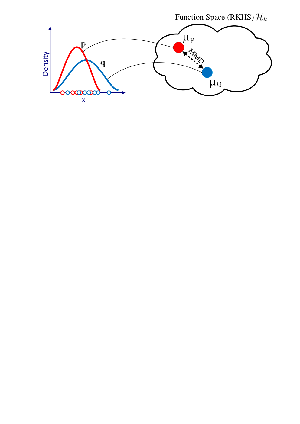
As shown in [25], the MMD in (4) can equivalently be expressed as

This gives an alternative interpretation of the MMD as the distance between mean embeddings in $\mathcal{H}_{k}$ as Fig. 2 illustrates.

A third expression for the MMD appears upon expanding the squared norm in (5) and using the reproducing property of $k$ which yields an expression in terms of $k$ as

The latter expression is computationally more appealing than the two former as it only calls for computation of expectations of the kernel. Thus, computation of the supremum in (4) is not required to compute the MMD. As discussed later in Section III-C, the expression (6) forms the basis for estimation of the MMD from data.

The choice of kernel defines the RKHS and thus the properties of its distance, the MMD. In addition to being reproducing, it is a great advantage if the kernel is characteristic [38, 39]. This implies that the kernel mean embedding is an injective mapping, meaning that each distribution is mapped to a unique function. Thus, in the case of characteristic kernels, the kernel mean embedding captures all the information about the distribution. As a result, $\mathrm{MMD}_{k}[\mathbb{P},\mathbb{Q}]=\|\mu_{\mathbb{P}}-\mu_{\mathbb{Q}}\|_{\mathcal{H}_{k}}=0$ if and only if $\mathbb{P}=\mathbb{Q}$. In this case, the MMD is capable of comparing infinitely many moments of two probability distributions without ever having to compute these moments explicitly. Consequently, the MMD is able to distinguish probability distributions even when these coincide in finite number of moments. This gives a great advantage over methods based on comparison of finitely many moments which are potentially blind to differences between distributions.

A very popular characteristic reproducing kernel is the squared-exponential (or Gaussian) kernel, defined as

for $\mathbf{x},\mathbf{x}^{\prime}\in\mathbb{R}^{d}$. Here, $\|\cdot\|_{2}$ is the Euclidean norm and $l>0$ is a parameter called the lengthscale of the kernel. The norm inside the exponent can be chosen based on the specific data and application. For additional examples of characteristic kernels, see [38, 39].

We now give a simple example comparing Gaussian distributions, in which case the MMD can be derived analytically.

Unlike in the previous example, it is, in most realistic cases, not feasible to analytically calculate (6). Moreover, numerical integration is problematic, as the dimension of $X$ and $Y$ may be large and $\mathbb{P}$ or $\mathbb{Q}$ unavailable. Fortunately, it is straightforward to estimate the MMD if it is an empirical distribution, such as in the case of data-sets.

Imagine that we do not have access to $\mathbb{P}$ and $\mathbb{Q}$, but that we instead have two data-sets consisting of realisations from these distributions. More precisely, suppose we have access to $\mathbf{X}=\{\mathbf{x}_{1},\dots,\mathbf{x}_{N_{X}}\}\overset{iid}{\sim}\mathbb{P}$ and $\mathbf{Y}=\{\mathbf{y}_{1},\dots,\mathbf{y}_{N_{Y}}\}\overset{iid}{\sim}\mathbb{Q}$. Then, an unbiased empirical estimate of $\mathrm{MMD}^{2}_{k}[\mathbb{P},\mathbb{Q}]$ can be obtained as [25]

Note that $N_{X}$ and $N_{Y}$ are permitted to differ, i.e. the two data-sets are not limited to be of the same size. To use this estimator with the kernel in (7), the lengthscale should be specified. Following [25], the lengthscale can be set based on the data-set $\mathbf{X}$ using the median heuristic

where $\mathrm{med}$ denotes the median of the set of squared two-norm distances $\|\mathbf{x}_{i}-\mathbf{x}_{j}\|_{2}^{2}$ for all pairs of distinct data points in $\mathbf{X}$. This setting of $l$ scales the kernel with the spread of the data, and is robust to outliers.

Concentration bounds for MMD, such as [26, Lemma 1] or [36, Theorem 3.4], imply that with high probability,

for some $C>0$. This tells us that the accuracy of the estimate converges linearly in both $N_{X}$ and $N_{Y}$. The computational cost of computing this estimate is $\mathcal{O}(N_{X}^{2}+N_{Y}^{2})$ due to the need to compute double sums in both $N_{X}$ and $N_{Y}$. In order to best balance computational cost and accuracy, $N_{X}$ and $N_{Y}$ should be chosen to be commensurate. These two results on accuracy and computational cost can be used to determine how to make default choices for the parameters of our ABC algorithm.

In order to use the MMD for calibrating stochastic radio channel models, we need a kernel defined on the space of transfer function measurements: $k_{\mathcal{Y}}:\mathcal{Y}\times\mathcal{Y}\rightarrow\mathbb{R}$. Given such a kernel, we could then estimate the MMD between a measured data-set $\mathbf{Y}$ and a data-set $\mathbf{Y}_{\mathrm{sim}}$ simulated from the model.

A significant challenge with this approach is that, in the context of stochastic radio channel models, $\mathcal{Y}$ is usually a high-dimensional space. This is especially the case for large bandwidth measurements where $N_{s}$ can be in the order of thousands. Such high-dimensional problems are challenging for kernel methods based on default kernels such as the squared-exponential kernel [41]. These kernels indeed suffer from the curse-of-dimensionality, a phenomenon implying that the distance between points increases exponentially with the dimension of the space.

To tackle this issue, there exist kernels specialised to certain time-series or functional data models in the literature [42, 43, 44, 45, 46, 47]. These use specific properties of the type of data in order to avoid the curse-of-dimensionality. In this paper, we contribute to this literature and construct a kernel specifically tailored to transfer function measurements. We base the kernel on the temporal moments of $y(t)$, defined as

The integral in (12) is easy to compute numerically. The temporal moments can be seen as an expansion of $|y(t)|^{2}$ into the basis of monomials. Since the monomials form a complete basis for finite energy time-limited signals [48], no information is lost compared to $|y(t)|^{2}$ if $I\rightarrow\infty$. Referring to [49, 50], the first few moments are well modeled by a log-normal distribution. Thus, taking the entry-wise logarithm $z^{(i)}=\ln m^{(0)}$ brings the moments to the same scale and gives an approximately Gaussian vector $\mathbf{z}=[z^{(0)},\dots,z^{(I-1)}]$. Multiple channel realizations yield $\mathbf{Z}=\left(\mathbf{z}_{1},\mathbf{z}_{2},\dots,\mathbf{z}_{N_{\mathrm{obs}}}\right)$.

Define the mapping $A_{I}:\mathcal{Y}\rightarrow\mathbb{R}^{I}$ from $\mathcal{Y}$ to the $I$-dimensional space of log temporal moments. We propose to construct a kernel $k_{\mathcal{Y}}$ for transfer function data as

where $k_{\text{SE}}$ denotes the squared-exponential kernel in dimension $I$. We note that this is the composition of a reproducing kernel and a map, and thus according to [51, Lemma 4.3] is a reproducing kernel on $\mathcal{Y}$. We also note that the MMD with kernel $k_{\mathcal{Y}}$ computed on the original data can be obtained through the MMD with kernel $k_{\text{SE}}$ on the log temporal moments. Similarly, the empirical estimators of these quantities are also identical, i.e.

where $\mathbf{X}$ is the simulated log temporal moments data-set.

In practice, we will have to limit ourselves to a finite $I$ for computational reasons. This, however, is not a problem since we can expect the signal energy to be concentrated on the lowest moments. In fact, taking $I$ to be small also allows us to by-pass issues with the curse-of-dimensionality.

From a theoretical viewpoint, since the squared-exponential kernel is characteristic, we should be able to recover any distribution on the space of log temporal moments. However, since the mapping $A_{I}$ leads to loss of information when $I$ is finite, $k_{\mathcal{Y}}$ will not be characteristic on $\mathcal{Y}$, and we may not be able to uniquely identify the distribution on $|y(t)|^{2}$. This however is not an issue for the considered channel models, as will be shown in Section V.

The proposed ABC method uses the MMD between data-sets as a rejection criteria. Instead of setting the threshold $\epsilon$ in terms of the distance, we specify the proportion of accepted samples, i.e. $\epsilon=M_{\epsilon}/M$ where $M_{\epsilon}$ is the number of parameter samples accepted out of $M$. This is particularly convenient as it avoids the need to manually find a threshold, which may lead to unknown run-time of the algorithm.

The method computes $\widehat{\mathrm{MMD}}_{k_{\text{SE}}}^{2}[\mathbf{X},\mathbf{Z}]$, where $\mathbf{X}=\left(\mathbf{x}_{1},\dots,\mathbf{x}_{N_{\mathrm{sim}}}\right)$ is the simulated log temporal moments data-set, as this is identical to estimating the MMD between $\mathbf{Y}$ and $\mathbf{Y}_{\mathrm{sim}}$ (see Eq. 14). First, $M$ independent parameter samples $\Theta=(\boldsymbol{\theta}_{1},\dots,\boldsymbol{\theta}_{M})$ are drawn from the prior $p(\boldsymbol{\theta})$. For each $\boldsymbol{\theta}_{i}$, the log temporal moments data-set, $\mathbf{X}_{i}\sim\mathbb{P}_{\boldsymbol{\theta}_{i}}$, is simulated. The simulated data-sets are gathered in $\mathcal{X}=\left(\mathbf{X}_{1},\dots,\mathbf{X}_{M}\right)$. The $\widehat{\mathrm{MMD}}_{k_{\text{SE}}}^{2}[\mathbf{X}_{i},\mathbf{Z}]$ is computed for each $i$ using (9), setting the lengthscale of $k_{\text{SE}}$ as per (10). The parameter samples resulting in the $M_{\epsilon}$ smallest MMD values are then accepted.

In principle, the MMD could be computed between the samples of the temporal moments instead of their logarithm. However, the magnitudes of the different temporal moments may vary strongly and using a single lengthscale may lead to poor performance. Using a log transformation helps mitigate this issue. Alternatively, the lengthscale should be defined for each dimension of $\boldsymbol{\theta}$.

As proposed in [53], it is possible improve the posterior approximation by adjusting the accepted samples using a model of the relationship between a low-dimensional vector of statistics and the parameter vector. Let $\mathbf{s}$ be a vector of summary statistics of $\mathbf{X}$ such that $\mathbf{s}=S(\mathbf{X})$ for a function $S(\cdot)$. Similarly, the observed summary statistics are denoted $\mathbf{s}_{\mathrm{obs}}=S(\mathbf{Z})$. We begin by fitting a function, $g$, between the accepted parameters $\Theta^{*}=(\boldsymbol{\theta}_{1}^{*},\dots,\boldsymbol{\theta}_{M_{\epsilon}}^{*})$ and the corresponding statistics $\mathcal{S}^{*}=(\mathbf{s}_{1},\dots,\mathbf{s}_{M_{\epsilon}})$ as [24, Ch. 3]

where $g(\mathbf{s})$ is the conditional expectation of $\boldsymbol{\theta}$ given $\mathbf{s}$, and $\varepsilon$ is the residual. Here, $\boldsymbol{\theta}$ should belong to a subset of $\mathbb{R}^{p}$. Considering that the log of the temporal moments are well modeled by a Gaussian distribution, we take $\mathbf{s}_{\mathrm{obs}}$ to be the vector consisting of the sample means and sample covariances of the elements of $\mathbf{z}$, similar to [22]. In total, $\mathbf{s}_{\mathrm{obs}}$ consists of $(I^{2}+3I)/2$ elements for $I$ temporal moments. The statistics $\mathbf{s}$ is computed in the same manner for $\mathbf{X}$. Note that $\mathbf{s}$ and $\mathbf{s}_{\mathrm{obs}}$ are normalized by an estimate of their median absolute deviation to account for the difference in magnitude of the statistics. In case the prior distributions are bounded, a logit transformation is applied to the parameters before the adjustment.

For simplicity reasons, we assume $g$ to be linear as in [53] and adjust the accepted parameters as

where $\hat{\boldsymbol{\beta}}$ is the solution to the weighted least-squares problem

The weighting function $\mathcal{W}$ applies weights to each $\boldsymbol{\theta}_{i}$ based on the estimated MMD value. This guarantees that parameters which yield simulated log moments “closer to” $\mathbf{Z}$ are weighted more heavily. We take $\mathcal{W}$ to be the Epanechnikov function, $\mathcal{W}_{(\delta)}=1-(\delta/\delta_{\mathrm{max}})^{2}$ for $|\delta|\leq\delta_{\mathrm{max}}$ and zero otherwise, as proposed in [53]. Here, $\delta_{\mathrm{max}}$ is the maximum estimated MMD associated to the accepted parameters. Note that choosing a constant regression function, i.e. $\boldsymbol{\beta}=0$, and assigning equal weights to all $\boldsymbol{\theta}_{i}$’s results in the basic rejection ABC algorithm. The regression adjustment therefore gives the adjusted parameter values $\tilde{\Theta}=(\tilde{\boldsymbol{\theta}}_{1},\dots,\tilde{\boldsymbol{\theta}}_{M_{\epsilon}})$.

As a means to explore the posterior distribution over the parameter space efficiently, we employ a sequential Monte Carlo technique called PMC [52, 20, 22]. In PMC, the current parameter values $\tilde{\Theta}$ are used to generate a new set of parameters for the next iteration of the algorithm through importance sampling. This is a two-step procedure: (1) sample from the current parameters based on their importance weights, and (2) perturb the sampled parameter values using a proposal density.

The set of parameters in the initial iteration, $\tilde{\Theta}^{(1)}=(\tilde{\boldsymbol{\theta}}_{1}^{(1)},\dots,\tilde{\boldsymbol{\theta}}_{M_{\epsilon}}^{(1)})$, are assigned equal weights. The next set of parameters is obtained by drawing $M$ values from $\tilde{\Theta}^{(1)}$ and perturbing these according to a probability distribution, called proposal. For simplicity, we perturb independently in each dimension using a Gaussian distribution, and reject values outside the prior range. Thus, the proposal reads

where $\mathbb{1}$ is an indicator function, $\mathcal{R}\subset\mathbb{R}^{p}$ is the prior range, and $\boldsymbol{\Sigma}$ is a diagonal matrix with variances $\sigma^{2}_{j}>0$ corresponding to parameter $\theta_{j}$ along the diagonal. We set the diagonal elements of $\boldsymbol{\Sigma}$ to twice the empirical variance of the adjusted parameter samples. This is denoted as $\boldsymbol{\Sigma}=2\widehat{\mathrm{Var}}(\tilde{\Theta})$.

The set of $M$ parameter values at iteration $t$, ${\Theta}^{(t)}$, is then used to simulate $\mathcal{X}^{(t)}$ from the model for MMD computation and regression adjustment (i.e. Alg. 1). In subsequent iterations, weights are assigned as

$j=1,\ldots,M_{\epsilon}$. The adjusted parameter values after iteration $T$ are taken as samples from the approximate posterior distribution. Point estimates of $\boldsymbol{\theta}$, such as the approximate posterior mean,

are straightforward to compute from the samples.

We have now completed the description of Alg. 2. However, the framework of ABC relies on the implicit assumption that there exist parameter values in the prior support that yield simulated data “close” to the measured data. This assumption may not always hold if the model parameters cannot be set in any way to reproduce the data well. In this case, we say that the model is misspecified for the data. Misspecification can be detected and accounted for in the algorithm as explained in this subsection.

Consider a univariate parameter $\theta$ in the range $[\theta_{\mathrm{min}},\theta_{\mathrm{max}}]$ resulting in a univariate statistic $s$ in $[s_{\mathrm{min}},s_{\mathrm{max}}]$ simulated from the model. If the observed statistic $s_{\mathrm{obs}}\notin[s_{\mathrm{min}},s_{\mathrm{max}}]$, then the model is likely to be misspecified. This is a challenge since under model misspecification, the local-linear regression adjustment has been shown to concentrate posterior mass on a completely different value than the rejection ABC [55]. In fact for parameters with bounded support, the regression adjustment moves the parameter samples outside the prior range as illustrated in Fig. 5. Hence, if $s_{\mathrm{obs}}$ lies outside the range of statistics that the model can simulate, then there is no guarantee that the adjusted samples of $\theta$ will lie inside the prior range.

We check for model misspecification by observing whether each element of $\mathbf{s}_{\mathrm{obs}}$ lies within the range of corresponding statistics simulated from the model using $\Theta^{(1)}$. If any element of $\mathbf{s}_{\mathrm{obs}}$ lies outside the range of values simulated from the model, then the model is deemed misspecified. In such a case, we replace $\mathbf{s}_{\mathrm{obs}}$ by an alternative term, $\breve{\mathbf{s}}_{\mathrm{obs}}$, computed from the model instead of the data using the parameter

where $f(\boldsymbol{\theta};\Theta^{*})$ is the kernel density estimate computed from the samples $\Theta^{*}$, and $\breve{\boldsymbol{\theta}}$ is the parameter corresponding to the mode of $f(\boldsymbol{\theta};\Theta^{*})$. Another choice for $\breve{\boldsymbol{\theta}}$ could be the posterior mean of rejection ABC [55]. However, we found the mean estimate to be unstable, especially in the initial iterations of the algorithm. Hence, in case of model misspecification, we set $\mathbf{s}_{\mathrm{obs}}=\breve{\mathbf{s}}_{\mathrm{obs}}$ in each iteration of the PMC-ABC algorithm, thus ensuring that the adjustment does not lead to parameter samples outside the prior range.

The seminal S-V model [2] is widely used as it is easy to simulate from, but is notoriously difficult to calibrate due to its structure. Even though the model can be analyzed using the theory of spatial point processes [57, 58] and moments derived [59], its likelihood function is unavailable. Recent discussions of the physical interpretation of the S-V model, also outlining some difficulties with the model calibration, is given in [60, 61, 62]. These difficulties have inspired the use of many different heuristic calibration methods, as outlined in the introduction.

In the S-V model, the multipath components are assumed to arrive in clusters. The arrival time of the clusters and that of the rays within the clusters are modeled as one-dimensional homogeneous Poisson point processes with arrival rates $\Lambda$ and $\lambda$, respectively. The gains of the multipath components are modeled as iid zero-mean complex Gaussian random variables with conditional variance that depends on three parameters; the average power of the first arriving multipath component $Q$, and the cluster and ray power decay constants $\Gamma,\gamma$, respectively. We refer the readers to [2] and [57] for a detailed description of the model. Including the noise variance, the parameter vector becomes $\boldsymbol{\theta}=[Q,\Lambda,\lambda,\Gamma,\gamma,\sigma_{W}^{2}]^{\top}$.

We begin by finding a reasonable value of $N_{\mathrm{sim}}$. To that end, we generate pseudo-observed log moments, $\mathbf{X}_{\mathrm{true}}$, with $N_{\mathrm{obs}}=1000$ realizations from the model by setting $\boldsymbol{\theta}$ to a “true” value. Using another value of the parameter vector, say $\boldsymbol{\theta}^{\prime}$, we simulate $\mathbf{X}^{\prime}$ from the model with varying $N_{\mathrm{sim}}$ and compute the estimated MMD between $\mathbf{X}^{\prime}$ and $\textbf{X}_{\text{true}}$. This process is repeated $100$ times to create error bars as shown in Fig. 6. Although the MMD estimate gets more accurate as $N_{\mathrm{sim}}$ increases, the improvement however is small. Choosing a higher $N_{\mathrm{sim}}$ improves the MMD estimate, but increases the run-time of the of the algorithm significantly (since the computational cost is quadratic in $N_{\mathrm{sim}}$, and simulating from the model can also be slow). Therefore, we set $N_{\mathrm{sim}}=100$ as a reasonable compromise considering the trade-off between accuracy and computational cost.

We first verify that the MMD computed from the temporal moments reacts to changes in the S-V model parameters. To that end, we generate simulated data-sets by varying one parameter uniformly in the prior support while keeping the others fixed to their true value. As can be seen from Fig. 7, the estimated MMD values increase as each of the parameters move away from their true value, and the minimum is (approximately) achieved when both the data-sets are generated from approximately the same parameters. The MMD reacts to changes in all the parameters, albeit more for some than others, as can be seen from the different scales of the y-axis. We therefore conclude that the distribution of the first four log temporal moments is informative about the S-V model parameters.

We now use the proposed method to calibrate the S-V model using $\mathbf{X}_{\mathrm{true}}$. We assume uninformative (flat) priors in the range given in Tab. I for all the parameters to ensure that their marginal posteriors are unaffected by any prior beliefs. The prior ranges were set according to the measurement settings as done in [20]. The plots indicating convergence of the algorithm and the marginal posterior distributions for $T=10$ iterations are shown in Fig. 8. The approximate posterior samples concentrate around the true value for all the parameters. The algorithm converges rather quickly and the posteriors taper as the iterations proceed. In principle, the iterations could be stopped after four or five iterations, but we let it run till $T=10$ for clarity. The algorithm gives a reasonable estimate for the parameters even in the first iteration. The proposed method is able to estimate $\Lambda$ accurately as well, unlike in [20] where some post-processing was required to estimate $\Lambda$.

As our second example, we demonstrate the performance of our proposed method on the PG model. The PG model was first introduced in [63], and since then has been applied to a wide range of scenarios in [64, 65, 66, 67]. Recently, it has been extended to account for polarization in [68, 15, 69]. Although the model is easy to simulate from, its likelihood function is unknown. A method of moments based estimator was applied to calibrate the model in [15], but the moments equations were based on approximation and it required manually fixing one of the parameters.

The PG model [63] represents the radio channel as a directed graph with the transmitters, receivers and scatterers as vertices. Edges model the wave propagation between the vertices. Edges are defined randomly depending on the probability of visibility, $P_{\mathrm{vis}}$. Other parameters of the model include the number of scatterers, $N_{\mathrm{scat}}$, and the reflection gain, $g$, resulting in the parameter vector $\boldsymbol{\theta}=[g,N_{\mathrm{scat}},P_{\mathrm{vis}},\sigma_{W}^{2}]^{\top}$. Note that $N_{\mathrm{scat}}$ is assumed to be real-valued during the regression adjustment, following which, its adjusted samples are rounded off to the nearest integer. We used the antenna positions and room geometry for the model according to the measurement conditions given in [56]. Hence, $N_{\mathrm{obs}}=N_{\mathrm{sim}}=625$ for the PG model. For each call of the model, the scatterer positions are drawn uniformly across the room, and all 625 realizations are generated based on those positions.

We again use uniform priors for the parameters (see Tab. I) and apply $T=10$ iterations of the proposed method to calibrate the PG model to the pseudo-observed data-set generated from $\boldsymbol{\theta}_{\mathrm{true}}$. To prevent biased results due to a particular configuration of the scatterers, we generate the pseudo-observed data by combining data from four different calls of the model using $\boldsymbol{\theta}_{\mathrm{true}}$. From Fig. 11, we observe that the algorithm converges very quickly, and gives posteriors which are highly concentrated around the true value for $P_{\mathrm{vis}}$, $N_{\mathrm{scat}}$, and $\sigma_{W}^{2}$. The approximate posterior for $g$ starts off very wide and then gets narrower as the iterations proceed. The method is therefore able to accurately calibrate the PG model.

To asses how the performance of the proposed algorithm is affected by the presence of noise, we now repeat this simulation experiment for different noise levels. We fix $g=0.6$, $P_{\mathrm{vis}}=0.5$, $N_{\mathrm{scat}}=15$ and vary $\sigma^{2}_{W}$ from $10^{-10}$ to $10^{-6}$. The signal-to-noise ratio (SNR), is defined as

where $\bar{m}_{0}$ is the sample mean of of the zeroth temporal moment computed by setting $\sigma^{2}_{W}=0$ in the PG model. The resulting averaged power delay profile (APDP) is shown in Fig. 9. We run $T=10$ iterations of the algorithm for each of the SNR values. The prior for $\sigma^{2}_{W}$ is adjusted according to the true value in each run of the algorithm. The violin plots of the approximate posterior after the tenth iteration in each case is shown in Fig. 10.

We observe that the noise variance $\sigma^{2}_{W}$ is estimated extremely accurately at each SNR level. The estimation accuracy for $P_{\mathrm{vis}}$ and $N_{\mathrm{scat}}$ seems to suffer only at the lowest SNR level. Reducing the SNR impacts the estimation accuracy of $g$ the most, with its approximate posterior converging to the prior as SNR decreases. This is expected as the higher the noise variance, the less visible the slope of the power delay profile which is determined by $g$. In conclusion, the algorithm performs well at SNR values encountered in measurements.

Upon applying Alg. 2 to the measured data, regression adjustment yielded parameter samples outside the prior range. This indicated that the model is misspecified. That is indeed evident from Fig. 12 where we plot elements of the vector $\mathbf{s}$, namely the mean and variance of $\mathbf{z}_{0}$ and $\mathbf{z}_{1}$, obtained from the measurements and the S-V model. The simulated summaries correspond to 2000 parameter values drawn from the prior. We observe that varying the parameters of the S-V model in the prior range generated mean values that overlap the mean value from the measurements. However, the variance values from the S-V model does not capture the value observed in the measurements. That is, there exists no such $\boldsymbol{\theta}$ in the prior range that leads to $\mathbf{s}$ “close” to $\mathbf{s}_{\mathrm{obs}}$ in terms of the variance of the temporal moments. Hence, the model is misspecified for this data and so we obtain $\mathbf{s}_{\mathrm{obs}}$ from the model as per Sec. IV-D.

The posteriors obtained from the measured data are shown in Fig. 13 for $T=15$ iterations. The marginal approximate posteriors for $\lambda$, $\Gamma$, and $\sigma^{2}_{W}$ are highly concentrated. Posteriors for $\Gamma$ and $\sigma^{2}_{W}$ appear to converge from the second iteration itself, indicating that these parameters affect the MMD the most. The posterior for $\lambda$ becomes narrow and converges after the first few iterations. The posteriors for $Q$, $\Lambda$ and $\gamma$ take around eight or nine iterations to converge to a different location in the prior range than where they began from, unlike the simulation experiment. This is potentially due to the model being misspecified for the data, and so parameters that affect the distribution of the log temporal moments the most converge first. The approximate estimates after 15 iterations are reported in Tab. I. Considering that the regression adjustment in the first few iterations are done based on a coarse estimate of $\mathbf{s}_{\mathrm{obs}}$ from the model, the algorithm seems to work very well. The estimate of $\Lambda$ is high, indicating arrival of around 17 clusters on an average, while that of $\lambda$ is quite low. The model is therefore forced to the case with many clusters having very few multipath components each, thus approaching the “unclustered” Turin model with constant rate.

The misspecification of the S-V model for the measured data is not surprising, as the measurement conditions are not replicated in the model. The virtual array measurements are from a single array position in the room, hence the same clusters are observed in each transmit-receive antenna pair. On the other hand, each realization out of the S-V model is an independent realization from the underlying point process. As a result, we hardly see any variance in the log temporal moments of the data, which is not achieved in the S-V model for any configuration of the parameters.

The results obtained on calibration of the PG model on measured data after $T=10$ iterations is shown in Fig. 14. In this case, the model is not misspecified for the considered data. The approximate marginal posterior distributions for all the parameters start off wide and then seem to converge after around four or five iterations. The posteriors are also quite concentrated for all the four parameters, especially $P_{\mathrm{vis}}$ and $\sigma^{2}_{W}$. Overall, the results are similar to what is observed in the simulation experiment. See Tab. I for approximate estimates of the parameters after $T=10$ iterations. The estimates are very similar to the ones reported in [22] where the polarized PG model was calibrated on data from the same measurement campaign. The estimate of $P_{\mathrm{vis}}$ is almost one, indicating that nearly all scatterers are connected. The estimates of $g$ and $P_{\mathrm{vis}}$ are consistent with the values reported from measurements [15] in other in-room scenarios for the PG model. Moreover, these values are close to those used in simulations with the PG model in [70, 63].

While the proposed method easily calibrates both the S-V and the PG models to measured data, there is no guarantee that the fitted models replicate the data well. This effect is of course not specific to the proposed method, but pertains to any calibration method. Thus, an extra step, termed model validation, should be performed where predictions of the calibrated models are compared to the data, and possibly other data-sets not used in the calibration process. Performing a full model validation is out of scope of this paper, as our focus is on the calibration method itself. Instead, as a final step we check how well the two calibrated models fit the input data-set.

To this end, we simulate 625 channel realizations from both models with parameters set according to Tab. I. We compare the outputs from the models to the measured data in terms of the APDP and the empirical cumulative distribution function (cdf) of root mean square (rms) delay spread $\tau_{\mathrm{rms}}$, mean delay $\bar{\tau}$, and received power $P_{0}$ computed per channel realization, according to

It appears from Fig. 15 that both the models are able to fit the APDP of the measurements well. The slope is captured well by both the models, along with the noise floor, although the S-V model slightly underestimates it. The S-V model, however, is not able to replicate the peaks in the APDP of the measurements, while the PG model represents the initial peaks better. This effect is to be expected for the particular settings of the S-V model with many clusters and very few within-cluster components. The peaks from the S-V model are averaged out since the channel realizations are independent. This is unlike the PG model where positions of the antennas in the virtual array are included, thus simulating correlated channel realizations.

Even though the APDPs are similar, the two models yields very different empirical cdfs of $\tau_{\mathrm{rms}}$, $\bar{\tau}$, and $P_{0}$ as reported in Fig. 15. The PG model captures the behavior of the cdfs very well, while the S-V model clearly fails to do so, especially for the mean delay and the received power. The means of the rms delay spread from both the models are fairly close to the measured data, but the spread differs for the S-V model. As noticed theoretically in [61, 62], multipath models can yield temporal moments with similar means while differing vastly in variance. Indeed, for a stochastic multipath model, the covariance structure of the temporal moments depends on both first- and second-order properties of the underlying point process [71].

The misspecification of the S-V model arises from disregarding the dependencies between the measurements obtained from different antennas in the array. This in turn leads to the discrepancy in the variance of the log temporal moments as observed in Fig 12. Thus, to alleviate the misspecification, the array structure should be incorporated in the model, as is done inherently in the PG model. This could be a contributing reason why other authors [72] have found fully stochastic models inadequate and instead recommended using geometry-based and fully deterministic approaches for millimetre-wave data. Irrespective of the cause, such misspecifications can be detected by the proposed method, thereby assisting in the modeling process.

References

- [1] G. L. Turin, F. D. Clapp, T. L. Johnston, S. B. Fine, and D. Lavry, “A statistical model of urban multipath propagation,” IEEE Trans. Veh. Technol., vol. 21, pp. 1–9, Feb 1972.
- [2] A. A. M. Saleh and R. Valenzuela, “A statistical model for indoor multipath propagation,” IEEE J. Sel. Areas Commun., vol. 5, pp. 128–137, February 1987.
- [3] K. Haneda, J. Järveläinen, A. Karttunen, M. Kyrö, and J. Putkonen, “A statistical spatio-temporal radio channel model for large indoor environments at 60 and 70 GHz,” IEEE Trans. Antennas Propag., vol. 63, no. 6, pp. 2694–2704, 2015.
- [4] L. Raschkowski, P. Kyösti, K. Kusume, and E. T. Jämsä, METIS channel models, deliverable D1.4 V3.
- [5] P. Kyösti, WINNER II channel models, deliverables D1.1.2 V1.2, part I: Channel models.
- [6] C. Gustafson, K. Haneda, S. Wyne, and F. Tufvesson, “On mm-wave multipath clustering and channel modeling,” IEEE Trans. Antennas Propag., vol. 62, no. 3, pp. 1445–1455, 2014.
- [7] J. Poutanen, K. Haneda, L. Liu, C. Oestges, F. Tufvesson, and P. Vainikainen, “Parameterization of the COST 2100 MIMO channel model in indoor scenarios,” in Eur. Conf. on Antennas and Propag., pp. 3606–3610, 2011.
- [8] J. Li, B. Ai, R. He, M. Yang, Z. Zhong, and Y. Hao, “A cluster-based channel model for massive mimo communications in indoor hotspot scenarios,” IEEE Trans. on Wireless Commun., vol. 18, no. 8, pp. 3856–3870, 2019.
- [9] M. Yang, B. Ai, R. He, G. Wang, L. Chen, X. Li, C. Huang, Z. Ma, Z. Zhong, J. Wang, Y. Li, and T. Juhana, “Measurements and cluster-based modeling of vehicle-to-vehicle channels with large vehicle obstructions,” IEEE Trans. on Wireless Commun., vol. 19, no. 9, pp. 5860–5874, 2020.
- [10] X. Yin and X. Cheng, Propagation Channel Characterization, Parameter Estimation, and Modeling for Wireless Communications. John Wiley & Sons Singapore Pte. Ltd, Feb 2018.
- [11] N. Czink, P. Cera, J. Salo, E. Bonek, J. P. Nuutinen, and J. Ylitalo, “A framework for automatic clustering of parameteric MIMO channel data including path powers,” in Proc. IEEE 64th Veh. Technol. Conf.-Fall, pp. 1–5, 2006.
- [12] C. Gentile, “Using the kurtosis measure to identify clusters in wireless channel impulse responses,” IEEE Trans. Antennas Propag., vol. 61, no. 6, pp. 3392–3396, 2013.
- [13] R. He, W. Chen, B. Ai, A. F. Molisch, W. Wang, Z. Zhong, J. Yu, and S. Sangodoyin, “On the clustering of radio channel impulse responses using sparsity-based methods,” IEEE Trans. Antennas Propag., vol. 64, no. 6, pp. 2465–2474, 2016.
- [14] L. Greenstein, S. Ghassemzadeh, S.-C. Hong, and V. Tarokh, “Comparison study of UWB indoor channel models,” IEEE Trans. on Wireless Commun., vol. 6, pp. 128–135, Jan 2007.
- [15] R. Adeogun, T. Pedersen, C. Gustafson, and F. Tufvesson, “Polarimetric Wireless Indoor Channel Modelling Based on Propagation Graph,” IEEE Trans. on Antennas and Propag., vol. 67, no. 10, pp. 6585–6595, 2019.
- [16] C. Hirsch, A. Bharti, T. Pedersen, and R. Waagepetersen, “Maximum likelihood calibration of stochastic multipath radio channel models,” IEEE Trans. on Antennas and Propag., pp. 1–1, 2020.
- [17] A. Bharti, R. Adeogun, and T. Pedersen, “Parameter Estimation for Stochastic Channel Models using Temporal Moments,” in Proc. 2019 IEEE Int. Symp. on Antennas and Propag. and USNC-URSI Radio Sci. Meeting, pp. 1267–1268, 2019.
- [18] W.-D. Wu, C.-H. Wang, C.-C. Chao, and K. Witrisal, “On parameter estimation for ultra-wideband channels with clustering phenomenon,” in IEEE 68th Veh. Technol. Conf., IEEE, Sep 2008.
- [19] A. Bharti, R. Adeogun, and T. Pedersen, “Estimator for Stochastic Channel Model without Multipath Extraction using Temporal Moments,” in 20th IEEE Int. Workshop on Signal Process. Advances in Wireless Commun. (SPAWC), pp. 1–5, 2019.
- [20] A. Bharti and T. Pedersen, “Calibration of stochastic channel models using approximate Bayesian computation,” in Proc. IEEE Global Commun. Conf. Workshops, pp. 1–6, 2019.
- [21] R. Adeogun, “Calibration of stochastic radio propagation models using machine learning,” IEEE Antennas and Wireless Propag. Lett., vol. 18, pp. 2538–2542, Dec 2019.
- [22] A. Bharti, R. Adeogun, and T. Pedersen, “Learning parameters of stochastic radio channel models from summaries,” IEEE Open J. of Antennas and Propag., vol. 1, pp. 175–188, 2020.
- [23] A. Bharti, R. Adeogun, and T. Pedersen, “Auto-generated summaries for stochastic radio channel models,” in 15th Eur. Conf. on Antennas and Propag., pp. 1–5, 2021.
- [24] S. A. Sisson, Handbook of Approximate Bayesian Computation. Chapman and Hall/CRC, Sep 2018.
- [25] A. Gretton, K. Borgwardt, M. J. Rasch, and B. Scholkopf, “A kernel two-sample test,” J. of Mach. Learn. Res., vol. 13, pp. 723–773, 2012.
- [26] F.-X. Briol, A. Barp, A. B. Duncan, and M. Girolami, “Statistical inference for generative models with maximum mean discrepancy,” arXiv:1906.05944, 2019.
- [27] B.-E. Chérief-Abdellatif and P. Alquier, “Finite sample properties of parametric MMD estimation: robustness to misspecification and dependence,” arXiv:1912.05737, 2020.
- [28] B.-E. Cherief-Abdellatif and P. Alquier, “MMD-Bayes: Robust bayesian estimation via maximum mean discrepancy,” vol. 118 of Proc. of Mach. Learn. Res., pp. 1–21, PMLR, 08 Dec 2020.
- [29] S. Nakagome, K. Fukumizu, and S. Mano, “Kernel approximate Bayesian computation in population genetic inferences,” Stat. Appl. in Genet. and Mol. Biol., vol. 12, no. 6, pp. 667–678, 2013.
- [30] M. Park, W. Jitkrittum, and D. Sejdinovic, “K2-ABC: approximate Bayesian computation with kernel embeddings,” Proc. of the 19th Int. Conf. on Artif. Intell. and Statistics, vol. 51, pp. 398–407, 2015.
- [31] J. Mitrovic, D. Sejdinovic, and Y. W. Teh, “DR-ABC: Approximate Bayesian computation with kernel-based distribution regression,” 33rd Int. Conf. on Mach. Learn., ICML, vol. 3, pp. 2209–2218, 2016.
- [32] K. Kisamori, M. Kanagawa, and K. Yamazaki, “Simulator calibration under covariate shift with kernels,” in Proc.s of the 23rd Int. Conf. on Artif. Intell. and Statistics, vol. 108, pp. 1244–1253, PMLR, Aug 2020.
- [33] G. K. Dziugaite, D. M. Roy, and Z. Ghahramani, “Training generative neural networks via maximum mean discrepancy optimization,” in Proc. of 31st Conf. on Uncertain. in Artif. Intell., pp. 258–267, 2015.
- [34] D. J. Sutherland, H.-Y. Tung, H. Strathmann, S. De, A. Ramdas, A. Smola, and A. Gretton, “Generative models and model criticism via optimized maximum mean discrepancy,” in Int. Conf. on Learn. Represent., 2017.
- [35] Y. Li, K. Swersky, and R. Zemel, “Generative moment matching networks,” in Proc. of the 32nd Int. Conf. on Mach. Learn. - Vol. 37, ICML’15, p. 1718–1727, JMLR.org, 2015.
- [36] K. Muandet, K. Fukumizu, B. Sriperumbudur, and B. Schölkopf, “Kernel mean embedding of distributions: A review and beyond,” Found. and Trends in Mach. Learn., vol. 10, no. 1-2, pp. 1–141, 2017.
- [37] A. Berlinet and C. Thomas-Agnan, Reproducing Kernel Hilbert Spaces in Probability and Statistics. New York: Springer Science+Business Media, 2004.
- [38] B. K. Sriperumbudur, A. Gretton, K. Fukumizu, B. Schölkopf, and G. R. G. Lanckriet, “Hilbert space embeddings and metrics on probability measures,” J. of Mach. Learn. Res., vol. 11, 2010.
- [39] C.-J. Simon-Gabriel and B. Schölkopf, “Kernel Distribution Embeddings: Universal Kernels, Characteristic Kernels and Kernel Metrics on Distributions,” J. of Mach. Learn. Res., vol. 19, no. 44, pp. 1–29, 2018.
- [40] F.-X. Briol, C. J. Oates, M. Girolami, and M. A. Osborne, “Frank-wolfe bayesian quadrature: Probabilistic integration with theoretical guarantees,” in Proc. of the 28th Int. Conf. on Neural Inf. Process. Syst. - Volume 1, NIPS’15, p. 1162–1170, 2015.
- [41] S. Reddi, A. Ramdas, B. Poczos, A. Singh, and L. Wasserman, “On the High Dimensional Power of a Linear-Time Two Sample Test under Mean-shift Alternatives,” in Proc. of the 18th Int. Conf. on Artif. Intell. and Stat., vol. 38, pp. 772–780, PMLR, May 2015.
- [42] S. Rüping, “SVM kernels for time series analysis,” tech. rep., 2001.
- [43] M. Cuturi, J.-P. Vert, Ø. Birkenes, and T. Matsui, “A kernel for time series based on global alignments,” IEEE Int. Conf. on Acoust,, Speech and Signal Process., vol. 2, pp. 413–416, 2007.
- [44] M. Cuturi, “Fast global alignment kernels,” Proc. of the 28th Int. Conf. on Mach. Learn., pp. 929–936, 2011.
- [45] I. Chevyrev and H. Oberhauser, “Signature moments to characterize laws of stochastic processes,” arXiv:1810.10971, 2018.
- [46] F. J. Kiŕaly and H. Oberhauser, “Kernels for sequentially ordered data,” J. of Mach. Learn. Res., vol. 20, pp. 1–45, 2019.
- [47] G. Wynne and A. B. Duncan, “A kernel two-sample test for functional data,” arXiv:2008.11095, 2020.
- [48] L. E. Franks, Signal Theory. Englewood Cliffs, N. J., Prentice-Hall, 1969.
- [49] A. Bharti, L. Clavier, and T. Pedersen, “Joint statistical modeling of received power, mean delay, and delay spread for indoor wideband radio channels,” in 14th Eur. Conf. on Antennas and Propag., pp. 1–5, 2020.
- [50] A. Bharti, R. Adeogun, X. Cai, W. Fan, F.-X. Briol, L. Clavier, and T. Pedersen, “Joint modeling of received power, mean delay, and delay spread for wideband radio channels,” IEEE Trans. on Antennas and Propag., pp. 1–1, 2021.
- [51] I. Steinwart and A. Christmann, Support Vector Machines. Springer, 2008.
- [52] M. A. Beaumont, J.-M. Cornuet, J.-M. Marin, and C. P. Robert, “Adaptive approximate bayesian computation,” Biometrika, vol. 96, pp. 983–990, Oct 2009.
- [53] M. A. Beaumont, W. Zhang, and D. J. Balding, “Approximate bayesian computation in population genetics,” Genetics, vol. 162, no. 4, pp. 2025–2035, 2002.
- [54] J. Lintusaari, M. U. Gutmann, R. Dutta, S. Kaski, and J. Corander, “Fundamentals and recent developments in approximate bayesian computation,” Syst. Biol., vol. 66, pp. 66–82, Jan 2017.
- [55] D. T. Frazier, C. P. Robert, and J. Rousseau, “Model misspecification in approximate bayesian computation: consequences and diagnostics,” J. of the R. Stat. Soc.: Ser. B (Stat. Methodol.), vol. 82, pp. 421–444, Jan 2020.
- [56] C. Gustafson, D. Bolin, and F. Tufvesson, “Modeling the polarimetric mm-wave propagation channel using censored measurements,” in 2016 Global Commun. Conf., IEEE, Dec 2016.
- [57] M. L. Jakobsen, T. Pedersen, and B. H. Fleury, “Analysis of the stochastic channel model by saleh & valenzuela via the theory of point processes,” Int. Zurich Seminar on Commun., 2012.
- [58] J. A. Gubner, B. N. Bhaskar, and K. Hao, “Multipath-cluster channel models,” in 2012 IEEE Int. Conf. on Ultra-Wideband, pp. 292–296, 2012.
- [59] M. S. Derpich and R. Feick, “Second-order spectral statistics for the power gain of wideband wireless channels,” IEEE Trans. on Veh. Technol., vol. 63, no. 3, pp. 1013–1031, 2014.
- [60] A. Meijerink and A. F. Molisch, “On the physical interpretation of the saleh–valenzuela model and the definition of its power delay profiles,” IEEE Trans. on Antennas and Propag., vol. 62, no. 9, pp. 4780–4793, 2014.
- [61] T. Pedersen, “Modeling of path arrival rate for in-room radio channels with directive antennas,” IEEE Trans. on Antennas and Propag., vol. 66, no. 9, pp. 4791–4805, 2018.
- [62] T. Pedersen, “Stochastic Multipath Model for the In-Room Radio Channel Based on Room Electromagnetics,” IEEE Trans. on Antennas and Propag., vol. 67, pp. 2591–2603, April 2019.
- [63] T. Pedersen and B. H. Fleury, “Radio channel modelling using stochastic propagation graphs,” in IEEE ICC, pp. 2733–2738, June 2007.
- [64] L. Tian, X. Yin, Q. Zuo, J. Zhou, Z. Zhong, and S. X. Lu, “Channel modeling based on random propagation graphs for high speed railway scenarios,” in IEEE PIMRC, pp. 1746–1750, Sept 2012.
- [65] L. Tian, V. Degli-Esposti, E. M. Vitucci, and X. Yin, “Semi-deterministic radio channel modeling based on graph theory and ray-tracing,” IEEE Trans. on Antennas and Propag., vol. 64, pp. 2475–2486, June 2016.
- [66] J. Chen, X. Yin, L. Tian, and M. Kim, “Millimeter-wave channel modeling based on a unified propagation graph theory,” IEEE Commun. Lett., vol. 21, pp. 246–249, Feb 2017.
- [67] R. O. Adeogun, A. Bharti, and T. Pedersen, “An iterative transfer matrix computation method for propagation graphs in multi-room environments,” IEEE Antennas and Wireless Propag. Lett., vol. 18, pp. 616–620, April 2019.
- [68] R. Adeogun and T. Pedersen, “Propagation graph based model for multipolarized wireless channels,” in IEEE WCNC, April 2018.
- [69] R. Adeogun and T. Pedersen, “Modelling polarimetric power delay spectrum for indoor wireless channels via propagation graph formalism,” in 2nd URSI Atlantic Radio Sci. Meeting, May 2018.
- [70] T. Pedersen, G. Steinböck, and B. H. Fleury, “Modeling of reverberant radio channels using propagation graphs,” vol. 60, pp. 5978–5988, Dec 2012.
- [71] T. Pedersen, “First- and second order characterization of temporal moments of stochastic multipath channels,” in 2020 33rd Gen. Assembly and Sci. Symp. of the Int. Union of Radio Sci., pp. 1–4, 2020.
- [72] S. Salous, V. D. Esposti, F. Fuschini, R. S. Thomae, R. Mueller, D. Dupleich, K. Haneda, J.-M. M. Garcia-Pardo, J. P. Garcia, D. P. Gaillot, S. Hur, and M. Nekovee, “Millimeter-wave propagation: Characterization and modeling toward fifth-generation systems. [wireless corner],” IEEE Antennas and Propagation Magazine, vol. 58, pp. 115–127, dec 2016.
- [73] A. Barp, F.-X. Briol, A. Duncan, M. Girolami, and L. Mackey, “Minimum stein discrepancy estimators,” in Adv. in Neural Inform. Process. Syst., vol. 32, pp. 12964–12976, 2019.
![[Uncaptioned image]](2012.09612v2/ab.png) |
Ayush Bharti received the B.E. degree in electrical and electronics engineering from Birla Institute of Technology and Sciences, Pilani, India, in 2015, and the M.Sc. degree in signal processing and computing from Aalborg University, Denmark, in 2017, where he is currently pursuing the Ph.D. with the Department of Electronic Systems. His research interests include likelihood-free inference, statistical signal processing, and radio channel modeling. |
![[Uncaptioned image]](2012.09612v2/fxbriol_photo.jpg) |
François-Xavier Briol received a Bachelor with integrated Masters in Mathematics, Operational Research, Statistics and Economics (MMORSE) in 2014, then a PhD in Statistics in 2019, both from the University of Warwick. He was briefly a research associate at Imperial College London and the University of Cambridge, before joining University College London (UCL) in 2019 where he is now a Lecturer in Statistical Science. Dr. Briol is also a Group Leader in Data-Centric Engineering at The Alan Turing Institute, the UK’s national institute for Data Science and AI, where he currently leads a project on “Fundamentals of Statistical Machine Learning”. His research interests include statistical computation and inference for large scale and computationally expensive probabilistic models. |
![[Uncaptioned image]](2012.09612v2/troels_300x400.png) |
Troels Pedersen received the M.Sc. degree in digital communications and the Ph.D. degree in wireless communications from Aalborg University, Aalborg, Denmark, in 2004 and 2009, respectively. In 2005, he was a Guest Researcher with the FTW Telecommunications Research Center Vienna, Vienna, Austria. He joined the Department of Electronic Systems, Aalborg University, as an Assistant Professor, in 2009, and became an Associate Professor in 2012. In 2012, he was a Visiting Professor with the Institut d’Électronique et de Télécommunications de Rennes, University of Rennes 1, Rennes, France. His current research interests include statistical signal processing and communication theory, including sensor array signal processing, radio geolocation techniques, radio channel modeling, and radio channel sounding. Dr. Pedersen received the Teacher of the Year Award from the Study Board for Electronics and IT, Aalborg University, in 2011 and 2017. |