Solving large permutation flow-shop scheduling problems on GPU-accelerated supercomputersJournal: Journal of LaTeX Templates
Abstract
Makespan minimization in permutation flow-shop scheduling is a well-known hard combinatorial optimization problem. Among the standard benchmark instances proposed by E. Taillard in 1993, have remained unsolved for almost three decades. In this paper, we present our attempts to solve these instances to optimality using parallel Branch-and-Bound tree search on the GPU-accelerated Jean Zay supercomputer. We report the exact solution of previously unsolved problem instances and improved upper bounds for instances. The solution of these problems requires both algorithmic improvements and leveraging the computing power of peta-scale high-performance computing platforms. The challenge consists in efficiently performing parallel depth-first traversal of a highly irregular, fine-grained search tree on distributed systems composed of hundreds of massively parallel accelerator devices and multi-core processors. We present and discuss the design and implementation of our permutation-based B&B and experimentally evaluate its parallel performance on up to 384 V100 GPUs (2 million CUDA cores) and 3840 CPU cores. The optimality proof for the largest solved instance requires about CPU-years of computation —using GPUs and over million parallel search agents, the traversal of the search tree is completed in hours, exploring nodes.
Keywords:
Permutation flow-shop scheduling , Branch-and-Bound , Supercomputing , GPU computing1 Introduction
Many combinatorial optimization problems (e.g. scheduling, assignment or routing problems) can be modeled by using permutations to represent candidate solutions. In this work, we focus on the Permutation Flowshop Scheduling Problem (PFSP) with makespan criterion. The problem consists in scheduling jobs in identical order on machines, given the processing times for job on machine and the constraint that a job can only start on machine if it is completed on all upstream machines . The goal is to find a permutation (a processing order) that minimizes the completion time of the last job on the last machine, called makespan.
The problem is NP-hard for [1] and exact algorithms like Branch-and-Bound (BB) can only solve small-sized instances within a reasonable amount of time. BB performs an implicit enumeration of all possible solutions by dynamically constructing and exploring a tree. This is done using four operators: branching, bounding, selection and pruning. For larger problem instances, the exhaustive exploration of the search space becomes practically infeasible on a sequential computer. In this article, we present PBBCluster, a permutation-based BB (PBB) algorithm for heterogeneous clusters composed of multi-core processors and GPU accelerator devices. Scaling PBBCluster on hundreds of GPUs of the Jean Zay supercomputer (#57 in the Top500 ranking, Nov. 2020), we aim at solving hard PFSP benchmark instances to optimality that remained open for almost three decades.
Our motivation is twofold. On the one hand, the knowledge of exact optimal solutions for benchmark instances is highly valuable, as they provide a baseline for assessing the quality of metaheuristics and other approximate methods. In the case of the PFSP, the set of benchmark instances proposed by E. Taillard in 1993 [2] is the most frequently used. While instances defined by less than machines are relatively easy to solve [3], most of Taillard’s instances with machines and jobs are very hard and optimal solutions for of them remain unknown years after their introduction.
On the other hand, the efficient parallel design and implementation of backtracking/BB algorithms is challenging, mainly because this “computational dwarf"[4] is highly irregular. Moreover, the efficient design of parallel BB is strongly influenced by the tackled problem (search space, goal and granularity) and on the targeted compute platform [5]. The potential for exploiting parallelism in BB has been recognized as early as 1975 and research activity started to intensify ten years later, as parallel processing capabilities became practically available [6]. A survey which covers the main research lines on parallel BB from 1975 to 1994 may be found in [7]. To place this article in a historical context, it could be useful to point out two particularly fruitful research phases.
In the early 1990s, the design of massively parallel tree-search algorithms on top of SIMD supercomputers (MasPar, CM-2, Intel Hypercube, etc.) has attracted much attention [8, 9], with research interests focusing on data-parallel load balancing strategies [10, 11]. Frequently used applications include puzzles (e.g. 15-puzzle) and games (e.g. Othello), which are characterized by regular fine-grained evaluation functions and highly irregular search trees. Notably, backtracking and BB algorithms for modern GPUs are designed similarly, and many GPU-based parallel tree-search algorithms target fine-grained applications as well [12, 13, 14].
A decade later, with the emergence of cluster and grid computing, research focus shifted towards the design of parallel BB algorithms on top of distributed, heterogeneous and volatile platforms, targeting more coarse-grained applications of BB [15]. The use of well-engineered grid-enabled BB algorithms has led to breakthroughs such as the resolution, in 2002, of quadratic assignment problem (QAP) instances which had remained unsolved for over three decades (including the notorious nug30 instance) [16]. Solving nug30 to optimality involved 7 days of computation using 650 CPUs on average and explored tree nodes. The design of a BB algorithm using a new, stronger lower bound (LB) and its parallel implementation—based on Condor and Globus—on a large computational grid were vital in bringing about this achievement. About years later, Date and Nagi 2019 used an even stronger LB to re-solve nug30 on a GPU-powered cluster (Blue WatersUrbana-Champaign) within days and successfully solve QAP instances with up to facilities. Their approach uses GPUs to accelerate the computation of strong LBs which require solving independent linear assignment problems. Compared to the first exact solution in 2002, their algorithm explores a search tree several orders of magnitude smaller ( nodes).
The PBBCluster approach presented in this work can be viewed as a combination of concepts developed for grids and clusters of mono-core CPUs on the one hand and fine-grained massively parallel backtracking on the other. For the PFSP, the largest attempt to exactly solve hard problem instances has been carried out by Mezmaz et al. 2007, who designed and deployed a grid-enabled PBB algorithm on more than 1000 processors. This effort has led to the exact resolution of instance Ta056 in days ( CPU-years), exploiting processors on average. Attempts of similar scale to solve other open instances from Taillard’s benchmark have been unfruitful, indicating that their solution would require algorithmic advances and/or much more processing power. Following the work of Mezmaz et al. 2007, the PFSP has been used as a test-case for several PBB algorithms targeting heterogeneous distributed systems combining multi-core CPUs and GPUs [19, 20, 21]. However, despite reaching speed-ups between two and three orders of magnitude over sequential execution, no new solutions for the remaining Taillard benchmark instances were reported.
BB algorithms compute lower bounds (LB) on the optimal cost reachable by further exploring a partial solution to avoid unnecessary enumeration of the corresponding subspaces. The tradeoff between the computational complexity of a LB and its potential to reduce the size of the explored tree is crucial. For the PFSP, the strongest LB is the one proposed by Lageweg et al. 1978 and the latter is used in almost all parallel BB approaches. However, we have shown in [3] that using a weaker, easy-to-compute LB from one of the first BB algorithms [23] allows to solve large PFSP instances more efficiently, if this LB is combined with bi-directional branching. Although weakening the LB increases the size of the explored search tree, empirical results indicate that a better overall tradeoff is achieved. Therefore, instead of strengthening the LB—as for the QAP—we take a step in the opposite direction, i.e. compared to previous approaches, our PBB algorithm uses a weaker, more fine-grained LB. To give an idea of scale, with the LB used in this work, a single node evaluation can be performed in less than seconds, and trees are composed of up to nodes.
1.1 Contributions and related works
The main result of this work can be summarized as follows:
- 1.
out of open PFSP instances from Taillard’s benchmark are solved to optimality using a scalable GPU-accelerated PBB algorithm on up to 96 quad-GPU nodes (3840 CPU cores and nearly 2 million CUDA cores) of the Jean Zay supercomputer.
Moreover, the best-known solutions for of Taillard’s instances are improved. For the VFR benchmark [24], instances are solved for the first time and additionally best-known upper bounds are improved. Scalability experiments show that PBBCluster achieves a parallel efficiency of on , and GPUs for problem instances requiring respectively , and hours of processing on a single GPU. The largest solved instance requires over hours of processing on V100 GPUs, i.e. a total of GPU-hours—which amounts to an estimated equivalent CPU time of years.
Although our work is the first to solve PFSP instances on a peta-scale system, we should point out that the presented results are not “simply" a matter of brute force. Instead, PBBCluster builds upon research efforts that stretch over several years and deal with the following challenging issues, many of which stem from the highly irregular nature of the algorithm.
- 1.
A key component of each search algorithm is the underlying data structure. PBBCluster performs up to node decompositions per second, so it is essential to define an efficient data structure for the storage and management of this “tsunami” of subproblems, dynamically generated at runtime. With a very fine-grained LB it is crucial to keep the overhead of search tree management and work distribution low, because the cost of these operations cannot be neglected (compared to node evaluations) like in coarse-grained BB algorithms. Therefore, PBBCluster is based on an innovative data structure, called IVM [25], which is dedicated to permutation problems. A crucial advantage of IVM, compared to conventional linked-list-based data structures, lies in its compact and constant memory-footprint, which is well-suited for GPU-based PBB implementations (PBBGPU, [26]).
- 2.
As the search tree is highly irregular, the scalability of parallel tree-exploration with millions of concurrent explorers essentially depends on the efficiency of load balancing mechanisms—which in turn rely on a suitable definition of work units. In PBBCluster, a hierarchical load balancing scheme (on the GPU and inter-node levels) with an interval-based encoding of work-units ensures that exploration-agents are kept busy. The encoding of work units as intervals has been developed and experimented in the context of an IVM-based multi-core PBB using work-stealing with intervals of factoradics [25], and successfully used in work-stealing schemes for PBBGPU [21]. The PBBGrid approach of Mezmaz et al. 2007 uses a similar interval-encoding of work units with conventional linked-list-based data structures.
- 3.
The algorithm is also irregular on the level of individual exploration-agents. In particular, the node evaluation function is characterized by irregular memory access patterns and diverging control flow. This makes it difficult to take advantage low-level parallelism and impedes SIMD/SIMT execution efficiency. For the PFSP makespan and LB evaluation functions, vectorization approaches have been proposed in [27, 28]. Mapping strategies for reducing thread divergence in PBBGPU were investigated in [26]. In this work, we revisit the vectorization of the fine-grained LB used by PBBCluster to speed up node evaluation and exploit warp-level parallelism.
- 4.
PBB prunes subproblems whose LB is greater than the best found solution so far. Therefore, it is important to discover optimal solutions quickly and thereby maximize the pruning rate. Any improvement of the incumbent solution may dramatically accelerate the exploration process and lead to superlinear speedups [29, 3]. Therefore, as depth-first search (DFS) alone fails in general to find high-quality solutions, the hybridization of PBBCluster with approximate search methods is a key element for the solution of open instances. PBBCluster uses metaheuristic searches, running on CPU processing cores, to discover high-quality solutions in parallel to and in cooperation with the GPU-based exhaustive search.
- 5.
Communication patterns in PBBCluster are irregular as well: several unpredictable events (new best solutions, work exhaustion, checkpointing, termination detection) trigger threads and processes to exchange messages of different kinds and sizes. Moreover, early preliminary experiments show that, to be scalable, inter-node communications should be asynchronous on the worker-side, i.e. a primary design goal is to interrupt the GPU-based tree-traversal as little as possible. PBBCluster uses pthreads mutual exclusion primitives for shared-memory communication and MPI at the inter-node level. While the inter-node level of PBBCluster is conceptually similar to the coordinator-worker approach in BBGrid [18], the latter is designed for mono-core processors and uses C++ socket programming. Switching to GPU-based workers and to MPI motivated us to revisit the design of the coordinator in depth, redefining work units, in particular.
- 6.
A reliable global checkpointing mechanism is an indispensable component of PBBCluster. On the one hand, as the time required for solving a particular instance is unpredictable, node reservations may expire before the exploration is completed. On the other hand, the mean time between failure (MTBF) on large supercomputers keeps decreasing as we’re entering the exascale era [30]. Therefore, a minimum requirement is to be able to re-start the exploration process from the last global checkpoint without impeding correctness.
The remainder of this paper is organized as follows. First, in Section 2 we define the search space and goal associated with the PFSP, followed by a presentation of the sequential algorithm design, the IVM data structure and work units. Section 3 presents PBBGPU, the GPU-based PBB algorithm at the core of worker processes in PBBCluster. In Section 4 we describe the design and implementation of PBBCluster’s coordinator and worker processes. Experimental results are reported in Section 5 and finally, some conclusions are drawn in Section 6. Improved upper bounds and new optimal schedules for benchmark instances are provided in A.
2 Branch-and-Bound for the PFSP
2.1 Problem formulation
The flowshop scheduling problem (FSP) can be formulated as follows. Each of jobs has to be processed on machines in that order. The processing of job on machine , takes an uninterrupted time , given by a processing time matrix. Each machine can process at most one job at a time and jobs cannot be processed simultaneously on different machines.
A common simplification is to consider only permutation schedules, i.e. to enforce an identical processing order on all machines, which reduces the size of the search space from to . Considering minimization of the completion time of the last job on the last machine, called makespan, the resulting problem is the permutation flow-shop problem (PFSP) with makespan criterion, denoted . Formally, denoting a permutation of length , and the completion time of job on machine , the goal is to find an optimal permutation such that
where .
2.2 Branch-and-Bound for permutation problems
BB performs an implicit enumeration of the search space by dynamically constructing and exploring a tree. The root node represents the initial problem, internal nodes represent subproblems (partial solutions) and leaves are feasible solutions (permutations). The algorithm starts by initializing the best solution found so far (also called the incumbent) and the data-structure used for storing the tree such that it contains only the root node. Then, the search space is explored by using four operators: selection, branching, bounding, and pruning.
Figure 1 shows an illustration of the four BB-operators for a permutation problem of size four. At each iteration, the selection operator returns the next subproblem to explore, starting with the root node. The branching operator decomposes the subproblem into smaller disjoint subproblems. The bounding operator computes lower bounds (LB) on the optimal cost of these subproblems, in the sense that no arrangement of unscheduled jobs can yield a smaller makespan than this LB. Based on these LBs, the pruning operator discards subproblems from the search that cannot lead to an improvement of the incumbent solution. All non-pruned subproblems are inserted into the data structure for further exploration. In the following subsections we specify the branching and bounding operators used in the work, as well as the data structure used for storing subproblems.
2.3 Branching rule
In the example of Figure 1, permutations are built from left to right, meaning that a node of depth can be represented by a prefix partial schedule of jobs. The forward branching operation consists in generating child subproblems as follows:
A second branching type is backward branching, which prepends unscheduled jobs to a postfix partial schedule , i.e.
Our PBB algorithm uses a dynamic branching rule, which decides dynamically, for each decomposed node, which of the two branching types is applied.
With dynamic branching, subproblems are represented in the form and are decomposed as follows
In order to make the branching decision, both possible children sets are generated and a heuristic chooses the one which is more likely to minimize the size of the search tree. In this work, the branching heuristic, called MinMin, chooses the set in which the minimal LB (among both sets) is realized less often. Equality ties are broken by choosing the set where the sum of LBs is higher, and forward if the sums are equal as well.

Figure 2 illustrates the complete node decomposition procedure, involving branching, bounding and pruning. In the example, the decomposed subproblem is , where jobs remain to be scheduled and the best makespan found so far is . Both children sets are evaluated, yielding for forward and for backward. The smallest LB () occurs less frequently in , so the MinMin heuristic chooses backward branching. The computed LBs are reused by the pruning operator, which, in the example, eliminates two subproblems (instead of one in the alternative branch).
2.4 Lower Bound
The LB used in this work comes for the pioneering algorithms proposed independently by Lomnicki 1965 and Ignall and Schrage 1965. The so-called one-machine bound (LB1), was initially developed for BB algorithms using only forward branching, but it can be extended to the bi-directional subproblem representation, as proposed by Potts 1980.
The computation of LB1 for a subproblem can be divided into four steps, illustrated in Figure 3. We denote and the number of jobs scheduled in the prefix and suffix partial schedules respectively.
- 1.
For the front, compute , the completion time of the last job in on each machine, i.e. the earliest possible starting time for unscheduled jobs, given .
- 2.
For the unscheduled jobs, compute , the total remaining processing time on each machine.
- 3.
- 4.
Finally, LB1 is obtained by
Clearly, LB1 has the same time complexity as a makespan evaluation, i.e. . However, reusing the quantities computed for , it is possible to deduce LB1 for a child subproblem in steps. Therefore, the computation of LB1 for all children of also requires steps. Moreover, this incremental evaluation of the children requires only additional memory per child.
LB1 is dominated by the two-machine bound LB2, proposed by Lageweg et al. 1978, which relies on the exact resolution, for different machine-pairs, of two-machine problems using Johnson’s rule. In addition to the front/back computations, the different variants of LB2 require between and evaluations of (pre-sorted) two-machine Johnson schedules for each child node. Therefore, LB2 requires between and time for the evaluation of all child nodes in a decomposition step. In [3] we found that, in combination with dynamic branching and especially for large problem instances, LB1 provides a better tradeoff between sharpness and computational effort. To give an approximate measure of comparison, using dynamic branching and LB1, Taillard’s Ta56 instance can be solved in hours on a dual-socket Intel Xeon node ( CPU-hours)—with LB2 and the same branching scheme, the required CPU-time is years ( more) [18].
2.5 Search strategy and data structure
The next node to be decomposed is chosen according to a predefined selection strategy. In this work, we consider only depth-first search (DFS), because memory requirements of best-first and breadth-first search grow exponentially with the problem size 11 1 For example, solving Ta058 (), the critical tree (composed of nodes with LBs smaller than the optimal cost) contains nodes, so there exists at least one level with more than open subproblems. Assuming that each subproblem is stored as a sequence of -bit integers, breadth-first exploration would require B = PB of memory.. The data structure used for storing generated subproblems is closely related to the choice of the search strategy. In this work, we use the Integer-Vector-Matrix (IVM) data structure proposed in [25]. It is dedicated to permutation problems and provides a memory-efficient alternative to stacks, which are conventionally used for DFS. The working of the IVM data structure is best introduced with an example.
Figure 4 illustrates a pool of subproblems that could be obtained when solving a permutation problem of size with a DFS-PBB algorithm using bi-directional branching. On the left-hand side, Figure 4 shows a tree-based representation of this pool. The parent-child relationship between subproblems is represented by dashed gray arrows. The jobs before the first “/” symbol form the initial sequence , the ones behind the second “/” symbol form the final sequence and jobs between the two “/” symbols represent the set of unscheduled jobs in arbitrary order.
On the right-hand side, IVM indicates the next subproblem to be solved. The integer of IVM gives the level of this subproblem, using 0-based counting (at level one job is scheduled). In this example, the level of the next subproblem is . The vector contains, for each level up to , the position of the selected subproblem among its sibling nodes in the tree. In the example, jobs , and have been scheduled at levels , and respectively. The matrix contains the jobs to be scheduled at each level: all the jobs (for a problem with jobs) for the first row, the remaining jobs for the second row, and so on. The data structure is completed with a binary array of length that indicates the branching type for each level. In the example, job is scheduled at the beginning, jobs and are scheduled at the end. Thus, the IVM structure indicates that is the next subproblem to be decomposed.
The IVM-based BB operators work as follows:
- 1.
To branch a selected subproblem, the remaining unscheduled jobs are copied to the next row of and the current level is incremented. The branching vector is set according to the branching decisions.
- 2.
To prune a subproblem, the corresponding cell in should be ignored by the selection operator. To flag a cell as “pruned” its value is multiplied by . With this convention the branching actually consists in copying absolute values to the next row, i. e. the flags of remaining jobs are removed as they are copied to the next row.
- 3.
To select the next subproblem, the values of and are modified such that they point to the deepest leftmost non-negative cell in : the vector is incremented at position until a non-pruned cell is found or the end of the row is reached. If the end of the row is reached (i. e. ), then the algorithm "backtracks" to the previous level by decrementing and again incrementing .
2.6 Work units
Throughout the depth-first exploration, the vector behaves like a counter. In the example of Figure 4, successively takes the values , , , , , , skipping some values due to pruning. These values correspond to the lexicographic numbering of the solutions in the factorial number system [34]. In this mixed-radix number system, the weight of the position is equal to and the digits allowed for the position are .
For a problem of size , each valid value of corresponds uniquely to an integer in the interval . Converting the position-vector to its decimal form allows to interpret the search as an exploration, from left to right, of the integer interval . Moreover, an initialization procedure allows to start the search at any position , and by comparing the position-vector to an end-vector , the search can be restricted to arbitrary intervals .
In PBB, work units are intervals, that can be either represented in factoradic form or, equivalently, in decimal form . Figure 5 illustrates, for a problem of size , the partition of the search space into three work units.
A parallel PBB algorithm is obtained as follows. The search space is partitioned into distinct subintervals to be explored by workers. As the distribution of work in is highly irregular, a work stealing approach is used [25]. When a worker finishes the exploration of its interval (i.e. when ), it chooses a victim worker and “steals” the right half . The work stealing victim continues to explore the interval .
2.7 Parallel models for Branch-and-Bound
The most frequently used models for the parallelization of PBB are: (1) parallel tree exploration, (2) parallel evaluation of bounds and (3) parallelization of the bounding function [7].
Model (1) consists in exploring disjoint parts of the search space in parallel using multiple independent BB processes. For large trees this model yields a practically unlimited degree of parallelism (DOP). It requires efficient dynamic load balancing mechanisms to deal with the irregularity of the search tree, sharing of the best-found solution and a mechanism for termination detection. Model (1) can be implemented either synchronously or asynchronously. In model (2), the children nodes generated at a given iteration are evaluated in parallel. The DOP is variable throughout the search as it depends on the depth of the decomposed subproblem. Model (3) strongly depends on the bounding function and may be nested within models (1) and (2). For the PFSP, model (3) refers to a low-level vectorization of the LB function.
In this work, model (1) is used hierarchically: on the first level the search space is distributed among asynchronous worker processes hosted on different compute nodes; on the second level, each worker process consists of several GPU-based, synchronous PBB sub-workers. On both levels, the tree is dynamically balanced among workers, best-found solutions are shared and termination conditions are handled. On the GPU-level, each independent PBB explorer is mapped onto a CUDA warp (currently 32 threads) and exploits warp-level parallelism through a combination of models (2) and (3).
3 GPU-based Branch-and-Bound algorithm(PBBGPU)
The originality of our PBBGPU algorithm is that all four BB operators, including work stealing, are performed on the GPU. This differs from the other approaches that can be found in the literature, notably the offloading of (costly) node evaluations to GPUs [20, 35], and the generation of an initial Active Set on the host, used as roots for concurrent GPU-based searches [13, 36].
3.1 Outline of PBBGPU
The IVM data structure allows to bypass a major roadbloack for GPU-based tree search algorithms : the lack or poor performance of dynamic data structures (linked-lists, stacks, priority queues, etc.) in the CUDA environment. IVM has a small and constant memory footprint—therefore, thousands of IVMs can be allocated in device memory, providing an efficient way to perform parallel DFS on the GPUs. Moreover, the encoding of work units as factoradic intervals allows to implement low-overhead data-parallel work-stealing mechanisms on the GPU.
Figure 6 shows a flowchart outlining the PBBGPU algorithm. After reading problem-specific input data, IVM structures are allocated in GPU memory and constant data (matrix of processing times, ,, ) is copied to the device. Then, a collection of (at most ) intervals is initialized on the host—for instance with a single interval or an initial partitioning of the search space . If created in decimal form, the intervals are converted to factoradics in order be used as initial position- and end-vectors on the device. After this operation, PBBGPU enters the main exploration-loop, which consists of a series of CUDA kernels and a few auxiliary operations. In Figure 6, some details, such as kernel configurations, have been spared out. A more detailed description of the kernels is provided in the following subsections.
The first kernel concurrently modifies the IVM structures such that they point to the next subproblem to be decomposed as described in Section 2.5. Then, the IVM structure is decoded, producing one subproblem of the form per IVM, where is a schedule with fixed jobs at positions and . The second kernel performs the decomposition step, as shown in Figure 2, for all selected parent nodes. IVM structures are modified in parallel to apply pruning decisions. If, during the execution of these two kernels an improving solution is found, then a device flag newBest is set. Moreover, a global device counter nbActive keeps track of the number of IVMs with non-empty intervals. Both are copied to the host at each iteration. If the newBest flag is set, then the candidate solutions are copied to the host and the best solution is updated. If the current activity level is equal to zero, then PBBGPU returns the optimal solution and exploration statistics, before shutting down. If the current activity level is below , i.e. if more than of IVMs are inactive, then a work stealing phase is triggered. The goal of this trigger-mechanism is to keep the load balancing overhead low.
3.2 Selection kernel
As explained in Section 2.5, the selection of the next subproblem consists in scanning through the IVM structure until the next non-eliminated node is found. This requires a variable amount of operations per IVM. Moreover, IVMs can be in different states (empty, active or initializing) that are treated differently in the selection kernel. Decoding the IVM data structure also requires a variable amount of operations, depending on the depth of the current subproblem.
Mapping each IVM to exactly one GPU thread causes control flow divergence for threads within the same warp and therefore, serialized execution of divergent branches. Experiments have shown that it is preferable to map IVMs to full warps [26]—even if that means that all threads except the warp-leader (lane ) are mostly inactive. The selection kernel is thus launched with threads, grouped in blocks of warps. Besides reducing thread divergence, spacing the mapping increases the amount of shared memory available per IVM, allowing to bring parts of the data structure closer to the ALUs. The 32 (warpSize) available threads per IVM are used for loading data to shared memory. Moreover, despite the sequential nature of the selection operator, some sub-operations (e.g. generating a new line in the IVM matrix) benefit from parallel processing.
3.3 Bounding kernel
In Gmys et al. 2016 we have presented a GPU-based PBB approach for the PFSP using the heavier bound LB2 (cf. Section 2), which consumes about % of the computation time in sequential implementations. In that situation, it is natural to focus performance optimization in the bounding kernel. To deal with the variable number of child nodes per IVM, the LB2-based algorithm introduces an auxiliary mapping kernel, which uses a parallel prefix sum computation to build a compact mapping of threads onto children subproblems. Experiments show that the increased efficiency of the bounding kernel offsets the overhead incurred by the mapping kernel by far.
This design is not suitable for the more fine-grained LB1 evaluation function. Contrary to LB2, children nodes do not need to be fully evaluated, as the LB1 values for children nodes are obtained incrementally from the partial costs of the parent. Moreover, the computational cost of LB1 is too low to justify regularizing the workload with complex overhead operations. As for the selection kernel, using a compact one-thread-per-IVM mapping results in thread divergence issues and requires a very large (number of IVMs) in order to reach good device occupancy levels.
Therefore, the bounding kernel also uses a one-warp-per-IVM mapping and we extract as much low-level parallelism as possible from the LB1 evaluation function. Like the selection kernel, the bounding kernel relies heavily on warp-synchronous programming22 2 Before the introduction of the __syncwarp() primitive in CUDA 9, the warp-synchronous programming style relied on the assumption that threads within a warp are implicitly synchronized (i.e. re-converge after possible thread divergence). Recent versions of the CUDA documentation state that codes which rely on this implicit behavior are unsafe and must use explicit synchronization via the __syncwarp() primitive introduced in CUDA 9. The implementation uses warp-level primitives and explicit synchronization (__syncwarp()) provided by the CUDA Cooperative Groups API (available since CUDA 9).
For each parent subproblem of depth there are unscheduled jobs and thus subproblems to evaluate. As explained in Section 2, the evaluation of children nodes involves: (1) the computation of partial costs for the parent subproblem and (2) the incremental evaluation of LB1 for each child subproblem. Despite the data dependencies in Equation 1, step (1) can be parallelized as proposed by Bożejko 2009 for MMX vector instructions. Step (2) is embarrassingly parallel.
Figure 7 illustrates the warp-parallel evaluation of a prefix schedule of length on machines. Each circle represents one max-add operation (as in Equation 1), and the shades of (and labels inside) the circles indicate the lane (thread index within the warp) performing the operation. Operations connected by dashed diagonal lines are done in parallel. The horizontal and vertical arrows represent data dependencies of two types: a thin dashed arrow indicates that the lane already holds the required value from the previous iteration, a solid arrow indicates that the required value is transferred from a neighboring lane using a warp-level shfl_up (blue) or shfl_down (red) operation. These built-in warp-synchronous functions allow to bypass shared memory and perform the (partial) makespan evaluation using only per-thread registers. Finally, the solid arrows on the right represent the storage of per-machine completion times in a (shared or global memory) array of length .
In the example shown in Figure 7, the operations are performed in iterations, so the theoretical speedup in this case is . For a detailed theoretical speedup analysis we refer the reader to [27]. The complete node decomposition, as illustrated in Figure 2, is performed as follows (we assume that warpSize is equal to 33 3 as it has always been the case until now, but it might change in the future).
- 1.
Evaluate in steps using threads, where .
- 2.
Evaluate in steps using threads, where .
- 3.
__syncwarp()
- 4.
Compute Forward-LBs in steps using threads, where .
- 5.
Compute Backward-LBs in steps using threads, where .
- 6.
__syncwarp()
- 7.
Use warp-parallel min-reduce and CUDA warp-level primitives to compute the branching direction
- 8.
Apply pruning decisions for subproblems in parallel.
The computation of remaining processing time per machine is performed by subtracting from the per-machine total and integrated into steps and . The parent subproblem and -element arrays representing the front, back and remaining times (see Figure 3) are placed in shared memory. The processing time matrix is placed in constant memory at initialization. The branching decision and pruning operations are carried out at full warp size modulo the depth of the subproblem.
3.4 Work Stealing kernels
As mentioned, a work stealing (WS) operation consists in taking the right half from a non-empty interval and assigning it to an idle worker. To perform this operation on the GPU, device functions for elementary operations (, , by scalar) on factoradic numbers are implemented. The more challenging part is to build a mapping of empty IVMs onto exploring IVMs, such that (1) no WS victim is selected twice, (2) larger intervals are preferred and (3) the mapping is build in parallel on the device.
The IVM are seen as vertices of a hypercube, in which all empty IVMs successively poll their neighbors to acquire new work units. For illustrative purposes, let’s suppose that . The indices of the IVMs can be written as in base . Connecting all IVMs whose base-4 indices differ in exactly one digit, a -ary -cube is obtained, where each IVM has neighbors. The victim selection is carried out in iterations during which each empty IVM tries to select as a work stealing victim. A non-empty IVM can be selected if and only if (1) it is not yet selected and (2) its interval is larger than (a) the average interval-length and (b) a minimum length, fixed arbitrarily to . Prior to the victim selection phase, a helper kernel computes the average interval-length. A more detailed description of the GPU-based WS mechanism can be found in [21].
4 Distributed GPU-based algorithm (PBBcluster)
4.1 PBBCluster : Coordinator process
For the inter-node level of PBBCluster, we revisit the PBBGrid framework of Mezmaz et al. 2007 to enable the use of GPU-based (or multi-core) worker processes, instead of single-threaded workers. Our algorithm is implemented with MPI and uses a static number of worker processes ()—contrary to PBBGrid, which uses socket programming for inter-node communication and shell-scripts to discover available resources and launch worker processes via ssh.
PBBCluster is based on an asynchronous coordinator-worker model with worker-initiated communications. At each point in time, the coordinator keeps a list of unassigned work units and an active list, containing copies of the work units explored by different workers. As each worker is composed of multiple sub-workers, a cluster-level work unit is defined as a collection of intervals contained in . More precisely, we define a work unit as a finite union of non-overlapping intervals
| (2) |
In this definition, index is the identifier of the work unit, and the number of intervals, limited by a maximum capacity . The coordinator maintains (1) a list of unassigned work units and (2) a list of active work units , where is the coordinator’s copy of the work unit , currently assigned to a worker.
A pseudo-code of the PBBCluster coordinator is shown in Algorithm 1. After broadcasting an initial solution (computed or read from a file), the coordinator fills with the initial work, e.g. the complete interval , an initial decomposition, or a list of intervals read from a file (Line 3). Then, the coordinator starts listening for incoming messages (Line 6). Under certain conditions, that will be detailed later, workers send checkpoint messages to the coordinator, containing
- 1.
the number of nodes decomposed since the last checkpoint,
- 2.
the maximal number of intervals the worker can handle and
- 3.
a work unit containing intervals and tagged with a unique identifier .
After receiving a checkpoint message, the coordinator intersects the work unit with the copy (resulting in an empty list if doesn’t exist in ). If the result of the intersection is empty, a new work unit of at most intervals is generated, if possible, by taking intervals from or by splitting a work unit from , otherwise. The work unit resulting from the intersection and/or splitting operations is placed in , replacing if the latter exists. These operations are shown as the workerCheckpoint operation in Algorithm 1 (Lines 10 and 32). If differs from the received work unit , then is sent back to the worker to replace . If is identical to the received , then there is no need to send any work back and the coordinator replies only by sending the best-found global upper bound (Line 16). The remaining tasks of the coordinator, shown in Lines 18 to 29, deal with termination detection, management of the global best solution and global checkpointing.
The sending/receiving of work units and the intersection procedure are the most time-consuming operations of the coordinator. We should note that it is not the MPI_Recv and MPI_Send calls in the work communication that are most time-consuming, but the message unpacking. A worker checkpoint message is of type MPI_PACKED and consists of a metadata header and a list of intervals. As these intervals are represented by two integers of the order , the GNU Multiple Precision Arithmetic Library (GMP) is used. While the coordinator could as well work with factoradic numbers (i.e. integer arrays of length ), it is more convenient and faster to perform arithmetic operations (subtraction, division, addition, comparison) in decimal form. However, due to the lack of native MPI support for GMP integers, packing intervals to the communication buffer requires converting them to raw binary format and back to mpz_t at the receiving end. We observed that these conversions cause significant overhead. Messages of type BEST are smaller and occur less frequently. Messages of type END occur only at shutdown and their only purpose is to guarantee that the coordinator doesn’t exit the main loop before the termination of all workers. All received messages, except for the last one, are answered.
Work unit intersection
The intersection of two intervals and is done by considering the maximum between both start points and the minimum between both end points, as shown in Equation 3.
| (3) |
The intersection of two work units and requires pairwise intersection of the intervals contained in both sets, as shown in Equation 4.
| (4) |
For arbitrary sets of intervals, elementary intersections are required to compute the intersection of two interval-lists. However, using the fact that each interval in intersects with at most one interval in , and sorting intervals in increasing order, the operation in Equation 4 can be carried out in time. The computational cost of work unit intersections can be further reduced by taking advantage of the following observation. If a copy hasn’t been stolen from since the last worker-checkpoint, then the intersection operation becomes trivially . Thus, the coordinator maintains a flag for each work unit in to indicate whether it has been modified since the last worker checkpoint.
Work unit division
When no more unassigned works are available, the coordinator generates a new work unit by splitting the largest work unit from . For that purpose, the coordinator keeps track of the sizes of work units, defined as
Let be the work unit selected for splitting and the maximum number of intervals the requesting worker can handle. The new work unit is generated by taking the right halves of the first intervals from . The latter is
and the victim’s copy of the work unit becomes
As mentioned above, after this operation, the victim’s work unit is flagged as “modified” to make sure that the impacted worker performs a full intersection at the next checkpoint and updates its work unit.
Global checkpointing
Periodically, the coordinator saves the complete lists of unassigned and active work units, and , to a file. The total size of this file can be estimated as follows: For a problem instance with jobs, the size of a work unit of intervals is approximately
so with workers the size of the checkpoint file grows to MB. In addition, the global checkpoint must contain the best found solution. When restarting PBBCluster from a global checkpoint, the coordinator reads the file and places the work units in .
4.2 PBBCluster : Worker process
Figure 8 shows a flowchart of a worker process, composed of a PBBGPU thread (controlling the GPU), a dedicated communication thread and multiple metaheuristic threads. The worker process is implemented using POSIX threads (pthreads) and the different worker components communicate through shared memory using mutexes and condition variables. For the sake of readability, details regarding synchronization and mutual exclusion primitives are spared out in Figure 8. Like PBBGPU, the worker process starts by allocating and initializing data structures on the CPU and GPU. The initial best-found solution is received from the coordinator.
PBBGPU thread
The left part of Figure 8 corresponds to the PBBGPU algorithm presented in Section 3, including a few modifications. Instead of stopping when all work units are empty, a checkpoint communication is initiated to acquire new work. The following states also trigger communications with the coordinator:
- 1.
If the local best solution has been improved, then it should be send to the coordinator as it might improve the global best.
- 2.
If a fixed amount of GPU-based load balancing operations were successful, the coordinator’s copy of the work unit should be updated to avoid redundant exploration. This threshold is set to of the sub-workers.
- 3.
If a fixed amount of time has elapsed since the last worker-checkpoint. The purpose of this time-limit is to ensure that the global state of the search, kept by the coordinator, is updated regularly. By default, we set this value to seconds.
As shown in Figure 8, a dedicated thread (described below) is in charge of communicating with the coordinator. The worker and communication threads basically interact in a producer-consumer pattern with single-item buffers. If the communicator thread is not ready (buffers are full), then the worker checks for global termination and pending updates before resuming to exploration work. Indeed, if no more local work is available, the worker thread quickly returns to the point where it checks the readiness of the communicator thread, effectively busy-waiting for the buffer to become free. Otherwise, appropriate flags are set for the communicator thread, intervals are copied from the GPU to a send-buffer, and the worker returns to the PBBGPU main-loop. The objective of this approach is that checkpoint operations or sending a new solution do not prevent the worker from making progress in the interval exploration.
Communication thread
There are several reasons that motivate the use of a dedicated communication thread.
- 1.
As mentioned in the previous section, the communicator handles intervals in decimal form, i.e. GMP integers, and interval-lists should be sorted to simplify the intersection operation. Using a separate communication thread, this burden of pre- and post-processing work unit communications is taken off the critical path.
- 2.
- 3.
Although quite few best solutions are discovered throughout the search, new best solutions can be found by the PBBGPU thread or by heuristic search threads. Offloading all communication to a single dedicated thread allows to use the MPI_THREAD_SERIALIZED thread-level instead of MPI_THREAD_MULTIPLE.
- 4.
Each message to the coordinator should be matched by an answer. In particular, if no more work is available, sending multiple subsequent work requests would cause multiple answers by the coordinator, overwriting each other. In our opinion, from a programming point of view, assuring this constraint with conventional non-blocking routines (e.g. MPI_Isend and MPI_IProbe) is at least as difficult as correctly synchronizing pthreads.
On the downside, one less CPU thread is available for computations—however, on most current systems this should be negligible. The flowchart of the communication thread is shown in the middle of Figure 8. In its default state, the communication thread waits on a condition variable to be triggered. If triggered, it then either sends the local best solution or the interval-list (after converting it from factoradic to decimal and sorting it). Then, the communicator thread waits for an answer from the coordinator.
If a WORK message is received, then the interval-list is converted to the factoradic form and the availability of an update is signaled to the work-thread. As shown in the left part of Figure 8, the work-thread checks at each iteration whether an update is available. To ensure that the buffer can be safely reused, the communication thread blocks until the work-thread has copied the intervals to the device. Upon reception of a BEST message, which is the default answer from the coordinator, the thread attempts to update the local best solution. From coordinator to worker, BEST messages contain only the best makespan—not the corresponding schedule which is not needed by workers. The third possible message type is a termination message: it causes the communication thread to set the shared termination flag and join with the other worker-threads. Before shutting down, each worker sends a last message to the worker, containing the local best solution.
Heuristic threads
The PBBCluster design presented up to this point leaves the computing power of additional CPU cores unused. For instance, each GPU-accelerated compute node on Jean Zay is composed of two 20-core CPUs and 4 GPUs, meaning that 32 additional CPU cores per node can be exploited. Preliminary experiments show that CPU-based BB-threads running on those cores only reach a fraction of the processing speed provided by the GPUs. PBBcluster therefore uses remaining CPU cores to run heuristic search algorithms.
The exact BB search and heuristic searches cooperate in the following way. Periodically, the current subproblems of all IVMs are promoted to solutions (by fixing the unscheduled jobs according to their order in the incumbent solution), their makespans are evaluated and the best resulting schedules are added to a buffer (containing up to twice as many solutions as the number of heuristic threads). The main purpose of this list of solutions is to provide diversified starting points for local searches that are allowed a fixed amount of time.
In principle, any kind of heuristic search can be used. However, two aspects are particularly important. Firstly, the heuristic searches should either be stochastic or depend rather strongly on the starting solution. Otherwise, heuristic searches will end up finding identical solutions. Secondly, for solving very hard instances, it is important that the searches are able to find very high-quality solutions if a long enough running time is allowed—rather than the ability to find good solutions very quickly. Investigating the performance of different heuristic methods in the context of the hybridized PBBCluster algorithm goes beyond the scope of this paper.
In our attempts to solve hard problem instances, we mainly use an iterated local search (ILS) algorithm [39] using the k-insert recursive neighborhood proposed in [40]. We have also used a truncated best-upper-bound-first BB search (with stack-size- and time-limits), that prunes on LB1 and generates upper bounds from partial solutions by fixing unscheduled jobs in the order of appearance in the IVM-matrix. The behavior of this approach is biased by arranging jobs the first-row of the matrix according to the starting solution. Moreover, for each visited subproblem of a predefined depth, the beam-search algorithm recently proposed by [41] is applied on partial solutions, leaving prefix and postfix partial schedules unchanged.
Both approaches have shown good results, but no clear pattern has emerged regarding the better heuristic search to use. Moreover, different methods for extracting solutions from the BB search should be investigated and the running time allowed for a heuristic search is fixed at minutes. The hybridization of PBBCluster with approximate methods is still an experimental feature that requires more attention—we should note, however, that the hybridization allowed to solve instances whose resolution couldn’t be achieved by the PBB algorithm alone.
5 Experimental evaluation
First, in Section 5.1 some details regarding the experimental environment are provided. In Subsection 5.2 we experimentally evaluate the performance of the single-GPU implementation on different GPUs and compare it to a multi-core approach. In Subsection 5.4 we study the scalability of PBBcluster on up to GPUs. In Subsection 5.6 we report on the attempted resolution of the remaining open Taillard instances and discuss the results. New best known solutions and proofs of optimality for the VFR benchmark are given in the Appendix.
5.1 Experimental platform
Most experiments are carried out on the GPU-accelerated partition of the Jean Zay supercomputer hosted at IDRIS44 4 Institute du développement et des ressources en informatique scientifique (national computing centre for the French National Centre for Scientific Research (CNRS)) . The system has two partitions (accelerated and non-accelerated), ranked #64 and #108 respectively in the Top500 (November 2020). Accelerated nodes are equipped with two Intel Xeon Gold 6248 (Cascade Lake) processors and four Nvidia V100 SMX2 (32 GB) GPUs. Each V100 GPU has 80 streaming multiprocessors (SMs) for a total of 5120 FP32 Cuda cores clocked at 1.53 GHz (Boost Clock rate). Jean Zay is a HPE SGI 8600 System with Intel Omni-Path 100 GB/s interconnect. The OS is a Red Hat 8.1 Linux distribution and the job scheduler Slurm 18.08.8. For our experiments, we are able to reserve up to GPUs (or 96 nodes) with a maximum duration of hours for a single job. For development, testing and medium-scale experiments we also used the GPU-equipped clusters of Grid’5000, a large-scale and flexible testbed for experiment-driven research 55 5 https://www.grid5000.fr/.
5.2 Evaluation of single-GPU performance
| Instance | initial-UB | tree-size | |
|---|---|---|---|
| Ta021 | 2297 | 495 G | |
| Ta056 | 3666 | 1444 G | |
| Ta081 | 6115 | 282 G | |
| Ta101 | 11156 | 371 G |
In this first experiment, the performance of PBBGPU is evaluated and compared to an equivalent CPU-based PBBmulti-core implementation. For the purpose of this experiment, PBB is initialized with an initial upper bound (UB) that is smaller than the optimum—this ensures that the size of search trees is fixed, and small enough to be explored in - minutes on a single CPU-core. Instances defined by machines and , , and jobs are considered. The selected instances, initial UBs and the corresponding tree sizes are shown in Table 1. The evaluation is performed with different GPUs available in the Grid’5000 testbed: two gaming devices, GTX1080Ti and RTX2080Ti, based on the Pascal and Turing microarchitectures respectively; and two data-center GPUs (previously named Tesla), the Pascal P100 and Volta V100 (PCIe versions). For all four, version 10.1 of the CUDA toolkit is used.
Figure 9 shows the relative speed-up of multi-core and GPU-based PBB compared to a sequential execution using a single-core CPU-core. The parallel multi-core version runs on a dual-socket NUMA system composed of two Intel Gold 6126 CPUs (2x12 cores) and uses all 48 logical cores. The implementation uses pthread-based work stealing for load balancing between asynchronous exploration threads. In preliminary experiments, we determined that is a suitable value for the number of IVMs per GPU.
One can see in Figure 9 that the multi-core B&B reaches speed-ups approximately equal to the number of physical CPU cores. The dual-socket 24-core system performs better than PBBGPU only for the small instance and the weakest of the four GPUs. In all other cases, PBBGPU clearly outperforms PBBmulti-core, reaching speed-ups between (for the instance using a P100 device) and (for instances on a V100 device) over sequential CPU execution. In other words, for instances of size or , over CPU cores are needed to equal the processing power provided by a single quad-GPU node of Jean Zay.
One can notice a significant performance gap between the Pascal P100 and Volta V100 GPUs, and also between the Pascal- and Turing-based GeForce devices. To better understand the reasons for this improvement we profiled PBBGPU executions on the four different devices using the nvprof command-line profiling tool. Table 2 details the per-iteration execution time for the two main kernels (see Figure 6) and overhead operations (mainly load balancing kernels and data movement between host and device). The timing of the two kernels corresponds to the average kernel execution time obtained by the nvprof command-line profiler. The overhead time is obtained by dividing the total remaining walltime—excluding the two kernels—by the number of iterations.
The performance gain on the more recent GPUs mainly comes from a faster execution of the two main kernels—the V100 doubles performance compared to the P100. The acceleration factors observed between the Pascal and Volta/Turing devices exceeds significantly what could be expected from higher core-counts and slightly increased clock speeds. An in-depth analysis of this performance boost goes beyond the scope of this paper—however, our best guess is that PBBGPU benefits substantially from the improved SIMT execution model, introduced in the Volta microarchitecture. The latter features four warp schedulers per multiprocessor instead of two, and introduces independent thread scheduling [42], which should significantly reduce execution divergence overheads and improve fine-grained synchronization.
| size | kernel | time/iteration (s) | % of walltime | ||||||
|---|---|---|---|---|---|---|---|---|---|
| GTX1080 | P100 | V100 | RTX2080 | GTX1080 | P100 | V100 | RTX2080 | ||
| LB | 925 | 331 | 147 | 161 | |||||
| selectBranch | 155 | 148 | 86 | 93 | |||||
| WS/other | 151 | 96 | 90 | 78 | |||||
| Tot | 1230 | 575 | 324 | 332 | — | — | — | — | |
| LB | 872 | 388 | 194 | 220 | |||||
| selectBranchLB | 311 | 290 | 170 | 181 | 25 | 38 | 38 | 38 | |
| WS/other | 64 | 94 | 85 | 70 | 5 | 12 | 19 | 15 | |
| Tot | 1248 | 772 | 449 | 471 | — | — | — | — | |
| LB | 1074 | 578 | 298 | 342 | 62 | 47 | 46 | 47 | |
| selectBranch | 553 | 523 | 230 | 280 | 32 | 42 | 36 | 38 | |
| WS/other | 98 | 130 | 115 | 107 | 6 | 11 | 18 | 15 | |
| Tot | 1726 | 1232 | 642 | 729 | — | — | — | — | |
| LB | 1315 | 954 | 473 | 568 | 47 | 38 | 43 | 44 | |
| selectBranch | 1320 | 1365 | 465 | 564 | 47 | 55 | 43 | 44 | |
| WS/other | 162 | 179 | 151 | 149 | 6 | 7 | 14 | 12 | |
| Tot | 2798 | 2498 | 1089 | 1282 | — | — | — | — | |
5.3 Illustration of a PBBCluster run
Before analyzing the scalabilty of PBBCluster on Jean Zay, it could be useful to graphically illustrate a distributed execution of PBBCluster. We record timestamps together with the activity level of each GPU (share of IVMs with non-empty intervals) during two runs with GPUs. Figure 10 shows the activity level of GPUs throughout the resolution of instance Ta021 ( seconds) and Figure 11 corresponds the a resolution of Ta056 in about minutes. The activity level of each GPU corresponds to the number of active explorers (non-empty intervals), between 0 and 16384 (100%). The last row in Figure 10 corresponds to the activity of the coordinator, alternating between idle (0) and active (1) states. In Figure 11, the last row shows the total remaining work of the coordinator, decreasing from to
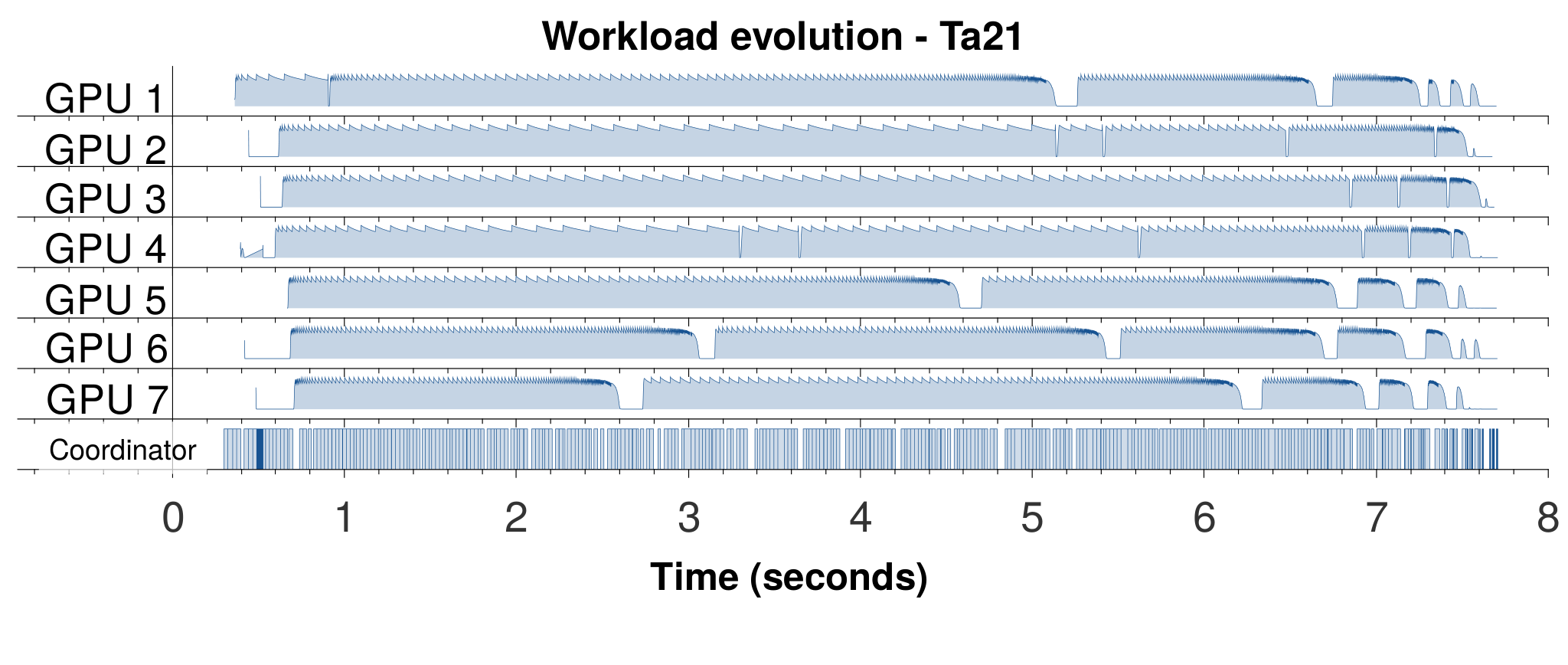

The small spikes in GPU-activity correspond to local work stealing operations, which are triggered when the ratio of active explorers decreases below . In turn, each of these operations triggers a worker-checkpoint. The fact that the frequency of these spikes varies throughout the exploration illustrates the irregularity of the search space. One can notice several sharp decreases of the activity level to zero, causing workers to remain idle until they receive new work units or the global termination signal. The response time of the coordinator is critical for the parallel efficiency of PBBCluster. One can also see that the relative worker idle time is much larger for the small Ta021 instance (8 seconds) than for Ta056 (15 minutes). Notably, although the solution of Ta056 lasts about 100 times longer than Ta021, the total number of global load balancing operations (idle workers acquiring new work) is approximately the same. Worker idle time occurs mainly in the initial work distribution phase (because the work-intensive parts of the search space are not yet detected) and in the final phase of the exploration (because overall available work is getting scarcer). These ramp-up and shut-down phases are limiting scalability for smaller instances, while they are negligible for large enough instances.
5.4 Scalability experiments on Jean Zay
| shorthand name | name | NN | (hh:mm) | NN/s | |
|---|---|---|---|---|---|
| small | 30_15_2 | 2317 | 122 G | 0:54 | 37.6 M |
| medium | 30_15_5 | 2421 | 564 G | 4:22 | 35.8 M |
| large | 30_15_9 | 2259 | 3660 G | 27:23 | 37.1 M |
In this subsection we experimentally evaluate the scalability of our approach on Jean Zay . To perform a meaningful scalability analysis, we need to choose problem instances which are small enough to be solved within a reasonable amount of time on a single device and large enough to justify the use of multiple GPUs (single-GPU execution time between hour and day). Moreover, the selected benchmark instances should be associated with different total workloads (tree sizes), but the granularity of the workload should be the same (i.e. the number of jobs and machines defining the instances should be identical). Taillard’s benchmark instances (except Ta056) are either too small or too large, so we selected instances 30_15_2, 30_15_5 and 30_15_9 from the VFR benchmark, defined by jobs and machines.
To avoid speedup anomalies, PBBCluster is initialized with the optimal solutions determined in preliminary runs. The sizes of explored critical trees (decomposed nodes) and corresponding single-GPU walltimes are shown in Figure 3. To simplify the presentation of results, we refer to these instances as small, medium and large. The critical tree of the small instance is composed of billion nodes and its exploration requires minutes of processing on a single V100, which corresponds to an average processing speed of nodes per second (NN/s). The large instance is times larger, requiring over hours of processing at approximately the same speed. For each of the three instances, runs are performed with quad-GPU nodes until the observed parallel efficiency drops below . Four MPI processes are mapped to each node and worker processes map to GPU devices via and the cudaSetDevice API function. As the master process occupies one slot on node , the corresponding number of GPUs is respectively .
For the three instances and an increasing number of GPUs, Figure 12(a) (on top) shows the elapsed walltime () with solid lines and the total active time of the coordinator () with dotted lines. The coordinator is considered “active” when it is not waiting on MPI_Probe, i.e. includes the time process spends receiving messages, converting intervals and processing worker requests. The linear scaling curve with respect to a single-GPU execution (no coordinator) is represented by black solid lines. However, as Figure 12(a) is drawn in -scale, deviations from the ideal linear case are hard to see. Therefore, Figure 12(b) (below) shows the corresponding parallel efficiency.
Parallel efficiency of at least is achieved with up to , , GPUs for the small, medium and large instances respectively; with , and , PBBCluster runs with efficiencies of , and respectively. For a larger number of GPUs the parallel efficiency drops off sharply, due to saturation of the coordinator process. Indeed, one can notice in Figure 12(a) that for , and GPUs, is close to , meaning that the coordinator is active nearly of the time and becomes a sequential bottleneck. However, with GPUs PBBCluster still reaches a speedup of for the large instance, reducing the execution time from over hours to about minutes. The results of this experiment indicate that for larger instances ( hours on a single device), PBBCluster can efficiently exploit this degree of parallelism, involving over 6 million independent tree exploration agents ( per GPU).
5.5 Comparison with previous solutions of instance Ta56
As mentioned in Section 1, the optimal makespan (3679) for the instance Ta056 is known since 2006. The solution was first obtained and proven optimal by a 25-day run of PBBGrid [18], exploiting on average CPUs. Over the last years, we have re-solved Ta056 several times on different platforms and with different sequential designs—but with the same initial condition, that is, initialized at 3680 (optimum-plus-one). For the purpose of comparing PBBCluster with existing large-scale parallel approaches, Table 4 shows a summary of those runs, indicating the used bounding/branching operator, the approximate number of explored nodes, computing platform and walltime, as well as an estimation of the corresponding energy consumption.
| Ref. | Year | LB/branching | tree size | Platform | walltime | kWh |
|---|---|---|---|---|---|---|
| [18] | 2006 | LB2/dyn(MinSum) | Avg. CPUs (max. 1195), Grid’5000/ULille | 25 d | 6000 | |
| [43] | 2015 | LB2/dyn(MinSum) | GTX980 (k Cuda cores), Univ. Mons | 9 d | 190 | |
| [43] | 2017 | LB2/dyn(MinSum) | P100 (k Cuda cores), Ouessant, IDRIS | 9 h | 110 | |
| [3] | 2020 | LB1/dyn(MinBranch) | E2630v3 (32 threads), Univ. Mons | 33 h | 5.6 | |
| 2020 | LB1/dyn(MinMin) | V100 (k Cuda cores), Jean Zay, IDRIS | 170s | 2 |
Using the same LB and branching rule as PBBGrid, Ta056 was solved in days on a single quad-GPU node (Maxwell) and in hours on a GPU-accelerated cluster of IBM “Minsky” nodes (2IBM Power8+ / 4P100). The improved sequential algorithm presented in [3] allows to re-solve Ta056 on a much smaller platform (-core CPU) in just hours, despite exploring a larger search tree. The PBBCluster approach presented in this work uses the same fine-grained LB (with a slightly different branching rule) and reduces the wallclock time to less than minutes on V100 GPUs.
Although we did not perform any exact measurements with wattmeters, an estimation of energy-consumption using TDP values provided by vendors shows the progress in terms of energy-consumption. About of the processor pool exploited by PBBGrid in 2006 are AMD Opteron dual-core CPUs and the remaining are mono-core Intel Pentium 4 or Celeron CPUs, mostly at nm feature size. The high-efficiency Opterons are listed at TDPs of about W and the Pentium 4 and Celerons are listed even higher. Assuming a TDP of W per core, we can estimate the total energy consumption of the PBBGrid resolution of Ta56 at . With the same lower bound and initial conditions, Ta56 was solved on the Ouessant prototype cluster in hours, using nodes (2 Power8 CPUs + 36 P100 GPUs). The energy consumption for this run can be estimated at . The same estimation for the improved LB1-based algorithm using nodes of Jean Zay gives . Compared to the first resolution of Ta56, the energy consumption has been reduced by three orders of magnitude.
5.6 Resolution of open PFSP instances
In this subsection, we give feedback on our attempts to solve instances from the Taillard benchmark for which optimal solutions are unknown. There are such instances in the -job/-machine class, in the group and in the group. For the sake of clarity in the following presentation of results, let us briefly recall the possible outcomes of a PBB execution:
- 1.
A solution with a better cost than the initial UB is found, but the algorithm does not terminate no proof of optimality, improved UB
- 2.
A solution with a better cost than the initial UB is found and the algorithm terminates proof of optimality and improved UB
- 3.
The algorithm terminates but the initial UB is not improved the optimal solution is larger or equal to the initial UB
- 4.
The algorithm does on terminate and the initial UB is not improved no information
50-job, 20-machine instances (Ta051-Ta060)
| —solved— | |||||||
| Instance | #GPUs | GPUh | NN | CPU-time | known UB | ||
| Ta058 | 256 | 13h17 | 3399 | 339T | 64 y | 3691 | 3691 |
| Ta053 | 128 | 7h59 | 1022 | 95T | 19 y | 3640 | 3640 |
| Ta052 | 384 | 1h54 | 729.6 | 68T | 14 y | 3704 | 3699 |
| Ta057 | 384 | 1h11 | 454.4 | 42T | 8.5 y | 3704 | 3704 |
| —remain open— | |||||||
| Best found | Comment | ||||||
| Ta051 | 3846 | equal to UB from [44] | |||||
| Ta054 | 3719 | equal to UB from [45], [46] | |||||
| Ta055 | 3610 | equal to UB from [47] | |||||
| Ta059 | 3741 | equal to UB from [45] | |||||
| Ta060 | 3755 | improved upper bound | |||||
Table 5 summarizes the execution statistics for the unsolved instances of the class— of them are solved to optimality for the first time. The results show that, even when optimal makespans for instances in this class are available, their optimality is very hard to prove. In all cases, the algorithm is initialized with the best-known solution from the literature. Taking for example Ta058, proving that no better solution than exists required over hours of processing on GPUs, performing node decompositions. Based on the CPU-GPU comparison shown in Figure 9, this corresponds to CPU-years of sequential processing. For instances Ta057 and Ta053, the best-known UB is also proven optimal, exploring search trees that are 240 (resp. 540) times larger than for Ta056.
In order to confirm the existence of a schedule with these optimal makespans, Ta057 is solved a second time, finding the same optimal solution when initialized at . For Ta058 and Ta053, additional explorations with the support of heuristic searches are performed until an optimal schedule is discovered. For Ta052, PBBCluster finds an improved schedule and proves its optimality in less than hours, using GPUs. Optimal permutations for these instances are given in A.
Instances Ta051, Ta054, Ta055, Ta59 and Ta060 remain open, despite using -k GPUh per instance in solution attempts. PBBCluster improves the initial UB provided for instance Ta060 by one unit to . For the remaining instances, PBBCluster is restarted with a larger initial UB and stopped when it finds the best-known UB. Enabling heuristic searches in PBBCluster, these solutions are found relatively quickly (usually within less than hour). The goal of these additional runs is to confirm the existence of best-known solutions reported in the literature. For the sake of completeness, corresponding permutation schedules are shown in A. Considering these observations, we can conjecture that the best-known UBs for the are optimal, but proofs of optimality are very hard to obtain.
100-job, 20-machine instances (Ta081-Ta090)
| —solved— | |||||||
| Instance | #GPUs | GPUh | NN | CPU-time | known UB | ||
| Ta083 | 64 | 0h24 | 25.8 | 2.2T | 290 d | 6271 | 6252 |
| Ta084 | 32 | 0h16 | 8.5 | 427G | 95 d | 6269 | 6254 |
| Ta090 | 128 | 78s | 3 | 168G | 31 d | 6434 | 6404 |
| —remain open— | |||||||
| old LB | new LB | LB | old UB | new UB | UB | ||
| Ta081 | 6106 | 6135 | +0.47% | 6202 | 6173 | -0.47% | |
| Ta085 | 6262 | 6270 | +0.13% | 6314 | 6286 | -0.44% | |
| Ta086 | 6302 | 6310 | +0.13% | 6364 | 6331 | -0.52% | |
| Ta087 | 6184 | 6210 | +0.42% | 6268 | 6224 | -0.70% | |
| Ta088 | 6315 | 6327 | +0.19% | 6401 | 6372 | -0.45% | |
| Ta089 | 6204 | 6224 | +0.32% | 6275 | 6247 | -0.44% | |
| Avg | +0.28% | -0.50% | |||||
For the 100-job instances Ta081-Ta090, prior to this work the exact solution was only known for Ta082. We add three instances to this list : Ta083, Ta084 and Ta090. Solution statistics and improved upper bounds are summarized in Table 6. After initial, inconclusive solution attempts—without using heuristic search threads—we try to tackle instances in this group in two ways:
- 1.
Using the best-known lower bound (as reported on E. Taillard’s website 66 6 http://mistic.heig-vd.ch/taillard/problemes.dir/ordonnancement.dir/flowshop.dir/best_lb_up.txt as initial UB, PBBCluster proves that no better solution exists, i.e. returns without discovering a better schedule. Then, the initial UB is incremented by and the search is restarted. Iterating over runs with an increasing initial UB, the best known lower bound is improved. This process is stopped when the algorithm finds and proves the optimality of a solution or when a fixed amount of time is elapsed.
- 2.
The exploration is initialized with the best-known UB and heuristic searches are used to discover better solutions.
The first approach leads to the resolution of Ta083, for which the previously best-known LB (6252) is optimal. Starting from one unit above the best-known LB (6253), an optimal schedule for Ta083 was found and proven optimal in minutes using GPUs. The explored search tree is composed of nodes, which is much smaller than the trees explored for the instances. Notably, once the optimal solution of Ta083 is found, the search terminates almost instantly—indeed, initialized with the optimum 6252, the exploration of the critical tree can be completed within a few seconds by a sequential PBB algorithm.
The second approach provides improved solutions for all remaining instances of this group. However, the exact PBB search alone is not able to find these solutions and best-found solutions strongly depend on the quality of the search heuristic. Optimality proofs are produced for two instances, Ta084 and Ta090, and in both cases the optimal makespan is equal to the best-known LB! The solution statistics shown in Table 6 correspond only to the run that resulted in the solution of the instance. For Ta084 and Ta090, several PBBCluster executions were performed prior to that final run (decreasing the initial upper bound and restarted from previous checkpoints)—unfortunately, exploration statistics were lost when restarting the algorithm from a global checkpoint.
The fact that the search completes relatively quickly (for the solved instances) suggests that some of the remaining instances of the class may be solved exactly, if heuristic searches are capable of finding an optimal solution. Indeed, contrary to the class, the hardness of the three solved instances stems from the difficulty of finding an optimal solution, while the optimality of the latter is relatively easy to prove.
For the six remaining instances, the exploration could not be completed within about -k GPUh of computation per instance. Although the required remaining time is by nature unpredictable, we used the total remaining work and LB-UB gaps as indicators for the hardness of an instance, and focused efforts on more reachable instances. For all unsolved instances, improved upper and lower bounds on the optimal makespan are reported in Table 6. One can see that for these instances, the previously best-known LB is not optimal (all best-known LBs are improved, on average by 0.32%). Taking for example Ta081, we have , which narrows down the previous LB-UB interval 6106—6202. On average, best-known UBs for the remaining instances are improved by . Permutation schedules for all improved UBs are provided in A.
It should be noted that for the class, ARPD values (with respect to best-known UBs) of best-performing metaheuristics reported in the literature are in the order of +0.5% [48, 46]. Our results show that, taking into account the improved UBs, actual optimality gaps of these methods are closer to +1.0%.
200-job, 20-machine instances (Ta101-Ta110)
| —solved— | |||||||
| Instance | #GPUs | GPUh | NN | CPU-time | known UB | ||
| Ta101 | 32 | 0h18 | 9.6 | 225G | 130 d | 11195 | 11158 |
| Ta107 | 32 | 0h06 | 3 | 41G | 41 d | 11360 | 11337 |
| Ta109 | 32 | 100s | 1 | 10G | 4 d | 11192 | 11146 |
| Ta108 | 32 | 28s | 1 | 2G | 80 h | 11334 | 11301 |
| —remain open— | |||||||
| old LB | new LB | LB | old UB | new UB | UB | ||
| Ta102 | 11143 | 11154 | +0.10% | 11203 | 11160 | -0.38% | |
In the class of Taillard’s benchmark, instances remain open, prior to this work. Four of them are solved exactly and the UB of the remaining instance is improved by 0.38%. All four solved instances are solved by running PBBCluster successively with increasing initial UBs. The exploration statistics shown in Table 7 correspond only to the last run which results in the instance’s solution. The largest of these instances, Ta101, is solved in minutes using 32 GPUs. Compared to the -job instances, most instances are “rather easy" to solve—although minutes on V100 GPU still correspond to an estimated computing time of 130 CPU-days). For two of the four solved instances the best-known LB is optimal (Ta107, Ta108). Instance Ta102 is much harder to solve. The range of possibly optimal makespan values was narrowed down to 11154–11160 (from 11143–11203), but multiple attempts consuming several thousands of GPU-hours were unsuccessful in further increasing (resp. decreasing) the lower (resp. upper) bound.
VFR instances
We also run PBBCluster on unsolved VFR instances [24], although less computing time per instance is spend on these attempts. We only attempt the resolution of instances with machines as the quality of LBs degrades too quickly with a higher number of machines. In A, optimality proofs and improved UBs are summarized. Overall, instances are solved exactly for the first time and improved best-known solutions are reported. Figure 13 summarizes, for each of the 48 instance classes, the number of remaining open instances and the number of optimal solutions provided in this paper. One can see that the unsolved instances with - machines are centered around -, which is consistent with the results obtained for Taillard’s benchmark.
6 Conclusions and future works
In this article, we have presented a hybrid Branch-and-Bound algorithm for exactly solving permutation-based combinatorial optimization problems on clusters composed of GPU-accelerated multi-core nodes (PBBCluster). The permutation flow-shop scheduling problem (PFSP) is used as a test-case. Our approach solves of Taillard’s benchmark instances to optimality for the first time, which is nearly half of the instances that remained open for years. Moreover, best-known upper bounds are improved for remaining instances. PBBCluster solves instance Ta056 in less than 3 minutes on the Jean Zay supercomputer, which is a four orders-of-magnitude improvement over the first exact solution in 2006, that required days of computation, using a grid-enabled algorithm exploiting CPUs on average.
This is not achieved through a one-shot research effort, nor by sheer brute-force computing power. In this paper we tried to give a synthetic overview of the key building blocks and successive contributions that have led to this breakthrough, while diving into details when the latter are critical. We have presented the design and implementation of PBBCluster, addressing challenging issues that occur at different levels, from low-level thread divergence to asynchronous inter-node communication and global checkpointing. Starting from the best available sequential design, we have proposed solutions for mapping a highly irregular and fine-grained tree-search algorithm to modern GPU-accelerated HPC clusters, exploiting all available sources of parallelism.
We have demonstrated the efficiency of the approach through computational experiments. Using a single V100 GPU, we observe speed-up factors up to compared to a single-threaded CPU-based implementation. The scalability of PBBCluster, using millions of GPU-based concurrent tree searches on up to 384 V100 GPUs (2 million CUDA cores) has been evaluated experimentally. An instance requiring 27 hours on a single GPU, is solved in 14 minutes on quad-GPU nodes, i.e. with 90% effiency. The largest instance tackled in this paper (Ta058) requires an equivalent computing power of 64 CPU-years—it is solved in hours, exploring a tree composed of nodes, which is more than the largest previously solved instance Ta056.
In the short term we plan to investigate the hybridization of exact PBB and approximate search methods, which has shown promising results. We will also investigate the use of high-productivity PGAS-based parallel computing environments, such as Chapel, that could greatly simplify the implementation of PBBCluster and parallel tree-search algorithms in general.
Acknowledgements
This work was granted access to the HPC resources of IDRIS under the allocation 2020-A0070611107 made by GENCI. Some of the experiments presented in this paper were carried out using the Grid’5000 testbed, supported by a scientific interest group hosted by Inria and including CNRS, RENATER and several Universities as well as other organizations (see https://www.grid5000.fr). Also, helpful advice by N. Melab, M. Mezmaz and D. Tuyttens on the presentation of this paper is gratefully acknowledged.
References
- Garey et al. [1976] M. R. Garey, D. S. Johnson, R. Sethi, The Complexity of Flowshop and Jobshop Scheduling, Mathematics of Operations Research 1 (1976) pp. 117–129.
- Taillard [1993] E. Taillard, Benchmarks for basic scheduling problems, European Journal of Operational Research 64 (1993) 278 – 285. URL: http://www.sciencedirect.com/science/article/pii/037722179390182M. doi:https://doi.org/10.1016/0377-2217(93)90182-M, project Management anf Scheduling.
- Gmys et al. [2020] J. Gmys, M. Mezmaz, N. Melab, D. Tuyttens, A computationally efficient branch-and-bound algorithm for the permutation flow-shop scheduling problem, European Journal of Operational Research 284 (2020) 814 – 833. URL: http://www.sciencedirect.com/science/article/pii/S037722172030076X. doi:https://doi.org/10.1016/j.ejor.2020.01.039.
- Asanovic et al. [2009] K. Asanovic, R. Bodik, J. Demmel, T. Keaveny, K. Keutzer, J. Kubiatowicz, N. Morgan, D. Patterson, K. Sen, J. Wawrzynek, D. Wessel, K. Yelick, A view of the parallel computing landscape, Commun. ACM 52 (2009) 56–67. URL: https://doi.org/10.1145/1562764.1562783. doi:10.1145/1562764.1562783.
- Bader et al. [2005] D. A. Bader, W. E. Hart, C. A. Phillips, Parallel algorithm design for branch and bound, in: Tutorials on Emerging Methodologies and Applications in Operations Research, Springer, 2005, pp. 5–1.
- Pruul et al. [1988] E. Pruul, G. Nemhauser, R. Rushmeier, Branch-and-bound and parallel computation: A historical note, Operations Research Letters 7 (1988) 65 – 69. URL: http://www.sciencedirect.com/science/article/pii/0167637788900673. doi:https://doi.org/10.1016/0167-6377(88)90067-3.
- Gendron and Crainic [1994] B. Gendron, T. G. Crainic, Parallel branch-and-bound algorithms: Survey and synthesis, Operations Research 42 (1994) 1042–1066. URL: http://www.jstor.org/stable/171985.
- Rao and Kumar [1987] V. N. Rao, V. Kumar, Parallel depth first search. part i. implementation, Int. J. Parallel Program. 16 (1987) 479–499. URL: https://doi.org/10.1007/BF01389000. doi:10.1007/BF01389000.
- Karypis and Kumar [1994] G. Karypis, V. Kumar, Unstructured tree search on simd parallel computers, IEEE Trans. Parallel Distributed Syst. 5 (1994) 1057–1072.
- Fonlupt et al. [1994] C. Fonlupt, P. Marquet, J.-L. Dekeyser, A data-parallel view of the load balancing experimental results on maspar mp-1, in: W. Gentzsch, U. Harms (Eds.), High-Performance Computing and Networking, Springer Berlin Heidelberg, Berlin, Heidelberg, 1994, pp. 338–343.
- Reinefeld and Schnecke [1994] A. Reinefeld, V. Schnecke, Work-load balancing in highly parallel depth-first search, in: Proceedings of IEEE Scalable High Performance Computing Conference, IEEE, 1994, pp. 773–780.
- Pessoa et al. [2016] T. C. Pessoa, J. Gmys, N. Melab, F. H. de Carvalho Junior, D. Tuyttens, A gpu-based backtracking algorithm for permutation combinatorial problems, in: J. Carretero, J. Garcia-Blas, R. K. Ko, P. Mueller, K. Nakano (Eds.), Algorithms and Architectures for Parallel Processing, Springer International Publishing, Cham, 2016, pp. 310–324.
- Rocki and Suda [2010] K. Rocki, R. Suda, Parallel minimax tree searching on gpu, in: R. Wyrzykowski, J. Dongarra, K. Karczewski, J. Wasniewski (Eds.), Parallel Processing and Applied Mathematics, Springer Berlin Heidelberg, Berlin, Heidelberg, 2010, pp. 449–456.
- Jenkins et al. [2011] J. Jenkins, I. Arkatkar, J. D. Owens, A. Choudhary, N. F. Samatova, Lessons learned from exploring the backtracking paradigm on the gpu, in: E. Jeannot, R. Namyst, J. Roman (Eds.), Euro-Par 2011 Parallel Processing, Springer Berlin Heidelberg, Berlin, Heidelberg, 2011, pp. 425–437.
- Crainic et al. [2006] T. G. Crainic, B. Le Cun, C. Roucairol, Parallel Branch-and-Bound Algorithms, John Wiley & Sons, Ltd, 2006, pp. 1–28. URL: https://onlinelibrary.wiley.com/doi/abs/10.1002/9780470053928.ch1. doi:https://doi.org/10.1002/9780470053928.ch1. arXiv:https://onlinelibrary.wiley.com/doi/pdf/10.1002/9780470053928.ch1.
- Anstreicher et al. [2002] K. Anstreicher, N. Brixius, J.-P. Goux, J. Linderoth, Solving large quadratic assignment problems on computational grids, Mathematical Programming 91 (2002) 563–588.
- Date and Nagi [2019] K. Date, R. Nagi, Level 2 reformulation linearization technique–based parallel algorithms for solving large quadratic assignment problems on graphics processing unit clusters, INFORMS Journal on Computing 31 (2019) 771–789. URL: https://doi.org/10.1287/ijoc.2018.0866. doi:10.1287/ijoc.2018.0866. arXiv:https://doi.org/10.1287/ijoc.2018.0866.
- Mezmaz et al. [2007] M. Mezmaz, N. Melab, E. Talbi, A grid-enabled branch and bound algorithm for solving challenging combinatorial optimization problems, in: 2007 IEEE International Parallel and Distributed Processing Symposium, 2007, pp. 1–9. doi:10.1109/IPDPS.2007.370217.
- Chakroun and Melab [2015] I. Chakroun, N. Melab, Towards a heterogeneous and adaptive parallel branch-and-bound algorithm, Journal of Computer and System Sciences 81 (2015) 72 – 84. URL: http://www.sciencedirect.com/science/article/pii/S0022000014000993. doi:https://doi.org/10.1016/j.jcss.2014.06.012.
- Vu and Derbel [2016] T.-T. Vu, B. Derbel, Parallel branch-and-bound in multi-core multi-cpu multi-gpu heterogeneous environments, Future Generation Computer Systems 56 (2016) 95 – 109. URL: http://www.sciencedirect.com/science/article/pii/S0167739X15003222. doi:https://doi.org/10.1016/j.future.2015.10.009.
- Gmys et al. [2017] J. Gmys, M. Mezmaz, N. Melab, D. Tuyttens, Ivm-based parallel branch-and-bound using hierarchical work stealing on multi-gpu systems, Concurrency and Computation: Practice and Experience 29 (2017) e4019. URL: https://onlinelibrary.wiley.com/doi/abs/10.1002/cpe.4019. doi:https://doi.org/10.1002/cpe.4019. arXiv:https://onlinelibrary.wiley.com/doi/pdf/10.1002/cpe.4019, e4019 cpe.4019.
- Lageweg et al. [1978] B. J. Lageweg, J. K. Lenstra, A. H. G. R. Kan, A General Bounding Scheme for the Permutation Flow-Shop Problem, Operations Research 26 (1978) 53–67. doi:10.1287/opre.26.1.53. arXiv:http://dx.doi.org/10.1287/opre.26.1.53.
- Ignall and Schrage [1965] E. Ignall, L. Schrage, Application of the branch and bound technique to some flow-shop scheduling problems, Oper. Res. 13 (1965) 400–412. URL: http://dx.doi.org/10.1287/opre.13.3.400. doi:10.1287/opre.13.3.400.
- Vallada et al. [2015] E. Vallada, R. Ruiz, J. M. Framinan, New hard benchmark for flowshop scheduling problems minimising makespan, European Journal of Operational Research 240 (2015) 666 – 677. URL: http://www.sciencedirect.com/science/article/pii/S0377221714005992. doi:https://doi.org/10.1016/j.ejor.2014.07.033.
- Mezmaz et al. [2014] M. Mezmaz, R. Leroy, N. Melab, D. Tuyttens, A multi-core parallel branch-and-bound algorithm using factorial number system, in: 2014 IEEE 28th International Parallel and Distributed Processing Symposium, 2014, pp. 1203–1212. doi:10.1109/IPDPS.2014.124.
- Gmys et al. [2016] J. Gmys, M. Mezmaz, N. Melab, D. Tuyttens, A gpu-based branch-and-bound algorithm using integer-vector-matrix data structure, Parallel Comput. 59 (2016) 119–139. URL: https://doi.org/10.1016/j.parco.2016.01.008. doi:10.1016/j.parco.2016.01.008.
- Bożejko [2009] W. Bożejko, Solving the flow shop problem by parallel programming, Journal of Parallel and Distributed Computing 69 (2009) 470 – 481. URL: http://www.sciencedirect.com/science/article/pii/S0743731509000215. doi:https://doi.org/10.1016/j.jpdc.2009.01.009.
- Melab et al. [2018] N. Melab, J. Gmys, M. Mezmaz, D. Tuyttens, Multi-core versus many-core computing for many-task branch-and-bound applied to big optimization problems, Future Generation Computer Systems 82 (2018) 472 – 481. URL: http://www.sciencedirect.com/science/article/pii/S0167739X16308706. doi:https://doi.org/10.1016/j.future.2016.12.039.
- de Bruin et al. [1995] A. de Bruin, G. A. P. Kindervater, H. W. J. M. Trienekens, Asynchronous parallel branch and bound and anomalies, in: A. Ferreira, J. Rolim (Eds.), Parallel Algorithms for Irregularly Structured Problems, Springer Berlin Heidelberg, Berlin, Heidelberg, 1995, pp. 363–377.
- Cappello [2009] F. Cappello, Fault tolerance in petascale/exascale systems: Current knowledge, challenges and research opportunities, The International Journal of High Performance Computing Applications 23 (2009) 212–226.
- Johnson [1954] S. M. Johnson, Optimal two- and three-stage production schedules with setup times included, Naval Research Logistics Quarterly 1 (1954) 61–68. doi:10.1002/nav.3800010110.
- Lomnicki [1965] Z. A. Lomnicki, A “branch-and-bound” algorithm for the exact solution of the three-machine scheduling problem, Journal of the Operational Research Society 16 (1965) 89–100. URL: https://doi.org/10.1057/jors.1965.7. doi:10.1057/jors.1965.7.
- Potts [1980] C. Potts, An adaptive branching rule for the permutation flow-shop problem, European Journal of Operational Research 5 (1980) 19 – 25. URL: http://www.sciencedirect.com/science/article/pii/0377221780900697. doi:https://doi.org/10.1016/0377-2217(80)90069-7.
- Knuth [1997] D. Knuth, The Art of Computer Programming, Volume 2: Seminumerical Algorithms, Reading, Ma (1997) 192. ISBN=9780201896848.
- Chakroun et al. [2013] I. Chakroun, N. Melab, M. Mezmaz, D. Tuyttens, Combining multi-core and gpu computing for solving combinatorial optimization problems, Journal of Parallel and Distributed Computing 73 (2013) 1563 – 1577. URL: http://www.sciencedirect.com/science/article/pii/S0743731513001615. doi:https://doi.org/10.1016/j.jpdc.2013.07.023, heterogeneity in Parallel and Distributed Computing.
- Carneiro et al. [2011] T. Carneiro, A. Muritiba, M. Negreiros, G. L. de Campos, A new parallel schema for branch-and-bound algorithms using gpgpu, in: Computer Architecture and High Performance Computing, Symposium on, IEEE Computer Society, Los Alamitos, CA, USA, 2011, pp. 41–47. URL: https://doi.ieeecomputersociety.org/10.1109/SBAC-PAD.2011.20. doi:10.1109/SBAC-PAD.2011.20.
- Vaidyanathan et al. [2015] K. Vaidyanathan, D. D. Kalamkar, K. Pamnany, J. R. Hammond, P. Balaji, D. Das, J. Park, B. Joó, Improving concurrency and asynchrony in multithreaded mpi applications using software offloading, in: SC ’15: Proceedings of the International Conference for High Performance Computing, Networking, Storage and Analysis, 2015, pp. 1–12. doi:10.1145/2807591.2807602.
- Hoefler and Lumsdaine [2008] T. Hoefler, A. Lumsdaine, Message progression in parallel computing - to thread or not to thread?, in: 2008 IEEE International Conference on Cluster Computing, 2008, pp. 213–222. doi:10.1109/CLUSTR.2008.4663774.
- Ruiz and Stützle [2007] R. Ruiz, T. Stützle, A simple and effective iterated greedy algorithm for the permutation flowshop scheduling problem, European Journal of Operational Research 177 (2007) 2033 – 2049. URL: http://www.sciencedirect.com/science/article/pii/S0377221705008507. doi:https://doi.org/10.1016/j.ejor.2005.12.009.
- Deroussi et al. [2010] L. Deroussi, M. Gourgand, S. Norre, Une adaptation efficace des mouvements de lin et kernighan pour le flow-shop de permutation, in: 8eme Conférence Internationale de MOdélisation et SIMulation: MOSIM, Tunisie, 2010. URL: http://citeseerx.ist.psu.edu/viewdoc/download?doi=10.1.1.167.2662&rep=rep1&type=pdf.
- Libralesso et al. [2020] L. Libralesso, P. A. Focke, A. Secardin, V. Jost, Iterative beam search algorithms for the permutation flowshop, 2020. URL: https://hal.archives-ouvertes.fr/hal-02937115, working paper or preprint.
- Choquette et al. [2018] J. Choquette, O. Giroux, D. Foley, Volta: Performance and programmability, IEEE Micro 38 (2018) 42–52. doi:10.1109/MM.2018.022071134.
- Gmys [2017] J. Gmys, Heterogeneous cluster computing for many-task exact optimization - Application to permutation problems, Ph.D. thesis, Université de Mons / Université de Lille, 2017. URL: https://hal.inria.fr/tel-01652000.
- Ravetti et al. [2012] M. G. Ravetti, C. Riveros, A. Mendes, M. G. Resende, P. M. Pardalos, Parallel hybrid heuristics for the permutation flow shop problem, Annals of Operations Research 199 (2012) 269–284.
- Pan et al. [2008] Q.-K. Pan, M. F. Tasgetiren, Y.-C. Liang, A discrete differential evolution algorithm for the permutation flowshop scheduling problem, Computers & Industrial Engineering 55 (2008) 795–816.
- Kizilay et al. [2019] D. Kizilay, M. F. Tasgetiren, Q.-K. Pan, L. Gao, A variable block insertion heuristic for solving permutation flow shop scheduling problem with makespan criterion, Algorithms 12 (2019) 100.
- Deroussi et al. [2006] L. Deroussi, M. Gourgand, S. Norre, New effective neighborhoods for the permutation flow shop problem, Technical Report LIMOS/RR-06-09, LIMOS, Université Clermont Auvergne, 2006. URL: https://hal.archives-ouvertes.fr/hal-00678053/.
- Dubois-Lacoste et al. [2017] J. Dubois-Lacoste, F. Pagnozzi, T. Stützle, An iterated greedy algorithm with optimization of partial solutions for the makespan permutation flowshop problem, Computers & Operations Research 81 (2017) 160 – 166. URL: http://www.sciencedirect.com/science/article/pii/S030505481630329X. doi:https://doi.org/10.1016/j.cor.2016.12.021.
Appendix A Solutions for benchmark instances
| Inst | old LB-UB 77 7 http://mistic.heig-vd.ch/taillard/problemes.dir/ordonnancement.dir/flowshop.dir/best_lb_up.txt and other sources. | best | Permutation schedule |
| Ta051 | 3771-3846 | 3846 | 20 31 39 27 43 15 44 11 8 45 35 37 6 17 34 28 7 14 42 33 40 24 5 29 10 2 18 47 48 21 46 1 16 49 12 23 22 36 32 38 19 9 26 25 13 41 30 4 50 3 |
| Ta052 | 3668-3704 | 3699 | 33 20 41 43 32 38 36 18 39 29 42 17 11 16 13 31 1 50 46 47 37 40 28 14 49 12 45 5 2 23 4 25 15 35 44 19 48 26 24 10 21 30 6 3 8 22 34 7 27 9 |
| Ta053 | 3591-3640 | 3640 | 24 4 10 28 21 8 37 46 16 22 31 5 39 2 32 11 25 49 47 20 15 48 26 3 35 17 14 43 27 45 9 1 19 50 30 6 36 34 29 42 23 33 41 12 7 18 40 44 13 38 |
| Ta054 | 3635-3719 | 3719 | 5 21 11 14 36 30 13 24 12 7 45 19 35 20 31 25 37 3 44 33 32 50 48 43 49 29 46 23 10 40 15 38 9 17 42 22 6 39 26 47 4 27 18 8 2 41 34 1 16 28 |
| Ta055 | 3553-3610 | 3610 | 40 48 4 2 19 31 50 28 20 49 34 5 23 21 32 25 43 45 44 18 26 36 33 42 27 16 41 14 8 47 39 38 10 6 22 17 30 12 13 3 37 9 7 1 46 24 15 29 35 11 |
| Ta056 | 3679 | 3679 | 14 37 3 18 8 50 5 42 33 40 4 45 17 27 20 21 13 49 43 11 10 41 24 15 16 19 44 32 26 28 46 1 36 39 47 25 30 7 2 31 23 6 48 22 29 34 9 35 38 12 |
| Ta057 | 3672-3704 | 3704 | 4 23 15 1 12 10 13 20 17 38 2 49 19 8 33 45 11 31 41 22 50 47 21 14 34 30 48 27 39 32 5 29 46 35 40 28 37 25 24 3 7 9 18 42 36 44 6 26 43 16 |
| Ta058 | 3627-3691 | 3691 | 39 32 18 7 4 20 29 31 6 8 48 19 33 12 27 30 38 26 15 36 47 21 35 10 2 17 41 5 9 28 3 25 16 1 24 37 49 42 45 22 11 50 40 46 13 43 14 44 34 23 |
| Ta059 | 3645-3741 | 3741 | 3 14 8 37 22 32 12 46 16 9 41 30 38 24 10 1 18 17 34 50 28 36 40 29 26 47 6 7 13 27 33 39 23 11 49 45 4 5 43 48 21 31 42 19 25 2 20 15 44 35 |
| Ta060 | 3696-3756 | 3755 | 33 12 19 8 3 22 15 23 2 9 40 1 11 21 36 32 25 47 31 16 37 10 42 18 50 27 29 13 44 14 38 34 17 28 39 6 26 49 46 5 24 41 20 30 35 7 48 45 43 4 |
| Inst | old LB-UB 88 8 http://mistic.heig-vd.ch/taillard/problemes.dir/ordonnancement.dir/flowshop.dir/best_lb_up.txt and other sources. | LB-UB | Permutation schedule |
| Ta081 | 6106-6202 | 6134-6173 | 54 78 59 74 79 1 83 89 31 3 51 50 80 99 61 25 9 35 76 40 82 70 12 85 5 16 91 81 6 60 56 33 22 10 44 100 63 65 21 96 28 55 62 86 94 18 24 30 53 20 2 45 47 48 23 27 4 11 41 92 29 88 46 73 64 71 36 57 93 32 67 98 90 77 37 87 42 26 66 39 95 52 68 58 72 84 34 38 43 69 19 15 14 75 17 97 8 49 13 7 |
| Ta082 | 6183 | 6183 | 50 49 95 65 32 27 87 66 80 52 69 90 35 82 72 89 19 31 10 40 14 96 62 79 78 2 33 59 75 93 48 77 13 71 9 70 54 22 1 36 5 7 34 84 91 46 68 100 61 98 53 20 47 76 92 58 43 15 45 99 26 23 55 42 73 38 11 4 85 37 86 97 74 8 41 51 3 63 64 60 83 30 24 25 56 16 88 67 28 17 6 44 18 21 12 94 29 81 39 57 |
| Ta083 | 6252-6271 | 6252 | 10 41 54 87 67 56 11 86 29 51 76 24 64 42 8 57 37 58 31 23 48 1 4 50 97 63 94 61 88 80 5 46 33 98 28 32 43 36 47 78 9 40 44 77 2 70 22 72 84 20 81 49 90 91 35 26 69 6 52 21 66 25 7 39 17 85 73 53 12 89 34 3 55 96 59 27 82 79 75 68 18 15 19 99 71 30 100 13 60 62 16 74 95 38 93 65 45 83 14 92 |
| Ta084 | 6254-6269 | 6254 | 74 98 45 44 25 79 38 57 58 23 67 89 43 29 90 51 88 60 84 50 69 65 1 15 5 71 92 46 95 26 56 96 52 8 7 91 16 55 86 77 22 78 54 87 64 63 76 32 41 68 11 99 13 59 72 3 47 28 37 70 30 93 31 62 85 6 4 9 73 2 61 81 39 17 20 35 34 19 94 100 24 42 83 21 10 75 82 66 27 18 12 49 97 48 14 40 53 33 80 36 |
| Ta085 | 6262-6314 | 6270-6285 | 64 10 98 51 50 97 12 32 16 56 14 11 72 30 38 61 70 74 33 85 76 58 62 1 53 69 41 28 37 3 57 52 95 15 17 39 90 88 94 65 18 2 20 9 46 87 60 71 5 8 45 89 6 4 23 31 21 92 40 86 22 93 82 36 26 63 25 99 55 80 44 66 29 34 35 49 68 59 42 54 81 13 27 96 7 77 48 100 75 78 84 24 91 83 79 73 43 19 47 67 |
| Ta086 | 6302-6364 | 6307-6331 | 83 32 2 12 21 33 39 92 37 69 1 86 31 82 88 89 56 72 38 25 80 76 71 9 65 55 7 34 10 66 94 23 75 52 58 26 8 99 63 40 60 100 98 81 95 68 48 97 16 45 77 17 20 91 84 6 5 14 62 3 87 35 15 28 57 30 79 46 4 67 13 64 24 36 85 78 27 50 54 74 93 41 70 44 18 53 22 49 11 51 73 19 43 61 29 59 47 96 42 90 |
| Ta087 | 6184-6268 | 6216-6223 | 93 85 62 96 95 67 94 32 49 73 27 88 60 19 20 53 16 23 64 84 14 51 98 39 45 48 89 57 33 28 59 12 78 13 42 29 43 69 22 90 31 34 91 8 55 36 61 21 77 17 41 52 79 80 65 3 82 71 24 47 11 38 50 72 40 58 100 97 99 9 4 7 66 46 6 54 87 18 10 56 30 70 81 15 63 37 25 5 2 1 92 26 74 35 44 83 68 86 76 75 |
| Ta088 | 6315-6401 | 6331-6385 | 39 62 29 90 31 87 36 22 71 5 78 72 45 81 12 24 69 55 1 91 70 58 14 44 56 67 93 10 25 7 9 52 83 37 57 41 77 73 96 59 23 28 100 35 88 27 17 94 49 51 18 75 66 86 64 4 50 19 74 6 3 98 60 68 40 80 95 53 48 89 30 47 65 85 46 76 54 33 42 34 82 11 16 63 79 84 8 43 32 38 21 13 2 99 61 92 26 15 97 20 |
| Ta089 | 6204-6275 | 6232-6247 | 88 15 2 74 60 43 77 17 42 89 95 68 47 90 21 24 62 50 96 81 94 4 41 80 19 16 54 20 39 82 12 97 38 30 46 63 79 10 23 78 61 65 40 55 58 26 84 37 59 70 73 11 25 86 92 34 32 18 7 53 76 71 27 87 48 33 14 56 69 83 100 31 6 8 13 85 93 51 72 57 3 99 45 52 1 9 36 67 44 66 75 28 64 35 29 49 22 5 91 98 |
| Ta090 | 6404-6434 | 6404 | 83 11 54 1 67 6 24 48 52 77 51 62 100 26 90 3 87 12 38 35 96 20 92 40 60 34 70 43 21 27 78 36 84 10 65 47 14 81 94 32 74 31 25 98 69 86 95 56 46 15 37 89 99 4 68 72 5 82 75 80 88 29 50 97 13 71 7 19 2 59 41 91 61 9 23 45 42 33 22 85 49 18 58 39 16 30 17 79 64 57 76 8 55 63 44 66 73 28 53 93 |
| Inst | old LB-UB | LB-UB | Permutation schedule |
| Ta101 | 11152-11195 | 11158 | 83 151 170 94 138 89 78 137 163 152 166 140 124 61 95 42 111 19 121 62 76 24 198 33 188 26 131 96 109 160 126 120 59 69 113 56 136 123 93 66 22 81 13 144 67 146 178 150 28 57 103 130 48 9 125 14 187 105 133 85 184 5 147 194 27 135 49 186 46 7 107 142 148 162 36 79 129 88 158 2 143 91 122 80 155 47 34 12 54 40 35 182 25 64 106 72 100 101 156 51 43 39 102 52 180 149 189 153 168 173 157 139 70 3 119 169 77 32 199 175 16 134 4 11 8 1 84 176 29 110 41 71 17 171 116 18 164 127 38 161 73 10 20 98 177 74 50 6 31 21 58 190 15 87 75 195 104 99 181 172 37 128 132 165 197 30 179 23 112 55 167 141 97 196 108 200 92 63 53 68 118 45 90 191 159 185 117 114 115 154 193 65 174 60 145 86 183 44 192 82 |
| Ta102 | 11143-11203 | 11152-11160 | 56 184 171 11 25 163 54 169 50 118 149 132 60 91 19 94 179 151 119 155 92 45 176 13 49 26 57 74 32 168 48 128 16 28 113 159 178 173 138 31 105 197 52 156 146 111 58 96 15 122 47 144 134 30 182 103 152 69 38 185 150 5 77 116 183 187 100 174 88 181 8 43 84 162 41 170 108 59 193 4 23 115 107 20 17 148 80 78 104 35 157 186 166 70 29 120 175 136 112 46 97 65 114 93 24 9 66 51 192 195 42 142 95 129 39 135 154 188 14 190 167 68 137 139 198 33 130 189 34 71 76 158 99 10 161 147 62 143 75 124 1 172 177 36 121 98 64 72 191 6 125 2 110 160 21 55 63 102 79 85 131 200 27 164 123 101 22 199 81 40 141 126 90 165 61 86 83 18 127 117 196 109 145 73 7 37 153 12 140 82 106 194 133 87 89 53 67 3 44 180 |
| Ta107 | 11337-11360 | 11337 | 168 200 190 66 175 10 44 109 65 161 23 141 102 193 182 27 125 166 68 140 28 9 59 3 99 83 165 89 57 159 90 163 149 171 111 117 18 154 25 194 98 131 87 64 136 4 196 138 169 164 75 19 91 80 129 181 62 45 124 137 110 74 100 17 47 50 156 184 143 70 84 56 37 78 14 32 142 35 72 86 77 105 42 112 157 151 167 123 67 20 33 95 144 51 76 63 183 8 114 85 24 128 6 82 46 153 39 31 88 93 61 81 145 54 162 197 52 107 172 139 58 133 38 118 158 189 94 134 185 179 7 101 150 21 191 180 177 11 135 127 178 60 148 96 195 115 69 119 30 147 73 15 49 1 48 55 130 132 13 176 40 53 113 121 41 92 188 198 5 34 71 170 79 104 186 36 106 174 155 152 16 97 160 26 146 126 187 12 43 22 122 173 29 103 2 199 116 108 192 120 |
| Ta108 | 11301-11334 | 11301 | 52 192 105 39 30 196 76 6 121 136 112 157 21 11 200 10 191 91 73 102 155 61 24 174 142 167 28 119 129 96 126 62 182 87 149 44 74 86 194 32 133 26 115 139 54 188 114 88 137 154 148 98 27 95 124 64 198 17 72 123 199 146 7 93 122 55 56 173 140 164 42 2 49 165 18 92 159 63 29 153 113 107 111 169 131 67 8 47 179 187 117 82 75 15 71 162 104 145 161 1 41 181 48 90 100 13 79 180 183 20 77 59 40 189 166 135 84 118 178 35 147 34 23 184 12 103 134 163 195 132 9 125 5 128 172 143 3 151 46 120 83 171 31 158 170 101 51 66 144 193 65 89 43 16 85 130 37 175 22 19 177 138 25 141 78 50 38 36 68 45 53 116 69 57 94 168 160 60 58 185 4 109 197 33 176 186 110 106 14 190 97 108 156 127 81 150 80 152 99 70 |
| Ta109 | 11145-11192 | 11146 | 55 10 166 190 32 199 19 23 25 101 108 77 106 72 111 37 170 176 57 4 91 6 21 100 70 29 123 16 17 79 121 41 198 27 103 47 194 120 74 69 186 113 38 61 196 175 116 68 181 76 177 126 185 86 136 28 83 197 132 3 112 167 75 154 54 139 169 163 12 60 153 80 157 9 109 89 133 39 155 178 141 88 191 43 44 125 59 53 137 31 81 118 149 48 143 7 127 182 97 193 33 62 35 49 90 52 200 195 184 104 102 188 95 46 187 159 66 15 42 140 147 65 128 5 183 13 85 63 26 11 179 2 129 156 115 142 34 24 144 161 192 165 22 172 45 73 189 162 131 150 107 138 105 8 180 171 51 18 119 87 96 146 78 99 82 36 114 67 56 164 98 122 14 93 134 64 94 1 152 110 160 151 168 158 174 84 173 50 71 145 30 130 40 124 148 20 117 58 92 135 |
| Instance | Instance | Instance | Instance | ||||
| 30_15_1 | 2378 | 40_15_1 | 3004 | 50_15_1 | 3305 | 60_15_1 | 3926 |
| 30_15_2 | 2317 | 40_15_2 | 2816 | 50_15_2 | 3342 | 60_15_2 | 3865 |
| 30_15_3 | 2304 | 40_15_3 | 2904 | 50_15_3 | 3292 | 60_15_3 | 3859 |
| 30_15_4 | 2444 | 40_15_4 | 2915 | 50_15_4 | 3510 | 60_15_4 | 3692 |
| 30_15_5 | 2421 | 40_15_5 | 2941 | 50_15_5 | 3332 | 60_15_5 | 3858 |
| 30_15_6 | 2306 | 40_15_6 | 2804 | 50_15_6 | 3341 | 60_15_6 | 3868 |
| 30_15_7 | 2316 | 40_15_7 | 2863 | 50_15_7 | 3475 | 60_15_7 | 3791 |
| 30_15_8 | 2366 | 40_15_8 | 2896 | 50_15_8 | 3420 | 60_15_8 | 3727 |
| 30_15_9 | 2259 | 40_15_9 | 2705 | 50_15_9 | 3194 | 60_15_9 | 3784 |
| 30_15_10 | 2385 | 40_15_10 | 2945 | 50_15_10 | 3394 | 60_15_10 | 3882 |
| 30_20_1 | 2643 | 40_20_1 | 3317 | 50_20_1 | 3683 | 60_20_1 | 4144 |
| 30_20_2 | 2835 | 40_20_2 | 3224 | 50_20_2 | 3704 | 60_20_2 | 4274 |
| 30_20_3 | 2783 | 40_20_3 | 3224 | 50_20_3 | 3773 | 60_20_3 | 4341 |
| 30_20_4 | 2680 | 40_20_4 | 3227 | 50_20_4 | 3702 | 60_20_4 | 4175 |
| 30_20_5 | 2672 | 40_20_5 | 3050 | 50_20_5 | 3622 | 60_20_5 | 4180 |
| 30_20_6 | 2715 | 40_20_6 | 3184 | 50_20_6 | 3779 | 60_20_6 | 4184 |
| 30_20_7 | 2712 | 40_20_7 | 50_20_7 | 3689 | 60_20_7 | 4251 | |
| 30_20_8 | 2812 | 40_20_8 | 3261 | 50_20_8 | 3775 | 60_20_8 | 4171 |
| 30_20_9 | 2795 | 40_20_9 | 3332 | 50_20_9 | 3799 | 60_20_9 | 4198 |
| 30_20_10 | 2805 | 40_20_10 | 3115 | 50_20_10 | 3756 | 60_20_10 | 4186 |
| Instance | Instance | Instance | Instance | ||||
| 100_20_1 | 6121 | 200_20_1 | 11181 | 300_20_1 | 15996 | 400_20_1 | 20952 |
| 100_20_2 | 6224 | 200_20_2 | 11254 | 300_20_2 | 16409 | 400_20_2 | 21346 |
| 100_20_3 | 6157 | 200_20_3 | 11233 | 300_20_3 | 16010 | 400_20_3 | 21379 |
| 100_20_4 | 6173 | 200_20_4 | 11090 | 300_20_4 | 16052 | 400_20_4 | 21125 |
| 100_20_5 | 6221 | 200_20_5 | 11076 | 300_20_5 | 21399 | 400_20_5 | 16245 |
| 100_20_5 | 6247 | 200_20_6 | 11208 | 300_20_6 | 16021 | 400_20_6 | 21075 |
| 100_20_7 | 6358 | 200_20_7 | 11266 | 300_20_7 | 16188 | 400_20_7 | 21507 |
| 100_20_8 | 6023 | 200_20_8 | 11041 | 300_20_8 | 16287 | 400_20_8 | 21198 |
| 100_20_9 | 6286 | 200_20_9 | 11008 | 300_20_9 | 16203 | 400_20_9 | 21236 |
| 100_20_10 | 6048 | 200_20_10 | 11193 | 300_20_10 | 16780 | 400_20_10 | 21456 |
| 600_20_5 | 31323 | 800_20_7 | 41342 |