Dispersion of neutrinos in a medium Preprint: KIAS-P20072

Coherent forward scattering of neutrinos propagating in background matter is shown to generate an effective (Wolfenstein) potential which modifies vacuum oscillations Wolfenstein:1977ue. In a medium of varying density, such an effect can lead to adiabatic neutrino conversion Mikheev:1986gs which is applied to solar neutrinos and confirmed by various experiments. This is in fact a particular feature of dispersion relation of fermions interacting with a medium of finite temperature and density Weldon:1982bn. Such a technique of quantum field theory at finite temperature has been used to reproduce the Wolfenstein potential Mannheim:1987ef; Pal:1989xs; Notzold:1987ik; Nieves:1989ez; DOlivo:1992lwg; Kiers:1997yt.

During the past decade, there was a great interest in considering various non-standard interactions of neutrinos in ordinary matter or dark matter (DM) to study their consequences in neutrino oscillations as well as cosmological and astrophysics observations Sawyer:1998ac; Farzan:2015hkd; Dev:2019anc; Venzor:2020ova; Berlin:2016woy; Brdar:2017kbt; Krnjaic:2017zlz; Liao:2018byh; Huang:2018cwo; Dev:2020kgz; Capozzi:2017auw; Capozzi:2018bps; Farzan:2018gtr; Smirnov:2019cae; Cline:2019seo. For a systematic study of medium effect, one needs to analyze dispersion relations modified by non-standard interactions through coherent forward scattering. Recently, such an analysis was performed considering various thermal and DM backgrounds Nieves:2018vxl; Ge:2019tdi; Choi:2019zxy; Babu:2019iml. In particular, the first attempt to derive a DM potential modifying neutrino oscillations was made in Ge:2019tdi; Choi:2019zxy. It was noticed that neutrino oscillations can occur solely by the medium effect even for massless neutrinos Choi:2019zxy.

The purpose of this article is to provide a systematic analysis of dispersion relation of neutrinos propagating in a medium. Specifically, we consider Weyl or Majorana, and Dirac neutrinos interacting with a complex scalar medium through a Yukawa coupling. The general equations of motion are highly non-linear and do not allow analytic solutions for the dispersion relation. However, they can be solved perturbatively considering various limits of physical interest with heavy mediator, heavy neutrino, high-momentum, and high density. Depending on the type of neutrinos, the effective mass and effective potential induced by the medium are different. From this analysis, one can see when the medium-induced oscillation occurs and how the asymmetric distribution of background field splits the energy spectrum of the neutrino and antineutrino. We also recognize the appearance of medium-induced mass-squared in the non-relativistic (or low-momentum) and high-density limit, which severely constrain the cosmological scenario of neutrino-DM interaction through CMB observations Aghanim:2018eyx. In the opposite limit of high-momentum, the astrophysical neutrino observations provide independent limits disfavoring a large part of parameter space Choi:2019ixb.

In Sec. II, we provide the general formula for the self-energy correction of the neutrino in a medium. In Sec. III, we find the approximate dispersion relation for each limiting case of Majorana and Dirac neutrinos. In Sec. IV, we consider the implications of the modified neutrino dispersions in a medium and conclude in Sec. V.

For neutrinos propagating in a medium, the equations of motion are modified due to the forward elastic scattering with the background field, which is expressed in terms of the self-energy correction. In general, the corrections are different for left-, and right-handed neutrinos as they may interact differently with the medium, and also for neutrinos and antineutrinos when the background distribution is CP asymmetric.

The left- and right-handed $u$ (or $v$) spinors in a medium satisfy the equations of motion

where $M_{\nu}$ is either Majorana or Dirac mass matrix and the self-energy correction $\not{\Sigma}$ takes the general form of

both for $u_{L}$ and $u_{R}$, or $v_{L}$ and $v_{R}$. Here $k_{\mu}$ is the four momentum of the background field and $\Sigma_{1,2}$ are functions of $p_{\mu},k_{\mu}$ and the medium density. The self-energy corrections of a particle and antiparticle are related by

that is, $\Sigma^{v}_{1}(p)=\Sigma^{u}_{1}(-p)$ and $\Sigma^{v}_{2}(p)=-\Sigma^{u}_{2}(-p)$, both for the left- and right-handed spinors. Thus the CP-violating effect appears through

showing that the asymmetric contributions of $\Sigma_{1}$ and $\Sigma_{2}$ are odd and even under the change of $p\to-p$.

For the Majorana neutrino, we have the relation:

and thus

So far, all the equations are applicable to the multi-flavor case for which it is non-trivial to solve the equations of motion. For a single flavor case with the mass $m_{\nu}$, the solutions of the equations of motion for neutrinos can be found when the determinant of the inverse propagator vanishes Weldon:1982bn:

with $L\equiv p-\Sigma_{L}$ and $R\equiv p-\Sigma_{R}$, which is applicable to both $u$ and $v$ spinors manifesting the standard relation: the negative energy solutions for the $u$ spinor correspond to the positive ones for the $v$ spinor.

In the rest frame of the medium, $k_{\mu}=m_{\phi}(1,\vec{0})$, Eq. (7) is factorized to $(L\cdot R-m_{\nu}^{2})^{2}=H^{2}$ allowing two types of solutions:

Here we defined $H\equiv L_{\bf p}R_{0}-R_{\bf p}L_{0}$ with $L\equiv(L_{0},\hat{\bf p}L_{\bf p})$ and $R\equiv(R_{0},\hat{\bf p}R_{\bf p})$ introducing the notation of $p=(E,\vec{\bf p})$ and $\hat{\bf p}=\vec{\bf p}/|\vec{\bf p}|$. More explicitly, we have

where ${\bf p}\equiv|\vec{\bf p}|$.

While it is impossible to find an analytic solution to the dispersion equation in general, it is useful to consider an approximate dispersion relation and illustrate some basic properties in a model-independent way. More complete solutions will be drawn in the next section considering various limits of a specific model.

When $|\Sigma_{1}|\ll 1$ and $m_{\phi}|\Sigma_{2}|\ll m_{\nu}$ or ${\bf p}$, it is straightforward to find the solution of Eq. (8) up to the first order in perturbation:

where we used the notation $\Sigma^{(0)}\equiv\Sigma(E_{0},\vec{{\bf p}})$ with $E_{0}\equiv\sqrt{{\bf p}^{2}+m^{2}_{\nu}}$. For a general fermion with four degrees of freedom, there appear four solutions of the dispersion relation. Two positive-energy solutions of Eq. (10) describe the dispersion relations of two neutrino states taking $\Sigma=\Sigma^{u}$, and two negative-energy solutions correspond to those of the anti-neutrino states which are obtained with $\Sigma=\Sigma^{v}$. In the limit ${\bf p}\to\infty$ (or $m_{\nu}\to 0$), the last term of Eq. (10) becomes $2m_{\phi}\Sigma_{2L}$ or $2m_{\phi}\Sigma_{2R}$ representing the dispersion of $\nu_{L}$ or $\nu_{R}$. In the opposite limit ${\bf p}\to 0$, both $\nu_{1}$ and $\nu_{2}$ receive the same correction as expected for the massive fermions at rest.

The dispersion relations in Eq. (9) or (10) can be adapted to the three types of neutrinos as follows.

i) Weyl neutrino ($m_{\nu}=0$):
For a massless neutrino, $\nu_{L}$ ($\nu_{R}$) is identified to $\nu$ ($\bar{\nu}$) and equivalently Eq. (9) is further decomposed into two seperate equations of motion

corresponding to the positive energy solutions of $L^{2}=0$ and $R^{2}=0$ with $\Sigma_{L}=\Sigma_{L}^{u}$ and $\Sigma_{R}=\Sigma_{R}^{u}$, respectively. Thus, we have the approximate solutions,

which correspond to $E_{\nu_{1},\nu_{2}}$ with $m_{\nu}=0$ in Eq. (10). In an asymmetric medium, Weyl neutrinos will receive asymmetric correction corresponding to the difference $\Sigma_{2L}-\Sigma_{2R}$.

ii) Majorana neutrino ($\nu=\nu^{c}$):
For a Majorana neutrino in the relativistic limit, we can identify $\nu_{L}$ ($\nu_{R}$) to $\nu$ ($\bar{\nu}$), and thus it is useful to take $u_{L}$ and $u_{R}$ as independent spinors using the relation Eq. (6) Choi:2019zxy. Then, applying Eq. (10), we get

where $\Sigma_{L,R}\equiv\Sigma^{u}_{L,R}$ used in Eq. (10). Note that $\Sigma_{L}\neq\Sigma_{R}$ in an asymmetric medium, and $\Sigma_{L}-\Sigma_{R}$ picks the asymmetric contribution. In a symmetric medium ( $L=R$), the neutrino and anti-neutrino have the same dispersion relation: $E_{\nu}=E_{\bar{\nu}}$ trivially from Eq. (9) or (13).

iii) Dirac neutrino ($\nu\neq\nu^{c}$ and $m_{\nu}\neq 0$):
The left- and right-handed components of a Dirac neutrino may interact differently with a medium leading to $\Sigma_{L}\neq\Sigma_{R}$. In the simple case of $\Sigma_{R}^{u,v}=0$, the relation Eq. (9) takes a much simpler form and Eq. (10) leads to

for the two neutrino states $\nu_{1,2}$ with $\Sigma_{L}=\Sigma_{L}^{u}$, and the corresponding negative-energy solutions give us $E_{\bar{\nu}_{1},\bar{\nu}_{2}}$ for the anti-neutrino states by replacing $\Sigma_{L}^{u}\to\Sigma_{L}^{v}$.

As a specific example, we consider a left-handed neutrino interacting with a background complex scalar $\phi$ and a fermion mediator $f$ through a Yukawa coupling $g$:

where $m_{f}$ is the Dirac mass.

The self-energy correction of the left-handed neutrino is calculated from the one-loop diagrams in Fig. 1:

where the bosonic and fermionic propagators in a finite density are given by

Here $f_{\phi}$ and $f_{f}$ are distribution functions of scalar and fermion in the medium. In this work, we assume that the medium is filled only by the complex scalar, that is, $f_{f}=0$ and

representing the number density of non-relativistic complex scalar in its rest frame:

where $n_{\phi}$ and $n_{\phi^{*}}$ are the number densities of particle and anti-particle in the background, respectively. The asymmetry of the complex scalar distribution is parameterized by $\epsilon$:

where $N_{\phi}=n_{\phi}+n_{\phi^{*}}\equiv\rho_{\phi}/m_{\phi}$.

Using the relation

with $E_{\phi}\equiv\sqrt{|\vec{k}|^{2}+m_{\phi}^{2}}=m_{\phi}$ in the non-relativistic limit, one obtains the self-energy corrections:

where $S(p)$ and $A(p)$ are the even and odd functions of $p$ given by

Here we defined

which is an effective mass-squared induced by the medium. Note that the above result is consistent with the diagramatic calculation Choi:2019zxy.

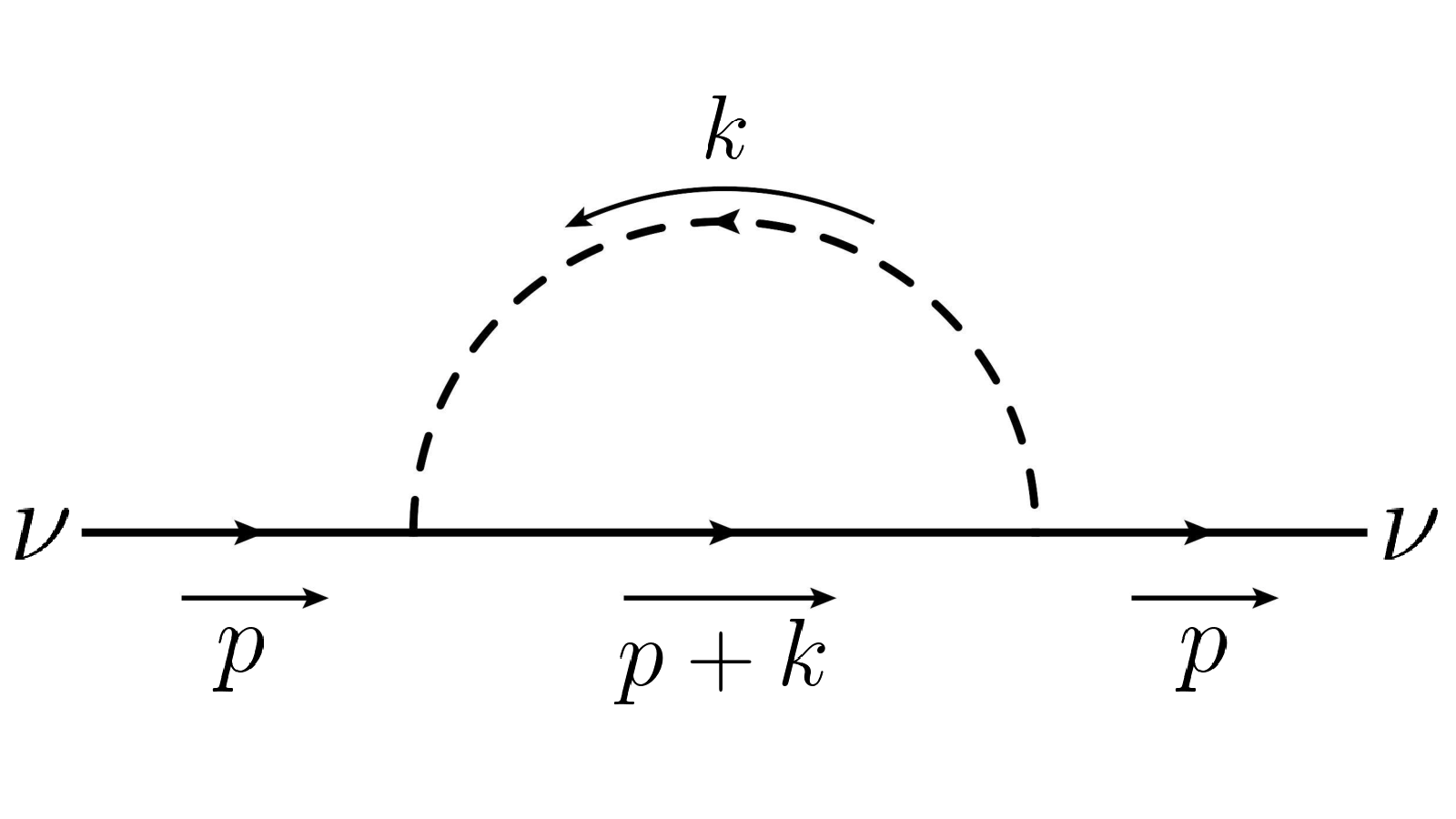We are now ready to discuss explicit dispersion relations considering various limits of different phenomenological interests. In each case, we perform perturbative expansion and find order-by-oder solutions for the dispersion relation.

In the approximate relation (10), the zeroth order expressions of $\Sigma^{(0)}$ can be written explicitly in terms of $S_{0}$ and $A_{0}$ defined by

with $E_{0}=\sqrt{{\bf p}^{2}+m_{\nu}^{2}}$. Then, the validity condition $|\Sigma_{1}^{(0)}|\ll 1$ requires $|S_{0}|$, $|\epsilon A_{0}|\ll 1$. Considering the medium of an ultra-light scalar field $\phi$, these quantities depend on the four energy scales: $\delta m^{2}_{\nu},m^{2}_{\nu},m_{f}^{2}$ and $2m_{\phi}{\bf p}$ ($m^{2}_{\phi}$ being the smallest). Then, the condition of $|S_{0}|\ll 1$, in particular, is realized in different physical situations when either of $m_{\nu}^{2},m_{f}^{2},2m_{\phi}{\bf p}$ dominates the others. In each case, we will use Eq. (10) or (13) to obtain the corresponding leading order correction.

To obtain more precise dispersion relations, one needs to perform order-by-order expansion from the original equation Eq. (7) and (8) and find the solutions in each order. This is also necessary for the situation when $\delta m^{2}_{\nu}$ is the largest as it gives us $\Sigma_{1}\simeq 1$.

One of the important consequences of the medium effect is the appearance of the neutrino oscillation term

in the ultra high-momentum limit. This implies that the observed neutrino oscillations can be due to the flavor mixing by the rest mass (Majorana or Dirac) and/or by the medium-induced “mass-squared” which does not involve chirality-flip or lepton-number violation. As a consequence, (massless) Weyl neutrinos can also oscillate in a medium Choi:2019zxy.

A natural candidate of such a medium is the ultra-light dark matter (DM) background which produces the effective neutrino mass-squared: $\delta m^{2}_{\nu}\propto\rho_{DM}/m^{2}_{DM}$. In this case, the DM density increases in the early universe and thus neutrinos undergo a high-density regime discussed in the previous section. At a redshift $z$, we have $\rho_{DM}(z)=\rho^{0}_{DM}(1+z)^{3}$ where $\rho^{0}_{DM}$ is the average DM density at present, and thus $\delta m^{2}_{\nu}$ becomes huge in the early Universe. Compared to the local DM density producing the observed neutrino mass-squared, $\delta m^{2}_{local}$, one has

where we used $\rho^{local}_{DM}=0.3\,{\rm GeV}/\,{\rm cm}^{3}$ and $\rho^{0}_{DM}=1.5\times 10^{-6}\,{\rm GeV}/\,{\rm cm}^{3}$. The energy density provided by the neutrinos during the decoupling time is constrained by the CMB measurement putting the upper bound on the neutrino mass $\sim 0.1$ eV Aghanim:2018eyx. This implies

which is too small to explain both the atmospheric and solar neutrino oscillations. Thus, the current density of DM interacting with neutrinos is required to be produced well after the decoupling time. To meet this unconventional demand, one could think of an early DM density consisting of another particles decaying very late to produce the neutrino-favorite DM background. Otherwise, it puts a strong limit on the effective neutrino mass induced by the current DM distribution.

At present, the scattering cross-section between neutrinos and DM is constrained by astrophysical neutrino observations from SN1987A and IceCube-170922A for the neutrino energy around $10\,{\rm MeV}$ and $300\,{\rm TeV}$, respectively Choi:2019ixb:

In our scenario with the Yukawa interaction Eq. (15), the scattering cross section between neutrino and dark matter at high energy is

and thus it requires

On the other hand, the effective neutrino mass-squared induced by the local DM distribution can describe the observed neutrino oscillations for

obtained from $\delta m^{2}_{\nu}=g^{2}\rho^{local}_{DM}/2m_{\phi}$ (22). Combing these two conditions, we get

The mediator mass is bounded from below $m_{\phi}<m_{f}$ for the stability of $\phi$, and the upper bound

is required for $2m_{\phi}E_{\nu}\gg m_{f}^{2}$.

In Fig. 2, we present the result of more precise calculation. The top panel shows the astrophysical bounds on $\sigma_{\nu-DM}/m_{\phi}$ as a function of the neutrino energy for $m_{\phi}=10^{-10}$eV, $m_{f}=0.1$eV, and $\epsilon=0$. The upper bounds on the Yukawa coupling are shown in blue and red depending on the types of neutrino-DM interactions. In the bottom panel, the green band shows the region of the DM mass and Yukawa coupling required by the atmospheric neutrino oscillation for the effective neutrino mass induced by the local DM distribution in order to solely resolve the current observations of neutrinos. The blue ($m_{f}=10^{-3}\,{\rm eV}$) and red ($m_{f}=0.1\,{\rm eV}$) solid lines represent the biggest coupling constant limited by the conditions: $m_{\phi}<m_{f}$ and $m_{\phi}>m^{2}_{f}/2E_{\nu}$ with $E_{\nu}=1$ GeV. The lower region of the line is allowed.

Dispersion relations of Weyl, Majorana and Dirac neutrinos propagating in a complex scalar medium are analyzed to study the medium effect in neutrino oscillations. Considering various limits of mass and energy scales in the model, we performed perturbative calculation to obtain the dispersion relation specific to each case. As a result, one can see how the medium effect modifies the neutrino oscillation term and contributes to the CP asymmetric correction. It is remarkable that the corrections to the mass-squared are different for Majorana and Dirac neutrinos in the high-density limit, and thus leading to different corrections to the neutrino oscillation terms.

Considering the medium of ultra-light scalar DM, one finds that neutrinos become “too heavy” in the early universe and thus the cosmological scenario for neutrino-DM interaction is highly restricted. On the other hand, the astrophysical neutrino observations put additional constraints on the model parameters in the high-momentum limit.