跳到论文正文
W Papers独立论文阅读器 arXiv:2012.09423 论文正文 计算阅读时间 · 0%
引用这篇论文根据当前论文元数据生成,正式投稿前建议核对。


License: arXiv.org perpetual non-exclusive license
arXiv:2012.09423v4 [cs.IT] 06 Dec 2022

Advanced NOMA Assisted Semi-Grant-Free Transmission Schemes for Randomly
Distributed Users

Huabing Lu,  Xianzhong Xie, 
Zhaoyuan Shi,  Hongjiang Lei, 
Helin Yang,  and Jun Cai
Thanks: H. Lu is with the Key Laboratory of Intelligent Control and Optimization for Industrial Equipment of Ministry of Education, Dalian University of Technology, Dalian 116024, China, and also with the School of Computer Science and Technology, Chongqing University of Posts and Telecommunications, Chongqing 400065, China (e-mail: luhuabing@dlut.edu.cn). Thanks: X. Xie is with the School of Computer Science and Technology, Chongqing University of Posts and Telecommunications, Chongqing 400065, China (e-mail: xiexzh@cqupt.edu.cn). Thanks: Z. Shi is with the Key Laboratory of Intelligent Perception and Computing of Anhui Province, Anqing Normal University, Anqing 246011, China (e-mail: shizy@stu.cqupt.edu.cn). Thanks: H. Lei is with the School of Communication and Information Engineering, Chongqing University of Posts and Telecommunications, Chongqing 400065, China (e-mail: leihj@cqupt.edu.cn). Thanks: H. Yang is with the Department of Information and Communication Engineering, School of Informatics, Xiamen University, Xiamen 361005, China (e-mail: helinyang066@xmu.edu.cn). Thanks: J. Cai is with the Network Intelligence and Innovation Lab (NI$ˆ2$L), Department of Electrical and Computer Engineering, Concordia University, Montreal, QC H3G 1M8, Canada (e-mail: jun.cai@concordia.ca).
Abstract

Non-orthogonal multiple access (NOMA) assisted semi-grant-free (SGF) transmission has recently received significant research attention due to its outstanding ability of serving grant-free (GF) users with grant-based (GB) users’ spectrum, which greatly improves the spectrum efficiency and effectively relieves the massive access problem of 5G and beyond networks. In this paper, we first study the outage performance of the greedy best user scheduling SGF scheme (BU-SGF) by considering the impacts of Rayleigh fading, path loss, and random user locations. In order to tackle the admission fairness problem of the BU-SGF scheme, we propose a fair SGF scheme by applying cumulative distribution function (CDF)-based scheduling (CS-SGF), in which the GF user with the best channel relative to its own statistics will be admitted. Moreover, by employing the theories of order statistics and stochastic geometry, the outage performances of both BU-SGF and CS-SGF schemes are analyzed. Theoretical results show that both schemes can achieve full diversity orders only when the served users’ data rate is capped, which severely limits the rate performance of SGF schemes. To further address this issue, we propose a distributed power control strategy to relax such data rate constraint, and derive analytical expressions of the two schemes’ outage performances under this strategy. Finally, simulation results validate the fairness performance of the proposed CS-SGF scheme, the effectiveness of the power control strategy, and the accuracy of the theoretical analyses.

Index Terms —NOMA, semi-grant-free, CDF-based scheduling, outage probability, fairness.

I Introduction

With the fast development of the Internet of Things (IoT), more and more devices are expected to be connected to the networks. It is predicted that the number of connected devices will reach 31.4 billion by 2023, and more than 60% of which will be IoT connections [2]. These large number of IoT devices arouse a paradigm shift from the current human-type communication oriented systems, where the packets are always quite long and transmitted based on grant-based (GB) protocols (namely, each communication device first transmits a scheduling request to the base station (BS) and then the BS sends a resource allocation grant back). On the contrary, short packets are common for the traffic generated by IoT devices [3, 4, 5], which is unsuitable to be transmitted with conventional GB protocols, since the lengthy request-grant process will be prohibitively costly for the signaling overhead and unacceptable as well for the resulting latency in delay-critical IoT applications [6, 7]. This motivates the development of Grant-free (GF) transmissions, where the request-grant process is omitted and some dedicated resource blocks are reserved for these IoT devices to transmit whenever the packets arrive [7, 9, 10, 8]. By applying GF schemes, the transmission delay resulting from the request-grant process is eliminated, and also the spectrum efficiency can be effectively improved. Nevertheless, without central access control of the BS, collisions may frequently occur in GF transmissions, since the spectrum reserved for GF transmission is ordinarily limited and it is inevitable that multiple users will choose the same resource in massive amount of IoT scenarios.

Integrating Non-orthogonal multiple access (NOMA) with GF transmission is a promising solution to this problem, by which multiple devices could transmit their signals using the same resource with different power levels or codebooks [11, 12, 13]. In this paper, we focus on power-domain NOMA [14, 15]. For comprehensive review of code-domain GF NOMA, we refer the readers to [16, 17, 18] and the references therein. The combination of power domain NOMA with random access (NOMA-RA) scheme for multichannel ALOHA was first discussed in [19], where users can choose the predetermined power levels for uplink transmission. Further, a layered random access scheme was proposed to enhance the throughput of multichannel ALOHA in [20]. By making use of channel inversion technique, the received power levels were set as two [21] and multiple [22] target values for NOMA-RA systems, and it is shown in [23] that increasing the number of power levels may further improve the throughput gain. Whereas, only successive interference cancellation (SIC) decoding strategy was considered in [19, 20, 21, 22, 23]. Based on slotted ALOHA (SA) and NOMA (SA-NOMA), [24] investigated the performance of both SIC and joint decoding (JD) strategies for wireless sensor networks, which showed that JD could effectively avoid outage error floors and SA-NOMA outperforms SA. However, in systems with a large quantity of devices, the number of connections may still exceed the NOMA capability for successful decoding, which deteriorates the system performance [13].

To alleviate this situation, NOMA assisted semi-grant-free (SGF) transmission schemes, which encourage GB users to share their resources with delay-tolerant IoT devices transmitting with GF protocols, have received much research attention [25, 13]. In SGF transmission schemes, some IoT devices with delay-tolerant packets can be bypassed with the resources which would otherwise be solely utilized by the GB users, so that both the connectivity and spectral efficiency can be improved. As the number of devices that content for the dedicated resources reserved for GF transmissions is reduced, the successful communication probability for the latency-critical IoT devices could be improved. Compared to pure GB transmission, lower signaling overhead is needed in SGF transmission, meanwhile the collision event is effectively managed compared with pure GF transmission [25].

I-A Related Work

The NOMA-assisted SGF transmission schemes have been investigated in [25, 26, 27, 28, 29, 30]. Specifically, the concept of SGF transmission was firstly proposed in [25], where two SGF mechanisms were developed to restrict the number of admitted GF users and ensure that the admission of the GF users does not cause too much performance degradation to the GB users. Based on the framework of [25], in order to improve the admitted GF users’ outage performances, Yang et al. [26] proposed an adaptive power allocation strategy to restrict the transmit power of the GB user, as the GB user’s signal was assumed to be always decoded at the second stage of SIC. Only Rayleigh fading was considered in [25, 26], while the impacts of path loss and user locations were not taken into account. In this regard, Jayanth et al. [27] considered a homogeneous user distribution scenario, and two GF users with the largest and second largest channel gains were admitted. To ensure the performance of the GB user, they exploited the principle of underlay cognitive radio to restrict the interference generated by the two admitted GF users within a threshold. Note that, the distances of all GF users to the BS are assumed to be the same in [27]. To step further, Zhang et al. investigated the spatial effect of random user locations on the performance of SGF schemes [28, 29]. They proposed a dynamic threshold protocol for the admission of the GF users and analyzed the outage performance [28] and ergodic rate [29] for the randomly scheduled GF users by employing stochastic geometry.

In the aforementioned studies [25, 26, 27, 28, 29], pre-fixed SIC decoding orders were assumed, which led to performance degradation for the GB user or outage error floors for the GB/GF users. To this end, Ding et al. [30] proposed a new SGF scheme by resorting to hybrid successive interference cancellation (HSIC) [31], in which the outage error floors could be effectively avoided if the product of the GB and GF users’ target signal-to-interference-plus-noise ratio (SINR) is less than 1, while the performance of the GB user could still be guaranteed as it solely occupies the channel. In other words, for the new SGF scheme, the admission of GF users can effectively improve the spectrum efficiency without affecting the GB user’s performance.

I-B Motivation and Contributions

Even though the aforementioned work has presented some innovative studies on NOMA-assisted SGF transmission schemes, three critical problems are still waiting for solution: 1) Only small scale fading (Rayleigh fading) was considered in [25, 26, 27, 30], and the impact of user locations was not taken into consideration. Although the impact of user locations was studied in [28] and [29], they failed to exploit multi-user diversity since random user scheduling was considered; 2) Most of the existing SGF schemes preferred to schedule the GF users with the strongest or weakest channel gains, in order to ensure the performance of the GB user [25] or maximize the rate performance of the scheduled GF users [25, 26, 27, 30]. This scheduling strategy may lead to the fairness11 1 In general, fairness in user scheduling can be divided into two categories [32]: throughput-based fairness and resource-based fairness. This paper focuses on resource-based fairness, namely, the GF users with different distances to the BS have an equal probability in scheduling. problem, since the users closer to the BS (cell boundary) may be scheduled more frequently due to smaller (larger) path loss. In practice, both sum rate and access fairness are critical system performance indicators in wireless networks [33, 34], especially for opportunistic scheduling [35]. Hence, it is necessary to develop an SGF scheme can ensure fair admission chance for the GF users with a reasonable rate performance guarantee; 3) In the new SGF scheme [30], robust transmission of the GF users (namely, the GF users can achieve non-zero diversity orders) can be achieved only in the case of capped target rate pairs. It is necessary to develop an SGF scheme can guarantee robust transmission in all cases.

Motivated by the previous discussions, this paper dedicates to investigating the SGF transmission schemes in a more practical scenario of considering the impact of spatial user locations. To be specific, we first extend the analysis on the outage performance of the SGF scheme with best user scheduling (BU-SGF) (namely, the GF user with the maximal data rate will be scheduled [30]) under a channel model consisting of Rayleigh fading, path loss, and random user locations by employing stochastic geometry. After that, to address the admission fairness issue inherent in the BU-SGF scheme, we introduce cumulative distribution function (CDF)-based scheduling to SGF scheme (termed as CS-SGF scheme), where the GF user whose channel condition is at its best state and most unlikely to be better will be admitted. Compared to the existing fair schemes, i.e., random selection SGF schemes [28, 29], the proposed CS-SGF scheme can effectively exploit multi-user diversity. Moreover, we develop a power control strategy, which can relieve the restrictions on the users’ target rates for achieving full diversity orders and further enhance the outage performance. The main contributions of this paper are outlined as follows:

∙\bullet We develop a tractable performance analysis framework for the BU-SGF scheme integrating Rayleigh fading, path loss, and spatial user locations. The proposed framework can be easily extended to analyze the performance of other fading channel models, such as Nakagami-mm fading, Rician fading, and so on.

∙\bullet We propose a fair admission scheme for SGF transmission systems by invoking CDF-based scheduling, which can effectively utilize multi-user diversity.

∙\bullet For both BU-SGF and CS-SGF schemes, we analyze the outage performances of the admitted GF users by applying order statistics and stochastic geometry. Meanwhile, we also derive the rate constraints under which both schemes can achieve full or zero diversity orders and identify the causes resulting in error floors.

∙\bullet We propose a distributed power control strategy for both GB and GF users to eliminate outage error floors and enhance the admitted GF users’ outage performance. We then re-evaluate the outage performances of BU-SGF and CS-SGF schemes with the proposed power control strategy and show insights on why the error floors can be avoided after applying the proposed power control strategy.

Our work extends the BU-SGF scheme [30] in the following several aspects: 1) Only Rayleigh fading is considered in [30], while our work takes both the path loss and the two-dimensional spatial locations of the users into consideration. Meanwhile, a more general outage performance analysis framework is proposed which can be adapted to other channel models with the impact of both path loss and spatial user locations; 2) The condition on the theoretical analysis in [30], i.e., the product of the two users’ target SINRs is less than 1, is removed to make our analysis more general; 3) The outage performance of the traditional BU-SGF scheme is re-evaluated by considering the power control strategy.

I-C Organization

The rest of this paper is organized as follows. Section II introduces the system model. Two SGF transmission schemes are presented in Section III. In Section IV, the outage performances of the two schemes with fixed transmit power are analyzed. Section V proposes the power control strategy and analyzes the outage performances of the two schemes after applying the power control strategy. In Section VI, simulation results are presented to verify the theoretical analyses and Section VII concludes this paper.

II System Model

In this section, the signal model is presented first, then the decoding scheme with HSIC and performance metric are introduced.
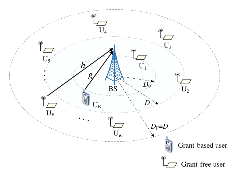
Refer to caption
Fig. 1: An illustration of the considered SGF system model.

II-A Signal Model

As shown in Fig. 1, a single-cell uplink cellular network is considered, where the BS is located at the center of the coverage disc area with radius DD. Similar to [25, 26, 30], we consider KK GF users (denoted as Uk, k∈{1,…,K}k\in\{1,\dots,K\}) and one GB user (denoted as UB\text{U}_{\text{B}}), where these GF users are distributed in the disc area 𝒟F\mathcal{D}_{\text{F}} with radius DFD_{\text{F}} (DF≤D)(D_{\text{F}}\leq D), and the GB user is randomly deployed in a ring region 𝒟B\mathcal{D}_{\text{B}} with inner radius D0D_{0} (D0≥0D_{0}\geq 0) and outer radius D1D_{1} (D1≤DD_{1}\leq D). The GF users are randomly distributed according to homogeneous Binomial point process (HBPP) [36], namely, the GF users are randomly deployed within the coverage area of the BS. The GB user communicates with the BS in conventional grant-based protocol and has been allocated one specific resource block. Thus, we assume that the channel state information (CSI) of the GB user is known to the BS [29]. Similar to [30], in each time slot, one GF user, denoted as UF{}_{\text{F}} (UF∈{U1,…,UK})(\text{U}_{\text{F}}\in\{\text{U}_{1},\dots,\text{U}_{K}\}), will be admitted for transmission using the resource block allocated to UB{}_{\text{B}} after distributed contention22 2 Distributed contention has been widely used in opportunistic carrier sensing[30, 40, 41], where the BS can schedule the most preferred user in a distributed manner. Take the strategy proposed in [41] as an example, which selects the user with the best channel condition to transmit. After estimating the CSI, each user selects a backoff time, e.g., πk\pi_{k} for the kk-th user, which decreases monotonously with increasing channel gain. Once the contention time window (with duration π0\pi_{0}) begins, the kk-th user will send a flag to the BS after πk\pi_{k} (πk<π0)(\pi_{k}<\pi_{0}) expires. Thus, the user with the best channel will send its flag first and hence be identified to the BS., where the contention criteria will be specified in Section III.

It is assumed that all nodes are equipped with a single antenna. We consider a composite channel model with both quasi-static Rayleigh fading and large scale path loss, and the channel coefficients are assumed to be invariant during each time slot and change independently between slots. At the beginning of each time slot, we assume that each user can estimate its CSI by exploiting pilot signals sent by the BS. The channel between the kk-th GF user Uk and the BS is modeled as hk=ζk1+rkαh_{k}=\frac{\zeta_{k}}{\sqrt{1+r_{k}^{\alpha}}}, where rkr_{k} represents the distance between Uk and the BS, α\alpha denotes the path loss exponent, and ζk\zeta_{k} represents Rayleigh fading coefficient with ζk∼𝒞​𝒩​(0,1)\zeta_{k}\sim\mathcal{CN}(0,1). Without loss of generality, we assume that the GF users’ channel gains are ordered as33 3 Note that, this assumption is used to facilitate performance analysis, and all nodes in the system do not know this order [30].

|h1|2≤⋯≤|hK|2.\displaystyle|h_{1}|^{2}\leq\dots\leq|h_{K}|^{2}. (1)

Similarly, the channel of UB{}_{\text{B}} to the BS is defined as g=ζB1+rBαg=\frac{\zeta_{\text{B}}}{\sqrt{1+r_{\text{B}}^{\alpha}}}, where ζB∼𝒞​𝒩​(0,1)\zeta_{\text{B}}\sim\mathcal{CN}(0,1) and rBr_{\text{B}} denotes the distance between UB{}_{\text{B}} and the BS.

Based on these assumptions, the CDFs of the unordered channel gains of the GF and GB users can be respectively expressed as [37, 38]

FF​(x)=\displaystyle F_{\text{F}}(x)= 2DF2​∫0DF[1−e−(1+rα)​x]​r​dr​≈(a)​12​∑l=1LΨl​(1−e−μl​x),\displaystyle\frac{2}{D_{\text{F}}^{2}}\int_{0}^{D_{\text{F}}}\left[1-e^{-(1+r^{\alpha})x}\right]rdr\overset{(a)}{\approx}\frac{1}{2}\sum_{l=1}^{L}\Psi_{l}\left(1-e^{-\mu_{l}x}\right), (2)
FB​(y)=\displaystyle F_{\text{B}}(y)= 2D12−D02​∫D0D1[1−e−(1+rα)​y]​r​dr​≈(b)​1D1+D0​∑n=1NΦn​(1−e−cn​y),\displaystyle\frac{2}{D_{1}^{2}-D_{0}^{2}}\int_{D_{0}}^{D_{1}}\left[1-e^{-(1+r^{\alpha})y}\right]rdr\overset{(b)}{\approx}\frac{1}{D_{1}+D_{0}}\sum_{n=1}^{N}\Phi_{n}\left(1-e^{-c_{n}y}\right), (3)

where ψl=cos​(2​l−12​L​π)\psi_{l}=\text{cos}\left(\frac{2l-1}{2L}\pi\right), μl=1+(DF2+DF2​ψl)α\mu_{l}=1+\left(\frac{D_{\text{F}}}{2}+\frac{D_{\text{F}}}{2}\psi_{l}\right)^{\alpha}, Ψl=πL​1−ψl2​(1+ψl)\Psi_{l}=\frac{\pi}{L}\sqrt{1-\psi_{l}^{2}}(1+\psi_{l}), φn=cos​(2​n−12​N​π)\varphi_{n}=\text{cos}\left(\frac{2n-1}{2N}\pi\right), ϕn=D1+D02+D1−D02​φn\phi_{n}=\frac{D_{1}+D_{0}}{2}+\frac{D_{1}-D_{0}}{2}\varphi_{n}, Φn=πN​1−φn2​ϕn\Phi_{n}=\frac{\pi}{N}\sqrt{1-\varphi_{n}^{2}}\phi_{n}, cn=1+ϕnαc_{n}=1+\phi_{n}^{\alpha}, LL and NN are parameters for ensuring complexity-accuracy trade-off. Due to the integrals in (2) and (3) can not be calculated in many communication scenarios (i.e., α>2\alpha>2) [37], the Gaussian-Chebyshev quadrature [39] is applied to perform approximation operations in (a)(a) and (b)(b). From (3), we can derive the probability density function (pdf) of UB{}_{\text{B}}’s channel gain as

fB​(y)≈1D1+D0​∑n=1NΦn​cn​e−cn​y.\displaystyle f_{\text{B}}(y)\approx\frac{1}{D_{1}+D_{0}}\sum_{n=1}^{N}\Phi_{n}c_{n}e^{-c_{n}y}. (4)

In each time slot, the BS will receive the superimposed signals transmitted from the GB user UB{}_{\text{B}} and the admitted GF user UF{}_{\text{F}}, which can be expressed as

y=h​PF​sF+g​PB​sB+n0,\displaystyle y=h\sqrt{P_{\text{F}}}s_{\text{F}}+g\sqrt{P_{\text{B}}}s_{\text{B}}+n_{0}, (5)

where sνs_{\nu} (ν∈{B,F}\nu\in\{\text{B},\text{F}\}) denotes the transmit symbol of Uν\text{U}_{\nu} with 𝔼⁡{|sν|2}=1\mathbb{E}\{|s_{\nu}|^{2}\}=1. PνP_{\nu} represents the transmit power of Uν\text{U}_{\nu}, hh (gg) denotes the channel from UF\text{U}_{\text{F}} (UB\text{U}_{\text{B}}) to the BS, and n0n_{0} represents the additive white Gaussian noise (AWGN) with zero mean and variance σ2\sigma^{2}. To facilitate the theoretical analysis, we assume that all the GF users have the same target data rate. Let RBR_{\text{B}} (RF)(R_{\text{F}}) and γB=2RB−1\gamma_{\text{B}}=2^{R_{\text{B}}}-1 (γF=2RF−1)(\gamma_{\text{F}}=2^{R_{\text{F}}}-1) respectively represent the target data rate and the target SINR of UB{}_{\text{B}} (UF\text{U}_{\text{F}}). Assuming the maximal transmit powers of the GB and GF users are the same and denoted as PmP_{m}. The notations used in this paper are summarized in Table I.

TABLE I: List of notations
Notation Description
KK Number of the GF users
𝒟F​(𝒟B)\mathcal{D}_{\text{F}}\ (\mathcal{D}_{\text{B}}) Disc (ring) region distributed with GF (GB) users
DD Coverage area of the BS
DFD_{\text{F}} Radius of the disc region 𝒟F\mathcal{D}_{\text{F}}
D0​(D1)D_{0}\ (D_{1}) Inner (outer) radius of the ring region 𝒟B\mathcal{D}_{\text{B}}
Uk\text{U}_{k} The kk-th GF user (k∈{1,…,K})(k\in\{1,\dots,K\})
UF\text{U}_{\text{F}} The admitted GF user (UF∈{U1,…,UK})(\text{U}_{\text{F}}\in\{\text{U}_{1},\dots,\text{U}_{K}\})
UB{}_{\text{B}} The GB user
α\alpha The path loss exponent
hkh_{k} Channel of Uk\text{U}_{k} with the BS
h⁡(g)h\ (g) Channel of UF\text{U}_{\text{F}} (UB{}_{\text{B}}) with the BS
rkr_{k} Distance between Uk\text{U}_{k} and the BS
rF​(rB)r_{\text{F}}\ (r_{\text{B}}) Distance between UF\text{U}_{\text{F}} (UB{}_{\text{B}}) and the BS
RF​(RB)R_{\text{F}}\ (R_{\text{B}}) Target rate of UF\text{U}_{\text{F}} (UB{}_{\text{B}})
γF​(γB)\gamma_{\text{F}}\ (\gamma_{\text{B}}) Target SINR of UF\text{U}_{\text{F}} (UB{}_{\text{B}}), γF=2RF−1\gamma_{\text{F}}=2^{R_{\text{F}}}-1 (γB=2RB−1)(\gamma_{\text{B}}=2^{R_{\text{B}}}-1)
σ2\sigma^{2} The noise power
PF​(PB)P_{\text{F}}\ (P_{\text{B}}) Transmit power of UF​(UB)\text{U}_{\text{F}}\ (\text{U}_{\text{B}})
ρF​(ρB)\rho_{\text{F}}\ (\rho_{\text{B}}) Transmit signal-to-noise ratio (SNR) of UF​(UB)\text{U}_{\text{F}}\ (\text{U}_{\text{B}}), ρF=PFσ2\rho_{\text{F}}=\frac{P_{\text{F}}}{\sigma^{2}}, ρB=PBσ2\rho_{\text{B}}=\frac{P_{\text{B}}}{\sigma^{2}}
Pm​(ρm)P_{m}\ (\rho_{m}) Maximal transmit power (SNR) of all users, ρm=Pmσ2\rho_{m}=\frac{P_{m}}{\sigma^{2}}
Pk​(ρk)P_{k}\ (\rho_{k}) Transmit power (SNR) of Uk\text{U}_{k}
αF​(αB)\alpha_{\text{F}}\ (\alpha_{\text{B}}) Target channel gain of UF\text{U}_{\text{F}} (UB{}_{\text{B}}), αF=γFρF\alpha_{\text{F}}=\frac{\gamma_{\text{F}}}{\rho_{\text{F}}}, αB=γBρB\alpha_{\text{B}}=\frac{\gamma_{\text{B}}}{\rho_{\text{B}}}
αF′​(αB′)\alpha^{\prime}_{\text{F}}\ (\alpha^{\prime}_{\text{B}}) Minimal target channel gain of UF\text{U}_{\text{F}} (UB{}_{\text{B}}), αF′=γFρm\alpha^{\prime}_{\text{F}}=\frac{\gamma_{\text{F}}}{\rho_{m}}, αB′=γBρm\alpha^{\prime}_{\text{B}}=\frac{\gamma_{\text{B}}}{\rho_{m}}
fX​(⋅)f_{X}(\cdot) Probability density function of XX
FX​(⋅)F_{X}(\cdot) Cumulative distribution function of XX
ℙ​{⋅}\mathbb{P}\{\cdot\} Probability of an event
≜\triangleq Be defined as
f⁡(a↦b)f(a\mapsto b) Replace aa in expression ff with bb
𝒞​𝒩​(μ,δ2)\mathcal{CN}(\mu,\delta^{2}) Complex Gaussian random variable with mean μ\mu and variance δ2\delta^{2}

II-B Decoding with HSIC

In NOMA transmission, SIC is applied at the receiver to decode both users’ signals, where one user’s signal is decoded and subtracted from the compound received signal first, and then another user’s signal is decoded. In fixed SIC (FSIC), the decoding order is pre-determined and is commonly employed in conventional SGF schemes [25, 26, 27, 28, 29]. However, FSIC may result in outage error floors, which leads to transmission robustness degradation of the GF users.

In order to effectively avoid outage error floors [31], HSIC is employed in this paper, where the decoding order is dynamically changed based on the instantaneous received SNR of UF\text{U}_{\text{F}}. Prior to user scheduling, the BS will first broadcast a threshold, denoted as τ0≜max​{0,τ⁡(|g|2)}\tau_{0}\triangleq\text{max}\left\{0,\tau(|g|^{2})\right\}, to all the GF users [30]. Here, τ⁡(|g|2)=αB−1​|g|2−1\tau(|g|^{2})=\alpha_{\text{B}}^{-1}|g|^{2}-1, which is derived based on the condition that the BS can successfully decode UB\text{U}_{\text{B}}’s signal at the first stage of SIC, namely, log​(1+ρB​|g|2τ⁡(|g|2)+1)≥RB\text{log}\left(1+\frac{\rho_{\text{B}}|g|^{2}}{\tau(|g|^{2})+1}\right)\geq R_{\text{B}}. Determing decoding order of HSIC can be divided into the following two cases:

  • •

    When the effective received SNR of UF\text{U}_{\text{F}}’s signal is larger than OPENτ0​(namely,​ρF​|h|2>τ0)\tau_{0}\ \text{(namely,}\ \rho_{\text{F}}|h|^{2}>\tau_{0}), the BS will decode UF\text{U}_{\text{F}}’s signal first with a data rate log​(1+ρF​|h|2ρB​|g|2+1)\text{log}\left(1+\frac{\rho_{\text{F}}|h|^{2}}{\rho_{\text{B}}|g|^{2}+1}\right). Otherwise, with the opposite decoding order, UB\text{U}_{\text{B}}’s signal cannot be successfully decoded, since ρF​|h|2>τ0\rho_{\text{F}}|h|^{2}>\tau_{0} leads to log​(1+ρB​|g|2ρF​|h|2+1)<RB\text{log}\left(1+\frac{\rho_{\text{B}}|g|^{2}}{\rho_{\text{F}}|h|^{2}+1}\right)<R_{\text{B}}, while UB\text{U}_{\text{B}}’s QoS should be satisfied with priority in SGF transmissions. Hence, UB\text{U}_{\text{B}}’s signal will be decoded at the second stage of SIC, with a data rate log​(1+ρB​|g|2)\text{log}\left(1+{\color[rgb]{0,0,0}\rho_{\text{B}}}|g|^{2}\right), which is the same as that achieved in OMA.

  • •

    When ρF​|h|2≤τ0\rho_{\text{F}}|h|^{2}\leq\tau_{0}, the BS will decode UB\text{U}_{\text{B}}’s signal first. Actually, in this case, for any decoding order, UB\text{U}_{\text{B}} can achieve the same performance as that in OMA transmission, and the BS can decode UB\text{U}_{\text{B}}’s signal at either the first or the second stage of SIC. Accordingly, UF\text{U}_{\text{F}} will achieve a data rate of log​(1+ρF​|h|2)\text{log}\left(1+\rho_{\text{F}}|h|^{2}\right) or log​(1+ρF​|h|2ρB​|g|2+1)\text{log}\left(1+\frac{\rho_{\text{F}}|h|^{2}}{\rho_{\text{B}}|g|^{2}+1}\right). Since log​(1+ρF​|h|2)>log​(1+ρF​|h|2ρB​|g|2+1)\text{log}\left(1+\rho_{\text{F}}|h|^{2}\right)>\text{log}\left(1+\frac{\rho_{\text{F}}|h|^{2}}{\rho_{\text{B}}|g|^{2}+1}\right), UB\text{U}_{\text{B}}’s signal will be decoded first to maximize UF\text{U}_{\text{F}}’s data rate.

II-C Performance Metric

In this paper, we use outage probability as a performance metric for different SGF schemes, which represents the probability that the instantaneous achievable rate of an admitted GF user is less than a target rate. To gain more insights, diversity order will also be derived. The diversity order highlights the asymptotic scaling law of the outage probability to the transmit SNR, which is defined as [42]

d=−limρ→∞​log​𝒫​(ρ)log​ρ,\displaystyle d=-\underset{\rho\rightarrow\infty}{\text{lim}}\frac{\text{log}\mathcal{P}(\rho)}{\text{log}\rho}, (6)

where 𝒫⁡(ρ)\mathcal{P}(\rho) and ρ\rho denote the outage probability and transmit SNR, respectively.

We would like the diversity order to be non-zero, which indicates that the outage probability will constantly decrease with the increase of the transmit SNR. Intuitively, we would also like the diversity order to be as large as possible, which means the outage probability will decrease fast with the increase of transmit SNR. However, when ρ→∞\rho\rightarrow\infty, if the outage probability is a constant and is independent of the transmit SNR, an outage error floor occurs, which may lead to a degradation of transmission robustness.

III SGF schemes

In this section, we first introduce the BU-SGF scheme [30] with randomly deployed users, then the proposed fair CS-SGF scheme is presented.

III-A BU-SGF Scheme

In BU-SGF scheme, the GF user which can achieve the maximal data rate will be admitted to access UB{}_{\text{B}}’s channel. It can effectively utilize multi-user diversity and avoid the outage error floor of the admitted GF user, while guaranteeing the GB user’s performance to be the same as it solely occupies the channel [30]. However, only the Rayleigh fading channel was taken into consideration in [30] and the analytical results can not be easily extended to other channel models. In reality, the users are always randomly distributed and their channels are also impacted by the path loss, therefore, it is necessary to consider these two factors in performance analysis. Instead, we extend the traditional BU-SGF scheme, where the admission procedure consists of the following six steps:

  1. 1.

    The BS sends pilot signals.

  2. 2.

    Each user estimates its own CSI.

  3. 3.

    UB\text{U}_{\text{B}} feedbacks its transmit SNR ρB\rho_{\text{B}}, target rate RBR_{\text{B}}, and CSI gg to the BS.

  4. 4.

    The BS calculates UB\text{U}_{\text{B}}’s decoding threshold τ0\tau_{0}, and broadcasts UB\text{U}_{\text{B}}’s effective received SNR ρB​|g|2\rho_{\text{B}}|g|^{2} and τ0\tau_{0} to all GF users.

  5. 5.

    Uk\text{U}_{k} calculates its transmit data rate (if admitted), which is log​(1+ρk​|hk|2ρB​|g|2+1)\text{log}\left(1+\frac{\rho_{k}|h_{k}|^{2}}{\rho_{\text{B}}|g|^{2}+1}\right) if ρk​|hk|2>τ0\rho_{k}|h_{k}|^{2}>\tau_{0}, or log​(1+ρk​|hk|2)\text{log}\left(1+\rho_{k}|h_{k}|^{2}\right) if ρk​|hk|2≤τ0\rho_{k}|h_{k}|^{2}\leq\tau_{0}, where ρk​|hk|2\rho_{k}|h_{k}|^{2} denotes Uk\text{U}_{k}’s effective received SNR (if admitted). Note that, HSIC is applied here.

  6. 6.

    The GF user with the maximal data rate will be admitted to transmit through distributed contention. Thus, the contention criterion is each GF user’s achievable data rate.

In BU-SGF scheme, the achievable rate of Uk\text{U}_{k}, log​(1+ρk​|hk|2ρB​|g|2+1)\text{log}\left(1+\frac{\rho_{k}|h_{k}|^{2}}{\rho_{\text{B}}|g|^{2}+1}\right) or log​(1+ρk​|hk|2)\text{log}\left(1+\rho_{k}|h_{k}|^{2}\right), is an increasing function with respect to the channel gain |hk|2|h_{k}|^{2}. By considering randomly distributed GF users with different distances to the BS, the GF users closer to the BS can achieve higher data rate due to smaller path loss. Since the BU-SGF scheme always admits the GF user with the largest data rate, the GF users closer to the BS will be scheduled more often. On the contrary, the GF users far from the BS will be scheduled seldomly and their generated data may become overflow, which results in severe fairness issue. In the next subsection, we will propose a fair SGF scheme, which can schedule each GF user with equal probability.

III-B CS-SGF Scheme

We handle the fairness issue of SGF scheme by resorting to CDF-based scheduling, where the GF user with the largest CDF value about its channel gain, namely, the GF user whose channel is good enough relative to its own statistics, will be admitted [43]. Since all the GF users’ channels are independent with each other and their channel gains’ CDF values are uniformly distributed in [0, 1] [32], each GF user will have the same probability to obtain the largest CDF value and then the admission fairness can be guaranteed. Assume that the CDF of Uk\text{U}_{k}’s channel gain |hk|2|h_{k}|^{2} is denoted as Fk​(x)F_{k}(x)44 4 In this paper, we use “CDF” to denote the cumulative distribution function, e.g., Fk​(x)F_{k}(x), and use “CDF value” to represent the corresponding output value of a CDF with a specific input xx.. For Rayleigh small-scale fading, the CDF of Uk\text{U}_{k}’s channel gain with a given distance rkr_{k} (the distance from Uk\text{U}_{k} to the BS) can be expressed as

Fk​(x|rk)=1−e−(1+rkα)​x.F_{k}(x|r_{k})=1-e^{-(1+r_{k}^{\alpha})x}. (7)

We assume that the BS sends pilot signals at the beginning of each time slot for synchronizing uplink transmissions. In time division duplexing (TDD) mode, each GF user can estimate its channel gains by measuring these pilot signals [19]. By applying non-parametric CDF based scheduling (NPCS) or parametric CDF based scheduling (PCS) [44], each GF user can estimate its CDF based on the estimation of channel gains [32]. When a GF user wants to transmit data at a specific time slot, it will estimate the instantaneous channel gain at the beginning of that time slot, and then obtain the corresponding CDF value by substituting the estimated result into the CDF. By using distributed contention control strategy [41], the GF user with the largest CDF value can be admitted. The contention criterion is each GF user’s CDF value, namely, each GF user’s backoff time is set to be inversely proportional to its CDF value. The admission procedure of CS-SGF scheme can be outlined as follows:

  1. 1.

    The BS sends pilot signals.

  2. 2.

    Each user estimates its own CSI (Based on that, each user can estimate its CDF after a long-term observation of the CSI.).

  3. 3.

    UB\text{U}_{\text{B}} feedbacks its transmit SNR ρB\rho_{\text{B}}, target rate RBR_{\text{B}}, and CSI gg to the BS.

  4. 4.

    The BS calculates UB\text{U}_{\text{B}}’s decoding threshold τ0\tau_{0}, and broadcasts UB\text{U}_{\text{B}}’s effective received SNR ρB​|g|2\rho_{\text{B}}|g|^{2} and τ0\tau_{0} to all GF users.

  5. 5.

    The GF user with the maximal CDF value will be admitted to transmit through distributed contention, and the contention criterion is each GF user’s CDF value.

  6. 6.

    The admitted GF user, UF{}_{\text{F}}, calculates its transmit data rate, which is log​(1+ρF​|hF|2ρB​|g|2+1)\text{log}\left(1+\frac{\rho_{\text{F}}|h_{\text{F}}|^{2}}{\rho_{\text{B}}|g|^{2}+1}\right) if ρF​|hF|2>τ0\rho_{\text{F}}|h_{\text{F}}|^{2}>\tau_{0}, or log​(1+ρF​|hF|2)\text{log}\left(1+\rho_{\text{F}}|h_{\text{F}}|^{2}\right) if ρF​|hF|2≤τ0\rho_{\text{F}}|h_{\text{F}}|^{2}\leq\tau_{0}. HSIC is applied here.

IV Performance Analysis for SGF Schemes with Fixed Transmit Power

In this section, the outage probabilities and achieved diversity orders of UF\text{U}_{\text{F}} are analyzed for both BU-SGF and CS-SGF schemes. Note that, since UB{}_{\text{B}} can always achieve the same performance as that in OMA for both schemes, we only characterize UF\text{U}_{\text{F}}’s outage performance [30]. The main steps of the analysis procedure are listed as follows:

  1. 1.

    Derive UF\text{U}_{\text{F}}’s outage probability expressions.

  2. 2.

    Convert, combine, and/or simplify the outage probability expressions for easier calculation.

  3. 3.

    Calculate the approximation expressions for the outage probabilities by using the CDF/pdf expressions of the users’ channel gains.

  4. 4.

    Derive the high SNR approximations of the outage probabilities and the achieved diversity orders.

For ease of theoretical analysis, the GF users are assumed to use a same fixed transmit SNR ρF\rho_{\text{F}} in both BU-SGF and CS-SGF schemes, namely, ρk=ρF​for​k∈{1,…,K}\rho_{k}=\rho_{\text{F}}\ \text{for}\ k\in\{1,\dots,K\}.

IV-A Performance Analysis for BU-SGF Scheme

According to the previous description, the outage probability of UF\text{U}_{\text{F}} for BU-SGF scheme can be denoted as

𝒫BU=\displaystyle\mathcal{P}_{\text{BU}}= ∑k=0Kℙ{Ek,max{log(1+ρF|hi|2),1≤i≤k}<RF,\displaystyle\sum_{k=0}^{K}\mathbb{P}\left\{E_{k},\text{max}\{\text{log}(1+\rho_{\text{F}}|h_{i}|^{2}),1\leq i\leq k\}<R_{\text{F}},\right. (8)
max{log(1+ρF​|hi|2ρB​|g|2+1),k<i≤K}<RF},\displaystyle\text{max}\{\text{log}(1+\frac{\rho_{\text{F}}|h_{i}|^{2}}{\rho_{\text{B}}|g|^{2}+1}),k<i\leq K\}<R_{\text{F}}\},

where EkE_{k} denotes the event that there are kk users’ effective received SNRs are less than UB\text{U}_{\text{B}}’s decoding threshold τ0\tau_{0}.

As the GF users transmit with fixed SNR ρF\rho_{\text{F}} and their channel gains are ordered as (1), the outage probability can be rewritten as

𝒫BU=\displaystyle\mathcal{P}_{\text{BU}}= ℙ⁡{E0,RKfs<RF}+ℙ⁡{EK,RKss<RF}+∑k=1K−1ℙ⁡{Ek,Rkss<RF,RKfs<RF},\displaystyle\mathbb{P}\left\{E_{0},R_{K}^{\text{fs}}<R_{\text{F}}\right\}+\mathbb{P}\left\{E_{K},R_{K}^{\text{ss}}<R_{\text{F}}\right\}+\sum_{k=1}^{K-1}\mathbb{P}\left\{E_{k},R_{k}^{\text{ss}}<R_{\text{F}},R_{K}^{\text{fs}}<R_{\text{F}}\right\}, (9)

where Rkfs≜log​(1+ρF​|hk|2ρB​|g|2+1)R_{k}^{\text{fs}}\triangleq\text{log}(1+\frac{\rho_{\text{F}}|h_{k}|^{2}}{\rho_{\text{B}}|g|^{2}+1}) and Rkss≜log​(1+ρF​|hk|2)R_{k}^{\text{ss}}\triangleq\text{log}(1+\rho_{\text{F}}|h_{k}|^{2}) represent the kk-th (k∈{1,…,K}k\in\{1,\dots,K\}) GF user’s achievable rates when its signal is decoded at the first and second stages of SIC, respectively. The superscripts “fs” and “ss” refer to the first and second stages of SIC, respectively. In (9), the first term shows the outage probability of the admitted GF user (namely, the KK-th user whose signal is decoded at the first stage of SIC) when all GF users’ effective received SNRs are larger than UB\text{U}_{\text{B}}’s decoding threshold τ0\tau_{0}; the second term computes the outage probability of the admitted GF user (the KK-th user whose signal is decoded at the second stage of SIC) when all the users’ effective received SNRs are lower than τ0\tau_{0}; and the third term considers the cases when there are k⁡(1≤k≤K−1)k\ (1\leq k\leq K-1) users with effective received SNRs lower than τ0\tau_{0}, the probability of the admitted GF user (either the kk-th user whose signal is decoded at the second stage of SIC, or the KK-th user whose signal is decoded at the first stage of SIC) is in outage.

Note that, in the case of |g|2<αB=γBρB|g|^{2}<\alpha_{\text{B}}=\frac{\gamma_{\text{B}}}{\rho_{\text{B}}}, the decoding threshold τ0≜max​{0,αB−1​|g|2−1}=0\tau_{0}\triangleq\text{max}\left\{0,\alpha_{\text{B}}^{-1}|g|^{2}-1\right\}=0. Then the outage probability can be expressed as

𝒫BU=\displaystyle\mathcal{P}_{\text{BU}}= ℙ⁡{|g|2>αB,E0,RKfs<RF}⏟T0+∑k=1K−1ℙ⁡{|g|2>αB,Ek,Rkss<RF,RKfs<RF}⏟Tk\displaystyle\underbrace{\mathbb{P}\left\{|g|^{2}>\alpha_{\text{B}},E_{0},R_{K}^{\text{fs}}<R_{\text{F}}\right\}}_{T_{0}}+\sum_{k=1}^{K-1}\underbrace{\mathbb{P}\left\{|g|^{2}>\alpha_{\text{B}},E_{k},R_{k}^{\text{ss}}<R_{\text{F}},R_{K}^{\text{fs}}<R_{\text{F}}\right\}}_{T_{k}} (10)
+ℙ⁡{|g|2>αB,EK,RKss<RF}⏟TK+ℙ⁡{|g|2<αB,RKfs<RF}⏟TK+1,\displaystyle+\underbrace{\mathbb{P}\left\{|g|^{2}>\alpha_{\text{B}},E_{K},R_{K}^{\text{ss}}<R_{\text{F}}\right\}}_{T_{K}}+\underbrace{\mathbb{P}\left\{|g|^{2}<\alpha_{\text{B}},R_{K}^{\text{fs}}<R_{\text{F}}\right\}}_{T_{K+1}},

where the terms T0T_{0}, Tk​(1≤k≤K−1)T_{k}\ (1\leq k\leq K-1), and TKT_{K} denote the case τ0>0\tau_{0}>0. Term TK+1T_{K+1} represents the case τ0=0\tau_{0}=0, thus all the GF users’ signals should be decoded at the first stage of SIC and UK\text{U}_{K} can achieve the maximal data rate in this case. An approximate expression of 𝒫BU\mathcal{P}_{\text{BU}} is shown in the following theorem.

Theorem 1.

Assume K≥2K\geq 2. Depending on the value of γB​γF\gamma_{\text{B}}\gamma_{\text{F}}, the outage probability of UF\text{U}_{\text{F}} for BU-SGF scheme, 𝒫BU\mathcal{P}_{\text{BU}}, takes two forms. Specifically,

𝒫BU=\displaystyle\mathcal{P}_{\text{BU}}= ∑k=0Kη¯k​I1;k+∑k=0Kη¯k​I2;k+I3+I4,\displaystyle\sum_{k=0}^{K}\bar{\eta}_{k}I_{1;k}+\sum_{k=0}^{K}\bar{\eta}_{k}I_{2;k}+I_{3}+I_{4}, if​γB​γF<1\text{if}\ \gamma_{\text{B}}\gamma_{\text{F}}<1 (11a)
𝒫BU=\displaystyle\mathcal{P}_{\text{BU}}= ∑k=0Kη¯k​I1;k+∑k=0Kη¯k​I2;k​(α2↦∞)+I3,\displaystyle\sum_{k=0}^{K}\bar{\eta}_{k}I_{1;k}+\sum_{k=0}^{K}\bar{\eta}_{k}I_{2;k}(\alpha_{2}\mapsto\infty)+I_{3}, if​γB​γF≥1\text{if}\ \gamma_{\text{B}}\gamma_{\text{F}}\geq 1 (11b)

where,

I1;k=\displaystyle I_{1;k}= ∫αBα1fB​(w)​[FF​(wρF​αB−1ρF)]k​[FF​(αF​ρB​w+αF)−FF​(wρF​αB−1ρF)]K−k​dw,\displaystyle\int_{\alpha_{\text{B}}}^{\alpha_{1}}f_{\text{B}}(w)\left[F_{\text{F}}\left(\frac{w}{\rho_{\text{F}}\alpha_{\text{B}}}-\frac{1}{\rho_{\text{F}}}\right)\right]^{k}\left[F_{\text{F}}\left(\alpha_{\text{F}}\rho_{\text{B}}w+\alpha_{\text{F}}\right)-F_{\text{F}}\left(\frac{w}{\rho_{\text{F}}\alpha_{\text{B}}}-\frac{1}{\rho_{\text{F}}}\right)\right]^{K-k}dw, (12)
I2;k=\displaystyle I_{2;k}= ∫α1α2fB​(w)​[FF​(αF)]k​[FF​(αF​ρB​w+αF)−FF​(wρF​αB−1ρF)]K−k​dw,\displaystyle\int_{\alpha_{1}}^{\alpha_{2}}f_{\text{B}}(w)\left[F_{\text{F}}\left(\alpha_{\text{F}}\right)\right]^{k}\left[F_{\text{F}}\left(\alpha_{\text{F}}\rho_{\text{B}}w+\alpha_{\text{F}}\right)-F_{\text{F}}\left(\frac{w}{\rho_{\text{F}}\alpha_{\text{B}}}-\frac{1}{\rho_{\text{F}}}\right)\right]^{K-k}dw, (13)
I3=\displaystyle I_{3}= ∫0αBfB​(w)​[FF​(αF​ρB​w+αF)]K​dw,\displaystyle\int_{0}^{\alpha_{\text{B}}}f_{\text{B}}(w)\left[F_{\text{F}}(\alpha_{\text{F}}\rho_{\text{B}}w+\alpha_{\text{F}})\right]^{K}dw, (14)
I4=\displaystyle I_{4}= [1−FB​(α2)]​[FF​(αF)]K,\displaystyle\left[1-F_{\text{B}}(\alpha_{2})\right]\left[F_{\text{F}}\left(\alpha_{\text{F}}\right)\right]^{K}, (15)

η¯k=K!k!​(K−k)!\bar{\eta}_{k}=\frac{K!}{k!(K-k)!}, α1=αB​(γF+1)\alpha_{1}=\alpha_{\text{B}}(\gamma_{\text{F}}+1) and α2=αB​(γF+1)1−γB​γF\alpha_{2}=\frac{\alpha_{\text{B}}(\gamma_{\text{F}}+1)}{1-\gamma_{\text{B}}\gamma_{\text{F}}}, I2;k​(α2↦∞)I_{2;k}(\alpha_{2}\mapsto\infty) denotes the expression of replacing α2\alpha_{2} in I2;kI_{2;k} with ∞\infty. FF​(x)F_{\text{F}}(x), FB​(y)F_{\text{B}}(y), and fB​(y)f_{\text{B}}(y) are shown in (2), (3), and (4), respectively.

 Proof:  Please refer to Appendix A. ■\hfill\blacksquare

Following the similar steps for proofing Theorem 1, the outage probability of the BU-SGF scheme in the case of only one GF user, namely, K=1K=1, can be derived straightforwardly. We omit it for space limitation.

From the proof of Theorem 1, we can find the main difference of the two cases (namely, γB​γF<1\gamma_{\text{B}}\gamma_{\text{F}}<1 and γB​γF≥1\gamma_{\text{B}}\gamma_{\text{F}}\geq 1) is that, an additional constraint of |g|2<α2|g|^{2}<\alpha_{2} is needed for the case of γB​γF<1\gamma_{\text{B}}\gamma_{\text{F}}<1, which effectively avoid the outage error floor of UF{}_{\text{F}}.

Remark 1: The outage probability expressions in Theorem 1 have favorable extensibility. We can obtain the outage probability of the BU-SGF scheme in [30] by substituting FF​(x)=1−e−xF_{\text{F}}(x)=1-e^{-x} and fB​(y)=e−yf_{\text{B}}(y)=e^{-y} into Theorem 1. Moreover, they can also be applied to calculate the outage probability of BU-SGF scheme with other fading channel models. For example, for the Nakagami-mm fading channel with fading parameter mm and variance λ\lambda, the outage probability of BU-SGF scheme can be obtained by substituting FF​(x)=1−e−mλ​x​∑s=0m−1(mλ​x)ss!F_{\text{F}}(x)=1-e^{-\frac{m}{\lambda}x}\sum_{s=0}^{m-1}\frac{(\frac{m}{\lambda}x)^{s}}{s!} and fB​(y)=mmΓ⁡(m)​λm​ym−1​e−m​yλf_{\text{B}}(y)=\frac{m^{m}}{\Gamma(m)\lambda^{m}}y^{m-1}e^{-\frac{my}{\lambda}} into Theorem 1, where Γ⁡(⋅)\Gamma(\cdot) denotes the Gamma function.

Remark 2: It is quite complicated to derive closed form expressions for the outage probability of UF{}_{\textnormal{F}} in Theorem 1, mainly because TkT_{k} (0≤k≤K0\leq k\leq K) in (10) involve different order statistics. For example, T0T_{0} is a function of three channel gains: |g|2|g|^{2}, |h1|2|h_{1}|^{2}, and |hK|2|h_{K}|^{2}, whereas TkT_{k} (1≤k≤K−21\leq k\leq K-2) is a function of four channel gains: |g|2|g|^{2}, |hk|2|h_{k}|^{2}, |hk+1|2|h_{k+1}|^{2}, and |hK|2|h_{K}|^{2}. In addition to these dependent order statistics |hk|2|h_{k}|^{2}, |hk+1|2|h_{k+1}|^{2}, and |hK|2|h_{K}|^{2}, the complicated distribution functions in (2) and (3) make the derivation of closed forms more involved. However, at high SNR, insightful approximations can be obtained as shown in the following.

Corollary 1.

Assume K≥2K\geq 2 and ρB=ρF→∞\rho_{\text{B}}=\rho_{\text{F}}\to\infty. The high SNR approximation of 𝒫BU\mathcal{P}_{\text{BU}} (denoted as 𝒫→BU\mathcal{\vec{P}}_{\text{BU}}) can be expressed as

𝒫→BU=\displaystyle\vec{\mathcal{P}}_{\text{BU}}= ∑k=0Kη¯k​I→1;k+∑k=0Kη¯k​I→2;k+I→3+I→4,\displaystyle\sum_{k=0}^{K}\bar{\eta}_{k}\vec{I}_{1;k}+\sum_{k=0}^{K}\bar{\eta}_{k}\vec{I}_{2;k}+\vec{I}_{3}+\vec{I}_{4}, if​γB​γF<1\text{if}\ \gamma_{\text{B}}\gamma_{\text{F}}<1 (16a)
𝒫→BU=\displaystyle\vec{\mathcal{P}}_{\text{BU}}= ∑k=0Kη¯k​I→1;k+∑k=0Kη¯k​H→2;k+I→3,\displaystyle\sum_{k=0}^{K}\bar{\eta}_{k}\vec{I}_{1;k}+\sum_{k=0}^{K}\bar{\eta}_{k}\vec{H}_{2;k}+\vec{I}_{3}, if​γB​γF≥1\text{if}\ \gamma_{\text{B}}\gamma_{\text{F}}\geq 1 (16b)

where,

I→1;k=\displaystyle\vec{I}_{1;k}= SB​SFKρBK+1​∑i=0K−k(K−ki)​(γF+1)K−k−i​(γF−γB−1)i\displaystyle\frac{S_{\text{B}}S_{\text{F}}^{K}}{\rho_{\text{B}}^{K+1}}\sum_{i=0}^{K-k}\binom{K-k}{i}(\gamma_{\text{F}}+1)^{K-k-i}(\gamma_{\text{F}}-\gamma_{\text{B}}^{-1})^{i} (17)
×γBi+1​∑j=0k(kj)​(−1)j​(1+γF)k−j+i+1−1k−j+i+1,\displaystyle\times\gamma_{\text{B}}^{i+1}\sum_{j=0}^{k}\binom{k}{j}(-1)^{j}\frac{(1+\gamma_{\text{F}})^{k-j+i+1}-1}{k-j+i+1},
I→2;k=\displaystyle\vec{I}_{2;k}= SB​SFKρBK+1​∑i=0K−k(K−ki)​(γF+1)K−k−i​(γF−γB−1)i​γFk​α~2i+1−α~1i+1i+1,\displaystyle\frac{S_{\text{B}}S_{\text{F}}^{K}}{\rho_{\text{B}}^{K+1}}\sum_{i=0}^{K-k}\binom{K-k}{i}(\gamma_{\text{F}}+1)^{K-k-i}(\gamma_{\text{F}}-\gamma_{\text{B}}^{-1})^{i}\gamma_{\text{F}}^{k}\frac{\tilde{\alpha}_{2}^{i+1}-\tilde{\alpha}_{1}^{i+1}}{i+1}, (18)
Ω=\displaystyle\Omega= (−12)K−k​1D0+D1​∑n=1NΦn​cn​∑m=0K−k(K−km)​(−1)m\displaystyle\left(-\frac{1}{2}\right)^{K-k}\frac{1}{D_{0}+D_{1}}\sum_{n=1}^{N}\Phi_{n}c_{n}\sum_{m=0}^{K-k}\binom{K-k}{m}(-1)^{m} (19)
×∑∑l=0Lpl=K−k−m(K−k−mp0,…,pL)​∑∑l=0Lql=m(mq0,…,qL)⁡(∏l=0LΨlpl+ql),\displaystyle\times\sum_{\sum_{l=0}^{L}p_{l}={K-k-m}}\binom{{K-k-m}}{p_{0},\dots,p_{L}}\sum_{\sum_{l=0}^{L}q_{l}=m}\binom{m}{q_{0},\dots,q_{L}}\left(\prod_{l=0}^{L}\Psi_{l}^{p_{l}+q_{l}}\right),

I→3=SB​SFK​γFKρBK+1​(K+1)​[(1+γB)K+1−1]\vec{I}_{3}=\frac{S_{\text{B}}S_{\text{F}}^{K}\gamma_{\text{F}}^{K}}{\rho_{\text{B}}^{K+1}(K+1)}\left[(1+\gamma_{\text{B}})^{K+1}-1\right], I→4=(SF​γFρB)K​(1−SB​α~2ρB)\vec{I}_{4}=(\frac{S_{\text{F}}\gamma_{\text{F}}}{\rho_{\text{B}}})^{K}\left(1-\frac{S_{\text{B}}\tilde{\alpha}_{2}}{\rho_{\text{B}}}\right), SB=1D0+D1​∑n=1NΦn​cnS_{\text{B}}=\frac{1}{D_{0}+D_{1}}\sum_{n=1}^{N}\Phi_{n}c_{n}, SF=12​∑l=1LΨl​μlS_{\text{F}}=\frac{1}{2}\sum_{l=1}^{L}\Psi_{l}\mu_{l}, α~1=γB​(γF+1)\tilde{\alpha}_{1}=\gamma_{\text{B}}(\gamma_{\text{F}}+1), α~2=γB​(γF+1)1−γB​γF\tilde{\alpha}_{2}=\frac{\gamma_{\text{B}}(\gamma_{\text{F}}+1)}{1-\gamma_{\text{B}}\gamma_{\text{F}}}, H→2;k=Ω​(SF​γF)kρBk​(∑l=0L(pl​μl​γF+ql​μl​γB−1)+cn)−1\vec{H}_{2;k}=\frac{\Omega\left(S_{\text{F}}\gamma_{\text{F}}\right)^{k}}{\rho_{\text{B}}^{k}}(\sum_{l=0}^{L}\left(p_{l}\mu_{l}\gamma_{\text{F}}+q_{l}\mu_{l}\gamma_{\text{B}}^{-1}\right)+c_{n})^{-1}.

 Proof:  Please refer to Appendix B. ■\hfill\blacksquare

It looks very complicated at the first sight of (16b), while most of the variables refer to the given system parameters. We only need to observe the exponent of ρB\rho_{\text{B}} in each term, which determines the achieved diversity order. Comparing the terms in (16b), we have the following observations in high SNR region (namely, ρB=ρF→∞\rho_{\text{B}}=\rho_{\text{F}}\to\infty). In the case of γB​γF<1\gamma_{\text{B}}\gamma_{\text{F}}<1, I→4\vec{I}_{4} is inversely proportional to ρBK\rho_{\text{B}}^{K}, and all other terms are inversely proportional to ρBK+1\rho_{\text{B}}^{K+1}. By applying (6), we know that UF\text{U}_{\text{F}} can achieve a diversity order of KK (i.e., a full diversity order given KK GF users). Moreover, the outage probability of the scheduled GF user decreases with the increasing of the number of GF users KK, and also decreases with the decreasing of the GF user’s target SINR γF\gamma_{\text{F}} and its distribution region DFD_{\text{F}} (since SFS_{\text{F}} is an increasing function of DFD_{\text{F}}). However, in the case of γB​γF≥1\gamma_{\text{B}}\gamma_{\text{F}}\geq 1, H→2;0\vec{H}_{2;0} is a constant, which is irrelevant to ρB\rho_{\text{B}}. Hence, UF\text{U}_{\text{F}} achieve a diversity order of 0. In addition to KK, γF\gamma_{\text{F}}, and DFD_{\text{F}}, the outage probability in this case is also related with the GB user’s target SINR γB\gamma_{\text{B}} and distribution region D0D_{0} and D1D_{1}.

IV-B Performance Analysis for CS-SGF Scheme

Recall that for the CS-SGF scheme, the GF user with the maximal CDF value will be admitted, whose instantaneous channel gain is denoted as |h|2|h|^{2}. Based on the descriptions in Sections II and III, the outage probability of UF\text{U}_{\text{F}} can be expressed as

𝒫CS=\displaystyle\mathcal{P}_{\text{CS}}= ℙ⁡{|g|2<αB,ρF​|h|2ρB​|g|2+1<γF}⏟Δ1\displaystyle\underbrace{\mathbb{P}\left\{|g|^{2}<\alpha_{\text{B}},\frac{\rho_{\text{F}}|h|^{2}}{\rho_{\text{B}}|g|^{2}+1}<\gamma_{\text{F}}\right\}}_{\Delta_{1}} (20)
+ℙ⁡{|g|2>αB,ρF​|h|2>τ⁡(|g|2),ρF​|h|2ρB​|g|2+1<γF}⏟Δ2\displaystyle+\underbrace{\mathbb{P}\left\{|g|^{2}>\alpha_{\text{B}},\rho_{\text{F}}|h|^{2}>\tau(|g|^{2}),\frac{\rho_{\text{F}}|h|^{2}}{\rho_{\text{B}}|g|^{2}+1}<\gamma_{\text{F}}\right\}}_{\Delta_{2}}
+ℙ⁡{|g|2>αB,ρF​|h|2<τ⁡(|g|2),ρF​|h|2<γF}⏟Δ3,\displaystyle+\underbrace{\mathbb{P}\left\{|g|^{2}>\alpha_{\text{B}},\rho_{\text{F}}|h|^{2}<\tau(|g|^{2}),\rho_{\text{F}}|h|^{2}<\gamma_{\text{F}}\right\}}_{\Delta_{3}},

where Δ1\Delta_{1} denotes the case τ0=0\tau_{0}=0, and UF\text{U}_{\text{F}}’s signal is decoded at the first stage of SIC. Δ2\Delta_{2} (Δ3\Delta_{3}) denotes the case when τ0>0\tau_{0}>0, and UF\text{U}_{\text{F}}’s signal is decoded at the first (second) stage of SIC.

Theorem 2.

Depending on the value of γB​γF\gamma_{\text{B}}\gamma_{\text{F}}, the outage probability of UF\text{U}_{\text{F}} for CS-SGF scheme, 𝒫CS\mathcal{P}_{\text{CS}}, can be approximated as two forms, namely,

𝒫CS≈\displaystyle\mathcal{P}_{\text{CS}}\approx Ξ1​cnΘ1​e−k​μl​αF​(1−e−Θ1​α2)+Ξ1​cnΘ2​ek​μlρF​(e−Θ2​α2−e−Θ2​α1)\displaystyle\frac{\Xi_{1}c_{n}}{\Theta_{1}}e^{-k\mu_{l}\alpha_{\text{F}}}(1-e^{-\Theta_{1}\alpha_{2}})+\frac{\Xi_{1}c_{n}}{\Theta_{2}}e^{\frac{k\mu_{l}}{\rho_{\text{F}}}}\left(e^{-\Theta_{2}\alpha_{2}}-e^{-\Theta_{2}\alpha_{1}}\right)
𝒫CS≈\displaystyle\mathcal{P}_{\text{CS}}\approx +Ξ2​e−cn​α1​(1−e−μl​αF)K,\displaystyle+\Xi_{2}e^{-c_{n}\alpha_{1}}(1-e^{-\mu_{l}\alpha_{\text{F}}})^{K}, if γB​γF<1\gamma_{\text{B}}\gamma_{\text{F}}<1 (21a)
𝒫CS≈\displaystyle\mathcal{P}_{\text{CS}}\approx Ξ1​cnΘ1​e−k​μl​αF−Ξ1​cnΘ2​ek​μlρF​e−Θ2​α1+Ξ2​e−cn​α1​(1−e−μl​αF)K,\displaystyle\frac{\Xi_{1}c_{n}}{\Theta_{1}}e^{-k\mu_{l}\alpha_{\text{F}}}-\frac{\Xi_{1}c_{n}}{\Theta_{2}}e^{\frac{k\mu_{l}}{\rho_{\text{F}}}}e^{-\Theta_{2}\alpha_{1}}+\Xi_{2}e^{-c_{n}\alpha_{1}}(1-e^{-\mu_{l}\alpha_{\text{F}}})^{K}, if γB​γF≥1\gamma_{\text{B}}\gamma_{\text{F}}\geq 1 (21b)

where Ξ1=12​(D1+D0)​∑l=1LΨl​∑k=0K(Kk)​(−1)k​∑n=1NΦn\Xi_{1}=\frac{1}{2(D_{1}+D_{0})}\sum_{l=1}^{L}\Psi_{l}\sum_{k=0}^{K}\binom{K}{k}(-1)^{k}\sum_{n=1}^{N}\Phi_{n}, Ξ2=12​(D1+D0)​∑l=1LΨl​∑n=1NΦn\Xi_{2}=\frac{1}{2(D_{1}+D_{0})}\sum_{l=1}^{L}\Psi_{l}\sum_{n=1}^{N}\Phi_{n}, Θ1=k​μl​ρB​αF+cn\Theta_{1}=k\mu_{l}\rho_{\text{B}}\alpha_{\text{F}}+c_{n}, and Θ2=k​μlρF​αB+cn\Theta_{2}=\frac{k\mu_{l}}{\rho_{\text{F}}\alpha_{\text{B}}}+c_{n}.

 Proof:  Please refer to Appendix C. ■\hfill\blacksquare

To obtain more insights, we derive the high SNR asymptotic expressions of the outage probabilities as well.

Corollary 2.

When ρB=ρF→∞\rho_{\text{B}}=\rho_{\text{F}}\rightarrow\infty, if γB​γF<1\gamma_{\text{B}}\gamma_{\text{F}}<1, the high SNR approximation of 𝒫CS\mathcal{P}_{\text{CS}} can be expressed as

𝒫→CS=\displaystyle\vec{\mathcal{P}}_{\text{CS}}= Ξ2​cnρB​(μl​γFρB)K​∑k=0K(Kk)​α~2k+1k+1+Ξ2​(μl​γFρB)K\displaystyle\frac{\Xi_{2}c_{n}}{\rho_{\text{B}}}\left(\frac{\mu_{l}\gamma_{\text{F}}}{\rho_{B}}\right)^{K}\sum_{k=0}^{K}\binom{K}{k}\frac{\tilde{\alpha}_{2}^{k+1}}{k+1}+\Xi_{2}\left(\frac{\mu_{l}\gamma_{\text{F}}}{\rho_{\text{B}}}\right)^{K} (22)
+Ξ2​cn​μlKρBK+1∑k=0K(Kk)(−1)K−kα~1k+1−α~2k+1γBk​(k+1),\displaystyle+\frac{\Xi_{2}c_{n}\mu_{l}^{K}}{\rho_{\text{B}}^{K+1}}\sum_{k=0}^{K}\binom{K}{k}(-1)^{K-k}\frac{\tilde{\alpha}_{1}^{k+1}-\tilde{\alpha}_{2}^{k+1}}{\gamma_{\text{B}}^{k}(k+1)},

If γB​γF≥1\gamma_{\text{B}}\gamma_{\text{F}}\geq 1, the high SNR approximation of 𝒫CS\mathcal{P}_{\text{CS}} equals

𝒫→CS=\displaystyle\vec{\mathcal{P}}_{\text{CS}}= Ξ1cn(Θ1′−1−Θ2′−1)+Ξ2​cn​μlKρBK+1∑k=0K(Kk)(−1)K−kγB​(1+γF)k+1−γBk+1\displaystyle\Xi_{1}c_{n}\left({\color[rgb]{0,0,0}\Theta_{1}^{{}^{\prime}-1}-\Theta_{2}^{{}^{\prime}-1}}\right)+\frac{\Xi_{2}c_{n}\mu_{l}^{K}}{\rho_{\text{B}}^{K+1}}\sum_{k=0}^{K}\binom{K}{k}(-1)^{K-k}\frac{\gamma_{\text{B}}(1+\gamma_{\text{F}})^{k+1}-\gamma_{\text{B}}}{k+1} (23)
+Ξ2​cnρB(μl​γFρB)K∑k=0K(Kk)γBk+1k+1+Ξ2(μl​γFρB)K,\displaystyle+\frac{\Xi_{2}c_{n}}{\rho_{\text{B}}}\left(\frac{\mu_{l}\gamma_{\text{F}}}{\rho_{\text{B}}}\right)^{K}\sum_{k=0}^{K}\binom{K}{k}\frac{\gamma_{\text{B}}^{k+1}}{k+1}+\Xi_{2}\left(\frac{\mu_{l}\gamma_{\text{F}}}{\rho_{\text{B}}}\right)^{K},

where Θ1′=k​μl​γF+cn\Theta^{\prime}_{1}=k\mu_{l}\gamma_{\text{F}}+c_{n} and Θ2′=k​μlγB+cn\Theta^{\prime}_{2}=\frac{k\mu_{l}}{\gamma_{\text{B}}}+c_{n}.

 Proof:  Please refer to Appendix D. ■\hfill\blacksquare

It can be observed that, the second term of (22) is inversely proportional to ρBK\rho_{\text{B}}^{K}, and the other two terms of (22) are inversely proportional to ρBK+1\rho_{\text{B}}^{K+1}. Hence, UF\text{U}_{\text{F}} can achieve a full diversity order of KK. Moreover, it can also be observed that the first term of (23) is a constant, thus UF\text{U}_{\text{F}} can achieve a diversity order of 00.

We know from Corollaries 1 and 2 that, with fixed transmit power, both BU-SGF and CS-SGF schemes can avoid outage error floors only in the case of γB​γF<1\gamma_{\text{B}}\gamma_{\text{F}}<1, which restricts the application scenarios for realizing robust transmissions. In order to eliminate the outage error floors for the case of γB​γF≥1\gamma_{\text{B}}\gamma_{\text{F}}\geq 1 as well, in the following, we propose a distributed power control strategy for the GB and GF users.

V Power Control Strategy and Associated Performance Analysis

In this section, the proposed power control strategy is presented first. Then, the outage performances of both BU-SGF and CS-SGF schemes applied with the power control strategy are analyzed.

V-A Proposed Power Control Strategy

V-A1 Power Control for the GF Users

In both BU-SGF and CS-SGF schemes, the GF users always transmit with fixed SNR ρF\rho_{\text{F}}. If GF user Uk’s effective received SNR ρF​|hk|2\rho_{\text{F}}|h_{k}|^{2} is larger than the GB user UB\text{U}_{\text{B}}’s decoding threshold τ0\tau_{0}, Uk’s signal should be decoded at the first stage of SIC with a data rate log​(1+ρF​|hk|2ρB​|g|2+1)\text{log}\left(1+\frac{\rho_{\text{F}}|h_{k}|^{2}}{\rho_{\text{B}}|g|^{2}+1}\right). On the other hand, if ρF​|hk|2≤τ0\rho_{\text{F}}|h_{k}|^{2}\leq\tau_{0}, Uk’s signal will be decoded at the second stage of SIC, with a data rate log​(1+ρF​|hk|2)\text{log}\left(1+\rho_{\text{F}}|h_{k}|^{2}\right). For the two cases, Uk’s rate can be explicitly expressed as

Rk={log​(1+ρF​|hk|2ρB​|g|2+1),ρF​|hk|2>τ0log​(1+ρF​|hk|2),ρF​|hk|2≤τ0.R_{k}=\begin{cases}\text{log}\left(1+\frac{\rho_{\text{F}}|h_{k}|^{2}}{\rho_{\text{B}}|g|^{2}+1}\right),&\rho_{\text{F}}|h_{k}|^{2}>\tau_{0}\\ \text{log}\left(1+\rho_{\text{F}}|h_{k}|^{2}\right),&\rho_{\text{F}}|h_{k}|^{2}\leq\tau_{0}\\ \end{cases}. (24)

It can be observed from (24) that, in the context of ρF​|hk|2>τ0\rho_{\text{F}}|h_{k}|^{2}>\tau_{0} and τ0>0\tau_{0}>0, Uk can reduce its transmit SNR ρF\rho_{\text{F}} to be less than τ0|hk|2\frac{\tau_{0}}{|h_{k}|^{2}} to make its signal be decoded at the second stage of SIC, and the achievable rate will be changed from log​(1+ρF​|hk|2ρB​|g|2+1)\text{log}\left(1+\frac{\rho_{\text{F}}|h_{k}|^{2}}{\rho_{\text{B}}|g|^{2}+1}\right) to log​(1+ρF′​|hk|2)\text{log}\left(1+\rho^{\prime}_{\text{F}}|h_{k}|^{2}\right) accordingly, where ρF′≤τ0|hk|2\rho^{\prime}_{\text{F}}\leq\frac{\tau_{0}}{|h_{k}|^{2}}. On the other hand, if ρF​|hk|2<τ0\rho_{\text{F}}|h_{k}|^{2}<\tau_{0} and ρm​|hk|2>τ0\rho_{m}|h_{k}|^{2}>\tau_{0}, Uk can increase its transmit SNR and transform its rate from log​(1+ρF​|hk|2)\text{log}\left(1+\rho_{\text{F}}|h_{k}|^{2}\right) to log​(1+ρF′′​|hk|2ρB​|g|2+1)\text{log}\left(1+\frac{\rho^{\prime\prime}_{\text{F}}|h_{k}|^{2}}{\rho_{\text{B}}|g|^{2}+1}\right), where τ0|hk|2<ρF′′≤ρm\frac{\tau_{0}}{|h_{k}|^{2}}<\rho^{\prime\prime}_{\text{F}}\leq\rho_{m}. This is the motivation of our power control strategy for the GF users.

The power control strategy for the GF user aims at maximizing its data rate. Hence, ρk\rho_{k} should be set as ρm\rho_{m}, since both log​(1+ρk​|hk|2ρB​|g|2+1)\text{log}\left(1+\frac{\rho_{k}|h_{k}|^{2}}{\rho_{\text{B}}|g|^{2}+1}\right) and log​(1+ρk​|hk|2)\text{log}\left(1+\rho_{k}|h_{k}|^{2}\right) are monotonically increasing functions of ρk\rho_{k}. Similar with (24), when Uk\text{U}_{k}’s maximal effective received SNR is larger than UB{}_{\text{B}}’s decoding threshold, namely, ρm​|hk|2>τ0\rho_{m}|h_{k}|^{2}>\tau_{0}, Uk\text{U}_{k} may tune its transmit SNR based on the values of log​(1+ρm​|hk|2ρB​|g|2+1)\text{log}\left(1+\frac{\rho_{m}|h_{k}|^{2}}{\rho_{\text{B}}|g|^{2}+1}\right) and log​(1+τ0)\text{log}\left(1+\tau_{0}\right). To be specific, in the case of ρm​|hk|2>τ0\rho_{m}|h_{k}|^{2}>\tau_{0}, Uk’s transmit SNR may be set as ρm\rho_{m} or τ0|hk|2\frac{\tau_{0}}{|h_{k}|^{2}} in order to maximize Uk’s data rate, and the achievable rate is log​(1+ρm​|hk|2ρB​|g|2+1)\text{log}\left(1+\frac{\rho_{m}|h_{k}|^{2}}{\rho_{\text{B}}|g|^{2}+1}\right) or log​(1+τ0)\text{log}\left(1+\tau_{0}\right), respectively. Thus the power control strategy for Uk is

ρk={τ0|hk|2,if​τ0ρm<|hk|2<τ0​(1+ρB​|g|2)ρmρm,otherwise.\rho_{k}=\begin{cases}\frac{\tau_{0}}{|h_{k}|^{2}},&\text{if}\ \frac{\tau_{0}}{\rho_{m}}<|h_{k}|^{2}<\frac{\tau_{0}(1+\rho_{\text{B}}|g|^{2})}{\rho_{m}}\\ \rho_{m},&\text{otherwise}\\ \end{cases}. (25)

Note that, recently, a similar power control strategy for HSIC was proposed in [45] for cognitive radio-inspired NOMA system, which however only considered one secondary user with Rayleigh fading channel.

V-A2 Power Control for the GB User

The power control strategy for the GB user is to increase the probability of decoding the GF user’s signal at the second stage of SIC, by which a higher energy efficiency can be achieved. Energy efficiency is quite important for the GF users, which are energy constrained in many IoT applications [3, 5]. First, if UB{}_{\textnormal{B}}’s channel gain is too low to support its target rate even with the maximal transmit power (namely, log​(1+ρm​|g|2)<RB\text{log}\left(1+\rho_{m}|g|^{2}\right)<R_{\textnormal{B}}), UB{}_{\text{B}}’s transmit SNR ρB\rho_{\textnormal{B}} is set as 00. Since the transmission of UB{}_{\text{B}} will be failed definitely in this case, and the transmit power of UB{}_{\textnormal{B}} will cause negative impact on the decoding of UF{}_{\textnormal{F}}’s signal.

For the case of log​(1+ρm​|g|2)≥RB\text{log}\left(1+\rho_{m}|g|^{2}\right)\geq R_{\textnormal{B}}, in order to increase the probability of decoding the GF user’s signal at the stage of SIC, the transmit SNR of the GB user is set as ρm\rho_{m}. Because the GF user’s signal can be decoded at the second stage of SIC when ρm​|hk|2<τ0​(1+ρB​|g|2)\rho_{m}|h_{k}|^{2}<\tau_{0}(1+\rho_{\text{B}}|g|^{2}) according to (25). Obviously, τ0​(1+ρB​|g|2)\tau_{0}(1+\rho_{\text{B}}|g|^{2}) is monotonically increasing with ρB\rho_{\text{B}}. Hence, the power control strategy for UB{}_{\text{B}} is

ρB={0,if​|g|2<αB′ρm,otherwise.\rho_{\textnormal{B}}=\begin{cases}0,&\text{if}\ |g|^{2}<\alpha^{\prime}_{\textnormal{B}}\\ \rho_{m},&\text{otherwise}\\ \end{cases}. (26)

Remark 3: Compared to fixed transmit power strategy in BU-SGF and CS-SGF schemes, the proposed power control strategy does not introduce extra signaling overhead and can be executed distributedly. We can see from (25) that ρk\rho_{k} is decided by the maximal transmit SNR ρm\rho_{m}, |hk|2|h_{k}|^{2}, τ0\tau_{0}, and ρB​|g|2\rho_{\text{B}}|g|^{2}. Note that, ρm\rho_{m} and |hk|2|h_{k}|^{2} are already known by Uk\text{U}_{k}, while τ0\tau_{0} and ρB​|g|2\rho_{\text{B}}|g|^{2} are also needed to be broadcasted by the BS for BU-SGF and CS-SGF schemes.

In the following, the outage performance of both BU-SGF scheme with power control strategy (BU-SGF-PC) and CS-SGF scheme with power control strategy (CS-SGF-PC) will be analyzed.

V-B Performance Analysis for BU-SGF-PC Scheme

Following the same steps of deriving (10), the admitted GF user’s outage probability for BU-SGF-PC scheme can be calculated as

𝒫BUPC=\displaystyle\mathcal{P}_{\text{BU}}^{\text{PC}}= ℙ⁡{|g|2>αB′,E0PC,γKfs>τ′​(|g|2),γKfs<γF}⏟T0,1PC\displaystyle\underbrace{\mathbb{P}\left\{|g|^{2}>\alpha^{\prime}_{\text{B}},E_{0}^{\text{PC}},\gamma_{K}^{\text{fs}}>\tau^{\prime}(|g|^{2}),\gamma_{K}^{\text{fs}}<\gamma_{\text{F}}\right\}}_{T_{0,1}^{\text{PC}}} (27)
+ℙ⁡{|g|2>αB′,E0PC,γKfs<τ′​(|g|2),τ′​(|g|2)<γF}⏟T0,2PC\displaystyle\underbrace{+\mathbb{P}\left\{|g|^{2}>\alpha^{\prime}_{\text{B}},E_{0}^{\text{PC}},\gamma_{K}^{\text{fs}}<\tau^{\prime}(|g|^{2}),\tau^{\prime}(|g|^{2})<\gamma_{\text{F}}\right\}}_{T_{0,2}^{\text{PC}}}
+∑k=1K−1ℙ⁡{|g|2>αB′,EkPC,γkss​<γF,γKfs>​τ′​(|g|2),γKfs<γF}⏟Tk,1PC\displaystyle+\sum_{k=1}^{K-1}\underbrace{\mathbb{P}\left\{|g|^{2}>\alpha^{\prime}_{\text{B}},E_{k}^{\text{PC}},\gamma_{k}^{\text{ss}}<\gamma_{\text{F}},\gamma_{K}^{\text{fs}}>\tau^{\prime}(|g|^{2}),\gamma_{K}^{\text{fs}}<\gamma_{\text{F}}\right\}}_{T_{k,1}^{\text{PC}}}
+∑k=1K−1ℙ⁡{|g|2>αB′,EkPC,γkss<γF,γKfs<τ′​(|g|2),τ′​(|g|2)<γF}⏟Tk,2PC\displaystyle+\sum_{k=1}^{K-1}\underbrace{\mathbb{P}\left\{|g|^{2}>\alpha^{\prime}_{\text{B}},E_{k}^{\text{PC}},\gamma_{k}^{\text{ss}}<\gamma_{\text{F}},\gamma_{K}^{\text{fs}}<\tau^{\prime}(|g|^{2}),\tau^{\prime}(|g|^{2})<\gamma_{\text{F}}\right\}}_{T_{k,2}^{\text{PC}}}
+ℙ⁡{|g|2>αB′,EKPC,γKss<γF}⏟TKPC+ℙ⁡{|g|2<αB′,γKss<γF}⏟TK+1PC,\displaystyle+\underbrace{\mathbb{P}\left\{|g|^{2}>\alpha^{\prime}_{\text{B}},E_{K}^{\text{PC}},\gamma_{K}^{\text{ss}}<\gamma_{\text{F}}\right\}}_{T_{K}^{\text{PC}}}+\underbrace{\mathbb{P}\left\{|g|^{2}<\alpha^{\prime}_{\text{B}},\gamma_{K}^{\text{ss}}<\gamma_{\text{F}}\right\}}_{T_{K+1}^{\text{PC}}},

where γkfs=ρm​|hk|2ρm​|g|2+1\gamma_{k}^{\text{fs}}=\frac{\rho_{m}|h_{k}|^{2}}{\rho_{m}|g|^{2}+1}, γkss=ρm​|hk|2\gamma_{k}^{\text{ss}}=\rho_{m}|h_{k}|^{2}, and τ′​(|g|2)=|g|2αB′−1\tau^{\prime}(|g|^{2})=\frac{|g|^{2}}{\alpha^{\prime}_{\text{B}}}-1. EkPC​(1≤k≤K)E_{k}^{\text{PC}}\ (1\leq k\leq K) denotes the event that there are kk users’ maximal received SNRs are less than τ0\tau_{0}. TK+1PCT_{K+1}^{\text{PC}} denotes the outage probability of the admitted GF user UK when τ0=0\tau_{0}=0, while the other terms represent the case τ0>0\tau_{0}>0. More specifically, T0PC≜T0,1PC+T0,2PCT_{0}^{\text{PC}}\triangleq T_{0,1}^{\text{PC}}+T_{0,2}^{\text{PC}} denotes, when all GF users’ maximal effective received SNRs are larger than τ0\tau_{0}, the outage probability of the admitted GF user UK, whose signal is transmitted with SNR ρm\rho_{m} if γKfs>τ′​(|g|2)\gamma_{K}^{\text{fs}}>\tau^{\prime}(|g|^{2}), or with SNR τ′​(|g|2)|hK|2\frac{\tau^{\prime}(|g|^{2})}{|h_{K}|^{2}} if γKfs<τ′​(|g|2)\gamma_{K}^{\text{fs}}<\tau^{\prime}(|g|^{2}). Similarly, TkPC≜Tk,1PC+Tk,2PCT_{k}^{\text{PC}}\triangleq T_{k,1}^{\text{PC}}+T_{k,2}^{\text{PC}} represents, when there are k⁡(1≤k≤K−1)k\ (1\leq k\leq K-1) users’ maximal effective received SNRs are larger than τ0\tau_{0}, the outage probability of the admitted GF user (Uk or UK). Here, UK’s transmit SNR is ρm\rho_{m} if γKfs>τ′​(|g|2)\gamma_{K}^{\text{fs}}>\tau^{\prime}(|g|^{2}), or τ′​(|g|2)|hK|2\frac{\tau^{\prime}(|g|^{2})}{|h_{K}|^{2}} if γKfs<τ′​(|g|2)\gamma_{K}^{\text{fs}}<\tau^{\prime}(|g|^{2}). TKPCT_{K}^{\text{PC}} shows, when all the KK GF users maximal effective received SNRs are less than τ0\tau_{0}, the outage probability of the admitted GF user (UK in this case).

Theorem 3.

The outage probability of UF\text{U}_{\text{F}} for BU-SGF-PC scheme, 𝒫BUPC\mathcal{P}_{\text{BU}}^{\text{PC}}, can be expressed as

𝒫BUPC=∑k=0Kη¯kI1;k(ρF↦ρm,ρB↦ρm)+[1−FB(α′1)][FF(α′F)]K+FB(α′B)[FF(α′F)]K,\displaystyle{\color[rgb]{0,0,0}\mathcal{P}_{\text{BU}}^{\text{PC}}=\sum_{k=0}^{K}\bar{\eta}_{k}I_{1;k}(\rho_{\text{F}}\mapsto\rho_{m},\rho_{\text{B}}\mapsto\rho_{m})+\left[1-F_{\text{B}}(\alpha^{\prime}_{1})\right]\left[F_{\text{F}}\left(\alpha^{\prime}_{\text{F}}\right)\right]^{K}+F_{\text{B}}(\alpha^{\prime}_{\text{B}})[F_{\text{F}}(\alpha^{\prime}_{\text{F}})]^{K},} (28)

where α1′=αB′​(γF+1)\alpha^{\prime}_{1}=\alpha^{\prime}_{\text{B}}(\gamma_{\text{F}}+1).

 Proof:  Please refer to Appendix E. ■\hfill\blacksquare

By following the same steps of deriving (16), the high SNR approximation of 𝒫BUPC\mathcal{P}_{\text{BU}}^{\text{PC}} when ρm→∞\rho_{m}\to\infty can be expressed as

𝒫→BUPC=\displaystyle{\color[rgb]{0,0,0}\vec{\mathcal{P}}_{\text{BU}}^{\text{PC}}=} ∑k=0Kη¯k​I→1;k​(ρB↦ρm)+(SF​γFρm)K​(1−SB​α~1ρm)+(SF​γFρm)K​(SB​γBρm).\displaystyle\color[rgb]{0,0,0}{\displaystyle\sum_{k=0}^{K}\bar{\eta}_{k}\vec{I}_{1;k}(\rho_{\text{B}}\mapsto\rho_{m})+\left(\frac{S_{\text{F}}\gamma_{\text{F}}}{\rho_{m}}\right)^{K}\left(1-\frac{S_{\text{B}}\tilde{\alpha}_{1}}{\rho_{m}}\right)+\left(\frac{S_{\text{F}}\gamma_{\text{F}}}{\rho_{m}}\right)^{K}\left(\frac{S_{\text{B}}\gamma_{\text{B}}}{\rho_{m}}\right).} (29)

And UF\text{U}_{\text{F}} can achieve a full diversity order of KK.

V-C Performance Analysis for CS-SGF-PC Scheme

Similar with (20), the outage probability of UF\text{U}_{\text{F}} for CS-SGF-PC scheme can be formulated as

𝒫CSPC\displaystyle{\color[rgb]{0,0,0}\mathcal{P}_{\text{CS}}^{\text{PC}}} =ℙ⁡{|g|2<αB′,ρm​|h|2<γF}⏟Δ6+ℙ⁡{|g|2>αB′,ρm​|h|2<τ′​(|g|2),ρm​|h|2<γF}⏟Δ3\displaystyle\color[rgb]{0,0,0}{\displaystyle=\underbrace{\mathbb{P}\{|g|^{2}<\alpha^{\prime}_{\text{B}},\rho_{m}|h|^{2}<\gamma_{\text{F}}\}}_{\Delta_{6}}+\underbrace{\mathbb{P}\{|g|^{2}>\alpha^{\prime}_{\text{B}},\rho_{m}|h|^{2}<\tau^{\prime}(|g|^{2}),\rho_{m}|h|^{2}<\gamma_{\text{F}}\}}_{\Delta_{3}}} (30)
+ℙ⁡{|g|2>αB′,ρm​|h|2>τ′​(|g|2),ρm​|h|2ρm​|g|2+1>τ′​(|g|2),ρm​|h|2ρm​|g|2+1<γF}⏟Δ4\displaystyle\color[rgb]{0,0,0}{\displaystyle+\underbrace{\mathbb{P}\{|g|^{2}>\alpha^{\prime}_{\text{B}},\rho_{m}|h|^{2}>\tau^{\prime}(|g|^{2}),\frac{\rho_{m}|h|^{2}}{\rho_{m}|g|^{2}+1}>\tau^{\prime}(|g|^{2}),\frac{\rho_{m}|h|^{2}}{\rho_{m}|g|^{2}+1}<\gamma_{\text{F}}\}}_{\Delta_{4}}}
+ℙ⁡{|g|2>αB′,ρm​|h|2>τ′​(|g|2),ρm​|h|2ρm​|g|2+1<τ′​(|g|2),τ′​(|g|2)<γF}⏟Δ5,\displaystyle\color[rgb]{0,0,0}{\displaystyle+\underbrace{\mathbb{P}\{|g|^{2}>\alpha^{\prime}_{\text{B}},\rho_{m}|h|^{2}>\tau^{\prime}(|g|^{2}),\frac{\rho_{m}|h|^{2}}{\rho_{m}|g|^{2}+1}<\tau^{\prime}(|g|^{2}),\tau^{\prime}(|g|^{2})<\gamma_{\text{F}}\}}_{\Delta_{5}}},

where Δ4\Delta_{4} and Δ5\Delta_{5} represent, when ρm​|h|2>τ′​(|g|2)\rho_{m}|h|^{2}>\tau^{\prime}(|g|^{2}), UF\text{U}_{\text{F}}’s signal is transmitted with SNRs ρm\rho_{m} and τ′​(|g|2)|h|2\frac{\tau^{\prime}(|g|^{2})}{|h|^{2}} (here τ0=τ′​(|g|2)\tau_{0}=\tau^{\prime}(|g|^{2}), since |g|2>αB′|g|^{2}>\alpha^{\prime}_{\text{B}} in Δ4\Delta_{4} and Δ5\Delta_{5}), respectively.

Theorem 4.

The outage probability of UF\text{U}_{\text{F}} for CS-SGF-PC scheme can be approximated as

𝒫CSPC≈\displaystyle{\color[rgb]{0,0,0}\mathcal{P}_{\text{CS}}^{\text{PC}}\approx} Ξ1​cnΘ1′​e−k​μl​αF′​(e−Θ1′​αB′−e−Θ1′​α1′)+Ξ2​(1−e−cn​αB′)​(1−e−μl​αF′)K\displaystyle\color[rgb]{0,0,0}{\displaystyle\frac{\Xi_{1}c_{n}}{\Theta^{\prime}_{1}}e^{-k\mu_{l}\alpha^{\prime}_{\text{F}}}(e^{-\Theta^{\prime}_{1}\alpha^{\prime}_{\text{B}}}-e^{-\Theta^{\prime}_{1}\alpha^{\prime}_{1}})+\Xi_{2}(1-e^{-c_{n}\alpha^{\prime}_{\text{B}}})(1-e^{-\mu_{l}\alpha^{\prime}_{\text{F}}})^{K}} (31)
+Ξ2​e−cn​α1′​(1−e−μl​αF′)K.\displaystyle\color[rgb]{0,0,0}{\displaystyle+\Xi_{2}e^{-c_{n}\alpha^{\prime}_{1}}(1-e^{-\mu_{l}\alpha^{\prime}_{\text{F}}})^{K}.}

 Proof:  Please refer to Appendix F. ■\hfill\blacksquare

Although Theorems 2 and 4 are derived for CS-SGF and CS-SGF-PC schemes, in the special case of K=1K=1, these expressions can also be used to evaluate the performance of random selection SGF scheme with HSIC decoding, which can also achieve fair access for the GF users. That is because all the GF users are randomly distributed within 𝒟F\mathcal{D}_{\text{F}} with the same distribution, and these distributions are independent with each other.

Following the similar steps of deriving (22), the high SNR approximation of 𝒫CSPC\mathcal{P}_{\text{CS}}^{\text{PC}} is

𝒫→CSPC=\displaystyle\vec{\mathcal{P}}_{\text{CS}}^{\text{PC}}= Ξ2​cnρm​(μl​γFρm)K​∑k=0K(Kk)​(γB+γB​γF)k+1−γBK+1k+1\displaystyle\color[rgb]{0,0,0}{\displaystyle\frac{\Xi_{2}c_{n}}{\rho_{m}}\left(\frac{\mu_{l}\gamma_{\text{F}}}{\rho_{m}}\right)^{K}\sum_{k=0}^{K}\binom{K}{k}\frac{(\gamma_{\text{B}}+\gamma_{\text{B}}\gamma_{\text{F}})^{k+1}-\gamma_{\text{B}}^{K+1}}{k+1}} (32)
+Ξ2​(cn​γBρm)​(μl​γFρm)K+Ξ2​(μl​γFρm)K.\displaystyle\color[rgb]{0,0,0}{\displaystyle+\Xi_{2}\left(\frac{c_{n}\gamma_{\text{B}}}{\rho_{m}}\right)\left(\frac{\mu_{l}\gamma_{\text{F}}}{\rho_{m}}\right)^{K}+\Xi_{2}\left(\frac{\mu_{l}\gamma_{\text{F}}}{\rho_{m}}\right)^{K}.}

And UF\text{U}_{\text{F}} can achieve a full diversity order of KK.

Remark 4: From the derivation process of Theorem 1 and Corollaries 1 (Theorem 2 and Corollary 2), we can see that, for BU-SGF (CS-SGF) scheme and in the case of γB​γF≥1\gamma_{\text{B}}\gamma_{\text{F}}\geq 1, the outage error floor results from H2;0H_{2;0} in (16b) (Δ2\Delta_{2} in (20)). More specifically, the unbounded UB{}_{\text{B}}’s channel gain |g|2>α1|g|^{2}>\alpha_{1} (|g|2>αB|g|^{2}>\alpha_{\text{B}}) leads to the outage error floors for BU-SGF (CS-SGF) scheme. However, we can observe from the derivation process of Theorem 3 (Theorem 4) that, an additional constraint of |g|2<α1′|g|^{2}<\alpha^{\prime}_{1} is introduced after applying the power control strategy, which effectively eliminates the error floors.

Remark 5: Comparing Corollary 1 with (29) and Corollary 2 with (32), we can obtain an interesting insight that, when γB​γF≥1\gamma_{\text{B}}\gamma_{\text{F}}\geq 1 the proposed power control strategy can effectively avoid the outage error floor and greatly improve the outage performance. But when γB​γF<1\gamma_{\text{B}}\gamma_{\text{F}}<1, the BU-SGF (CS-SGF) scheme can achieve the same outage performance as BU-SGF-PC (CS-SGF-PC) scheme in high SNR region. In other words, in the case of γB​γF<1\gamma_{\text{B}}\gamma_{\text{F}}<1, the power control strategy can only improve the outage performance of BU-SGF (CS-SGF) scheme at the moderate SNR region, but it can not improve the outage performance at high SNR region, which will be demonstrated in the simulation results.

VI Simulation Results and Discussions

In this section, the performances of the SGF transmission schemes are compared and the accuracy of the theoretical analyses is examined through computer simulations. In existing studies, only [28, 29] investigated the impact of user locations on SGF schemes. Thus, the random selection SGF scheme with fixed SIC orders (termed as RS-SGF-FSIC) in [28, 29] is used as a benchmark, where the GF user is randomly selected from all the GF users. Moreover, as HSIC can achieve better performance than FSIC strategy, the random selection SGF scheme with HSIC decoding strategy (termed as RS-SGF) is also applied as a benchmark.

The final simulation results are obtained by averaging over 10610^{6} independent trials. In each trial, the GB and GF users are randomly distributed in 𝒟B\mathcal{D}_{\text{B}} and 𝒟F\mathcal{D}_{\text{F}}, respectively. Hereinafter, unless other specified, the simulation parameters are set similar with [47] as α=3.8\alpha=3.8, K=4K=4, DF=D1=800D_{\text{F}}=D_{1}=800 m, D0=300D_{0}=300 m, RB=1R_{\text{B}}=1 bps/Hz, and RF=0.9R_{\text{F}}=0.9 bps/Hz. The noise power is set as −100-100 dBm. Note that, for ease of calculating the theoretical results of BU-SGF and BU-SGF-PC schemes in (11b) and (28), respectively, Gaussian-Chebyshev quadrature [39] is used to calculate the integrals. And the complexity-accuracy trade-off parameters are set as 3030 [47], which are sufficiently large to ensure the accuracy of the approximation expressions. We set PB=PF=PmP_{\text{B}}=P_{\text{F}}=P_{m} for the schemes without power control (namely, BU-SGF, CS-SGF, and RS-SGF schemes).

(a) RB=1R_{\text{B}}=1 bps/Hz
(b) RB=2R_{\text{B}}=2 bps/Hz
Fig. 2: GF users’ admission probabilities comparison of different schemes, where the distances from the 4 GF users to the BS vary from 200 m to 800 m with an interval of 200 m, and UB{}_{\text{B}}’s distance to the BS is 200 m.

VI-A Performance Comparison of Different Schemes

Fig. 2 compares the GF users’ admission probabilities of different schemes in 4-user case with different maximal transmit powers. We only plot the admission probability of the CS-SGF scheme, since CS-SGF-PC and CS-SGF schemes have the same fairness performance. As anticipated, both CS-SGF and RS-SGF schemes can achieve fair admission probability for each GF user (namely, every GF user can achieve an admission probability of 0.25). However, for the BU-SGF and BU-SGF-PC schemes, the GF users closer to the BS become more preferred to be admitted. That is because the BU-SGF (-PC) scheme prefers to admit the GF user with the highest data rate, and the user closer to the BS will be more likely to achieve a higher rate.

(a) D1=500D_{1}=500 m
(b) Pm=20P_{m}=20 dBm
Fig. 3: GF users’ ergodic data rate comparison of different SGF schemes, where DF=500D_{\text{F}}=500 m, D0=0D_{0}=0 m, and RB=1R_{\text{B}}=1 bps/Hz.

Fig. 3(a) depicts the ergodic data rates of different SGF schemes, where the GB and GF users are distributed in the same region (namely, DF=D1=800D_{\text{F}}=D_{1}=800 m, D0=0D_{0}=0 m). As shown in [29], in order to avoid the GB user’s decoding latency caused by SIC, the signal of the admitted GF user for RS-SGF-FSIC scheme [29] is always decoded at the second stage of SIC. It can be observed that, compared with RS-SGF-FSIC scheme, all the other schemes can achieve better ergodic data rate performance, where such improvement comes from effective use of multi-user diversity and/or the employment of HSIC. It can also be observed that, with the proposed power control strategy, all the three SGF schemes’ ergodic data rates can be effectively improved. Moreover, we can observe from Figs. 2 and 3 that, compared with the BU-SGF (-PC) scheme, the CS-SGF (-PC) scheme can obtain fair admission probability at the price of slight data rate performance.

One interesting observation from Fig. 3(a) is that the ergodic data rate of CS-SGF scheme is inferior to RS-SGF scheme in high SNR region. That is because, the impact of noise could be ignored in high SNR region, and the scheduled GF user in CS-SGF scheme will be more likely to be decoded at the first stage of SIC than that of RS-SGF scheme. The first decoded GF user will be severely interfered by the GB user’s signal, which leads a lower data rate. In order to verify this phenomenon, we carried out a relevant simulation in Fig. 3(b). It can be seen that, compared to RS-SGF scheme, the performance gain of CS-SGF scheme is reducing with the increasing of D1D_{1}. That is because when D1D_{1} is much smaller than DFD_{\text{F}}, the admitted GF users in both schemes can rarely have larger channel gains than the GB user, so that they will always be decoded at the second stage of SIC. In addition, with the increasing of D1D_{1}, the admitted GF user in CS-SGF scheme will be more likely to be decoded first than that of the RS-SGF scheme. However, by applying the proposed power control strategy, the CS-SGF-PC scheme can always achieve a much higher rate than RS-SGF (-PC) scheme by adjusting the decoding order adaptively, which demonstrates the importance of deploying the proposed power control strategy for CS-SGF scheme. Note that the BU-SGF scheme can always achieve better performance than CS-SGF and RS-SGF schemes, since it always admits the GF user with the largest data rate.

Fig. 4: Outage probability comparison of different SGF schemes.

The outage probabilities of different SGF schemes are compared in Fig. 4. For ease of comparison with RS-SGF-FSIC scheme [28] where the signal of the GF user is decoded at the first stage of SIC, PBP_{\text{B}} is set as 10 dBm for RS-SGF-FSIC scheme [28]. The RS-SGF-FSIC scheme shows comparative performance with RS-SGF-PC scheme with some impairment on the GB user’s performance [28]. Putting together the results in Figs. 2-4, we know that the CS-SGF (-PC) scheme underperforms the BU-SGF (-PC) scheme in terms of both the ergodic data rate and outage probability performances, but enables fairer access. Hence, the CS-SGF (-PC) scheme is more preferred for the scenarios with critical fairness requirements.

(a) BU-SGF (-PC) scheme
(b) CS-SGF (-PC) schemes
Fig. 5: Outage probabilities of BU-SGF (-PC) and CS-SGF (-PC) schemes with different KK.

VI-B Outage Performance Comparison with Different Parameters

The outage probabilities of BU-SGF (-PC) scheme versus transmit SNR and CS-SGF (-PC) scheme versus the number of GF users are shown in Fig. 5. It can be observed that the outage performances of the two schemes are improved with the increasing number of GF users, which verifies that the BU-SGF (-PC) scheme and the proposed CS-SGF (-PC) schemes can effectively utilize multi-user diversity. As anticipated in Remark 5, the proposed power control strategy can enhance the outage performance at the moderate SNR region, but the improvement vanishes in high SNR region.

(a) BU-SGF-PC scheme
(b) CS-SGF-PC scheme
Fig. 6: Outage probability versus SNR with different rate pairs and path loss exponents. For rate-pair I, RBR_{\text{B}} = 1 bps/Hz, RFR_{\text{F}} = 0.5 bps/Hz; for rate-pair II, RBR_{\text{B}} = 1 bps/Hz, RFR_{\text{F}} = 0.9 bps/Hz; and for rate-pair III, RBR_{\text{B}} = 1.5 bps/Hz, RFR_{\text{F}} = 0.9 bps/Hz.

Fig. 6 depicts the outage probability versus SNR with different path loss exponents and rate-pairs, where rate-pair denotes the pair of target data rates of the GB and GF users. Three rate-pairs are evaluated, specifically, for rate-pair I, RB=1R_{\text{B}}=1 bps/Hz, RF=0.5R_{\text{F}}=0.5 bps/Hz; for rate-pair II, RB=1R_{\text{B}}=1 bps/Hz, RF=0.9R_{\text{F}}=0.9 bps/Hz, and for rate-pair III, RB=1.5R_{\text{B}}=1.5 bps/Hz, RF=0.9R_{\text{F}}=0.9 bps/Hz. We can see that the outage probability increases with the increasing of GB/GF user’s rate or the path loss exponent, which results from the demanding of GB/GF user’s target rate or the increasing of path loss. An interesting observation is that the outage probabilities of rate-pair II and rate-pair III superimpose at high SNR region for both BU-SGF-PC and CS-SGF-PC schemes. That can be explained by the high SNR approximation expressions in (29) and (32), in which the terms with low exponent for both BU-SGF-PC and CS-SGF-PC schemes are proportional to GF user’s target rate and irrelevant with the GB user’s target rate.

(a) BU-SGF and BU-SGF-PC schemes
(b) CS-SGF and CS-SGF-PC schemes
Fig. 7: Accuracy of analytical results, where K=3K=3.

VI-C Verification the Accuracy of Theoretical Results

In Fig. 7, the accuracy of the analytical results is evaluated, which are based on Theorems 1 – 4. The number of GF users are set as K=3K=3. We can see from Fig. 7 that the simulation matches well with the analytical results for both CS-SGF (-PC) and BU-SGF (-PC) schemes, which demonstrates the accuracy of analytical expressions in Theorems 1 – 4. We can also observe from Fig. 7 that the proposed power control scheme can effectively improve the outage performance, especially for the case of γB​γF≥1\gamma_{\text{B}}\gamma_{\text{F}}\geq 1.

(a) BU-SGF and BU-SGF-PC schemes
(b) CS-SGF and CS-SGF-PC schemes
Fig. 8: Accuracy of high SNR approximation expressions, where K=3K=3.

Fig. 8 evaluates the accuracy of the high SNR approximations derived in (16b), (22), (29), and (32). Note that, the line ρ−3\rho^{-3} is plotted to facilitate the demonstration of the achievable diversity orders. It can be observed from the two subfigures that all the high SNR approximations match well with the simulation results in high SNR region. As anticipated in Section IV, for both BU-SGF and CS-SGF schemes, zero diversity orders are achieved (namely, outage error floors exist) when the product of two users’ target SINRs are larger than 1, or full diversity orders otherwise. However, as shown in the Fig. 8 and demonstrated in Section V that, the BU-SGF-PC and CS-SGF-PC schemes can achieve full diversity orders even if the product of two users’ target SINRs is larger than 1.

(a) BU-SGF scheme
(b) CS-SGF scheme
Fig. 9: The approximation error for applying Gaussian-Chebyshev quadrature, where Pm=0P_{m}=0 dBm.

In Fig. 9, the approximation errors for applying Gaussian-Chebyshev quadrature are evaluated, where Pm=0P_{m}=0 dBm, RBR_{\textnormal{B}} = 1 bps/Hz, RFR_{\textnormal{F}} = 0.9 bps/Hz. The approximation values for BU-SGF scheme are obtained by applying Gaussian-Chebyshev quadrature to (11ba), and those for CS-SGF scheme are obtained by applying to (21ba). The simulation results are obtained by averaging over 10610^{6} independent trials. We can see that the approximation error is decreased with the increasing of the values of complexity-accuracy trade-off parameters, and the approximation value is very close to the simulation result (approximation error less than 1%) when the complexity-accuracy trade-off parameters are set as 30.

VII Conclusions

In this paper, we have studied the outage performances of two kinds of NOMA assisted SGF schemes in the system with randomly deployed users, namely, performance oriented SGF scheme and fairness oriented SGF scheme. A distributed power control strategy was proposed to effectively enhance the outage performance and relax the data rate constraint of the communication users for achieving full diversity orders. To facilitate performance evaluation, analytical expressions of the admitted GF users’ outage probabilities were developed for both CS-SGF (-PC) and BU-SGF (-PC) schemes. In addition, the achieved diversity orders of all considered schemes were derived, and analytical results showed that the schemes can always achieve full diversity orders by applying the proposed power control strategy. Simulation results were provided to demonstrate the fairness superiority of the proposed CS-SGF (-PC) scheme, verify the effectiveness of the proposed power control strategy, and corroborate the accuracy of the analytical results.

Since full diversity orders can be obtained for these SGF schemes, in order to achieve better performance, more GF users should be allowed to contend for admission after considering some other constraints, such as access delay and coverage. In practice, the CS-SGF (-PC) scheme can be deployed if the operators care more about admission fairness. On the other hand, BU-SGF (-PC) scheme can be applied when the operators concern more about the rate performance. Since neither scheme is flexible, it is interesting to develop a new SGF scheme, which can dynamically strike a balance between the two extreme schemes by adjusting a weighting factor. In addition, most existing work on SGF schemes only investigated single cell case, while the impact of inter-cell interference has not been well studied. In the future, it is promising to consider the multi-cell scenario, and analyze the corresponding performance by utilizing stochastic geometry.

Appendix A Proof of Theorem 1

A-A Calculation of T0T_{0}

Recall that T0T_{0} can be expressed as

T0=\displaystyle T_{0}= ℙ⁡{|g|2>αB,ρF​|h1|2>τ⁡(|g|2),log​(1+ρF​|hK|2ρB​|g|2+1)<RF}\displaystyle\mathbb{P}\left\{|g|^{2}>\alpha_{\text{B}},\rho_{\text{F}}|h_{1}|^{2}>\tau(|g|^{2}),\text{log}\left(1+\frac{\rho_{\text{F}}|h_{K}|^{2}}{\rho_{\text{B}}|g|^{2}+1}\right)<R_{\text{F}}\right\} (A.1)
=\displaystyle= ℙ⁡{|g|2>αB,|h1|2>τ⁡(|g|2)ρF,|hK|2<αF​(ρB​|g|2+1)}.\displaystyle\mathbb{P}\left\{|g|^{2}>\alpha_{\text{B}},|h_{1}|^{2}>\frac{\tau(|g|^{2})}{\rho_{\text{F}}},|h_{K}|^{2}<\alpha_{\text{F}}(\rho_{\text{B}}|g|^{2}+1)\right\}.

Note that |h1|2|h_{1}|^{2} should be no larger than |hK|2|h_{K}|^{2}, hence there is a hidden constraint in (A.1) that τ⁡(|g|2)ρF\frac{\tau(|g|^{2})}{\rho_{\text{F}}} should be no larger than αF​(ρB​|g|2+1)\alpha_{\text{F}}(\rho_{\text{B}}|g|^{2}+1). By applying τ⁡(|g|2)=αB−1​|g|2−1\tau(|g|^{2})=\alpha_{\text{B}}^{-1}|g|^{2}-1 and after some algebraic calculations, we know τ⁡(|g|2)ρF<αF​(ρB​|g|2+1)\frac{\tau(|g|^{2})}{\rho_{\text{F}}}<\alpha_{\text{F}}(\rho_{\text{B}}|g|^{2}+1) holds under the following two cases

{|g|2<α2,if​γB​γF<1No constraint,if​γB​γF≥1,\begin{cases}|g|^{2}<\alpha_{2},&\text{if}\ \gamma_{\text{B}}\gamma_{\text{F}}<1\\ \text{No constraint},&\text{if}\ \gamma_{\text{B}}\gamma_{\text{F}}\geq 1\end{cases}, (A.2)

where α2=αB​(1+γF)1−γB​γF\alpha_{2}=\frac{\alpha_{\text{B}}(1+\gamma_{\text{F}})}{1-\gamma_{\text{B}}\gamma_{\text{F}}}. In the following, we will first focus the derivation on the case γB​γF<1\gamma_{\text{B}}\gamma_{\text{F}}<1, and the case of γB​γF≥1\gamma_{\text{B}}\gamma_{\text{F}}\geq 1 will be derived at the end of this subsection.

When γB​γF<1\gamma_{\text{B}}\gamma_{\text{F}}<1, (A.1) can be rewritten as

T0=ℙ\displaystyle T_{0}=\mathbb{P} {αB<|g|2​<α2,|h1|2>​τ⁡(|g|2)ρF,|hK|2<αF​(ρB​|g|2+1)},\displaystyle\left\{\alpha_{\text{B}}<|g|^{2}<\alpha_{2},|h_{1}|^{2}>\frac{\tau(|g|^{2})}{\rho_{\text{F}}},|h_{K}|^{2}<\alpha_{\text{F}}(\rho_{\text{B}}|g|^{2}+1)\right\}, (A.3)

since αB<α2\alpha_{\text{B}}<\alpha_{2}. Thus, T0T_{0} is related to three random variables |g|2|g|^{2}, |h1|2|h_{1}|^{2}, and |hK|2|h_{K}|^{2}, where |h1|2|h_{1}|^{2} and |hK|2|h_{K}|^{2} are two order statistics, and |g|2|g|^{2} is independent of them. The joint pdf of |h1|2|h_{1}|^{2} and |hK|2|h_{K}|^{2} can be expressed as [48]

f|h1|2,|hK|2​(x,y)=η~0​fF​(x)​fF​(y)​[FF​(y)−FF​(x)]K−2,\displaystyle f_{|h_{1}|^{2},|h_{K}|^{2}}(x,y)=\tilde{\eta}_{0}f_{\text{F}}(x)f_{\text{F}}(y)\left[F_{\text{F}}(y)-F_{\text{F}}(x)\right]^{K-2}, (A.4)

where x≤yx\leq y and η~0=K⁡(K−1)\tilde{\eta}_{0}=K(K-1). By applying (A.4), T0T_{0} can be expressed as

T0=\displaystyle T_{0}= ∫αBα2fB​(w)​∫wρF​αB−1ρFαF​(ρB​w+1)∫xαF​(ρB​w+1)η~0​fF​(x)​fF​(y)​[FF​(y)−FF​(x)]K−2​dy​dx​dw.\displaystyle\int_{\alpha_{\text{B}}}^{\alpha_{2}}f_{\text{B}}(w)\int_{\frac{w}{\rho_{\text{F}}\alpha_{\text{B}}}-\frac{1}{\rho_{\text{F}}}}^{\alpha_{\text{F}}(\rho_{\text{B}}w+1)}\int_{x}^{\alpha_{\text{F}}(\rho_{\text{B}}w+1)}\tilde{\eta}_{0}f_{\text{F}}(x)f_{\text{F}}(y)\left[F_{\text{F}}(y)-F_{\text{F}}(x)\right]^{K-2}dydxdw. (A.5)

We first calculate the following integral:

∫wρF​αB−1ρFαF​(ρB​w+1)∫xαF​(ρB​w+1)fF​(x)​fF​(y)​[FF​(y)−FF​(x)]K−2​𝑑y​𝑑x\displaystyle\int_{\frac{w}{\rho_{\text{F}}\alpha_{\text{B}}}-\frac{1}{\rho_{\text{F}}}}^{\alpha_{\text{F}}(\rho_{\text{B}}w+1)}\int_{x}^{\alpha_{\text{F}}(\rho_{\text{B}}w+1)}f_{\text{F}}(x)f_{\text{F}}(y)\left[F_{\text{F}}(y)-F_{\text{F}}(x)\right]^{K-2}dydx (A.6)
=\displaystyle= ∫wρF​αB−1ρFαF​(ρB​w+1)1K−1​fF​(x)​[FF​(αF​ρB​w+αF)−FF​(x)]K−1​𝑑x\displaystyle\int_{\frac{w}{\rho_{\text{F}}\alpha_{\text{B}}}-\frac{1}{\rho_{\text{F}}}}^{\alpha_{\text{F}}(\rho_{\text{B}}w+1)}\frac{1}{K-1}f_{\text{F}}(x)\left[F_{\text{F}}(\alpha_{\text{F}}\rho_{\text{B}}w+\alpha_{\text{F}})-F_{\text{F}}(x)\right]^{K-1}dx
=\displaystyle= 1K⁡(K−1)​[FF​(αF​ρB​w+αF)−FF​(wρF​αB−1ρF)]K.\displaystyle\frac{1}{K(K-1)}\left[F_{\text{F}}(\alpha_{\text{F}}\rho_{\text{B}}w+\alpha_{\text{F}})-F_{\text{F}}\left(\frac{w}{\rho_{\text{F}}\alpha_{\text{B}}}-\frac{1}{\rho_{\text{F}}}\right)\right]^{K}.

By using the result in (A.6) and τ⁡(|g|2)=αB−1​|g|2−1\tau(|g|^{2})=\alpha_{\text{B}}^{-1}|g|^{2}-1, T0T_{0} can be finally represented as

T0=\displaystyle T_{0}= I1;0+I2;0.\displaystyle I_{1;0}+I_{2;0}. (A.7)

A-B Calculation of Tk​(1≤k≤K−1)T_{k}\ (1\leq k\leq K-1)

Recall that TkT_{k} can be expressed as

Tk=\displaystyle T_{k}= ℙ⁡{|g|2>αB,Ek,log​(1+ρF​|hk|2)<RF,log​(1+ρF​|hK|2ρB​|g|2+1)<RF}\displaystyle\mathbb{P}\left\{|g|^{2}>\alpha_{\text{B}},E_{k},\text{log}\left(1+\rho_{\text{F}}|h_{k}|^{2}\right)<R_{\text{F}},\text{log}\left(1+\frac{\rho_{\text{F}}|h_{K}|^{2}}{\rho_{\text{B}}|g|^{2}+1}\right)<R_{\text{F}}\right\} (A.8)
=\displaystyle= ℙ{|g|2>αB,|hk|2<αF,ρF|hk|2<τ(|g|2),\displaystyle\mathbb{P}\left\{|g|^{2}>\alpha_{\text{B}},\right.|h_{k}|^{2}<\alpha_{\text{F}},\rho_{\text{F}}|h_{k}|^{2}<\tau(|g|^{2}),
ρF|hk+1|2>τ(|g|2),|hK|2<αF(ρB|g|2+1)}.\displaystyle\left.\rho_{\text{F}}|h_{k+1}|^{2}>\tau(|g|^{2}),|h_{K}|^{2}<\alpha_{\text{F}}(\rho_{\text{B}}|g|^{2}+1)\right\}.

Since |hk+1|2|h_{k+1}|^{2} should be no larger than |hK|2|h_{K}|^{2}, by applying the hidden constraint in (A.2), TkT_{k} can be rewritten as

Tk=\displaystyle T_{k}= ℙ{αB<|g|2<α2,|hk|2<αF,|hk|2<ρF−1τ(|g|2),\displaystyle\mathbb{P}\left\{\alpha_{\text{B}}<|g|^{2}<\alpha_{2},|h_{k}|^{2}<\alpha_{\text{F}},|h_{k}|^{2}<\rho_{\text{F}}^{-1}\tau(|g|^{2}),\right. (A.9)
|hk+1|2>ρF−1τ(|g|2),|hK|2<αF(ρB|g|2+1)},\displaystyle\left.\qquad|h_{k+1}|^{2}>\rho_{\text{F}}^{-1}\tau(|g|^{2}),|h_{K}|^{2}<\alpha_{\text{F}}(\rho_{\text{B}}|g|^{2}+1)\right\},

when γB​γF<1\gamma_{\text{B}}\gamma_{\text{F}}<1.

In (A.9), one of the constraints of |hk|2|h_{k}|^{2} can be eliminated based on the value range of |g|2|g|^{2}. Note that

{αF<ρF−1​τ​(|g|2),if​|g|2>α1αF≥ρF−1​τ​(|g|2),otherwise,\begin{cases}\alpha_{\text{F}}<\rho_{\text{F}}^{-1}\tau(|g|^{2}),&\text{if}\ |g|^{2}>\alpha_{1}\\ \alpha_{\text{F}}\geq\rho_{\text{F}}^{-1}\tau(|g|^{2}),&\text{otherwise}\end{cases}, (A.10)

where α1=(1+γF)​αB\alpha_{1}=(1+\gamma_{\text{F}})\alpha_{\text{B}}, and αB<α1<α2=αB​(1+γF)1−γB​γF\alpha_{\text{B}}<\alpha_{1}<\alpha_{2}=\frac{\alpha_{\text{B}}(1+\gamma_{\text{F}})}{1-\gamma_{\text{B}}\gamma_{\text{F}}}. By applying (A.10), we have

Tk=\displaystyle T_{k}= ℙ{αB<|g|2<α1,|hk|2<ρF−1τ(|g|2),|hk+1|2>ρF−1τ(|g|2),|hK|2<αF(ρB|g|2+1)}\displaystyle\mathbb{P}\left\{\alpha_{\text{B}}<|g|^{2}<\alpha_{1},|h_{k}|^{2}<\rho_{\text{F}}^{-1}\tau(|g|^{2}),|h_{k+1}|^{2}>\rho_{\text{F}}^{-1}\tau(|g|^{2}),|h_{K}|^{2}<\alpha_{\text{F}}(\rho_{\text{B}}|g|^{2}+1)\right\} (A.11)
+ℙ{α1<|g|2<α2,|hk|2<αF,|hk+1|2>ρF−1τ(|g|2),|hK|2<αF(ρB|g|2+1)}.\displaystyle+\mathbb{P}\left\{\alpha_{1}<|g|^{2}<\alpha_{2},|h_{k}|^{2}<\alpha_{\text{F}},|h_{k+1}|^{2}>\rho_{\text{F}}^{-1}\tau(|g|^{2}),|h_{K}|^{2}<\alpha_{\text{F}}(\rho_{\text{B}}|g|^{2}+1)\right\}.

We consider the following two cases to calculate TkT_{k}.

A-B1 1≤k≤K−21\leq k\leq K-2

In this case, |hk+1|2|h_{k+1}|^{2} and |hK|2|h_{K}|^{2} are two different variables. The joint pdf of |hk|2|h_{k}|^{2}, |hk+1|2|h_{k+1}|^{2}, and |hK|2|h_{K}|^{2} is[48]

f|hk|2,|hk+1|2,|hK|2​(x,y,z)=ηk​fF​(x)​[FF​(x)]k−1​fF​(y)​[FF​(z)−FF​(y)]K−k−2​fF​(z),\displaystyle f_{|h_{k}|^{2},|h_{k+1}|^{2},|h_{K}|^{2}}(x,y,z)=\eta_{k}f_{\text{F}}(x)[F_{\text{F}}(x)]^{k-1}f_{\text{F}}(y)[F_{\text{F}}(z)-F_{\text{F}}(y)]^{K-k-2}f_{\text{F}}(z), (A.12)

where x≤y≤zx\leq y\leq z, and ηk=K!(k−1)!​(K−k−2)!\eta_{k}=\frac{K!}{(k-1)!(K-k-2)!}.

Since UB\text{U}_{\text{B}}’s channel gain |g|2|g|^{2} is independent with |hk|2|h_{k}|^{2}, |hk+1|2|h_{k+1}|^{2}, and |hK|2|h_{K}|^{2}, by applying (A.12) and τ⁡(|g|2)=αB−1​|g|2−1\tau(|g|^{2})=\alpha_{\text{B}}^{-1}|g|^{2}-1, TkT_{k} can be expressed as

Tk=\displaystyle T_{k}= ∫αBα1fB​(w)​∫0wρF​αB−1ρFηk​fF​(x)​[FF​(x)]k−1​∫wρF​αB−1ρFαF​(ρB​w+1)∫yαF​(ρB​w+1)fF​(y)\displaystyle\int_{\alpha_{\text{B}}}^{\alpha_{1}}f_{\text{B}}(w)\int_{0}^{\frac{w}{\rho_{\text{F}}\alpha_{\text{B}}}-\frac{1}{\rho_{\text{F}}}}\eta_{k}f_{\text{F}}(x)[F_{\text{F}}(x)]^{k-1}\int_{\frac{w}{\rho_{\text{F}}\alpha_{\text{B}}}-\frac{1}{\rho_{\text{F}}}}^{\alpha_{\text{F}}(\rho_{\text{B}}w+1)}\int_{y}^{\alpha_{\text{F}}(\rho_{\text{B}}w+1)}f_{\text{F}}(y) (A.13)
×[FF​(z)−FF​(y)]K−k−2​fF​(z)​d​z​d​y​d​x​d​w\displaystyle\times[F_{\text{F}}(z)-F_{\text{F}}(y)]^{K-k-2}f_{\text{F}}(z)dzdydxdw
+∫α1α2fB(w)∫0αFηkfF(x)[FF(x)]k−1∫wρF​αB−1ρFαF​(ρB​w+1)∫yαF​(ρB​w+1)fF(y)\displaystyle+\int_{\alpha_{1}}^{\alpha_{2}}f_{\text{B}}(w)\int_{0}^{\alpha_{\text{F}}}\eta_{k}f_{\text{F}}(x)[F_{\text{F}}(x)]^{k-1}\int_{\frac{w}{\rho_{\text{F}}\alpha_{\text{B}}}-\frac{1}{\rho_{\text{F}}}}^{\alpha_{\text{F}}(\rho_{\text{B}}w+1)}\int_{y}^{\alpha_{\text{F}}(\rho_{\text{B}}w+1)}f_{\text{F}}(y)
×[FF​(z)−FF​(y)]K−k−2​fF​(z)​d​z​d​y​d​x​d​w.\displaystyle\times[F_{\text{F}}(z)-F_{\text{F}}(y)]^{K-k-2}f_{\text{F}}(z)dzdydxdw.

By applying (A.6) and after some manipulations, Tk​(1≤k≤K−2)T_{k}\ (1\leq k\leq K-2) can be finally expressed as

Tk=\displaystyle T_{k}= η¯k​I1;k+η¯k​I2;k.\displaystyle\bar{\eta}_{k}I_{1;k}+\bar{\eta}_{k}I_{2;k}. (A.14)

A-B2 k=K−1k=K-1

In this case, we have |hk+1|2=|hK|2|h_{k+1}|^{2}=|h_{K}|^{2}. Then

TK−1=\displaystyle T_{K-1}= ℙ{αB<|g|2<α1,|hK−1|2<ρF−1τ(|g|2),ρF−1τ(|g|2)<|hK|2<αF(ρB|g|2+1)}\displaystyle\mathbb{P}\left\{\alpha_{\text{B}}<|g|^{2}<\alpha_{1},|h_{K-1}|^{2}<\rho_{\text{F}}^{-1}\tau(|g|^{2}),\rho_{\text{F}}^{-1}\tau(|g|^{2})<|h_{K}|^{2}<\alpha_{\text{F}}(\rho_{\text{B}}|g|^{2}+1)\right\} (A.15)
+ℙ{α1<|g|2<α2,|hK−1|2<αF,ρF−1τ(|g|2)<|hK|2<αF(ρB|g|2+1)}.\displaystyle+\mathbb{P}\left\{\alpha_{1}<|g|^{2}<\alpha_{2},|h_{K-1}|^{2}<\alpha_{\text{F}},\rho_{\text{F}}^{-1}\tau(|g|^{2})<|h_{K}|^{2}<\alpha_{\text{F}}(\rho_{\text{B}}|g|^{2}+1)\right\}.

The joint pdf of |hK−1|2|h_{K-1}|^{2} and |hK|2|h_{K}|^{2} is [48]

f|hK−1|2,|hK|2​(x,y)=η~0​fF​(x)​[FF​(x)]K−2​fF​(y),\displaystyle f_{|h_{K-1}|^{2},|h_{K}|^{2}}(x,y)=\tilde{\eta}_{0}f_{\text{F}}(x)[F_{\text{F}}(x)]^{K-2}f_{\text{F}}(y), (A.16)

where x≤yx\leq y, and η~0=K⁡(K−1)\tilde{\eta}_{0}=K(K-1). By utilizing (A.16), TK−1T_{K-1} can be further expressed as

TK−1=\displaystyle T_{K-1}= ∫αBα1fB​(w)​∫0wρF​αB−1ρFη~0​fF​(x)​[FF​(x)]K−2​∫wρF​αB−1ρFαF​(ρB​w+1)fF​(y)​𝑑y​𝑑x​𝑑w\displaystyle\int_{\alpha_{\text{B}}}^{\alpha_{1}}f_{\text{B}}(w)\int_{0}^{\frac{w}{\rho_{\text{F}}\alpha_{\text{B}}}-\frac{1}{\rho_{\text{F}}}}\tilde{\eta}_{0}f_{\text{F}}(x)[F_{\text{F}}(x)]^{K-2}\int_{\frac{w}{\rho_{\text{F}}\alpha_{\text{B}}}-\frac{1}{\rho_{\text{F}}}}^{\alpha_{\text{F}}(\rho_{\text{B}}w+1)}f_{\text{F}}(y)dydxdw (A.17)
+∫α1α2fB(w)∫0αFη~0fF(x)[FF(x)]K−2∫wρF​αB−1ρFαF​(ρB​w+1)fF(y)dydxdw.\displaystyle+\int_{\alpha_{1}}^{\alpha_{2}}f_{\text{B}}(w)\int_{0}^{\alpha_{\text{F}}}\tilde{\eta}_{0}f_{\text{F}}(x)[F_{\text{F}}(x)]^{K-2}\int_{\frac{w}{\rho_{\text{F}}\alpha_{\text{B}}}-\frac{1}{\rho_{\text{F}}}}^{\alpha_{\text{F}}(\rho_{\text{B}}w+1)}f_{\text{F}}(y)dydxdw.

After some manipulations, TK−1T_{K-1} can be finally represented as

TK−1=\displaystyle T_{K-1}= η¯K−1​I1;K−1+η¯K−1​I2;K−1.\displaystyle\bar{\eta}_{K-1}I_{1;K-1}+\bar{\eta}_{K-1}I_{2;K-1}. (A.18)

A-C Calculation of TKT_{K}

We first rewrite TKT_{K} as

TK=\displaystyle T_{K}= ℙ⁡{|g|2>αB,EK,log​(1+ρF​|hK|2)<RF}\displaystyle\mathbb{P}\left\{|g|^{2}>\alpha_{\text{B}},E_{K},\text{log}\left(1+\rho_{\text{F}}|h_{K}|^{2}\right)<R_{\text{F}}\right\} (A.19)
=\displaystyle= ℙ⁡{|g|2>αB,|hK|2<ρF−1​τ​(|g|2),|hK|2<αF}.\displaystyle\mathbb{P}\left\{|g|^{2}>\alpha_{\text{B}},|h_{K}|^{2}<\rho_{\text{F}}^{-1}\tau(|g|^{2}),|h_{K}|^{2}<\alpha_{\text{F}}\right\}.

By utilizing (A.10), TKT_{K} can be converted to

TK=\displaystyle T_{K}= ℙ{αB<|g|2<α1,|hK|2<ρF−1τ(|g|2)}+ℙ{|g|2>α1,|hK|2<αF}.\displaystyle\mathbb{P}\left\{\alpha_{\text{B}}<|g|^{2}<\alpha_{1},|h_{K}|^{2}<\rho_{\text{F}}^{-1}\tau(|g|^{2})\right\}+\mathbb{P}\left\{|g|^{2}>\alpha_{1},|h_{K}|^{2}<\alpha_{\text{F}}\right\}. (A.20)

Since |g|2|g|^{2} and |hK|2|h_{K}|^{2} are independent, we have

TK=\displaystyle T_{K}= ∫αBα1fB​(w)​[FF​(wρF​αB−1ρF)]K​𝑑w+(1−FB​(α1))​[FF​(αF)]K\displaystyle\int_{\alpha_{\text{B}}}^{\alpha_{1}}f_{\text{B}}(w)\left[F_{\text{F}}\left(\frac{w}{\rho_{\text{F}}\alpha_{\text{B}}}-\frac{1}{\rho_{\text{F}}}\right)\right]^{K}dw+\left(1-F_{\text{B}}(\alpha_{1})\right)\left[F_{\text{F}}\left(\alpha_{\text{F}}\right)\right]^{K} (A.21)
=\displaystyle= I1,K+I2,K+I4,\displaystyle I_{1,K}+I_{2,K}+I_{4},

where the CDF of the largest order statistic F|hK|2​(x)=[FF​(x)]KF_{|h_{K}|^{2}}(x)=\left[F_{\text{F}}(x)\right]^{K} [48] is applied.

A-D Calculation of TK+1T_{K+1}

TK+1T_{K+1} can be calculated following the similar way in deriving TKT_{K} as

TK+1=\displaystyle T_{K+1}= ℙ⁡{|g|2<αB,log​(1+ρF​|hK|2ρB​|g|2+1)<RF}\displaystyle\mathbb{P}\left\{|g|^{2}<\alpha_{\text{B}},\text{log}\left(1+\frac{\rho_{\text{F}}|h_{K}|^{2}}{\rho_{\text{B}}|g|^{2}+1}\right)<R_{\text{F}}\right\} (A.22)
=\displaystyle= ℙ⁡{|g|2<αB,|hK|2<αF​(ρB​|g|2+1)}\displaystyle\mathbb{P}\left\{|g|^{2}<\alpha_{\text{B}},|h_{K}|^{2}<\alpha_{\text{F}}(\rho_{\text{B}}|g|^{2}+1)\right\}
=\displaystyle= I3.\displaystyle I_{3}.

By combining (A.7), (A.14), (A.18), (A.21), and (A.22), we can get (11ba).

We know from (A.2) that the expression of 𝒫BU\mathcal{P}_{\text{BU}} for the case of γB​γF≥1\gamma_{\text{B}}\gamma_{\text{F}}\geq 1 can be obtained by replacing α2\alpha_{2} in (11ba) with ∞\infty. Therefore, when γB​γF≥1\gamma_{\text{B}}\gamma_{\text{F}}\geq 1, we have (11bb). The proof of Theorem 1 is completed.

Appendix B Proof of Corollary 1

The high SNR approximation of 𝒫BU\mathcal{P}_{\text{BU}} for the case γB​γF<1\gamma_{\text{B}}\gamma_{\text{F}}<1 is derived first. It should be noted that, when x→0x\to 0 and applying e−x≈1−xe^{-x}\approx 1-x, the CDF of the GF users’ unordered channel gains in (2) can be approximated as

FF​(x)≈12​∑l=1LΨl​μl​x=SF​x,\displaystyle F_{\text{F}}(x)\approx\frac{1}{2}\sum_{l=1}^{L}\Psi_{l}\mu_{l}x=S_{\text{F}}x, (A.23)

where SF=12​∑l=1LΨl​μlS_{\text{F}}=\frac{1}{2}\sum_{l=1}^{L}\Psi_{l}\mu_{l}. Similarly, when y→0y\to 0, the pdf of the GB user’s channel gain can be approximated as

fB​(y)≈1D0+D1​∑n=1NΦn​cn​(1−cn​y).\displaystyle f_{\text{B}}(y)\approx\frac{1}{D_{0}+D_{1}}\sum_{n=1}^{N}\Phi_{n}c_{n}(1-c_{n}y). (A.24)

When ρB=ρF→∞\rho_{\text{B}}=\rho_{\text{F}}\to\infty, we have α1=(1+γF)​αB→0\alpha_{1}=(1+\gamma_{\text{F}})\alpha_{\text{B}}\to 0. And when w≤α1w\leq\alpha_{1}, we have αF​ρB​w+αF≤γF​α1+αF→0\alpha_{\text{F}}\rho_{\text{B}}w+\alpha_{\text{F}}\leq\gamma_{\text{F}}\alpha_{1}+\alpha_{\text{F}}\to 0 and wρF​αB−1ρF≤αF→0\frac{w}{\rho_{\text{F}}\alpha_{\text{B}}}-\frac{1}{\rho_{\text{F}}}\leq\alpha_{\text{F}}\to 0. Therefore, by applying (A.23) and (A.24), the high SNR approximation of I1;kI_{1;k} can be derived as

I1;k≈\displaystyle I_{1;k}\approx ∫αBα1SFkD0+D1​∑n=1NΦn​cn​(1−cn​w)​(ρF−1​αB−1​w−ρF−1)k\displaystyle\int_{\alpha_{\text{B}}}^{\alpha_{1}}\frac{S_{\text{F}}^{k}}{D_{0}+D_{1}}\sum_{n=1}^{N}\Phi_{n}c_{n}(1-c_{n}w)\left(\rho_{\text{F}}^{-1}\alpha_{\text{B}}^{-1}w-\rho_{\text{F}}^{-1}\right)^{k} (A.25)
×[SF​(αF​ρB​w+αF)−SF​(ρF−1​αB−1​w−ρF−1)]K−k​d​w\displaystyle\times\left[S_{\text{F}}(\alpha_{\text{F}}\rho_{\text{B}}w+\alpha_{\text{F}})-S_{\text{F}}\left(\rho_{\text{F}}^{-1}\alpha_{\text{B}}^{-1}w-\rho_{\text{F}}^{-1}\right)\right]^{K-k}dw
=\displaystyle= SB​SFK​∫αBα1∑i=0K−k(K−ki)​(γF+1ρF)K−k−i\displaystyle S_{\text{B}}S_{\text{F}}^{K}\int_{\alpha_{\text{B}}}^{\alpha_{1}}\sum_{i=0}^{K-k}\binom{K-k}{i}\left(\frac{\gamma_{\text{F}}+1}{\rho_{\text{F}}}\right)^{K-k-i}
×(γF​w−γB−1​w)i​∑j=0k(kj)​(γB−1​w)k−j​(−1)j​ρF−j​d​w\displaystyle\times(\gamma_{\text{F}}w-\gamma_{\text{B}}^{-1}w)^{i}\sum_{j=0}^{k}\binom{k}{j}(\gamma_{\text{B}}^{-1}w)^{k-j}(-1)^{j}\rho_{\text{F}}^{-j}dw
=\displaystyle= I→1;k.\displaystyle\vec{I}_{1;k}.

When ρB=ρF→∞\rho_{\text{B}}=\rho_{\text{F}}\to\infty, we have α2=αB​(γF+1)1−γB​γF→0\alpha_{2}=\frac{\alpha_{\text{B}}(\gamma_{\text{F}}+1)}{1-\gamma_{\text{B}}\gamma_{\text{F}}}\to 0. If w≤α2w\leq\alpha_{2}, we have αF​ρB​w+αF→0\alpha_{\text{F}}\rho_{\text{B}}w+\alpha_{\text{F}}\to 0 and wρF​αB−1ρF→0\frac{w}{\rho_{\text{F}}\alpha_{\text{B}}}-\frac{1}{\rho_{\text{F}}}\to 0. Similarly, by substituting (A.23) and (A.24) into I2;kI_{2;k}, we have

I2;k≈\displaystyle I_{2;k}\approx ∫α1α2SFKD0+D1​∑n=1NΦn​cn​(1−cn​w)​αFk​(γF​w+αF−wρF​αB−1ρF)K−k​dw.\displaystyle\int_{\alpha_{1}}^{\alpha_{2}}\frac{S_{\text{F}}^{K}}{D_{0}+D_{1}}\sum_{n=1}^{N}\Phi_{n}c_{n}(1-c_{n}w)\alpha_{\text{F}}^{k}\left(\gamma_{\text{F}}w+\alpha_{\text{F}}-\frac{w}{\rho_{\text{F}}\alpha_{\text{B}}}-\frac{1}{\rho_{\text{F}}}\right)^{K-k}dw. (A.26)

After some algebraic manipulations, the high SNR approximation of I2;kI_{2;k} becomes I→2;k\vec{I}_{2;k}. Following the same steps as deriving the high SNR approximation of I1;kI_{1;k}, the high SNR approximations of I3I_{3} and I4I_{4} can be calculated as I→3\vec{I}_{3} and I→4\vec{I}_{4}, respectively. Substituting the above results into (11ba), we can obtain (16ba).

According to the proof of Theorem 1, for the case γB​γF≥1\gamma_{\text{B}}\gamma_{\text{F}}\geq 1, we only need to find the high SNR approximation of I2;k​(α2↦∞)I_{2;k}(\alpha_{2}\mapsto\infty). In the following, we first derive the expression of I2;k​(α2↦∞)I_{2;k}(\alpha_{2}\mapsto\infty). By applying binomial theorem, I2;k​(α2↦∞)I_{2;k}(\alpha_{2}\mapsto\infty) can be denoted as

I2;k​(α2↦∞)=\displaystyle I_{2;k}(\alpha_{2}\mapsto\infty)= [FF​(αF)]k​∫α1∞fB​(w)​∑m=0K−k(K−km)​(−1)m\displaystyle\left[F_{\text{F}}\left(\alpha_{\text{F}}\right)\right]^{k}\int_{\alpha_{1}}^{\infty}f_{\text{B}}(w)\sum_{m=0}^{K-k}\binom{K-k}{m}(-1)^{m} (A.27)
×FF​(αF​ρB​w+αF)K−k−m​FF​(wρF​αB−1ρF)m​d​w.\displaystyle\times F_{\text{F}}\left(\alpha_{\text{F}}\rho_{\text{B}}w+\alpha_{\text{F}}\right)^{K-k-m}F_{\text{F}}\left(\frac{w}{\rho_{\text{F}}\alpha_{\text{B}}}-\frac{1}{\rho_{\text{F}}}\right)^{m}dw.

For ease of calculation, we rewrite (2) as

FF(x)≈−12∑l=0LΨle−μl​x,\displaystyle F_{\text{F}}(x)\approx-\frac{1}{2}\sum_{l=0}^{L}\Psi_{l}e^{-\mu_{l}x}, (A.28)

where Ψ0=−2\Psi_{0}=-2 and μ0=0\mu_{0}=0. Based on (A.28), we can derive the following expression

[FF​(x)]M\displaystyle\left[F_{\text{F}}(x)\right]^{M} ≈(−12∑l=0LΨle−μl​x)M\displaystyle\approx\left(-\frac{1}{2}\sum_{l=0}^{L}\Psi_{l}e^{-\mu_{l}x}\right)^{M} (A.29)
≈(−12)M∑∑l=0Lpl=M(Mp0,…,pL)(∏l=0LΨlpl)e−∑l=0Lplμlx.\displaystyle\approx\left(-\frac{1}{2}\right)^{M}\sum_{\sum_{l=0}^{L}p_{l}=M}\binom{M}{p_{0},\dots,p_{L}}\left(\prod_{l=0}^{L}\Psi_{l}^{p_{l}}\right)e^{-\sum_{l=0}^{L}p_{l}\mu_{l}x}.

Substituting (A.29) into (A.27), I2;k​(α2↦∞)I_{2;k}(\alpha_{2}\mapsto\infty) can be calculated as

I2;k​(α2↦∞)≈\displaystyle I_{2;k}(\alpha_{2}\mapsto\infty)\approx [FF​(αF)]kD0+D1​∫α1∞∑n=1NΦn​cn​e−cn​w​∑m=0K−k(K−km)​(−1)m​(−12)K−k−m\displaystyle\frac{\left[F_{\text{F}}\left(\alpha_{\text{F}}\right)\right]^{k}}{D_{0}+D_{1}}\int_{\alpha_{1}}^{\infty}\sum_{n=1}^{N}\Phi_{n}c_{n}e^{-c_{n}w}\sum_{m=0}^{K-k}\binom{K-k}{m}(-1)^{m}\left(-\frac{1}{2}\right)^{K-k-m} (A.30)
×∑∑l=0Lpl=K−k−m(K−k−mp0,…,pL)(∏l=0LΨlpl)e−∑l=0Lplμl(αFρBw+αF)\displaystyle\times\sum_{\sum_{l=0}^{L}p_{l}={K-k-m}}\binom{{K-k-m}}{p_{0},\dots,p_{L}}\left(\prod_{l=0}^{L}\Psi_{l}^{p_{l}}\right)e^{-\sum_{l=0}^{L}p_{l}\mu_{l}\left(\alpha_{\text{F}}\rho_{\text{B}}w+\alpha_{\text{F}}\right)}
×(−12)m∑∑l=0Lql=m(mq0,…,qL)(∏l=0LΨlql)e−∑l=0Lqlμl(wρF​αB−1ρF)dw.\displaystyle\times\left(-\frac{1}{2}\right)^{m}\sum_{\sum_{l=0}^{L}q_{l}=m}\binom{m}{q_{0},\dots,q_{L}}\left(\prod_{l=0}^{L}\Psi_{l}^{q_{l}}\right)e^{-\sum_{l=0}^{L}q_{l}\mu_{l}\left(\frac{w}{\rho_{\text{F}}\alpha_{\text{B}}}-\frac{1}{\rho_{\text{F}}}\right)}dw.

After some algebraic manipulations, we have I2;k​(α2↦∞)≈H2;kI_{2;k}(\alpha_{2}\mapsto\infty)\approx H_{2;k}, where

H2;k=Ω​[FF​(αF)]k​e∑l=0L(ql​μl​ρF−1−pl​μl​αF)​e−[∑l=0L(pl​μl​αF​ρB+ql​μl​ρF−1​αB−1)+cn]​α1∑l=0L(pl​μl​αF​ρB+ql​μl​ρF−1​αB−1)+cn.\displaystyle H_{2;k}=\Omega\left[F_{\text{F}}\left(\alpha_{\text{F}}\right)\right]^{k}e^{\sum_{l=0}^{L}\left(q_{l}\mu_{l}\rho_{\text{F}}^{-1}-p_{l}\mu_{l}\alpha_{\text{F}}\right)}\frac{e^{-\left[\sum_{l=0}^{L}\left(p_{l}\mu_{l}\alpha_{\text{F}}\rho_{\text{B}}+q_{l}\mu_{l}\rho_{\text{F}}^{-1}\alpha_{\text{B}}^{-1}\right)+c_{n}\right]\alpha_{1}}}{\sum_{l=0}^{L}\left(p_{l}\mu_{l}\alpha_{\text{F}}\rho_{\text{B}}+q_{l}\mu_{l}\rho_{\text{F}}^{-1}\alpha_{\text{B}}^{-1}\right)+c_{n}}. (A.31)

When ρB=ρF→∞\rho_{\text{B}}=\rho_{\text{F}}\to\infty, we have the following two approximations: ∑l=0L(ql​μl​ρF−1−pl​μl​αF)→0\sum_{l=0}^{L}\left(q_{l}\mu_{l}\rho_{\text{F}}^{-1}-p_{l}\mu_{l}\alpha_{\text{F}}\right)\to 0 and [∑l=0L(pl​μl​αF​ρB+ql​μl​ρF−1​αB−1)+cn]​α1→0\left[\sum_{l=0}^{L}\left(p_{l}\mu_{l}\alpha_{\text{F}}\rho_{\text{B}}+q_{l}\mu_{l}\rho_{\text{F}}^{-1}\alpha_{\text{B}}^{-1}\right)+c_{n}\right]\alpha_{1}\to 0. Substituting the above two approximations into (A.31) and applying e−x≈1−xe^{-x}\approx 1-x, we can find that the high SNR approximation of I2;k​(α2↦∞)I_{2;k}(\alpha_{2}\mapsto\infty) is H→2;k\vec{H}_{2;k}. Combing the above results, we can derive (16bb), and the proof of Corollary 1 is completed.

Appendix C Proof of Theorem 2

Firstly, we find that Δ1\Delta_{1} can be rewritten as

Δ1=\displaystyle\Delta_{1}= ℙ⁡{|g|2<αB,|h|2<αF​(ρB​|g|2+1)}.\displaystyle\mathbb{P}\left\{|g|^{2}<\alpha_{\text{B}},|h|^{2}<\alpha_{\text{F}}\left(\rho_{\text{B}}|g|^{2}+1\right)\right\}. (A.32)

According to [38], the CDF of the admitted GF user’s channel gain in CS-SGF scheme can be expressed as

FFCS​(x)≈\displaystyle F^{\text{CS}}_{\text{F}}(x)\approx 12​∑l=1LΨl​(1−e−μl​x)K.\displaystyle\frac{1}{2}\sum_{l=1}^{L}\Psi_{l}(1-e^{-\mu_{l}x})^{K}. (A.33)

Since the channels of the GB user gg and the admitted GF user hh are independent, by substituting (4) and (A.33) into (A.32), Δ1\Delta_{1} can be approximated as

Δ1≈\displaystyle\Delta_{1}\approx ∫0αBΞ2​[1−e−μl​αF​(ρB​w+1)]K​cn​e−cn​w​dw.\displaystyle\int_{0}^{\alpha_{\text{B}}}\Xi_{2}\left[1-e^{-\mu_{l}\alpha_{\text{F}}(\rho_{\text{B}}w+1)}\right]^{K}c_{n}e^{-c_{n}w}dw. (A.34)

By applying binomial theorem, Δ1\Delta_{1} can be further approximated as

Δ1≈\displaystyle\Delta_{1}\approx Ξ2​cn​∑k=0K(Kk)​(−1)k​∫0αBe−k​μl​αF​(ρB​w+1)−cn​w​𝑑w\displaystyle\Xi_{2}c_{n}\sum_{k=0}^{K}\binom{K}{k}(-1)^{k}\int_{0}^{\alpha_{\text{B}}}e^{-k\mu_{l}\alpha_{\text{F}}(\rho_{\text{B}}w+1)-c_{n}w}dw (A.35)
=\displaystyle= Ξ1​cnΘ1​e−k​μl​αF​(1−e−Θ1​αB).\displaystyle\frac{\Xi_{1}c_{n}}{\Theta_{1}}e^{-k\mu_{l}\alpha_{\text{F}}}\left(1-e^{-\Theta_{1}\alpha_{\text{B}}}\right).

For Δ2\Delta_{2}, it can be expressed as

Δ2=\displaystyle\Delta_{2}= ℙ{|g|2>αB,τ⁡(|g|2)ρF<|h|2<αF(ρB|g|2+1)}.\displaystyle\mathbb{P}\left\{|g|^{2}>\alpha_{\text{B}},\frac{\tau(|g|^{2})}{\rho_{\text{F}}}<|h|^{2}<\alpha_{\text{F}}(\rho_{\text{B}}|g|^{2}+1)\right\}. (A.36)

Applying the hidden constraint in (A.2), we calculate Δ2\Delta_{2} by considering two cases. For the first case of γB​γF<1\gamma_{\text{B}}\gamma_{\text{F}}<1, Δ2\Delta_{2} becomes

Δ2=\displaystyle\Delta_{2}= ℙ{αB<|g|2<α2,τ⁡(|g|2)ρF<|h|2<αF(ρB|g|2+1)}.\displaystyle\mathbb{P}\left\{\alpha_{\text{B}}<|g|^{2}<\alpha_{2},\frac{\tau(|g|^{2})}{\rho_{\text{F}}}<|h|^{2}<\alpha_{\text{F}}(\rho_{\text{B}}|g|^{2}+1)\right\}. (A.37)

By applying (4) and (A.33), and substituting τ⁡(|g|2)=αB−1​|g|2−1\tau(|g|^{2})=\alpha_{\text{B}}^{-1}|g|^{2}-1, Δ2\Delta_{2} can be approximated as

Δ2≈\displaystyle\Delta_{2}\approx ∫αBα2[(1−e−μl​αF​(ρB​w+1))K−(1−e−μl​(w−αB)ρF​αB)K]\displaystyle\int_{\alpha_{\text{B}}}^{\alpha_{2}}\left[(1-e^{-\mu_{l}\alpha_{\text{F}}(\rho_{\text{B}}w+1)})^{K}-(1-e^{-\frac{\mu_{l}(w-\alpha_{\text{B}})}{\rho_{\text{F}}\alpha_{\text{B}}}})^{K}\right] (A.38)
×12​∑l=1LΨl​1D1+D0​∑n=1NΦn​cn​e−cn​w​d​w.\displaystyle\times\frac{1}{2}\sum_{l=1}^{L}\Psi_{l}\frac{1}{D_{1}+D_{0}}\sum_{n=1}^{N}\Phi_{n}c_{n}e^{-c_{n}w}dw.

After some manipulations, the approximation of Δ2\Delta_{2} can be simplified as

Δ2≈\displaystyle\Delta_{2}\approx Ξ1​cnΘ1​e−k​μl​αF​(e−Θ1​αB−e−Θ1​α2)−Ξ1​cnΘ2​ek​μlρF​(e−Θ2​αB−e−Θ2​α2).\displaystyle\frac{\Xi_{1}c_{n}}{\Theta_{1}}e^{-k\mu_{l}\alpha_{\text{F}}}(e^{-\Theta_{1}\alpha_{\text{B}}}-e^{-\Theta_{1}\alpha_{2}})-\frac{\Xi_{1}c_{n}}{\Theta_{2}}e^{\frac{k\mu_{l}}{\rho_{\text{F}}}}(e^{-\Theta_{2}\alpha_{\text{B}}}-e^{-\Theta_{2}\alpha_{2}}). (A.39)

For the second case of γB​γF≥1\gamma_{\text{B}}\gamma_{\text{F}}\geq 1, Δ2\Delta_{2} becomes

Δ2=\displaystyle\Delta_{2}= ℙ{|g|2>αB,τ⁡(|g|2)ρF<|h|2<αF(ρB|g|2+1)}.\displaystyle\mathbb{P}\left\{|g|^{2}>\alpha_{\text{B}},\frac{\tau(|g|^{2})}{\rho_{\text{F}}}<|h|^{2}<\alpha_{\text{F}}(\rho_{\text{B}}|g|^{2}+1)\right\}. (A.40)

Similarly, by substituting (4) and (A.33), and after some manipulations, Δ2\Delta_{2} can be approximated as

Δ2≈\displaystyle\Delta_{2}\approx Ξ1​cnΘ1​e−k​μl​αF​e−Θ1​αB−Ξ1​cnΘ2​ek​μlρF​e−Θ2​αB.\displaystyle\frac{\Xi_{1}c_{n}}{\Theta_{1}}e^{-k\mu_{l}\alpha_{\text{F}}}{e^{-\Theta_{1}\alpha_{\text{B}}}}-\frac{\Xi_{1}c_{n}}{\Theta_{2}}e^{\frac{k\mu_{l}}{\rho_{\text{F}}}}{e^{-\Theta_{2}\alpha_{\text{B}}}}. (A.41)

For Δ3\Delta_{3}, by applying (A.10), it can be rewritten as

Δ3=\displaystyle\Delta_{3}= ℙ{αB<|g|2<α1,|h|2<τ⁡(|g|2)ρF}+ℙ⁡{|g|2>α1,|h|2<αF}⏟A1.\displaystyle\mathbb{P}\left\{\alpha_{\text{B}}<|g|^{2}<\alpha_{1},|h|^{2}<\frac{\tau(|g|^{2})}{\rho_{\text{F}}}\right\}+\underbrace{\mathbb{P}\left\{|g|^{2}>\alpha_{1},|h|^{2}<\alpha_{\text{F}}\right\}}_{A_{1}}. (A.42)

By applying (3) and (A.33), A1A_{1} can be approximated as

A1≈\displaystyle A_{1}\approx 12​[1−1D1+D0​∑n=1NΦn​(1−e−cn​α1)]​∑l=1LΨl​(1−e−μl​αF)K\displaystyle\frac{1}{2}\left[1-\frac{1}{D_{1}+D_{0}}\sum_{n=1}^{N}\Phi_{n}\left(1-e^{-c_{n}\alpha_{1}}\right)\right]\sum_{l=1}^{L}\Psi_{l}(1-e^{-\mu_{l}\alpha_{\text{F}}})^{K} (A.43)
=\displaystyle= Ξ2​e−cn​α1​(1−e−μl​αF)K,\displaystyle\Xi_{2}e^{-c_{n}\alpha_{1}}\left(1-e^{-\mu_{l}\alpha_{\text{F}}}\right)^{K},

where the equality holds by using 1D1+D0​∑n=1NΦn=1\frac{1}{D_{1}+D_{0}}\sum_{n=1}^{N}\Phi_{n}=1. Following the previous derivation procedure and considering (A.43), Δ3\Delta_{3} can be approximated as

Δ3≈\displaystyle\Delta_{3}\approx Ξ1​cnΘ2​ek​μlρF​(e−Θ2​αB−e−Θ2​α1)+Ξ2​e−cn​α1​(1−e−μl​αF)K.\displaystyle\frac{\Xi_{1}c_{n}}{\Theta_{2}}e^{\frac{k\mu_{l}}{\rho_{\text{F}}}}\left(e^{-\Theta_{2}\alpha_{\text{B}}}-e^{-\Theta_{2}\alpha_{1}}\right)+\Xi_{2}e^{-c_{n}\alpha_{1}}\left(1-e^{-\mu_{l}\alpha_{\text{F}}}\right)^{K}. (A.44)

Finally, we can obtain (21b) by combining (A.35), (A.39), and (A.44), and combining (A.35), (A.41), and (A.44). The proof is complete.

Appendix D Proof of Corollary 2

The high SNR approximation of 𝒫CS\mathcal{P}_{\text{CS}} is derived based on (A.34), (A.38), (A.41), and (A.42). When ρB=ρF→∞\rho_{\text{B}}=\rho_{\text{F}}\rightarrow\infty, we have αB→0\alpha_{\text{B}}\to 0 and α2→0\alpha_{2}\to 0. By applying e−x≈1−xe^{-x}\approx 1-x for x→0x\rightarrow 0 to (A.34), the high SNR approximation of Δ1\Delta_{1} can be expressed as

Δ1≈\displaystyle\Delta_{1}\approx Ξ2​cn​μlK​αFK​∫0αB(ρB​x+1)K​dx.\displaystyle\Xi_{2}c_{n}\mu_{l}^{K}\alpha_{\text{F}}^{K}\int_{0}^{\alpha_{\text{B}}}(\rho_{\text{B}}x+1)^{K}dx. (A.45)

By applying binomial theorem, (A.45) can be further derived as

Δ1≈\displaystyle\Delta_{1}\approx Ξ2​cn​μlK​αFK​∫0αB∑k=0K(Kk)​ρBk​xk​𝑑x\displaystyle\Xi_{2}c_{n}\mu_{l}^{K}\alpha_{\text{F}}^{K}\int_{0}^{\alpha_{\text{B}}}\sum_{k=0}^{K}\binom{K}{k}\rho_{\text{B}}^{k}x^{k}dx (A.46)
=\displaystyle= Ξ2​cnρB​(μl​γFρB)K​∑k=0K(Kk)​γBk+1k+1.\displaystyle\frac{\Xi_{2}c_{n}}{\rho_{\text{B}}}\left(\frac{\mu_{l}\gamma_{\text{F}}}{\rho_{\text{B}}}\right)^{K}\sum_{k=0}^{K}\binom{K}{k}\frac{\gamma_{\text{B}}^{k+1}}{k+1}.

Using (A.38), the high SNR approximation of Δ2\Delta_{2} in the case of γB​γF<1\gamma_{\text{B}}\gamma_{\text{F}}<1 can be derived as

Δ2≈\displaystyle\Delta_{2}\approx Ξ2​cn​∫αBα2(1−e−μl​γF​(ρB​y+1)ρF)K​𝑑y−Ξ2​cn​∫αBα2(1−e−μl​(y−αB)ρF​αB)K​𝑑y\displaystyle\Xi_{2}c_{n}\int_{\alpha_{\text{B}}}^{\alpha_{2}}\left(1-e^{-\frac{\mu_{l}\gamma_{\text{F}}(\rho_{\text{B}}y+1)}{\rho_{\text{F}}}}\right)^{K}dy-\Xi_{2}c_{n}\int_{\alpha_{\text{B}}}^{\alpha_{2}}\left(1-e^{-\frac{\mu_{l}(y-\alpha_{\text{B}})}{\rho_{\text{F}}\alpha_{\text{B}}}}\right)^{K}dy (A.47)
=\displaystyle= Ξ2​cn​μlK​γFKρBK+1​∑k=0K(Kk)​α~2k+1−γBk+1k+1−Ξ2​cn​μlKρBK+1​∑k=0K(Kk)​(−1)K−k​α~2k+1−γBk+1γBk​(k+1).\displaystyle\frac{\Xi_{2}c_{n}\mu_{l}^{K}\gamma_{\text{F}}^{K}}{\rho_{\text{B}}^{K+1}}\sum_{k=0}^{K}\binom{K}{k}\frac{\tilde{\alpha}_{2}^{k+1}-\gamma_{\text{B}}^{k+1}}{k+1}-\frac{\Xi_{2}c_{n}\mu_{l}^{K}}{\rho_{\text{B}}^{K+1}}\sum_{k=0}^{K}\binom{K}{k}(-1)^{K-k}\frac{\tilde{\alpha}_{2}^{k+1}-\gamma_{\text{B}}^{k+1}}{\gamma_{\text{B}}^{k}(k+1)}.

By applying (A.41), the high SNR approximation of Δ2\Delta_{2} in the case of γB​γF≥1\gamma_{\text{B}}\gamma_{\text{F}}\geq 1 can be expressed as

Δ2≈\displaystyle\Delta_{2}\approx Ξ1cn(Θ1′−1−Θ2′−1).\displaystyle\Xi_{1}c_{n}\left(\Theta_{1}^{{}^{\prime}-1}-\Theta_{2}^{{}^{\prime}-1}\right). (A.48)

Using (A.42) and following the same lines of deriving (A.46), we can obtain the approximation of Δ3\Delta_{3} as

Δ3≈\displaystyle\Delta_{3}\approx Ξ2​cn​μlK​γBρBK+1​∑k=0K(Kk)​(−1)K−k​(1+γF)k+1−1k+1+Ξ2​(μl​γFρB)K.\displaystyle\frac{\Xi_{2}c_{n}\mu_{l}^{K}\gamma_{\text{B}}}{\rho_{\text{B}}^{K+1}}\sum_{k=0}^{K}\binom{K}{k}(-1)^{K-k}\frac{(1+\gamma_{\text{F}})^{k+1}-1}{k+1}+\Xi_{2}\left(\frac{\mu_{l}\gamma_{\text{F}}}{\rho_{\text{B}}}\right)^{K}. (A.49)

Finally, we can obtain (22) by combining (A.46), (A.47), and (A.49). Similarly, we can derive (23) by combining (A.46), (A.48), and (A.49). The proof is complete.

Appendix E Proof of Theorem 3

As all the GF users’ maximal transmit SNRs are assumed to be ρm\rho_{m} and their channel gains are ordered as (1), T0PCT_{0}^{\text{PC}} can be rewritten as

T0PC=\displaystyle T_{0}^{\text{PC}}= ℙ⁡{|g|2>αB′,ρm​|h1|2>τ′​(|g|2),ρm​|hK|2ρm​|g|2+1>τ′​(|g|2),ρm​|hK|2ρm​|g|2+1<γF}\displaystyle\mathbb{P}\left\{|g|^{2}>\alpha^{\prime}_{\text{B}},\rho_{m}|h_{1}|^{2}>\tau^{\prime}(|g|^{2}),\frac{\rho_{m}|h_{K}|^{2}}{\rho_{m}|g|^{2}+1}>\tau^{\prime}(|g|^{2}),\frac{\rho_{m}|h_{K}|^{2}}{\rho_{m}|g|^{2}+1}<\gamma_{\text{F}}\right\} (A.50)
+ℙ⁡{|g|2>αB′,ρm​|h1|2>τ′​(|g|2),ρm​|hK|2ρm​|g|2+1<τ′​(|g|2),τ′​(|g|2)<γF}.\displaystyle+\mathbb{P}\left\{|g|^{2}>\alpha^{\prime}_{\text{B}},\rho_{m}|h_{1}|^{2}>\tau^{\prime}(|g|^{2}),\frac{\rho_{m}|h_{K}|^{2}}{\rho_{m}|g|^{2}+1}<\tau^{\prime}(|g|^{2}),\tau^{\prime}(|g|^{2})<\gamma_{\text{F}}\right\}.

After some manipulations, T0PCT_{0}^{\text{PC}} can be rewritten as

T0PC=\displaystyle T_{0}^{\text{PC}}= ℙ{α′B<|g|2<α′1,|h1|2>τ′​(|g|2)ρm,ρm​|g|2+1ρmτ′(|g|2)<|hK|2<ρm​|g|2+1ρmγF}\displaystyle\mathbb{P}\left\{\alpha^{\prime}_{\text{B}}<|g|^{2}<\alpha^{\prime}_{1},|h_{1}|^{2}>\frac{\tau^{\prime}(|g|^{2})}{\rho_{m}},\frac{\rho_{m}|g|^{2}+1}{\rho_{m}}\tau^{\prime}(|g|^{2})<|h_{K}|^{2}<\frac{\rho_{m}|g|^{2}+1}{\rho_{m}}\gamma_{\text{F}}\right\} (A.51)
+ℙ⁡{αB′<|g|2​<α1′,|h1|2>​τ′​(|g|2)ρm,|hK|2<ρm​|g|2+1ρm​τ′​(|g|2)},\displaystyle+\mathbb{P}\left\{\alpha^{\prime}_{\text{B}}<|g|^{2}<\alpha^{\prime}_{1},|h_{1}|^{2}>\frac{\tau^{\prime}(|g|^{2})}{\rho_{m}},|h_{K}|^{2}<\frac{\rho_{m}|g|^{2}+1}{\rho_{m}}\tau^{\prime}(|g|^{2})\right\},

where α1′=αB′​(1+γF)\alpha^{\prime}_{1}=\alpha^{\prime}_{\text{B}}(1+\gamma_{\text{F}}), and the constraint |g|2<α1′|g|^{2}<\alpha^{\prime}_{1} is obtained due to τ′​(|g|2)<γF\tau^{\prime}(|g|^{2})<\gamma_{\text{F}} and τ′​(|g|2)=(αB′)−1​|g|2−1\tau^{\prime}(|g|^{2})=(\alpha^{\prime}_{\text{B}})^{-1}|g|^{2}-1. Surprisingly, we find that the two terms in (A.51) can be combined, namely, T0PCT_{0}^{\text{PC}} can be further simplified as

T0PC=\displaystyle T_{0}^{\text{PC}}= ℙ⁡{αB′<|g|2​<α1′,|h1|2>​τ′​(|g|2)ρm,|hK|2<ρm​|g|2+1ρm​γF}.\displaystyle\mathbb{P}\left\{\alpha^{\prime}_{\text{B}}<|g|^{2}<\alpha^{\prime}_{1},|h_{1}|^{2}>\frac{\tau^{\prime}(|g|^{2})}{\rho_{m}},|h_{K}|^{2}<\frac{\rho_{m}|g|^{2}+1}{\rho_{m}}\gamma_{\text{F}}\right\}. (A.52)

By comparing the calculation process from (A.1) to (A.3) with that from (A.50) to (A.52), we can find that the constraint of γB​γF<1\gamma_{\text{B}}\gamma_{\text{F}}<1 required for the derivation of (A.3) is not required here any more. Following the same steps of deriving (A.7), we have T0PC=I1;0​(ρF↦ρm)T_{0}^{\text{PC}}=I_{1;0}(\rho_{\text{F}}\mapsto\rho_{m}).

Then, TkPC​(1≤k≤K−1)T_{k}^{\text{PC}}(1\leq k\leq K-1) can be rewritten as

TkPC=\displaystyle T_{k}^{\text{PC}}= ℙ{|g|2>α′B,ρm|hk|2<γF,ρm|hk|2<τ′(|g|2),\displaystyle\mathbb{P}\left\{|g|^{2}>\alpha^{\prime}_{\text{B}},\rho_{m}|h_{k}|^{2}<\gamma_{\text{F}},\rho_{m}|h_{k}|^{2}<\tau^{\prime}(|g|^{2}),\right. (A.53)
ρm|hk+1|2>τ′(|g|2),τ′(|g|2)<ρm​|hK|2ρm​|g|2+1<γF}\displaystyle\left.\rho_{m}|h_{k+1}|^{2}>\tau^{\prime}(|g|^{2}),\tau^{\prime}(|g|^{2})<\frac{\rho_{m}|h_{K}|^{2}}{\rho_{m}|g|^{2}+1}<\gamma_{\text{F}}\right\}
+ℙ{|g|2>α′B,|hk|2<τ′​(|g|2)ρm,|hk+1|2>τ′​(|g|2)ρm,\displaystyle+\mathbb{P}\left\{|g|^{2}>\alpha^{\prime}_{\text{B}},|h_{k}|^{2}<\frac{\tau^{\prime}(|g|^{2})}{\rho_{m}},|h_{k+1}|^{2}>\frac{\tau^{\prime}(|g|^{2})}{\rho_{m}},\right.
ρm|hk|2<γF,ρm​|hK|2ρm​|g|2+1<τ′(|g|2),τ′(|g|2)<γF}.\displaystyle\left.\rho_{m}|h_{k}|^{2}<\gamma_{\text{F}},\frac{\rho_{m}|h_{K}|^{2}}{\rho_{m}|g|^{2}+1}<\tau^{\prime}(|g|^{2}),\tau^{\prime}(|g|^{2})<\gamma_{\text{F}}\right\}.

After some algebraic operations, (A.53) can be converted to

TkPC=\displaystyle T_{k}^{\text{PC}}= ℙ{α′B<|g|2<α′1,|hk|2<τ′​(|g|2)ρm,|hk+1|2>τ′​(|g|2)ρm,\displaystyle\mathbb{P}\left\{\alpha^{\prime}_{\text{B}}<|g|^{2}<\alpha^{\prime}_{1},|h_{k}|^{2}<\frac{\tau^{\prime}(|g|^{2})}{\rho_{m}},|h_{k+1}|^{2}>\frac{\tau^{\prime}(|g|^{2})}{\rho_{m}},\right. (A.54)
|hk|2<γFρm,ρm​|g|2+1ρmτ′(|g|2)<|hK|2<ρm​|g|2+1ρmγF}\displaystyle\left.|h_{k}|^{2}<\frac{\gamma_{\text{F}}}{\rho_{m}},\frac{\rho_{m}|g|^{2}+1}{\rho_{m}}\tau^{\prime}(|g|^{2})<|h_{K}|^{2}<\frac{\rho_{m}|g|^{2}+1}{\rho_{m}}\gamma_{\text{F}}\right\}
+ℙ{α′B<|g|2<α′1,|hk|2<τ′​(|g|2)ρm,|hk|2<γFρm,\displaystyle+\mathbb{P}\left\{\alpha^{\prime}_{\text{B}}<|g|^{2}<\alpha^{\prime}_{1},|h_{k}|^{2}<\frac{\tau^{\prime}(|g|^{2})}{\rho_{m}},|h_{k}|^{2}<\frac{\gamma_{\text{F}}}{\rho_{m}},\right.
|hk+1|2>τ′​(|g|2)ρm,|hK|2<ρm​|g|2+1ρmτ′(|g|2)}.\displaystyle\left.|h_{k+1}|^{2}>\frac{\tau^{\prime}(|g|^{2})}{\rho_{m}},|h_{K}|^{2}<\frac{\rho_{m}|g|^{2}+1}{\rho_{m}}\tau^{\prime}(|g|^{2})\right\}.

Combining the two parts of (A.54) together, we have

TkPC=\displaystyle T_{k}^{\text{PC}}= ℙ{α′B<|g|2<α′1,|hk|2<τ′​(|g|2)ρm,|hk|2<γFρm,\displaystyle\mathbb{P}\left\{\alpha^{\prime}_{\text{B}}<|g|^{2}<\alpha^{\prime}_{1},|h_{k}|^{2}<\frac{\tau^{\prime}(|g|^{2})}{\rho_{m}},|h_{k}|^{2}<\frac{\gamma_{\text{F}}}{\rho_{m}},\right. (A.55)
|hk+1|2>τ′​(|g|2)ρm,|hK|2<ρm​|g|2+1ρmγF}.\displaystyle\left.|h_{k+1}|^{2}>\frac{\tau^{\prime}(|g|^{2})}{\rho_{m}},|h_{K}|^{2}<\frac{\rho_{m}|g|^{2}+1}{\rho_{m}}\gamma_{\text{F}}\right\}.

Since |g|2<α1′|g|^{2}<\alpha^{\prime}_{1}, by applying (A.10), we can further simplify TkPCT_{k}^{\text{PC}} as

TkPC=\displaystyle T_{k}^{\text{PC}}= ℙ{α′B<|g|2<α′1,|hk|2<τ′​(|g|2)ρm,|hk+1|2>τ′​(|g|2)ρm,|hK|2<ρm​|g|2+1ρmγF}.\displaystyle\mathbb{P}\left\{\alpha^{\prime}_{\text{B}}<|g|^{2}<\alpha^{\prime}_{1},|h_{k}|^{2}<\frac{\tau^{\prime}(|g|^{2})}{\rho_{m}},|h_{k+1}|^{2}>\frac{\tau^{\prime}(|g|^{2})}{\rho_{m}},|h_{K}|^{2}<\frac{\rho_{m}|g|^{2}+1}{\rho_{m}}\gamma_{\text{F}}\right\}. (A.56)

Following the same lines of deriving (A.14) and (A.18), we can obtain TkPC=I1;k(ρF↦ρm,ρB↦ρm)T_{k}^{\text{PC}}\ =I_{1;k}(\rho_{\text{F}}\mapsto\rho_{m},\rho_{\text{B}}\mapsto\rho_{m}) for (1≤k≤K−1)(1\leq k\leq K-1). Similar with the derivation of (A.21) and (A.22), we have TKPC=I1;K(ρF↦ρm,ρB↦ρm)+[1−FB(α1′)][FF(αF′)]KT_{K}^{\text{PC}}\ =I_{1;K}(\rho_{\text{F}}\mapsto\rho_{m},\rho_{\text{B}}\mapsto\rho_{m})+\left[1-F_{\text{B}}(\alpha^{\prime}_{1})\right]\left[F_{\text{F}}\left(\alpha^{\prime}_{\text{F}}\right)\right]^{K} and TK+1PC=FB​(αB′)​[FF​(αF′)]KT_{K+1}^{\text{PC}}\ =F_{\text{B}}(\alpha^{\prime}_{\text{B}})[F_{\text{F}}(\alpha^{\prime}_{\text{F}})]^{K}. Combining all the above results, we can get (28), and the proof is complete.

Appendix F Proof of Theorem 4

We simplify (30) first. Note that Δ4\Delta_{4} and Δ5\Delta_{5} can be respectively converted to

Δ4=\displaystyle\Delta_{4}= ℙ{α′B<|g|2<α′1,ρm​|g|2+1ρmτ′(|g|2)<|h|2<ρm​|g|2+1ρmγF}\displaystyle\mathbb{P}\left\{\alpha^{\prime}_{\text{B}}<|g|^{2}<\alpha^{\prime}_{1},\frac{\rho_{m}|g|^{2}+1}{\rho_{m}}\tau^{\prime}(|g|^{2})<|h|^{2}<\frac{\rho_{m}|g|^{2}+1}{\rho_{m}}\gamma_{\text{F}}\right\} (A.57)

and

Δ5=\displaystyle\Delta_{5}= ℙ{α′B<|g|2<α′1,τ′​(|g|2)ρm<|h|2<ρm​|g|2+1ρmτ′(|g|2)}.\displaystyle\mathbb{P}\left\{\alpha^{\prime}_{\text{B}}<|g|^{2}<\alpha^{\prime}_{1},\frac{\tau^{\prime}(|g|^{2})}{\rho_{m}}<|h|^{2}<\frac{\rho_{m}|g|^{2}+1}{\rho_{m}}\tau^{\prime}(|g|^{2})\right\}. (A.58)

Combining (A.57) and (A.58), Δ4+Δ5\Delta_{4}+\Delta_{5} can be represented as

Δ4+Δ5=\displaystyle\Delta_{4}+\Delta_{5}= ℙ{α′B<|g|2<α′1,τ′​(|g|2)ρm<|h|2<ρm​|g|2+1ρmγF}.\displaystyle\mathbb{P}\left\{\alpha^{\prime}_{\text{B}}<|g|^{2}<\alpha^{\prime}_{1},\frac{\tau^{\prime}(|g|^{2})}{\rho_{m}}<|h|^{2}<\frac{\rho_{m}|g|^{2}+1}{\rho_{m}}\gamma_{\text{F}}\right\}. (A.59)

By applying (A.10), Δ3\Delta_{3} can be rewritten as

Δ3=\displaystyle\Delta_{3}= ℙ{α′B<|g|2<α′1,|h|2<τ′​(|g|2)ρm}+ℙ{|g|2>α′1,|h|2<α′F}.\displaystyle\mathbb{P}\left\{\alpha^{\prime}_{\text{B}}<|g|^{2}<\alpha^{\prime}_{1},|h|^{2}<\frac{\tau^{\prime}(|g|^{2})}{\rho_{m}}\right\}+\mathbb{P}\left\{|g|^{2}>\alpha^{\prime}_{1},|h|^{2}<\alpha^{\prime}_{\text{F}}\right\}. (A.60)

Then the sum of Δ3\Delta_{3}, Δ4\Delta_{4} and Δ5\Delta_{5} can be expressed as

Δ3+Δ4+Δ5=\displaystyle\Delta_{3}+\Delta_{4}+\Delta_{5}= ℙ{α′B<|g|2<α′1,|h|2<ρm​|g|2+1ρmγF}\displaystyle\mathbb{P}\left\{\alpha^{\prime}_{\text{B}}<|g|^{2}<\alpha^{\prime}_{1},|h|^{2}<\frac{\rho_{m}|g|^{2}+1}{\rho_{m}}\gamma_{\text{F}}\right\} (A.61)
+ℙ⁡{|g|2>α1′,|h|2<αF′}.\displaystyle+\mathbb{P}\left\{|g|^{2}>\alpha^{\prime}_{1},|h|^{2}<\alpha^{\prime}_{\text{F}}\right\}.

Finally, by combining Δ6\Delta_{6} and (A.61), 𝒫CSPC\mathcal{P}_{\text{CS}}^{\text{PC}} can be expressed as

𝒫CSPC=\displaystyle\mathcal{P}_{\text{CS}}^{\text{PC}}= ℙ{|g|2<α′B,|h|2<α′F}+ℙ{α′B<|g|2<α′1,|h|2<(ρm|g|2+1)α′F}\displaystyle\mathbb{P}\left\{|g|^{2}<\alpha^{\prime}_{\text{B}},|h|^{2}<\alpha^{\prime}_{\text{F}}\right\}+\mathbb{P}\left\{\alpha^{\prime}_{\text{B}}<|g|^{2}<\alpha^{\prime}_{1},|h|^{2}<(\rho_{m}|g|^{2}+1)\alpha^{\prime}_{\text{F}}\right\} (A.62)
+ℙ⁡{|g|2>α1′,|h|2<αF′}.\displaystyle+\mathbb{P}\left\{|g|^{2}>\alpha^{\prime}_{1},|h|^{2}<\alpha^{\prime}_{\text{F}}\right\}.

Following the same steps for the derivation of Theorem 2, we can obtain (31), and the proof is complete.

References

  • [1]
  • [2] Ericsson, “Ericsson mobility report,” Ericsson, Stockholm, Sweden, Technical Report EAB-18:004510Uen, Revision A, Jun. 2018.
  • [3] M. Shirvanimoghaddam, M. Dohler, and S. J. Johnson, “Massive non-orthogonal multiple access for cellular IoT: Potentials and limitations,” IEEE Commun. Mag., vol. 55, no. 9, pp. 55–61, Sep. 2017.
  • [4] G. Durisi, T. Koch, and P. Popovski, “Toward massive, ultrareliable, and low-latency wireless communication with short packets,” Proc. IEEE, vol. 104, no. 9, pp. 1711–1726, Aug. 2016.
  • [5] Z. Dawy et al., “Toward Massive Machine Type Cellular Communications,” IEEE Wireless Commun., vol. 24, no. 1, pp. 120–28, Feb. 2017.
  • [6] M. Gharbieh, H. ElSawy, H. Yang, A. Bader and M. Alouini, “Spatiotemporal model for uplink IoT traffic: Scheduling and random access paradox,” IEEE Trans. Wireless Commun., vol. 17, no. 12, pp. 8357–8372, Dec. 2018.
  • [7] Y. Cui, W. Xu, Y. Wang, J. Lin and L. Lu, “Side-information aided compressed multi-user detection for up-link grant-free NOMA,” IEEE Trans. Wireless Commun., vol. 19, no. 11, pp. 7720–7731, Nov. 2020.
  • [8] S.-Y. Lien, S.-L. Shieh, Y. Huang, B. Su, Y.-L. Hsu, and H.-Y. Wei, “5G new radio: Waveform, frame structure, multiple access, and initial access,” IEEE Commun. Mag., vol. 55, no. 6, pp. 64–71, Jun. 2017.
  • [9] A. Bayesteh, E. Yi, H. Nikopour, and H. Baligh, “Blind detection of SCMA for uplink grant-free multiple-access,” in Proc. Int. Symp. Wireless Commun. Systems (ISWCS), Aug. 2014, PP. 853–857.
  • [10] M. Vaezi, Z. Ding, and H. V. Poor, Multiple Access Techniques for 5G Wireless Networks and Beyond. Springer Press, 2019.
  • [11] Y. Yuan et al., “Nonorthogonal transmission technology in LTE evolution,” IEEE Commun. Mag., vol. 54, no. 7, pp. 68–74, Jul. 2016.
  • [12] S. Dogan, A. Tusha, and H. Arslan, “NOMA with index modulation for uplink URLLC through grant-free access,” IEEE J. Sel. Topics Signal Process, vol. 13, no. 6, pp. 1249–1257, Oct. 2019.
  • [13] K. Yang, N. Yang, N. Ye, M. Jia, Z. Gao and R. Fan, “Non-orthogonal multiple access: Achieving sustainable future radio access,” IEEE Commun. Mag., vol. 57, no. 2, pp. 116–121, Feb. 2019.
  • [14] S. M. R. Islam et al., “Power domain non-orthogonal multiple access (NOMA) in 5G systems: Potentials and challenges,” IEEE Commun. Surveys Tuts., vol. 19, no. 2, pp. 721–742, 2nd Quart., 2017.
  • [15] Z. Ding, X. Lei, G. K. Karagiannidis, R. Schober, J. Yuan, and V. K. Bhargava, “A survey on non-orthogonal multiple access for 5G networks: Research challenges and future trends,” IEEE J. Sel. Areas Commun., vol. 35, no. 10, pp. 2181–2195, Oct. 2017.
  • [16] L. Dai, B. Wang, Z. Ding, Z. Wang, S. Chen, and L. Hanzo, “A survey of non-orthogonal multiple access for 5G,” IEEE Commun. Surveys Tuts., vol. 20, no. 3, pp. 2294–2323, 3rd Quart., 2018.
  • [17] M. Elbayoumi, M. Kamel, W. Hamouda and A. Youssef, “NOMA-assisted machine-type communications in UDN: State-of-the-art and challenges,” IEEE Commun. Surveys Tuts., vol. 22, no. 2, pp. 1276–1304, 2nd Quart. 2020.
  • [18] M. B. Shahab, R. Abbas, M. Shirvanimoghaddam and S. J. Johnson, “Grant-free non-orthogonal multiple access for IoT: A survey,” IEEE Commun. Surveys Tuts., vol. 22, no. 3, pp. 1805–1838, 3rd Quart., 2020.
  • [19] J. Choi, “NOMA-based random access with multichannel ALOHA,” IEEE J. Sel. Areas Commun., vol. 35, no. 12, pp. 2736–2743, Dec. 2017.
  • [20] J. Choi, “Layered non-orthogonal random access with SIC and transmit diversity for reliable transmissions,” IEEE Trans. Commun., vol. 66, no. 3, pp. 1262–1272, Mar. 2018.
  • [21] J.-B. Seo, B. C. Jung, and H. Jin, “Nonorthogonal random access for 5G mobile communication systems,” IEEE Trans. Veh. Technol., vol. 67, no. 8, pp. 7867–7871, Aug. 2018.
  • [22] J.-B. Seo, B. C. Jung, and H. Jin, “Performance analysis of NOMA random access,” IEEE Commun. Lett., vol. 22, no. 11, pp. 2242–2245, Nov. 2018.
  • [23] W. Yu, C. H. Foh, A. u. Quddus, Y. Liu, and R. Tafazolli, “Throughput analysis and user barring design for uplink NOMA-enabled random access,” IEEE Trans. Wireless Commun., vol. 20, no. 10, pp. 6298-6314, Oct. 2021.
  • [24] S. A. Tegos, P. D. Diamantoulakis, A. S. Lioumpas, P. G. Sarigiannidis, and G. K. Karagiannidis, “Slotted ALOHA with NOMA for the next generation IoT,” IEEE Trans. Commun., vol. 68, no. 10, pp. 6289–6301, Oct. 2020.
  • [25] Z. Ding, R. Schober, P. Fan, and H. V. Poor, “Simple semi-grant-free transmission strategies assisted by non-orthogonal multiple access,” IEEE Trans. Commun., vol. 67, no. 6, pp. 4464–4478, Jun. 2019.
  • [26] Z. Yang et al. “Adaptive power allocation for uplink non-orthogonal multiple access with semi-grant-free transmission,” IEEE Wireless Commun. Lett., vol. 9, no. 10, pp. 1725–1729, Oct. 2020.
  • [27] N. Jayanth, P. Chakraborty, M. Gupta and S. Prakriya, ”Performance of semi-grant free uplink with non-orthogonal multiple access,” in Proc. IEEE 31th Annu. Int. Symp. Pers., Indoor, Mobile Radio Commun. (PIMRC), Aug. 2020, pp. 1–6.
  • [28] C. Zhang, Z. Qin, Y. Liu, and K. K. Chai, “Semi-grant-fee uplink NOMA with contention control: A stochastic geometry model,” in Proc. IEEE Int. Conf. Commun. (ICC), Jul. 2020, pp. 1–6.
  • [29] C. Zhang, Y. Liu, W. Yi, Z. Qin, and Z. Ding, “Semi-grant-free NOMA: Ergodic rates analysis with random deployed users,” IEEE Wireless Commun. Lett., vol. 10, no. 4, pp. 692–695, Apr. 2021.
  • [30] Z. Ding, R. Schober, and H. V. Poor, “A new QoS-guarantee strategy for NOMA assisted semi-grant-free transmission,” IEEE Trans. Commun., vol. 69, no. 11, pp. 7489-7503, Nov. 2021.
  • [31] Z. Ding, R. Schober, and H. V. Poor, “Unveiling the importance of SIC in NOMA systems: Part I - state of the art and recent findings,” IEEE Commun. Lett., vol. 24, no. 11, pp. 2373–2377, Nov. 2020.
  • [32] H. Jin et al., “Fundamental limits of CDF-based scheduling: Throughput, fairness, and feedback overhead,” IEEE/ACM Trans. Netw., vol. 23, no. 3, pp. 894–907, Jun. 2015.
  • [33] A. B. Sediq, R. H. Gohary, R. Schoenen, and H. Yanikomeroglu, “Optimal tradeoff between sum-rate efficiency and jain’s fairness index in resource allocation,” IEEE Trans. Wireless Commun., vol. 12, no. 7, pp. 3496–3509, Jul. 2013.
  • [34] H. Shi, R. V. Prasad, E. Onur, and I. G. M. M. Niemegeers, “Fairness in wireless networks: Issues, measures and challenges,” IEEE Commun. Surveys Tuts., vol. 16, no. 1, pp. 5–24, 1st Quart., 2014.
  • [35] D. Tse and P. Viswanath, Fundamentals of Wireless Communication. Cambridge, U.K.: Cambridge Univ. Press, 2005.
  • [36] M. Haenggi, Stochastic Geometry for Wireless Networks. Cambridge, U.K.: Cambridge Univ. Press, 2012.
  • [37] Z. Ding, Z. Yang, P. Fan, and H. V. Poor, “On the performance of non-orthogonal multiple access in 5G systems with randomly deployed users,” IEEE Signal Process. Lett., vol. 21, no. 12, pp. 1501–1505, Dec. 2014.
  • [38] H. Lu, X. Xie, Z. Shi, and J. Cai, “Outage performance of CDF-based scheduling in downlink and uplink NOMA systems,” IEEE Trans. Veh. Technol., vol. 69, no. 12, pp. 14945–14959, Dec. 2020.
  • [39] F. B. Hildebrand, Introduction to Numerical Analysis. New York, NY, USA: Dover, 1987.
  • [40] Q. Zhao and L. Tong, “Opportunistic carrier sensing for energy-efficient information retrieval in sensor networks,” EURASIP J. Wireless Commun. Netw., vol. 2, pp. 231–241, Apr. 2005.
  • [41] A. Bletsas, A. Khisti, D. P. Reed, and A. Lippman, “A simple cooperative diversity method based on network path selection,” IEEE J. Sel. Areas Commun., vol. 24, no. 3, pp. 659–672, Mar. 2006.
  • [42] L. Zheng and D. N. C. Tse, “Diversity and multiplexing: a fundamental tradeoff in multiple antenna channels,” IEEE Trans. Inf. Theory, vol. 49, pp. 1073-1096, May 2003.
  • [43] D. Park, H. Seo, H. Kwon, and B. G. Lee, “Wireless packet admitting based on the cumulative distribution function of user transmission rate,” IEEE Trans. Commun., vol. 53, no. 11, pp. 1919–1929, Nov. 2005.
  • [44] A. H. Nguyen, Y. Huang, and B. D. Rao, “Learning methods for CDF scheduling in multiuser heterogeneous systems,” IEEE Trans. Signal Process., vol. 62, no. 15, pp. 3727–3740, Aug. 2014.
  • [45] Y. Sun, Z. Ding and X. Dai, “A new design of hybrid SIC for improving transmission robustness in uplink NOMA,” IEEE Trans. Veh. Technol., vol. 70, no. 5, pp. 5083-5087, May 2021.
  • [46] Z. Wei, L. Yang, D. W. K. Ng, J. Yuan, and L. Hanzo, “On the performance gain of NOMA Over OMA in uplink communication systems,” IEEE Trans. Commun., vol. 68, no. 1, pp. 536–568, Jan. 2020.
  • [47] Y. Zhou, V. W. Wong, and R. Schober, “Dynamic decode-and-forward based cooperative NOMA with spatially random users,” IEEE Trans. Wireless Commun., vol. 17, no. 5, pp. 3340–3356, May 2018.
  • [48] H. A. David and H. N. Nagaraja, Order Statistics. John Wiley, New York, 3rd ed., 2003.