Stochastic Compositional Gradient Descent under Compositional Csonstraints
Abstract
This work studies constrained stochastic optimization problems where the objective and constraint functions are convex and expressed as compositions of stochastic functions. The problem arises in the context of fair classification, fair regression, and the design of queuing systems. Of particular interest is the large-scale setting where an oracle provides the stochastic gradients of the constituent functions, and the goal is to solve the problem with a minimal number of calls to the oracle. Owing to the compositional form, the stochastic gradients provided by the oracle do not yield unbiased estimates of the objective or constraint gradients. Instead, we construct approximate gradients by tracking the inner function evaluations, resulting in a quasi-gradient saddle point algorithm. We prove that the proposed algorithm is guaranteed to find the optimal and feasible solution almost surely. We further establish that the proposed algorithm requires data samples in order to obtain an -approximate optimal point while also ensuring zero constraint violation. The result matches the sample complexity of the stochastic compositional gradient descent method for unconstrained problems and improves upon the best-known sample complexity results for the constrained settings. The efficacy of the proposed algorithm is tested on both fair classification and fair regression problems. The numerical results show that the proposed algorithm outperforms the state-of-the-art algorithms in terms of the convergence rate.
I Introduction
This work considers the following constrained stochastic problem
| () | |||||
where random variables , , , and are associated with continuous and proper closed functions , , , and , respectively. The optimization variable belongs to a closed convex set which is easy to project onto; examples include a box or a norm-ball. Other detailed assumptions regarding the problem structure and various assumptions will be mentioned in Sec. III-B. We assume the problem ( P ) is feasible and has finite solutions. The distribution of random variables is not known and ( P ) cannot be solved in closed-form or using classical optimization algorithms. Instead, the goal is to solve ( P ) using the independent samples , that are observed in a sequential fashion. This formulation covers a wide range of optimization problems and includes the unconstrained variants considered in [1, 2, 3, 4] as well as the constrained problems in [5, 6, 7].
Constrained optimization problems such as ( P ) can be solved using primal, dual, and primal-dual algorithms. Primal-only methods have been widely applied to problems without functional constraints, i.e., those with simple set constraints of the form where is easy to project onto. The set-constrained version of ( P ) was first considered in [1], where a quasi-gradient approach referred to as stochastic compositional gradient descent (SCGD) was proposed. The SCGD algorithm entails running two parallel iterations: one for performing quasi-gradient steps for estimating the optimal solution and another for tracking the quantity using samples . However, the presence of functional stochastic constraints in ( P ) complicates the problem rendering vanilla SCGD inapplicable. Authors in [5, 6] proposed reformulating the constrained problem in ( P ) as an unconstrained problem, that can be solved using SCGD, by adding appropriately scaled penalty functions to the objective. Although the resulting constrained SCGD (CSCGD) algorithm is provably convergent, its overall convergence rate is worse than that of SCGD owing to the additional error incurred from minimizing the penalized objective instead of the actual objective.
Stochastic dual descent has earlier been proposed to solve constrained stochastic problems that adhere to a specific form [8, 9, 10]. Stationarity assumption of a random variable has been relaxed in [11] where, the stochastic dual descent algorithm is applied to a content placement problem. However, these methods necessitate evaluating the stochastic subgradient of the dual function in closed form, which may not generally be viable. Overall, the aforementioned limitations of both primal and dual approaches appear to be fundamental in nature and motivate us to look beyond these two classes of algorithms.
Primal-dual or saddle point approaches have been applied to solve stochastic optimization problems with functional stochastic constraints in [12, 13, 14, 15, 16, 17, 7]. However, the existing variants of primal-dual methods do not handle non-linear functions of expectations either in the objective or constraint functions. The goal of this paper is to develop a primal-dual algorithm capable of solving the general problem in ( P ). Of particular interest is the Arrow-Hurwicz saddle point algorithm that makes use of an augmented Lagrangian and has been successfully applied to constrained stochastic problems in [16, 7].
Overall, the key contributions of this work are as follows.
- •
We develop an augmented Lagrangian saddle point method to solve ( P ). Since the objective and the constraints in ( P ) are composition of expected-value functions, we make use of the quasi-stochastic gradient of the Lagrangian, along the lines of [1]. In order to ensure that the constraints are never violated, an appropriately tightened version of ( P ) is considered and the tightening parameters are carefully selected.
- •
We establish, for the first time in the context of constrained stochastic optimization, the almost sure convergence of the iterates to the optimal point using a coupled supermartingale convergence argument. Additionally, we show that the sample complexity, which is the number of calls to the stochastic gradient oracle required to ensure that the optimality gap is below , is given by , matching the result for unconstrained case in [1] and improving over existing results for constrained case in [5, 6].
- •
Finally, we show that some common classification and regression problems can be formulated as compositional constrained stochastic optimization problems. Detailed numerical results over these applications demonstrate the efficacy of the proposed algorithm.
I-A Related Work
There is a rich literature on stochastic approximation methods that form the foundation of the plethora of stochastic gradient variants in existence. In the present case however, the compositional structure in ( P ) prevents us from using classical first order methods that rely on unbiased (or at least strongly consistent) stochastic gradient approximations [18, 19, 20]. As already stated, the SCGD algorithm for solving the unconstrained version of ( P ) was first proposed in [1]. Alternative and more generic formulations have likewise been considered in [21] and references therein. The corresponding finite-sum variant of the problem has subsequently been considered in [22] and solved via the variance-reduced SCGD. Accelerated versions were later proposed in [2, 4], where the results are improved at the cost of additional assumptions. The SCGD algorithm has been studied for corrupted samples with Morkov noises in [3]. A functional variant of SCGD has recently been proposed in [23]. Unlike these works, a more general version of the compositional problems called is considered in [24, 25] where the random variables associated with inner and outer functions are not necessarily independent. However, all of these works are not applicable to the problem in ( P ) due to the presence of stochastic constraints.
Stochastic constraints with linear functions of sample probabilities were studied in the literature. Most relevant to the current setting, stochastic dual-descent algorithm [10, 9, 26, 27] and the stochastic variant of the Arrow–Hurwicz saddle point method [16]. It has recently been shown that conservative stochastic optimization algorithm (CSOA) proposed in [7] achieves a convergence rate that is the same for projected SGD. The current work generalizes the setting in [7] by allowing compositional forms in both objective and constraints, thereby subsuming it. Other formulations such as those in [28, 29] have also considered expectation constraints. All of these algorithms were analyzed under specific assumptions on the structure of the problem. Further, these algorithms cannot be directly applied to problems involving compositional forms. The constrained stochastic optimization problem containing non-linear functions of expectation has recently been studied in [5] via the CSCGD algorithm. The sample complexity analysis of CSCGD establishes that after number of random variables are revealed, the algorithm converges with the rate of . Later on the convergence rate has been improved for accelerated version of CSCGD in [6] to which are the best-known result thus far. Differently, the theoretical analysis in this paper provides more general proof of convergence using supermartingale convergence argument with improved sample complexity results matching the results for the unconstrained setting in [1].
The rest of the paper is organized as follows. Sec. III details the proposed algorithm and the relevant theoretical guarantees. Sec. IV evaluates the performance of the proposed algorithm on fair classification and fair regression problems. Finally, Sec. V concludes the paper.
Notation: Small bold-faced letters represent column vectors, and bold-faced functional operator denotes vector function. For any vector , represents its transpose and the Euclidean norm. For any matrix , its norm is denoted by . For any two sequences , , we denote if there exists , such that for all . Sets are denoted by capital letters in calligraphic font depending on the context. We denote as an operator that projects onto the set as . Similarly, is denoted as projection onto the non-negative orthant. Finally, the operator stands for either gradient, sub-gradient, or any directional gradient depending on the context and for a vector function , (sub-)gradient/directional derivative of it is denoted as a matrix , where .
II Motivating Examples
Constrained compositional stochastic problems can be found at multiple applications of which, in this paper, we discuss some applications that require solving problems of the form ( P ).
II-A Risk-averse optimization
One interesting application of compositional optimization theory is a risk-averse optimization problem. Consider a portfolio selection problem in an index fund where, we are interested to find weights of some (say ) securities to invest in, such that the expected returns should be maximized and follow a particular index . For that, we formulate the optimization problem as,
| (1) |
in which our objective is to maximize expected returns such that the deviation risk measure from the index is not more than the design specific value . The function is a random reward value for the security and represents the randomness associated with that security . The constraint function is deviation risk measure of the random payoff from the index and is the random variable that is associated with the index . In many practical cases, the distribution of random variables is not known in advance and hence Monte-Carlo based algorithms are needed to solve problems such as (1). Clearly, the constraint function is in compositional form of ( P ) where the random variables are associated with the inner expectation and is associated with the outer expectation. For more examples on risk measure optimization problems, readers are referred to [30].
II-B Fairness aware classification
We consider the problem of fair classification arising in automated decision making for critical processes such as hiring and promotions. The decisions made in the past may be biased against certain groups of candidates (eg. gender, ethnicity, or race). For example, consider an AI-assisted hiring decision making process. But the training data is biased with regards to the sensitive attribute gender because fewer females hired historically. Hence it is important to ensure that a classifier trained on the historical data be free of such biases. To this end, [31] proposed a fair classifier that sought to minimize the classification error while ensuring that the disparate impact of the resulting decisions remains small. The constrained classification approach has been studied in [32, 33, 34, 35, 36, 31, 37] and a general framework for the same was proposed in [38].
Typically, fairness criteria are specified in terms of probabilities, which can be written as expectations of suitably defined indicator functions, but render the problem formulation non-smooth and non-convex. To this end, a relaxed formulation was obtained in [38] where a specific relaxation was used so as to avoid the compositional form. In this section we show that it is possible to obtain other similar formulations that better approximate the original problem. In particular, our ability to handle compositional constraint functions allows us to consider a larger variety of approximations, which are otherwise not possible.
We start by discussing a slightly modified online version of the fairness-aware binary classification framework that is described in [38]. Let denote a feature vector that does not contain any explicit information about the sensitive attribute , and let be the corresponding label. We assume that the norm of the feature vector is bounded. The binary classifier maps the feature vector into its corresponding label as where, is the model parameter with bounded norm, i.e., . For the purposes of classification, we consider the regularized logistic loss function
| (2) |
where the expectation is with respect to the data point . The fairness is measured as the difference between the positive predictions in each group of sensitive attributes [39]. The risk difference function hence is given by [38]:
and the fairness constraint is written as , where the design specific parameter. Note here that indicator function is 1 if the condition is true and zero otherwise. Further simplification yields
| (3) |
which involves the expectation term in the denominator thus making it as an expression of non-linear functions of expectation. Since we are interested in designing online classifier, the simulation environment is considered to be blackbox where, the data samples are unknown but can be accessed in sequential manner. The random variables are associated with inner expectation and is associated with the outer expectation. Hence, solving the online classification problem with fairness constraints can be viewed as a spacial case of constrained compositional stochastic problem ( P ) (constraint is compositional):
| (4) |
Note that the expression in (3) contains indicator functions making the constraint non-convex. replacing indicator functions with appropriate surrogates is common practice in machine learning literature [38]. By making use of the flexibility that is offered by the more general structure ( P ), we develop three intuitive ways of expressing the constraint function. We will give more details on such formulations in numerical section (see sec. IV-A).
II-C Fair SpAM
Another interesting motivating example is fairness aware regression problem. Bias within the historical data may also result in unfair regression models, where the decision variables are continuous [40]. Continuing our earlier example of assessing the performance of employees, pertinent regression problems include learning models that predict their efficiency in performing certain tasks or estimate their salaries. As in the case of classification, regression models may again lead to biased predictions, if such biases are also present in the historical data. In this section, we study a related fair regression problem, where non-linear functions of expectations also arise. Fairness is ensured by imposing constraints on the model.
A family of fairness metrics useful for regression is studied in [41], where the constraints arising from the fairness requirements appear as penalties in the objective function. In this section, we consider Sparse Additive Models (SpAM) [42] which is a class of models used for sparse high dimensional non-parametric regression. To enforce the fairness, we utilize a constraint that restricts correlation between the prediction and sensitive attribute, similar to the ideas in [37, 43].
SpAM models are used when the feature space of the data is large but contains several irrelevant features, thus necessitating a sparse prediction function. Given a data point , such that , SpAM models postulate that where, each is a scalar feature function, is the -th entry of , and is the noise. The idea is to obtain a sparse set of features, e.g., by making several of the feature functions zero. In the special case when the feature functions are linear, the estimation of feature functions is readily achieved by making use of the norm penalty (LASSO estimator [44]). However In the more general non-linear case, the norm penalty can no longer guarantee the sparsity. Hence, similar to the SpAM application in [2], we consider the following objective function where norm penalty function is being used.
where is the considered class of scalar functions. Since the problem unconstrained with the objective being a non-linear function of expectation, it can be solved using the SCGD algorithm [1]. Consider the case each data point is associated with a sensitive attribute . Then the fairness in the regression model can be enforced by ensuring that the covariance between the sensitive attribute and the prediction is small in magnitude. Hence to enforce fairness, the following constraint is added.
| (5) |
where is the design specific parameter. The constraint in (5) is stochastic in nature. Our goal here is to learn the SpAM predictor utilizing the random data samples that are revealed sequentially. Hence the online fairness aware SpAM problem can also be viewed as a spacial case of constrained compositional stochastic problem ( P ) (Objective is compositional). More discussion on numerical details of SpAM problem is provided in Sec. IV-A4.
Other examples related to designing optimal queuing systems (see [5], [6]) can also be formulated as a spacial case of ( P ). Note that all of these examples has the compositional structure in at-least one of objective and constraint functions and contains random variables that are associated with both inner functions () and outer functions (). However, to ensure more generality in theory, we consider problem ( P ) that subsumes all of those diverse formulations. We remark that, there exists no first order online algorithm (other than in [5, 6]) in the literature to solve these kind of problems.
III Compositional Stochastic Saddle Point Method
This section puts forth the proposed Compositional Stochastic Saddle Point Algorithm (CSSPA) and analyzes its performance. We begin by stating the assumptions and then establish some preliminary results (Lemmas 1-8), which are subsequently used to prove the main results (Theorems 1-2). For the sake brevity, let and for . Henceforth, we drop the subscripts from the expectations if they can be inferred from the context.
III-A Algorithm
We motivate the proposed algorithm by considering the dual problem first. Associating dual variables with the constraints in ( P ), the Lagrangian is given by
| (6) |
Collecting the dual variables in the vector , the dual problem is given by
| (7) |
where the dual function is given by
| (8) |
If ( P ) is convex and satisfies the Slater’s condition (see Assumption A2), the duality gap is zero, i.e., , and the optimal is bounded, i.e., .
To solve ( P ), we will consider the Arrow-Hurwicz saddle point algorithm, which utilizes an augmented Lagrangian of the form:
| (9) |
Here, and are positive parameters that result in a slightly different form of the update than classical saddle point algorithms. We will establish that the use of the augmented Lagrangian does not hurt the convergence rate, provided and are sufficiently small. In contrast, the augmentation allows us to forgo any explicit assumptions on the boundedness of the dual variable . Observe further that different from , the augmented Lagrangian is -strongly concave in .
The nested expectations in ( P ) will be handled by using approximations to the augmented Lagrangian gradient. In particular, we pursue a quasi-gradient saddle point algorithm that entails carrying out parallel primal and dual updates of the form:
| (10) | ||||
| (11) |
where and are approximations to the true gradients and , respectively. Since the Lagrangian is a non-linear function of expectations, classical unbiased stochastic approximations to these gradients cannot be obtained by simply dropping these expectations. Instead, as in [1], these approximations are constructed by maintaining the auxiliary variables
| (12) | ||||
| (13) |
for tracking and , respectively. These auxiliary variables are subsequently used to construct the gradient approximations
| (14) | ||||
| (15) |
The first result, detailed in Theorem 1, considers the updates in (10)-(11), and establishes the almost sure convergence of the sequence to the optimum .
It may be remarked however that in practice, one may only run the algorithm for a fixed number of iterations, and hence the non-asymptotic performance of the proposed algorithm is of interest. Such rate results are generally obtained by adopting a slightly different analytical approach, and by bounding metrics such as the optimality gap for finite . A complication that arises in the context of constrained optimization is that even though almost surely, it is not necessary that be feasible for any finite . In fact, for constrained stochastic optimization, the expected optimality gap and the expected constraint violation, both are known to decay as after iterations [17, 15]. Likewise, it will shown here that updates (10)-(11) applied to solve ( P ) will result in the optimality gap and constraint violation decaying as . In other words, unlike in unconstrained optimization, stopping the algorithm too early incurs the double penalty of suboptimality as well as infeasibility.
It is however possible to achieve zero constraint violation for all , while still achieving the same bound on the optimality gap, by constructing a non-asymptotic version of the proposed algorithm following the approach in [7]. To this end, we consider the intermediate problem:
where we introduce a non-negative tightening parameter . The iterations (10)-(11) are subsequently applied to solve (III-A) instead of ( P ). Letting denote the output of the proposed algorithm after iterations, we will establish in Theorem 2 that the optimality gap as well as the constraint violation decay as after iterations. We will further establish that , which would imply that by choosing , we can ensure that the constraint violation is zero, while the optimality gap is is still .
In summary, the proposed algorithm entails the application of quasi-gradient saddle point updates (10)-(11) to (III-A). The complete algorithm is summarized in Algorithm 1. The algorithm starts with an arbitrary initialization and at each iteration, requires calls to the stochastic gradient oracle, corresponding to , , , , and calls to the function evaluation oracle, corresponding to and . Since the per-iteration complexity of the algorithm is fixed, all bounds will be presented directly in terms of the number of iterations instead of the number of oracle calls.
| (16) | ||||
| (17) |
| (18) |
| (19) |
III-B Assumptions
Before proceeding to the analysis, we state the necessary assumptions on the optimization problem ( P ).
A1.
The random samples are drawn in an independent identically distributed fashion for each . Further, for each , the random variables and are independent, and likewise, and are independent.
A2.
The problem ( P ) is a strictly feasible convex optimization problem, i.e., there exists such that for some constant . The set is proper, closed, and compact, i.e.,
A3.
The outer functions and are continuously differentiable and the inner functions and are continuous. Consequently, the (sub-)gradients of the objective and constraint functions are well-defined, with
| (20) | |||||
| (21) |
for all .
A4.
The functions and are Lipschitz continuous in expectation and have bounded variance, i.e., for all , it holds that
| (22) | ||||||
| (23) |
A5.
The functions , and are smooth with probability one, i.e., for all , , and , , it holds that
| (24) |
with probability one for all .
A6.
The stochastic gradients of functions and have bounded second order moments, i.e., for all and , we have
| (25) |
A7.
The constraint functions have bounded second moments, i.e., for all , it holds that
| (26) |
for all .
The stated assumptions are standard and similar to those made in [1, 2, 5, 6] and hold for many problems of interest. First note that for , the surrogate problem (III-A) is also strictly feasible, implying that its duality gap is zero and its dual optimal is bounded as . From Assumptions A3 and A4, we can see that the inner functions and are not required to be smooth or convex, as long as the composite functions and are convex.The assumption in (A5) is strict in the sense that the outer functions must have Lipschitz continuous gradients for almost any realization of and . In general, many practical applications do not have randomness associated with the nonlinear outer functions (see [1, 2, 5, 6]) and satisfy the assumption in (A5). In other hand, the assumption in A6 is pretty standard in stochastic approximation literature, and generally hold for many applications. Finally, Assumption A7 requires that the zero-th order value of constraint functions is bounded.
In subsequent sections, we discuss almost sure convergence and sample complexity analysis for objective error and constraint violations. Complete analysis with all the intermediate results has been provided in Appendix A.
III-C Almost Sure Convergence
In this subsection, we use the super martingale convergence theorem to establish that the iterates generated by Algorithm 1 converge almost surely. As remarked earlier, the asymptotic version of the algorithm directly targets ( P ) and uses in Algorithm 1. In contrast, the non-asymptotic version will require careful tuning of in order to achieve a zero constraint violation at a given iteration. The proof of theorem 1 is provided in Appendix D.
Theorem 1 (Almost Sure Convergence).
The convergence of the iterates also implies that the optimality gap and the constraint violation go to zero with probability one.
| Step sizes | Choice | |||
|---|---|---|---|---|
| 0 | ||||
| 0 | ||||
| 0 | ||||
| 0 |
III-D Rate of Convergence
After concluding that the iterates in Algorithm 1 converge to a limit point with probability 1, we now analyze the sample complexity of objective error and constraint violations in terms of step sizes , .
Theorem 2 (Rate of Convergence).
While similar results exist for classical (non-compositional) saddle point algorithms, the resulting rates are suboptimal. For instance, the approaches in [13, 16] entail choosing a specific value of and provide the result for any feasible point that is not necessarily the saddle point of (III-A). Such an approach results in the optimality gap decaying as while constraint violations decaying as . In the current context, we present a new approach where we choose as a function of the saddle point in order to achieve better rates. The proof is provided in Appendix E.

We remark that, in theorems 1, 2, since is the function of , knowing these constants is enough to set the parameters , and . However, in practice, we may not know these constants in case of which we can tune the parameters. The parameter is simply the maximum value of such constants and hence the step sizes can easily be tuned as we know the dependence of on , and . The results in Theorems 1 and 2 depend on the constants and . Fig. 1 summarizes the possible valid choices of and . For instance, the choice of and within the blue shaded region allows for almost sure convergence. On the other hand, the rate results in Theorem 2 apply for all choices of and within the green and blue shaded region. From Table I, we remark that, with constant step sizes, the achievable rate of convergence for optimality gap with constraints is and same as the rate for unconstrained problem in [1]. However, with diminishing step sizes, the rate is slightly worse compared to algorithm SCGD for unconstrained problems. Notice that the particular selection of step sizes in Table I satisfies the condition on step sizes as mentioned in the statement of Lemma 4. Further, we argue that by carefully tuning the parameter as , constraint violation can be made zero. Interestingly, the results in Table I state that for sufficiently large , it is possible to ensure that . Also notice that, when we are interested in asymptotic result which has been proved in Theorem 1, we assume that the updates in Algorithm 1 are run infinite number of times and it is easy to verify that, . Hence, we remark that the choice of is consistent with the argument of Theorem 1. Note that as in assumption (A2), although the problem in ( P ) satisfies the slater condition, it is imperative to know the value of to tune . there are ways to determine . One is, looking at the actual structure of the constraint functions which is very problem specific. Other is, to solve an auxiliary problem where we minimize and the solution is highly likely to be some such that is positive. This can be done by keeping a very small part of the data (5-10%) for the tuning. However, If the knowledge of is unavailable, we choose .
IV Numerical Results
This section provides the numerical results that demonstrate the efficacy of the proposed algorithm in a number of settings. We discuss the problems of classification and sparse additive models with enforced fairness constraints.
IV-A Fair classifier
In this section, we conduct experiments on fair-classification problem that has been discussed in Sec.II-B. Since the indicator function within the definition of risk difference function (3) renders the constraint non-convex in the optimization variable , appropriate relaxations must be used. We discuss three such approximations and evaluate their performance on a real dataset to demonstrate the flexibility of the proposed framework. Throughout, the classification loss remains the same, while only some of the indicator functions are relaxed. The risk difference function in (3) can be further simplified as
IV-A1 Approximation 1
We write the constraint as two separate constraints and . We replace the indicator functions and with convex relaxations and , respectively. This particular approximation was also proposed in [38]. These approximations allow us to re-write the constraint as
| (29) | ||||
| (30) |
where is a tuning parameter which is tuned for the training data such that the feasibility of original constraint can be achieved by satisfying (29)-(30). Note that although expressions in (29)-(30) are still non-linear functions of expectations, the corresponding components of the inner functions do not depend on . Therefore, we can separately track as well as , and substitute. Expressions in (29)-(30) can be written in the form required in ( P ) as
The denominators and in the arguments of outer function lie in which blow up the function value when very close to 0. We use a Huber-like approximation to address the issue which ensures that functions satisfy assumptions in Sec. III-B. For example the function , can be replaced by a Huber approximation which has the following form
| (31) |
Similarly, other functions can also be replaced. Hence and remain bounded and the constraint function is smooth as required by the assumptions.
IV-A2 Approximation 2
We re-write the constraint as and use the convex approximation to indicator function . To this end, we re-write the constraint as
| (32) |
where is a tuning parameter. The constraint in (32) is expressed as non linear function of expectations and hence the proposed method is applicable here. The function in (32) can be written as in the form ( P ) as
To ensure the assumptions, we again use approximations to and as in Sec.IV-A1.
IV-A3 Approximation 3
Here, the term is expanded and each individual indicator is replaced by its corresponding approximation, i.e., we replace and by and , respectively, rendering the complete constraint convex. Hence the constraint function can be written as in the form ( P ) as
where is a tuning parameter. Inner function is similar to the one in Sec.IV-A1 and hence all the assumptions related to it are satisfied. For the outer function, we again use the approximations as in Sec. IV-A1, which makes it smooth with bounded gradient, thus satisfying the assumptions in Sec. III-B.

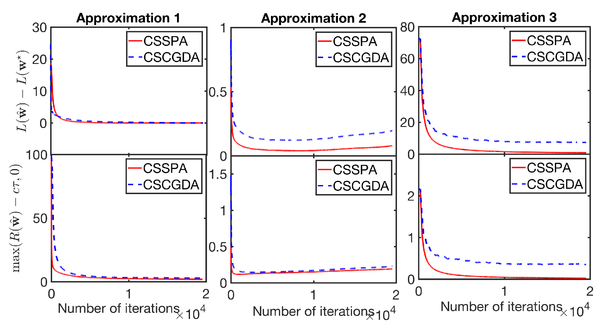
For the experiments, we consider the US Adult income dataset [45] available in the UCI Machine Learning Repository [46]. The dataset contains a total of 48,842 instances with the features for gender, race, education, occupation, working hours, etc. from the 1994 US Census. To each entry, we assign a label 1 if the income of adult is greater than or equal to $50,000 per annum and zero otherwise. The sensitive feature taken into account here is the gender. All the categorical features are converted into one-hot representations before training. Our goal here is to discern the label of an individual by looking at their features, while remaining fair to individuals across different genders. The three classifiers are learned with three different variants of the constraint as expressed in approximations. All the simulations are run in MATLAB. We consider of the whole data for tuning various parameters. By fixing , , , and at some random values, we first tune the constant and choose the step sizes , and . Later, we tune the other parameters , , , and to maximize the classification accuracy for each value of in Table II. Note that the values in Table II are obtained after solving the constrained optimization problem using an offline algorithm.
| 1 | 1.3270 | 1.3270 | 0.3 | |
| 1 | 2.0047 | 7.9810 | 0.25 | |
| 1 | 0.3972 | 6.2946 | 0.2 | |
| 1 | 1.6746 | 1.6746 | 0.15 | |
| 1 | 1.9953 | 7.9433 | 0.1 | |
| 1 | 0.3991 | 3.9905 | 0.05 |
For the results, we first present the trade-off between the risk difference and the classification loss achieved by the three approximations. All the classifiers are learned on the training data and the final graph in Fig. 2(a) is produced on testing data of 5-fold cross-validation data with instances. The empirical values of loss and risk difference are quantified on the testing data and are shown in Fig. 2(a). The trade-off curve is achieved by adjusting the parameters , , and appropriately as mentioned in Table II. As evident from the Fig. 2(a), the classifiers of all three approximations are able to achieve much lower possible risk difference values. Further, we observe that, approximation 2,3 generate better empirical loss than approximation 1 at lower risk difference values, which may be due to the higher estimation errors. Hence, the proposed classifiers are handy and can be tuned appropriately in oder to produce not more than the designer specified bias.
Next let us take a look at the evolution of the objective and constraint functions over the number of iterations for all three approximations. The performance of the proposed CSSPA algorithm is compared with the CSCGDA algorithm from [5]. To this end, we first solve the problem in an offline manner using the entire dataset. To this end, we use the trust-region reflective algorithm implemented within the ‘fmincon’ function in MATLAB. Fig. 2(b) shows the (running averages of the) optimality gap and the constraint violation against the number of iterations. As evident from the figure, the proposed algorithm beats CSCGDA in terms of the convergence rate.
IV-A4 Fair SpAM
Here, we apply CSSPA algorithm to solve SpAM problem with fairness constraints (see Sec. II-C). To this end, define , , , , as the known basis functions of , so that where are the coefficients. Hence the optimization problem boils down to finding the set of coefficients corresponding to each basis function as
| (33) |
Now we can write the objective function of the problem (IV-A4) in the required form as
and with linear constraints. Since all data points and basis functions are finite valued, we can ensure that , , , , and for all , and .

We test this application on a synthetic dataset. The dataset consists of 20,000 i.i.d. datapoints generated from a uniform distribution with 30 features each. We considered a model for simulations. The first 4 feature functions given by , , , are the only non-zero functions, where , , , and are coefficients randomly selected from . The sensitive feature is a linear transformation of the first feature, i.e., , where are randomly chosen from . The random variable is Gaussian with mean 0 and variance 0.1. The parameter is tuned by 5-fold cross-validation. In constraints we take . We have also implemented the CSCGDA method proposed in [5] and results are shown in Fig.3. To evaluate the performance of algorithms, we found the optimal solution by using ‘fmincon’ operator in MATLAB and use it to calculate the optimality gap. The step sizes are taken as mentioned in Table I. The experiment has been repeated over epochs using Monte Carlo method. The results in Fig.3 hence are averaged. It can be seen that the optimality gap and the constraint violation converge at a faster rate to zero for CSSPA, as compared to the method from [5].
V Conclusion
The constrained stochastic optimization problem with compositional objective and constraint functions is studied. The compositional form obviates the use of classical stochastic gradient-based methods that require unbiased gradient estimates. Likewise, the stochastic compositional gradient descent (SCGD) method cannot be used as it is meant for problems where projection over the constraint set can be easily computed. Hence a variant of the Arrow-Hurwicz saddle point algorithm is proposed where the expectation functions are tracked separately using auxiliary variables as estimated in the SCGD algorithm. A complete analysis with more general proof of convergence for convex problems is provided. The sample complexity of the proposed primal-dual algorithms is for the optimality gap after iterations while ensuring zero constraint violation. The derived rates here significantly outperform the best-known results for constrained stochastic compositional problems. Finally, the proposed algorithm is tested on two practical applications of classification and regression problems with enforced fairness constraints and is shown to be superior to the state-of-the-art algorithm.
Appendix A
Appendix B Preliminary Results
We begin with deriving some preliminary results. Consider the augmented Lagrangian for the surrogate problem (III-A),
| (34) |
To ensure that Slater’s condition is satisfied for (III-A), we will require that . The analysis proceeds by first bounding the optimality gap and the constraint violation by expressions that are functions of . At the final step, will be chosen so as to ensure that the constraint violation is zero.
Different from the analysis in [1] and its variants, the bounds here will contain term on the right. As no assumption is made on the boundedness of , these bounds are not equivalent to those in [1]. Instead, we will follow the approach of [47] wherein must be chosen so as to ensure that does not become too large. We begin with stating the following preliminary Lemma. For the analysis purpose, we define as the sigma algebra formed by random samples observed till time , i.e.,
| (35) |
Lemma 1.
The results in (36) and (37) bound the difference between consecutive primal and dual iterates. Of these, (36) follows from the boundedness of the gradients (Assumptions (A4) and (A6)) and the use of norm inequalities. Likewise, (37) follows from Assumption (A7). The recursive relationships in (38) and (39) characterize the tracking properties of the auxiliary variables and follow similarly as in [1, Lemma 2], except for the presence of the term. As stated earlier, since is not assumed to be bounded, the subsequent analysis will be different from [1]. For the sake of completeness, following contains the detailed proof.
Proof of (36).
Since , it follows from the non-expansiveness of the projection operator that
| (40) | ||||
| (41) |
where we have used the inequality and the triangle inequality. Taking conditional expectation in (41) given , and using the facts that is independent of and that is independent of , we obtain
| (42) | ||||
| (43) |
which is the required result. Note that the last inequality in (43) follows from the boundedness of the gradients (Assumptions (A4) and (A6)). ∎
Proof of (37).
We begin with using the triangle inequality for the term within the squares on the left-hand side of (37) as follows
| (44) |
for . Squaring (44). and bounding the cross-terms, we obtain
| (45) |
Finally, taking conditional expectation given and using the bounds in Assumptions (A5) and (A7), we obtain
| (46) |
which is the required result. ∎
Proof of (38) and (39).
Define and observe that it is bounded due to the continuity of (Assumption (A4)) as
| (47) |
From the definition of , we can write,
| (48) |
Here observe that . Therefore, squaring (48) and taking conditional expectation given , we obtain
| (49) |
where we have used the bound in Assumption (A4). Next, the Peter-Paul inequality implies that
| (50) | ||||
| (51) | ||||
| (52) |
where we have used the fact that . The inequality in (39) can also be derived in the similar fashion. ∎
We also state the following preliminary result that bounds the optimality gap of (III-A).
Lemma 2.
Lemma 2 follows from standard duality theory arguments, and its full proof can be found in [5, Appendix B].
Next, we give details on choices of various parameters and through the following lemma which will be utilized in proving convergence results.
Lemma 3.
Suppose the step sizes are selected as
- •
, , ,
- •
, ,
where , , and . For some constant , if we choose , and , then it holds
Proof.
We know for , it holds . Now consider the quadratic equation in as
| (53) |
For
| (54) |
where , we can say that the expression in (53) is non-positive. Since for , the choice of satisfies
Now, if we prove , it is sufficient to conclude that, the choice of stays in the interval as specified in (54) and . Consider
| (55) |
By substituting and in (B), we write
Since , , and , we conclude the proof by saying
∎
Appendix C Intermediate Results
We are now ready to derive the key lemmas relevant to the current proof. The bounds in the subsequent lemmas are stated using the big- notation, with the implicit understanding that the underlying constants depend only on the problem parameters , , , , , , , , , , , , and initialization of terms in Algorithm 1. We use the fact that the step-size parameters and are non-increasing, i.e., and according to the statements of Theorems 1, 2.
The following lemma is the first key result that glues the objective error and the constraint violation within a single inequality.
Lemma 4.
Let be any feasible solution to (III-A) and let . If the step sizes are selected such that , then we have the bound
| (56) |
The idea of bounding the left-hand side is borrowed from [13, Lemma 1]. However, the presence of non-linear functions of expectations on the left must be separately addressed using the techniques from [1]. The proof of Lemma 4 requires establishing five preliminary lemmas. In Lemmas 5 and 6, we use the primal update (4) and convexity of in to establish a bound on . Likewise, in Lemmas 7 and 8, we use the dual update (5) and strong concavity of with respect to to establish bound on . Lemma 4 would then follow by adding the results in Lemmas 6 and 8 and simplifying.
We begin with bounding the average decrement in where is a feasible point of (III-A).
Lemma 5.
For any feasible for (III-A), the following inequality holds with probability one:
| (57) |
Proof.
Since , it follows from the non-expansiveness of the projection operation that
| (58) | ||||
| (59) |
Let us denote
| (60) | ||||
| (61) |
Taking conditional expectation in (59) and using (36) from Lemma 1, we can write
| (62) |
Recalling that and , and using the definition of from (34), we obtain
| (63) | ||||
| (64) |
where we have used the convexity of with respect to ; see Assumption (A3). The term can be bounded by using the smoothness of (Assumption (A5)) and the Peter-Paul inequality as follows:
| (65) | ||||
| (66) | ||||
| (67) | ||||
| (68) | ||||
| (69) |
where we have used the compactness of (Assumption (A2)) in (68) and the boundedness of the gradient (Assumption (A4)) in (69). Proceeding along similar lines and again using Assumptions (A5), (A2), and (A4), we obtain
| (70) |
Substituting the expressions (69) and (70) in (64), we obtain the required result. ∎
Let initial tracking errors are denoted as and and is denotes as . Building up on the result in Lemma 5, we bound the total Lagrangian deviation.
Proof.
Next, we derive the corresponding results for the dual variable using the updates in (5).
Lemma 7.
For any , if the step sizes are chosen as then the following inequality holds with probability one:
| (74) |
Proof.
Since , we can write
| (75) | ||||
| (76) | ||||
| (77) |
where the term can be bounded by using the smoothness of (Assumption (A5)) so as to yield
| (78) | ||||
| (79) | ||||
| (80) | ||||
| (81) |
Here, (79) follows from the Cauchy-Schwartz inequality while (81) follows from the Peter-Paul inequality. Taking conditional expectation given in (77), and recalling that , we obtain
| (82) | ||||
| (83) |
where we have substituted (81). Since is strongly-concave in , we have that
| (84) | ||||
| (85) |
where the last inequality is followed by (37). From the statement of Lemma 4, since , we also have . Therefore we can write in (85). ∎
Proof.
Having established the basic results, we are ready to prove Lemma 4.
Proof of Lemma 4.
From the definition of in (34), we have that
| (89) |
where (89) follows from the fact that and for all . Now from Lemmas 6 and 8, we can write
| (90) |
For the sake of brevity, we define
| (91) | ||||
| (92) |
Now by interchanging the terms, we can write
| (93) |
By the statement of Lemma 3, the first term on the RHS is negative if we choose . Finally, by rearranging the terms and ignoring the constants, we obtain the required result. ∎
Appendix D Proof of Theorem 1
To prove almost sure convergence for the unconstrained version of ( P ), the coupled Supermartingale Convergence Theorem has been used in [1, Theorem 5]. In the current context however, since we have not assumed anything on the boundedness of , the same cannot be used. Instead, we use different approach, wherein we add the various quantities in (5), (7), (38), and (39), and study the convergence of the resulting sequence. Then, by applying Supermartingale Convergence Theorem [48] to that cumulative sequence, we prove is bounded for all with probability 1. Subsequently, we apply Supermartingale Convergence Theorem to each of the sequences individually and obtain the required result.
We begin by combining the statements of Lemmas 5 and 7, to obtain
| (94) |
Let us define
| (95) |
Multiplying (38), (39) by and adding with (94), we obtain
| (96) |
For the sake of brevity, let us define
| (97) |
so that
| (98) |
From (89), we can write
which by substituting back in (D), we get
| (99) |
The result in (D) holds for any feasible point. Note that, from the statement of Theorem 1, it is given in (III-A). Hence, both of the problems in ( P ) and (III-A) are equivalent, which implies any feasible point to (III-A) is also feasible to ( P ). Hence we replace by the saddle point which is the optimal solution pair of primal problem in ( P ), and dual problem in (7)
| (100) |
Defining , and , and rearranging the terms, we can write,
| (101) |
| (102) |
where the inequality follows from (36). Now, by again defining , we write
| (103) |
Observe that is a convex quadratic function of and from Lemma 3, it can be made non-positive, if we choose
Hence . Now by dropping in (103) and substitute , we obtain
| (104) |
Since is the saddle point, by KKT conditions, we have that
| (105) | ||||
| (106) |
or equivalently for any and ,
| (107) |
Since due to the complementary slackness condition, the sequence in (104) is non negative. Recall from Assumption A2 that is bounded. Therefore from the step-size choices made in the statement of Theorem 1, the sequences and are summable with probability 1. Applying the Supermartingale Convergence Theorem to (104), we can say the converges almost surely to a nonnegative random variable, and with probability 1. Therefore we have that
| (108) |
Since converges almost surely, the sequences , must be bounded with probability 1, and consequently, the component sequences , , , and are also bounded with probability 1. Next, observe that can be written as
| (109) | ||||
| (110) |
where note that the sequence is summable and is finite. Therefore, from the Supermartingale Convergence Theorem, it follows that is almost surely convergent to a non negative random variable. Further, the Monotone Convergence Theorem implies that with probability one. Now consider
| (111) | ||||
| (112) |
since and are summable, it follows from the almost Supermartingale Convergence Theorem that and are almost surely convergent to some non negative random variables, and further we have
| (113) | ||||
| (114) |
which also implies that
| (115) |
Since , , , are almost surely convergent, we can conclude is also almost surely convergent to a non negative random variable. Let and , where is the set of primal and dual optimal pairs. We have established that for any , the sequence converge almost surely to a non negative random variable. for any , let be a sample path such that exists, and is the collection of all such paths . For any , It implies that .
The following lemma establishes that, the sequence converges almost surely to any optimal solution.
Lemma 9.
Let . Then is convergent for all with probability 1.
The proof is provided in [1, Theorem 1(a), page 13-14].
Before concluding the proof we explain the implication of the statements of Lemma 9. Consider an arbitrary sample trajectory of such that and . For any arbitrary , since converges, the sequence is bounded. By continuity of , the sequence must have a limit point such that . Observe from (105), it is clear that, is the minimizer of of any . Hence occurs only at which is an optimal solution of ( P ). Since , we can say is also a convergent sequence. Since it is convergent with limit point 0, we have . Then on this sample trajectory. Note that set of all sample paths has a probability measure of one. Hence we complete the proof by concluding, almost surely converges to a random point in the set of optimal solutions of ( P ).
Appendix E Proof of Theorem 2
The proof is divided into two parts. In the first part we choose , and to prove convergence of objective error. Later, we choose , and to prove convergence of constraint violation. As a first step we analyze the optimality gap. Recall that from Lemma 7, the results here are hold for any , and feasible point s.t . Since is also a feasible point to the problem (III-A), for the first result, we choose and . Substituting into (56), we obtain
| (116) |
Let and for large , we can approximate as when . Since is a convex function we can write
| (117) | ||||
| (118) |
where the first step in (117) is obtained by adding and subtracting , and the final step in (118) follows from Lemma 2.
Next, we choose which is dual optimum of the problem (III-A), i.e.,
| (119) |
Since is the optimal solution of primal problem in (III-A), and , from assumption A2, the pair constitutes a saddle point of the problem (III-A), and satisfies KKT conditions
| (120) | ||||
| (121) |
or equivalently, for any , and ,
| (122) |
For the ease of analysis, we write the classical definition of Lagrangian function for the problem in (III-A) as
| (123) |
Let be a vector in which entry is unity and zeros elsewhere. Then
| (124) | ||||
| (125) |
By rearranging the terms, we write
| (126) |
From the observation in (122), we can say . Hence we can write
| (127) | ||||
| (128) |
The second inequality follows from the complementary slackness condition
.
Since the result in Lemma 4 holds for any , we can replace by . Hence by summing over , we can rewrite (127) as
where the last step follows from the bound on in Lemma 2. Finally the required order bound on can be obtained simply by substituting the constant/diminishing step-sizes and ignoring all constant terms.
References
- [1] M. Wang, E. X. Fang, and H. Liu, “Stochastic compositional gradient descent: algorithms for minimizing compositions of expected-value functions,” Mathematical Programming, vol. 161, no. 1-2, pp. 419–449, 2017.
- [2] M. Wang, J. Liu, and E. X. Fang, “Accelerating stochastic composition optimization,” J. Mach. Learn. Res., vol. 18, no. 1, pp. 3721–3743, 2017.
- [3] M. Wang and J. Liu, “A stochastic compositional gradient method using markov samples,” in Proc. IEEE WSC, Dec. 2016, pp. 702–713.
- [4] S. Ghadimi, A. Ruszczynski, and M. Wang, “A single timescale stochastic approximation method for nested stochastic optimization,” SIAM Journal on Optimization, vol. 30, no. 1, pp. 960–979, 2020.
- [5] S. T. Thomdapu and K. Rajawat, “Optimal design of queuing systems via compositional stochastic programming,” IEEE Trans. Commun., vol. 67, no. 12, pp. 8460–8474, 2019.
- [6] ——, “Optimizing qos for erasure-coded wireless data centers,” in Proc. IEEE ICC, June, 2021, pp. 1–6.
- [7] Z. Akhtar, A. S. Bedi, and K. Rajawat, “Conservative stochastic optimization with expectation constraints,” IEEE Trans. Signal Process., vol. 69, pp. 3190–3205, 2021.
- [8] X. Wang and N. Gao, “Stochastic resource allocation over fading multiple access and broadcast channels,” IEEE Trans. Inf. Theory, vol. 56, no. 5, pp. 2382–2391, 2010.
- [9] A. Ribeiro, “Ergodic stochastic optimization algorithms for wireless communication and networking,” IEEE Trans. Signal Process., vol. 58, no. 12, pp. 6369–6386, 2010.
- [10] X. Wang and G. B. Giannakis, “Resource allocation for wireless multiuser OFDM networks,” IEEE Trans. Inf. Theory, vol. 57, no. 7, pp. 4359–4372, 2011.
- [11] S. T. Thomdapu, P. Katiyar, and K. Rajawat, “Dynamic cache management in content delivery networks,” Computer Networks, vol. 187, p. 107822, 2021.
- [12] A. Nedić and A. Ozdaglar, “Subgradient methods for saddle-point problems,” J. of Opt. Theory and Applications., vol. 142, no. 1, pp. 205–228, 2009.
- [13] A. Koppel, F. Y. Jakubiec, and A. Ribeiro, “A saddle point algorithm for networked online convex optimization,” IEEE Trans. Signal Process., vol. 63, no. 19, pp. 5149–5164, 2015.
- [14] A. S. Bedi, A. Koppel, and K. Rajawat, “Beyond consensus and synchrony in decentralized online optimization using saddle point method,” in Proc. IEEE Asilomar, 2017, pp. 293–297.
- [15] H. Yu, M. Neely, and X. Wei, “Online convex optimization with stochastic constraints,” in Advances in Neural Information Processing Systems, 2017, pp. 1428–1438.
- [16] A. S. Bedi, A. Koppel, and K. Rajawat, “Asynchronous saddle point algorithm for stochastic optimization in heterogeneous networks,” IEEE Trans. Signal Process., vol. 67, no. 7, pp. 1742–1757, 2019.
- [17] A. N. Madavan and S. Bose, “Subgradient methods for risk-sensitive optimization,” arXiv preprint arXiv:1908.01086, 2019.
- [18] A. Benveniste, M. Métivier, and P. Priouret, Adaptive algorithms and stochastic approximations. Springer Science & Business Media, 2012, vol. 22.
- [19] D. P. Bertsekas and J. N. Tsitsiklis, Parallel and distributed computation: numerical methods. Prentice hall Englewood Cliffs, NJ, 1989, vol. 23.
- [20] V. S. Borkar, Stochastic approximation: a dynamical systems viewpoint. Springer, 2009, vol. 48.
- [21] D. Dentcheva, S. Penev, and A. Ruszczyński, “Statistical estimation of composite risk functionals and risk optimization problems,” Springer Journal on Annals of the Institute of Statistical Mathematics, vol. 69, no. 4, pp. 737–760, 2017.
- [22] X. Lian, M. Wang, and J. Liu, “Finite-sum composition optimization via variance reduced gradient descent,” in Proc. Artificial Intel. and Stats., Apr. 2017, pp. 1159–1167.
- [23] A. Koppel, A. S. Bedi, and K. Rajawat, “Controlling the bias-variance tradeoff via coherent risk for robust learning with kernels,” in Proc. IEEE ACC, May, 2019, pp. 3519–3525.
- [24] B. Dai, N. He, Y. Pan, B. Boots, and L. Song, “Learning from conditional distributions via dual embeddings,” in Artificial Intelligence and Statistics, 2017, pp. 1458–1467.
- [25] Y. Hu, S. Zhang, X. Chen, and N. He, “Biased stochastic gradient descent for conditional stochastic optimization,” arXiv preprint arXiv:2002.10790, 2020.
- [26] A. S. Bedi and K. Rajawat, “Asynchronous incremental stochastic dual descent algorithm for network resource allocation,” IEEE Trans. Signal Process., vol. 66, no. 9, pp. 2229–2244, 2018.
- [27] T. Chen, A. Mokhtari, X. Wang, A. Ribeiro, and G. B. Giannakis, “Stochastic averaging for constrained optimization with application to online resource allocation,” IEEE Trans. Signal Process., vol. 65, no. 12, pp. 3078–3093, 2017.
- [28] X. Wang, X. Chen, T. Chen, L. Huang, and G. B. Giannakis, “Two-scale stochastic control for integrated multipoint communication systems with renewables,” IEEE Trans. Smart Grid, vol. 9, no. 3, pp. 1822–1834, 2016.
- [29] T. Chen, S. Barbarossa, X. Wang, G. B. Giannakis, and Z.-L. Zhang, “Learning and management for internet of things: Accounting for adaptivity and scalability,” Proc. of the IEEE, vol. 107, no. 4, pp. 778–796, 2019.
- [30] A. Ruszczyński and A. Shapiro, “Optimization of convex risk functions,” Mathematics of operations research, vol. 31, no. 3, pp. 433–452, 2006.
- [31] M. B. Zafar, I. Valera, M. Gomez Rodriguez, and K. P. Gummadi, “Fairness beyond disparate treatment & disparate impact: Learning classification without disparate mistreatment,” in Proc. intl. conf. on world wide web, 2017, pp. 1171–1180.
- [32] G. Goh, A. Cotter, M. Gupta, and M. P. Friedlander, “Satisfying real-world goals with dataset constraints,” in Advances in Neural Information Processing Systems, 2016, pp. 2415–2423.
- [33] T. Kamishima, S. Akaho, and J. Sakuma, “Fairness-aware learning through regularization approach,” in Proc. IEEE Intl. Conf. on Data Mining Workshops, 2011, pp. 643–650.
- [34] A. K. Menon and R. C. Williamson, “The cost of fairness in binary classification,” in Proc. Conf. on Fairness, Accountability and Transparency, 2018, pp. 107–118.
- [35] M. Olfat and A. Aswani, “Spectral algorithms for computing fair support vector machines,” in Proc. Intl. Conf. on Artificial Intel. Stat., 2018, pp. 1933–1942.
- [36] B. Woodworth, S. Gunasekar, M. I. Ohannessian, and N. Srebro, “Learning non-discriminatory predictors,” in Proc. Conf. on Learning Theory, 2017, pp. 1920–1953.
- [37] M. B. Zafar, I. Valera, M. Gomez-Rodriguez, and K. P. Gummadi, “Fairness constraints: A flexible approach for fair classification.” J. Mach. Learn. Res., vol. 20, no. 75, pp. 1–42, 2019.
- [38] Y. Wu, L. Zhang, and X. Wu, “On convexity and bounds of fairness-aware classification,” in Proc. The World Wide Web Conference, 2019, pp. 3356–3362.
- [39] D. Pedreschi, S. Ruggieri, and F. Turini, “A study of top-k measures for discrimination discovery,” in Proc. ACM Symposium on Applied Computing, 2012, pp. 126–131.
- [40] J. Komiyama, A. Takeda, J. Honda, and H. Shimao, “Nonconvex optimization for regression with fairness constraints,” in International conference on machine learning, 2018, pp. 2737–2746.
- [41] R. Berk, H. Heidari, S. Jabbari, M. Joseph, M. Kearns, J. Morgenstern, S. Neel, and A. Roth, “A convex framework for fair regression,” arXiv preprint arXiv:1706.02409, 2017.
- [42] P. Ravikumar, J. Lafferty, H. Liu, and L. Wasserman, “Sparse additive models,” Journal of the Royal Statistical Society: Series B (Statistical Methodology), vol. 71, no. 5, pp. 1009–1030, 2009.
- [43] A. Zink and S. Rose, “Fair regression for health care spending,” Biometrics, 2019.
- [44] R. Tibshirani, “Regression shrinkage and selection via the lasso,” Journal of the Royal Statistical Society: Series B (Methodological), vol. 58, no. 1, pp. 267–288, 1996.
- [45] “Adult income,” 1996. [Online]. Available: https://archive.ics.uci.edu/ml/datasets/adult
- [46] D. Dua and C. Graff, “UCI machine learning repository,” 2017. [Online]. Available: http://archive.ics.uci.edu/ml
- [47] A. Koppel, B. M. Sadler, and A. Ribeiro, “Proximity without consensus in online multiagent optimization,” IEEE Trans. Signal Process., vol. 65, no. 12, pp. 3062–3077, 2017.
- [48] H. Robbins and D. Siegmund, “A convergence theorem for non negative almost supermartingales and some applications,” in Optimizing methods in statistics. Elsevier, 1971, pp. 233–257.