Node Failure Localization: Theorem Proof

For Algorithm 1, the input network is not necessarily a connected graph. Lemma II.1, however, only considers the case that the input network satisfying the three conditions (in Lemma II.1) is connected. Then it suffices to show that Algorithm 1 places the minimum number of monitors to ensure that any two non-monitors in $\mathcal{G}^{\prime}$ (satisfying the three conditions in Lemma II.1) are distinguishable. Such connected input network can be represented as a tandem network¹¹ 1 In this report, networks with such structures are called tandem networks., shown in Fig. 1. As illustrated in Fig. 1, suppose there are $z$ biconnected components in $\mathcal{G}^{\prime}$, where $\mathcal{B}_{1}$ and $\mathcal{B}_{z}$ have external monitor connections via $v_{0}$ and $v_{z}$ to $m_{1}$ and $m_{2}$ outside $\mathcal{G}^{\prime}$.

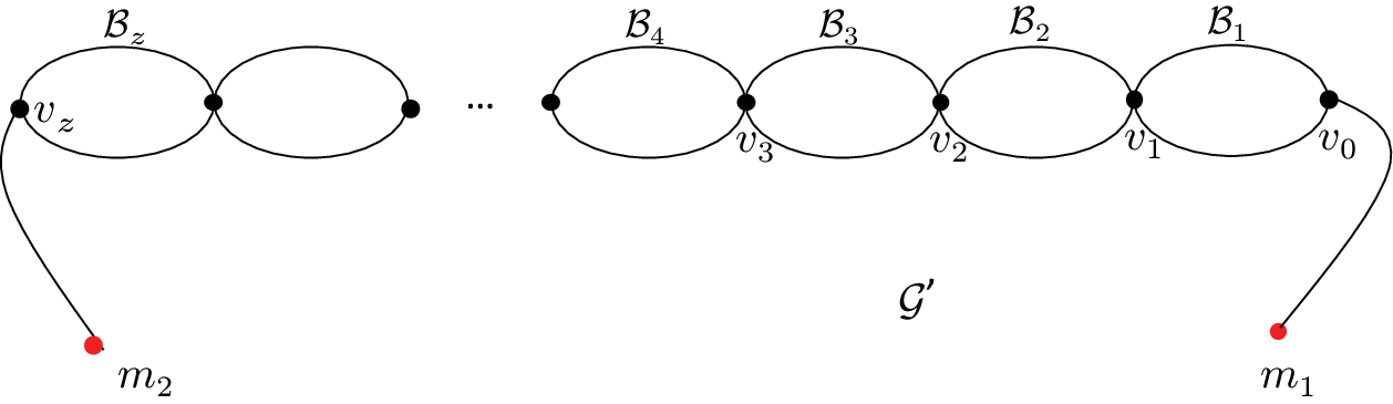
(1) We first prove that any non-cut-vertex (excluding the nodes connecting to external monitors, e.g., $v_{0}$ and $v_{z}$ in Fig. 1), denoted by $w$, in $\mathcal{G}^{\prime}$ is 1-identifiable if $\exists$ another monitor, denoted by $m_{3}$, in $\mathcal{G}^{\prime}$ ($m_{3}$ can be anywhere in $\mathcal{G}^{\prime}$).

(1.a) The case that $m_{1}\neq m_{2}$. Suppose $w$ is in biconnected component $\mathcal{B}_{i}$. Then according to Theorem 15 [1], $w$ is distinguishable from any other node (including cut-vertices or nodes connecting to external monitors) in $\mathcal{B}_{i}$. Moreover, for a node outside $\mathcal{B}_{i}$, say $u$, it is impossible that measurement path (from $m_{1}$ to $m_{2}$ in Fig. 1) must go through $u$ and $w$ at the same time, since $w$ must be a cut-vertex in Fig. 1 otherwise, contradicting the assumption. Therefore, $w$ is also distinguishable from nodes outside $\mathcal{B}_{i}$. Thus, $w$ is 1-identifiable when $m_{1}\neq m_{2}$ even without $m_{3}$.

(1.b) The case that $m_{1}=m_{2}$. To ensure each node in $\mathcal{G}^{\prime}$ is 1-identifiable, at least one extra monitor (besides $m_{1}$ and $m_{2}$) that can generate simple measurement paths traversing $\mathcal{G}^{\prime}$ is required. Now we have monitor $m_{3}$ in $\mathcal{G}^{\prime}$. In this case, $\mathcal{G}^{\prime}$ can be further decomposed into subgraphs. Then the argument in (1.a) applies to each subgraph by using $m_{3}$.

In sum, $w$ is 1-identifiable in $\mathcal{G}^{\prime}$, i.e., any non-cut-vertex (excluding the nodes connecting to external monitors) in $\mathcal{G}^{\prime}$ is 1-identifiable if $\exists$ a monitor in $\mathcal{G}^{\prime}$.

(2) Based on the argument in (1), we know that additional monitor placement (besides $m_{1}$ and $m_{2}$ in Fig. 1) in $\mathcal{G}^{\prime}$ is only for distinguishing the cut-vertices and nodes connecting to external monitors. Now we consider how to place the minimum number (at least one monitor, thus the argument in (1.b) still holds) of monitors to distinguish all these nodes in $\mathcal{G}^{\prime}$. In Algorithm 1, line 1 assigns a sequence number to each biconnected component. This is feasible as $\mathcal{G}^{\prime}$ is a tandem network. Suppose $|\mathcal{B}_{i}|\geq 3$ (i.e., $\mathcal{B}_{i}$ is not bond). Then, as Fig. 1 illustrates, to ensure the 1-identifiability of $v_{0}$, there are three possible locations for necessary monitor placement: (i) $v_{0}$ connects to another external monitor; (ii) place a monitor in $\mathcal{B}_{1}$; or (iii) select a monitor from $V(\mathcal{B}_{2})\setminus\{v_{2}\}$. Similarly, there are also three possible locations for monitor placement such that $v_{1}$ and $v_{2}$ are 1-identifiable. To ensure the 1-identifiability of $v_{0}$, $v_{1}$, and $v_{2}$, we notice that there exists a common location, i.e., a node in $V(\mathcal{B}_{2})\setminus\{v_{1},v_{2}\}$, where placing one monitor can guarantee that $v_{0}$, $v_{1}$, and $v_{2}$ are all 1-identifiable. Moreover, no other places can guarantee that $v_{0}$, $v_{1}$, and $v_{2}$ are 1-identifiable at the same time. Thus, line 1 selects a monitor, denoted $m_{3}$, from $V(\mathcal{B}_{2})\setminus\{v_{1},v_{2}\}$. Note that the selection of $m_{3}$ only guarantees that $v_{0}$, $v_{1}$, and $v_{2}$ are 1-identifiable, i.e., the identifiability of all other nodes remain the same. Hence, $m_{3}$ does not affect the necessity of previously deployed monitors. However, if $\mathcal{B}_{2}$ is a bond and $\mathcal{B}_{1}$ is not a bond, then to ensure that $v_{0}$ is 1-identifiable, there are only two possible locations for monitor placement: (i) $v_{0}$ connects to another external monitor or (ii) place a monitor in $\mathcal{B}_{1}$. Meanwhile, to ensure that $v_{1}$ is 1-identifiable, the possible monitor locations are also reduced to two: (i) place a monitor in $\mathcal{B}_{1}$ or (ii) place a monitor in $\mathcal{B}_{3}$. In such case, the common location to ensure the 1-identifiability of both $v_{0}$ and $v_{1}$ is in $\mathcal{B}_{1}$. Thus, line 1 deploys a monitor at the common node between $\mathcal{B}_{1}$ and $\mathcal{B}_{2}$. As aforementioned, for this newly selected monitor, it is only for identifying a specific set of nodes. All previously deployed monitors remain necessary. After this placement, lines 1 and 1 remove the processed biconnected components. Then the remaining graph is processed by Algorithm 1 recursively, as further monitor placement is independent of the monitors that are already deployed. Finally, one trivial case we have not discussed is that $\mathcal{G}_{i}$ contains only one biconnected component, where a randomly chosen monitor (line 1) can ensure the network 1-identifiability. Therefore, for the input network satisfying the conditions in Lemma II.1, Algorithm 1 can place the minimum number of monitors for achieving the network 1-identifiability. $\blacksquare$

First, we consider the case that the input connected network is not 2-connected. In this case, there exist at least one cut-vertex and two biconnected components, and auxiliary algorithm Algorithm 3 is not invoked. For such input network, we discuss it as follows.

(1) We first place necessary monitors in each biconnected component. If biconnected component $\mathcal{B}_{i}$ has only one cut-vertex, denoted by $v_{c}$, then at least one non-cut-vertex in $\mathcal{B}_{i}$ should be a monitor.

(1.a) If $\mathcal{B}_{i}$ is a PLC, then we can randomly select a non-cut-vertex, denoted by $m_{i}$, as a monitor (line 2) according to Theorem 15 and Corollary 16 [1], such that any node $w$ with $w\in V(\mathcal{B}_{i})\setminus\{v_{c}\}$ is distinguishable from any node in $V(\mathcal{B}_{i})$. Moreover, $w$ is also distinguishable from nodes outside $\mathcal{B}_{i}$ due to the existence of path from $m_{i}$ to $v_{c}$ without traversing $w$. Therefore, all nodes in $V(\mathcal{B}_{i})\setminus\{v_{c}\}$ are 1-identifiable when $\mathcal{B}_{i}$ is a PLC and has only one cut-vertex.

(1.b) If $\mathcal{B}_{i}$ is not a PLC, i.e., $\mathcal{B}_{i}$ contains at least one polygon, then the required monitor in $\mathcal{B}_{i}$ cannot be randomly placed. For this case, we need to first find all nodes in $\mathcal{B}_{i}$ that are guaranteed to be 1-identifiable. For these 1-identifiable nodes, there are three cases:

1. \small1⃝

   A PLC with 3 or more agents. As shown in Fig. 2, PLC $\Lambda_{1}$ has three agents and $\mathcal{B}_{i}$ must have a monitor (say $m_{\mathcal{B}_{i}}$) that is not $v_{c}$. Moreover, outside $\mathcal{B}_{i}$, $v_{c}$ must connect to a monitor, e.g., a monitor in $\Lambda_{4}$ (denoted by $m_{\Lambda_{4}}$). Within $\Lambda_{1}$, for any two nodes $w_{1}$ and $w_{2}$ ($w_{1}\neq w_{2}\neq v_{c}$), we can find a path traversing only $w_{1}$ but not $w_{2}$ (and vice versa) using $m_{\mathcal{B}_{i}}$ and $m_{\Lambda_{4}}$ as $\Lambda_{1}$ is a PLC. Therefore, each node in $V(\Lambda_{1})\setminus\{v_{c}\}$ is 1-identifiable. Then following the similar argument in (1) of Section III-A, we know each node in $V(\Lambda_{3}+\Lambda_{2})\setminus\{v_{1},v_{2},v_{3},v_{4}\}$ is 1-identifiable, where $\Lambda_{2}$ and $\Lambda_{3}$ are the neighboring PLCs of $\Lambda_{1}$. Therefore, to ensure that all non-cut-vertices are 1-identifiable, monitor placement in $\mathcal{B}_{i}$ only needs to make sure that nodes in $\mathcal{B}^{*}_{i}$ (see Fig. 2) are 1-identifiable. However, $\mathcal{B}^{*}_{i}$ may not be a tandem network, i.e., $\mathcal{B}^{*}_{i}$ possibly contains a polygon, which needs to be further processed in the following cases.

2. \small2⃝

   A PLC with 4 or more neighboring PLCs. This case is illustrated in Fig. 3. In Fig. 3, $\Lambda_{1}$ has two neighboring polygons, which implies that $\Lambda_{1}$ has 4 or more neighboring PLCs. In this case, $\mathcal{U}_{1}$ must have at least one monitor, since $v_{5}$ and $v_{6}$ are not distinguishable otherwise. Similarly, $\mathcal{U}_{2}$ must also have a monitor. Using these two monitors, every node in $\Lambda_{1}$ can be shown to be 1-identifiable as $\Lambda_{1}$ is a PLC. Then following the similar argument in (1) of Section III-A, we know each node in $V(\Lambda_{2}+\Lambda_{3}+\Lambda_{4}+\Lambda_{5})\setminus\{v_{j}\}^{8}_{j=5}$ is 1-identifiable, where $\Lambda_{2}$, $\Lambda_{3}$, $\Lambda_{4}$, and $\Lambda_{5}$ are the neighboring PLCs of $\Lambda_{1}$.

3. \small3⃝

   A PLC with 2 agents and one agent is a cut-vertex. This case is shown in Fig. 4. Following the similar argument in (1) of Section III-A, we know that each node in $V(\Lambda_{1}+\Lambda_{2})\setminus\{v_{1},v_{2},v_{c}\}$ is 1-identifiable, where $\Lambda_{1}$ and $\Lambda_{2}$ have the common node $v_{c}$. However, $v_{1}$ and $v_{2}$ may or may not be distinguishable depending on the topology of $\mathcal{B}^{*}_{i}$.

Lines 2–2 consider the above three cases to remove all 1-identifiable nodes²² 2 $v_{c}$ in Fig. 2 and Fig. 4 is also temporarily removed; however, it still exists in neighboring biconnected components, and thus the 1-identifiability of $v_{c}$ will be considered later in lines 2–2.. Note that in lines 2–2, we get sets $A$, $C$, and $E$, the common non-cut-vertices among these three sets may not be marked as 1-identifiable in any of the above three cases. Nevertheless, we can prove these common non-cut-vertices are also 1-identifiable as follows: Let $U_{c}$ be the set containing all such common non-cut-vertices, and $U_{r}=A\cup C\cup E\setminus U_{c}$. Now consider a random node $z$ with $z\in U_{c}$ and another node $x$. There are 3 cases: (i) If $x\in U_{r}$, then we know $x$ is distinguishable from $z$ based on previous results; (ii) if $x\in U_{c}$, then $\exists$ a path traversing $x$ without going through $z$ using nodes in sets $A$, $C$, and $E$; (iii) if $x\notin U_{r}\cup U_{c}$, then as (ii) shows that $z$ and $x$ are also distinguishable because of the existence of paths bypassing $z$ using nodes in $U_{r}\cup U_{c}$. Therefore, the common non-cut-vertex $z$ is 1-identifiable. Using this union set $A\cup C\cup E$, the remaining graph obtained by line 2 is a collection of tandem networks. Within this collection of tandem networks, consider two non-monitors $w_{1}$ and $w_{2}$ in two different connected tandem networks. We can show that $w_{1}$ and $w_{2}$ are distinguishable. This is because each connected tandem network must have additional necessary monitors. Using these additional monitors and also the removed components, we can find paths traversing only $w_{1}$ or $w_{2}$. Moreover, for these additional monitors, each has at least two internally vertex disjoint paths to any cut-vertex in the parent biconnected component. Thus, each non-monitor in one of these connected tandem network is distinguishable from any non-monitor outside its parent biconnected component. Therefore, it suffices to only consider how to enable the 1-identifiability in each of these connected tandem networks. This goal can be achieved by Algorithm 1, the correctness of which is shown in Lemma II.1.

(2) In processing each biconnected component, we only place the necessary monitors. These necessary monitor placements are proved to be able to ensure that all non-cut-vertex nodes in biconnected components are 1-identifiable. Next, we can consider the 1-identifiability of cut-vertices. Note that for a biconnected component, if no necessary monitors are placed so far, that means this biconnected component is either a PLC or contains a sufficient number of cut-vertices so that no additional monitors are required. For these biconnected components without monitors, it is still possible to find 1-identifiable cut-vertices in the following two cases:

1. \small1⃝

   A biconnected component with 2 cut-vertices and 3 or more neighboring biconnected components, such as $\mathcal{B}_{1}$ in Fig. 5. In this case, we know that $v_{2}$ must have two monitor connections, one through $\mathcal{B}_{2}$ and the other through $\mathcal{B}_{3}$. Meanwhile, $v_{1}$ also has a monitor connection through $\mathcal{B}_{4}$. Using these monitor connections, each node in $V(\mathcal{B}_{1})\setminus\{v_{1}\}$ is 1-identifiable. Note that unlike our previous discussion in (1) that connecting point may not be 1-identifiable. In Fig. 5, cut-vertex $v_{2}$ is guaranteed to be 1-identifiable, because it has more than two internally vertex disjoint monitor connections.

2. \small2⃝

   A biconnected component with 3 or more cut-vertices, such as $\mathcal{B}_{1}$ in Fig. 6. In this case, $v_{i}$ ($i=\{2,3,4\}$) must have a monitor connection through $\mathcal{B}_{i}$. Using these monitor connections, all nodes in $\mathcal{B}_{1}$ (including the cut-vertices) are 1-identifiable. Similarly, nodes in $V(\mathcal{B}_{2}+\mathcal{B}_{3}+\mathcal{B}_{4})\setminus\{v_{5},v_{6},v_{7}\}$ are also 1-identifiable, where $\mathcal{B}_{2}$, $\mathcal{B}_{3}$, and $\mathcal{B}_{4}$ are neighboring biconnected components of $\mathcal{B}_{1}$.

Lines 2–2 consider all above cases to determine the 1-identifiable nodes. Removing the 1-identifiable nodes by line 2, we get a collection of tandem networks without containing any monitors. Following our previous arguments about monitor placement in a collection of tandem networks (arguments after \small3⃝ in (1)), we further deploy monitors optimally by lines 2–2.

In this way, we use the minimum number of monitors to ensure that any cut-vertex is 1-identifiable in a given non-2-connected network.

Finally, we consider the case that the input connected network is 2-connected. In this case, there are no cut-vertices. However, it is still possible to determine some 1-identifiable nodes. Specifically, Case-\small2⃝ in (1) can be applied to 2-connected network $\mathcal{G}$ with 2 or more polygons. This particular case is handled by line 3–3 in Algorithm 3. However, if no 1-identifiable nodes can be found, then it implies that 2-connected $\mathcal{G}$ itself is a PLC or contains one and only one polygon. If the given 2-connect network is a PLC, then randomly selecting two monitors (line 3 of Algorithm 3) can ensure network 1-identifiability according to Theorem 15 [1]. While for a 2-conencted network with one and only one polygon, our strategy is to deploy the first monitor, remove the 1-identifiable nodes using our previous methods in Algorithm 2, and then apply Algorithm 1 to optimally deploy monitors in the remaining graph. For a 2-connected network with only one polygon, there are two cases:

1. \small1⃝

   All PLCs in $\mathcal{G}$ are non-bonds. For this case, there is no difference in selecting which PLC to deploy the first monitor because all PLCs have the same structure with at least one non-agent node. This case is captured by lines 3–3 in Algorithm 3.

2. \small2⃝

   $\exists$ at least one bond in $\mathcal{G}$. In this case, we randomly select a bond PLC, denoted by $\Lambda^{\prime}$ with two end-points $v_{1}$ and $v_{2}$ and two neighboring PLCs $\Lambda_{1}$ ($v_{1}\in\Lambda_{1}$) and $\Lambda_{2}$ ($v_{2}\in\Lambda_{2}$), shown in Fig. 7. To distinguish $v_{1}$ and $v_{2}$ in Fig. 7, we need a monitor in $\Lambda_{1}$ or $\Lambda_{2}$ or both. Depending on if $\Lambda_{1}$ or $\Lambda_{2}$ is a bond, we have to select $v_{1}$ or $v_{2}$ as a monitor. To get such monitor candidates, we use lines 3–3 to get $w_{1}$ and $w_{2}$ for possibly placing the first monitor. Unfortunately, we have no knowledge on which one (selecting $w_{1}$ or $w_{2}$ as a monitor) can generate the optimal solution. Therefore, we test them both, and select the one with the minimum number of monitors as the final output; see lines 3–3 of Algorithm 3.

In all, the above discussion on 2-connected input network is complete to cover all cases of 2-connected networks.

Consequently, OMP-CSP (Algorithm 2) can guarantee network 1-identifiability using the minimum number of monitors for any given network topology. $\blacksquare$

References

- [1] L. Ma, T. He, A. Swami, D. Towsley, and K. K. Leung, “On optimal monitor placement for localizing node failures via network tomography,” in IFIP WG 7.3 Performance, 2015.
- [2] R. Diestel, Graph theory. Springer-Verlag Heidelberg, New York, 2005.