跳到论文正文
W Papers独立论文阅读器 arXiv:2012.09351 论文正文 计算阅读时间 · 0%
引用这篇论文根据当前论文元数据生成,正式投稿前建议核对。


License: CC BY 4.0
arXiv:2012.09351v2 [cs.IT] 28 Dec 2020

Battle between Rate and Error in Minimizing Age of InformationDOI: 10.1145/1122445.1122456Conference: Woodstock ’18: ACM Symposium on Neural Gaze Detection; June 03–05, 2018; Woodstock, NYPrice: 15.00ISBN: 978-1-4503-XXXX-X/18/06

Guidan Yao Affiliation: The Ohio State University email: yao.539@osu.edu , Ahmed M. Bedewy Affiliation: The Ohio State University email: bedewy.2@osu.edu and Ness B. Shroff Affiliation: The Ohio State University email: shroff.11@osu.edu
2018© , 2018;
Abstract.

In this paper, we consider a status update system, in which update packets are sent to the destination via a wireless medium that allows for multiple rates, where a higher rate also naturally corresponds to a higher error probability. The data freshness is measured using age of information, which is defined as the age of the recent update at the destination. A packet that is transmitted with a higher rate, will encounter a shorter delay and a higher error probability. Thus, the choice of the transmission rate affects the age at the destination. In this paper, we design a low-complexity scheduler that selects between two different transmission rate and error probability pairs to be used at each transmission epoch. This problem can be cast as a Markov Decision Process. We show that there exists a threshold-type policy that is age-optimal. More importantly, we show that the objective function is quasi-convex or non-decreasing in the threshold, based on to the system parameters values. This enables us to devise a low-complexity algorithm to minimize the age. These results reveal an interesting phenomenon: While choosing the rate with minimum mean delay is delay-optimal, this does not necessarily minimize the age.

Keywords: 
Age of Information, Markov Decision Process, Transmission Rate, Threshold Policy

1. Introduction

Age of information is a new metric that has attracted significant recent attention (yates2015lazy; kadota2018scheduling; bedewy2020optimizing). This concept has been motivated by the rapid growth of real-time applications, e.g., health monitoring, automatic driving system, and intelligent agriculture, etc. For such applications, freshness of information updates is of utmost importance. However, traditional metric like delay cannot fully characterize the freshness of information updates. For example, if information is updated infrequently, then the updates are not fresh even though the delay is small. To this end, age of information, or simply age, was proposed in (kaul2011minimizing) as a measure of the data freshness. Specifically, age of information is defined as the time elapsed since the generation of the most recently received status update.

There exist many works dealing with the age minimization problem. One class of works have focused on investigating optimal sampling and updating policy to minimize age of information. In (sun2017update), authors study the updating policy to minimize age in the presence of queuing delay. In (bacinoglu2015age; wu2017optimal; zhou2018optimal; ceran2019average), sampling and updating polices are studied under energy constraint. In (bacinoglu2015age; wu2017optimal), the authors assume that the channel is noiseless while in (zhou2018optimal), authors assume that channel state is known a priori and updating cost is a function of channel state to ensure successful transmission. In (ceran2019average), the authors consider transmission failure and investigate optimal sampling policy for age minimization under energy constraint. These works consider the effects of queueing delay, channel state, energy supply and minimize the age of information by controlling sampling and updating times, in which case they assume that there is only one transmission mode to transmit updates. However, in real systems, updates can be sent to a destination using heterogenous transmissions in terms of transmission delay and error probability. Two examples are provided as follows:

Error rate control: Error rate control scheme is managed at physical layer. In particular, the transmission rate is often adapted via modulation and coding scheme to meet a fixed target error rate (du2020balancing). It is known that choosing a lower target error rate corresponds to a lower transmission rate, and hence a longer transmission delay. On the other hand, a higher transmission rate (i.e., a lower transmission delay) also corresponds to a higher transmission error probability of information delivery. Thus, there is a tradeoff between transmission delay and transmission success probability, both of which are affected by the target error rate.

Scheduling over channels in different frequencies: It is common that a device can access channels in different frequencies. For example, cellphones can access WiFi (high frequency) and LTE (low frequency). If updates are transmitted over such devices, then the age of information may experience different transmission properties based on the carrier frequency. In particular, it is known that it is hard for radio waves to distract obstacles that are in same or larger size than their wavelength. Thus, low-frequency radios (longer wavelength) are less vulnerable to blockage than high-frequency radios, which implies that low frequency channels are more reliable than their high frequency counterparts. Of course, the higher frequency channels allow for higher rate (lower delay) transmissions, resulting in a similar tradeoff between the transmission delay and transmission success probability.

The above examples clearly indicate that, transmission of updates can experience different transmission delays and error probabilities based on the choice of either target error rate or carrier frequency. In particular, a decrease in the transmission error probability will increase the chances of a successful update delivery (decrease age) while an increase in the transmission delay will increase the inter-delivery time (increase age). Thus, the key questions are: when is it optimal to use the lower transmission rate with a lower error probability?;which variable plays a more important role in determining the optimal actions?. To address these questions, we begin by investigating a status update system with two heterogenous transmissions and obtain the optimal transmission selection policy to minimize the average age. Studying the two-rate scenario provides us with some insights in the optimal policy for a more general multi-rate (multi-error probability) scenario, which is discussed in Section 5, and provides basis for our future work. Specifically, our contributions are outlined as follows:

  • •

    We investigate the optimal trade-off between transmission delay and error probability for minimizing age. We show that there exists a stationary deterministic optimal transmission selection policy. Moreover, we show that the optimal transmission selection policy is of threshold-type in terms of age (Theorem 4.1). In particular, we show that the optimal decision is non-increasing (non-decreasing) in age if the mean delay of the low rate transmission is smaller (larger) than that of the high rate transmission. This result was not anticipated: For example, in (ozkan2014optimal; de2005managing), it was shown that the optimal delay policy chooses the server with minimum mean delay whenever it is available. With this, one may expect that using the transmission with higher mean delay would worsen the age performance. Surprisingly, however, we show that choosing the transmission with higher mean delay can sometimes improve the age performance.

  • •

    We derive the average cost as a function of the threshold with the aid of the state transition diagram. We then optimize the threshold to minimize the average cost function. In particular, although the optimization problem is non-convex, we are able to show that if the mean delay of the low rate transmission is smaller than that of the high rate transmission, the objective function is quasi-convex; otherwise, the optimal policy chooses higher rate transmission (Theorem 4.6). This enables us to devise a low-complexity algorithm to obtain the optimal policy.

The remainder of this paper is organized as follows. The system model is introduced in Section 2. In Section 3, we map the problem to an equivalent problem which can be regarded as an average cost MDP, and then formulate the MDP problem. In Section 4, we explore the structure of the optimal policy and properties of average cost function, and devise an efficient algorithm. In Section 5, we provide a disscusion on multi-rate scenario. In Section 6, we provide numerical results to verify our theoretical results.

2. System Model
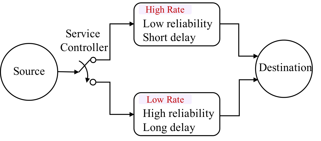
Refer to caption
Figure 1. Model

We consider a status update system, in which update packets are sent to the destination via a wireless medium with varying transmission delay and error probability. The update packets are generated whenever the wireless medium becomes idle. We assume that there are two heterogenous transmissions available for updating, namely low rate and high rate transmissions. The high rate transmission offers a shorter transmission delay than low rate transmission; while low rate transmission offers more reliable transmission than high rate transmission. A decision maker chooses a transmission rate for each transmission opportunity. We denote the set of transmission rates as 𝒰≜{1,2}\mathcal{U}\triangleq\{1,2\}, where 1 and 2 denote the low rate and high rate transmissions, respectively. We use 𝒫≜{pj:0<pj<1,j∈𝒰}\mathcal{P}\triangleq\{p_{j}:0<p_{j}<1,j\in\mathcal{U}\} and 𝒟≜{dj:0<dj<∞,j∈𝒰}\mathcal{D}\triangleq\{d_{j}:0<d_{j}<\infty,j\in\mathcal{U}\} to denote the set of transmission error probabilities and transmission delays, respectively. Transmission j∈𝒰j\in\mathcal{U} corresponds to transmission delay djd_{j} and transmission error probability pjp_{j}. We assume that d1>d2d_{1}>d_{2} and p1<p2p_{1}<p_{2}.

We use YiY_{i} to denote the transmission delay of packet ii, where Yi∈𝒟Y_{i}\in\mathcal{D}. Let DiD_{i} denote the delivery time of packet ii. Since updates are generated whenever the wireless medium becomes idle, DiD_{i} equals to the generation time of packet i+1i+1. Also, we have Di=∑j=1iYjD_{i}=\sum_{j=1}^{i}Y_{j}.

Refer to caption
Figure 2. Example of Age Evolution

At any time tt, the most recently received update packet is generated at time

(1) U⁡(t)=max⁡{Di:Di+1≤t}.U(t)=\max\{D_{i}:D_{i+1}\leq t\}.

Then, the age of information, or simply age is defined as

(2) Δ⁡(t)=t−U⁡(t).\Delta(t)=t-U(t).

The age Δ⁡(t)\Delta(t) is a stochastic process that increases with tt between update packets and is reset to a smaller value upon the successful delivery of a fresher packet. We suppose that the age Δ⁡(t)\Delta(t) is right-continuous. As shown in Fig. 2, packet 22 is sent at time D1D_{1} and its delivery time is D2=D1+Y2D_{2}=D_{1}+Y_{2}. Since this packet transmission fails, the age does not reset to a smaller value at D2D_{2}. Packet 33 transmission starts at D2D_{2}, which is successfully delivered at time D3D_{3}. Thus, the age increases linearly until it reaches to Δ⁡(D3−)=Y1+Y2+Y3\Delta(D_{3}^{-})=Y_{1}+Y_{2}+Y_{3} before packet 33 is successfully sent, and then drops to Δ⁡(D3)=Y3\Delta(D_{3})=Y_{3} at D3D_{3}.

3. Optimization Problem

We use uiu_{i} to denote which transmission rate (low or high) is selected to transmit packet ii, where ui∈𝒰u_{i}\in\mathcal{U}. In particular, if ui=1u_{i}=1 (or ui=2u_{i}=2), then packet ii is transmitted using the low (or high) rate transmission, encounters transmission delay d1d_{1} (or d2d_{2}), and is received successfully with probability 1−p11-p_{1} (or 1−p21-p_{2}). A transmission selection policy π\pi specifies a transmission selection decision for each stage11 1 Stage ii corresponds to the duration from Di−1D_{i-1} to DiD_{i}.. For any policy π\pi, we define the total average age as

(3) Δ¯​(π)=lim supn→∞𝔼⁡[∫0DnΔ⁡(t)​𝑑t]𝔼⁡[Dn].\bar{\Delta}(\pi)=\limsup_{n\rightarrow\infty}\frac{\mathbb{E}[\int_{0}^{D_{n}}\Delta(t)dt]}{\mathbb{E}[D_{n}]}.

Our goal is to seek a transmission selection policy that solves the total average age minimization problem as follows:

(4) Δ¯∗=minπ∈Π⁡Δ¯​(π),\displaystyle\bar{\Delta}^{*}=\min_{\pi\in\Pi}\bar{\Delta}(\pi),

where Δ¯∗\bar{\Delta}^{*} denotes the optimal total average age. Let Π\Pi denote the set of all causal transmission selection policies, in which the policy π∈Π\pi\in\Pi depends on the history and current system state.

3.1. Equivalent Mapping of Problem (4)

We decompose the area under the curve Δ⁡(t)\Delta(t) into a sum of disjoint geometric parts as shown in Fig. 2. Observing the area in interval [0,Dn][0,D_{n}], the area can be regarded as the concatenation of the areas QiQ_{i}. Then,

(5) ∫0DnΔ⁡(t)​𝑑t=∑i=0n−1[Qi].\displaystyle\int_{0}^{D_{n}}\Delta(t)dt=\sum_{i=0}^{n-1}[Q_{i}].

Let aia_{i} denote the age at time DiD_{i}, i.e., ai=Δ⁡(Di)a_{i}=\Delta(D_{i}). Then, QiQ_{i} can be expressed as

(6) Qi=ai​Yi+1+12​Yi+12.\displaystyle Q_{i}=a_{i}Y_{i+1}+\frac{1}{2}Y_{i+1}^{2}.

Recall that Dn=∑i=0n−1Yi+1D_{n}=\sum_{i=0}^{n-1}Y_{i+1}. With Eq. (6) and Eq. (5), the total average age is expressed as

(7) lim supn→∞∑0n−1𝔼⁡[ai​Yi+1+12​Yi+12]∑i=0n−1𝔼⁡[Yi+1]..\displaystyle\limsup_{n\rightarrow\infty}\frac{\sum_{0}^{n-1}\mathbb{E}[a_{i}Y_{i+1}+\frac{1}{2}Y_{i+1}^{2}]}{\sum_{i=0}^{n-1}\mathbb{E}[Y_{i+1}]}..

With this, the optimal transmission selection problem for minimizing the total average age can be formulated as

(8) Δ¯∗≜min⁡lim supn→∞π∈Π⁡∑0n−1𝔼⁡[ai​Yi+1+12​Yi+12]∑i=0n−1𝔼⁡[Yi+1].\displaystyle\bar{\Delta}^{*}\triangleq\min_{\pi\in\Pi}\limsup_{n\rightarrow\infty}\frac{\sum_{0}^{n-1}\mathbb{E}[a_{i}Y_{i+1}+\frac{1}{2}Y_{i+1}^{2}]}{\sum_{i=0}^{n-1}\mathbb{E}[Y_{i+1}]}.

The problem is hard to solve in current form. Thus, we provide an equivalent mapping for it. A problem with parameter β\beta is defined as follows:

(9) p⁡(β)≜min⁡lim supn→∞π∈Π⁡1n​∑0n−1𝔼⁡[(ai−β)​Yi+1+12​Yi+12].\displaystyle p(\beta)\triangleq\min_{\pi\in\Pi}\limsup_{n\rightarrow\infty}\frac{1}{n}\sum_{0}^{n-1}\mathbb{E}[(a_{i}-\beta)Y_{i+1}+\frac{1}{2}Y_{i+1}^{2}].
Lemma 3.1.

The following statements are true:

(i) Δ¯∗⪌β\bar{\Delta}^{*}\gtreqqless\beta if and only if p⁡(β)⪌0p(\beta)\gtreqqless 0;

(ii) If p⁡(β)=0p(\beta)=0, then the optimal transmission selection policies that solve (8) and (9) are identical.

Proof.

See Appendix A. ∎

By Lemma 3.1, if β=Δ¯∗\beta=\bar{\Delta}^{*}, then the optimal transmission selection policies that solve (8) and (9) are identical. With this, given β\beta, we formulate the problem (9) as an infinite horizon average cost per stage MDP in Section 3.2 and show that the optimal policy for (9) is of threshold-type in Section 4.1. Since the value of β\beta is arbitrary, we will be able to conclude that the optimal policy for (8) is of threshold-type. In addition, in Section 4.2, we are able to devise a low-complexity algorithm to obtain the optimal threshold.

3.2. The MDP problem of (9)

From (bertsekas1995dynamic), given β\beta, Problem (9) is equivalent to an average cost per stage MDP problem. The components of the MDP problem are described as follows:

  • •

    States: The system state at stage ii is the age aia_{i}. In this paper, we consider the state space 𝒮≜{a=ld1+vd2:l,v∈{0,1,⋯}}\mathcal{S}\triangleq\{a=ld_{1}+vd_{2}:l,v\in\{0,1,\cdots\}\}. If the initial state is outside 𝒮\mathcal{S}, then eventually the state will enter 𝒮\mathcal{S} (with state d1d_{1} or d2d_{2}); otherwise, a successful packet transmission never occurs. In fact, the maximal probability that no transmission succeeds after ll stages is p2lp_{2}^{l}, which decreases with number of stages ll. After state enters 𝒮\mathcal{S}, it will stay in 𝒮\mathcal{S} onwards (since transmission delay is either d1d_{1} or d2d_{2}). Note that 𝒮\mathcal{S} is unbounded since successful packet transmission happens with certain probabilities.

  • •

    Actions: At delivery time Di−1D_{i-1}, the action that is chosen for stage ii is ui∈𝒰u_{i}\in\mathcal{U}. The action uiu_{i} determines the transmission delay. For example, if ui=1u_{i}=1, then the transmission delay at stage ii is d1d_{1}.

  • •

    Transition probabilities: Given the current state aia_{i} and action uiu_{i} at stage ii, the transition probability to the state ai+1a_{i+1} at the stage i+1i+1 is defined as

    (10) P⁡(ai+1=a′|ai=a,ui=u)={puif​a′=a+du,1−puif​a′=du,0otherwise.\displaystyle P(a_{i+1}=a^{\prime}|a_{i}=a,u_{i}=u)=\begin{cases}p_{u}&\text{if}\,\,a^{\prime}=a+d_{u},\\ 1-p_{u}&\text{if}\,\,a^{\prime}=d_{u},\\ 0&\text{otherwise}.\end{cases}
  • •

    Costs: Given state aia_{i} and action uiu_{i} at stage ii, the cost at the stage is defined as

    (11) C⁡(ai,ui)=(ai−β)​dui+12​dui2.\displaystyle C(a_{i},u_{i})=(a_{i}-\beta)d_{u_{i}}+\frac{1}{2}d_{u_{i}}^{2}.

Given β\beta, the average cost per stage under a transmission selection policy π\pi is given by

(12) J⁡(π,β)≜lim supn→∞1n​𝔼π​[∑i=0n−1C⁡(ai,ui)].\displaystyle J(\pi,\beta)\triangleq\limsup_{n\rightarrow\infty}\frac{1}{n}\mathbb{E_{\pi}}\left[\sum_{i=0}^{n-1}C(a_{i},u_{i})\right].

Our objective is to find a transmission selection policy π∈Π\pi\in\Pi that minimizes the average cost per stage, which can be formulated as

Problem 1 (Average cost MDP)

(13) minπ∈Π⁡J⁡(π,β).\displaystyle\min_{\pi\in\Pi}J(\pi,\beta).

We say that a transmission selection policy π\pi is average-optimal if it solves the problem in (13). Our goal is to find the average-optimal policy. A transmission selection policy is a sequence of decision rules, i.e., π=(ζ1,ζ2,⋯)\pi=(\zeta_{1},\zeta_{2},\cdots), where a decision rule ζi\zeta_{i} maps the history of states and actions, and the current state to an action. A transmission selection policy is called a stationary deterministic policy if ui=ζ⁡(ai)u_{i}\!=\!\zeta(a_{i}) for all i∈ℕi\in\mathbb{N}, where ζ:𝒮→𝒰\zeta:\!\mathcal{S}\!\rightarrow\mathcal{U} is a deterministic function. Stationary deterministic policies are the easiest to be implemented and evaluated. However, there may not exist a stationary deterministic policy that is average-optimal (bertsekas1995dynamic). Next, we show that there exists a stationary deterministic transmission selection policy that is average-optimal. Moreover, we show that the optimal policy is of a threshold-type.

4. Structure of Average-Optimal Policy and Algorithm Design

In this section, we investigate the structure of average-optimal policy that minimizes the average cost in (12) and propose an efficient algorithm.

4.1. Threshold Structure of Average-Optimal Policy

4.1.1. Threshold structure:

The following theorem states that there exists a threshold-type stationary deterministic policy that is average-optimal. In particular, the problem is divided into two cases based on the relation between d1​(1−p2)d_{1}(1-p_{2}) and d2​(1−p1)d_{2}(1-p_{1}). Under these two cases, the threshold-type average-optimal policy shows opposite behaviors.

Theorem 4.1.

There exists a stationary deterministic average-optimal transmission selection policy that is of threshold-type. Specifically,

(i) If d1​(1−p2)≤d2​(1−p1)d_{1}(1-p_{2})\leq d_{2}(1-p_{1}), then (12) can be minimized by the policy of the form π∗=(ζ∗,ζ∗,⋯)\pi^{*}=(\zeta^{*},\zeta^{*},\cdots), where

(14) ζ∗​(a)={2if​  0≤a≤a1∗,1if​a1∗<a,\displaystyle\zeta^{*}(a)=\begin{cases}2&\text{if}\,\,0\leq a\leq a_{1}^{*},\\ 1&\text{if}\,\,a_{1}^{*}<a,\end{cases}

where a1∗a_{1}^{*} denotes the age threshold.

(ii) If d1​(1−p2)≥d2​(1−p1)d_{1}(1-p_{2})\geq d_{2}(1-p_{1}), then (12) can be minimized by the policy of the form π∗=(ζ∗,ζ∗,⋯)\pi^{*}=(\zeta^{*},\zeta^{*},\cdots), where

(15) ζ∗​(a)={1if​  0≤a≤a2∗,2if​a2∗<a,\displaystyle\zeta^{*}(a)=\begin{cases}1&\text{if}\,\,0\leq a\leq a_{2}^{*},\\ 2&\text{if}\,\,a_{2}^{*}<a,\end{cases}

where a2∗a_{2}^{*} denotes the age threshold.

Proof.

Please see Section 4.1.2. ∎

Define the mean delay of transmission j∈ℰj\in\mathcal{E} as

(16) d¯j≜dj1−pj.\displaystyle\bar{d}_{j}\triangleq\frac{d_{j}}{1-p_{j}}.

By Theorem 4.1 (i), when the age exceeds a certain threshold, the optimal policy chooses the transmission with smaller mean delay. This result reveals an interesting phenomenon: While the transmission with minimum mean delay is the optimal decision for minimizing the average delay, this does not necessarily minimize the age. In particular, when the age is below a certain threshold, the average age is reduced by choosing a faster transmission that has a higher mean delay (i.e., a higher error probability). The reason is that if successful, the age remains low. If it fails, it provides an opportunity to generate a later packet that can be transmitted in a shorter period of time. In Section 4.2, based on Theorem 4.1 (ii), we will show that the optimal policy under d1​(1−p2)≥d2​(1−p1)d_{1}(1-p_{2})\geq d_{2}(1-p_{1}) is to choose transmission rate 22 for each transmission opportunity. This is reasonable because both the delay and mean delay (including the impact of the error probability) of transmission rate 22 is shorter than that of transmission rate 11.

4.1.2. Proof of Theorem 4.1

One way to investigate the average cost MDPs is to relate them to the discounted cost MDPs. To prove Theorem 4.1, we (i) address a discounted cost MDP, i.e., establish the existence of a stationary deterministic policy that solves the MDP and then study the structure of the optimal policy; and (ii) extend the results to the average cost MDP in (13).

Given an initial state aa, the total expected α\alpha-discounted cost under a transmission selection policy π∈Π\pi\in\Pi is given by

(17) Vα​(a,π)=lim supn→∞𝔼⁡[∑i=0n−1αi​C​(ai,ui)],\displaystyle V^{\alpha}(a;\pi)=\limsup_{n\rightarrow\infty}\mathbb{E}\left[\sum_{i=0}^{n-1}\alpha^{i}C(a_{i},u_{i})\right],

where 0<α<10<\alpha<1 is the discount factor. Then, the optimization problem of minimizing the total expected α\alpha-discounted cost can be cast as

Problem 2 (Discounted cost MDP)

(18) Vα​(a)≜minπ⁡Vα​(a,π),\displaystyle V^{\alpha}(a)\triangleq\min_{\pi}V^{\alpha}(a;\pi),

where Vα​(a)V^{\alpha}(a) denotes the optimal total expected α\alpha-discounted cost. A transmission selection policy is said to be α\alpha-discounted cost optimal if it solves the problem in (18). In Proposition 4.2, we show that there exists a stationary deterministic transmission selection policy which is α\alpha-discounted cost optimal and provide a way to explore the property of the optimal policy.

Proposition 4.2.

(a) The optimal total expected α\alpha-discounted cost VαV^{\alpha} satisfies the following optimality equation:

(19) Vα​(a)=minu∈𝒰⁡Qα​(a,u),\displaystyle V^{\alpha}(a)=\min_{u\in\mathcal{U}}Q^{\alpha}(a,u),

where

(20) Qα​(a,u)=C⁡(a,u)+α​pu​Vα​(a+du)+α⁡(1−pu)​Vα​(du).\displaystyle Q^{\alpha}(a,u)=C(a,u)+\alpha p_{u}V^{\alpha}(a+d_{u})+\alpha(1-p_{u})V^{\alpha}(d_{u}).

(b) The stationary deterministic policy determined by the right-hand-side of (19) is α\alpha-discounted cost optimal.

(c) Let Vnα​(a)V_{n}^{\alpha}(a) be the cost-to-go function such that V0α​(a)=d1−d2α⁡(p2−p1)​aV_{0}^{\alpha}(a)=\frac{d_{1}-d_{2}}{\alpha(p_{2}-p_{1})}a and for n≥0n\geq 0

(21) Vn+1α​(a)=minu∈ℰ⁡Qn+1α​(a,u),\displaystyle V_{n+1}^{\alpha}(a)=\min_{u\in\mathcal{E}}Q_{n+1}^{\alpha}(a,u),

where

(22) Qn+1α​(a,u)=C⁡(a,u)+α​pu​Vnα​(a+du)+α⁡(1−pu)​Vnα​(du).\displaystyle Q_{n+1}^{\alpha}(a,u)=C(a,u)+\alpha p_{u}V_{n}^{\alpha}(a+d_{u})+\alpha(1-p_{u})V_{n}^{\alpha}(d_{u}).

Then, we have that for each α\alpha, Vnα​(a)→Vα​(a)V_{n}^{\alpha}(a)\rightarrow V^{\alpha}(a) as n→∞n\rightarrow\infty.

Proof.

See Appendix B. ∎

Next, with the optimality equation (19) and value iteration (21), we show that the optimal policy is of threshold-type in Lemma 4.3.

Lemma 4.3.

Given a discount factor α\alpha,

(i) if (1−α​p2)​d1≤(1−α​p1)​d2(1-\alpha p_{2})d_{1}\leq(1-\alpha p_{1})d_{2}, then the α\alpha-discounted cost optimal policy is of threshold-type, i.e., the optimal decision is non-increasing in age.

(ii) if (1−α​p2)​d1≥(1−α​p1)​d2(1-\alpha p_{2})d_{1}\geq(1-\alpha p_{1})d_{2}, then the α\alpha-discounted cost optimal policy is of threshold-type, i.e., the optimal decision is non-decreasing in age.

Proof.

Please see Appendix C ∎

This lemma proves that the α\alpha-discounted cost optimal policy is of threshold type. Next, we extend the results to average cost MDP and show that there exists a stationary deterministic average-optimal policy which is of threshold-type. Based on the results in (sennott1989average), we have the following lemma, which provides a candidate for average-optimal policy.

Lemma 4.4.

(i) Let αn\alpha_{n} be any sequence of discount factors converging to 1 with αn\alpha_{n}-discounted cost optimal stationary deterministic policy παn\pi^{\alpha_{n}}. There exists a subsequence γn\gamma_{n} and a stationary policy π⋆\pi^{\star} that is a limit point of πγn\pi^{\gamma_{n}}.

(ii) If d1​(1−p2)≤d2​(1−p1)d_{1}(1-p_{2})\leq d_{2}(1-p_{1}), π⋆\pi^{\star} is of threshold-type in (14); if d1​(1−p2)≥d2​(1−p1)d_{1}(1-p_{2})\geq d_{2}(1-p_{1}), π⋆\pi^{\star} is of threshold-type in (15).

Proof.

See Appendix D. ∎

By (sennott1989average), under certain conditions (A proof of these conditions verification is provided in Appendix E), π⋆\pi^{\star} is average-optimal.

4.2. Algorithm Design

Recall that if p⁡(β)=0p(\beta)=0, then the optimal transmission selection policies that solve (8) and (9) are identical. Given β\beta, the optimal policy that solves (9) is of threshold-type by Theorem 4.1 and then (9) can be re-expressed as

(23) p⁡(β)≜\displaystyle p(\beta)\triangleq minπ∈Π1⁡J⁡(π,β),\displaystyle\min_{\pi\in\Pi_{1}}J(\pi,\beta), if d1​(1−p2)<d2​(1−p1)d_{1}(1-p_{2})<d_{2}(1-p_{1})
(24) p⁡(β)≜\displaystyle p(\beta)\triangleq minπ∈Π2⁡J⁡(π,β),\displaystyle\min_{\pi\in\Pi_{2}}J(\pi,\beta), if d1​(1−p2)≥d2​(1−p1)d_{1}(1-p_{2})\geq d_{2}(1-p_{1})

where Π1\Pi_{1} and Π2\Pi_{2} denote the sets of threshold-type policies in (14) and (15), respectively. Thus, the optimal policy that solves (8) can be obtained with two steps:

  • •

    Step (i): For each β\beta, find the β\beta-associated optimal policy πβ∗\pi^{*}_{\beta} such that p⁡(β)=J⁡(πβ∗,β)p(\beta)=J(\pi^{*}_{\beta},\beta).

  • •

    Step (ii): Find β∗\beta^{*} such that p⁡(β∗)=0p(\beta^{*})=0. This implies πβ∗∗\pi^{*}_{\beta^{*}} solves (8).

To narrow our searching range in (ii), in Lemma 4.5, we provide a lower bound βmin\beta_{\text{min}} and an upper bound βmax\beta_{\text{max}} of β∗\beta^{*}. Then, for (i), we only need to pay attention to p⁡(β)p(\beta) for β∈[βmin,βmax]\beta\in[\beta_{\text{min}},\beta_{\text{max}}].

In particular, within the range of β\beta, we show that JJ in (23) is quasi-convex in a threshold related variable, which enables us to devise a low-complexity algorithm based on golden section search. Moreover, we show that πβ∗\pi^{*}_{\beta} that solves (24) always chooses u=2u=2, which allows us to get the optimal policy for (8) directly.

Lemma 4.5.

The parameter β∗\beta^{*} is lower bounded by βmin≜1.5​d2\beta_{\text{min}}\triangleq 1.5d_{2} and upper bounded by βmax≜min⁡{(11−p1+0.5)​d1,(11−p2+0.5)​d2}\beta_{\text{max}}\triangleq\min\Big\{(\frac{1}{1-p_{1}}+0.5)d_{1},(\frac{1}{1-p_{2}}+0.5)d_{2}\Big\}.

Proof.

See Appendix F. ∎

In the following content, we provide a theoretical analysis step by step for our algorithm design in Algorithm 1, which returns the optimal threshold and optimal average age.

given d1d_{1}, d2d_{2}, p1p_{1}, p2p_{2},τ=(5−1)/2\tau=(\sqrt{5}-1)/2, tolerance ϵ1\epsilon_{1}, ϵ2\epsilon_{2}, l=βminl=\beta_{\text{min}}, r=βmaxr=\beta_{\text{max}}; 1
while r−l>ϵ1r-l>\epsilon_{1} do 2
β=r+l2\beta=\frac{r+l}{2}; 3
      if d1​(1−p2)≥d2​(1−p1)d_{1}(1-p_{2})\geq d_{2}(1-p_{1}) then 4
      m=0m=0, k=0k=0, J∗=J2​(0,0,β)J^{*}=J_{2}(0,0,\beta); 5
          else 6
      kmax=⌊d1d2⌋k_{\text{max}}=\lfloor\frac{d_{1}}{d_{2}}\rfloor, J∗=f⁡(1,0,β)J^{*}=f(1,0,\beta); 7
           foreach k1∈{0,1,⋯,kmax}k_{1}\in\{0,1,\cdots,k_{\text{max}}\} do 8
           if ∂J1​(y,k1,β)∂y|y=1<0\frac{\partial J_{1}(y,k_{1},\beta)}{\partial y}|_{y=1}<0 then 9
                m=0m=0; 10
                     else 11
                y0=0y_{0}=0, y1=1y_{1}=1, y2=y1−(y1−y0)​τy_{2}=y_{1}-(y_{1}-y_{0})\tau, y3=y0+(y1−y0)​τy_{3}=y_{0}+(y_{1}-y_{0})\tau; 12
                     while p2​y1≥y0p_{2}y_{1}\geq y_{0} and y1−y0>ϵ2y_{1}-y_{0}>\epsilon_{2} do 13
                     if J1​(y2,k1,β)>J1​(y3,k1,β)J_{1}(y_{2},k_{1},\beta)>J_{1}(y_{3},k_{1},\beta) then 14
                          y0=y2y_{0}=y_{2}; 15
                               else 16
                          y1=y3y_{1}=y_{3}; 17
                               end if 18
                         y2=y1−(y1−y0)​τy_{2}=y_{1}-(y_{1}-y_{0})\tau, y3=y0+(y1−y0)​τy_{3}=y_{0}+(y_{1}-y_{0})\tau; 19
                          end while 20
                    t1=⌊logp2⁡y0⌋t_{1}=\lfloor\log_{p_{2}}y_{0}\rfloor, t2=⌈logp2⁡y1⌉t_{2}=\lceil\log_{p_{2}}y_{1}\rceil; 21
                     m=arg​minm∈{t1,t2}⁡J1​(p2m,k,β)m=\argmin_{m\in\{t_{1},t_{2}\}}J_{1}({p_{2}}^{m};k,\beta); 22
                     end if 23
               if J1​(p2m,k1,β)≤J∗J_{1}(p_{2}^{m},k_{1},\beta)\leq J^{*} then 24
                J∗=J1​(p2m,k1,β)J^{*}=J_{1}(p_{2}^{m},k_{1},\beta); 25
                     end if 26
                end foreach 27
           end if 28
     if J∗≥0J^{*}\geq 0 then 29
      l=βl=\beta; 30
          else 31
      r=βr=\beta; 32
           end if 33
      34
      end while 35
Algorithm 1 Threshold-based Age-Optimal Policy

Step (i): Find the optimal policy πβ∗\pi^{*}_{\beta}: Note that both of the threshold-type policies defined in (14) and (15) result in a Markov chain with a single positive recurrent class. Thus, given threshold a1∗a_{1}^{*} in (14) or a2∗a_{2}^{*} in (15), we can obtain the expression of average cost under the corresponding threshold-type policy with aid of state transition diagram. With this, we obtain some nice properties in Theorem 4.6, which enables us to get a low-complexity algorithm. Before providing the result, we define the integer threshold which will be used in the theorem and algorithm.

Recall that age a∈𝒮a\in\mathcal{S} is expressed as the sum of multiple d1d_{1}’s and d2d_{2}’s. Note that under the threshold-type policy in (14), if a<a1∗a<a_{1}^{*}, ζ⁡(a)=2\zeta(a)=2. This implies that if a<a1∗a<a_{1}^{*}, aa is in the form a=dj+l​d2,j∈ℰ,l∈ℕa=d_{j}+ld_{2},j\in\mathcal{E},l\in\mathbb{N}. Thus, it is sufficient to use the following integer threshold to represent the threshold-type policy in (14).

(25) m1\displaystyle m_{1} =min{l:d1+ld2≥a1∗,l∈ℕ},\displaystyle=\min\left\{l:d_{1}+ld_{2}\geq a_{1}^{*},l\in\mathbb{N}\right\},
(26) n1\displaystyle n_{1} =min{l:d2+ld2≥a1∗,l∈ℕ}.\displaystyle=\min\left\{l:d_{2}+ld_{2}\geq a_{1}^{*},l\in\mathbb{N}\right\}.

Similarly, the policy in (15) can be represented by

(27) m2\displaystyle m_{2} =min{l:d1+ld1≥a2∗,l∈ℕ},\displaystyle=\min\left\{l:d_{1}+ld_{1}\geq a_{2}^{*},l\in\mathbb{N}\right\},
(28) n2\displaystyle n_{2} =min{l:d2+ld1≥a2∗,l∈ℕ},.\displaystyle=\min\left\{l:d_{2}+ld_{1}\geq a_{2}^{*},l\in\mathbb{N}\right\},.

Based on the analysis, (23) and (24) can be re-expressed as

(29) p⁡(β)≜\displaystyle p(\beta)\triangleq minm1,k1⁡J1​(m1,k1,β),\displaystyle\min_{m_{1},k_{1}}J_{1}(m_{1},k_{1},\beta), ​if d1​(1−p2)<d2​(1−p1)d_{1}(1-p_{2})\!\!<\!d_{2}(\!1-p_{1}\!)
(30) p⁡(β)≜\displaystyle p(\beta)\triangleq minm2,k2⁡J2​(m2,k2,β),\displaystyle\min_{m_{2},k_{2}}J_{2}(m_{2},k_{2},\beta), ​if d1​(1−p2)≥d2​(1−p1)d_{1}(1-p_{2})\!\!\geq\!d_{2}(\!1-p_{1}\!)

where k1=n1−m1k_{1}=n_{1}-m_{1} and k2=n2−m2k_{2}=n_{2}-m_{2}. Also, we use J1​(m1,k1,β)J_{1}(m_{1},k_{1},\beta) and J2​(m2,k2,β)J_{2}(m_{2},k_{2},\beta) to denote the average cost under the policies in (14) and (15), respectively. We have k2∈𝒦2≜{0,1}k_{2}\in\mathcal{K}_{2}\triangleq\{0,1\} and k1∈𝒦1≜{0,⋯,⌊d1d2⌋}k_{1}\in\mathcal{K}_{1}\triangleq\big\{0,\cdots,\lfloor\frac{d_{1}}{d_{2}}\rfloor\big\}. In particular, according to the definition of m2m_{2} and n2n_{2}, we have (m2+1)​d1≥a2∗>d2+(n2−1)​d1(m_{2}+1)d_{1}\geq a_{2}^{*}>d_{2}+(n_{2}-1)d_{1} and d2+n2​d1≥a2∗>m2​d1d_{2}+n_{2}d_{1}\geq a_{2}^{*}>m_{2}d_{1}. Substitute k2=n2−m2k_{2}=n_{2}-m_{2} into these two inequalities, we get k2∈𝒦2k_{2}\in\mathcal{K}_{2}. Similarly, we have k1∈𝒦1k_{1}\in\mathcal{K}_{1}.

Table 1. Notations
A1A_{1} =p2k1​(d2​(1−p1)−d1​(1−p2))​(d2​(k1+1)−d1)=p_{2}^{k_{1}}\big(d_{2}(1-p_{1})-d_{1}(1-p_{2})\big)\big(d_{2}(k_{1}+1)-d_{1}\big)
B1B_{1} =−A2+p2k1​(1−p2)​(0.5​d12−β​d1+d121−p1)+(1−p1)​(β​d2−0.5​d22−d221−p2)=-A_{2}+p_{2}^{k_{1}}(1-p_{2})(0.5d_{1}^{2}-\beta d_{1}+\frac{d_{1}^{2}}{1-p_{1}})+(1-p_{1})(\beta d_{2}-0.5d_{2}^{2}-\frac{d_{2}^{2}}{1-p_{2}})
C1C_{1} =(1−p1)​(0.5​d22−β​d2+11−p2)​d22=(1-p_{1})(0.5d_{2}^{2}-\beta d_{2}+\frac{1}{1-p_{2}})d_{2}^{2}
D1D_{1} =(d1​(1−p2)−d2​(1−p1))​d2​p2k1=\big(d_{1}(1-p_{2})-d_{2}(1-p_{1})\big)d_{2}p_{2}^{k_{1}}
A2A_{2} =p1k2​(d1​(1−p2)−d2​(1−p1))​(d1​(1−k2)−d2)=p_{1}^{k_{2}}\big(d_{1}(1-p_{2})-d_{2}(1-p_{1})\big)\big(d_{1}(1-{k_{2}})-d_{2}\big)
B2B_{2} =−p1k2​(1−p2)​(0.5​d12−β​d1+d121−p1)+(1−p1)​(0.5​d22−β​d2+d221−p2)=-p_{1}^{k_{2}}(1-p_{2})(0.5d_{1}^{2}-\beta d_{1}+\frac{d_{1}^{2}}{1-p_{1}})+(1-p_{1})(0.5d_{2}^{2}-\beta d_{2}+\frac{d_{2}^{2}}{1-p_{2}})
−(d1​(1−p2)−d2​(1−p1))​(d1−d2)\ \ \ \ -\big(d_{1}(1-p_{2})-d_{2}(1-p_{1})\big)(d_{1}-d_{2})
C2C_{2} =(1−p2)​(0.5​d12−β​d1+d121−p1)=(1-p_{2})(0.5d_{1}^{2}-\beta d_{1}+\frac{d_{1}^{2}}{1-p_{1}})
D2D_{2} =(d2​(1−p1)−d1​(1−p2))​d1=\big(d_{2}(1-p_{1})-d_{1}(1-p_{2})\big)d_{1}

In Theorem 4.6, we provide some nice properties for J1J_{1} and J2J_{2}, which enables us to develop a low-complexity algorithm. Some notations used in this theorem are defined in Table 1.

Theorem 4.6.

Given β∈[βmin,βmax]\beta\in[\beta_{\text{min}},\beta_{\text{max}}],

(i) if d1​(1−p2)<d2​(1−p1)d_{1}(1-p_{2})<d_{2}(1-p_{1}), then the average cost under the policy in (14) is given by

(31) J1​(y,k1,β)=A1​y2+B1​y+C1+D1​y​logp2⁡(y)1−p1+(−1+p1+p2k1​(1−p2))​y,J_{1}(y,k_{1},\beta)=\frac{A_{1}y^{2}+B_{1}y+C_{1}+D_{1}y\log_{p_{2}}(y)}{1-p_{1}+(-1+p_{1}+p_{2}^{k_{1}}(1-p_{2}))y},

where y≜p2m1y\triangleq p_{2}^{m_{1}}. Moreover, J1​(y,k1,β)J_{1}(y,k_{1},\beta) is quasi-convex in yy for 0<y≤10<y\leq 1, given k1∈𝒦1k_{1}\in\mathcal{K}_{1}.

(ii) if d1​(1−p2)≥d2​(1−p1)d_{1}(1-p_{2})\geq d_{2}(1-p_{1}), then optimal average cost is given by

(32) J2​(0,0,β)=A2+B2+C21−p1.J_{2}(0,0,\beta)=\frac{A_{2}+B_{2}+C_{2}}{1-p_{1}}.

Moreover, the optimal policy for (30) chooses u=2u=2 at every transmission opportunity.

Proof.

See Appendix G. ∎

With the property in Theorem 4.6 (i), we are able to use golden section search (press2007section) to find the optimal value of yy under condition d1​(1−p2)<d2​(1−p1)d_{1}(1-p_{2})<d_{2}(1-p_{1}). The details are provided in Algorithm 1 (Line 12-20). In Theorem 4.6 (i), we make a change of variable, i.e., m1m_{1} is replaced with logp2⁡(y)\log_{p_{2}}(y) in J1J_{1}, where y∈(0,1]y\in(0,1]. Note that logp2⁡(⋅)\log_{p_{2}}(\cdot) is one-to-one functions. Thus, after obtaining the optimal yy that minimizes J1J_{1} , the corresponding optimal threshold m1m_{1} can be easily obtained by comparing J1​(p2⌊logp2⁡(y)⌋,k1,β)J_{1}({p_{2}}^{\lfloor\log_{p_{2}}(y)\rfloor},k_{1},\beta) and J1​(p2⌈logp2⁡(y)⌉,k1,β)J_{1}({p_{2}}^{\lceil\log_{p_{2}}(y)\rceil};k_{1},\beta)). The details are provided in Algorithm 1 (Line 21-22). Till now, we have solved minm1⁡J1​(m1,k1,β)\min_{m_{1}}J_{1}(m_{1},k_{1},\beta) given k1k_{1} and β\beta. Note that k1∈𝒦1k_{1}\in\mathcal{K}_{1} has finite and countable values. Then, we can easily solve (29) under condition d1​(1−p2)<d2​(1−p1)d_{1}(1-p_{2})<d_{2}(1-p_{1}) by searching for the optimal k1k_{1} in the finite set 𝒦1\mathcal{K}_{1}.

Note that Theorem 4.6 (ii) applies to all β∈[βmin,βmax]\beta\in\![\beta_{\text{min}},\!\beta_{\text{max}}\!] including β∗\beta^{*}. Thus, the optimal policy for (15) is to take u=2u=2 at every transmission opportunity, which is returned directly in Algorithm 1 (Line 4-5). Under this condition, the step (ii) is only used to find optimal average cost β∗\beta^{*}.

Moreover, in Line 9-10, we add a judgement sentence, i.e., if the condition ∂J1​(y,k1,β)∂y|y=1<0\frac{\partial J_{1}(y,k_{1},\beta)}{\partial y}|_{y=1}<0 is satisfied, then we can directly obtain the optimal m1m_{1} without running golden section method. This further reduces the algorithm complexity. The judgement is based on the fact that limy→0∂J1​(y,k1,β)∂y<0\lim_{y\rightarrow 0}\frac{\partial J_{1}(y,k_{1},\beta)}{\partial y}<0 (this is proved in the proof of Theorem 4.6 in Appendix G) and J1J_{1} is quasi-convex. Thus, if ∂J1​(y,k1,β)∂y|y=1<0\frac{\partial J_{1}(y,k_{1},\beta)}{\partial y}|_{y=1}<0, then J1J_{1} is non-increasing in yy.

Step (ii): Find β∗\beta^{*}: By Lemma 3.1, if p⁡(β)>0p(\beta)>0, then β<β∗\beta<\beta^{*}; if p⁡(β)<0p(\beta)<0, then β>β∗\beta>\beta^{*}. Thus, we can use bisection method to search for β∗\beta^{*}. The details are provided in Algorithm 1 (Line 2-3 and Line 29-33).

5. A Discussion on the General Multi-Rate Transmission Selection Problem

For the multi-rate transmission selection (from more than two-rate) problem, we assume that there are N∈ℕ+N\in\mathbb{N}^{+} transmissions for selection such that transmission delays and error probabilities satisfy dj>dj+1d_{j}>d_{j+1} and pj<pj+1p_{j}<p_{j+1}, for j∈{1,2,⋯,N}j\in\{1,2,\cdots,N\}, respectively. Since the transmission delays and transmission error probabilities affect the age in opposite direction, it may be difficult to determine the optimal policy. Thanks to the results obtained for the two-rate transmission selection problem, we obtain some useful insights for the general multi-rate transmission selection.

In particular, for the two-rate transmission selection problem, the optimal decision is monotonically non-increasing in age under condition d¯1≤d¯2\bar{d}_{1}\leq\bar{d}_{2} and monotonically non-decreasing in age under condition d¯1≥d¯2\bar{d}_{1}\geq\bar{d}_{2}, where d¯1\bar{d}_{1} and d¯2\bar{d}_{2} are mean delays of low and high rate transmissions, respectively, as defined in (16). The monotonic property is obtained by showing that Q function Qα​(a,u)Q^{\alpha}(a,u) in (20) is supermodular (submodular) in (a,u)(a,u) under former (later) condition. If we apply the same technique to the multi-rate transmission selection, we will be able to get the following properties:

  • •

    (i) if d¯1≤d¯2≤⋯≤d¯N\bar{d}_{1}\leq\bar{d}_{2}\leq\cdots\leq\bar{d}_{N}, then the optimal decision will be monotonically non-increasing in age,

  • •

    (ii) if d¯1≥d¯2≥⋯≥d¯N\bar{d}_{1}\geq\bar{d}_{2}\geq\cdots\geq\bar{d}_{N}, then the optimal decision will be monotonically non-decreasing in age.

Specifically, for (i), to show the monotonic property, we can show that given transmission l∈{1,2,⋯,N}l\in\{1,2,\cdots,N\}, any transmission vv with longer delay, i.e. dv>dld_{v}>d_{l}, satisfy that Q function is supermodular in (a,u)(a,u). Since the state space is not changed, it will be provable with this technique. The same analysis applies to (ii). However, for the cases that are not covered in (i) and (ii), we need more investigation on the property of the optimal policy and may use other techniques for the proof, which is for our future work.

In addition, if we can show that the optimal policy for the general multi-rate problem is of threshold-type, then machine learning algorithms can be used to determine the optimal threshold. For example, if we regard each threshold-type policy with a certain threshold as a bandit, then basic bandit algorithms like UCB can be exploited to find the optimal threshold (prabuchandran2016reinforcement).

6. Numerical Results

In this section, we present some numerical results to explore the performance of the threshold-based age-optimal policy and verify our theoretical results.

First, we consider an update system, in which p1=0.4p_{1}=0.4 and p2=0.75p_{2}=0.75. Table. 2 illustrates the relation between the optimal threshold versus the transmission delay d2d_{2} and the delay ratio d1d2\frac{d_{1}}{d_{2}} under condition d2​(1−p1)>d1​(1−p2)d_{2}(1-p_{1})>d_{1}(1-p_{2}). The threshold (m1,n1)(m_{1},n_{1}) in the table is obtained by Algorithm 1. We observe that the threshold increases with either d2d_{2} or the delay ratio d1d2\frac{d_{1}}{d_{2}}. Note that when the age is below the threshold, transmission rate 22 is selected. Thus, this observation implies that transmission rate 22 becomes more preferable either when d2d_{2} increases with fixed d1d2\frac{d_{1}}{d_{2}} or when d1d2\frac{d_{1}}{d_{2}} increases with fixed d2d_{2}.

Table 2. Optimal threshold versus delay
d1=1.5​d2d_{1}\!\!=\!\!1.5d_{2} d1=1.7​d2d_{1}\!\!=\!\!1.7d_{2} d1=1.9​d2d_{1}\!\!=\!\!1.9d_{2} d1=2.1​d2d_{1}\!\!=\!\!2.1d_{2} d1=2.3​d2d_{1}\!\!=\!\!2.3d_{2}
d2=1d_{2}\!\!=\!\!1 (0,0) (0,0) (1,2) (3,4) (15,16)
d2=5d_{2}\!\!=\!\!5 (0,1) (0,1) (1,2) (3,4) (15,16)
d2=9d_{2}\!\!=\!\!9 (0,1) (0,1) (1,2) (3,4) (15,16)

In Fig. 3, we consider an update system, in which the transmission delays are d1=10d_{1}=10 and d2=8d_{2}=8. We use “Delay-Optimal” to denote the optimal policy that minimizes the average delay by always choosing the transmission rate with minimum mean delay (ozkan2014optimal; de2005managing). Moreover, we use “Age-Optimal” to denote the optimal policy that is obtained from Algorithm 1. We use “Random pp” to denote the policy that chooses transmission rate 11 with probability pp. We compare our threshold-based “Age-Optimal” policy with “Random pp” policies and the “Delay-Optimal” policy, where p∈{0.25,0.5}p\in\{0.25,0.5\}.

(a) Average age vs p1p_{1} given p2=0.5p_{2}=0.5
(b) Average age vs p2p_{2} given p1=0.5p_{1}=0.5
Figure 3. Total average age versus transmission error probability

Fig. 3a (3b) illustrates the total average age in (7) versus transmission error probability p1p_{1} (p2p_{2}) given p2=0.5p_{2}=0.5 (p1=0.5p_{1}=0.5). The dashed line in the figure marks the point at which d1​(1−p2)=d2​(1−p1)d_{1}(1-p_{2})=d_{2}(1-p_{1}). The left and right (right and left) of the line corresponds to conditions d1​(1−p2)<d2​(1−p1)d_{1}(1-p_{2})<d_{2}(1-p_{1}) and d1​(1−p2)>d2​(1−p1)d_{1}(1-p_{2})>d_{2}(1-p_{1}) in Fig. 3a (in Fig. 3b), respectively. As we can observe, the age-optimal policy outperforms other plotted policies. This agrees with Theorem 4.1. Moreover, the results confirm that the delay-optimal policy does not necessarily minimize the age. In particular, the gap between delay-optimal and age-optimal policy becomes larger as p1p_{1} (p2p_{2}) approaches to the left side (right side) of the dashed line in Fig. 3a (Fig. 3b). The jump in the curve of the delay-optimal policy is incurred by the switch between two transmission rates. For example, in Fig. 3a, delay-optimal policy chooses u=1u=1 on the left side of the dashed line, while chooses u=2u=2 on the right side. This is because transmission rate 11 has smaller mean delay on the left side while transmission rate 22 has smaller mean delay on the right side.

7. Conclusion

In this paper, we studied the transmission selection problem for minimizing age of information in information update system with heterogenous transmissions. We assume that there are two different transmissions with varying delay and error probability. We showed that there exists a stationary deterministic optimal transmission selection policy which is of threshold-type in age (Theorem 4.1). This result reveals an interesting phenomenon: If the mean delay of the low rate transmission is smaller than that of high rate transmission, then the optimal action chooses the one with higher mean delay when age is smaller than a certain threshold. This is in contrary with the delay-optimal policy that always chooses the transmission with lower mean delay. In addition, we showed that if the mean delay of the low rate transmission is smaller than that of high rate transmission, the average cost is quasi-convex in a threshold related variable; otherwise, the optimal policy chooses u=2u=2 for each transmission opportunity (Theorem 4.6). This enabled us to design a low-complexity algorithm to obtain the optimal policy (Algorithm 1). For the future work, we plan to study the multi-rate scenario with more than two selections of heterogenous transmissions based on the insights discussed in Section 5.

References

  • [1] Roy D Yates. Lazy is timely: Status updates by an energy harvesting source. In 2015 IEEE International Symposium on Information Theory (ISIT), pages 3008–3012. IEEE, 2015.
  • [2] Igor Kadota, Abhishek Sinha, Elif Uysal-Biyikoglu, Rahul Singh, and Eytan Modiano. Scheduling policies for minimizing age of information in broadcast wireless networks. IEEE/ACM Transactions on Networking, 26(6):2637–2650, 2018.
  • [3] Ahmed M Bedewy, Yin Sun, Rahul Singh, and Ness B Shroff. Optimizing information freshness using low-power status updates via sleep-wake scheduling. In Proceedings of the Twenty-First International Symposium on Theory, Algorithmic Foundations, and Protocol Design for Mobile Networks and Mobile Computing, pages 51–60, 2020.
  • [4] Sanjit Kaul, Marco Gruteser, Vinuth Rai, and John Kenney. Minimizing age of information in vehicular networks. In 2011 8th Annual IEEE Communications Society Conference on Sensor, Mesh and Ad Hoc Communications and Networks, pages 350–358. IEEE, 2011.
  • [5] Yin Sun, Elif Uysal-Biyikoglu, Roy D Yates, C Emre Koksal, and Ness B Shroff. Update or wait: How to keep your data fresh. IEEE Transactions on Information Theory, 63(11):7492–7508, 2017.
  • [6] Baran Tan Bacinoglu, Elif Tugce Ceran, and Elif Uysal-Biyikoglu. Age of information under energy replenishment constraints. In 2015 Information Theory and Applications Workshop (ITA), pages 25–31. IEEE, 2015.
  • [7] Xianwen Wu, Jing Yang, and Jingxian Wu. Optimal status update for age of information minimization with an energy harvesting source. IEEE Transactions on Green Communications and Networking, 2(1):193–204, 2017.
  • [8] Bo Zhou and Walid Saad. Optimal sampling and updating for minimizing age of information in the internet of things. In 2018 IEEE Global Communications Conference (GLOBECOM), pages 1–6. IEEE, 2018.
  • [9] Elif Tuğçe Ceran, Deniz Gündüz, and András György. Average age of information with hybrid arq under a resource constraint. IEEE Transactions on Wireless Communications, 18(3):1900–1913, 2019.
  • [10] Xu Du, Yin Sun, Ness B Shroff, and Ashutosh Sabharwal. Balancing queueing and retransmission: Latency-optimal massive mimo design. IEEE Transactions on Wireless Communications, 19(4):2293–2307, 2020.
  • [11] Erhun Ozkan and Jeffrey P Kharoufeh. Optimal control of a two-server queueing system with failures. Probability in the Engineering and Informational Sciences, 28(4):489–527, 2014.
  • [12] Francis De Véricourt and Yong-Pin Zhou. Managing response time in a call-routing problem with service failure. Operations Research, 53(6):968–981, 2005.
  • [13] Dimitri P Bertsekas, Dimitri P Bertsekas, Dimitri P Bertsekas, and Dimitri P Bertsekas. Dynamic programming and optimal control, volume 1. Athena scientific Belmont, MA, 1995.
  • [14] Linn I Sennott. Average cost optimal stationary policies in infinite state markov decision processes with unbounded costs. Operations Research, 37(4):626–633, 1989.
  • [15] WH Press, SA Teukolsky, WT Vetterling, and BP Flannery. Section 10.2. golden section search in one dimension. In Numerical recipes: the art of scientific computing, pages 492–496. Cambridge University Press New York, 2007.
  • [16] KJ Prabuchandran, Tejas Bodas, and Theja Tulabandhula. Reinforcement learning algorithms for regret minimization in structured markov decision processes. arXiv preprint arXiv:1608.04929, 2016.
  • [17] Martin L Puterman. Markov decision processes: discrete stochastic dynamic programming. John Wiley & Sons, 2014.
  • [18] Yu-Pin Hsu, Eytan Modiano, and Lingjie Duan. Scheduling algorithms for minimizing age of information in wireless broadcast networks with random arrivals. IEEE Transactions on Mobile Computing, 2019.
  • [19] Stephen Boyd, Stephen P Boyd, and Lieven Vandenberghe. Convex optimization. Cambridge university press, 2004.

Appendix A Proof of Lemma 3.1

We show (i) with two steps.

Step1: This step proves that Δ¯∗≤β\bar{\Delta}^{*}\leq\beta if and only if p⁡(β)≤0p(\beta)\leq 0.

If Δ¯∗≤β\bar{\Delta}^{*}\leq\beta, there exists a π\pi that is feasible for (8) and (9) which satisfies

(33) lim supn→∞∑0n−1𝔼⁡[ai​Yi+1+12​Yi+12]∑i=0n−1𝔼⁡[Yi+1]≤β.\displaystyle\limsup_{n\rightarrow\infty}\frac{\sum_{0}^{n-1}\mathbb{E}[a_{i}Y_{i+1}+\frac{1}{2}Y_{i+1}^{2}]}{\sum_{i=0}^{n-1}\mathbb{E}[Y_{i+1}]}\leq\beta.

Therefore, we have

(34) lim supn→∞1n​∑0n−1𝔼⁡[(ai−β)​Yi+1+12​Yi+12]1n​∑i=0n−1𝔼⁡[Yi+1]≤0.\displaystyle\limsup_{n\rightarrow\infty}\frac{\frac{1}{n}\sum_{0}^{n-1}\mathbb{E}[(a_{i}-\beta)Y_{i+1}+\frac{1}{2}Y_{i+1}^{2}]}{\frac{1}{n}\sum_{i=0}^{n-1}\mathbb{E}[Y_{i+1}]}\leq 0.

Since Yi∈𝒟Y_{i}\in\mathcal{D}, YiY_{i}’s are bounded and positive and 𝔼⁡[Yi]>0\mathbb{E}[Y_{i}]>0 for all ii. Then, we have

0<lim infn→∞1n​∑i=0n−1𝔼⁡[Yi+1]≤lim supn→∞1n​∑i=0n−1𝔼⁡[Yi+1]≤max⁡{d1,d2}.0<\liminf_{n\rightarrow\infty}\frac{1}{n}\sum_{i=0}^{n-1}\mathbb{E}[Y_{i+1}]\leq\limsup_{n\rightarrow\infty}\frac{1}{n}\sum_{i=0}^{n-1}\mathbb{E}[Y_{i+1}]\leq\max\{d_{1},d_{2}\}.

Thus, we obtain

(35) lim supn→∞1n​∑0n−1𝔼⁡[(ai−β)​Yi+1+12​Yi+12]≤0.\displaystyle\limsup_{n\rightarrow\infty}\frac{1}{n}\sum_{0}^{n-1}\mathbb{E}[(a_{i}-\beta)Y_{i+1}+\frac{1}{2}Y_{i+1}^{2}]\leq 0.

That is, p⁡(β)≤0p(\beta)\leq 0. For the reverse direction, if p⁡(β)≤0p(\beta)\leq 0, then there exists a π\pi that is feasible for (8) and (9) which satisfies (35). Since

0<lim infn→∞1n​∑i=0n−1𝔼⁡[Yi+1]≤lim supn→∞1n​∑i=0n−1𝔼⁡[Yi+1]≤max⁡{d1,d2},0<\liminf_{n\rightarrow\infty}\frac{1}{n}\sum_{i=0}^{n-1}\mathbb{E}[Y_{i+1}]\\ \leq\limsup_{n\rightarrow\infty}\frac{1}{n}\sum_{i=0}^{n-1}\mathbb{E}[Y_{i+1}]\leq\max\{d_{1},d_{2}\},

we can divide (35) by 1n​∑i=0n−1𝔼⁡[Yi+1]\frac{1}{n}\sum_{i=0}^{n-1}\mathbb{E}[Y_{i+1}] to get (34), which implies (33). Thus, we have Δ¯∗≤β\bar{\Delta}^{*}\leq\beta.

Step 2: We can prove that Δ¯∗<β\bar{\Delta}^{*}<\beta if and only if p⁡(β)<0p(\beta)<0 with same argument in Step 1, where ≤\leq is replaced with <<. Finally, from the Step 1, it immediately follows that Δ¯∗>β\bar{\Delta}^{*}>\beta if and only if p⁡(β)>0p(\beta)>0

Part (ii): By (i), p⁡(β)=0p(\beta)=0 is equivalent to Δ¯∗=β\bar{\Delta}^{*}=\beta. With this condition, we firstly show that each optimal solution to (8) is an optimal solution to (9). Suppose policy π\pi is an optimal solution to (8). Then, Δ¯​(π)=Δ¯∗=β\bar{\Delta}(\pi)=\bar{\Delta}^{*}=\beta. With similar argument of (33)-(35), we can get that policy π\pi satisfies

(36) lim supn→∞1n​∑0n−1𝔼⁡[(ai−β)​Yi+1+12​Yi+12]=0.\displaystyle\limsup_{n\rightarrow\infty}\frac{1}{n}\sum_{0}^{n-1}\mathbb{E}[(a_{i}-\beta)Y_{i+1}+\frac{1}{2}Y_{i+1}^{2}]=0.

Since p⁡(β)=0p(\beta)=0 (optimal value for (9) is 0), policy π\pi is an optimal solution to (9).

Similarly, we can prove that each optimal solution to (9) is an optimal solution to (8).

Appendix B Proof of Proposition 4.2

Let ww be a positive real-valued function on 𝒮\mathcal{S} defined by

(37) w⁡(a)=max⁡(a​d1+0.5​d12,1).\displaystyle w(a)=\max(ad_{1}+0.5d_{1}^{2},1).

Define the weighted supremum norm ||⋅||w||\cdot||_{w} for real-valued functions ff on 𝒮\mathcal{S} by

‖f‖w=supa∈𝒮f⁡(a)w⁡(a),||f||_{w}=\sup_{a\in\mathcal{S}}\frac{f(a)}{w(a)},

and let ℱ\mathcal{F} be the space of real-valued functions ff on 𝒮\mathcal{S} that satisfies ‖f‖w<∞||f||_{w}<\infty. Note that V0α∈ℱV_{0}^{\alpha}\in\mathcal{F}. By Theorem 6.10.4 in [17], we only need to show the following two assumptions hold:

Assumption 1: There exists a constant μ<∞\mu<\infty such that

(38) maxu∈𝒰⁡|C⁡(a,u)|≤μ​w​(a).\displaystyle\max_{u\in\mathcal{U}}|C(a,u)|\leq\mu w(a).

Assumption 2: (i) There exists a constant LL, 0≤L<∞0\leq L<\infty, such that

(39) ∑a′∈𝒮P⁡(a′|a,u)​w​(a′)≤w⁡(a)​L,\displaystyle\sum_{a^{\prime}\in\mathcal{S}}P(a^{\prime}|a,u)w(a^{\prime})\leq w(a)L,

for all uu and aa.

(ii) For each α\alpha, there exists an γ\gamma, 0≤γ<10\leq\gamma<1 and an integer MM such that for all deterministic policies π\pi,

(40) αM​∑a′∈𝒮PπM​(a′|a)​w​(a′)≤γ​w​(a),\displaystyle\alpha^{M}\sum_{a^{\prime}\in\mathcal{S}}P_{\pi}^{M}(a^{\prime}|a)w(a^{\prime})\leq\gamma w(a),

where PπMP_{\pi}^{M} denotes the MM-stage transition probability under policy π\pi.

First, we show that Assumption 1 holds with μ=max⁡{d1​β,1}\mu=\max\{d_{1}\beta,1\}. Recall that C⁡(a,u)=(a−β)​du+0.5​du2C(a,u)=(a-\beta)d_{u}+0.5d_{u}^{2}. If (a−β)​du+0.5​du2≥0(a-\beta)d_{u}+0.5d_{u}^{2}\geq 0, then |C⁡(a,u)|=(a−β)​du+0.5​du2≤a​du+0.5​du2≤a​d1+0.5​d12≤μ​w​(a)|C(a,u)|=(a-\beta)d_{u}+0.5d_{u}^{2}\leq ad_{u}+0.5d_{u}^{2}\leq ad_{1}+0.5d_{1}^{2}\leq\mu w(a); otherwise, |C⁡(a,u)|=β​du−a​du−0.5​du2≤β​du≤β​d1≤μ​w​(a)|C(a,u)|=\beta d_{u}-ad_{u}-0.5d_{u}^{2}\leq\beta d_{u}\leq\beta d_{1}\leq\mu w(a). Next, we show that Assumption 2 holds. Before providing the proof for Assumption 2, we first show that for all l∈ℕ+l\in\mathbb{N}^{+}, (41) holds, which will be used in our proof for Assumption 2.

(41) w⁡(a+l​d1)≤(2​l+1+l​d12)​w​(a).\displaystyle w(a+ld_{1})\leq(2l+1+ld_{1}^{2})w(a).

We show that (41) holds by analyzing different cases:

Case 1: If (a+l​d1)​d1+0.5​d12≤1(a+ld_{1})d_{1}+0.5d_{1}^{2}\leq 1, then w⁡(a+l​d1)=w⁡(a)=1w(a+ld_{1})=w(a)=1. Thus, w⁡(a+l​d1)≤(2​l+1+l​d12)​w​(a)w(a+ld_{1})\leq(2l+1+ld_{1}^{2})w(a).

Case 2: If (a+l​d1)​d1+0.5​d12>1(a+ld_{1})d_{1}+0.5d_{1}^{2}>1 and a​d1+0.5​d12>1ad_{1}+0.5d_{1}^{2}>1, then we have

w⁡(a+l​d1)−(2​l+1+l​d12)​w​(a)\displaystyle w(a+ld_{1})-(2l+1+ld_{1}^{2})w(a)
(42) =\displaystyle= (a+l​d1)​d1+0.5​d12−(2​l+1+l​d12)​(a​d1+0.5​d12)\displaystyle(a+ld_{1})d_{1}+0.5d_{1}^{2}-(2l+1+ld_{1}^{2})(ad_{1}+0.5d_{1}^{2})
(43) =\displaystyle= −2​l​a​d1−l​a​d13−0.5​l​d14\displaystyle-2lad_{1}-lad_{1}^{3}-0.5ld_{1}^{4}
(44) <\displaystyle< 0.\displaystyle 0.

Case 3: If (a+l​d1)​d1+0.5​d12>1(a+ld_{1})d_{1}+0.5d_{1}^{2}>1 and a​d1+0.5​d12<1ad_{1}+0.5d_{1}^{2}<1, then a​d1<1−0.5​d12ad_{1}<1-0.5d_{1}^{2} and we have

(45) w⁡(a+l​d1)\displaystyle w(a+ld_{1}) =(a+l​d1)​d1+0.5​d12\displaystyle=(a+ld_{1})d_{1}+0.5d_{1}^{2}
(46) ≤1−0.5​d12+l​d12+0.5​d12\displaystyle\leq 1-0.5d_{1}^{2}+ld_{1}^{2}+0.5d_{1}^{2}
(47) ≤2​l+1+l​d12\displaystyle\leq 2l+1+ld_{1}^{2}
(48) =(2​l+1+l​d12)​w​(a).\displaystyle=(2l+1+ld_{1}^{2})w(a).

This completes the proof of (41). Next, using (41), we show Assumption 2 holds. Note that w⁡(a)w(a) is an non-decreasing function with aa. With this, we have

(49) ∑a′∈𝒮P⁡(a′|a,u)​w​(a′)\displaystyle\sum_{a^{\prime}\in\mathcal{S}}P(a^{\prime}|a,u)w(a^{\prime}) =pu​w​(a+du)+(1−pu)​w​(du)\displaystyle=p_{u}w(a+d_{u})+(1-p_{u})w(d_{u})
(50) ≤w⁡(a+d1)\displaystyle\leq w(a+d_{1})
(51) ≤(3+d12)​w​(a),\displaystyle\leq(3+d_{1}^{2})w(a),

where the last inequality holds by (41). Hence, Assumption 2(i) holds with L=3+d12L=3+d_{1}^{2}. Similarly, for any deterministic policy π\pi, we have

(52) αM​∑a′∈𝒮PπM​(a′|a)​w​(a′)\displaystyle\alpha^{M}\sum_{a^{\prime}\in\mathcal{S}}P_{\pi}^{M}(a^{\prime}|a)w(a^{\prime}) ≤αM​w​(a+M​d1)\displaystyle\leq\alpha^{M}w(a+Md_{1})
(53) ≤αM​(2​M+1+M​d12)​w​(a).\displaystyle\leq\alpha^{M}(2M+1+Md_{1}^{2})w(a).

Consequently, for MM sufficiently large, αM​(2​M+1+M​d12)<1\alpha^{M}(2M+1+Md_{1}^{2})<1. Hence, Assumption 2(ii) holds.

Appendix C Proof of Lemma 4.3

(i) Let a1a_{1} and a2a_{2} be the age such that a1≥a2a_{1}\geq a_{2}. We want to show that if Qα​(a2,1)≤Qα​(a2,2)Q^{\alpha}(a_{2},1)\leq Q^{\alpha}(a_{2},2), then Qα​(a1,1)≤Qα​(a1,2)Q^{\alpha}(a_{1},1)\leq Q^{\alpha}(a_{1},2). It suffices to show that Qα​(a,1)−Qα​(a,2)Q^{\alpha}(a,1)-Q^{\alpha}(a,2) is decreasing with age aa, i.e.,

(54) Qα​(a2,1)−Qα​(a2,2)≥Qα​(a1,1)−Qα​(a1,2).\displaystyle Q^{\alpha}(a_{2},1)-Q^{\alpha}(a_{2},2)\geq Q^{\alpha}(a_{1},1)-Q^{\alpha}(a_{1},2).

By Proposition 4.2, we only need to show that for n∈ℕn\in\mathbb{N},

(55) Qn+1α​(a2,1)−Qn+1α​(a2,2)≥Qn+1α​(a1,1)−Qn+1α​(a1,2)\displaystyle Q^{\alpha}_{n+1}(a_{2},1)-Q^{\alpha}_{n+1}(a_{2},2)\geq Q^{\alpha}_{n+1}(a_{1},1)-Q^{\alpha}_{n+1}(a_{1},2)
⇔\displaystyle\Leftrightarrow C⁡(a2,1)+α​p1​Vnα​(a2+d1)+α⁡(1−p1)​Vnα​(d1)\displaystyle C(a_{2},1)+\alpha p_{1}V_{n}^{\alpha}(a_{2}+d_{1})+\alpha(1-p_{1})V_{n}^{\alpha}(d_{1})
−C⁡(a2,2)−α​p2​Vnα​(a2+d2)−α⁡(1−p2)​Vnα​(d2)\displaystyle-C(a_{2},2)-\alpha p_{2}V_{n}^{\alpha}(a_{2}+d_{2})-\alpha(1-p_{2})V_{n}^{\alpha}(d_{2})
≥C⁡(a1,1)+α​p1​Vnα​(a1+d1)+α⁡(1−p1)​Vnα​(d1)\displaystyle\geq C(a_{1},1)+\alpha p_{1}V_{n}^{\alpha}(a_{1}+d_{1})+\alpha(1-p_{1})V_{n}^{\alpha}(d_{1})
(56) −C⁡(a1,2)−α​p2​Vnα​(a1+d2)−α⁡(1−p2)​Vnα​(d2)\displaystyle-C(a_{1},2)-\alpha p_{2}V_{n}^{\alpha}(a_{1}+d_{2})-\alpha(1-p_{2})V_{n}^{\alpha}(d_{2})
⇔\displaystyle\Leftrightarrow (a2−a1)​(d1−d2)−α​p1​Vnα​(a1+d1)+α​p1​Vnα​(a2+d1)\displaystyle(a_{2}-a_{1})(d_{1}-d_{2})-\alpha p_{1}V^{\alpha}_{n}(a_{1}+d_{1})+\alpha p_{1}V^{\alpha}_{n}(a_{2}+d_{1})
(57) −α​p2​Vnα​(a2+d2)+α​p2​Vnα​(a1+d2)≥0.\displaystyle-\alpha p_{2}V^{\alpha}_{n}(a_{2}+d_{2})+\alpha p_{2}V^{\alpha}_{n}(a_{1}+d_{2})\geq 0.

We show (57) by induction. When n=0n=0, substitute V0α​(a)=d1−d2α⁡(p2−p1)​aV_{0}^{\alpha}(a)=\frac{d_{1}-d_{2}}{\alpha(p_{2}-p_{1})}a into the left-hand-side of (57) with nn replaced with 0 and we have

(a2−a1)​(d1−d2)−α​p1​V0α​(a1+d1)+α​p1​V0α​(a2+d1)\displaystyle(a_{2}-a_{1})(d_{1}-d_{2})-\alpha p_{1}V^{\alpha}_{0}(a_{1}+d_{1})+\alpha p_{1}V^{\alpha}_{0}(a_{2}+d_{1})
−α​p2​V0α​(a2+d2)+α​p2​V0α​(a1+d2)\displaystyle-\alpha p_{2}V^{\alpha}_{0}(a_{2}+d_{2})+\alpha p_{2}V^{\alpha}_{0}(a_{1}+d_{2})
(58) =0\displaystyle=0

Hence, (57) holds when n=0n=0. Suppose (57) holds for nn, we will show that it holds for n+1n+1. Let u1,u2,u3,u4u_{1},u_{2},u_{3},u_{4} be the optimal actions in state a1+d1,a2+d1,a2+d2,a1+d2a_{1}+d_{1},a_{2}+d_{1},a_{2}+d_{2},a_{1}+d_{2}, respectively. Specifically, Vn+1α​(a1+d1)=Qn+1α​(a1+d1,u1)V^{\alpha}_{n+1}(a_{1}+d_{1})=Q^{\alpha}_{n+1}(a_{1}+d_{1},u_{1}), Vn+1α​(a2+d1)=Qn+1α​(a2+d1,u2)V^{\alpha}_{n+1}(a_{2}+d_{1})=Q^{\alpha}_{n+1}(a_{2}+d_{1},u_{2}), Vn+1α​(a2+d2)=Qn+1α​(a2+d2,u3)V^{\alpha}_{n+1}(a_{2}+d_{2})=Q^{\alpha}_{n+1}(a_{2}+d_{2},u_{3}) and Vn+1α​(a1+d2)=Qn+1α​(a1+d2,u4)V^{\alpha}_{n+1}(a_{1}+d_{2})=Q^{\alpha}_{n+1}(a_{1}+d_{2},u_{4}). Then, the left-hand-side of (57) is

(a2−a1)​(d1−d2)\displaystyle(a_{2}-a_{1})(d_{1}-d_{2})
−α​p1​Qn+1α​(a1+d1,u1)+α​p1​Qn+1α​(a2+d1,u2)\displaystyle-\alpha p_{1}Q^{\alpha}_{n+1}(a_{1}+d_{1},u_{1})+\alpha p_{1}Q^{\alpha}_{n+1}(a_{2}+d_{1},u_{2})
−α​p2​Qn+1α​(a2+d2,u3)+α​p2​Qn+1α​(a1+d2,u4)\displaystyle-\alpha p_{2}Q^{\alpha}_{n+1}(a_{2}+d_{2},u_{3})+\alpha p_{2}Q^{\alpha}_{n+1}(a_{1}+d_{2},u_{4})
=\displaystyle= (a2−a1)​(d1−d2)\displaystyle(a_{2}-a_{1})(d_{1}-d_{2})
+α​p1​Qn+1α​(a2+d1,u2)−α​p1​Qn+1α​(a1+d1,u2)⏟A\displaystyle+\underbrace{\alpha p_{1}Q^{\alpha}_{n+1}(a_{2}+d_{1},u_{2})-\alpha p_{1}Q^{\alpha}_{n+1}(a_{1}+d_{1},u_{2})}_{A}
+α​p1​Qn+1α​(a1+d1,u2)−α​p1​Qn+1α​(a1+d1,u1)⏟≥0​(By optimality of action ​u1)\displaystyle+\underbrace{\alpha p_{1}Q^{\alpha}_{n+1}(a_{1}+d_{1},u_{2})-\alpha p_{1}Q^{\alpha}_{n+1}(a_{1}+d_{1},u_{1})}_{\geq 0\ (\text{By optimality of action }u_{1})}
−(α​p2​Qn+1α​(a2+d2,u4)−α​p2​Qn+1α​(a1+d2,u4)⏟B)\displaystyle-(\underbrace{\alpha p_{2}Q^{\alpha}_{n+1}(a_{2}+d_{2},u_{4})-\alpha p_{2}Q^{\alpha}_{n+1}(a_{1}+d_{2},u_{4})}_{B})
(59) +α​p2​Qn+1α​(a2+d2,u4)−α​p2​Qn+1α​(a2+d2,u3)⏟≥0​(By optimality of action ​u3).\displaystyle+\underbrace{\alpha p_{2}Q^{\alpha}_{n+1}(a_{2}+d_{2},u_{4})-\alpha p_{2}Q^{\alpha}_{n+1}(a_{2}+d_{2},u_{3})}_{\geq 0\ (\text{By optimality of action }u_{3})}.

By induction hypothesis, we have

A=\displaystyle A= αp1minu2∈{1,2}{(a2−a1)du2+pu2Vnα(a2+d1+du2)\displaystyle\alpha p_{1}\min_{u_{2}\in\{1,2\}}\big\{(a_{2}-a_{1})d_{u_{2}}+p_{u_{2}}V_{n}^{\alpha}(a_{2}+d_{1}+d_{u_{2}})
(60) −pu2Vnα(a1+d1+du2)}\displaystyle-p_{u_{2}}V_{n}^{\alpha}(a_{1}+d_{1}+d_{u_{2}})\big\}
≥\displaystyle\geq α​p1​((a2−a1)​d2+p2​Vnα​(a2+d1+d2)CLOSE\displaystyle\alpha p_{1}\Big((a_{2}-a_{1})d_{2}+p_{2}V_{n}^{\alpha}(a_{2}+d_{1}+d_{2})
(61) OPEN−p2​Vnα​(a1+d1+d2)).\displaystyle-p_{2}V_{n}^{\alpha}(a_{1}+d_{1}+d_{2})\Big).

Similarly,

B≤\displaystyle B\leq α​p2​((a2−a1)​d1+p1​Vnα​(a2+d2+d1)CLOSE\displaystyle\alpha p_{2}\Big((a_{2}-a_{1})d_{1}+p_{1}V_{n}^{\alpha}(a_{2}+d_{2}+d_{1})
(62) OPEN−p1​Vnα​(a1+d2+d1)).\displaystyle-p_{1}V_{n}^{\alpha}(a_{1}+d_{2}+d_{1})\Big).

Hence, substitute (61) and (62) into (59) and we obtain

(a2−a1)​(d1−d2)\displaystyle(a_{2}-a_{1})(d_{1}-d_{2})
−α​p1​Qn+1α​(a1+d1,u1)+α​p1​Qn+1α​(a2+d1,u2)\displaystyle-\alpha p_{1}Q^{\alpha}_{n+1}(a_{1}+d_{1},u_{1})+\alpha p_{1}Q^{\alpha}_{n+1}(a_{2}+d_{1},u_{2})
−α​p2​Qn+1α​(a2+d2,u3)+α​p2​Qn+1α​(a1+d2,u4)\displaystyle-\alpha p_{2}Q^{\alpha}_{n+1}(a_{2}+d_{2},u_{3})+\alpha p_{2}Q^{\alpha}_{n+1}(a_{1}+d_{2},u_{4})
(63) ≥\displaystyle\geq (a2−a1)​(d1−d2)+A−B\displaystyle(a_{2}-a_{1})(d_{1}-d_{2})+A-B
(64) ≥\displaystyle\geq (a2−a1)​((1−α​p2)​d1−(1−α​p1)​d2)\displaystyle(a_{2}-a_{1})\left((1-\alpha p_{2})d_{1}-(1-\alpha p_{1})d_{2}\right)
(65) ≥\displaystyle\geq 0,\displaystyle 0,

where (65) holds by the condition (1−α​p2)​d1≤(1−α​p1)​d2(1-\alpha p_{2})d_{1}\leq(1-\alpha p_{1})d_{2}.

(ii) With similar analysis in part (i), it suffices to show that for a1≥a2a_{1}\geq a_{2},

(66) Qα​(a2,1)−Qα​(a2,2)≤Qα​(a1,1)−Qα​(a1,2).\displaystyle Q^{\alpha}(a_{2},1)-Q^{\alpha}(a_{2},2)\leq Q^{\alpha}(a_{1},1)-Q^{\alpha}(a_{1},2).

The proof is similar to part (i).

Appendix D Proof of Lemma 4.4

Part (i) is a direct result of the Lemma in [14]. For (ii), we have two cases:

Case 1: If d1​(1−p2)≤d2​(1−p1)d_{1}(1-p_{2})\leq d_{2}(1-p_{1}) (that is, d1−d2d1​p2−d2​p1<1\frac{d_{1}-d_{2}}{d_{1}p_{2}-d_{2}p_{1}}<1), then there exists an integer MM such that γn>d1−d2d1​p2−d2​p1\gamma_{n}>\frac{d_{1}-d_{2}}{d_{1}p_{2}-d_{2}p_{1}} (that is, d1​(1−γn​p2)<d2​(1−γn​p1)d_{1}(1-\gamma_{n}p_{2})<d_{2}(1-\gamma_{n}p_{1})) for all n≥Mn\geq M. Thus, for all n≥Mn\geq M, πγn\pi^{\gamma_{n}} is of the threshold-type that is defined in (14). This implies that π⋆\pi^{\star} is of the threshold-type defined in (14).

Case 2: If d1​(1−p2)≥d2​(1−p1)d_{1}(1-p_{2})\geq d_{2}(1-p_{1}) (that is, d1−d2d1​p2−d2​p1≥1\frac{d_{1}-d_{2}}{d_{1}p_{2}-d_{2}p_{1}}\geq 1), then for all nn, γn<1≤d1−d2d1​p2−d2​p1\gamma_{n}<1\leq\frac{d_{1}-d_{2}}{d_{1}p_{2}-d_{2}p_{1}} (that is, d1​(1−γn​p2)>d2​(1−γn​p1)d_{1}(1-\gamma_{n}p_{2})>d_{2}(1-\gamma_{n}p_{1})). In this case, πγn\pi^{\gamma_{n}} is of threshold-type defined in (15). Then, π⋆\pi^{\star} is of threshold-type defined in (15).

Appendix E Proof of Condition Verification in Theorem 4.1

By [14], we need to verify the following two conditions, A1 and A2, hold.

  • •

    A1: There exists a deterministic stationary transmission selection policy π′\pi^{\prime} such that the resulting Markov chain is irreducible and aperiodic, and the average cost J⁡(π′,β)J(\pi^{\prime},\beta) is finite.

  • •

    A2: There exists a non-negative LL such that −L≤hα​(a)≜Vα​(a)−Vα​(a0)-L\leq h^{\alpha}(a)\triangleq V^{\alpha}(a)-V^{\alpha}(a_{0}) for all aa and α\alpha, where a0a_{0} is a reference state.

For A1, let π′\pi^{\prime} be the policy that always chooses u=2u=2. It is obvious that the resulting Markov chain is irreducible and aperiodic. By [18], if we regard dynamics of the age as a queue system, then the average arrival rate is d2d_{2} per stage since age increases by d2d_{2} per stage, and the average service rate is infinite since each successful delivery reduces age (can be very large) to d2d_{2} and successful delivery occurs with positive probability 1−p21-p_{2}. Thus, average age-queue size is finite, i.e., lim supn→∞1n​𝔼π′​∑i=0n−1ai<∞\limsup_{n\rightarrow\infty}\frac{1}{n}\mathbb{E_{\pi^{\prime}}}\sum_{i=0}^{n-1}a_{i}<\infty. Thus,

(67) J⁡(π′,β)=lim supn→∞1n​𝔼π′​[∑i=0n−1((ai−β)​d2+0.5​d22)]<∞.\displaystyle J(\pi^{\prime},\beta)=\limsup_{n\rightarrow\infty}\frac{1}{n}\mathbb{E_{\pi^{\prime}}}\left[\sum_{i=0}^{n-1}((a_{i}-\beta)d_{2}+0.5d_{2}^{2})\right]<\infty.

For A2, if we are able to show that Vα​(a)V^{\alpha}(a) is non-decreasing in age aa, then hα​(a)h^{\alpha}(a) is non-decreasing in age aa. This implies that hα​(a)≥hα​(0)=Vα​(0)−Vα​(a0)h^{\alpha}(a)\geq h^{\alpha}(0)=V^{\alpha}(0)-V^{\alpha}(a_{0}), since 00 is the smallest age in 𝒮\mathcal{S}. Then, A2 holds with L=−Vα​(0)+Vα​(a0)≥0L=-V^{\alpha}(0)+V^{\alpha}(a_{0})\geq 0. Now we prove that Vα​(a)V^{\alpha}(a) is non-decreasing in age aa.

Lemma E.1.

Given discount factor α\alpha, the value function Vα​(a)V^{\alpha}(a) is non-decreasing with age aa.

Proof.

We use induction to show that for all n≥0n\geq 0, Vnα​(a1)≥Vnα​(a2)V_{n}^{\alpha}(a_{1})\geq V_{n}^{\alpha}(a_{2}) holds whenever a1≥a2a_{1}\geq a_{2}. Then, since Vnα​(a)→Vα​(a)V_{n}^{\alpha}(a)\rightarrow V^{\alpha}(a) as n→∞n\rightarrow\infty by Proposition 4.2, we can conclude that Vα​(a)V^{\alpha}(a) is non-decreasing with age aa.

When n=0n=0, since d1−d2α⁡(p2−p1)≥0\frac{d_{1}-d_{2}}{\alpha(p_{2}-p_{1})}\geq 0, V0α​(a)=p1−d2α⁡(p2−p1)​aV_{0}^{\alpha}(a)=\frac{p_{1}-d_{2}}{\alpha(p_{2}-p_{1})}a is non-decreasing with age aa. It remains to show that given that Vnα​(a1)≥Vnα​(a2)V_{n}^{\alpha}(a_{1})\geq V_{n}^{\alpha}(a_{2}), the inequality Vn+1α​(a1)≥Vn+1α​(a2)V_{n+1}^{\alpha}(a_{1})\geq V_{n+1}^{\alpha}(a_{2}) holds. In particular, we have

(68) Qn+1α​(a1,u)=\displaystyle Q^{\alpha}_{n+1}(a_{1},u)= C⁡(a1,u)+α​pu​Vnα​(a1+du)+α⁡(1−pu)​Vnα​(du)\displaystyle C(a_{1},u)\!+\!\alpha p_{u}V_{n}^{\alpha}(a_{1}+d_{u})\!+\!\alpha(1-p_{u})V_{n}^{\alpha}(d_{u})
(69) ≥\displaystyle\geq C⁡(a2,u)+α​pu​Vnα​(a2+du)+α⁡(1−pu)​Vnα​(du)\displaystyle C(a_{2},u)\!+\!\alpha p_{u}V_{n}^{\alpha}(a_{2}+d_{u})\!+\!\alpha(1-p_{u})V_{n}^{\alpha}(d_{u})
(70) =\displaystyle= Qn+1α​(a2,u),\displaystyle Q^{\alpha}_{n+1}(a_{2},u),

where (69) holds by C⁡(a1,u)>C⁡(a2,u)C(a_{1},u)>C(a_{2},u) and induction hypothesis. Hence, we have

(71) Vn+1α​(a1)=\displaystyle V_{n+1}^{\alpha}(a_{1})= minu∈{1,2}⁡Qn+1α​(a1,u)\displaystyle\min_{u\in\{1,2\}}Q^{\alpha}_{n+1}(a_{1},u)
(72) ≥\displaystyle\geq minu∈{1,2}⁡Qn+1α​(a2,u)\displaystyle\min_{u\in\{1,2\}}Q^{\alpha}_{n+1}(a_{2},u)
(73) =\displaystyle= Vn+1α​(a2).\displaystyle V_{n+1}^{\alpha}(a_{2}).

∎

Appendix F Proof of Lemma 4.5

We construct an infeasible policy that chooses u=2u=2 at every transmission opportunity, where we assume that the transmission is error-free. In this case, we obtain a lower bound βmin\beta_{\text{min}} of β\beta given by

(74) βmin=lim supn→∞∑0n−1(d22+12​d22)∑0n−1d2=32​d2.\displaystyle\beta_{\text{min}}=\limsup_{n\rightarrow\infty}\frac{\sum_{0}^{n-1}(d_{2}^{2}+\frac{1}{2}d_{2}^{2})}{\sum_{0}^{n-1}d_{2}}=\frac{3}{2}d_{2}.

We use π1\pi_{1} and π2\pi_{2} to denote the policies that always choose u=1u=1 and u=2u=2, respectively. Moreover, we use Δ¯1\bar{\Delta}_{1} and Δ¯2\bar{\Delta}_{2} to denote the average expected age under policy π1\pi_{1} and π2\pi_{2}, respectively. By optimality, β∗=Δ¯∗≤min⁡{Δ¯1,Δ¯2}\beta^{*}=\bar{\Delta}^{*}\leq\min\{\bar{\Delta}_{1},\bar{\Delta}_{2}\}.

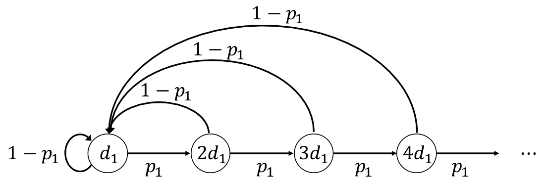
Next, we calculate Δ¯1\bar{\Delta}_{1}. Note that π1\pi_{1} results in an Markov chain with a single recurrent class. The state transition diagram is given in Fig. 4.
Refer to caption
Figure 4. State transition diagram under policy π1\pi_{1} that always choose u=1u=1

Let xlx_{l} be the steady state probability of the state a=l​d1a=ld_{1}, l∈ℕ+l\in\mathbb{N}^{+} when policy π1\pi_{1} is used. Based on the state transition diagram, balance equations can be obtained as follows:

(75) p1xl=xl+1,∀l∈{1,2⋯}.\displaystyle p_{1}x_{l}=x_{l+1},\ \ \ \ \forall l\in\{1,2\cdots\}.

Then, xlx_{l} is expressed as

(76) xl=x1p1l−1,∀l∈{1,2⋯}.\displaystyle x_{l}=x_{1}p_{1}^{l-1},\ \ \ \ \forall l\in\{1,2\cdots\}.

Since ∑l=1∞xl=1\sum_{l=1}^{\infty}x_{l}=1, we obtain x1=1−p1x_{1}=1-p_{1}. Then, under policy π1\pi_{1}, the expected age 𝔼π1​[a]\mathbb{E}_{\pi_{1}}[a] is given by

(77) 𝔼π1​[a]=∑l=1∞l​d1​xl=∑i=1∞l​p1l−1​(1−p1)​d1=11−p1​d1.\displaystyle\mathbb{E}_{\pi_{1}}[a]=\sum_{l=1}^{\infty}ld_{1}x_{l}=\sum_{i=1}^{\infty}lp_{1}^{l-1}(1-p_{1})d_{1}=\frac{1}{1-p_{1}}d_{1}.

Under policy π1\pi_{1}, Yi=d1Y_{i}=d_{1} for all ii. Then, Δ¯1\bar{\Delta}_{1} is given by

(78) Δ¯1\displaystyle\bar{\Delta}_{1} =lim supn→∞∑0n−1𝔼π1​[ai​d1+12​d12]∑i=0n−1𝔼π1​[d1]\displaystyle=\limsup_{n\rightarrow\infty}\frac{\sum_{0}^{n-1}\mathbb{E}_{\pi_{1}}[a_{i}d_{1}+\frac{1}{2}d_{1}^{2}]}{\sum_{i=0}^{n-1}\mathbb{E}_{\pi_{1}}[d_{1}]}
(79) =𝔼π1​[ai]+12​d1\displaystyle=\mathbb{E}_{\pi_{1}}[a_{i}]+\frac{1}{2}d_{1}
(80) =(11−p1+12)​d1.\displaystyle=(\frac{1}{1-p_{1}}+\frac{1}{2})d_{1}.

In a similar way, we obtain Δ¯2=(11−p2+12)​d2\bar{\Delta}_{2}=(\frac{1}{1-p_{2}}+\frac{1}{2})d_{2}. Hence, we obtain an upper bound βmax\beta_{\text{max}} of β\beta, which is given by

βmax=min{Δ¯1,Δ¯2}=min{11−p1+12)d1,(11−p1+12)d2}.\beta_{\text{max}}=\min\{\bar{\Delta}_{1},\bar{\Delta}_{2}\}=\min\Big\{\frac{1}{1-p_{1}}+\frac{1}{2})d_{1},(\frac{1}{1-p_{1}}+\frac{1}{2})d_{2}\Big\}.

Appendix G Proof of Theorem 4.6

(i) We first obtain expression of average cost in (31) with aid of state transition diagram. The state transition diagram under the policy in (14) is given in Fig. 5.

Figure 5. State transition diagram under policy in (14)

Define the state steady probabilities xlx_{l}, xl′x^{\prime}_{l}, zlz_{l} and zl′z^{\prime}_{l} under policy in (14) as

(81) xl≜ℙ⁡(a=d2+l​d2),\displaystyle x_{l}\triangleq\mathbb{P}(a=d_{2}+ld_{2}), 0≤l≤m1+k1,\displaystyle 0\leq l\leq m_{1}+k_{1},
(82) xl′≜ℙ⁡(a=d2+(m1+k1)​d2+l​d1),\displaystyle x^{\prime}_{l}\triangleq\mathbb{P}(a=d_{2}+(m_{1}+k_{1})d_{2}+ld_{1}), l≥0,\displaystyle l\geq 0,
(83) zl≜ℙ⁡(a=d1+l​d2),\displaystyle z_{l}\triangleq\mathbb{P}(a=d_{1}+ld_{2}), 0≤l≤m1,\displaystyle 0\leq l\leq m_{1},
(84) zl′≜ℙ⁡(a=d1+m1​d2+l​d1),\displaystyle z^{\prime}_{l}\triangleq\mathbb{P}(a=d_{1}+m_{1}d_{2}+ld_{1}), l≥0.\displaystyle l\geq 0.

Based on the state transition diagram, balance equations can be obtained as follows:

(85) x0=(1−p2)​(∑l=0m1−1zl+∑l=0m1+k1−1xl),\displaystyle x_{0}=(1-p_{2})\left(\sum_{l=0}^{m_{1}-1}z_{l}+\sum_{l=0}^{m_{1}+k_{1}-1}x_{l}\right),
(86) p2xl=xl+1,l∈{0,1⋯m1+k1−1},\displaystyle p_{2}x_{l}=x_{l+1},\ \ \ \ l\in\{0,1\cdots m_{1}+k_{1}-1\},
(87) p2zl=zl+1,l∈{0,1⋯m1−1},\displaystyle p_{2}z_{l}=z_{l+1},\ \ \ \ l\in\{0,1\cdots m_{1}-1\},
(88) p1xl′=xl+1′,l∈{0,1⋯},\displaystyle p_{1}x^{\prime}_{l}=x^{\prime}_{l+1},\ \ \ \ l\in\{0,1\cdots\},
(89) p1zl=zl+1′,l∈{0,1⋯}.\displaystyle p_{1}z_{l}=z^{\prime}_{l+1},\ \ \ \ l\in\{0,1\cdots\}.

Solving the equations (85)-(89), we obtain the expressions of xlx_{l}, xl′x^{\prime}_{l}, zlz_{l} and zl′z^{\prime}_{l} in terms of x0x_{0} as follows:

(90) xl=p2lx0,l∈{0,1⋯m1+k1},\displaystyle x_{l}=p_{2}^{l}x_{0},\ \ \ \ l\in\{0,1\cdots m_{1}+k_{1}\},
(91) zl=p2m1+k1​p2l1−p2m1x0,l∈{0,1⋯m1},\displaystyle z_{l}=\frac{p_{2}^{m_{1}+k_{1}}p_{2}^{l}}{1-p_{2}^{m_{1}}}x_{0},\ \ \ \ l\in\{0,1\cdots m_{1}\},
(92) xl′=p2m1+k1p1lx0,l∈{0,1⋯},\displaystyle x^{\prime}_{l}=p_{2}^{m_{1}+k_{1}}p_{1}^{l}x_{0},\ \ \ \ l\in\{0,1\cdots\},
(93) zl′=p22​m1+k1​p1l1−p2m1x0,l∈{0,1⋯}.,\displaystyle z^{\prime}_{l}=\frac{p_{2}^{2m_{1}+k_{1}}p_{1}^{l}}{1-p_{2}^{m_{1}}}x_{0},\ \ \ \ l\in\{0,1\cdots\}.,

Substituting (90)-(93) into ∑l=0m1+k1xl+∑l=0m1zl+∑l=1∞xl′+∑l=1∞zl′=1\sum_{l=0}^{m_{1}+k_{1}}x_{l}+\sum_{l=0}^{m_{1}}z_{l}+\sum_{l=1}^{\infty}x^{\prime}_{l}+\sum_{l=1}^{\infty}z^{\prime}_{l}=1, we obtain x0x_{0} as

(94) x0=(1−p1)​(1−p2)​(1−p2m1)1−p1+p2m1​(p1−1)+p2m1+k1​(1−p2).\displaystyle x_{0}=\frac{(1-p_{1})(1-p_{2})(1-p_{2}^{m_{1}})}{1-p_{1}+p_{2}^{m_{1}}(p_{1}-1)+p_{2}^{m_{1}+k_{1}}(1-p_{2})}.

The average cost J1​(m1,k1,β)J_{1}(m_{1},k_{1},\beta) is expressed as

J1​(m1,k1,β)=\displaystyle J_{1}(m_{1},k_{1},\beta)= ∑l=0m1+k1−1C⁡(d2+l​d2,d2)​xl+∑l=0m1−1C⁡(d1+l​d2,d2)​zl\displaystyle\sum_{l=0}^{m_{1}+k_{1}-1}C(d_{2}+ld_{2},d_{2})x_{l}+\sum_{l=0}^{m_{1}-1}C(d_{1}+ld_{2},d_{2})z_{l}
+∑l=0∞C(d2+(m1+k1)d2+ld1,d1)xl′\displaystyle+\sum_{l=0}^{\infty}C(d_{2}+(m_{1}+k_{1})d_{2}+ld_{1},d_{1})x^{\prime}_{l}
(95) +∑l=0∞C(d1+m1d2+ld1,d1)zl′.\displaystyle+\sum_{l=0}^{\infty}C(d_{1}+m_{1}d_{2}+ld_{1},d_{1})z^{\prime}_{l}.

where C⁡(⋅,⋅)C(\cdot,\cdot) is the cost function defined in (11). Substitute (90)-(94) into (95). After some algebraic manipulation and change of variable (p2m1p_{2}^{m_{1}} is replaced by yy), we obtain (31).

Next, we show that J1J_{1} is quasi-convex. By definition of quasi-convex, it suffices to show that its first derivative ∂J1​(y,k1,β)∂y\frac{\partial J_{1}(y,k_{1},\beta)}{\partial y} with respect to yy satisfies at least one of the following conditions [19]:

  • •

    ∂J1​(y,k1,β)∂y≥0\frac{\partial J_{1}(y,k_{1},\beta)}{\partial y}\geq 0

  • •

    ∂J1​(y,k1,β)∂y≤0\frac{\partial J_{1}(y,k_{1},\beta)}{\partial y}\leq 0

  • •

    there exists a point y0∈(0,1]y_{0}\in(0,1] such that for 0<y≤y00<y\leq y_{0}, ∂J1​(y,k1,β)∂y≤0\frac{\partial J_{1}(y;k_{1},\beta)}{\partial y}\leq 0, and for 1≥y≥y01\geq y\geq y_{0}, ∂J1​(y,k1,β)∂y≥0\frac{\partial J_{1}(y;k_{1},\beta)}{\partial y}\geq 0

After some algebraic manipulation, ∂J1​(y,k1,β)∂y\frac{\partial J_{1}(y;k_{1},\beta)}{\partial y} is expressed as

(96) ∂J1​(y,k1,β)∂y=h⁡(y,k1,β)(1−p1+r​y)2\displaystyle\frac{\partial J_{1}(y;k_{1},\beta)}{\partial y}=\frac{h(y;k_{1},\beta)}{(1-p_{1}+ry)^{2}}

where r=−1+p1+p2k1​(1−p2)r=-1+p_{1}+p_{2}^{k_{1}}(1-p_{2}) and h⁡(y,k1,β)h(y;k_{1},\beta) is given by

h⁡(y,k1,β)\displaystyle h(y;k_{1},\beta)\! ≜(A1​y2+D2​yln⁡p2−C1)​r\displaystyle\triangleq\!\Big(A_{1}y^{2}\!+\!\frac{D_{2}y}{\ln p_{2}}\!-\!C_{1}\Big)r\!
(97) +(B1+2​A1​y+D1​(+ln⁡y)ln⁡p2)​(−p2)\displaystyle+\!\Big(B_{1}\!+\!2A_{1}y\!+\frac{D_{1}(1\!+\!\ln y)}{\ln p_{2}}\Big)(1\!-\!p_{2})

Note that the denominator of the (96) is positive. Thus, to show that at least one of the conditions above holds, it suffices to show that h⁡(y,k1,β)h(y;k_{1},\beta) satisfies at least one of the following conditions:

  • •

    B1: h⁡(y,k1,β)≥0h(y;k_{1},\beta)\geq 0;

  • •

    B2: h⁡(y,k1,β)≤0h(y;k_{1},\beta)\leq 0;

  • •

    B3: ∃y0∈(0,1]\exists y_{0}\in(0,1] such that for 0<y≤y00<y\leq y_{0}, h⁡(y,k1,β)≤0h(y;k_{1},\beta)\leq 0, and for 1≥y≥y01\geq y\geq y_{0}, h⁡(y,k1,β)≥0h(y;k_{1},\beta)\geq 0.

In fact, the first derivative of h⁡(y,k1,β)h(y;k_{1},\beta) with respect to yy is

∂h⁡(y,k1,β)∂y\displaystyle\frac{\partial h(y;k_{1},\beta)}{\partial y}
(98) =\displaystyle= (2​(d2​(k1+1)−d1)​y−d2ln⁡p2)⏟G⁡(y)​(r​y+−p1)⏟H⁡(y)​p2k1​Wy\displaystyle\underbrace{\left(2(d_{2}(k_{1}+1)\!-\!d_{1})y-\frac{d_{2}}{\ln p_{2}}\right)}_{G(y)}\underbrace{\left(ry+1\!-p_{1}\right)}_{H(y)}\frac{p_{2}^{k_{1}}W}{y}

where W=d2​(1−p1)−d1​(1−p2)W=d_{2}(1-p_{1})-d_{1}(1-p_{2}). By condition d2​(1−p1)>d1​(1−p2)d_{2}(1-p_{1})>d_{1}(1-p_{2}), W>0W>0. Note that since 0<p1<p2<10<p_{1}<p_{2}<1, r≤−1+p1+(1−p2)=p1−p2<0r\leq-1+p_{1}+(1-p_{2})=p_{1}-p_{2}<0. Thus, H⁡(y)≥r+1−p1=p2k1​(1−p2)>0H(y)\geq r+1-p_{1}=p_{2}^{k_{1}}(1-p_{2})>0, for 0<y≤10<y\leq 1. Hence, ∂h⁡(y,k1,β)∂y\frac{\partial h(y;k_{1},\beta)}{\partial y} is positive (negative) if and only if G⁡(y)G(y) is positive (negative). Next, we will show our finial result by analyzing two different cases.

Case 1: If d2​(k1+1)−d1≥0d_{2}(k_{1}+1)-d_{1}\geq 0, then G⁡(y)≥−d2ln⁡p2>0G(y)\geq-\frac{d_{2}}{\ln p_{2}}>0, for 0<y≤10<y\leq 1. In this case, ∂h⁡(y,k1,β)∂y>0\frac{\partial h(y;k_{1},\beta)}{\partial y}>0, for 0<y≤10<y\leq 1. Thus, h⁡(y,k1,β)h(y;k_{1},\beta) is increasing in yy, for 0<y≤10<y\leq 1. Note that since D1<0D_{1}<0 (by condition d2​(1−p1)>d1​(1−p2)d_{2}(1-p_{1})>d_{1}(1-p_{2})) and p2<1p_{2}<1, we have limy→0h⁡(y,k1,β)=−C1​r+(B1+D1ln⁡p2+limy→0D1​ln⁡yln⁡p2)​(−p2)<0\lim_{y\rightarrow 0}h(y;k_{1},\beta)=-\!C_{1}r+\!\Big(B_{1}\!+\frac{D_{1}}{\ln p_{2}}+\lim_{y\rightarrow 0}\frac{D_{1}\!\ln y}{\ln p_{2}}\Big)(1\!-\!p_{2})<0. Thus, if h⁡(1,k1,β)≤0h(1;k_{1},\beta)\leq 0, then B2 holds; otherwise, B3 holds.

Case 2: If d2​(k1+1)−d1<0d_{2}(k_{1}+1)-d_{1}<0, then G⁡(y)G(y) is decreasing in yy and y1=d22​(d2​(k1+1)−d1)​ln⁡p2>0y_{1}=\frac{d_{2}}{2(d_{2}(k_{1}+1)-d_{1})\ln p_{2}}>0 is a turning point such that G⁡(y)>0G(y)>0 when y<y1y<y_{1} and G⁡(y)<0G(y)<0 when y>y1y>y_{1}.

If y1≥1y_{1}\geq 1, then G⁡(y)≥0G(y)\geq 0 for 0<y≤10<y\leq 1. Thus, ∂h⁡(y,k1,β)∂y≥0\frac{\partial h(y;k_{1},\beta)}{\partial y}\geq 0, which implies that h⁡(y,k1,β)h(y;k_{1},\beta) is increasing in yy for 0<y≤10<y\leq 1. Hence, B2 or B3 holds as explained in case 1.

If y1<1y_{1}<1, then G⁡(y)>0G(y)>0 when y<y1y<y_{1} and G⁡(y)<0G(y)<0 when 1>y>y11>y>y_{1}, which implies h⁡(y,k1,β)h(y;k_{1},\beta) first increases and then decreases for 0<y≤10<y\leq 1. We claim that if y1<1y_{1}<1, then h⁡(1,k1,β)≥0h(1;k_{1},\beta)\geq 0 for β∈[βmin,βmax]\beta\in[\beta_{\text{min}},\beta_{\text{max}}] and k1∈𝒦1k_{1}\in\mathcal{K}_{1}. Recall that limy→0h⁡(y,k1,β)<0\lim_{y\rightarrow 0}h(y;k_{1},\beta)<0. With this, the claim implies that h⁡(y,k1,β)h(y;k_{1},\beta) starts with some negative value and increases to zero at some point y′y^{\prime} and after h⁡(y,k1,β)h(y;k_{1},\beta) becomes positive, it will keep positive for y′<y≤1y^{\prime}<y\leq 1 (B3 holds). It remains to show that our claim holds.

Since y1=d22​(d2​(k1+1)−d1)​ln⁡p2<1y_{1}=\frac{d_{2}}{2(d_{2}(k_{1}+1)-d_{1})\ln p_{2}}<1, we have

(99) d1d2>k1+1−12​ln⁡p2\displaystyle\frac{d_{1}}{d_{2}}>k_{1}+1-\frac{1}{2\ln p_{2}}

After some algebraic manipulation and simplification, h⁡(1,k1,β)h(1;k_{1},\beta) is expressed as

h⁡(1,k1,β)\displaystyle h(1;k_{1},\beta)
=\displaystyle= p22​k1​W​(d2​(k1+1)−d1−d2ln⁡p2)​(1−p2)\displaystyle p_{2}^{2k_{1}}W\left(d_{2}(k_{1}+1)-d_{1}-\frac{d_{2}}{\ln p_{2}}\right)(1-p_{2})
+p2k1​(1−p2)​(1−p1)​((11−p1+0.5)​d12−(11−p2+0.5)​d22)\displaystyle+p_{2}^{k_{1}}(1-p_{2})(1-p_{1})\left((\frac{1}{1-p_{1}}+0.5)d_{1}^{2}-(\frac{1}{1-p_{2}}+0.5)d_{2}^{2}\right)
(100) +p2k1​(d2−d1)​(1−p1)​(1−p2)​β\displaystyle+p_{2}^{k_{1}}(d_{2}-d_{1})(1-p_{1})(1-p_{2})\beta

Since p2k1​(d2−d1)​(1−p1)​(1−p2)<0p_{2}^{k_{1}}(d_{2}-d_{1})(1-p_{1})(1-p_{2})<0, h⁡(1,k1,β)h(1;k_{1},\beta) is decreasing in β\beta and thus h⁡(1,k1,β)≥h⁡(1,k1,βmax)≥h⁡(1,k1,(11−p1+0.5)​d1)h(1;k_{1},\beta)\geq h(1;k_{1},\beta_{\text{max}})\geq h(1;k_{1},(\frac{1}{1-p_{1}}+0.5)d_{1}). It remains to show that h⁡(1,k1,(11−p1+0.5)​d1)≥0h(1;k_{1},(\frac{1}{1-p_{1}}+0.5)d_{1})\geq 0. It is equivalent to show that h⁡(1,k1,(11−p1+0.5)​d1)d22≥0\frac{h(1;k_{1},(\frac{1}{1-p_{1}}+0.5)d_{1})}{d_{2}^{2}}\geq 0 since d22≥0d_{2}^{2}\geq 0. Let z=d1d2z=\frac{d_{1}}{d_{2}}, substitute this into h⁡(1,k1,(11−p1+0.5)​d1)d22\frac{h(1;k_{1},(\frac{1}{1-p_{1}}+0.5)d_{1})}{d_{2}^{2}} and obtain a function of zz denoted by w⁡(z)w(z). By (99), the first derivative of w⁡(z)w(z) satisfies

w′​(z)=\displaystyle w^{\prime}(z)= 2​p22​k1​(1−p2)2​z+p2k1​(1−p2)​(11−p1+0.5)​(1−p1)\displaystyle 2p_{2}^{2k_{1}}(1-p_{2})^{2}z+p_{2}^{k_{1}}(1-p_{2})(\frac{1}{1-p_{1}}+0.5)(1-p_{1})
(101) +\displaystyle+ p22​k1​(1−p2)​(1−p2ln⁡p2−(1−p2)​(k1+1)−(1−p1))\displaystyle p_{2}^{2k_{1}}(1-p_{2})\left(\frac{1-p_{2}}{\ln p_{2}}-(1-p_{2})(k_{1}+1)-(1-p_{1})\right)
(102) ≥\displaystyle\geq w′​(k1+1−12​ln⁡p2)\displaystyle w^{\prime}(k_{1}+1-\frac{1}{2\ln p_{2}})
=\displaystyle= OPENp2k1​(1−p2)​(p2k1​(1−p2)​(k1+1)+1−p12))\displaystyle p_{2}^{k_{1}}(1-p_{2})\left(p_{2}^{k_{1}}(1-p_{2})(k_{1}+1)+\frac{1-p_{1}}{2})\right)
(103) +\displaystyle+ p2k1​(1−p2)​(1−p2k1​(1−p1))\displaystyle p_{2}^{k_{1}}(1-p_{2})\left(1-p_{2}^{k_{1}}(1-p_{1})\right)
(104) >\displaystyle> 0\displaystyle 0

The (104) holds since 0<p1<p2<10<p_{1}<p_{2}<1. Thus, w⁡(z)w(z) is increasing and we have

(105) w⁡(z)≥\displaystyle w(z)\geq w⁡(k1+1−12​ln⁡p2)\displaystyle w(k_{1}+1-\frac{1}{2\ln p_{2}})
=\displaystyle= p2k1​(1−p2)⏟>0​(p2k1​(1−p2)+ln⁡p2)⏟s1​(p2)​(k12​ln⁡p2−14​(ln⁡p2)2)⏟<0\displaystyle\underbrace{p_{2}^{k_{1}}(1-p_{2})}_{>0}\underbrace{\left(p_{2}^{k_{1}}(1-p_{2})+\ln p_{2}\right)}_{s_{1}(p_{2})}\underbrace{\left(\frac{k_{1}}{2\ln p_{2}}-\frac{1}{4(\ln p_{2})^{2}}\right)}_{<0}
(106) +\displaystyle+ p2k12​ln⁡p2​δ​(p1,p2,k1)\displaystyle\frac{p_{2}^{k_{1}}}{2\ln p_{2}}\delta(p_{1},p_{2},k_{1})

where

δ⁡(p1,p2,k1)=\displaystyle\delta(p_{1},p_{2},k_{1})= (p1−p2)​(1−p2)​p2k1+2​(p1−p2)​ln⁡p2\displaystyle(p_{1}-p_{2})(1-p_{2})p_{2}^{k_{1}}+2(p_{1}-p_{2})\ln p_{2}
+2​k1​(1−0.5​p2)​(1−p2)​ln⁡p2+(1−p2)​(0.5​p1−1)\displaystyle+2k_{1}(1-0.5p_{2})(1-p_{2})\ln p_{2}+(1-p_{2})(0.5p_{1}-1)

Note that s1​(p2)≤1−p2+ln⁡p2<0s_{1}(p_{2})\leq 1-p_{2}+\ln p_{2}<0. Thus, to show that w⁡(z)≥0w(z)\geq 0 holds, we only need to show that δ⁡(p1,p2,k1)≤0\delta(p_{1},p_{2},k_{1})\leq 0 holds. Actually,

∂δ⁡(p1,p2,k1)∂p2\displaystyle\frac{\partial\delta(p_{1},p_{2},k_{1})}{\partial p_{2}}
=(p1−p2)​(1−p2)​p2k1​ln⁡p2+k1​(2−p1)​(1p2−1−ln⁡p2)⏟>0​ by ​0<p1<p2<1\displaystyle=\underbrace{(p_{1}-p_{2})(1-p_{2})p_{2}^{k_{1}}\ln p_{2}+k_{1}(2-p_{1})(\frac{1}{p_{2}}-1-\ln p_{2})}_{>0\text{ by }0<p_{1}<p_{2}<1}
(107) +p2k1​(2​p2−1−p1)+2​p1p2−1−p12−2​ln⁡p2⏟θ⁡(p1,p2,k1)\displaystyle+\underbrace{p_{2}^{k_{1}}(2p_{2}-1-p_{1})+\frac{2p_{1}}{p_{2}}-1-\frac{p_{1}}{2}-2\ln p_{2}}_{\theta(p_{1},p_{2},k_{1})}
(108) ≥0\displaystyle\geq 0

where the (108) holds since θ⁡(p1,p2,k1)\theta(p_{1},\!p_{2},\!k_{1}) decreases with p2p_{2} and θ⁡(p1,1,k1)=0.5​p1>0\theta(p_{1},\!1,\!k_{1})=0.5p_{1}>0. Actually,

(109) ∂θ⁡(p1,p2,k1)∂p2\displaystyle\frac{\partial\theta(p_{1},p_{2},k_{1})}{\partial p_{2}} =(2​p2−1−p1)​p2k1​ln⁡p2+2​p2k1−2​p1p22−2p2\displaystyle=(2p_{2}-1-p_{1})p_{2}^{k_{1}}\ln p_{2}+2p_{2}^{k_{1}}-2\frac{p_{1}}{p_{2}^{2}}-\frac{2}{p_{2}}
(110) <(p2−1)​p2k1​ln⁡p2+2​p2k1−2​p1p22−2p2\displaystyle<(p_{2}-1)p_{2}^{k_{1}}\ln p_{2}+2p_{2}^{k_{1}}-2\frac{p_{1}}{p_{2}^{2}}-\frac{2}{p_{2}}
(111) ≤−(p2−1)​p2k1​12​p2+2​p2k1−2​p1p22−2p2\displaystyle\leq-(p_{2}-1)p_{2}^{k_{1}}\frac{1}{2p_{2}}+2p_{2}^{k_{1}}-2\frac{p_{1}}{p_{2}^{2}}-\frac{2}{p_{2}}
(112) ≤−(p2−1)​12​p2+2−2​p1p22−2p2\displaystyle\leq-(p_{2}-1)\frac{1}{2p_{2}}+2-2\frac{p_{1}}{p_{2}^{2}}-\frac{2}{p_{2}}
(113) <0\displaystyle<0

where (110) holds since p2−p1>0p_{2}-p_{1}>0 and ln⁡p2<0\ln p_{2}<0; (111) holds by s2​(x)≜1x+2​ln⁡x≥0s_{2}(x)\triangleq\frac{1}{x}+2\ln x\geq 0 for 0<x≤10<x\leq 1; (112) holds since p2k1≤1p_{2}^{k_{1}}\leq 1; (112) holds since p2<1p_{2}<1. In particular, the first derivative of s2s_{2} is s2′​(x)=−1x2+2xs_{2}^{\prime}(x)=-\frac{1}{x^{2}}+\frac{2}{x}. Thus, s2s_{2} decreases when x≤0.5x\leq 0.5 (since s2′​(x)≤0s_{2}^{\prime}(x)\leq 0 when x≤0.5x\leq 0.5) and then increases when x≥0.5x\geq 0.5 (since s2′​(x)≥0s_{2}^{\prime}(x)\geq 0 when x≥0.5x\geq 0.5) . Thus, s2​(x)≥s2​(0.5)=0.2213>0s_{2}(x)\geq s_{2}(0.5)=0.2213>0. By (108), δ\delta increases with p2p_{2} and δ⁡(p1,p2,k1)≤δ⁡(p1,1,k1)=0\delta(p_{1},p_{2},k_{1})\leq\delta(p_{1},1,k_{1})=0. This completes the proof of part (i).

(ii) If d1​(1−p2)≥d2​(1−p1)d_{1}(1-p_{2})\geq d_{2}(1-p_{1}), the optimal policy is of threshold-type in (15). Similar to part (i), with aid of state transition diagram, we obtain the expression of average cost J2J_{2} under policy (15) as

(114) J2​(m2,k2,β)=A2​p12​m2+B2​p1m2+C2+D2​m2​p1m21−p2+(1−p1−p1k2​(1−p2))​p1m2.J_{2}(m_{2},k_{2},\beta)=\frac{A_{2}p_{1}^{2m_{2}}+B_{2}p_{1}^{m_{2}}+C_{2}+D_{2}m_{2}p_{1}^{m_{2}}}{1-p_{2}+(1-p_{1}-p_{1}^{k_{2}}(1-p_{2}))p_{1}^{m_{2}}}.

In particular, the state transition diagram under policy in (15) is given in Fig. 6.

Figure 6. State transition diagram under policy in (15)

Define the steady state probabilities xlx_{l}, xl′x^{\prime}_{l}, yly_{l} and yl′y^{\prime}_{l} under policy in (15) as

(115) xl≜ℙ⁡(a=d1+l​d1),\displaystyle x_{l}\triangleq\mathbb{P}(a=d_{1}+ld_{1}), 0≤l≤m2,\displaystyle 0\leq l\leq m_{2},
(116) xl′≜ℙ⁡(a=d1+m2​d1+l​d2),\displaystyle x^{\prime}_{l}\triangleq\mathbb{P}(a=d_{1}+m_{2}d_{1}+ld_{2}), l≥0,\displaystyle l\geq 0,
(117) zl≜ℙ⁡(a=d2+l​d1),\displaystyle z_{l}\triangleq\mathbb{P}(a=d_{2}+ld_{1}), 0≤l≤m2+k2,\displaystyle 0\leq l\leq m_{2}+k_{2},
(118) zl′≜ℙ⁡(a=d2+(m2+k2)​d1+l​d2),\displaystyle z^{\prime}_{l}\triangleq\mathbb{P}(a=d_{2}+(m_{2}+k_{2})d_{1}+ld_{2}), l≥0.\displaystyle l\geq 0.

Based on the state transition diagram, balance equations can be obtained as follows:

(119) x0=(1−p1)​(∑l=0m2−1xl+∑l=0m2+k2−1zl),\displaystyle x_{0}=(1-p_{1})\left(\sum_{l=0}^{m_{2}-1}x_{l}+\sum_{l=0}^{m_{2}+k_{2}-1}z_{l}\right),
(120) p1xl=xl+1,l∈{0,1⋯m2−1},\displaystyle p_{1}x_{l}=x_{l+1},\ \ \ \ l\in\{0,1\cdots m_{2}-1\},
(121) p1zl=zl+1,l∈{0,1⋯m2+k2−1},\displaystyle p_{1}z_{l}=z_{l+1},\ \ \ \ l\in\{0,1\cdots m_{2}+k_{2}-1\},
(122) p2xl′=xl+1′,l∈{0,1⋯},\displaystyle p_{2}x^{\prime}_{l}=x^{\prime}_{l+1},\ \ \ \ l\in\{0,1\cdots\},
(123) p2zl′=zl+1′,l∈{0,1⋯}.\displaystyle p_{2}z^{\prime}_{l}=z^{\prime}_{l+1},\ \ \ \ l\in\{0,1\cdots\}.

Solving the equations (119)-(123), we obtain the expressions of xlx_{l}, xl′x^{\prime}_{l}, zlz_{l} and zl′z^{\prime}_{l} in terms of x0x_{0} as follows:

(124) xl=p1lx0,l∈{0,1⋯m2},\displaystyle x_{l}=p_{1}^{l}x_{0},\ \ \ \ l\in\{0,1\cdots m_{2}\},
(125) zl=p1m2​p1l1−p1m2+k2x0,l∈{0,1⋯m2+k2},\displaystyle z_{l}=\frac{p_{1}^{m_{2}}p_{1}^{l}}{1-p_{1}^{m_{2}+k_{2}}}x_{0},\ \ \ \ l\in\{0,1\cdots m_{2}+k_{2}\},
(126) xl′=p1m2p2lx0,l∈{0,1⋯},\displaystyle x^{\prime}_{l}=p_{1}^{m_{2}}p_{2}^{l}x_{0},\ \ \ \ l\in\{0,1\cdots\},
(127) zl′=p12​m2+k2​p2l1−p1m2+k2x0,l∈{0,1⋯}.,\displaystyle z^{\prime}_{l}=\frac{p_{1}^{2m_{2}+k_{2}}p_{2}^{l}}{1-p_{1}^{m_{2}+k_{2}}}x_{0},\ \ \ \ l\in\{0,1\cdots\}.,

Substituting (124)-(127) into ∑l=0m2−1xl+∑l=0m2+k2−1zl+∑l=0∞xl′+∑l=0∞zl′=1\sum_{l=0}^{m_{2}-1}x_{l}+\sum_{l=0}^{m_{2}+k_{2}-1}z_{l}+\sum_{l=0}^{\infty}x^{\prime}_{l}+\sum_{l=0}^{\infty}z^{\prime}_{l}=1, we obtain x0x_{0} as

(128) x0=(1−p1)​(1−p2)​(1−p1m2+k2)1−p2+p1m2+k2​(p2−1)+p1m2​(1−p1).\displaystyle x_{0}=\frac{(1-p_{1})(1-p_{2})(1-p_{1}^{m_{2}+k_{2}})}{1-p_{2}+p_{1}^{m_{2}+k_{2}}(p_{2}-1)+p_{1}^{m_{2}}(1-p_{1})}.

The average cost J2​(m2,k2,β)J_{2}(m_{2},k_{2},\beta) is expressed as

J2​(m2,k2,β)=\displaystyle J_{2}(m_{2},k_{2},\beta)= ∑l=0m2−1C⁡(d1+l​d1,d1)​xl+∑l=0m2+k2−1C⁡(d2+l​d1,d1)​zl\displaystyle\sum_{l=0}^{m_{2}-1}C(d_{1}+ld_{1},d_{1})x_{l}+\sum_{l=0}^{m_{2}+k_{2}-1}C(d_{2}+ld_{1},d_{1})z_{l}
+∑l=0∞C(d1+m2d1+ld2,d2)xl′\displaystyle+\sum_{l=0}^{\infty}C(d_{1}+m_{2}d_{1}+ld_{2},d_{2})x^{\prime}_{l}
(129) +∑l=0∞C(d2+(m2+k2)d1+ld2,d2)zl′.\displaystyle+\sum_{l=0}^{\infty}C(d_{2}+(m_{2}+k_{2})d_{1}+ld_{2},d_{2})z^{\prime}_{l}.

Substitute (124)-(128) into (129). After some algebraic manipulation and simplification, we obtain (114).

Next, we show that the optimal policy that solves (30) chooses u=2u=2 at each transmission opportunity, which is equivalent to show that m2=0m_{2}=0 and n2=0n_{2}=0. In particular, (1) we show that for any m2m_{2}, J2​(m2,k2,β)J_{2}(m_{2},k_{2},\beta) is non-decreasing in k2k_{2}, which implies that optimal k2k_{2} equals zero; (2) we show that J2​(m2,0,β)J_{2}(m_{2},0,\beta) is non-decreasing in m2m_{2}. This implies that optimal m2m_{2} equals zero. Since n2=m2+k2n_{2}=m_{2}+k_{2}, then optimal n2n_{2} equals to zero and thus the optimal average cost is J2​(0,0,β)J_{2}(0,0,\beta), which will complete the proof of part (ii). The proof is specified as follows:

(1) We show that any m2m_{2}, J2​(m2,k2,β)J_{2}(m_{2},k_{2},\beta) is non-decreasing in k2k_{2}. Since k2∈𝒦2={0,1}k_{2}\in\mathcal{K}_{2}=\{0,1\}, it suffices to show that J2​(m2,1,β)−J2​(m2,0,β)≥0J_{2}(m_{2},1,\beta)-J_{2}(m_{2},0,\beta)\geq 0. Using the expression of J2J_{2} in (114), after some algebraic manipulation, we get

(130) J2​(m2,1,β)−J2​(m2,0,β)=p12​m2​g1​(m2,β)F1​(m2)\displaystyle J_{2}(m_{2},1,\beta)-J_{2}(m_{2},0,\beta)=\frac{p_{1}^{2m_{2}}g_{1}(m_{2},\beta)}{F_{1}(m_{2})}

where

g1​(m2,β)\displaystyle g_{1}(m_{2},\beta)
=\displaystyle= p1m2​((−p1)2​d2−d1​(1−p1)+p1​d1​(−p2))​E\displaystyle p_{1}^{m_{2}}\Big(\left(1\!-\!p_{1}\right)^{2}d_{2}-d_{1}(1-p_{1})+p_{1}d_{1}(1\!-\!p_{2})\Big)E
+m2​d1​(1−p1)​(1−p2)​E\displaystyle+m_{2}d_{1}(1-p_{1})(1-p_{2})E
+(1−p1)2​(1−p2)​((d2−d1)​β+d1​β1−d2​β2)\displaystyle+(1-p_{1})^{2}(1-p_{2})\big((d_{2}-d_{1})\beta+d_{1}\beta_{1}-d_{2}\beta_{2}\big)
(131) +((−p1)​d2−d1)​(1−p2)​E+(d1−d2)​(1−p1)​(1−p2)​E\displaystyle+\big(\left(1\!-\!p_{1}\right)d_{2}-d_{1}\big)(1-p_{2})E+(d_{1}-d_{2})(1-p_{1})(1-p_{2})E

where β1=11−p1​d1+0.5​d1\beta_{1}=\frac{1}{1-p_{1}}d_{1}+0.5d_{1}, β2=11−p2​d2+0.5​d2\beta_{2}=\frac{1}{1-p_{2}}d_{2}+0.5d_{2}, and E=d1​(1−p2)−d2​(1−p1)E=d_{1}(1-p_{2})-d_{2}(1-p_{1}); and F1​(m2)F_{1}(m_{2}) is given by

(132) F1​(m2)=(−p2+p1m2​(−2​p1+p1​p2))​(−p2+p1m2​(p2−p1))\displaystyle F_{1}(m_{2})=\big(1\!-\!p_{2}\!+\!p_{1}^{m_{2}}(1\!-\!2p_{1}+p_{1}p_{2})\big)\big(1\!-\!p_{2}+p_{1}^{m_{2}}(p_{2}\!-\!p_{1})\big)

Since p1<p2<1p_{1}<p_{2}<1, we have that 1−2​p1+p1​p2=1−p1−p1​(1−p2)≥1−p1−(1−p2)≥01-2p_{1}+p_{1}p_{2}=1-p_{1}-p_{1}(1-p_{2})\geq 1-p_{1}-(1-p_{2})\geq 0. It means that F1F_{1} is a product of two non-negative expressions and thus we have F1​(m2)≥0F_{1}(m_{2})\geq 0, for all m2m_{2}. Hence, to show the result, we only need to show that g1​(m2,β)≥0g_{1}(m_{2},\beta)\geq 0 holds. In particular, we have

(−p1)2​d2−d1​(1−p1)+p1​d1​(−p2)\displaystyle\left(1\!-\!p_{1}\right)^{2}d_{2}-d_{1}(1-p_{1})+p_{1}d_{1}(1\!-\!p_{2})
(133) ≤\displaystyle\leq (−p1)2​d2−d1​(1−p2)+p1​d1​(−p2)\displaystyle\left(1\!-\!p_{1}\right)^{2}d_{2}-d_{1}(1-p_{2})+p_{1}d_{1}(1\!-\!p_{2})
(134) =\displaystyle= (−p1)​(d2​(−p1)−d1​(−p2))\displaystyle\left(1\!-\!p_{1}\right)(d_{2}\left(1\!-\!p_{1}\right)-d_{1}\left(1\!-\!p_{2}\right))
(135) ≤\displaystyle\leq 0\displaystyle 0

where (133) holds since 0<p1<p2<10<p_{1}<p_{2}<1, and (135) holds due to condition d1​(1−p2)≥d2​(1−p1)d_{1}(1-p_{2})\geq d_{2}(1-p_{1}) and p1<1p_{1}<1. In addition, by condition d1​(1−p2)≥d2​(1−p1)d_{1}(1-p_{2})\geq d_{2}(1-p_{1}), we get E≥0E\geq 0. Thus, the first term in (131) satisfies

p1m2​((−p1)2​d2−d1​(1−p1)+p1​d1​(−p2))​E\displaystyle p_{1}^{m_{2}}\Big(\left(1\!-\!p_{1}\right)^{2}d_{2}-d_{1}(1-p_{1})+p_{1}d_{1}(1\!-\!p_{2})\Big)E
(136) ≥\displaystyle\geq ((−p1)2​d2−d1​(1−p1)+p1​d1​(−p2))​E\displaystyle\Big(\left(1\!-\!p_{1}\right)^{2}d_{2}-d_{1}(1-p_{1})+p_{1}d_{1}(1\!-\!p_{2})\Big)E

Moreover, the second term in (131) satisfies

(137) m2​d1​(1−p1)​(1−p2)​E≥0\displaystyle m_{2}d_{1}(1-p_{1})(1-p_{2})E\geq 0

Recall that β1=11−p1​d1+0.5​d1\beta_{1}=\frac{1}{1-p_{1}}d_{1}+0.5d_{1}, β2=11−p2​d2+0.5​d2\beta_{2}=\frac{1}{1-p_{2}}d_{2}+0.5d_{2} and βm​a​x=min⁡{β1,β2}\beta_{max}=\min\{\beta_{1},\beta_{2}\}. Since d1>d2d_{1}>d_{2} and d1​(1−p2)≥d2​(1−p1)d_{1}(1-p_{2})\geq d_{2}(1-p_{1}), we have β1≥β2\beta_{1}\geq\beta_{2}. Hence, β≤βm​a​x=min⁡{β1,β2}=β2\beta\leq\beta_{max}=\min\{\beta_{1},\beta_{2}\}=\beta_{2}. Moreover, since d2<d1d_{2}<d_{1} and 0<p1<p2<10<p_{1}<p_{2}<1, we have (1−p1)2​(1−p2)​(d2−d1)<0(1-p_{1})^{2}(1-p_{2})(d_{2}-d_{1})<0. Hence, the third term in (131) satisfies

(138) (1−p1)2​(1−p2)​(d2−d1)​β≥(1−p1)2​(1−p2)​(d2−d1)​β2\displaystyle(1-p_{1})^{2}(1-p_{2})(d_{2}-d_{1})\beta\geq(1-p_{1})^{2}(1-p_{2})(d_{2}-d_{1})\beta_{2}

Substitute (136), (137) and (138) into (131), after some algebraic manipulation, we get

g1​(m2,β)≥\displaystyle g_{1}(m_{2},\beta)\geq E​d1​(1−p1)​(1−p2)+E​(1−p1)2​d2\displaystyle Ed_{1}(1-p_{1})(1-p_{2})+E(1-p_{1})^{2}d_{2}
(139) +0.5​d1​(1−p1)2​(1−p2)​(d1−d2)\displaystyle+0.5d_{1}(1-p_{1})^{2}(1-p_{2})(d_{1}-d_{2})
(140) ≥\displaystyle\geq 0\displaystyle 0

where (140) holds by E≥0E\geq 0, d1>d2>0d_{1}>d_{2}>0 and 0<p1<p2<10<p_{1}<p_{2}<1.

(2) We show that J2​(m2,0,β)J_{2}(m_{2},0,\beta) is non-decreasing in m2m_{2} by showing J2​(m2+1,0,β)−J2​(m2,0,β)≥0J_{2}(m_{2}+1,0,\beta)-J_{2}(m_{2},0,\beta)\geq 0, for all m2∈ℕm_{2}\in\mathbb{N}. Using the expression of J2J_{2} in (114), after some algebraic manipulation, we get

(141) J2​(m2+1,0,β)−J2​(m2,0,β)=g2​(m2,β)​p1m2F2​(m2)\displaystyle J_{2}(m_{2}+1,0,\beta)-J_{2}(m_{2},0,\beta)=\frac{g_{2}(m_{2},\beta)p_{1}^{m_{2}}}{F_{2}(m_{2})}

where

g2​(m2,β)\displaystyle g_{2}(m_{2},\beta)
=\displaystyle= p12​m2+1​(d2−d1)​(1−p1)​(p2−p1)​E−p1m2+1​d1​(p2−p1)​E\displaystyle p_{1}^{2m_{2}+1}(d_{2}-d_{1})(1-p_{1})(p_{2}-p_{1})E-p_{1}^{m_{2}+1}d_{1}(p_{2}-p_{1})E
+p1m2​(d2−d1)​(1−p12)​(1−p2)​E+m2​d1​(1−p1)​(1−p2)​E\displaystyle+p_{1}^{m_{2}}(d_{2}-d_{1})(1-p_{1}^{2})(1-p_{2})E+m_{2}d_{1}(1-p_{1})(1-p_{2})E
+(1−p1)2​(1−p2)​((d2−d1)​β+d1​β1−d2​β2)\displaystyle+(1-p_{1})^{2}(1-p_{2})\big((d_{2}-d_{1})\beta+d_{1}\beta_{1}-d_{2}\beta_{2}\big)
(142) +(d1−d2)​(1−p1)​(1−p2)​E−d1​p1​(1−p2)​E,\displaystyle+(d_{1}-d_{2})(1-p_{1})(1-p_{2})E-d_{1}p_{1}(1-p_{2})E,

and F2​(m2)F_{2}(m_{2}) is given by

(143) F2​(m2)=(−p2+p1m2+1​(p2−p1))​(−p2+p1m2​(p2−p1)).\displaystyle F_{2}(m_{2})=\big(1\!-\!p_{2}\!+\!p_{1}^{m_{2}+1}(p_{2}-p_{1})\big)\big(1\!-\!p_{2}+p_{1}^{m_{2}}(p_{2}\!-\!p_{1})\big).

Since p1<p2<1p_{1}<p_{2}<1, F2F_{2} is a product of two non-negative terms and thus F2​(m2)≥0F_{2}(m_{2})\geq 0, for all m2m_{2}. Hence, to show the result, we only need to show that g2​(m2,β)≥0g_{2}(m_{2},\beta)\geq 0 holds. In particular, since 0<p1<p2<10<p_{1}<p_{2}<1 and d1>d2d_{1}>d_{2}, the first four terms in (142) satisfy

p12​m2+1​(d2−d1)​(1−p1)​(p2−p1)​E−p1m2+1​d1​(p2−p1)​E\displaystyle p_{1}^{2m_{2}+1}(d_{2}-d_{1})(1-p_{1})(p_{2}-p_{1})E-p_{1}^{m_{2}+1}d_{1}(p_{2}-p_{1})E
+p1m2​(d2−d1)​(1−p12)​(1−p2)​E+m2​d1​(1−p1)​(1−p2)​E\displaystyle+p_{1}^{m_{2}}(d_{2}-d_{1})(1-p_{1}^{2})(1-p_{2})E+m_{2}d_{1}(1-p_{1})(1-p_{2})E
≥\displaystyle\geq p1​(d2−d1)​(1−p1)​(p2−p1)​E−p1​d1​(p2−p1)​E\displaystyle p_{1}(d_{2}-d_{1})(1-p_{1})(p_{2}-p_{1})E-p_{1}d_{1}(p_{2}-p_{1})E
(144) +(d2−d1)​(1−p12)​(1−p2)​E\displaystyle+(d_{2}-d_{1})(1-p_{1}^{2})(1-p_{2})E

Substitute (138) and (144) into (142), after some algebraic manipulation, we get

g2​(m2,β)≥\displaystyle g_{2}(m_{2},\beta)\geq (1−p1)2​(d1​(1−p1)+d2​p1)​E\displaystyle(1-p_{1})^{2}\big(d_{1}(1-p_{1})+d_{2}p_{1}\big)E
(145) +0.5​(1−p1)2​(1−p2)​(d1−d2)​d1\displaystyle+0.5(1-p_{1})^{2}(1-p_{2})(d_{1}-d_{2})d_{1}
(146) ≥\displaystyle\geq 0\displaystyle 0

where (146) holds by E≥0E\geq 0, d1>d2>0d_{1}>d_{2}>0 and 0<p1<p2<10<p_{1}<p_{2}<1.