A tool to predict coercivity in magnetic materials
Abstract
Magnetic coercivity is often viewed to be lower in alloys with negligible (or zero) values of the anisotropy constant. However, this explains little about the dramatic drop in coercivity in FeNi alloys at a non-zero anisotropy value. Here, we develop a theoretical and computational tool to investigate the fundamental interplay between material constants that govern coercivity in bulk magnetic alloys. The two distinguishing features of our coercivity tool are that: (a) we introduce a large localized disturbance, such as a spike-like magnetic domain, that provides a nucleation barrier for magnetization reversal; and (b) we account for magneto-elastic energy—however small—in addition to the anisotropy and magnetostatic energy terms. We apply this coercivity tool to show that the interactions between local instabilities and material constants, such as anisotropy and magnetostriction constants, are key factors that govern magnetic coercivity in bulk alloys. Using our model, we show that coercivity is minimum at the permalloy composition () at which the alloy’s anisotropy constant is not zero. We systematically vary the values of the anisotropy and magnetostriction constants, around the permalloy composition, and identify new combinations of material constants at which coercivity is small. More broadly, our coercivity tool provides a theoretical framework to potentially discover novel magnetic materials with low coercivity.
1 Introduction
In ferromagnetic materials, hysteresis is the lag in reorienting the magnetic moment with the applied field. This reorientation is typically delayed with respect to the applied field, and follows a characteristic curve as shown in Fig. 1. This phenomenon is called hysteresis, and the corresponding curve is called the hysteresis loop. The width of this hysteresis loop determines several applications of magnetic materials. For example, magnetic alloys with narrow hysteresis width, informally called soft magnets, are used in transformer cores and induction motors while magnetic alloys with wide hysteresis width, called hard magnets, are used in permanent magnets and some computer memories [1, 2]. Other features of the hysteresis loop—such as magnetic saturation, coercive field (with magnitude termed coercivity), and remnant magnetization—govern the applications of magnetic alloys.

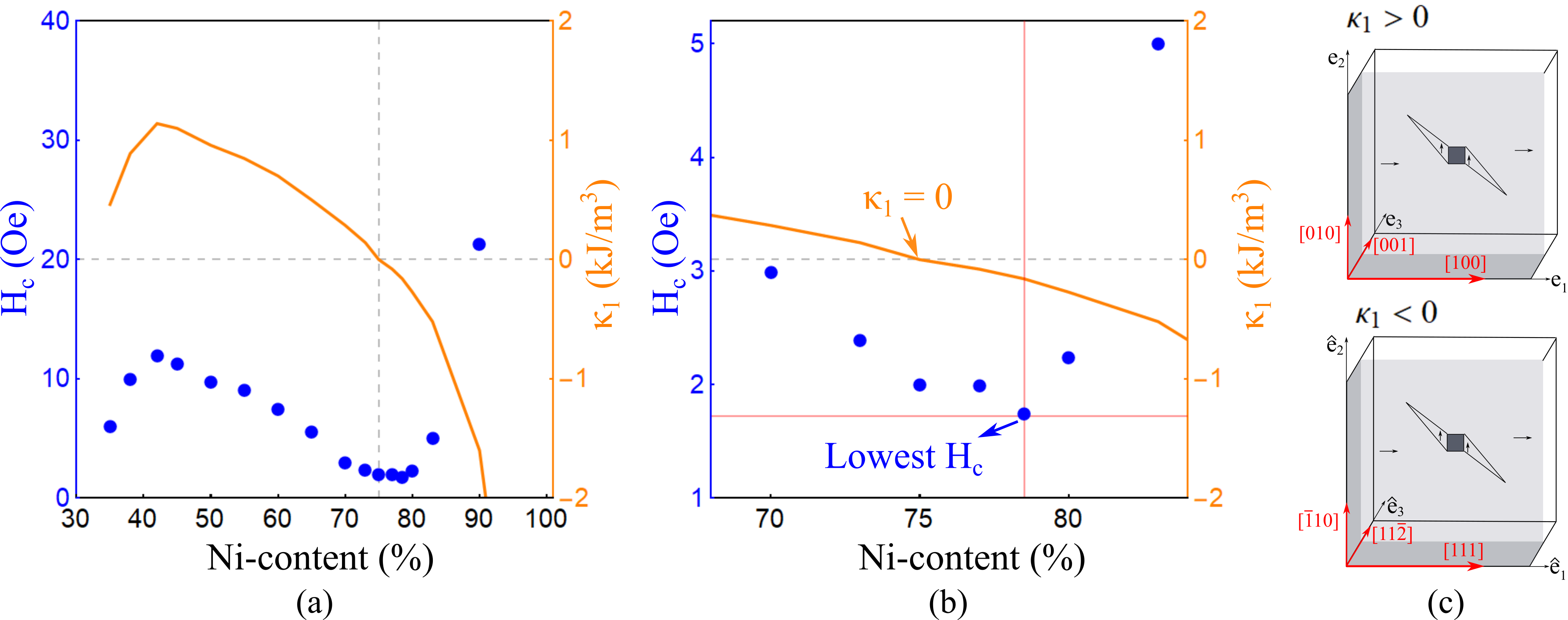
Although hysteresis is a fundamental property that governs the application of magnetic materials, we know little about the fundamental constants that govern hysteresis [3]. For example, a commonly accepted reasoning for low hysteresis in magnetic alloys focuses on a material constant , called the anisotropy constant. This constant penalizes the magnetization rotation away from its preferred crystallographic orientation. At present, theoretical methods suggest that a small (or zero) anisotropy constant lowers magnetic hysteresis [4, 5, 6]. However, this reasoning contradicts experimental observations: Take the well studied FeNi binary alloy system [7]. In this alloy system, magnetic hysteresis is drastically lowered at 78.5 Ni-content. However, the anisotropy constant at this composition is not zero. In fact, the anisotropy constant is zero at 75 Ni-content, at which magnetic hysteresis is not minimum. Also, magnetostriction constants vanish at nearby compositions, but not at 78.5 Ni. These discrepancies in the FeNi system are known as the “Permalloy Problem”[7, 8]. Similar discrepancies are observed in other magnetic systems, such as the Sendust, FeGa and NiMnGa alloys [9, 11, 10, 12]. These examples suggest that we understand little of the role of material constants that govern magnetic hysteresis in bulk alloys. It is, therefore, important to develop a theoretical and computational framework that reliably predicts magnetic coercivity in bulk magnetic alloys. Such a framework would open doors to developing novel magnetic alloys with low hysteresis.
1.1 Mathematical modeling of magnetic hysteresis
A widely used theory to describe magnetization processes is the micromagnetics [20]. This is a continuum theory that describes the energy of a body in terms of its magnetic moment. In this theory, each energy term is directly correlated with a measured material constant, and potentially provides a rigorous framework for exploring the links between material constants and magnetic hysteresis. Attempts to use the micromagnetics to understand hysteresis have a long history: Beginning in the 1950s [14, 15, 16, 17], researchers studied the breakdown of a single domain state under a constant external field. They decreased the magnitude of this external field from a large value. In this method, a typical approach was to consider the second variation of the micromagnetics energy evaluated at a constant magnetization in equilibrium with the constant applied field, i.e., linear stability analysis [20]. This leads to a linear partial differential equation in the form of an eigenvalue problem, with non-trivial solutions associated to breakdown. With the aid of simplifications (ellipsoids), these linear equations could sometimes be solved analytically, and the results were studied sufficiently intensely so that the eigenvectors were given names such as coherent rotation, magnetization curling, and anticurling [15, 16, 17]. (For a modern treatment of these kinds of calculations based on duality, see Section 8 of [31].)
The well-known difficulty with this approach is that, when accepted values for the material constants are substituted into the results, they dramatically over predict the coercivity [20, 13]. A typical evaluation in iron is a coercivity of , where is the first anisotropy constant, is the constant magnetization and is an appropriate demagnetization matrix for the region of interest. For a typical bulk specimen of iron, this gives a coercivity more than three orders of magnitude higher than the measured value. This general disagreement between the results of linear stability analysis and experiment was termed the Coercivity Paradox [20]. On the other hand, it was later recognized that in certain perfect single crystals with atomically smooth boundaries and in similarly perfect nanostructures, coercivities approaching the results of linear stability analysis could be achieved [18].
1.2 Nucleation barriers and localized disturbances
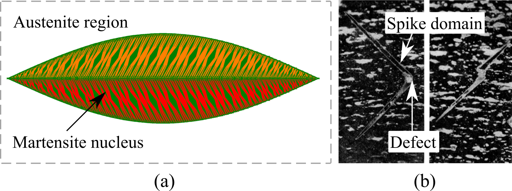
Two recent developments suggest a way forward to predict hysteresis in bulk materials. The first concerns the hysteresis observed in martensitic phase transformations [24]. The goal in that case is to predict the thermal hysteresis on heating and cooling. Like the magnetic case, linear stability analysis fails in the case of martensitic transformations; the linearized operator is typically strongly positive-definite at the point of transformation on cooling, especially in cases of big first order phase transformations. However, if one analyzes a certain nucleus consisting of a twinned platelet (see Fig. 2a for an example), then one finds a realistic energy barrier [38, 23, 24]. More importantly, a simple criterion for lowering this barrier emerges, involving the middle eigenvalue of the transformation stretch matrix [25, 26]. Satisfying this criterion to high accuracy in alloy development programs has led to numerous alloys with near zero thermal hysteresis despite having transformation strains of the order of 10.
The second development suggesting a way forward is an unpublished Ph.D. thesis of N. Pilet [27]. Pilet examines the appearance of the nuclei of reverse domains on the shoulder of the hysteresis loop in various ferromagnetic materials. These nuclei appear precisely at the same location in the material on each magnetization reversal cycle. He finds 1) a strong correlation between the appearance of these nuclei and the ultimate measured coercivity, even though the shoulder occurs at quite a different field than the coercive field, and 2) that the nuclei are large but highly localized disturbances, which in our view would likely not be captured by linear stability analysis.
Theoretically, there are few general methods that treat large localized disturbances. Classical results in the calculus of variations related to “strong relative” minimizers would seem to be relevant, but they are only available in the case of a one-dimensional domain [40]. Recently, a big step forward is the development of a theory of strong local minimizers in the multidimensional case [42, 41]. However, the necessary and sufficient conditions for a strong local minima given by these studies involve the concepts of “quasiconvexity” and “quasiconvexity at the boundary”, which are difficult or impossible to verify with known methods. Another point is that of strong local minimizers are not precisely what is needed in the present case of micromagnetics. That’s because domain wall energy dominates at small scales, so typical large localized disturbances always increase the energy at sufficiently small scales, i.e., they are missed by the usual concept of “strong local minimizer”. It is the barrier that is important, and, in the present case, the dependence of the height of the barrier on material constants. To our knowledge, the only general approach to estimation of the barrier (in the case of phase transformations) is the work of Knüpfer, Kohn and Otto [38, 39].
1.3 Present research
In the present work, we develop a computational tool that predicts coercivity in bulk magnetic alloys. To this end, we use the concept of nucleation barriers to compute magnetic hysteresis. As in the martensitic case, the key is to select a potent defect. In magnetic materials, inclusions in the form of a spike domain are commonly found around defects, and possess a fine needle-like geometry, see Fig. 2(b) [30]. These spike-domains form to minimize the total energy of the system. They were theoretically predicted to form by Néel [28] and have been imaged by Williams [29]. We hypothesize that these spike-domain microstructures serve as a nucleus (or a local disturbance) that grows during magnetization reversal. Unlike in shape memory alloys in which the needle growth is a balance between elastic and interfacial energies, the growth of a spike-domain in alloys with strong ferromagnetism involves an intricate balance between anisotropy, magnetostatic, and magnetostrictive energies. Except for introducing this physically motivated defect, we do not introduce other perturbations, random or deterministic, to seed the magnetization reversal process. In this sense we are formulating a method that specifically tests the potency of spatial defects as a possible cause of hysteresis in the absence of mechanisms involving thermal activation. Although one could choose infinitely many possible defects, our predictions of hysteresis using the spike domain substantiate the intuition of Néel that the spike domain is the potent defect.
The structure of the remainder of this paper is as follows: In Section 2, we give an overview of micromagnetics and equilibrium equations that are implemented in our computational tool. Here, we account for the magnetoelastic energy terms that were typically neglected in prior calculations; and we introduce concepts related to ellipsoid theorem and reciprocal theorem that simplify our calculation for computing magnetic coercivity. A key aspect is to find a computational way to model the important effect of boundaries that are typically far from the defect but play an important role. Next, in Section 3 we demonstrate the advantages of this computational tool across three case studies: (a) We show how the tool can be applied to modeling stress in magnetic alloys, and in doing so uncover that the effect of stress on hysteresis varies as a function of alloy composition. (b) We show how the tool can be applied to engineering different defect geometries, and by doing so we find how the structural features of defects affect hysteresis loops. (c) We show how applying the tool can help solve the Permalloy problem. (d) We reveal an unexpectedly important effect of magnetostriction on hysteresis, contrary to the conventional wisdom that, all else fixed, coercivity is minimized at vanishing magnetostriction constants. Broadly, we find that the delicate balance between material constants, such as the magnetostriction and the anisotropy constant, has an important influence on coercivity.
Overall, we present a computational framework to predict coercivity in bulk magnetic alloys. Our tool can be used to discover possible new soft magnetic materials (low hysteresis). In principle, some aspects of our methods could also be used to discover hard magnetic materials (i.e., candidates for permanent magnets) but this is much more difficult: for soft magnets one has only to make a good choice of potent defect, while hard magnets have to exhibit large hysteresis for all possible defects.
2 Theory
In this section, we describe the theoretical framework of our coercivity tool. First, we introduce the total energy of micromagnetics, including magnetostriction. Then we solve the mechanical and magnetostatic equilibrium equations to compute the strain and demagnetization fields, respectively, in the body. Here, we present a computational trick based on the ellipsoid theorem that simplifies the calculation of demagnetization fields in ellipsoid bodies that are much bigger than the defect, but play a critical role. Finally, we compute the evolution of the magnetization using the Landau-Lifshitz-Gilbert equation. This equation is numerically solved using the Gauss-Siedel projection method [32], and the accompanying equilibrium equations are solved in Fourier space [33].

2.1 Micromagnetics
Micromagnetics is a continuum theory that uses the magnetic moment to describe the free energy of a magnetic body [19, 20, 21]. This theory has been successfully applied to solve various problems, such as finding energy minimizing domain structures and understanding their role in the magnetization process [36, 37, 32, 11, 34]. A key advantage of this theory is that the total energy is expressed in terms of conventional material constants that are measured in specific experiments. This advantage of micromagnetics makes it an ideal framework to investigate the links between material constants, microstructural geometry, and magnetic coercive fields. In our coercivity tool, we use the standard micromagnetic energy including magnetostriction and define the free energy function as:
| (1) |
Here, we describe the micromagnetic energy in a cubic basis , where the magnetization, is normalized by its saturation magnetization such that . Eq. 1 describes the energy landscape of a magnetic body, and its local minima represent metastable magnetization patterns. Fig. 3 schematically illustrates the different energy contributions in Eq. 1. First, the exchange energy, penalizes gradients of the magnetization, see Fig. 3(a). This penalty originates from the quantum mechanical exchange-interaction forces between neighboring magnetization, and is minimized when the neighboring magnetization are parallel. Second, the anisotropy energy penalizes magnetization that are not aligned in the direction of easy crystallographic axes, see Fig. 3(b). Here, we assume a cubic form of the anisotropy energy, and is the anisotropy constant. (More general forms can be included without difficulty.) Third, the elastic energy is related to the magnetostrictive response of the material. For example, take a magnetic rod with randomly oriented domains as shown in Fig. 3(c). Next, apply a magnetic field to the rod to align the domains with the external field. This reorientation of domains extends or contracts the rod and the relative change in its length is defined as the magnetostrictive strain. We consider geometrically linear strain that deviates from the spontaneous or preferred strain values . The spontaneous strain tensor is given by:
in which the magnetostrictive constants and are measured material constants. is the tensor of elastic moduli. Fourth, the external energy, consists of two contributions: the former term corresponds to the elastic energy due to applied mechanical stress ; the latter is the mutual energy between magnetization vector and the applied external field, . This external field, , has the physical interpretation as the magnetic field that would be present if the ferromagnetic body were removed [20]. This energy is minimized when the angle between them is zero, see Fig. 3(d). Finally, the magnetostatic energy, is related to the work required to arrange magnetic dipoles into a specific geometric configuration. This energy term scales quadratically with the demagnetization field, , which is computed by solving magnetostatic equilibrium on all of space (Sections 2.2–2.3) and Fig. 3(e)). This field is sensitive to the presence of defects and body geometry.
2.2 Equilibrium equations
We compute the strain and demagnetization fields in Eq. 1 by solving the mechanical and magnetostatic equilibrium equations, respectively. The mechanical equilibrium is satisfied by:
| (5) |
Here, is the stress field and elastic modulus tensor, assumed here to be positive-definite. We note from the form of the energy and the positive-definiteness of , that, if the magnetization is chosen so that the preferred strain is the symmetric part of a gradient, then the unique minimizing strain tensor is . Then, using Korn’s inequality, the displacement is uniquely determined (in ) up to an overall infinitesimal rigid body rotation [43]. However, in general, other competing energy terms in influence the evolving strains. The mechanical equilibrium in Eq. 5 is non-trivial, and magnetostriction plays an important role during energy minimization.
The magnetic induction and magnetic field produced by the magnetization satisfy , , and are computed from
| (6) |
According to Ampére’s law, on , so the demagnetization field is the gradient of a magnetostatic potential, i.e., . Substituting for the demagnetization field, the magnetostatic equation reduces to:
| (7) |
A mathematical statement of these conditions is that, given the magnetized body as a bounded open set with outside and satisfying the constraint of saturation, on , there is a unique solution in of Eq. 7, up to an additive constant.
We solve Eq. 5–7 in Fourier space. We use the FFTW11 1 The Fastest Fourier Transform in the West (FFTW) is a software library for computing discrete Fourier transforms. library that computes discrete Fourier transformation of the fields in Eq. 5–7, and thus enforces periodic boundary conditions on the computational domain. Further details on its numerical implementation are described in the supplementary material (Section 4), which borrows significantly from Ref. [33].
Fundamentally Eq. 7 should be solved on , which includes the bulk magnetic material and all of free space surrounding the material. Such a computational domain would typically span hundreds of microns or more in size, and modeling fine microstructures, such as spike-domains and domain walls, which are several orders of magnitude smaller than the diameter of would be computationally expensive.22 2 Mesh refinement techniques could be used to address this problem, although rapid variations of just outside of would also have to be resolved with this approach. We next introduce known tricks based on the ellipsoid theorem that simplify the calculation of the demagnetization field.
2.3 Ellipsoid theorem
First we note that, even though the defect and spike domain are much smaller than, and far from the boundary of, the magnetic body , the shape of is important, because the growth of the spike domain is importantly affected by the demagnetization effects arising from poles at the far-away boundary of . For example, an ellipsoid body with uniform magnetization contains free poles on its surface. These surface poles induce a demagnetization field that is proportional to the uniform magnetization in the body. The shape of is extremely important, because the growth of the spike domains can be seen as a mechanism for reducing the demagnetization energy due to these poles. This demagnetization field, also referred to as the stray field, has approximately the same effect as a particular external field applied to the computational domain. The only difference is that the demagnetization field is not applied by an external source, but originates because of the magnetic body’s geometry and its surface poles.
In our calculations we assume the magnetic body to be an ellipsoid that supports a magnetization . This ellipsoid geometry of the body allows us to decompose the magnetization into two: a constant magnetization , and a spatially varying magnetization . The presence of a defect, such as a non-magnetic inclusion , introduces a local perturbation that gives rise to the spatially varying magnetization . This field is localized in the vicinity of a defect and decays away from it.


In our computations, we model a finite sized domain centered around a defect . This domain is several times smaller than the actual size of the ellipsoid see Fig. 4. The size of the domain is chosen such that on the surface of the computational domain. The demagnetization field is then computed in two steps: First, the demagnetization field produced by the constant magnetization on the ellipsoid is computed as . Here, is the demagnetization factor matrix that is a tabulated geometric property of the ellipsoid. The constant magnetization on the domain is defined such that . In the next paragraphs we explain how we choose this constant magnetization and explain our reasoning behind it. Second, the demagnetization field produced by the spatially varying magnetization is computed by solving on . This demagnetization field is a continuously varying field that is sensitive to the inhomogeneities present in the material. By the linearity of the magnetostatic equation, the reciprocal theorem and the fact that constant magnetization implies constant magnetic field on an ellipsoid, the total demagnetization field is a sum of the local and the non-local fields, . This decomposition is justified in the supplementary material (Section 3) 2.3.
In the initial state of our calculations, we choose the constant magnetization as the unique constant that minimizes the individual energy terms in Eq. 1. For example, minimizes the exchange energy (because there are no domain walls), minimizes the anisotropy energy (because is coincident with an easy axis), minimizes the magnetoelastic energy (because of constant strain, , and compatibility), minimizes the applied field or external energy (for a sufficiently large along positive direction), and minimizes the magnetostatic energy for the particular ellipsoid geometry chosen (i.e., ellipsoids have long axis in the direction parallel to ). Overall, we choose such that the total energy of the system is minimum.
Our reasoning behind this choice of constant magnetization is as follows: We want to initialize our calculations with the lowest energy state as possible. Thus we choose the energy minimizer , which is also observed experimentally for sufficiently large fields and even on non-ellipsoidal specimens. For the chosen ellipsoid, the applied field value at which ceases to be energy minimizing is known (e.g., Ref. [31], Section 8). However, it is widely observed in experiments that the breakdown of the single domain state typically does not occur at that point, but rather the same single domain state persists to lower fields [27]. While defects and nano domains are certainly present on small regions during this stage, they do not grow to macroscopic size. These experimental observations have motivated our initial choice of and the defect on the computational domain.
The ellipsoid theorem simplifies the computational complexity of our problem in two ways. First, we reduce the computational costs by eliminating the need for a large computational domain in . Instead, we model a computational domain that is much smaller than the magnetic body, and yet can capture the demagnetization contributions from body geometry and local defects. Second, we resolve nanoscale features of the magnetic microstructures, such as domain walls and spike-like domains, and investigate their switching mechanism, in-situ, during magnetization reversal. This ellipsoid theorem enables us to model a local region around a defect, and yet account for macroscopic effects from body geometry on the demagnetization fields.
Finally, note that this decomposition of the field is specific to magnetic bodies with ellipsoid geometry. While different ellipsoid geometries, such as prolate (rod-like), oblate (pancake-like), sphere) with varying aspect ratios can be modeled, our algorithm is only applicable to ellipsoid bodies. In order to compute the coercivity for a non-ellipsoid magnetic body, Eq. 6-7 would have to be solved on a large domain, including especially a sufficiently large subset of free space surrounding the body, so that the poles at its boundary are computed correctly. Our computational trick, which simplifies the calculation of the demagnetization field, cannot be applied to this non-ellipsoidal geometry. A non-ellipsoidal computational domain could span hundreds of microns or much more in size and modeling fine microstructures, such as needle domains, would be computationally expensive.
2.4 Landau-Lifshitz-Gilbert equation
Next, we compute the evolution of the magnetization using the
Landau-Lifshitz-Gilbert equation. This is the simplest gradient
flow of the free energy function accounting for the constraint
:
| (8) |
Here, is the gyromagnetic ratio, and is the damping constant. The effective field is in which, is the first variation of the free energy density with respect to (ignoring the constraint), excluding the exchange energy. This form of the differential equation is widely used in the micromagnetics community to study domain formation (e.g., [46, 47]), magnetic switching (e.g., [48]), and twin boundary movement [49] in ferromagnetic shape memory alloys. Eq. 8 can be used to compute the rotational movement of the magnetization while conserving its magnitude, i.e., is preserved by the evolution. This property of Eq. 8 is advantageous because the constraint is not convex and therefore difficult to handle by other known methods.
Please note that both the uniform magnetization and the perturbed magnetization on the computational domain evolve according to the Landau-Lifschitz-Gilbert (LLG) Eq. 8
We employ the Gauss-Siedel projection method developed by Wang et al. [32] to numerically solve the Landau-Lifshitz-Gilbert equation, Eq. 8. This implicit method overcomes the severe time step constraint introduced by the exchange term in Eq. 1. Furthermore, this numerical scheme is unconditionally stable and allows for adaptive time steps that is useful in computing magnetic hysteresis. We next summarize the key steps of the Gauss-Siedel projection method:
- 1.
Let and be the intermediate fields at the th time step and are defined as follows:
Here, is the non-dimensionalized time step, and the magnetization is given by:
- 2.
Next, the intermediate magnetization is incremented using the updated values of and from step 1:
- 3.
Finally the magnetization at the time step, is updated,
Eq. 1–2 are computed in Fourier space, and further details of its numerical implementation are described in [33] and in the supplementary material (Section 5). Note, in our code we compute the discrete Fourier transformation of the fields assuming periodic boundary conditions. In our micromagnetic simulations, we iterate steps 1–3 to compute magnetization evolution until the system reaches equilibrium.
2.5 Boundary conditions
We model a 3D computational domain typically with grid points, and the element size is chosen such that domain walls span 3-4 elements, see supplementary material (Section 4). A defect, such as a non-magnetic inclusion, is modeled at the center of this domain and is of size . We choose a defect with edge that is several times smaller than the computation domain size (i.e., This geometry ensures that the demagnetization fields and strain fields decay away from the defect boundary, and are negligible at the computational domain boundary. We initialize the computational domain with a homogeneous magnetization, as shown in Fig. 5(a). The defect induces a local demagnetization field, which we compute by solving:
together with the jump conditions at the boundaries of the non-magnetic inclusion:
| (22) | ||||
| (23) |
Here, the brackets denote the jump of the enclosed quantity. We enforce this jump condition by maintaining inside the defect throughout the computation. We apply a large external field that is gradually decreased in steps of until the magnetization reverses. The external field at which the magnetization switches is the predicted coercivity of the magnetic alloy.
In principle, this theoretical and computational framework can be used to predict coercivity in any cubic magnetic material. In the present work, we calibrate the model for iron-nickel alloys. We emphasize that, aside from including the non-magnetic defect, we do not otherwise seed or perturb the magnetization to induce the reversal process or to pre-define the hysteresis loop. Before presenting the numerical results, we first non-dimensionalize the micromagnetic energy in Eq. 1 by dividing the whole expression by . Table S1 in the supplementary material (Section 1) lists the non-dimensional material constants used in the model.
3 Results
In this section we show how our coercivity tool works. First, we demonstrate magnetization reversal by modeling the growth of a spike domain (localized disturbance). Then, we demonstrate the value of the tool in predicting magnetic coercivity across three case studies: In Study 1, we model mechanical stresses on magnetic alloys with , respectively, and investigate whether and how stresses affect magnetic hysteresis. In Study 2, we model different defect geometries and defect densities, and study how these structural features affect the coercivity values. In Study 3, we model material constants as a function of the alloy composition, and investigate how the balance between material constants lowers hysteresis at the permalloy composition. The results from these three studies help validate our coercivity tool, and provide insights into the permalloy problem. Broadly, the results demonstrate that the delicate interplay between the localized disturbance and material constants is a potential way forward to predicting hysteresis in bulk magnetic alloys.
3.1 The growth of a spike domain
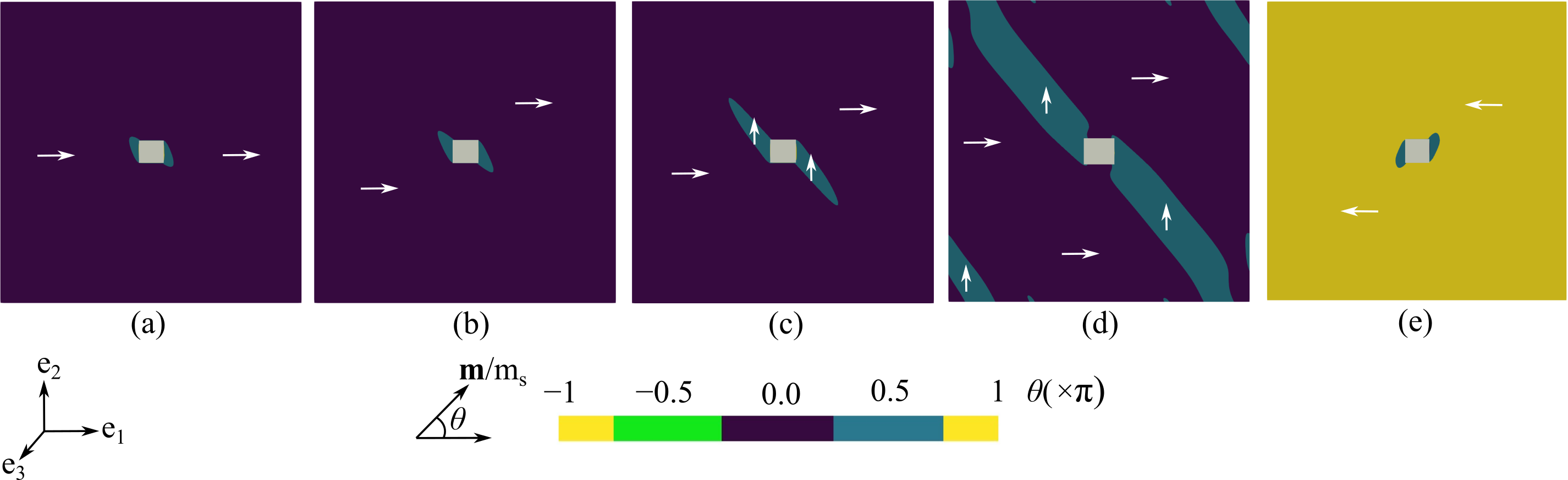
Fig. 5 shows the growth of the spike domain (localized disturbance) during magnetization reversal. A spike domain, similar to those observed in experiments [29], forms around the defect. Evidently, the growth of the spikes is driven by the energetic advantage of elimination of the poles on the (non-magnetic) defect, the decreasing influence of the applied field as it is lowered, and the tendency of the spikes to lower the contribution of the demagnetization energy of the poles at the boundary of the ellipsoid. As the applied field is lowered, the spike domain grows modestly at first, see Fig. 5(b-d). At a coercive field of Oe, the magnetization reverses abruptly. Fig. 6 shows the corresponding hysteresis and strain loops for the spike domain microstructure.
Note that, in the initial states, e.g., Fig. 5(a-c), The far-field magnetization does not change its direction as the spike domain grows. This is consistent with our arguments for the uniform magnetization in Section 2.3. As seen in Fig. 5, as the field is lowered, the spike domain grows slowly. The instability leading to the reversal is abrupt, and near complete reversal occurs everywhere except the small region surrounding the defect. The final magnetization achieved over the full ellipsoid, except very near the defect, is .

Fig. 6(a-b) shows the volume average magnetization and volume average strain of the spike domain microstructure as a function of the applied field . The labels (a-e) correspond to the subfigures in Fig. 5(a-e). In Fig. 6(a), as the external field is reduced to zero, the domain retains its net magnetization state (i.e., remnant magnetization), and no significant changes in the microstructure are observed. At the coercive field , the net magnetization reverses, and the microstructure changes drastically—for example, the spike domain grows. On reversing the direction of the applied field the magnetization switches to its initial state.
In Fig. 6(b), the volume average strain traces out a characteristic butterfly double loop that is consistent with experimental observations [12]. The strain gradually decreases as the external field is lowered, see labels (a-d), and abruptly switches at the coercive field value, label (d-e) in Fig. 6(b). At the coercive field, the magnetization in the domain reverses.
The hysteresis loop in Fig. 6(a) is square shaped with sharp shoulders near the values of the coercive field. We attribute the square shape of the hysteresis loop to the oblate ellipsoid geometry of the magnetic body—this body geometry assists in retaining a net magnetization despite reducing the external field. The sharp shoulder at result from a sudden unstable growth of the spike domain. Note that the experimentally measured coercive field value for bulk is about an order of magnitude smaller than our computed values—this may be because we assume a single crystal material with a simple defect structure and no sharp corners—and we discuss this further in Section 4. We next apply this fundamental concept of introducing a localized disturbance (spike domain) during magnetization reversal to explore the effect of stress, defect geometry and material constants on hysteresis loops.
3.2 Study 1: Effect of stress on hysteresis loops


Here, we investigate whether mechanical loads, such as tensile stress, affects coercivity in three types of magnetic alloys, namely, alloys with magnetostriction constants and . We model three magnetic disks that correspond to iron-nickel alloys with and Ni-content, respectively. We choose these specific alloy compositions because the measured magnetostriction constants for and satisfy and , respectively. The values of the other material constants corresponding to each alloy composition are listed in Table S1 of the supplementary material (Section 1). We introduce tensile loads in the micromagnetics energy via and apply stress in the range for each computational domain.
Fig. 7 shows the effect of a homogeneous macroscopic stress on hysteresis loops. The results show two key findings on the response of magnetic alloys to applied loads. First, hysteresis loops in magnetic alloys with zero magnetostriction, for example with , as expected, are unaffected by tensile loads. For example, Fig. 7(a) shows that the hysteresis loop is the same under all tensile loads . Second, the hysteresis loops in magnetic alloys with non-zero magnetostriction deviate from the hysteresis loop with zero external stress. For example, the magnetic alloy with shows an increasing coercive field with increasing tensile stress, and the magnetic alloy with shows a decreasing coercive field with increasing tensile stress. This response of the magnetic alloys is because of the coupling between the magnetostriction and the magnetization terms, for e.g., the preferred strain along direction is given by . For , the strain values are decoupled from magnetization terms, and the external loads do not affect magnetic hysteresis. Overall, Fig. 7 demonstrates that even with the modest magnetostriction constants of FeNi, applied stresses affect the width of the hysteresis loop quite significantly.
3.3 Study 2: Effect of defect geometry on hysteresis loops

In this section we investigate whether defect geometries and defect densities affect the size and shape of hysteresis loops. Fig. 8(a-c) shows computed magnetic microstructures formed around the three defect geometries. Fig. 8(d) shows the hysteresis loops for each domain configuration. Broadly, we find that coercive field increases under two conditions: First, when the defect edges are not aligned with the material’s easy axes. For example, take Fig. 8(b), in which the defect edges are inclined at angle to the easy axes. The magnetic domains formed around this defect are magnetized along the directions in order to reduce the magnetostatic energy. These domains are not aligned along the easy axes . Consequently growing these magnetized domains requires greater coercive field strength, see Fig. 8(d). Second, the coercivity increases because of a domain wall pinning effect. For example, in Fig. 8(d) the computational domain contains multiple defects that pin domain wall motion during magnetization reversal. This pinning effect gives rise to curved shoulder on the hysteresis loop and increases the coercivity of magnetic alloys, see inset Fig. 8(e). Overall, both defect geometry and defect density affect the shape and width of hysteresis loops, but the effect is surprisingly small.
In our computations, we mainly treat one defect geometry. We envisage applications to cases in which the macro-scale body is not ellipsoidal and there are multiple defects. Our studies of Fig. 8 with two defects indicate a minor effect on coercivity of having multiple defects, at least when both defects are in the small computational domain. However, a full understanding on the effects of body shape and multiple defects awaits future work. Fig. 8 and Section 3.3 of the paper do suggest that, if an array of defects were to be engineered in the direction of the spike domain, coercivity could be lowered.
3.4 Study 3: Effect of material constants on coercivity
In this section, we investigate how the interplay between a localized disturbance and magnetic material constants affects coercivity. We explore this interplay in two sub-studies: First, we model a situation relevant to the permalloy problem. We compute magnetic coercivities in the alloy system as a function of the Ni-content, see Table S2 in supplementary material (Section 1). We use magnetic material constants—namely the anisotropy and the magnetostriction constants and —as inputs and compute magnetic coercivity at each FeNi alloy composition. Second, we systematically vary the values of the anisotropy and the magnetostriction constants along the easy axes (i.e., for we vary between with , and for we vary between with ), and compute coercivities around the permalloy composition.33 3 Note that magnetic alloys with and have their easy axes along the and family of crystallographic directions, respectively. We compute the magnetic coercivities on a domain with grid points and defect of size , and by applying an external field along their respective easy axes. These calculations require a transformation of the coordinate basis that we explain in the supplementary material (Section 2).
The Permalloy problem: Fig. 9(a) shows the coercivity as a function of Ni-content in iron-nickel alloys. In line with experimental observations, the coercivity is minimum in the Ni-content range. The coercivity is the lowest at Ni-content, see Fig. 9(b). Magnetic coercivity gradually increases for material constants that lie away from the 78.5 Ni-content alloy. Fig. 9(b) shows that although at 75 Ni-content, the coercivity is not a minimum at this composition. In fact, the coercivity is minimum at 78.5 Ni-content at which neither the anisotropy constant nor the magnetostriction constants are zero. We attribute the minimum coercivity at 78.5 Ni-content to a delicate balance of the localized disturbance and material constants of the bulk alloy. We note that this balance is sensitive to the size of the defect and the presence of residual strains in the domain. Prior experimental research reports precipitate formation on cooling FeNi alloys, and we suspect that these inclusions affect the balance between material constants at , and we study this in detail in our forthcoming paper [53]. Here, we note that Fig. 9(a-b) demonstrates that magnetic material constants, such as the magnetostriction constants and the anisotropy constant, play an important role in governing hysteresis.

Parametric study: Fig. 10 shows a coercivity heat map as a function of the anisotropy constant and the magnetostriction constants . For the range of material constants explored, the coercivity is minimum when . The coercivity increases for an increase in either the anisotropy or the magnetostriction constants. The well known permalloy composition lies close to the bottom of this well in Fig. 10. However, Fig. 10 shows other combinations of material constants that have a lower coercivity than the permalloy composition. This example shows a potential use of our coercivity tool to discover novel combinations of material constants with low magnetic hysteresis. In our forthcoming papers, we investigate the interplay between , and constants to lower coercivities in iron-based magnetic alloys [52, 53].
Overall, the results in this section demonstrate two things: First, the magnetostriction constant in addition to the anisotropy constant plays an important role in reducing magnetic hysteresis. Second, the delicate interplay between a localized disturbance and material constants is a potential way forward to predicting hysteresis in bulk magnetic alloys.
4 Discussion
The results show that our coercivity tool provides a systematic framework to explore the interplay between magnetic domains and defect geometry—and how these features affect material constants that govern magnetic hysteresis. For example, in Sections 3.1–3.3 we show the growth of a spike domain during magnetization reversal, and explore the role of applied loads and defect geometry on magnetic hysteresis. Section 3.4 identifies the interplay between anisotropy and magnetostriction constants that lowers magnetic coercivity in FeNi alloys. In the remainder of this section, we discuss some limitations of our coercivity tool, and then consider some differences between our findings and prior work on predicting magnetic hysteresis.
Two features of this work limit the comparisons we can make with experimental measurements on magnetic coercivity. First, our simulations assumed the computational domains to be a single crystal with periodic boundary conditions and cubic defect geometries. While these assumptions are internally consistent and allow for detailed predictions, these idealizations are subject to the shortcomings associated with the presence of grain boundaries and a complex distribution of defects that is expected to be typical in bulk materials. From this perspective, our predictions exhibit a surprisingly favorable comparison with experiment. Second, although we predict magnetic coercivity as a function of defect geometry and material constants, the quantitative values of the coercive force are an order of magnitude greater than experimental measurements in iron-nickel alloys [35]. Whether introducing other defects, such as sharp corners, surface roughness, non-ellipsoid body geometries, into our model would yield comparable results with experiments is an open question. With these limiting conditions we next proceed to discuss strengths of our coercivity tool.
The key feature of our coercivity tool is the use of a localized disturbance in calculating the coercive force in magnetic systems. This localized disturbance is in the form of a Neel-type spike domain that introduces a non-linear variation in our numerical micromagnetics. The growth of this spike domain, under decreasing field values, destabilizes the uniformly-magnetized metastable states. Using this approach, we predict coercive field values that are much closer to experimental observations, and are more accurate than the predictions from linear stability analysis [20]. Furthermore, we numerically march through local minimizing states and trace out the characteristic hysteresis and strain loops of a magnetic alloy. These features cannot be captured using other simplifying methods based on absolute minimizers, such as the method of Gamma convergence.
Another feature of the coercivity tool is that it accounts for magneto-elastic interactions in addition to the anisotropy and magnetostatic energy terms. This rigorous formulation of the coercivity tool provides a framework to systematically explore how combinations of material constants can lower magnetic hysteresis. For example, Section 3.4 shows how both anisotropy and magnetostriction constants lower magnetic hysteresis in FeNi alloys. This finding contrasts with previous studies, in which zero anisotropy constant was considered to be the only factor that lowers magnetic hysteresis [50, 51]. Prior studies typically neglected the magnetostriction terms and their role on magnetic hysteresis was not known. Our results show that in addition to the anisotropy constant, magnetostrictive constants and play an important role in lowering magnetic hysteresis.
Beyond introducing a localized disturbance and magnetoelastic terms, the coercivity tool provides insight into nanoscale domain switching mechanisms during magnetization reversal. For example, in Section 3.1–3.3 we show the nucleation and growth mechanism of the spike-domain microstructures, and domain-wall pinning on defects under applied loads. The evolution of these microstructural features arise naturally as a result of relative energy minimization. Overall, these results demonstrate how our coercivity tool can be used to design structural features of defects, and to discover novel combinations of material constants that lower magnetic hysteresis. These results suggest initial steps for experiments and alloy development programs to design magnetic materials with low hysteresis.
5 Conclusion
The present findings contribute to a more fundamental understanding of how different variables, such as local instabilities and material constants, affect magnetic coercivity. Specifically, coercivity is often viewed to be lower in magnetic alloys with zero (or negligible) anisotropy constant, , and magnetoelastic energies are often ignored because of their small values. However, this explains little about the singularities in the permalloy problem, in which coercivity abruptly drops at a non-zero anisotropy value, Given the present findings of including both magnetoelastic and anisotropy energies to compute coercivity, we demonstrate that both magnetostrictive constants and anisotropy constants play an important role in lowering magnetic coercivity. Furthermore, we present a tool that models a large local instability (spike-domain) that lowers the coercive force necessary for magnetization reversal, and predicts coercivity with better accuracy than linear stability analysis. We propose to use this computational tool to discover a fundamental relationship between material constants that lower magnetic coercivity, and thereby develop novel magnetic systems with high anisotropy constants and low coercivity.
6 Acknowledgement
The authors acknowledge the Minnesota Supercomputing Institute at the University of Minnesota (Dr. David Porter), and the Advanced Research Computing at the University of Southern California for providing resources that contributed to the research results reported within this paper. The authors acknowledge the support of NSF (DMREF-1629026), ONR (N00014-18-1-2766). R.D.J and A.R.B, respectively, acknowledge the support of a Vannevar Bush Faculty Fellowship and a Provost Assistant Professor Fellowship. Finally, the authors thank anonymous reviewers for their insightful comments that have helped improve this manuscript.
Supplementary material
Energy of micromagnetics
In this section we describe the general form of the micromagnetics energy used in the present work. Let be the orthonormal cubic axes. We write the magnetization , position , displacement and strain tensors as follows:
| (24) |
Substituting these expressions in the micromagnetics energy, we get the free energy function:
| (25) |
Tables 1 and 2, respectively, list the values of physical and iron-nickel material constants used in our calculation.
| Physical quantities | Value | Material constants | Value | |
| Vacuum permeability, | Saturation magnetization | |||
| Gyromagnetic ratio, | Exchange energy constant | |||
| Damping constant, | Length scale | |||
| Demagnetization factors | Stiffness constants | |||
| (Oblate ellipsoid) | ||||
| Ni | (kJ/m3) | () | () | |
|---|---|---|---|---|
| 35 | 0.462 | -5.85 | 16.9 | 0.94 |
| 38 | 0.889 | -7.30 | 25.5 | 1.13 |
| 42 | 1.140 | -3.89 | 32.3 | 1.23 |
| 45 | 1.100 | 0.0 | 32.8 | 1.26 |
| 50 | 0.958 | 10.0 | 30.9 | 1.25 |
| 55 | 0.847 | 20.9 | 26.8 | 1.19 |
| 60 | 0.701 | 26.2 | 22.2 | 1.15 |
| 65 | 0.500 | 25.6 | 16.5 | 1.07 |
| 70 | 0.287 | 22.3 | 10.7 | 0.99 |
| 73 | 0.142 | 18.9 | 7.13 | 0.94 |
| 74 | 0.052 | 18.5 | 6.29 | 0.92 |
| 75 | 0.000 | 17.2 | 5.46 | 0.90 |
| 77 | -0.084 | 14.5 | 3.68 | 0.87 |
| 78.5 | -0.161 | 11.8 | 1.91 | 0.84 |
| 80 | -0.273 | 8.45 | 0.0 | 0.82 |
| 83 | -0.520 | 0.0 | -2.68 | 0.76 |
| 90 | -1.600 | -23.2 | -10.8 | 0.64 |
| 100 | -5.880 | -53.1 | -26.5 | 0.48 |
Magnetic alloys with
In this section we describe the general form of the micromagnetics energy for magnetic ellipsoids with . Magnetic alloys with have the easy axes along the family of crystallographic directions. In order to compute magnetic coercivity along the easy axes, we model magnetic ellipsoids such that the crystallographic direction lies in the plane of the ellipsoid and along the ellipsoid’s major axis. Specifically, we model magnetic ellipsoids with crystallographic directions and in-plane, and apply an external field along the direction. We next transform the coordinate basis, and write the free energy of micromagnetics in this transformed basis.
Let the orthonormal basis represent the crystallographic directions along , and , respectively. The orthonormal cubic basis is related to the transformed bases as follows:
Or, more relevant,
| (35) |
We write the magnetization , position , displacement and strain tensors in the inclined basis as follows:
| (36) |
Substituting for the basis and the tensors in the micromagnetics energy, we have:
| (37) |
Ellipsoids and demagnetization fields
This section shows how we simplify the demagnetization energy of a localized, perturbed magnetization caused by a nonmagnetic defect inside a ferromagnetic ellipsoid. The result is that the demagnetization energy, including both the long range effect of the poles at the boundary of the ellipsoid and the localized perturbation, is given by an explicit expression. Using a small localized simulation, this result allows us to include the effect of a surrounding ellipsoid that is much larger than the defect (e.g., the effect of poles on far-away boundaries) on the magnetization distribution near the defect and on the total demagnetization energy. Without this simplification we would have also to compute the magnetization and magnetic field on the full magnetic body, and also the decaying field outside the magnetic body, to sufficient accuracy.
Let a magnetization be supported on an ellipsoidal region . The magnetic field is and the magnetostatic equation is div, or, in weak form,
| (38) |
which is to be solved for functions , that is, square integrable functions with square integrable gradients on all of space. It is known that the solution , of (38) in this sense is unique. Here, on and, for the purpose of solving (38), is taken to be zero outside . The magnetostatic energy is
| (39) |
These various forms are obtained by using (38) with . We will use several known tricks to simplify the calculation. These are:
- 1.
Since is an ellipsoid, the magnetic field produced by a constant magnetization is constant on the ellipsoid and is given by
(40) The demagnetization matrix is a (tabulated) purely geometric property of the ellipsoid and is coaxial with its principal axes. Of course, is not constant outside . The corresponding magnetostatic energy of this magnetization is
(41) - 2.
There is a reciprocal theorem, which is proved in the standard way by writing (38) for a magnetization “a” and choosing the magnetostatic potential for “b”, then writing (38) for “b” and choosing as the potential for “a”, and subtracting:
(42) (Note that and do not have to be supported on the same domain.)
We use the above observations to calculate the demagnetization energy due to the presence of a nonmagnetic defect. We decompose
| (43) |
Let be the field due to the perturbation: div.
This defect occupies a region . The argument does not actually assume is small, but the result is useful for simulation in that case. In that case the perturbed magnetization is expected to be supported on a computational region . Note that if is defined by a tolerance, it scales linearly with (i.e., ) by the scaling law of the magnetostatic equation, so it shrinks to zero as the defect shrinks to zero.
Since is an ellipsoid, the field of the constant magnetization on all of is on , and its magnetostatic energy is
| (44) |
By the linearity of the magnetostatic equation, the total magnetization produces the magnetic field . The total magnetostatic energy is
| (45) | |||||
Since is given by a simple expression, we use the reciprocal theorem to replace the third term by the second and we also introduce Eq. (44):
| (46) | |||||
| (47) |
Next we reintroduce in order to impose the constraint .
| (48) | |||||
| (49) | |||||
| (50) |
Note that should be near zero at because there is no dipole term due to . Eq. (50) is the form of magnetostatic energy that we use in the present work.
Computing equilibrium equations in Fourier space
Following Zhang and Chen [33], we solve the magnetostatic equilibrium equation Eq. 5 and the elastic equilibrium equations Eq. 3 in Fourier space. For example, the magnetostatic equilibrium equation in Fourier space is given by:
| (51) |
Here, are the coordinates in Fourier space and are Fourier transforms of the magnetostatic potential and the magnetization , respectively. The magnetostatic potential is computed at each iteration as:
| (52) |
Similarly, we solve the mechanical equilibrium equation Eq. 3 in Fourier space. First, we define the total strain tensor as a sum of the homogeneous and heterogeneous strains , i.e., The homogeneous strain is a constant and corresponds to the average deformation of the computational domain. This strain is computed as follows:
| (53) |
Here, is a simple volume average of the th magnetization component in the computational domain. In the presence of external loads, such as a homogeneous macroscopic stress , the homogeneous strain is computed as . Here, is the compliance tensor of the magnetic alloy.
The heterogeneous strain is a symmetric tensor . The general solution of the displacement field is given by:
| (54) |
This solution in Fourier space reduces to:
| (55) |
where and is the Fourier transform the spontaneous strain tensor. The expression computes the inverse of the stiffness matrix in Fourier space. That is, is a matrix with elements , and and are the co-factors and determinant of the matrix . We next reproduce the calculated expressions in Zhang and Chen [33], for the co-factors and determinant of the matrix for cubic crystals:
| (56) |
in which,
| (57) |
The other components of the co-factors are obtained by cyclical permutation of 1,2,3. In our computations, we solve both magnetostatic and elastic equilibrium equations at every time step. Although, we solve these equations in Fourier space these computations get expensive for larger domain sizes. Following Bozorth’s analytical calculation for domain wall thickness (Chapter 8, Ref. [22]), we choose a grid size of nm, such that domain walls span across at least four elements.
The presence of a nonmagnetic defect introduces discontinuities in magnetization. While the magnetization itself flows smoothly around the defect (e.g., see Fig. 5 and Fig. 8) and satisfies the jump conditions in Eqs. 10-12 (main text), care is needed to resolve magnetization during Fourier transformation. We implement our model in a code and use the “Fastest Fourier Transform in the West” (FFTW) library. We use this library to compute the discrete Fourier transform, of both real and complex data, in three dimensions. In the FFTW implementation of the discrete Fourier transform the input length of the data () determines the total number of frequencies (i.e., frequency range) of the Fourier transform. In our computations we use a broad frequency range (e.g., in Fig. 5 (main text) we use a frequency range containing about samples) to sufficiently resolve the change in magnetization around the defect. For example, assume a sharp jump in the magnetization near the defect. Our calculations show that this discontinuity in magnetization is sufficiently resolved with a frequency range of 40 samples, but is well resolved at higher frequencies (e.g., and ). While such a sharp jump in magnetization is unlikely to occur in our computations because the gradient energy term in Eq. (1) (of main text) penalizes abrupt changes in magnetization leading to a diffuse interface (e.g., domain wall). In our computations, these domain wall spans across 3-4 elements, which is similar to those in previous magnetic calculations (e.g., [32, 33]). In these cases, our frequency range of sufficiently resolves discontinuities in magnetization on the computational domain.
By solving these equations in Fourier domain and by using FFTW we improve the computational efficiency of our algorithm by [57]. A key reason for this computational efficiency is because we transform the differential equations in real space (in Eqs. 3-5 and Eqs. 7-9) to algebraic equations in Fourier space. These algebraic equations are easier to compute and therefore improves the computational efficiency of our tool. Furthermore, the FFTW library uses the Cooley-Tukey algorithm which uses a recursive strategy that contributes to the computational speed [58]. Further details on the FFTW libraries and the Cooley-Tukey algorithm can be found in these Refs. [57, 58].
The computational efficiency of the coercivity tool becomes evident in our subsequent calculations, e.g., Fig. 10. In these parametric calculations, we compute coercivities on individual domains with different material constants. These computations are feasible and inexpensive because of the computational efficiency achieved by solving the governing equations in Fourier space.
Gauss-Siedel Projection Method in Fourier space
We employ the Gauss-Siedel projection method developed by Wang et al. [32] to numerically solve the Landau-Lifshitz-Ginzburg equation Eq. 6. The effective field is defined as the variational derivative of the free energy function with respect to the magnetization :
| (58) |
Here, is the first variation of the free energy function with respect to the magnetization, excluding the exchange energy. Substituting for the effective field in the Eq. 6, we have:
| (59) |
The key steps followed in solving Eq. 59 using the Gauss-Siedel projection method are described in Section 2.4 (Eq. 7–9). Next, we describe how Eqs. 7–9 are solved in Fourier space.
For example, we compute Eq. 7 in Fourier space and solve for the intermediate fields at the th time step as follows:
| (60) |
in which is the Fourier transformation of the field . Similarly, we compute the intermediate magnetization in Fourier space as:
References
- [1] Gutfleisch, O., Willard, M. A., Brück, E., Chen, C. H., Sankar, S. G., & Liu, J. P. (2011). Magnetic materials and devices for the 21st century: stronger, lighter, and more energy efficient. Advanced materials, 23(7), 821-842.
- [2] Jiles, D. C. (2003). Recent advances and future directions in magnetic materials. Acta materialia, 51(19), 5907-5939.
- [3] James, R. D. (2015). Materials science: Magnetic alloys break the rules. Nature, 521(7552), 298-299.
- [4] Garcıa-Otero, J., Porto, M., Rivas, J., & Bunde, A. (1999). Influence of the cubic anisotropy constants on the hysteresis loops of single-domain particles: A Monte Carlo study. Journal of applied physics, 85(4), 2287-2292.
- [5] Kachkachi, H., & Dimian, M. (2002). Hysteretic properties of a magnetic particle with strong surface anisotropy. Physical Review B, 66(17), 174419.
- [6] Herzer, G. (2005). Anisotropies in soft magnetic nanocrystalline alloys. Journal of Magnetism and Magnetic Materials, 294(2), 99-106.
- [7] Bozorth, R. M. (1953). The permalloy problem. Reviews of Modern Physics, 25(1), 42.
- [8] Lewis, B. (1964). The permalloy problem and magnetic annealing in bulk nickel-iron alloys. British Journal of Applied Physics, 15(4), 407.
- [9] Takahashi, M., Nishimaki, S., & Wakiyama, T. (1987). Magnetocrystalline anisotropy and magnetostriction of Fe-Si-Al (Sendust) single crystals. Journal of magnetism and magnetic materials, 66(1), 55-62.
- [10] Shih, J. W. (1934). Magnetic properties of iron-cobalt single crystals. Physical Review, 46(2), 139.
- [11] Li, G. P., Wang, J., Shimada, T., Fang, H., & Kitamura, T. (2014). Strain-induced polarity switching of magnetic vortex in alloys with different compositions. Journal of Applied Physics, 115(20), 203911.
- [12] Bozorth, R. M. (1993). Ferromagnetism (p. 992).
- [13] Brown, W. F. (1962). Magnetostatic Principles in Ferromagnetism. In: Selected Topics in Solid State Physics. Vol. 1. Ed. by E. P. Wohlfahrt. North-Holland.
- [14] Slonczewski, J. C. (1956). Theory of magnetic hysteresis in films and its applications to computers. Research Memo RM 003.111.224, IBM Research Center.
- [15] Aharoni, A., & Shtrikman, S. (1958). Magnetization curve of the infinite cylinder. Physical Review, 109(5), 1522.
- [16] Brown Jr, W. F. (1957). Criterion for uniform micromagnetization. Physical Review, 105(5), 1479.
- [17] Aharoni, A. (1963). Complete eigenvalue spectrum for the nucleation in a ferromagnetic prolate spheroid. Physical Review, 131(4), 1478.
- [18] Shiratsuchi, Y., Yamamoto, M., & Bader, S. D. (2007). Magnetism and surface structure of atomically controlled ultrathin metal films. Progress in surface science, 82(2-3), 121-160.
- [19] Landau, L. D. & Lifshitz, E. M. Physik. Z. Sowjetunion 8 (1935), 337-346
- [20] Brown Jr, W. F. Micromagnetics (1963). John Wiley & Sons. S06 Wednesday, March, 25(14), 40-15.
- [21] Brown, W. F. (1966). Magnetoelastic interactions (Vol. 9). Berlin: Springer.
- [22] Bozorth, R. M. (1993). Ferromagnetism, by Richard M. Bozorth, pp. 992. ISBN 0-7803-1032-2. Wiley-VCH, August 1993., 992.
- [23] James, R. D., & Zhang, Z. (2005). A way to search for multiferroic materials with “unlikely" combinations of physical properties. In Magnetism and structure in functional materials (pp. 159-175). Springer, Berlin, Heidelberg.
- [24] Zhang, Z., James, R. D., & Muller, S. (2009). Energy barriers and hysteresis in martensitic phase transformations. Acta Materialia, 57(15), 4332-4352.
- [25] Zarnetta, R., Takahashi, R., Young, M. L., Savan, A., Furuya, Y., Thienhaus, S., Maaß, B., Rahim, M., Frenzel, J., Brunken, H., & Chu, Y. S. (2010). Identification of quaternary shape memory alloys with near-zero thermal hysteresis and unprecedented functional stability. Advanced Functional Materials, 20(12), 1917-1923.
- [26] Cui, J., Chu, Y. S., Famodu, O. O., Furuya, Y., Hattrick-Simpers, J., James, R. D., Ludwig, A., Thienhaus, S., Wuttig, M., Zhang, Z. & Takeuchi, I. (2006). Combinatorial search of thermoelastic shape-memory alloys with extremely small hysteresis width. Nature materials, 5(4), 286-290.
- [27] Pilet, N. (2006). The relation between magnetic hysteresis and the micromagnetic state explored by quantitative magnetic force microscopy (Doctoral dissertation, University of Basel).
- [28] Néel, L. (1944). Effet des cavités et des inclusions sur le champ coercitif, Cahiers de Physique 25, 21-44.
- [29] Williams, H. J. (1947). Direction of domain magnetization in powder patterns. Physical Review, 71(9), 646.
- [30] Hubert, A., & Schäfer, R. (2008). Magnetic domains: the analysis of magnetic microstructures. Springer Science & Business Media.
- [31] James, R. D., & Kinderlehrer, D. (1990). Frustration in ferromagnetic materials. Continuum Mechanics and Thermodynamics, 2(3), 215-239.
- [32] Wang, X. P., Garcıa-Cervera, C. J., & Weinan, E. (2001). A Gauss–Seidel projection method for micromagnetics simulations. Journal of Computational Physics, 171(1), 357-372.
- [33] Zhang, J. X., & Chen, L. Q. (2005). Phase-field microelasticity theory and micromagnetic simulations of domain structures in giant magnetostrictive materials. Acta Materialia, 53(9), 2845-2855.
- [34] Landis, C. M. (2008). A continuum thermodynamics formulation for micro-magneto-mechanics with applications to ferromagnetic shape memory alloys. Journal of the Mechanics and Physics of Solids, 56(10), 3059-3076.
- [35] Bozorth, R. M. (1993). Ferromagnetism. Ferromagnetism, by Richard M. Bozorth, pp. 992. ISBN 0-7803-1032-2. Wiley-VCH, August 1993., 992.
- [36] Dabade, V., Venkatraman, R., & James, R. D. (2019). Micromagnetics of galfenol. Journal of Nonlinear Science, 29(2), 415-460.
- [37] Scheinfein, M. R., Unguris, J., Blue, J. L., Coakley, K. J., Pierce, D. T., Celotta, R. J., & Ryan, P. J. (1991). Micromagnetics of domain walls at surfaces. Physical Review B, 43(4), 3395.
- [38] Knüpfer, H., Kohn, R. V., & Otto, F. (2013). Nucleation barriers for the cubic-to-tetragonal phase transformation. Communications on pure and applied mathematics, 66(6), 867-904.
- [39] Knüpfer, H., & Otto, F. (2019). Nucleation barriers for the cubic-to-tetragonal phase transformation in the absence of self-accommodation. ZAMM-Journal of Applied Mathematics and Mechanics (Zeitschrift für Angewandte Mathematik und Mechanik) 99(2), e201800179.
- [40] Hestenes, M.R. (1948). Sufficient conditions for multiple integral problems in the calculus of variations. American J. Math. 70, 239-276.
- [41] Campos Cordero, J. (2017). Boundary regularity and sufficient conditions for strong local minimizers. J. Functional Analysis 272, 4513-4587.
- [42] Y. Grabovsky, Y & Mengesha, T. (2009). Sufficient conditions for strong local minima: the case of C1 extremals, Trans. Amer. Math. Soc. 361(3), 1495-1541.
- [43] Horgan, C. O. (1995). Korn’s inequalities and their applications in continuum mechanics. SIAM review, 37(4), 491-511.
- [44] Landau, L. A. & Lifshitz, E. (1992). On the theory of the dispersion of magnetic permeability in ferromagnetic bodies. In Perspectives in Theoretical Physics (pp. 51-65). Pergamon.
- [45] Gilbert, T. L. (2004). A phenomenological theory of damping in ferromagnetic materials. IEEE transactions on magnetics, 40(6), 3443-3449.
- [46] Bruckner, F., Vogler, C., Bergmair, B., Huber, T., Fuger, M., Suess, D., Feischl, M., Fuehrer, T., Page, M. & Praetorius, D., (2013). Combining micromagnetism and magnetostatic Maxwell equations for multiscale magnetic simulations. Journal of magnetism and magnetic materials, 343, 163-168.
- [47] Praetorius, D., Ruggeri, M., & Stiftner, B. (2018). Convergence of an implicit-explicit midpoint scheme for computational micromagnetics. Computers & Mathematics with Applications, 75(5), 1719-1738.
- [48] Lakshmanan, M. (2011). The fascinating world of the Landau-Lifshitz-Gilbert equation: an overview. Philosophical Transactions of the Royal Society A: Mathematical, Physical and Engineering Sciences, 369, 1280-1300.
- [49] Veligatla, M., Titsch, C., Drossel, W. G., Garcia-Cervera, C. J., & Müllner, P. (2020). Sensitivity of twin boundary movement to sample orientation and magnetic field direction in Ni-Mn-Ga. Acta Materialia, 186, 389-395.
- [50] Herzer, G. (1995). Soft magnetic nanocrystalline materials. Scripta Metallurgica et Materialia, 33(10-11), 1741-1756.
- [51] Fiorillo, F. (2006). Anisotropy and magnetization process in soft magnets: Principles, experiments, applications. Journal of magnetism and magnetic materials, 304(2), 139-144.
- [52] Renuka Balakrishna, A. & James, R.D. (Preprint 2020). A search for magnetic alloys with low hysteresis. Available on request.
- [53] Renuka Balakrishna, A. & James, R.D. (Preprint 2020). A solution to the permalloy problem. Available on request.
- [54] Bozorth, R. M. & Walker, J. G. (1953). Magnetic crystal anisotropy and magnetostriction of iron-nickel alloys. Physical Review, 89(3), 624.
- [55] Cullity, B. D., & Graham, C. D. (2011). Introduction to magnetic materials. John Wiley & Sons.
- [56] Liu, L., James, R. D., & Leo, P. H. (2007). Periodic inclusion-matrix microstructures with constant field inclusions. Metallurgical and Materials Transactions A, 38(4), 781-787.
- [57] Frigo, M., & Johnson, S. G. (2005). The design and implementation of FFTW3. Proceedings of the IEEE, 93(2), 216-231.
- [58] Cooley, J. W., & Tukey, J. W. (1965). An algorithm for the machine calculation of complex Fourier series. Mathematics of computation, 19(90), 297-301.