Planar Maximum Coverage Location Problem with Partial Coverage, Continuous Spatial Demand, and Adjustable Quality of Service
Manish Bansal and Parshin Shojaee
Department of Industrial and Systems Engineering, Virginia Tech
Email: bansal@vt.edu, parshinshojaee@vt.edu
First Draft: December 10, 2020
Abstract. We consider a generalization of the classical planar maximum coverage location problem (PMCLP) in which partial coverage is allowed, facilities have adjustable quality of service (QoS) or service range, and demand zones and service zone of each facility are represented by two-dimensional spatial objects such as rectangles, circles, polygons, etc. We denote this generalization by PMCLP-PC-QoS. A key challenge in this problem is to simultaneously decide position of the facilities on a continuous two-dimensional plane and their QoS. We present a greedy algorithm and a pseudo-greedy algorithm for it, and showcase that the solution value corresponding to the greedy (or pseudo-greedy) solution is within a factor of (or ) of the optimal solution value where is the base of natural logarithm and . We also investigate theoretical properties and propose exact algorithms for solving: (1) PMCLP-PC-QoS where demand and service zones are represented by axis-parallel rectangles (denoted by PMCLP-PCR-QoS), which also has applications in camera surveillance and satellite imaging; and (2) one dimensional PMCLP-PC-QoS which has applications in river cleanups. These results extend and strengthen the only known exact algorithm for PMCLP-PCR-QoS with fixed and same QoS by Bansal and Kianfar [INFORMS Journal on Computing 29(1), 152-169, 2017]. We present results of our computational experiments conducted to evaluate the performance of our proposed exact and approximation algorithms.
Keywords: planar maximum coverage location problem; partial coverage; adjustable quality of service; greedy approach; spatial demand representation; branch-and-bound exact algorithm
1 Introduction
Over the years, many classes of problems related to locating service facilities to cover the demand for service have been studied; refer to Church and Murray 2013, Drezner and Hamacher 2002 for extensive reviews. A well-known classical facility location problem is Maximum Coverage Location Problem (MCLP) for locating service facilities having known service range with the objective of maximizing the total covered demand (Church and ReVelle 1974). In literature, various forms of MCLP consider a finite set of pre-determined candidate positions for the facilities (Church and ReVelle 1974, Murray and O’Kelly 2002, Daskin et al. 1989). However, a generalization of the classical MCLP, referred to as the planar MCLP (PMCLP), considers locating the facilities anywhere in a continuous two-dimensional plane (Church 1984, Watson-Gandy 1982, Mehrez and Stulman 1982). These problems have received considerable attention in the literature due to their widespread applicability ranging from locating emergency healthcare centers, locating fire fighting stations, and making policy through geographical informative systems (GIS) to solve clustering problems which themselves find applications in data mining, machine learning, and bio-informatics (Chung 1986, Farahani et al. 2012, Schilling et al. 1993). With the growing availability of spatial data in the foregoing domains, the state-of-the-art facility location analytical tool set needs to evolve. In this paper, we consider a generalization of the PMCLP, by utilizing spatial representation of demand and service zones of facilities, allowing adjustable quality of service (QoS) or service range for the facilities, and allowing partial coverage in its true sense.
In most of the PMCLP literature, demands are represented as aggregated points, which are obtained by aggregating the demand of each zone at a single representative point (e.g., its centroid). Murray and Tong 2007 considered PMCLP where the demand zones are represented as line segments or polygons instead of limiting them to be represented by aggregated points. However, similar to the PMCLP with point representation of demand, they assume that demand zones (points, line segments, or polygons) are either completely covered or not covered at all by any service zone. This coverage assumption is referred to as “binary coverage” (Bansal and Kianfar 2017). The binary coverage is a simplifying assumption to model PMCLP as binary programs, but it ignores partial coverage of demand zones. Researchers have studied its impact and referred to it as region misrepresentation coverage error (RMCE) (Current and Schilling 1990, Tong and Church 2012, Murray 2016). These analysis represent that the modeling solutions are sensitive to how demand is represented in the PMCLP (Murray and O’Kelly 2002), and there are evidences that the point representation introduces unintended measurement and interpretation errors (Current and Schilling 1990, Tong and Murray 2009) which lead to gaps in actual coverage.
In Figure 1(a), we present an example of PMCLP where demand zones are represented using points and the service zone of a facility with fixed service range , using Euclidean distance, is a circle of radius centered at the facility. Observe that because of the binary coverage assumption, only two demand zones are completely covered by the service zone, whereas others are not at all covered. This causes RMCE because in reality, as shown in 1(b), five demand zones (represented by spatial objects) are partially covered by the service zone. Note that the service zone of a facility, using the rectilinear distance, is a diamond (a square rotated degrees) with a diagonal of centered at the facility. Lately, Bansal and Kianfar 2017 developed the first exact algorithm for the PMCLP where “partial coverage” is allowed, and service and demand zones are defined by axis-parallel rectangles. It generalizes PMCLP with rectilinear distance. However, they assumed that all facilities have fixed and same service range or QoS, i.e., dimensions of the rectangular service zones are fixed and same.
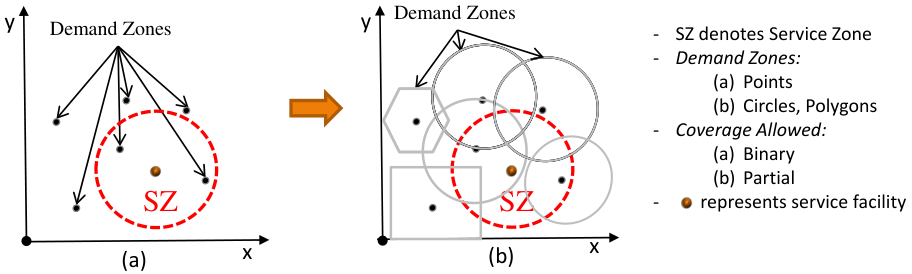
Although attempts have been made to separately address non-point representation of demand, partial coverage, and adjustable QoS, but to our knowledge, no study has tackled them together. Few studies have considered MCLP with gradual coverage, i.e., the coverage level of a demand zone depends on their distance from the facilities (Berman and Krass 2002, Church and Roberts 1983, Berman et al. 2003), but similar to MCLP, the demand zones are still represented by points and there is a finite set of pre-specified candidate positions for the facilities. This problem is referred to as gradual coverage location problem. Drezner et al. 2004 considered planar version of the forgoing problem with only single facility. (See section 2 for more details.) However so far, no study has considered PMCLP with () general representation of demand and service zones using two-dimensional spatial objects, () facilities having adjustable QoS or service range, and () partial coverage in its true sense, i.e., when covering only part of a demand zone is allowed and the coverage accrued in the objective function as a result of this is proportional to the demand of the covered area only. We denote this generalization of PMCLP by PMCLP-PC-QoS.
1.1 Problem definition: PMCLP-PC-QoS
We define the PMCLP-PC-QoS as follows. Let be a set of (possibly overlapping) spatial objects, referred to as demand zones (DZs), on a two-dimensional plane such that dimensions and location of each DZ are known. Now, consider another set of spatial objects that provide coverage of facilities, referred to as service zone (SZ), and denote the set of SZs by . We assume that shape and orientation of all SZs are same and known, but their location and dimensions are unknown. Let be a spatial object with same shape and orientation as of the SZs, but with known dimensions. We refer to as “base” SZ because it provides base reward rate (per unit area) for covering each DZ . Dimensions of each SZ is a scalar multiple of the dimensions of . We refer to as the scaling factor of SZ . The base reward rate is utilized to compute the reward rate for each DZ covered by a SZ with scaling factor , where is a strictly increasing function. When scaling factor increases, the dimensions of a SZ increases but the corresponding reward rate decreases. Therefore, by increasing the scaling factor , the service range of a facility increases, but the QoS decreases. We assume that is a finite set of possible scaling factors for SZ , which allows adjustable QoS for the SZs. In this paper, we will use terms QoS, scaling factor, or service range interchangeably for a SZ and associate all of them with for .
The goal of PMCLP-PC-QoS is to identify the location and QoS of all SZs, i.e., for all , where denotes coordinates of either center or a corner (if exists) of SZ . The objective function of this problem is to maximize the total reward captured by these SZs, i.e.,
| (1) |
where and denote the union and intersection of coverage zones, returns the total reward captured from DZ by SZs , and . In case each SZ offers same QoS, i.e., for all , the function reduces to where returns the area of its argument. In this paper, we present greedy and pseudo-greedy approximation algorithms for the PMCLP-PC-QoS as well as exact algorithms for its following variants:
(a) PMCLP-PC-QoS with axis-parallel rectangular service and demand zones (denoted by PMCLP-PCR-QoS). Given a set of rectangular DZs identified by coordinates of their lower left corner and their dimensions (width and length), denoted by and , respectively, for . We assume that the base SZ is an axis-parallel rectangle with width and length . Consequently, the SZs are also axis-parallel rectangles. We also assume that the set of scaling factors, for all . The goal of PMCLP-PCR-QoS is to find locations () as well as scaling factor of all SZ such that the maximum reward is covered. Observe that the width and length of SZ depend on the scaling factor associated to it, i.e., . A motivation behind studying this problem is its application in telerobotics, camera surveillance, and satellite imaging (refer to the next section for details). Also, the problems studied by Song et al. 2006 and Bansal and Kianfar 2017 are special cases of PMCLP-PCR-QoS where and , i.e., the facilities cannot adjust QoS and their SZs have fixed and same dimensions, respectively. Bansal and Kianfar 2017 also proved that if is a part of input, PMCLP-PCR-QoS with , denoted by PMCLP-PCR, is NP-hard. Therefore, PMCLP-PC-QoS and PMCLP-PCR-QoS are also NP-hard because PMCLP-PCR is a special case of these problems.
(b) One-dimensional PMCLP-PC-QoS (1D-PMCLP-PC-QoS): As the name suggests, the one-dimensional facility location problem has DZs and SZs placed on a line. Specifically, we assume that the DZs are line segments on -axis whose coordinate of left corner or end point, , , and width, , , are known. Likewise, the SZs are also defined as line segments on -axis with different QoS, i.e., . The motivation behind studying this special case is its application in locating trash booms (facilities) for cleaning trash zones (or DZs) in a river (represented by 1D line). In the next section, we discuss more about this application as well. Another application of this problem is in locating regional wastewater treatment plants on a river that has a given set of fixed segments (DZs) with high priority (reward rate). To our knowledge, the 1D-PMCLP-PC-QoS has not been studied before. In literature, one-dimensional plant location problem is studied by Brimberg and ReVelle 1998, and Brimberg et al. 2001 where DZs are represented by points, and facilities are uncapacitated and capacitated, respectively. As a result, the authors were able to provide mixed binary programs and dynamic programs, respectively, for them. They also show that under certain conditions, these problems are polynomially solvable using linear programs.
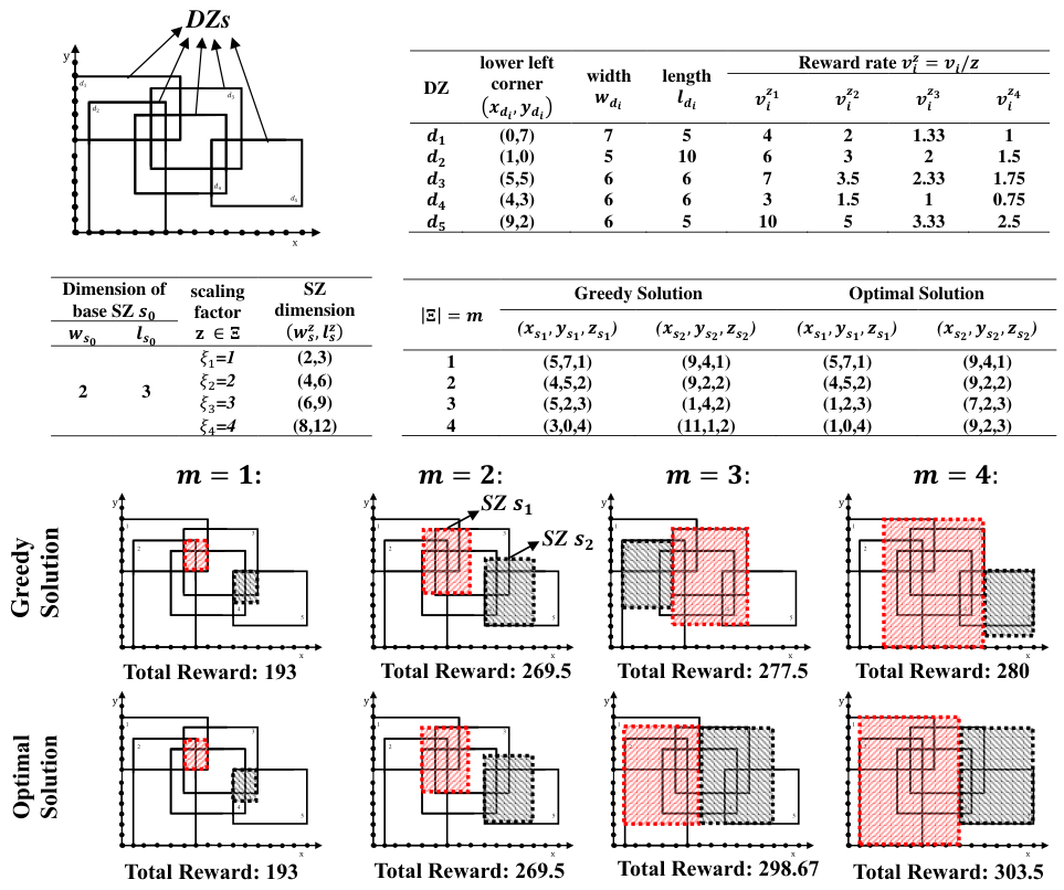
In Figure 2, we provide an example to illustrate PMCLP-PCR-QoS with five DZs with known location, width, length, and base reward rates, a base SZ with known dimensions, and a set of scaling factors for two SZs, i.e. . A similar example for has been considered by Bansal and Kianfar 2017. The locations and dimensions are considered integers just for the simplicity of representation. In this example, we assume that and therefore, . Using the algorithms presented in this paper, we present optimal and greedy solutions (along with solution values, i.e., reward) for and , . Notice that for , the greedy solution is same as the optimal solution for this example. However, for , the optimal solution value is better than the greedy solution value. Moreover, with the increase in , the captured reward is non-decreasing because the solution space for smaller value of is a subset of solution space for larger value of . This demonstrates a significance of considering facilities with adjustable QoS.
1.2 Other Applications of the PMCLP-PC-QoS
The PMCLP-PC-QoS also has direct applications in variety of emerging domains:
(a) Telerobotics. The advent of network-based telerobotic camera systems enable multiple participants or researchers in space exploration, health-care, and distance learning, to interact with a remote physical environment using shared resources. This system of networked robotic cameras with discrete resolutions receives rectangular requests or subregions (DZs) from multiple users for monitoring (Song et al. 2006, Xu et al. 2010, Xu et al. 2008). Each request has an associated reward rate (per-unit area) that may depend on the priority of the user or the importance level associated with monitoring that subregion and the resolution level (QoS) of the camera utilized to cover the subregion. The goal is to select the best view frame for the cameras (rectangular SZs) and their resolution (QoS) to maximize the total reward from the captured parts of the requested subregions. Interestingly, this problem is same as the PMCLP-PCR-QoS. In the literature, Song et al. 2006 studied the PMCLP-PCR-QoS for single camera, i.e. , and Xu et al. 2010, Xu et al. 2008 considered the PMCLP with rectangular DZs and binary coverage where the rectangular SZs are not allowed to overlap. The PMCLP-PCR-QoS subsumes the foregoing problems.
(b) River Cleaning. The main motivation behind studying the 1D-PMCLP-PC-QoS is its application in locating trash-booms for river cleanup. Rivers are the primary recipient of stormwater and as a result, the amount of trash, floating debris, and litter in them is rapidly increasing. The major sources along the river that contribute to the trash problem include industrial and recreational parks, and tributaries. There are numerous on-going efforts to clean rivers in the US and also across the globe, for example, Nile in Egypt, Yangtze in China, Ganga in India, etc. One way to reduce/cover trash in rivers is by appropriately locating trash-booms in and along the rivers. Since the point representation of a trash zone does not take into account the displacement of the trash from source locations. Therefore, an analogous of 1D-PMCLP-PC-QoS is a trash-boom location problem, where a river is represented by a one-dimensional axis, and trash zones (or DZs) and coverage of trash-booms (SZs) are represented by line segments. In this problem, the service range of each trash boom is known but can be different, and the partial coverage is allowed.
1.3 Organization of this Paper
In Section 2, we discuss challenges in solving PMCLP-PC-QoS using well-known approaches for solving (planar) MCLP and its variants. We present a greedy algorithm and a pseudo-greedy algorithm for solving the PMCLP-PC-QoS (Section 3), and showcase that the solution value corresponding to the greedy solution is within a factor of of the optimal solution value where is the base of natural logarithm. This extends the similar results of Cornuéjols et al. 1977 and Hochbaum and Pathria 1998 for special cases of PMCLP-PC-QoS (see Section 2.2 for details). In Section 4, we analyze the objective function and solution space of the PMCLP-PCR-QoS. We strengthen the theoretical properties provided for PMCLP-PCR in Bansal and Kianfar 2017 by reducing the solution search space and thereby, improve the computational efficiency of their algorithm. We also introduce theoretical properties to reduce search space for optimal solution of PMCLP-PCR-QoS, and utilize these properties to develop a branch-and-bound based exact algorithm for it. In Section 5, we introduce 1D-PMCLP-PC-QoS and provide theoretical properties for its solution space along with an exact algorithm for it. We also conduct computational experiments to evaluate the performance of our exact algorithms and greedy approach for PMCLP-PCR, PMCLP-PCR-QoS, and 1D-PMCLP-PC-QoS (Section 6). Finally, we provide our concluding remarks in Section 7.
2 Challenges in solving PMCLP-PC-QoS
In this section, we present two well-known approaches for solving (planar) MCLP and its variants, and discuss how they cannot be directly utilized for solving the PMCLP-PC-QoS.
2.1 Linear Binary Programming
The motivation for the binary coverage assumption in the (planar) MCLP (where demand is represented by points, line segments, or polygons) is to make the problem manageable by readily formulating them as a linear binary program (LBP). This is easy to do for the MCLP because of the discrete nature of candidate locations for service facilities (as per the definition). Moreover, even in studies considering a planar setting, i.e., allowing the facilities to be located anywhere in the continuous plane, coverage is still assumed to be binary (Murray and Tong 2007) because this helps to show that a finite number of potential facility locations, called the circle intersection point set (CIPS) (Church 1984) and polygon intersection point set (PIPS) (Murray and Tong 2007), exist which contain an optimal solution to this problem. Thereby resulting in the following well-known LBP for the (planar) MCLP:
| (2) |
where binary variable if demand zone is covered and otherwise, variable if a service facility is sited at the candidate/PIP/CIP point and otherwise, is the given total demand of demand zone , and is the given binary value which is 1 if demand zone is covered by locating a facility at candidate/CIP/PIP point , i.e., distance between point is no greater than known service range of a facility (denoted by ) located at point or .
Furthermore in literature, LBP formulations have also been used to tackle so-called gradual coverage location problem (GCLP). Similar to the MCLP, in GCLP, the demand zones are still represented by points but the coverage level depends on their distance from the facilities. So far LBP formulations are known only for the GCLP defined over a finite set of pre-specified candidate positions for the facilities (Berman and Krass 2002, Berman et al. 2003, Church and Roberts 1983), and planar GCLP with single facility, i.e. (Drezner et al. 2004). More specifically, given a set of demand points and a set of finite number of positions where facilities can be placed, the GCLP can be stated as follows: where is a set of locations where facilities are located, is the minimum distance between demand point and any facility location in , and is a pre-defined coverage function. The following LBP formulations have been derived for the GCLP with linear decay coverage function (Berman et al. 2003, Drezner et al. 2004), i.e., where is a constant, or step-coverage function (Berman and Krass 2002, Church and Roberts 1983), i.e., if for where (coverage levels) and (coverage radii):
| (3) |
where , if facility located at point covers the demand point and otherwise, and is the given binary value which is 1 if demand at point can be partially/completely covered by locating a facility at candidate point , i.e., . Note that if for and for , then the GCLP reduces to the MCLP.
PMCLP-PC-QoS with its features of partial coverage, adjustable QoS, and general spatial representation of DZs and SZs is significantly harder to solve compared to the (planar) MCLP problem with binary coverage, even when a demand zone is represented by a line segment or polygon, and the GCLP. Using LBPs to solve the PMCLP-PC-QoS is no more feasible.
2.2 Greedy-Based Algorithms
Since even MCLP is an NP-hard problem, approximation algorithms have also been developed in the literature for solving (planar) MCLP. Among them, greedy approximation algorithm is a well-known approach because it requires solving single facility problem for multiple () times. In this direction, Cornuéjols et al. 1977 and Hochbaum and Pathria 1998 provided greedy algorithms for solving variants of MCLP along with their approximation ratios. More specifically, in a seminal paper on locating bank accounts (or facilities) in at most out of known cities to cover clients (or DZs represented by points), Cornuéjols et al. 1977 considered a variant of MCLP (or GCLP) in which fixed cost of locating accounts is also deducted in the objective function and it is assumed that the coverage function is constant for each pair of client and facility location . They derived an LBP formulation which is same as (2.1) when the fixed costs are zero, and also presented a greedy approach which provides a solution whose value is within a factor of of the optimal solution value. Clearly with zero fixed costs, this problem is a special case of PMCLP-PC-QoS.
Hochbaum and Pathria 1998 extended the results in Cornuéjols et al. 1977 by considering a so-called maximum -coverage problem (MCP) which is defined as follows: Given a universal set of elements where each element has weight associated to it and a class of subsets of , the goal is to select members (or subsets of ) from the class such that the sum of the weights of the elements in the union of these subsets is maximum. We can build its correspondence with facility location problem, in particular PMCLP-PC-QoS, by considering each element of the set as a DZ and each member of the class as a set of DZs that are completely covered by a SZ located at a pre-specified candidate position and have fixed QoS. Observe that the foregoing problem does not allow partial coverage of elements/DZs and restricts selected members to belong to the class , which is equivalent to SZs to be located at pre-specified candidate positions. This implies that the MCP is a special case of PMCLP-PC-QoS. Hochbaum and Pathria 1998 provided greedy and pseudo-greedy algorithms for MCP, and showcase that the solution value corresponding to the greedy (or pseudo-greedy) solution is within a factor of (or ) of the optimal solution value where is the base of natural logarithm and . In this paper, we further extend their algorithmic and theoretical results for PMCLP-PC-QoS. Note that because of the binary coverage assumption of MCP and discrete nature of the bank account location problem, the results in Hochbaum and Pathria 1998 and Cornuéjols et al. 1977, respectively, cannot be directly applied on the PMCLP-PC-QoS.
3 Approximation Algorithms for PMCLP-PC-QoS
In this section, we present greedy and pseudo-greedy algorithms for PMCLP-PC-QoS with for all .
Greedy Algorithm. Assuming that there exists an exact algorithm for solving the PMCLP-PC-QoS with , referred to as Single SZ Problem (SSP), we solve multiple SSPs in our greedy-based algorithm for the PMCLP-PC-QoS. The pseudocode is presented in Algorithm 1, where for a set of DZs , the function SingleSZProblem, , returns the maximum reward, , covered by the SZ along with its optimal position and QoS (Line 4). We initialize the algorithm in Line 2 by setting (the original set of all given DZs). We also use the function TrimOut to eliminate the parts of DZ that are covered by SZ positioned at with dimensions times the dimensions of base SZ . In Lines 6-8, we create set for the next iteration by replacing each DZ in the set with trimmed DZs. We denote the set of trimmed DZs, that replaces DZ , by . The summation of the maximum covered reward by calling SingleSZProblem over gives a feasible solution and a lower bound on the optimal objective value of the PMCLP-PC-QoS. Algorithm 1 generalizes the greedy-based polynomial-time heuristic of Bansal and Kianfar 2017 for solving the PMCLP-PCR in , and Theorem 1 provides an approximation ratio for this special case as well.
Observation 1.
In iteration of the greedy algorithm (Algorithm 1), we exactly solve a SSP for set of DZs. Observe that summing the demand covered in the iteration, i.e., , for times provides an upper bound on the optimal solution value of the PMCLP-PC-QoS with , , for set of DZs. This is because the summation does not consider overlapping of the SZs.
Pseudo-Greedy Algorithm. In the greedy algorithm, we assume that an exact algorithm for solving the SSP is known. However, in case this assumption fails and only an -approximate algorithm for solving the SSP is known, then we utilize a pseudo-greedy algorithm for solving the PMCLP-PC-QoS. The pseudo-greedy algorithm is same as the greedy algorithm (Algorithm 1) except that the function SingleSZProblem is replaced by function -ApproxSSP which returns an approximate demand, , covered by the SZ that is within a known factor of () of the optimal solution value returned by SingleSZProblem. The pseudocode is given in Algorithm 2. Note that for , the pseudo-greedy algorithm is exactly same as the greedy algorithm. Furthermore, for , the sets of DZs and , , in the greedy algorithm (Algorithm 1) and pseudo-greedy algorithm (Algorithm 2), respectively, are different.
Remark 1.
The greedy (or pseudo-greedy) algorithm depends on SingleSZProblem (or -ApproxSSP) and TrimOut, and the number of trimmed DZs generated after each iteration. Till date these functions are not known, except for PMCLP-PCR-QoS with (Bansal and Kianfar 2017, Song et al. 2006). However, whenever they will be developed in future, we can embed them within our greedy (or pseudo-greedy) algorithm to provide solutions for the PMCLP-PC-QoS along with their computational complexity.
3.1 Approximation Ratios
In the following theorem, we provide approximation ratios associated with the greedy and pseudo-greedy algorithms for the PMCLP-PC-QoS. Let be an optimal solution and be an approximate solution for the PMCLP-PC-QoS. Then the approximation ratio corresponding to the approximate solution (or algorithm) is .
Theorem 1.
Let the approximation ratios for the greedy algorithm (Algorithm 1) and the pseudo-greedy algorithm (Algorithm 2) be denoted by and , respectively. Then
| (4) |
where is the base of natural logarithm.
Proof. Recall that the notations in Algorithm 1 and in Algorithm 2 denote the covered reward returned by the functions SingleSZProblem and -ApproxSSP, respectively, for . In other words, is the maximum reward and is the -approximate reward covered by the SZ for the given set of DZs and , respectively. This implies that where is the maximum reward covered by the SZ for set of DZs. For the sake of convenience, in this proof, we denote the optimal solution value for the PMCLP-PC-QoS instance, i.e., , by . Therefore, the approximation ratio for the greedy algorithm (Algorithm 1) and the pseudo-greedy algorithm (Algorithm 2) are given by
| (5) |
respectively. Let the optimal solution value of PMCLP-PC-QoS instance with (or ) as the input set of DZs be denoted by (or ). Then, based on Observation 1,
| (6) |
where is the covered reward returned by SingleSZProblem(), for . Note that for , , and hence . Also, since after each iteration of the greedy algorithm and pseudo-greedy algorithm, we “trim-out” DZs of total reward and , respectively, we get
| (7) |
where . This implies that
| (8) |
and
| (9) |
For , Inequalities (8) and (9) reduce to
respectively. Now because the functions in the right-hand sides of the last two inequalities are decreasing in , we compute limit of these functions as approaches infinity and get .
Corollary 1.
For a given , the greedy and pseudo-greedy algorithms provide solutions whose values are at least and , respectively, times the optimal value for the PMCLP-PC-QoS instance with for all .
4 Exact Algorithm for PMCLP-PCR-QoS
In this section, we analyze the objective function of PMCLP-PCR-QoS with axis-parallel rectangular DZs and SZs. We prove some theoretical properties that help us validate the reduction of search space for an optimal solution. We also present an implicit enumeration technique, a customized branch-and-bound based exact algorithm, to solve PMCLP-PCR-QoS. Then, we computationally evaluate performance of this approach. As mentioned before, Bansal and Kianfar 2017 presented a branch-and-bound algorithm and theoretical properties of the objective function for PMCLP-PCR-QoS with , i.e., all SZs have same and fixed dimensions or QoS (denoted by PMCLP-PCR). Our algorithm not only generalizes their approach, but we further strengthen the theoretical properties provided for PMCLP-PCR, thereby improving the computational efficiency of their approach.
4.1 Theoretical Properties for PMCLP-PCR-QoS
We first extend some definitions introduced for PMCLP-PCR (Bansal and Kianfar 2017) and introduce some new definitions.
Definition 1 (DZ Critical Values, denoted by DCVs).
For each DZ and scaling factor , we define a set of DCVs and a set of DCVs as follows.
We denote the set of all DCVs and the set of all DCVs for a fixed scaling factor by and , respectively. Likewise, we denote the set of all possible DCVs (or DCVs) by (or ).
Definition 2 (Inner and Outer DCVs, denoted by IDCVs and ODCVs, respectively).
We classify DCVs into two categories: Inner DCVs and Outer DCVs. Specifically, for a given DZ and scaling factor , and are ODCVs and and are IDCVs. Let and , for . We denote the set of all possible IDCVs and ODCVs by and , respectively. We also define
for given and . Likewise, sets , , , , , and are defined for DCVs.
We consider a DZ and a SZ with known (y coordinate of its lower left corner). Figure 3 shows that and , i.e., reward function in (1) for a single SZ with fixed scaling factor , are piecewise linear functions of with breakpoints at x DCVs, i.e., . Now, note that is also piecewise linear (represented by bold blue line segments in Figure 3) which has breakpoints not only at x DCVs, but also at so-called QoS critical values ( QCVs). A set of QCVs for DZ , denoted by , includes all break points of where functions for different QoS or intersect. We denote the set of all QCVs by , and define for given . Likewise, sets , and are defined for QCVs.
Observation 2.
Function has locally convex break point at because maximum of two (intersecting) affine functions is locally convex at intersecting point.

Definition 3 (SZ Critical Values, denoted by SCVs).
Given a scaling factor and a set of positioned SZs , , such that each SZ , , has known coordinates of its lower left corner () and QoS . For and , we define a set of SCVs and a set of SCVs as follows.
We denote the set of all SCVs for a specific scaling factor by . The set of all SCVs is denoted by . Likewise, the set and are defined for SCVs. Notice that when , and because for all .
Definition 4 (Inner and Outer SCVs, denoted by ISCVs and OSCVs, respectively).
Similar to DCVs, we also classify SCVs into two categories: Inner SCVs, i.e., and , and Outer SCVs, i.e., and , for and . For a fixed scaling factor , let and . Also, we define sets and . Similarly, , , and are defined for SCVs.

In Figure 4, we provide an example to illustrate how presence of multiple SZs impact the reward function and give rise to SCVs. We consider DZ being partially covered by SZs and with fixed and , respectively, such that . In the rest of the paper, if a variable is not mentioned in the list of arguments that and take, then it means it has a fixed value. For SZ with and , we construct the following functions: is the reward function without considering overlap of DZ with SZs and . It is a piecewise linear function with break points at DCVs. To obtain in (1) that also considers overlap of DZ with SZs and , we define two negative reward functions and for SZ and , respectively, then we add them to , where is the sum of reward captured by SZ and from DZ . Observe that function , , is piecewise linear with break points at SCVs belonging to . In case , will have break points at SCVs belonging to . As a result, function is also piecewise linear with breakpoints at belonging to DCVs and SCVs, i.e., where .
Observation 3.
Given a SZ and a set of positioned SZs, , such that each SZ , , has known coordinates of its lower left corner and QoS, function at either is linear with no break point or has a locally convex break point.
Observation 4.
Assume that each SZ has fixed coordinates of its lower left corner with known scaling factor . For each DZ , we define a function where , i.e., a reward function obtained by moving all fixed SZs simultaneously and parallel to axis. To analyze this function, we consider the following two cases. In case there is no overlap between any two SZs, i.e., for all and , it is easy to observe that is a piecewise linear function of and its break points (if exist) occur whenever for any . We demonstrate that these properties of still hold, even in case there is overlap between SZs. Note that a set of overlapping rectangles (SZs) can be represented by non overlapping rectangles such that (or ) coordinate of each new vertical (or horizontal, respectively) edge, if exists, of non-overlapping rectangles coincide with (or ) coordinate of an edge of original overlapping SZs (see Figure 5). Consequently, the reward function obtained by moving these non overlapping rectangles simultaneously parallel to axis also has break points (if any) whenever for any . The same is true for a reward function obtained by simultaneously moving all SZs parallel to axis.

Theorem 2.
There exists an optimal solution where for all such that the following conditions are satisfied:
- (i)
-
There exists a non-repetitive sequence of the SZs such that and for , where and .
- (ii)
-
There exists a non-repetitive sequence of the SZs such that and for , where and .
In other words, is an IDCVs or OSCVs for all and for at least one SZ , . The same is true for , .
Proof. Assume there is an optimal solution such that there is no for which . For any , if or , then or , respectively. Thus, for , function at either is linear with no break point or has a locally convex break point (Observation 3). Also, for , function has a locally convex break point at and (see Figure 3). Since there is no for which , then it means for all , is linear with no break point at . Therefore,
either (a) has a locally convex break point at that contradicts the optimality of , and hence, , or (b) is linear with no break point which implies . Let where . At , is linear and since is equal to the optimal solution value, it is also constant. From Observation 4, we know that is a piecewise linear function of and its break points occur whenever for any . Let point be a break point closest to , such that for all . Note that . We claim that there exists such that because of the following reasons: Case I. If and , then either is a locally convex break point which contradicts its optimality, or is linear at with no break point. Case II. If and , then again is a locally convex break point which contradicts its optimality. The same arguments can be applied to get an optimal solution such that there exists for which .
Assume that there exists an optimal solution such that there exists for which , but there does not exist a non-repetitive sequence of the SZs such that for , where and . This implies that for all , is neither an IDCV nor an OSCV. In case for any , then based on Observation 3, at either has a locally convex break point (which contradicts its optimality) or is linear with no break point. Likewise, in case for any , at has a locally convex break point, and thereby contradicts its optimality. Hence, for each , is linear at , and it is also constant at because is an optimal solution. For where , let be a break point of that is closest to and . Now, pick such that is minimum. Since is also an optimal solution and a break point, because of the same reasons previously explained. Hence, .
Next, we use induction to show that another optimal solution can be found such that and for , where and . To do so, assume that there exists and an optimal solution such that for , and for . Note that for , we have already proved the existence of such optimal solution and in case , then and hence we have an optimal solution that satisfies condition (). Now for , we have to find another optimal solution such that where . Recall that for each , is linear at , and it is also constant at . Since , for , is linear with no break point at . Let , , be a break point of that is closest to and . Select index such that is minimum to get another optimal solution where . Note that because otherwise either has a locally convex break point or is linear with no break point at . This implies that by sequentially setting , we can eventually get an optimal solution that satisfies condition . By applying the same arguments for coordinates, we reach an optimal solution that satisfies condition ().
Remark 2.
For , Theorem 2 in this paper strengthens Theorem 3 of Bansal and Kianfar 2017. According to the latter, there exists an optimal solution for PMCLP-PCR-QoS with (PMCLP-PCR), denoted by , such that is an IDCV or SCV for all . Whereas, according to Theorem 2, there exists an optimal solution for PMCLP-PCR such that is an IDCV or OSCV for all , thereby reducing the solution search space. In Section 6, we will observe how this improves the exact algorithm of Bansal and Kianfar 2017 for PMCLP-PCR and reduces the time taken to solve it.
4.2 Exact Branch-and-Bound Algorithm for PMCLP-PCR-QoS
In this section, we present a generalization of the branch-and-bound (B&B) algorithm presented by Bansal and Kianfar 2017 for PMCLP-PCR-QoS with to solve PMCLP-PCR-QoS with where , thereby allowing adjustable QoS for each SZ. The former can be utilized to solve PMCLP-PCR-QoS with an additional restriction of (same QoS for all SZs) by solving PMCLP-PCR number of times. For , our new algorithm implicitly enumerates a reduced solution search space, in comparison to the solution space considered in Bansal and Kianfar 2017, and as a result, our proposed algorithm is computationally faster (see Section 6 for more details). For , though the outline of our approach is similar to a generic B&B approach, its key components such as branching, upper bound computation, lower bound updates, and node selection, as well as the data structures to efficiently implement them are customized for PMCLP-PCR-QoS. It is important to note that PMCLP-PCR-QoS can also be solved by brute-force search, i.e., explicit enumeration of all possible combinations of and critical values, in particular IDCVs and OSCVs. However, this approach is computationally very expensive. For an example, to solve an instance of PMCLP-PCR-QoS with and using explicit enumeration, we have to evaluate reward function for at least million solutions. In comparison, our approach explores only 13,092 nodes (average for 10 instances) of B&B tree where for most of these nodes, it computes upper bound that is computationally less expensive than evaluating reward function.
Since some attributes of our B&B approach for PMCLP-PCR-QoS are inherited from B&B approach for PMCLP-PCR, we use similar notations and nomenclatures, to the extent possible, in the ensuing subsections for the sake of reader’s convenience. Before we present the algorithm, we highlight its main additional features. In PMCLP-PCR-QoS, there is an additional set of decisions of choosing QoS (i.e., scaling factor) for each SZ. Therefore, we need different strategies and data structures to incorporate these decisions in building B&B tree, designing branching routine, and computing upper bound at each node (see Sections 4.2.2 and 4.2.3, respectively, for more details). The branching strategies also influence the generation of OSCVs that depends on scaling factor (dimensions) of SZs. Moreover, to compute lower bound at a leaf node (covered reward by SZs having different QoS), we ensure that for a subregion (partially) covered by multiple SZs with different QoS, the reward rate corresponding to the best QoS among these SZs is considered in the reward calculations. In B&B approach for PMCLP-PCR, the authors construct two auxiliary trees (one for each of and axes) to store partitions of initial set of IDCVs. This construction provides computational advantages and avoid repetition of computing partitions of the set of IDCVs for different SZs. However, in order to extend this procedure for PMCLP-PCR-QoS, we would need number of such auxiliary trees (two for each scaling factor). Therefore, instead of using the auxiliary trees, we evaluate four different procedures to design the B&B tree, and consider the one that helps us to focus on the regions with high reward, provides a strong lower bound quickly, and makes the overall algorithm computationally efficient (refer to Section 4.2.2 for more details).
4.2.1 Main Body
Algorithm 3 provides a pseudocode for the proposed customized B&B algorithm. We initialize the algorithm (Line 1) by computing an initial feasible solution and lower bound of the objective function of PMCLP-PCR-QoS using GreedyAlgorithm for the set of DZs and SZs (discussed in Section 3). Recall that according to Theorem 1, this lower bound is at least of the optimal solution value for PMCLP-PCR-QoS instance. Thereafter, we construct the root node of the B&B tree in line 2 that stores sets of all IDCVs, , , and IDCVs, for all . Similarly, at each node of the B&B tree, we store subsets of CVs (IDCVs and OSCVs), denoted by , and subsets of CVs (IDCVs and OSCVs), denoted by , along with three indicators: a vector to store scaling factor associated with each SZ, to store branching axis, i.e or , and to store branching SZ and denotes the index of the SZ. At root node , we set because scaling factor is not yet selected for each SZ, , , and . Let LCN denotes a list of candidate nodes that is initialized by including in it. Each node in this list represents a restricted PMCLP-PCR-QoS problem (or subproblem) where SZ , , has and is the element of . A zero element of implies that the scaling factor of the corresponding SZ has not been selected yet and it belongs to .
To implicitly enumerate the solution space, we select a node belonging to LCN and calculate an upper bound () of the optimal objective value for the restricted problem associated to node , using UpperBound function. Refer to Section 4.2.3 for pseudocode and more details regarding this function. To avoid explicit enumeration of the critical points, a strong upper bound is needed so that nodes (or subregions) that cannot provide a feasible solution better than the best known solution, be pruned. In line 7, we prune a node if (best known lower bound) and remove it from LCN. Otherwise, if node is a leaf node, i.e., for all , and , the UpperBound function returns an improved lower bound for the original problem (Line 8), and the leaf node is pruned and removed from LCN. However, in case node is not a leaf node and , we create child nodes of node (also referred to as parent node) using Branching function and add them to LCN (Line 9). A child node is a subproblem that inherits (some) restrictions from its parent node along with new restrictions; refer to Section 4.2.2 for pseudocode and more details of the Branching function. We use depth-first strategy to traverse the B&B tree. This implies that in case the current node is pruned, we select a node that is the right sibling of the node or one of its ancestor, and in case the current node is branched, we select its first (or left most child) from LCN and repeat Lines 4-10. The algorithm is terminated when LCN is empty and it returns an optimal solution, i.e., location and scaling factor of each SZ as well as the optimal captured reward value (i.e., best known ).
4.2.2 Branching
This function creates a list of child nodes for a given parent node (refer to Algorithm 4 for psuedocode). These child nodes are added in LCN and the most left child node of is selected from LCN in the next iteration. At any given node , indicators and determine branching axis and branching SZ. These two properties are defined to select a set among the sets and for that is to be partitioned to create new child nodes. We use the function NewChildNode(Q) to create child node for node , which inherits the properties of its parent. We classify the branching procedure into three categories:
(a) QoS Branching. When (or ), i.e., the scaling factor for SZ has not been selected, we create child nodes for a parent node . Each child node corresponds to a fixed scaling factor for the branching SZ. As a result, a child node of node corresponding to scaling factor has and subsets and (Lines 4-8 of Algorithm 4). Note that denotes the element of vector .
(b) Partition-Based Branching. In case (or ), (or ), and (or ), node is branched to child nodes by partitioning the set (or ). Each child node of parent node corresponds to a partition where the partition is assigned to (or ) of node (lines 10-14). In addition, whenever (or ) and at least one SZ, other than , has fixed (or ) coordinates, we also create child node corresponding to each (or ) OSCVs generated by SZs with fixed (or ) positions, where SZ can be placed (lines 15-20). Each child node defines a further restricted problem (or subproblem) in which SZ , , can only be positioned at the locations . At node , we set the indicators , , and same as the parent node , except when (or ) becomes singleton set, i.e., SZ has a fixed (or ) coordinate. For the foregoing scenario, we update and/or so that while branching on node , if needed, an appropriate set among the sets and for is selected for partitioning. It is important to note that the efficiency and effectiveness of the B&B algorithm to solve PMCLP-PCR-QoS depends on effective generation of partitions and updates of indicators and/or .
For partitioning, we assign a priority score to each element of the set , , i.e., for has priority score where , i.e., sum of reward rate corresponding to scaling factor for DZs such that lies between coordinate of vertical edges of DZ . We also considered (average of reward rates), but observed that this choice of priority score is not effective. Then, we sort all elements of the set based on their priority score in the descending order. The sorted set is also denoted by for the sake of convenience. Similarly, the priority score is defined for each and elements of set are also sorted in descending order of their priority score. At node , we split (or ) by creating disjoint subsets when for any where . These partitions are assigned to child nodes using in Lines 12 and 34. The smaller values of increase the number of partitions ( in Lines 10 and 32), and the bigger values of lead to either no partitioning or very small number of subsets, thereby reducing the computational efficiency of the B&B algorithm. Based on our computational experiments, we select as the most appropriate value resulting in an efficient algorithm. This ensures that the B&B algorithm traverses regions with high concentration of rewards faster, and hence, it quickly finds good lower bounds.
In our computational studies, we also considered the strategy of sorting child nodes based on their priority score in each branching step (similar to Bansal and Kianfar 2017). Specifically, instead of first sorting the set of IDCVs based on priority scores and then creating partitions (as discussed above), the set (or ) sorted in ascending order of IDCVs is partitioned. Then, a priority score is assigned to each child node of node , defined by , and the child nodes are sorted based on their priority score. A child node with highest priority score is placed as the left-most child node of in the B&B tree. Though this approach is computationally comparable to our approach in terms of solution time of the B&B algorithm, it resulted in more number of traversed nodes. We also defined priority score for child node as , but this increased the solution time.
We update indicator by incrementing by one (Line 14 and 20), when , becomes a singleton set, and for all . As a result, the sequence in Theorem 2 is equal to . This is justified because each SZ has the same set of scaling factors as well as the same set of initial IDCVs associated with it (i.e., all SZs are homogeneous at the beginning). Therefore, different sequences will lead to the same set of solutions. In contrast, when all SZs have fixed coordinate, they are no longer homogeneous. So, we cannot consider in Theorem 2 to be equal to , and hence a permutation branching is required. Note that we can also set at the root node . In that case, the sequence will be equal to and permutation branching will be required for branching along axis.
(c) Permutation Branching (Lines 23-28). For a node where all SZs have fixed coordinates, i.e., and , and fixed QoS, i.e., for all , we start the branching along the axis using , . At this node, SZs are not necessarily homogeneous because they can have different coordinates and QoS. Therefore, according to Theorem 2, we consider different sequences of branching SZs along axis. However, we observe that because of some symmetries in the B&B tree, we can ignore a few sequences. For an example, when all SZs are fixed on IDCVs (say ) with QoS (say ), we only consider sequence for unique solutions. This is because for each sequence , there exists another node in the B&B tree where all SZs are fixed on IDCVs () with QoS as the initial set of IDCVs and scaling factors are same for all SZs. In contrast, when a SZ has an coordinate fixed at an OSCV, the foregoing property does not hold. Let be the set of SZ indices whose coordinate is fixed at OSCVs (line 24). Then, we consider all permutations of where SZs belonging to the set are considered as identical objects. This is done in Algorithm 4 as follows. Let be the smallest SZ index having positioned at IDCVs and is not fixed (line 23). Now, for each , we create a child node of node where and (line 25-28).
4.2.3 Upper Bound
This function calculates an upper bound of the reward for a given node (see Algorithm 5). Any node in the tree is considered as a leaf node in case for all . Each leaf node provides a feasible solution for the problem. In case node is not a leaf node (i.e., there exist at least one such that or ), lines 5-17 compute the upper bound of the objective value for the subproblem associated with node . We assume that for each , and are sorted in the ascending order (Line 3). Let , , be a matrix whose rows and columns are indexed by and . Each entry of this matrix is denoted by and it returns the total captured reward for DZs by a SZ with fixed . Matrices for all are created only once while computing initial lower bound using greedy approach and then utilized in each call of UpperBound function. In particular, we store the objective value by solving the PMCLP-PCR with for chosen using improved PVT algorithm of Bansal and Kianfar 2017.
To compute an upper bound at node , we first find the maximum values in submatrices of , , whose rows and columns correspond to and , respectively, for (lines 6-16), and then we aggregate these values (lines 8 and 17). We use matrix for a SZ whose scaling factor is known at node , and otherwise, we use for computing the upper bound. Observe that when contains a single OSCVs (say ) such that is known and , we consider a submatrix of with rows and columns corresponding to set and set , respectively. We define the sets and as follows. In case , set is defined by , where and are closest IDCVs in to which are greater and smaller than , respectively (line 12). Otherwise, set includes either (if ) or (if ) in lines 13-14. Likewise, set is also defined by the same procedure (line 16).
For a leaf node, UpperBound calls the CoveredReward function (Algorithm 6) to calculate the total reward that has been captured by SZs with known coordinates and scaling factor. In order to take care of the maximum coverage when multiple SZs with different QoS are overlapping, we need to position SZs with smaller scaling factor (higher QoS) first. Therefore, we sort SZs based on their scaling factor in the ascending order. Starting with a SZ having smallest scaling factor, the captured reward is calculated by for and then, by using TrimOut function, we remove the covered parts from the DZs and store a new set of DZs from remaining parts. This procedure is repeated for each fixed SZ and the total calculated covered reward value is aggregated.
5 Exact Algorithm for 1D-PMCLP-PC-QoS
In this section, we provide theoretical properties for the solution space of 1D-PMCLP-PC-QoS where for all , and an exact algorithm to solve it. Recall that in this problem, the DZs (wastewater or trash zones) and SZs (of treatment plants or trash booms) are line segments on -axis (a line representing river). Since scaling factor of each SZ is fixed but different, i.e., , and for all and , Problem (1) reduces to
| (10) |
where returns the total reward from line segment captured by . In other words, and in (1). Assume that the base SZ for 1D-PMCLP-PC-QoS is a line segment with known width . Note that the reward rates for covering each DZ are reward per unit length. For , 1D-PMCLP-PC-QoS is a special case of the PMCLP-PCR and therefore, the properties for solution space and exact algorithms provided by Song et al. 2006 and Bansal and Kianfar 2017 for PMCLP-PCR are directly applicable to 1D-PMCLP-PC. However, the same is not true for , primarily because each SZ has different width.
5.1 Solution Space of 1D-PMCLP-PC-QoS
We establish relation between PMCLP-PCR-QoS with for all and 1D-PMCLP-PC-QoS with for all . Notice that in case for all , then the objective function of 1D-PMCLP-PC-QoS is conceptually same as the objective function of PMCLP-PCR-QoS with fixed for SZs in the 1D solution space. In other words, the objective function of 1D-PMCLP-PC-QoS is a piecewise linear function with break points at DCVs and SCVs. Since each SZ has different width in 1D-PMCLP-PC-QoS, we define DCVs associated to each SZ , , by (see Definition 1) and denote the set of all IDCVs and ODCVs associated to SZ by and , respectively. Each SZ with a fixed position creates a set of three or four SCVs for other SZs. The set of SCVs generated by SZ , positioned at , for another SZ () is defined by (see Definition 3). Likewise, we define , , and for . Since the scaling factor of all SZs is fixed, there is no QCV, i.e., for all . Furthermore, Observations 3 and 4 are valid for the objective function of 1D-PMCLP-PC-QoS.
Theorem 3.
There exists an optimal solution of the 1D-PMCLP-PC-QoS and a non-repetitive sequence of the SZs such that and for , where , , and .
Proof. This theorem can be proved using the same arguments as used in the proof of Theorem 2 for condition (), except that for all and for all .
5.2 Exact Algorithm for 1D-PMCLP-PC-QoS
The 1D-PMCLP-PC-QoS for and with for all , are special cases of the PMCLP-PCR, and therefore, the algorithms provided by Song et al. 2006 and Bansal and Kianfar 2017, respectively, are directly applicable for these special cases. However, when and each SZ has different scaling factor, these approaches do not guarantee to provide an optimal solution for 1D-PMCLP-PC-QoS. Assuming that for all , our proposed exact algorithm for PMCLP-PCR-QoS with , , and , , can be applied to find an optimal solution for 1D-PMCLP-PC-QoS. In this section, we provide another more computationally efficient B&B based exact algorithm for the 1D-PMCLP-PC-QoS. The main body and upper bound computation in this algorithm are similar to Algorithms 3 and 5 with some minor modifications (discussed below), but the branching routine involves features pertinent to this problem.
5.2.1 Main Body and Upper Bound
The outline of this approach is also given by Algorithm 3, where node stores subsets of CVs (IDCVs and OSCVs), , , and an indicator . Each node represents a restricted 1D-PMCLP-PC-QoS problem where SZ has . In this B&B tree, a leaf node has for all , and at root node , set for all . In order to compute an upper bound () on the objective function of the restricted subproblem at node , we utilize and modify Algorithm 5 as follows. For a leaf node, we call CoveredReward function (Algorithm 6) that provides a feasible solution for this problem as well. In case node is not a leaf node, an upper bound is computed using Lines 5-17 of Algorithm 5, where for all , , and , . As a result, , , becomes a row vector whose rows are indexed by and each entry of this vector is denoted by that returns the total captured reward for DZs by a SZ with fixed .
5.2.2 Branching
This function generates a list of child nodes for a given parent node . These child nodes are added to the LCN and the most left child node of is selected from LCN in the next iteration. Since the scaling factor of each SZ comes from non-homogeneous sets of scaling factors ( for ), then according to Theorem 3 we have to consider all sequences of SZs, in the branching. Observe that the symmetries in the B&B tree for PMCLP-PCR-QoS that resulted in the reduction of sequences of branching SZs along an axis, no longer exist for 1D-PMCLP-PC-QoS. We introduce a different strategy to truncate B&B tree for the latter, thereby leading to a new branching routine (Algorithm 7), denoted by Branching1D(). For root node , we create child nodes (Lines 2-6 of Algorithm 7) where each child node has same properties as , except that indicator is different for all child nodes. We refer to these nodes as first-level branching nodes, denoted by , , where . For each node in the subtree with , , as root node, we define another indicator to store , i.e., , and harness this information to reduce the number of nodes in the B&B tree.
In case at a node , function Branching1D() performs the partition-based branching in Lines 20-22 (also discussed in Section 4.2.2). However, whenever at a node , i.e., SZ has fixed coordinate, function Branching1D() conducts a revised permutation branching (Lines 9-18) that works as follows. For 1D-PMCLP-PC-QoS with , according to Theorem 3, an optimal solution belongs to the set
| (11) |
We observe that is same for each pair and hence, considering them once reduces the number of nodes in the B&B tree. Based on this observation, set (11) that can be rewritten as
is equivalent to
We incorporate this observation in revised permutation branching by considering: (a) and in subtree with as root node, and (b) and in subtree with as root node. In general, for each subtree with , , as root node we set and explore the solution space
for all non-repetitive sequences of . Accordingly, we develop the B&B tree using the revised permutation branching (Lines 9-18). More specifically, whenever at a node , we define a set of SZ indices whose coordinate is fixed and for each , we create number of child nodes using the NewChildNode routine where each child node has and singleton contains an OSCV . In addition, for each such that , we also create a child node of node that has and contains IDCVs corresponding to SZ , i.e., . As mentioned before, this technique reduces in the number of nodes of the B&B tree, thereby leading to a computationally efficient solution approach for 1D-PMCLP-PC-QoS.
6 Computational Experiments
For computational study, we perform three sets of experiments to evaluate the effectiveness and efficiency of the solution approaches presented in this paper. Specifically, in the first set of the experiments, we compare the performance of our proposed exact method for the PMCLP-PCR (i.e., PMCLP-PCR-QoS with fixed and same scaling factor ), with the existing algorithm proposed by Bansal and Kianfar 2017. The second and third sets of experiments are conducted to evaluate the performance of our proposed exact and approximation algorithms for PMCLP-PCR-QoS with and for 1D-PMCLP-PC-QoS with for all . We assume that . All three sets of experiments are conducted by solving randomly generated instances. We implemented these experiments in the Python 3.5.5 and ran them on a Dell Precision 5820 workstation with 3.80 GHz Intel Core i7-9800 Processor with 32.0 GB RAM and Windows 10.
6.1 Instance Generation Procedure
To generate instances for our computational experiments, we adopt the instance generation procedure of Song et al. 2006, Bansal and Kianfar 2017. We consider a square region of size in which the DZs are located. Each rectangular DZ, , is specified by lower left corner coordinates , width , length , and reward rate . The coordinates of lower left corner () of each DZ is generated as follows. First, we randomly generate three center points in the mentioned square region using a uniform distribution. These center points are referred to as concentration points and we associate a circular region of radius around each center point. To randomly generate and position each DZ, we first decide whether it is ”anchored” to a concentration point (with probability of 0.31 for each concentration point), or it is ”free” (with probability of 0.07). The lower left corner of an anchored DZ is randomly located within the circular region assigned to the corresponding concentration point, while the free DZ is randomly located anywhere in the entire square region (). This DZ positioning approach is used to mimic the real-word situation where the large percentage of demand is concentrated around some population centers, while a small percentage is scattered all over the region. If the DZ is anchored, the (and ) coordinate of its lower left corner are generated from a normal distribution, where mean is the (and ) coordinate of the corresponding concentration point and standard deviation is . If the DZ is free, it will be placed in the square region using a uniform distribution. The width and length of each DZ follow a uniform distribution with . The reward rate is also generated based on a uniform distribution where . Also, we consider the base SZ of dimensions . The instance generation for 1D-PMCLP-PC-QoS follows the same procedure on a line segment of length units on -axis where and for all , and .
6.2 Computational Results for PMCLP-PCR
In Table 1, we present results of our first set of computational experiments where we compare the performance of our new exact algorithm (that incorporates Theorem 2) with an existing (benchmark) algorithm of Bansal and Kianfar 2017 for PMCLP-PCR. Each row in Table 1 represents the average over 10 instances. In this table, we use , , and to denote the total number of branch-and-bound nodes, total solution time (in seconds), and time taken in seconds to find an optimal solution, respectively. The subscripts and denote the results for the existing algorithm (Bansal and Kianfar 2017) and our proposed algorithm, respectively. These subscripts represent that in the former all the SCVs are considered in the solution search space, whereas in the latter the solution space is reduced to only OSCVs. Table 1 shows that our proposed method always has lesser number of nodes traversed, time taken to solve, and time taken to find an optimal solution, compared to the benchmark. The last three columns provides percentage improvement in , , and that are quantified by , , and , respectively. Notice that for , , and , we have in average , , and improvements, respectively, in terms of number of traversed nodes () as well as , , and average improvements, respectively, in terms of total time (. Both and have maximum reduction of and , respectively, using our proposed method. However, the improvement in terms of the time taken to find an optimal solution () has more variation among different number of DZs (varies between and ). For instance, when , the improves in average , and when and , we get even better average reduction of and , respectively.
| This Paper | Bansal and Kianfar 2017 | Improvement (%) | ||||||||
| (s) | (s) | (s) | (s) | ImprN | ImprT | |||||
| 2 | 10 | 29 | 0.013 | 0.000 | 88 | 0.037 | 0.000 | 67.0 | 64.9 | 0.0 |
| 20 | 201 | 0.095 | 0.010 | 303 | 0.159 | 0.044 | 33.6 | 40.0 | 77.2 | |
| 30 | 297 | 0.187 | 0.055 | 356 | 0.226 | 0.082 | 16.6 | 17.3 | 32.9 | |
| 50 | 564 | 0.449 | 0.075 | 666 | 0.604 | 0.098 | 15.3 | 25.7 | 48.9 | |
| 70 | 651 | 0.674 | 0.094 | 976 | 1.028 | 0.105 | 33.3 | 34.5 | 10.4 | |
| 100 | 3,601 | 5.448 | 1.253 | 4,843 | 7.962 | 1.31 | 26.6 | 31.6 | 4.3 | |
| 3 | 10 | 2,801 | 1.371 | 0.021 | 3,806 | 2.053 | 0.023 | 26.4 | 33.3 | 9.5 |
| 20 | 9,395 | 7.457 | 0.753 | 17,748 | 13.98 | 1.427 | 47.0 | 46.7 | 47.2 | |
| 30 | 62,563 | 66.61 | 3.92 | 86,697 | 85.60 | 9.37 | 27.8 | 22.1 | 58.1 | |
| 50 | 109,065 | 155.6 | 9.024 | 146,582 | 216.6 | 32.76 | 25.6 | 28.4 | 72.4 | |
| 70 | 237,434 | 354.6 | 5.742 | 290,098 | 389.3 | 28.73 | 18.1 | 8.99 | 80.0 | |
| 100 | 545,852 | 1,311 | 31.54 | 2,731 | 178.7 | 54.5 | 51.9 | 82.3 | ||
| 4 | 10 | 894,255 | 720.4 | 0.012 | 1,782 | 0.096 | 53.9 | 59.5 | 87.5 | |
| 20 | 1,904 | 397.3 | 2,513 | 441.5 | 34.9 | 24.2 | 10.0 | |||
| 30 | 10,390 | 1,002 | 16,132 | 2,321 | 35.3 | 35.6 | 56.8 | |||
6.3 Computational Results for PMCLP-PCR-QoS
Through the results of the second set of experiments, we analyze the performance of our proposed greedy approximation and branch-and-bound exact algorithms for PMCLP-PCR-QoS with . These experiments are conducted on randomly generated instances with number of SZs . The results are presented in Table 2, where each row provides an average over results for 10 instances. Columns labelled as and report the total solution time and time taken to find an optimal solution, respectively. Both and are reported in seconds. In this experiment, we set a time limit of 5 hours (18,000 seconds). Therefore, the algorithm terminates after 5 hours and reports the best solution found in these 5 hours. If we cannot guarantee that we have found an optimal solution within the mentioned time limit, we will use in the column and ’-’ in the , , and columns. Also, we report the total number of nodes traversed in our proposed B&B tree at the termination.
| # of DZs | # of Nodes | |||||||
|---|---|---|---|---|---|---|---|---|
| 2 | 2 | 10 | 96 | 0.040 | 0.000 | 0.000 | 0.042 | 0.999 |
| 50 | 2,915 | 3.042 | 0.250 | 0.082 | 3.251 | 0.996 | ||
| 100 | 13,092 | 19.19 | 5.681 | 0.295 | 23.82 | 0.990 | ||
| 3 | 10 | 223 | 0.083 | 0.000 | 0.000 | 0.072 | 0.999 | |
| 50 | 7,983 | 7.082 | 1.436 | 0.202 | 5.712 | 0.986 | ||
| 100 | 23,379 | 37.63 | 5.347 | 0.142 | 35.45 | 0.993 | ||
| 4 | 10 | 857 | 0.346 | 0.018 | 0.052 | 0.124 | 0.993 | |
| 50 | 12,292 | 12.70 | 1.934 | 0.152 | 6.138 | 0.990 | ||
| 100 | 37,655 | 69.37 | 12.89 | 0.185 | 47.81 | 0.984 | ||
| 5 | 10 | 2,121 | 0.803 | 0.137 | 0.170 | 0.13 | 0.996 | |
| 50 | 37,019 | 33.27 | 2.94 | 0.088 | 7.71 | 0.999 | ||
| 100 | 66,661 | 113.64 | 34.59 | 0.268 | 57.64 | 0.981 | ||
| 3 | 2 | 10 | 51,803 | 32.12 | 4.27 | 0.132 | 0.063 | 0.992 |
| 25 | 215,453 | 210.42 | 33.93 | 0.161 | 7.322 | 0.982 | ||
| 50 | 326,283 | 422.35 | 129.83 | 0.307 | 49.81 | 0.974 | ||
| 3 | 10 | 77,092 | 38.84 | 0.953 | 0.024 | 0.122 | 0.989 | |
| 25 | 511,442 | 442.15 | 103.26 | 0.233 | 11.28 | 0.967 | ||
| 50 | 3,342.2 | 403.29 | 0.120 | 74.351 | 0.985 | |||
| 4 | 10 | 550,522 | 287.60 | 43.54 | 0.151 | 0.127 | 0.995 | |
| 25 | 1,968.9 | 193.50 | 0.098 | 13.02 | 0.996 | |||
| 50 | 9,248.8 | 1,679 | 0.181 | 94.64 | 0.973 | |||
| 5 | 10 | 1,161.8 | 258.16 | 0.222 | 0.169 | 0.979 | ||
| 25 | 3,430.3 | 429.84 | 0.125 | 15.08 | 0.987 | |||
| 50 | 12,476 | 1965.9 | 0.157 | 114.5 | 0.986 | |||
| 4 | 2 | 10 | 3,287.1 | 196.05 | 0.059 | 0.137 | 0.988 | |
| 25 | 11,827 | 350.70 | 0.029 | 10.95 | 0.995 | |||
| 50 | 18,000+ | – | – | 66.41 | – | |||
| 3 | 10 | 4,818.7 | 0.288 | 0.058 | 0.161 | 0.987 | ||
| 25 | 14,696 | 1,218.4 | 0.082 | 12.13 | 0.982 | |||
| 50 | 18,000+ | – | – | 98.91 | – | |||
| 4 | 10 | 14,570 | 1,321.3 | 0.09 | 0.184 | 0.986 | ||
| 25 | 15,085 | 1,776.7 | 0.118 | 17.64 | 0.973 | |||
| 50 | 18,000+ | – | – | 121.7 | – | |||
| 5 | 10 | 16,873 | 569.25 | 0.033 | 0.221 | 0.998 | ||
| 25 | 18,000 | – | – | 21.63 | – | |||
| 50 | 18,000 | – | – | 145.6 | – |
Table 2 illustrates that the difficulty of PMCLP-PCR-QoS substantially increases as the number of SZs () increases. We have already shown that PMCLP-PCR-QoS is NP-hard when is a part of the input. However, our proposed method can solve relatively large instances in a short amount of time. For example, for , (number of DZs), and , the total solution time () of our proposed algorithm is less than seconds. Also, for , , and , the total time is less than minutes. When , , and , the maximum total time is around minutes. Moreover, the time taken by our proposed method to solve the provided instances is greatly smaller than the time taken by the explicit enumeration of all CVs. For example, in case , , and , we need to traverse number of nodes in the explicit enumeration, whereas our proposed method find an optimal solution by only traversing number of nodes in the B&B tree. In other words, our proposed algorithm benefits from the implicit enumeration of breakpoints by concentrating on areas with high rewards, and using good lower bounds that are provided by our proposed greedy algorithm. The column labelled as provides the ratio of and . Based on Table 2, the values of the column are quite small (i.e., mostly less than 0.2). This means that because of starting from a good lower bound, our proposed algorithm reaches an optimal solution fast and spends the remaining time to prove the optimality of this solution.
One of the advantages of proposing the exact algorithm for PMCLP-PCR-QoS is to evaluate the performance of any heuristic/approximation algorithm for it. In Table 2, the column refers to the total time taken by the proposed greedy algorithm to solve PMCLP-PCR-QoS instances. As we see, the is smaller than the as number of SZs () and number of possible scaling factors () increase. The column labelled as provides the empirical approximation ratio of the reward captured by the greedy algorithm to the optimal covered reward by the exact algorithm. Based on Theorem 1, the approximation ratio of the proposed greedy solution is (almost ). However, after finding an optimal solution, we can ensure that the greedy algorithm suboptimal solution has a comparably good quality. For example, for the instances considered in Table 2, this ratio is at least . In conclusion, Table 2 will help in deciding whether to use the greedy or the exact algorithm depending on the input parameters of PMCLP-PCR-QoS, and the desired tolerance and available computational resources. For example, when , the difference between and is few seconds, as a result, we prefer to use the exact algorithm and reach to the optimal coverage. However, for , the gap between and is huge, thus, one may prefer to use faster greedy algorithm and find a good suboptimal coverage instead of an optimal solution. Instances for which we could not obtain optimal solution, we cannot guarantee the high quality of the greedy solution because we cannot compute .
6.4 Computational Results for 1D-PMCLP-PCR-QoS
In the third set of experiments, we plan to evaluate the performance of our proposed greedy approximation and branch-and-bound exact algorithms for 1D-PMCLP-PC-QoS with , for all . These experiments are performed on the randomly generated instances with number of SZs , and the results of the experiments are reported in Table 3. In Table 3, the columns labelled as , , , , and are defined similar to the Table 2. When an optimal solution cannot be found within time limit of 18000 seconds, we use in the column and ‘-’ in the , , and columns. Based on Table 3, our proposed exact method can solve the 1D-PMCLP-PC-QoS instances in less than second when . Also, in case , our algorithm solved the instances with number of DZs in less than minutes. However, when increases (e.g., ) the total solution time () grows exponentially.
| # of DZs | # of Nodes | ||||||
|---|---|---|---|---|---|---|---|
| 2 | 10 | 48 | 0.020 | 0.003 | 0.149 | 0.0003 | 0.989 |
| 20 | 86 | 0.049 | 0.01 | 0.204 | 0.0121 | 0.983 | |
| 50 | 196 | 0.191 | 0.033 | 0.172 | 0.0672 | 0.981 | |
| 70 | 258 | 0.336 | 0.078 | 0.232 | 0.1332 | 0.989 | |
| 100 | 381 | 0.689 | 0.129 | 0.187 | 0.2412 | 0.995 | |
| 3 | 10 | 1,438 | 0.750 | 0.159 | 0.212 | 0.0008 | 0.987 |
| 20 | 5,163 | 4.228 | 1.079 | 0.255 | 0.0243 | 0.986 | |
| 50 | 32,558 | 53.96 | 12.09 | 0.224 | 0.1212 | 0.988 | |
| 70 | 26,063 | 57.23 | 12.37 | 0.216 | 0.1872 | 0.985 | |
| 100 | 55,623 | 166.4 | 40.14 | 0.241 | 0.2799 | 0.994 | |
| 4 | 10 | 88,812 | 60.36 | 11.20 | 0.185 | 0.012 | 0.967 |
| 20 | 1,226 | 91.73 | 0.074 | 0.066 | 0.994 | ||
| 50 | 10,258 | 2,886 | 0.281 | 0.2231 | 0.983 | ||
| 70 | 17,308 | 6,125 | 0.353 | 0.4215 | 0.984 | ||
| 100 | 18,000+ | – | – | 0.749 | – |
Similar to the second set of experiments, it can be observed from Table 3 that (time taken by greedy approximation method for 1D-PMCLP-PC-QoS) is always less than second. The last column, , refers to the ratio of reward captured by the greedy approach to the optimal covered reward. Table 3 represents that is at least . Therefore, Table 3 represents the existing trade off between computational time and optimal/suboptimal coverage in the 1D-PMCLP-PC-QoS. It can help in deciding whether to use greedy or exact algorithm for a specific instances category depending on requested accuracy and available computational resources.
7 Conclusion
We introduced a new generalization of the classical planar maximum coverage location problem where demand zones (DZs) and service zone (SZ) of facilities are represented by two-dimensional spatial objects (e.g., polygons, circles, etc.), the partial coverage is allowed in its true sense, facilities are allowed to be located anywhere on the continuous plane, and each facility has adjustable service range or quality of service (QoS). We denoted this problem by PMCLP-PC-QoS. We presented greedy and psuedo-greedy algorithms for the PMCLP-PC-QoS that have approximation ratio of and for , respectively. We investigated theoretical properties of the objective function of PMCLP-PC-QoS with rectangular DZs and SZs, denoted by PMCLP-PCR-QoS, and reduced the solution search space. We also proposed exact branch-and-bound based algorithm for the PMCLP-PCR-QoS and one-dimensional PMCLP-PC-QoS (1D-PMCLP-PC-QoS) with SZs of different dimensions. For PMCLP-PCR-QoS with fixed and same QoS (), the proposed algorithm is faster than the existing benchmark algorithm (Bansal and Kianfar 2017). Based on the computational results, we observed that the proposed greedy and exact algorithms for PMCLP-PCR-QoS and 1D-PMCLP-PC-QoS are computationally efficient and effective as well.
Acknowledgments. This research is funded by Automotive Research Center (ARC) in accordance with Cooperative Agreement W56HZV-19-2-0001 U.S. Army CCDC Ground Vehicle Systems Center (GVSC) Warren, MI and by National Science Foundation Grant CMMI– 1824897, which are gratefully acknowledged.
References
- Bansal and Kianfar (2017) Bansal M, Kianfar K (2017) Planar maximum coverage location problem with partial coverage and rectangular demand and service zones. INFORMS Journal on Computing 29(1):152–169.
- Berman and Krass (2002) Berman O, Krass D (2002) The generalized maximal covering location problem. Computers & Operations Research 29:563–581, ISSN 0305-0548.
- Berman et al. (2003) Berman O, Krass D, Drezner Z (2003) The gradual covering decay location problem on a network. European Journal of Operational Research 151(3):474–480.
- Brimberg et al. (2001) Brimberg J, Korach E, Eben-Chaim M, Mehrez A (2001) The capacitated p-facility location problem on the real line. International Transactions in Operational Research 8(6):727–738, URL http://dx.doi.org/10.1111/1475-3995.t01-1-00334.
- Brimberg and ReVelle (1998) Brimberg J, ReVelle C (1998) Solving the plant location problem on a line by linear programming. TOP: An Official Journal of the Spanish Society of Statistics and Operations Research 6(2):277–286, URL http://dx.doi.org/10.1007/BF02564792.
- Chung (1986) Chung C (1986) Recent applications of the maximal covering location planning (M.C.L.P.) model. The Journal of the Operational Research Society 37:735–746, ISSN 0160-5682.
- Church (1984) Church RL (1984) The planar maximal covering location problem. Journal of Regional Science 24:185, ISSN 00224146.
- Church and Murray (2013) Church RL, Murray AT (2013) Location covering models history applications and advancements (Springer).
- Church and ReVelle (1974) Church RL, ReVelle C (1974) The maximal covering location problem. Papers of the Regional Science Association 32:101–118.
- Church and Roberts (1983) Church RL, Roberts KL (1983) Generalized coverage models and public facility location. Papers of the Regional Science Association 53(1):117–135.
- Cornuéjols et al. (1977) Cornuéjols G, Fisher ML, Nemhauser GL (1977) Location of Bank Accounts to Optimize Float: An Analytic Study of Exact and Approximate Algorithms. Management Science 23(8):789–810.
- Current and Schilling (1990) Current JR, Schilling DA (1990) Analysis of errors due to demand data aggregation in the set covering and maximal covering location problems. Geographical Analysis 22:116–126, ISSN 1538-4632.
- Daskin et al. (1989) Daskin MS, Haghani AE, Khanal M, Malandraki C (1989) Aggregation effects in maximum covering models. Annals of Operations Research 18(1-4):115 – 139, ISSN 02545330.
- Drezner and Hamacher (2002) Drezner Z, Hamacher HW, eds. (2002) Facility Location: Applications and Theory (New York: Springer), ISBN 3540213457.
- Drezner et al. (2004) Drezner Z, Wesolowsky GO, Drezner T (2004) The gradual covering problem. Naval Research Logistics (NRL) 51(6):841–855.
- Farahani et al. (2012) Farahani RZ, Asgari N, Heidari N, Hosseininia M, Goh M (2012) Covering problems in facility location: A review. Computers & Industrial Engineering 62(1):368–407.
- Hochbaum and Pathria (1998) Hochbaum DS, Pathria A (1998) Analysis of the greedy approach in problems of maximum -coverage. Naval Research Logistics 45(6):615–627.
- Mehrez and Stulman (1982) Mehrez A, Stulman A (1982) The maximal covering location problem with facility placement on the entire plane. Journal of Regional Science 22(3):361–365, URL http://dx.doi.org/https://doi.org/10.1111/j.1467-9787.1982.tb00759.x.
- Murray (2016) Murray AT (2016) Maximal Coverage Location Problem: Impacts, Significance, and Evolution. International Regional Science Review 39(1):5–27.
- Murray and O’Kelly (2002) Murray AT, O’Kelly ME (2002) Assessing representation error in point-based coverage modeling. Journal of Geographical Systems 4:171–191, ISSN 1435-5930.
- Murray and Tong (2007) Murray AT, Tong D (2007) Coverage optimization in continuous space facility siting. International Journal of Geographical Information Science 21:757, ISSN 1365-8816.
- Schilling et al. (1993) Schilling DA, Jayaraman V, Barkhi R (1993) A review of covering problems in facility location. Location Science 1:25–55.
- Song et al. (2006) Song D, van der Stappen A, Goldberg K (2006) Exact algorithms for single frame selection on multiaxis satellites. IEEE Transactions on Automation Science and Engineering 3:16–28, ISSN 1545-5955.
- Tong and Church (2012) Tong D, Church RL (2012) Aggregation in continuous space coverage modeling. International Journal of Geographical Information Science 26(5):795–816.
- Tong and Murray (2009) Tong D, Murray AT (2009) Maximising coverage of spatial demand for service. Papers in Regional Science 88:85–97, ISSN 10568190.
- Watson-Gandy (1982) Watson-Gandy C (1982) Heuristic procedures for the m-partial cover problem on a plane. European Journal of Operational Research 11(2):149 – 157, ISSN 0377-2217, URL http://dx.doi.org/https://doi.org/10.1016/0377-2217(82)90109-6.
- Xu et al. (2010) Xu Y, Song D, Yi J (2010) Exact algorithms for non-overlapping 2-frame problem with non-partial coverage for networked robotic cameras. IEEE Conference on Automation Science and Engineering (CASE), 503–508.
- Xu et al. (2008) Xu Y, Song D, Yi J, Stappen AFvd (2008) An approximation algorithm for the least overlapping p-Frame problem with non-partial coverage for networked robotic cameras. 2008 IEEE International Conference on Robotics and Automation, 1011–1016.