Limit distribution of the least square estimator with observations sampled at random times driven by standard Brownian motion

Tania Roa Thanks: CIMFAV, Facultad de Ingeniería, Universidad de Valparaíso. Email:tania.roa@postgrado.uv.cl Soledad Torres Thanks: CIMFAV, Facultad de Ingeniería, Universidad de Valparaíso. Email: soledad.torres@uv.cl Ciprian Tudor Thanks: Laboratoire Paul Painlevé, Université de Lille 1, F-59655 Villeneuve d’Ascq, France. Email: ciprian.tudor@univ-lille.fr

Abstract

In this article, we study the limit distribution of the least square estimator, properly normalized, from a regression model in which observations are assumed to be finite ( $\alpha N$ ) and sampled under two different random times. Based on the limit behavior of the characteristic function and convergence result we prove the asymptotic normality for the least square estimator. We present simulations results to illustrate our theoretical results.

2010 AMS Classification Numbers: 60G22; 62J86; 62M09.

Key Words and Phrases: least squares estimator, random times, regression model, asymptotic normality.

1 Introduction

The estimation of the parameters of a stochastic process on the basis of its random sampling (i.e. the process is observed at random times) received a wide attention in the past. Such a problem is well motivated by practical aspects. Indeed, the measuring instruments (classical or modern, such as sattelites) may introduce random disturbances to the data. For examples, transaction data in finance arrive in irregular time intervals (see e.g. Engle and Russell 1998), and the same happens with biological signals in medicine, such as heart rate (see e.g. Bardet and Bertrand 2010). Other examples of appearances of random models observed at unequally, possibly random, times can be found, among many others, in climatology (see Max-Moerbeck et al. 2014, Olafsdöttir, Schulz and Mudelsee 2016) or computer science. Although quite natural, the hypothesis of random sampling for stochastic models leads to more complex estimators and, in general, some particular choices for the random observation times are considered in the literature. For instance, Dalayan and Yoshida 2011, the authors studied a diffusion process observed at independent Poisson times, Jacod 1993 the situation when the $i$ th observation depends on the previous $i-1$ observations is considered, while Vilar 1995, Vilar and Vilar 2000 the authors used the so-called jittered and renewal sampling.

Our purpose is to analyse the asymptotic properties of the least squares estimator (LSE in the sequel) for a simple regression model driven by a standard Wiener process, i.e.

Y_{\tau_{i+1}}=a\tau_{i+1}+W_{\tau_{i+1}}-W_{\tau_{i}},\hskip 14.22636pti=0,...,N-1

(1)

where $\tau_{i},i=0,..,N$ are random times, independent of $W$ , with $\tau_{0}:=0$ . We choose to work with the random sampling proposed by Vilar 1995, Vilar and Vilar 2000 which includes two types of randomness: the jittered sampling (the observation times are $\frac{i}{N}$ , $i=1,...,N$ perturbed by a “small” uniform random variable) or the renewal sampling (the $i$ th observation times is a sum of $i$ independent positive random variables, so the randomness is somehow progressive).

We construct a least squares estimator (LSE) for the drift parameter $a$ of the model (1) and then we analyse its asymptotic properties. Our proofs are based on a sharp calculation of the mean square of the estimator and of its conditional distribution given the random times, which is Gaussian. We also use some results given by Araya et al. 2019 where the asymptotic behavior of the denominator of the LSE estimator is obtained.

We organized our paper as follows. In Section 2 we describe the model and we include a discussion about the number of random observations used to define to estimator. In Section 3 we calculate exactly the mean square norm of the estimator when the number of observations is large enough while in Section 4 we give the asymptotic distribution for the LSE. Many of our theoretical results are illustrated by numerical simulations in Section 5.

2 Preliminaries

Let us now introduced the random times considered in our model (1). Our examples are inspired from Araya et al. 2019 and Vilar 1995.

2.1 Random times

Let $T=1$ and $\tau=\{\tau_{i};i=0,\ldots,N\}$ a strictly increasing sequence of random points over time, where $N$ is the last integer such that $\tau_{N-1}\leq 1$ , which exhibits one of the following two features.

1.
Jittered sampling (JS). First, we assume that we observed a certain process at regular times $\tau$ with period $\delta=1/N>0$ but contaminated by an additive noise $\nu$ which represents possible measurement errors. Then the sequence of random times $\tau_{i},\quad 0\leq i\leq N$ is defined as

$\displaystyle\tau_{i,N}=:\tau_{i}=\dfrac{i}{N}+\nu_{i,N},\quad i=1,\dots,N\;and\;\tau_{0}:=0,\dots,$ (2)

where $\{\nu_{i,N};\quad 1\leq i\leq N\}$ constitutes a triangular array of independent and identically distributed set of random variables with common density function depending on $N$ , called $g_{N}(t)$ , which is assumed to be symmetric in $\left[-\frac{1}{2N},\frac{1}{2N}\right]$ for all $i=1,\ldots,N$ . From now on, we state the following about $\nu_{i,N}$
- •
  
  $\mathbb{E}\left[\nu_{i,N}\right]=0$ , and
- •
  
  $\mathbb{E}\left[\nu^{2}_{i,N}\right]$ satisfies
  
  $\mathbb{E}\left[\nu^{2}_{i,N}\right]=c_{1}\frac{1}{N^{2}}\mbox{ with }c_{1}>0.$ (3)
Some distributions that satisfy the latter statement are the uniform distribution in $\left[-\frac{1}{2N},\frac{1}{2N}\right]$ , triangular distribution with parameters $\left(-\frac{1}{2N},0,\frac{1}{2N}\right)$ and the raised cosine distribution with parameters $\mu=0$ and $s=\frac{1}{2N}$ . For instance, $c_{1}=\frac{1}{12}$ when $g_{N}$ is the uniform distribution over the interval $\left[-\frac{1}{2N},\frac{1}{2N}\right]$ and $c_{1}=\frac{1}{24}$ when $g_{N}$ is the triangular distribution with parameters $\left(-\frac{1}{2N},0,\frac{1}{2N}\right)$ .
2.

Renewal sampling (RP). In this case, the sequence $\tau$ satisfies the following property

$\displaystyle\tau_{i}=\sum_{j=1}^{i}t_{j}\ \ \ \ i=1,2,...\ \ \ \mbox{and}\,\tau_{0}:=0,$ (4)

where $\{t_{j},1\leq j\}$ is a sequence of independent and identically distributed random variables, with a common distribution function $G$ with support in $[0,\infty)$ . In this work we consider that $G$ is an exponential distribution with parameter $\lambda=N$ , i.e. it has density function $g(t)=Ne^{-Nt}1_{(0,\infty)}(t).$ The random times $\tau_{i}$ given by (4) actually depend also on $N$ but we still use the notation $\tau_{i,N}=:\tau_{i}$ , for simplicity.

2.2 The number of observations

Assume that we observe a stochastic process $Y$ at times $\tau_{1},...,\tau_{[\alpha N]}$ with $\tau_{i}<\tau_{i+1}$ for every $i\geq 1$ and with $0<\alpha\leq 1$ . We want to ensure that our observation period remains, almost surely, inside the interval $[0,T]$ with $T=1$ . That is, we would like to have that the last observation $\tau_{[\alpha N]}$ is almost surely less that $1$ for $N$ sufficiently large. In the case of jittered sampling, this is always true for $\alpha=1$ , due to our hypothesis (3). Indeed, $\tau_{N-1}=\frac{N-1}{N}+\nu_{N-1,N}$ and $\tau_{N}=1+\nu_{N,N}$ and then $P(\tau_{N-1}>1)=0$ while $P(\tau_{N}>1)=\frac{1}{2}$ , so $\tau_{N-1}$ is almost surely in the observation interval $[0,1]$ . In this case we assume $\alpha=1$ and $Y_{\tau_{N}}=0$ .

On the other hand, in the situation of the renewal sampling, we have $\tau_{N}\sim G(N,N)$ (by $(G(a,\lambda)$ we denote the Gamma law with parameters $a>0,\lambda>0$ )) and by a result of Gautschi 1977,

\mathbb{P}(\tau_{N}>1)=\mathbb{P}(G(N,N)>1)\xrightarrow[N\to\infty]{}\frac{1}{2}.

In order to be sure that our observation period remains inside the interval $[0,1]$ , the price to pay is to consider a slightly less number of observations, i. e. to take $\alpha\approx 1$ (which means $\alpha<1$ is arbitrary close to $1$ ). Then, $\tau_{\alpha N}\sim G(\alpha N,N)$ , which can be written as $\tau_{\alpha N}\sim G(M,\tilde{\alpha}M)$ , where $M=\alpha N$ and $\tilde{\alpha}=1/\alpha$ . We have

\displaystyle\mathbb{P}\left(\tau_{\alpha N}>1\right)=\int_{1}^{\infty}\dfrac{(\tilde{\alpha}M)^{M}}{\Gamma(M)}x^{M-1}e^{-\tilde{\alpha}Mx}dx,

and by the change of variable $y=\tilde{\alpha}Mx$ , the last equation can be written as

	$\displaystyle\mathbb{P}\left(\tau_{\alpha N}>1\right)$	$\displaystyle=\dfrac{(\tilde{\alpha}M)^{M}}{\Gamma(M)}\int_{\tilde{\alpha}M}^{\infty}\left(\dfrac{y}{\tilde{\alpha}M}\right)^{M-1}e^{-y}dy$
		$\displaystyle=\dfrac{\tilde{\alpha}M}{\Gamma(M)}\int_{\tilde{\alpha}M}^{\infty}y^{M-1}e^{-y}dy=\dfrac{\tilde{\alpha}M}{\Gamma(M)}\Gamma(M,\tilde{\alpha}M).$

By the result obtained by Gautschi 1977 on the limit behavior of $\Gamma(N,\alpha N)$ for $\tilde{\alpha}>1$ , the last result can be written as

\displaystyle\mathbb{P}\left(\tau_{\alpha N}>1\right)

\displaystyle\sim\dfrac{\tilde{\alpha}M}{\Gamma(M)}\cdot\dfrac{(\tilde{\alpha}M)^{M}e^{-\tilde{\alpha}M}}{(1+\tilde{\alpha})M}=\dfrac{\tilde{\alpha}^{M+1}M^{M+1}e^{-\tilde{\alpha}M}}{(1+\tilde{\alpha})M!},

from Stirling approximation we get,

	$\displaystyle\mathbb{P}\left(\tau_{\alpha N}>1\right)$	$\displaystyle\sim\dfrac{\tilde{\alpha}^{M+1}M^{M+1}e^{-\tilde{\alpha}M}}{(1+\tilde{\alpha})\sqrt{2\pi M}\left(\frac{M}{e}\right)^{M}}=\dfrac{\tilde{\alpha}^{M+1}M^{1-1/2}e^{-\tilde{\alpha}M}e^{M}}{(1+\tilde{\alpha})\sqrt{2\pi}}$
		$\displaystyle=\dfrac{\tilde{\alpha}^{M+1}M^{1/2}e^{-M(\tilde{\alpha}+1)}}{(1+\tilde{\alpha})\sqrt{2\pi}}=\dfrac{\tilde{\alpha}^{\alpha N+1}M^{1/2}e^{-\alpha N(\tilde{\alpha}+1)}}{(1+\tilde{\alpha})\sqrt{2\pi}},$

and recalling that $M=\alpha N$ , the last quantity goes to zero as $N\to\infty$ for $\alpha<1$ .

Then, for every $\alpha\approx 1$ and for every $\varepsilon>0$ there exists a set $\Omega_{\alpha,\varepsilon}\subset\Omega$ such that $\mathbb{P}(\Omega_{\alpha,\varepsilon})>1-\varepsilon$ and for every $\omega\in\Omega_{\alpha,\varepsilon}$ we have $\tau_{[\alpha N]}(\omega)\leq 1$ when $N$ is sufficiently large. We then assume that, in the renewal case, $\alpha\approx 1$ and we always work on the space $\Omega_{\alpha,\varepsilon}.$ A similar procedure was considered by Mishura 2008, Theorem 3.4.1.

Notice that several authors (see e.g. Vilar 1995), consider that the model (1) is at times $\tau_{1},...,\tau_{N(1)}$ where $N(1)$ is the last time contained in the interval $[0,1]$ . Instead, we prefer to work on a smaller probability space (but still very close to $\Omega)$ which guaranties that the entire observation period is contained in the unit interval $[0,1]$ .

3 Least squares estimator

Let us fix $0<\alpha\leq 1$ and denote $N_{\alpha}=[\alpha N]$ , the number of observations. Consider the model

Y_{\tau_{i+1}}=a\tau_{i+1}+\Delta W_{\tau_{i+1}},\hskip 14.22636pti=0,\ldots N_{\alpha}-1

(5)

where $\Delta W_{\tau_{i+1}}=W_{\tau_{i+1}}-W_{\tau_{i}}$ , with $0<\alpha\leq 1$ . Actually, throughout this work we assume $\alpha=1$ in the jittered sampling case and $\alpha\approx 1$ in the renewal sampling case, see the discussion in Section 2.2. In Figures 1 and 2 we illustrate the behavior of the noise in (5) at the random times (2) and (4) (which appears to be similar to the behavior of the Brownian increment itself). The LSE for the drift parameter $a$ in the model (1) is obtained in a standard way, by minimizing the function $f(a)=\sum_{i=0}^{N_{\alpha}-1}\left(Y_{\tau_{i+1}}-a\tau_{i+1}\right)^{2}$ giving

\displaystyle\hat{a}_{N}

\displaystyle=\dfrac{\displaystyle\sum_{i=0}^{N_{\alpha}-1}\tau_{i+1}Y_{\tau_{i+1}}}{\displaystyle\sum_{i=0}^{N_{\alpha}-1}\tau_{i+1}^{2}}

(6)

for both jittered sampling (JS) and renewal sampling (RS) cases. From (5), (6) we immediately have,

\displaystyle\hat{a}_{N}-a

\displaystyle=\dfrac{\displaystyle\dfrac{1}{N}\sum_{i=0}^{N_{\alpha}-1}\tau_{i+1}\Delta W_{\tau_{i+1}}}{\displaystyle\dfrac{1}{N}\sum_{i=0}^{N_{\alpha}-1}\tau_{i+1}^{2}}:=\dfrac{A_{N}}{D_{N}},\quad

(7)

for every $N\geq 1$ ,

A_{N}=\sum_{i=0}^{N_{\alpha}-1}\tau_{i+1}Y_{\tau_{i+1}}\mbox{ and }D_{N}=\dfrac{1}{N}\sum_{i=0}^{N_{\alpha}-1}\tau_{i+1}^{2}.

(8)

Our purpose is to analyze the asymptotic properties of the LSE (6), in particular its asymptotic normality in distribution. The denominator of the expression (7) has been already studied by Araya et al. 2019. Let us recall their results (see Lemma 3.2 of Araya et al. 2019).

Proposition 1.

Let $D_{N}$ be given by (8). Then $D_{N}$ converges almost surely, as $N\to\infty$ to $\frac{\alpha^{3}}{3}$ .

Actually, the result of Araya et al. 2019 has been obtained for $\alpha=1$ , but after inspecting the proof, it is clear that the same arguments holds for every $\alpha\in(0,1)$ . Therefore, in order to obtain the asymptotic behavior of the LSE, we need to analyse the sequence $A_{N}$ in (7). A first step in this direction is to evaluate the $L^{2}(\Omega)$ - norm of $A_{N}$ when $N$ is large.

Lemma 1.

Let $A_{N}$ given by (7), for every $N\geq 1$ , then either if $\tau$ is defined as (2) or (4), it holds

\mathbb{E}\left|NA_{N}\right|^{2}\xrightarrow[N\to\infty]{}\frac{1}{3}\alpha^{3}.

Although the above result is the same in the JS and RS cases, the proof is different. While in the JS case, the limit if given by the “deterministic part” of the times (2), in the RS case there is no deterministic part and both summands in (19) contribute to the limit. The prroofs can be found in the appendix.

4 Limit distribution of the LSE

Lemma 1 shows that the sequence $(A_{N})_{N\geq 1}$ given by (8) converges in $L^{2}(\Omega)$ to zero as $N\to\infty$ . We can also show that $A_{N}$ converges to zero in $L^{p}(\Omega)$ for every $p\geq 2$ and by a Borel-Cantelli argument, we get its almost sure convergence to zero. Indeed, via conditioning on $\nu$ ,

\mathbb{E}|A_{N}|^{p}=\mathbb{E}\left[\mathbb{E}\left[|A_{N}|^{p}|\nu\right]\right]=\mathbb{E}\left[g(\tau_{1},\ldots,\tau_{N})\right]

with, for $x_{1}<x_{2}<\ldots x_{N}$ ,

g(x_{1},...,x_{N})=\mathbb{E}\left|\sum_{i=0}^{N-1}x_{i+1}(W_{x_{i+1}}-W_{x_{i}})\right|^{p}\leq C_{p}\left(\mathbb{E}\left|\sum_{i=0}^{N-1}x_{i+1}(W_{x_{i+1}}-W_{x_{i}})\right|^{2}\right)^{\frac{p}{2}}.

This implies, together with Lemma 1

\mathbb{E}|A_{N}|^{p}\leq C_{p}N^{-2p}

and thus for every $\gamma>0$ and for every $p$ integer such $2p-\gamma>1$ ,

\sum_{N\geq 1}\mathbb{P}(A_{N}>N^{-\gamma})\leq\sum_{N\geq 1}N^{\gamma-2p}<\infty.

Then, via Proposition 1, we obtain the consistency of the LSE (6).

Let us now study the asymptotic limit in distribution of $A_{N}$ . To this end, we need to study the sequence $(Q_{N})_{N\geq 1}$ defined, for every $N\geq 1$ , by

\displaystyle Q_{N}

\displaystyle=\sum_{j=0}^{N_{\alpha}-1}\tau_{j+1}^{2}\left(\tau_{j+1}-\tau_{j}\right).

(9)

This plays the role of the “bracket” of $A_{N}$ . Before, let us introduce some notation: If $\tau_{j}$ is given by (2), then we can write them as

\tau_{j}=\frac{j}{N}+\frac{X_{j}}{N},

(10)

where $X_{j},j=1,..,.$ are independent random variables and $X_{j}$ follows a symmetric probability distribution with support in $\left[-\frac{1}{2},\frac{1}{2}\right]$ and with density denoted by $g$ . If $\tau_{j}$ is given by (4), then

\tau_{j}=\frac{1}{N}\sum_{i=1}^{j}X_{i},

(11)

where $X_{i}$ follows the Gamma law $G(1,1)$ . Moreover, for every $i\geq 1$ , $X_{i+1}-X_{i}$ is independent of $X_{l}$ if $l\leq i$ .

Proposition 2.

Let $Q_{N}$ be given by (9). Then

\lim_{N\to\infty}\mathbb{E}\left[\left(Q_{N}-\frac{1}{3}\right)^{2}\right]\xrightarrow[N\to\infty]{}0.

We now give the limit in distribution of the sequence $A_{N}$ .

Proposition 3.

Let $A_{N}$ given in (7), then the following convergence in distribution holds

NA_{N}\xrightarrow[N\to\infty^{+}]{\mathcal{L}}N\left(0,\frac{\alpha^{3}}{3}\right),

either if $\tau_{i}$ are defined either by (2) or by (4).

Proof: We analyse the asymptotic distribution of the characteristic function of $NA_{N}$ , denoted $\varphi_{NA_{N}}$ in the sequel. Via conditioning, with $X_{j}$ given by (10) or by (11), with $N^{\prime}_{\alpha}=N-1$ in the JS case and $N^{\prime}_{\alpha}=N_{\alpha}$ in the RP case,

$\displaystyle\varphi_{NA_{N}}(t)=\mathbb{E}\left[e^{itNA_{N}}\right]$	$\displaystyle=\mathbb{E}\left[e^{it\sum_{j=0}^{N^{\prime}_{\alpha}-1}\left(\frac{j+1}{N}+\frac{X_{j+1}}{N}\right)\left(W_{\frac{j+1}{N}+\frac{X_{j+1}}{N}}-W_{\frac{j}{N}+\frac{X_{j}}{N}}\right)}\right]$
	$\displaystyle=\mathbb{E}\left.\left[\mathbb{E}\left[e^{it\sum_{j=0}^{N^{\prime}_{\alpha}-1}\left(\frac{j+1}{N}+\frac{X_{j+1}}{N}\right)\left(W_{\frac{j+1}{N}+\frac{X_{j+1}}{N}}-W_{\frac{j}{N}+\frac{X_{j}}{N}}\right)}\right\|X\right]\right]$
	$\displaystyle=\mathbb{E}\left[e^{-\frac{t^{2}}{2}\sum_{j=0}^{N^{\prime}_{\alpha}-1}\left(\frac{j+1}{N}+\frac{X_{j+1}}{N}\right)^{2}\left(\frac{X_{j+1}}{N}-\frac{X_{j}}{N}+\frac{1}{N}\right)}\right]=\mathbb{E}\left[e^{-\frac{t^{2}}{2}Q_{N}}\right]$	(12)

with $Q_{N}$ from (9). Now, by Propostion 2, the sequence $Q_{N}$ converges, in $L^{2}(\Omega)$ , thus in probability, to $\frac{\alpha^{3}}{3}$ . By Dominated convergence theorem, for every $t\in\mathbb{R}$ ,

\lim_{N\to\infty}\varphi_{NA_{N}}(t)=\mathbb{E}\left[e^{-\frac{t^{2}}{2}\frac{\alpha^{3}}{3}}\right]

and this gives the conclusion.

By Propositions 1 and 3, we immediately obtain the asymptotic normality of the LSE. We denote by $\xrightarrow{\mathcal{L}}$ the convergence in law.

Theorem 1.

Consider the LSE $\hat{a}_{N}$ given by (6). Then

N(\hat{a}_{N}-a)\xrightarrow[N\to\infty^{+}]{\mathcal{L}}N(0,\frac{3}{\alpha^{3}}).

Remark 1.

Let us give some heuristics that explain the convergence in law of the sequence $(NA_{N})_{N\geq 1}$ . Consider the JS case and $\alpha=1$ . Then we can write

\displaystyle NA_{N}=\sum_{i=0}^{N-2}\tau_{i+1}(W_{\tau_{i+1}}-W_{\tau_{i}})=\int_{0}^{1}H_{N}(s)dW_{s}

with $H_{N}(s)=\sum_{i=0}^{N-2}\tau_{i+1}1_{(\tau_{i},\tau_{i+1}]}(s)$ , for $s\in[0,1]$ . Intuitively, $H_{N}(t)$ converges to $t$ in $L^{2}([0,1]\times\Omega)$ since $|\tau_{i}-\frac{i}{N}|\leq\frac{1}{N}$ . Therefore $NA_{N}$ would converge in $L^{2}(\Omega)$ , as $N\to\infty$ , to $\int_{0}^{1}sdW_{s}$ whose law in $N(0,\frac{1}{3})$ .

Let us finish this theoretical part with some comment on the distance between the law of the sequence $(NA_{N})_{N\geq 1}$ and its limit. Recall that the distance between the laws of two random variables $X$ and $Y$ is defined as

d(X,Y)=\sup_{h\in\mathcal{A}}\left|\mathbb{E}h(X)-\mathbb{E}h(Y)\right|

where $\mathcal{A}$ is a class of functions (its choice defines specific distances, such as Kolmogorov, total variation or Wasserstein or other distances). Let $h$ be a function such that the all expectations below exist. Consider for simplicity $\alpha=1$ as in the JS case. Then, by taking the conditional expectation as in the proof of Lemma 1, we obtain

\mathbb{E}h(NA_{N})=\mathbb{E}h\left(\sqrt{\mathbb{E}(NA_{N})^{2}}Z\right)

with $Z\sim N(0,1)$ . This implies that, for $N$ large (see Proposition 3.6.1 of Nourdin and Peccati 2012)

d\left(NA_{N},\sqrt{\frac{1}{3}}Z\right)\leq C\left|\mathbb{\mathbb{E}}(NA_{N})^{2}-\frac{1}{3}\right|\leq C\frac{1}{N}

(13)

where the last bound can be obtained easily from the proof of Lemma 1. A similar bound as in (13) can be obtained when we replace $NA_{N}$ by $\hat{a}_{N}-a$ with $\hat{a}_{N}$ given by (6).

5 Simulation study

In this section we consider the different problems that appear when studying the limit distribution of the least square estimator $\hat{a}_{N}$ , properly normalized. First, we show the behavior of the increment of the standard Brownian motion, considering both type of random times, for different values of $N$ . Next, we illustrate how the number of times, in which $\tau_{\alpha N}>1$ , changes for different values of $\alpha$ . In addition, we show by simulation the convergence of $Q_{N}$ as we proved in Proposition 2 and 3, which are necessary to show Theorem 1. Finally, we define the error of our estimation and the corresponding simulation result.

We have simulated the observations $Y_{\tau_{1}},\dots,Y_{\tau_{N_{\alpha}}}$ , considering $N=5000$ and $\alpha=1$ for jittered sampling and $\alpha=0.98$ for renewal sampling, and we have repeated this procedure 10000 times in order to obtain the corresponding tables and histograms

Increment of standard Brownian motion under observations sampled at random times:

Let us recall that the standard Brownian motion is an adapted process defined in some probability space $(\Omega,\mathcal{F},\mathbb{P})$ , $W_{0}=0$ , it has independent and stationary increments which follow a normal distribution, i.e. $W_{t}-W_{s}\sim N(0,t-s)$ . In the following figures, it is possible to notice the behavior of the increment of the standard Brownian motion for different values of N and the different types of random times defined above.

Refer to caption — Figure 1: Behavior of the increment of standard Brownian motion under Jittered sampling observations with N=10, 100 and 1000 respectively.

Number of times $\boldsymbol{\tau_{\alpha N}>1}$ :

Under renewal sampling observations, for different values of $\alpha$ and $N$ , we have the following experimental results concerning the number of times when the last observations is bigger that 1 (see the discussion in Section 2.2)

	$N=100$	$N=1000$	$N=10000$
$\alpha=0.99$	45	361	1624
$\alpha=0.98$	34	241	225
$\alpha=0.97$	29	164	17
$\alpha=0.96$	27	102	0
$\alpha=0.95$	24	50	0

Table 1: Number of times

\tau_{\alpha N}>1

for different values of

\alpha

and

N

Convergence of $\boldsymbol{Q_{N}}$ , Proposition 2

As we shown in Proposition 2, $Q_{N}$ converges in mean square and also in probability to $1/3$ as $N$ goes to infinity. After simulating the value of $Q_{N}$ for different values of $N=2,\dots,10000$ , we obtain the shape of the convergence. In the following Figure 3, the straight line in red, represents the value $Q_{N}=1/3$ .

Convergence of $\boldsymbol{Q_{N}}$ , Proposition 3

The results obtained, for both type of random times, are the following

$NA_{N}$	Mean	Variance
Jittered Sampling	-0.003562114	0.3328107
Renewal Sampling	0.002266849	0.3348508

Table 2: Mean and Variance of the sequence

NA_{N}

Convergence of $\boldsymbol{A_{N}}$ : Theorem 1

Random Time	Mean	Variance
Jittered Sampling	-0.001518635	3.016777
Renewal Sampling	-0.01345249	2.982566

Table 3: Mean and variance of the sequence

N\hat{a}_{N}

Estimation Error

As we shown previously, the sequence $NA_{N}$ converges, in law for $N$ large enough, to a normal distribution with mean $\mu=0$ and variance $\sigma^{2}=1/3$ , so we define the estimation error, for both type of random times, as $\varepsilon=NA_{N}-N(0,1/3)$ . First, we present the behavior of the error for different values of $N$ . The corresponding results, for both type of random times, are the followings

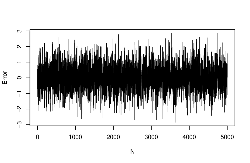
Secondly, we plot the histogram of the estimation error defined previously for a fixed value of $N=5000$ .

Random Time	Mean	Variance
Jittered Sampling	0.003081114	0.6664274
Renewal Sampling	-0.000968569	0.6666846

Table 4: Mean and variance of the estimation error

5.1 Conclusions

In relation to simulation results previously shown, we can state the following conclusions

•

It is quite easy to check, in Figure 1 for jittered sampling and Figure 2 for renewal sampling, that as the value of $N$ increases both type of random times are closer to their deterministic or equally spaced version.
•

When working with renewal observations, we consider an unbounded support so is quite likely that $\tau_{N}>1$ ; in order to avoid this, it was necessary to consider $\alpha\approx 1$ such that $\tau_{\alpha N}<1$ . The results given in Table 1 exhibits that for large values of $N$ and $\alpha$ close to $1$ , it is possible to ensure that $\tau_{\alpha N}<1$ .
•

It is possible to notice that, as the value of $N$ grows, the value of $Q_{N}$ is closer to $1/3$ .
•

In Figure 4 and in Table 2, it is possible to see the asymptotic normality of the renormalized sequence.
•

As we point out in theorem 1, the normal distribution with its corresponding parameters is shown in Figure 4 and Table 2, for both type of random times.
•

In both Figures 6, 7 and in Table 4, for both type of random times, the behavior of the error is as expected, i.e. is centered and with variance not depending on the value of $N$ and besides following a normal distribution.

6 Appendix

6.1 Proofs

Proof of Lemma 1: Let us separate the proof upon the two situations (2) and (4).

Jittered sampling case: In this case, as discussed in Section 2.2, we take $\alpha=1$ and $Y_{\tau_{N}}=0$ . Firstly, we compute the first moment of $A_{N}$ , i.e.

	$\displaystyle\mathbb{E}\left[A_{N}\right]$	$\displaystyle=\mathbb{E}\left[\mathbb{E}\left[A_{N}\mid\tau\right]\right]$
		$\displaystyle=\mathbb{E}\left[\mathbb{E}\left[\left.\dfrac{1}{N}\sum_{j=0}^{N-2}\left(\frac{j+1}{N}+\nu_{j}\right)\left(W_{\frac{j+1}{N}+\nu_{j+1}}-W_{\frac{j}{N}+\nu_{j}}\right)\right\|\nu\right]\right]$
		$\displaystyle=\mathbb{E}\left[\dfrac{1}{N}\sum_{j=0}^{N-2}\left(\frac{j+1}{N}+\nu_{j+1}\right)\mathbb{E}\left[W_{\frac{j+1}{N}+\nu_{j+1}}-W_{\frac{j}{N}+\nu_{j}}\mid\tau\right]\right]$
		$\displaystyle=0.$

The conditioning with respect to $\tau$ (above and throughout) means that we conditions with respect to the sigma-field generated by the random variables $\nu_{i,N},i=1,\ldots,N$ . The $L^{2}(\Omega)$ norm of $A_{N}$ can be calculated as follows

$\displaystyle\mathbb{E}\left[A_{N}^{2}\right]$	$\displaystyle=Var(A_{N})$
	$\displaystyle=\mathbb{E}\left[Var(A_{N}\mid\tau)\right]+Var(\mathbb{E}\left[A_{N}\mid\tau\right])=\mathbb{E}\left[Var(A_{N}\mid\tau)\right]$
	$\displaystyle=\mathbb{E}_{\nu}\left[\dfrac{1}{N^{2}}\sum_{j=0}^{N-2}\left(\frac{j+1}{N}+\nu_{j+1}\right)^{2}\left(\nu_{j+1}-\nu_{j}+\frac{1}{N}\right)\right]$
	$\displaystyle=\mathbb{E}\left[\dfrac{1}{N^{2}}\sum_{j=0}^{N-2}\left(\frac{(j+1)^{2}\nu_{j+1}}{N^{2}}+\frac{2(j+1)\nu_{j+1}^{2}}{N}+\nu_{j+1}^{3}-\frac{(j+1)^{2}\nu_{j}}{N^{2}}-\frac{2(j+1)\nu_{j}\nu_{j+1}}{N}\right.\right.$
	$\displaystyle-\left.\left.\nu_{j}\nu_{j+1}^{2}+\frac{(j+1)^{2}}{N^{3}}+\frac{2(j+1)\nu_{j+1}}{N^{2}}+\frac{\nu_{j+1}^{2}}{N}\right)\right]$
	$\displaystyle=:E_{N}^{(1)}+E_{N}^{(2)}+E_{N}^{(3)}-E_{N}^{(4)}-E_{N}^{(5)}-E_{N}^{(6)}+E_{N}^{(7)}+E_{N}^{(8)}+E_{N}^{(9)}.$	(14)

Notices that terms $E_{N}^{(1)},E_{N}^{(4)},E_{N}^{(5)},E_{N}^{(6)}$ and $E_{N}^{(8)}$ due to the assumption that $\mathbb{E}(\nu_{i,N})=0$ for every $i,N$ , $E_{N}^{(3)}$ is also equal to zero do the symmetry of the law of $\nu_{i,N}$ . Therefore

\displaystyle\mathbb{E}\left[A_{N}^{2}\right]

\displaystyle=

\displaystyle E_{N}^{(2)}+E_{N}^{(7)}+E_{N}^{(9)}.

(15)

We evaluate the three summands in the right-hand side above. By (3)

	$\displaystyle E_{N}^{(2)}$	$\displaystyle=\mathbb{E}\left[\dfrac{1}{N^{2}}\sum_{j=0}^{N-2}\dfrac{2\nu_{j+1}^{2}(j+1)}{N}\right]=\dfrac{2}{N^{3}}\sum_{j=0}^{N-2}(j+1)\mathbb{E}\left[\nu_{j+1}^{2}\right]$
		$\displaystyle=\dfrac{2c_{1}}{N^{5}}\left(\dfrac{N(N-1)}{2}\right)=\frac{c_{1}}{N^{3}}+o\left(\frac{1}{N^{3}}\right).$		(16)

	$\displaystyle E_{N}^{(7)}$	$\displaystyle=\mathbb{E}\left[\dfrac{1}{N^{2}}\sum_{j=0}^{N-2}\dfrac{(j+1)^{2}}{N^{3}}\right]=\dfrac{1}{N^{5}}\left(\dfrac{(N-1)(N)(2N-1)}{6}\right)$
		$\displaystyle=\frac{1}{3}\frac{1}{N^{2}}+o\left(\dfrac{1}{N^{2}}\right)$		(17)

and, again by (3), for $N\geq 2$ ,

\displaystyle E_{N}^{(9)}

\displaystyle=\mathbb{E}\left[\dfrac{1}{N^{2}}\sum_{j=0}^{N-2}\dfrac{\nu_{j+1}^{2}}{N}\right]=\dfrac{1}{N^{3}}\sum_{j=0}^{N-2}\mathbb{E}\left[\nu_{j+1}^{2}\right]=\dfrac{1}{N^{3}}\sum_{j=0}^{N-2}c_{1}\dfrac{1}{N^{2}}=c_{1}\dfrac{1}{(N-1)^{4}}.

(18)

From (15), (16), (17) and (18), we obtain the conclusion in JS case.

Renewal sampling case: Recall that in this case the number of observations is $N_{\alpha}=[\alpha N]$ with $\alpha<1$ close to $1$ . As before, by conditioning on $\tau$ ,

	$\displaystyle\mathbb{E}\left[A_{N}\right]$	$\displaystyle=\mathbb{E}\left[\mathbb{E}\left[A_{N}\|\tau\right]\right]=\left.\mathbb{E}\left[\mathbb{E}\left[\dfrac{1}{N}\sum_{j=0}^{N_{\alpha}-1}\tau_{j+1}\left(W_{\tau_{j+1}}-W_{\tau_{j}}\right)\right\|\tau\right]\right]$
		$\displaystyle=\mathbb{E}\left[\left.\dfrac{1}{N}\sum_{j=0}^{N_{\alpha}-1}\tau_{j+1}\mathbb{E}\left[W_{\tau_{j+1}}-W_{\tau_{j}}\right\|\tau\right]\right]=0,$

and, using that $A_{N}$ has, conditionally on $\tau$ , a Gaussian distribution, we obtain

$\displaystyle\mathbb{E}\left[A_{N}^{2}\right]$	$\displaystyle=Var(A_{N})=\mathbb{E}\left[Var(A_{N}\|\tau)\right]+Var(\mathbb{E}\left[A_{N}\|\tau\right])$
	$\displaystyle=\mathbb{E}\left[Var(A_{N}\|\tau)\right]=\mathbb{E}\left[Var\left(\dfrac{1}{N}\sum_{j=0}^{N_{\alpha}-1}\tau_{j+1}\left(W_{\tau_{j+1}}-W_{\tau_{j}}\right)\right)\right]$
	$\displaystyle=\mathbb{E}\left[\dfrac{1}{N^{2}}\sum_{j=0}^{N_{\alpha}-1}\tau_{j+1}^{2}\left(\tau_{j+1}-\tau_{j}\right)\right]=\mathbb{E}\left[\dfrac{1}{N^{2}}\sum_{j=0}^{N_{\alpha}-1}\tau_{j+1}^{3}-\dfrac{1}{N^{2}}\sum_{j=0}^{N_{\alpha}-1}\tau_{j+1}^{2}\tau_{j}\right]$
	$\displaystyle=\dfrac{1}{N^{2}}\sum_{j=0}^{N_{\alpha}-1}\mathbb{E}\left[\tau_{j+1}^{3}\right]-\dfrac{1}{N^{2}}\sum_{j=0}^{N_{\alpha}-1}\mathbb{E}\left[\tau_{j+1}^{2}\tau_{j}\right]=:E_{N}^{(1)}-E_{N}^{(2)}.$	(19)

For the first term of (19), we have

$\displaystyle E_{N}^{(1)}$	$\displaystyle=\dfrac{1}{N^{2}}\sum_{j=0}^{N_{\alpha}-1}\mathbb{E}\left[\tau_{j+1}^{3}\right]=\dfrac{1}{N^{2}}\sum_{j=0}^{N_{\alpha}-1}\int_{0}^{\infty}x^{3}\dfrac{N^{j+1}}{\Gamma(j+1)}x^{j}e^{-Nx}dx$
	$\displaystyle=\dfrac{1}{N^{2}}\sum_{j=0}^{N-1}\dfrac{N^{j+1}}{N^{j+4}}\dfrac{\Gamma(j+4)}{\Gamma(j+1)}=\dfrac{1}{N^{2}}\sum_{j=0}^{N_{\alpha}-1}\dfrac{(j+3)(j+2)(j+1)\Gamma(j+1)}{N^{3}\Gamma(j+1)}$
	$\displaystyle=\dfrac{1}{N^{5}}\sum_{j=0}^{N_{\alpha}-1}(j^{3}+6j^{2}+11j+6)$
	$\displaystyle=\dfrac{1}{N^{5}}\left(\dfrac{(N_{\alpha}-1)(N_{\alpha})}{2}\right)^{2}+\dfrac{(N_{\alpha}-1)(N_{\alpha})(2(N_{\alpha}-1)+1)}{N^{5}}+\dfrac{11}{2}\dfrac{(N_{\alpha}-1)(N_{\alpha})}{N^{5}}+\dfrac{6N_{\alpha}}{N^{5}}$
	$\displaystyle\sim\frac{\alpha^{4}}{4N}+\frac{3\alpha^{3}}{N^{2}}+o\left(\frac{1}{N^{2}}\right).$	(20)

For the second term of (19), we consider the joint density computed by Araya et al. 2019 (see Table (5))

$\displaystyle E_{N}^{(2)}$	$\displaystyle=\dfrac{1}{N^{2}}\sum_{j=0}^{N_{\alpha}-1}\mathbb{E}\left[\tau_{j+1}^{2}\tau_{j}\right]=\dfrac{1}{N^{2}}\sum_{j=0}^{N_{\alpha}-1}\int_{0}^{\infty}\int_{0}^{\tau_{j+1}}\tau_{j}\tau_{j+1}^{2}\dfrac{N^{j+1}}{\Gamma(j)}\tau_{j}^{j-1}e^{-N\tau_{j+1}}d\tau_{j}d\tau_{j+1}$
	$\displaystyle=\dfrac{1}{N^{2}}\sum_{j=0}^{N_{\alpha}-1}\dfrac{N^{j+1}}{\Gamma(j)}\int_{0}^{\infty}\tau_{j+1}^{2}e^{-N\tau_{j+1}}\int_{0}^{\tau_{j+1}}\tau_{j}^{j}d\tau_{j}d\tau_{j+1}$
	$\displaystyle=\dfrac{1}{N^{2}}\sum_{j=0}^{N_{\alpha}-1}\dfrac{N^{j+1}}{(j+1)\Gamma(j)}\int_{0}^{\infty}\tau_{j+1}^{j+3}e^{-N\tau_{j+1}}d\tau_{j+1}=\dfrac{1}{N^{2}}\sum_{j=0}^{N_{\alpha}-1}\dfrac{N^{j+1}}{(j+1)\Gamma(j)}\dfrac{\Gamma(j+4)}{N^{j+4}}$
	$\displaystyle=\dfrac{1}{N^{5}}\sum_{j=0}^{N_{\alpha}-1}\dfrac{(j+3)(j+2)(j+1)j\Gamma(j)}{(j+1)\Gamma(j)}=\dfrac{1}{N^{5}}\sum_{j=0}^{N_{\alpha}-1}(j^{3}+5j^{2}+6j)$
	$\displaystyle=\dfrac{1}{N^{5}}\left(\dfrac{(N_{\alpha}-1)(N_{\alpha})}{2}\right)^{2}+\dfrac{5}{N^{5}}\left(\dfrac{(N_{\alpha}-1)(N_{\alpha})(2(N_{\alpha}-1)+1)}{6}\right)+\dfrac{6}{N^{5}}\left(\dfrac{(N_{\alpha}-1)(N_{\alpha})}{2}\right)$
	$\displaystyle\sim\dfrac{\alpha^{4}}{4N}+\dfrac{7\alpha^{3}}{6N^{2}}+o\left(\frac{1}{N^{2}}\right).$	(21)

Replacing (20) and (21) in (19)

\displaystyle\mathbb{E}\left[A_{N}^{2}\right]

\displaystyle\sim\dfrac{\alpha^{3}}{3N^{2}}+o\left(\frac{1}{N^{2}}\right).

(22)

Proof of Proposition 2: Again, we separately discuss the two cases of random sampling.

Jittered sampling case: Recall that in this case $\alpha=1$ . First, we compute the first moment of (9), i.e

	$\displaystyle\mathbb{E}\left[Q_{N}\right]$	$\displaystyle=\mathbb{E}\left[\sum_{j=0}^{N-1}\left(\frac{j+1}{N}+\frac{X_{j+1}}{N}\right)^{2}\left(\frac{X_{j+1}}{N}-\frac{X_{j}}{N}+\frac{1}{N}\right)\right]$
		$\displaystyle=\dfrac{1}{N^{3}}\sum_{j=0}^{N-1}\mathbb{E}\left[(j+1)^{2}X_{j+1}-(j+1)^{2}X_{j}+(j+1)^{2}+2(j+1)X_{j+1}^{2}-2(j+1)X_{j}X_{j+1}\right.$
		$\displaystyle\left.+2(j+1)X_{j+1}+X_{j+1}^{3}-X_{j}X_{j+1}^{2}+X_{j+1}^{2}\right]$
		$\displaystyle=\dfrac{1}{N^{3}}\sum_{j=0}^{N-1}\left[Q_{N}^{(1)}-Q_{N}^{(2)}+Q_{N}^{(3)}+Q_{N}^{(4)}-Q_{N}^{(5)}+Q_{N}^{(6)}+Q_{N}^{(7)}-Q_{N}^{(8)}+Q_{N}^{(9)}\right].$

From (10) and the hypothesis (3) on $\tau$ , we have

\mathbb{E}(X_{j})=0\mbox{ and }\mathbb{E}(X_{j}^{2})=c_{1}.

Thus $Q_{N}^{(1)}$ , $Q_{N}^{(2)}$ , $Q_{N}^{(5)}$ , $Q_{N}^{(6)}$ , $Q_{N}^{(7)}$ and $Q_{N}^{(8)}$ are equal to zero, while the remaining terms can be computed as follows

	$\displaystyle Q_{N}^{(3)}$	$\displaystyle=\mathbb{E}\left[\dfrac{1}{N^{3}}\sum_{j=0}^{N-1}(j+1)^{2}\right]=\dfrac{N(N+1)(2N+1)}{6}$
		$\displaystyle=\dfrac{2N^{3}+3N^{2}+N}{6}\xrightarrow[N\to\infty]{}\dfrac{1}{3}$		(23)

	$\displaystyle Q_{N}^{(4)}$	$\displaystyle=\mathbb{E}\left[\dfrac{1}{N^{3}}\sum_{j=0}^{N-1}2(j+1)X_{j+1}^{2}\right]=\dfrac{2}{N^{3}}\sum_{j=0}^{N-1}(j+1)Var\left(X_{j+1}^{2}\right)$
		$\displaystyle=\dfrac{2}{N^{3}}\sum_{j=0}^{N-1}(j+1)\dfrac{1}{12}=\dfrac{1}{6N^{3}}\left(\dfrac{N(N+1)}{2}\right)\xrightarrow[N\to\infty]{}0$		(24)

and

	$\displaystyle Q_{N}^{(9)}$	$\displaystyle=\mathbb{E}\left[\dfrac{1}{N^{3}}\sum_{j=0}^{N-1}X_{j+1}^{2}\right]=\dfrac{1}{N^{3}}\sum_{j=0}^{N-1}Var\left(X_{j+1}\right)$
		$\displaystyle=\dfrac{1}{N^{3}}\sum_{j=0}^{N-1}c_{1}\xrightarrow[N\to\infty]{}0$		(25)

Taking into account (23), (24) and (25) we conclude

\lim_{N\to\infty}\mathbb{E}\left[Q_{N}\right]\xrightarrow[N\to\infty]{}\dfrac{1}{3}.

(26)

Secondly, we study the second moment of (9), i.e.

	$\displaystyle\mathbb{E}\left[Q_{N}^{2}\right]$	$\displaystyle=\dfrac{1}{N^{6}}\sum_{j=0}^{N-1}\mathbb{E}\left[(j+1+X_{j+1})^{4}(X_{j+1}-X_{j}+1)^{2}\right]$
		$\displaystyle+\dfrac{1}{N^{6}}\sum_{0\leq j\neq k\leq N-1}\mathbb{E}\left[(j+1+X_{j+1})^{2}(k+1+X_{k+1})^{2}(X_{j+1}-X_{j}+1)(X_{k+1}-X_{k}+1)\right]$
		$\displaystyle:=Q_{N}^{(I)}+Q_{N}^{(II)}.$

Some of the summands that compose $Q_{N}^{(I)}$ are zero (those involving odd order moments of $X_{j}$ or $X_{j+1}$ , which vanish) and the other summands of $Q_{N}^{(I)}$ converge to zero. For example

	$\displaystyle\mathbb{E}\left[\dfrac{1}{N^{6}}\sum_{j=0}^{N-1}(j+1)^{4}X_{j+1}^{2}\right]$	$\displaystyle=\dfrac{1}{N^{6}}\sum_{j=0}^{N-1}(j+1)^{4}Var(X_{j+1})$
		$\displaystyle=\dfrac{c_{1}}{N^{6}}\left(\dfrac{6N^{5}+15N^{4}+10N^{3}-N}{30}\right)\xrightarrow[N\to\infty]{}0$

\displaystyle\mathbb{E}\left[\dfrac{1}{N^{6}}\sum_{j=0}^{N-1}2(j+1)^{4}X_{j}X_{j+1}\right]

\displaystyle=\dfrac{2}{N^{6}}\sum_{j=0}^{N-1}(j+1)\mathbb{E}\left[X_{j}X_{j+1}\right]=0

while the remaining terms can be computed in the same way as the last two.

The summand $Q_{N}^{(II)}$ give the limit of $Q_{N}$ . Actually, the only non-vanishing term in $Q_{N}^{(II)}$ is the one not depending on $X_{j}$ , i.e.

\displaystyle\mathbb{E}\left[\dfrac{1}{N^{6}}\sum_{0\leq j\neq k\leq N-1}(j+1)^{2}(k+1)^{2}\right]

\displaystyle=\dfrac{1}{N^{6}}\sum_{0\leq j\neq k\leq N-1}(j+1)^{2}(k+1)^{2}.

To compute this term, we use the following identity

\displaystyle\sum_{1\leq i\neq j\leq N}a_{i}a_{j}

\displaystyle=\left(\sum_{i=1}^{N}a_{i}\right)^{2}-\sum_{i=1}^{N}a_{i}^{2}

(27)

Therefore,

		$\displaystyle\dfrac{1}{N^{6}}\sum_{0\leq j\neq k\leq N-1}(j+1)^{2}(k+1)^{2}=\dfrac{1}{N^{6}}\left[\left(\sum_{j=0}^{N-1}(j+1)^{2}\right)^{2}\sum_{j=0}^{N-1}(j+1)^{4}\right]$
		$\displaystyle=\dfrac{1}{N^{6}}\left[\left(\dfrac{N(N+1)(2N+1)}{6}\right)^{2}-\left(\dfrac{6N^{5}+15N^{4}+10N^{3}-N}{30}\right)\right]$
		$\displaystyle=\dfrac{1}{N^{6}}\left[\dfrac{(2N^{3}+3N^{2}+N)^{2}}{36}-\dfrac{6N^{5}-15N^{4}-10N^{3}+N}{30}\right]\xrightarrow[N\to\infty]{}\dfrac{1}{9}.$		(28)

Taking into account (26) and (28), we obtain the conclusion.

Renewal sampling case: As before, we start by computing the expectation of $Q_{N}$ . We have

	$\displaystyle\mathbb{E}\left[Q_{N}\right]$	$\displaystyle=\mathbb{E}\left[\sum_{j=0}^{N_{\alpha}-1}\tau_{j+1}^{2}\left(\tau_{j+1}-\tau_{j}\right)\right]$
		$\displaystyle=\mathbb{E}\left[\sum_{j=0}^{N_{\alpha}-1}\tau_{j+1}^{3}\right]-\mathbb{E}\left[\sum_{j=0}^{N_{\alpha}-1}\tau_{j+1}^{2}\tau_{j}\right]=Q_{N}^{(1)}-Q_{N}^{(2)}$		(29)

with

$\displaystyle Q_{N}^{(1)}$	$\displaystyle=\mathbb{E}\left[\sum_{j=0}^{N-1}\tau_{j+1}^{3}\right]=\sum_{j=0}^{N_{\alpha}-1}\int_{0}^{\infty}\tau_{j+1}^{3}\dfrac{N^{j+1}}{\Gamma(j+1)}\tau_{j+1}^{j}e^{-N\tau_{j+1}}d\tau_{j+1}$
	$\displaystyle=\sum_{j=0}^{N_{\alpha}-1}\dfrac{N^{j+1}}{\Gamma(j+1)}\dfrac{\Gamma(j+4)}{N^{j+4}}=\dfrac{1}{N^{3}}\sum_{j=0}^{N_{\alpha}-1}(j+3)(j+2)(j+1)$
	$\displaystyle=\dfrac{1}{N^{3}}\sum_{j=0}^{N_{\alpha}-1}[j^{3}+6j^{2}+11j+6]$	(30)

and

$\displaystyle Q_{N}^{(2)}$	$\displaystyle=\mathbb{E}\left[\sum_{j=0}^{N_{\alpha}-1}\tau_{j+1}^{2}\tau_{j}\right]=\sum_{j=0}^{N_{\alpha}-1}\int_{0}^{\infty}\int_{0}^{\tau_{j+1}}\tau_{j+1}^{2}\tau_{j}\dfrac{N^{j+1}}{\Gamma(j)}\tau_{j}^{j-1}e^{-N\tau_{j+1}}d\tau_{j}d\tau_{j+1}$
	$\displaystyle=\sum_{j=0}^{N_{\alpha}-1}\dfrac{N^{j+1}}{\Gamma(j)}\int_{0}^{\infty}\tau_{j+1}^{2}e^{-N\tau_{j+1}}\int_{0}^{\tau_{j+1}}\tau_{j}^{j}d\tau_{j}d\tau_{j+1}=\sum_{j=0}^{N_{\alpha}-1}\dfrac{N^{j+1}}{\Gamma(j)(j+1)}\int_{0}^{\infty}\tau_{j+1}^{j+4-1}e^{-N\tau_{j+1}}d\tau_{j+1}$
	$\displaystyle=\sum_{j=0}^{N_{\alpha}-1}\dfrac{N^{j+1}}{N^{j+4}}\dfrac{\Gamma(j+4)}{\Gamma(j)(j+1)}=\dfrac{1}{N^{3}}\sum_{j=0}^{N_{\alpha}-1}(j+3)(j+2)j=\dfrac{1}{N^{3}}\sum_{j=0}^{N_{\alpha}-1}[j^{3}-5j^{2}+6j].$	(31)

Replacing (30) and (31) in (29), it results

\displaystyle\mathbb{E}\left[Q_{N}\right]

\displaystyle=\dfrac{1}{N^{3}}\sum_{j=0}^{N_{\alpha}-1}[j^{2}-5j+6]=\dfrac{1}{N^{3}}\left[\dfrac{2N_{\alpha}^{3}-18N_{\alpha}^{2}+52N_{\alpha}}{6}\right]\xrightarrow[N\to\infty]{}\dfrac{\alpha^{3}}{3}

For the second moment of $Q_{N}$ we have

$\displaystyle\mathbb{E}\left[Q_{N}^{2}\right]$	$\displaystyle=\mathbb{E}\left[\left(\sum_{j=0}^{N_{\alpha}-1}\tau_{j+1}^{2}\left(\tau_{j+1}-\tau_{j}\right)\right)^{2}\right]$
	$\displaystyle=\mathbb{E}\left[\sum_{j=0}^{N_{\alpha}-1}\tau_{j+1}^{4}\left(\tau_{j+1}-\tau_{j}\right)^{2}\right]+2\mathbb{E}\left[\sum_{j<k}^{N_{\alpha}-1}\tau_{j+1}^{2}\tau_{k+1}^{2}\left(\tau_{j+1}-\tau_{j}\right)\left(\tau_{k+1}-\tau_{k}\right)\right]$
	$\displaystyle=\mathbb{E}\left[\sum_{j=0}^{N_{\alpha}-1}\tau_{j+1}^{6}-2\sum_{j=0}^{N_{\alpha}-1}\tau_{j+1}^{5}\tau_{j}+\sum_{j=0}^{N_{\alpha}-1}\tau_{j+1}^{4}\tau_{j}^{2}\right]$
	$\displaystyle+2\mathbb{E}\left[\sum_{j<k}^{N_{\alpha}-1}\tau_{j+1}^{3}\tau_{k+1}^{3}-\sum_{j<k}^{N_{\alpha}-1}\tau_{j+1}^{3}\tau_{k}\tau_{k+1}^{2}-\sum_{j<k}^{N_{\alpha}-1}\tau_{j+1}^{2}\tau_{j}\tau_{k+1}^{3}+\sum_{j<k}^{N_{\alpha}-1}\tau_{j}\tau_{j+1}^{2}\tau_{k}\tau_{k+1}^{2}\right]$
	$\displaystyle:=Q_{N}^{(I)}-Q_{N}^{(II)}+Q_{N}^{(III)}+Q_{N}^{(IV)}-Q_{N}^{(V)}-Q_{N}^{(VI)}+Q_{N}^{(VII)}$	(32)

and the above terms can be calculated by using the joint densities from Table 5. We calculate first the sum $Q_{N}^{(I)}-Q_{N}^{(II)}+Q_{N}^{(III)}$ . First

$\displaystyle Q_{N}^{(I)}$	$\displaystyle=\mathbb{E}\left[\sum_{j=0}^{N_{\alpha}-1}\tau_{j+1}^{6}\right]=\sum_{j=0}^{N_{\alpha}-1}\int_{0}^{\infty}\tau_{j+1}^{6}\dfrac{N^{j+1}}{\Gamma(j+1)}\tau_{j+1}^{j}e^{-N\tau_{j+1}}d\tau_{j+1}$
	$\displaystyle=\sum_{j=0}^{N_{\alpha}-1}\dfrac{N^{j+1}}{\Gamma(j+1)}\int_{0}^{\infty}\tau_{j+1}^{j+7-1}e^{-N\tau_{j+1}}d\tau_{j+1}=\sum_{j=0}^{N_{\alpha}-1}\dfrac{N^{j+1}}{N^{j+7}}\dfrac{\Gamma(j+7)}{\Gamma(j+1)}$
	$\displaystyle=\dfrac{1}{N^{6}}\sum_{j=0}^{N_{\alpha}-1}(j+6)(j+5)(j+4)(j+3)(j+2)(j+1)$
	$\displaystyle=\dfrac{1}{N^{6}}\sum_{j=0}^{N_{\alpha}-1}[j^{6}+21j^{5}+175j^{4}+735j^{3}+1624j^{2}+1764j+720].$	(33)

For $Q_{N}^{(II)},Q_{N}^{(III)}$ we use the joint density of the random vector $(\tau_{j},\tau_{k})$

$\displaystyle Q_{N}^{(II)}$	$\displaystyle=2\mathbb{E}\left[\sum_{j=0}^{N_{\alpha}-1}\tau_{j+1}^{5}\tau_{j}\right]=2\sum_{j=0}^{N_{\alpha}-1}\int_{0}^{\infty}\int_{0}^{\tau_{j+1}}\tau_{j+1}^{5}\tau_{j}\dfrac{N^{j+1}}{\Gamma(j)}\tau_{j}^{j-1}e^{-N\tau_{j+1}}d\tau_{j}d\tau_{j+1}$
	$\displaystyle=2\sum_{j=0}^{N_{\alpha}-1}\dfrac{N^{j+1}}{\Gamma(j)}\int_{0}^{\infty}\tau_{j+1}^{5}e^{-N\tau_{j+1}}\int_{0}^{\tau_{j+1}}\tau_{j}^{j}d\tau_{j}d\tau_{j+1}$
	$\displaystyle=2\sum_{j=0}^{N_{\alpha}-1}\dfrac{N^{j+1}}{\Gamma(j)(j+1)}\int_{0}^{\infty}\tau_{j+1}^{j+7-1}e^{-N\tau_{j+1}}d\tau_{j+1}$
	$\displaystyle=2\sum_{j=0}^{N_{\alpha}-1}\dfrac{N^{j+1}}{N^{j+7}}\dfrac{\Gamma(j+7)}{\Gamma(j)(j+1)}=\dfrac{2}{N^{6}}\sum_{j=0}^{N_{\alpha}-1}(j+6)(j+5)(j+4)(j+3)(j+2)j$
	$\displaystyle=\dfrac{1}{N^{6}}\sum_{j=0}^{N_{\alpha}-1}[2j^{6}+40j^{5}+310j^{4}+1160j^{3}+2088j^{2}+1440j]$	(34)

and

$\displaystyle Q_{N}^{(III)}$	$\displaystyle=\mathbb{E}\left[\sum_{j=0}^{N_{\alpha}-1}\tau_{j+1}^{4}\tau_{j}^{2}\right]=\sum_{j=0}^{N_{\alpha}-1}\int_{0}^{\infty}\int_{0}^{\tau_{j+1}}\tau_{j+1}^{4}\tau_{j}^{2}\dfrac{N^{j+1}}{\Gamma(j)}\tau_{j}^{j-1}e^{-N\tau_{j+1}}d\tau_{j}d\tau_{j+1}$
	$\displaystyle=\sum_{j=0}^{N_{\alpha}-1}\dfrac{N^{j+1}}{\Gamma(j)}\int_{0}^{\infty}\tau_{j+1}^{4}e^{-N\tau_{j+1}}\int_{0}^{\tau_{j+1}}\tau_{j}^{j+1}d\tau_{j}d\tau_{j+1}$
	$\displaystyle=\sum_{j=0}^{N_{\alpha}-1}\dfrac{N^{j+1}}{\Gamma(j)(j+2)}\int_{0}^{\infty}\tau_{j+1}^{j+7-1}e^{-N\tau_{j+1}}d\tau_{j+1}$
	$\displaystyle=\sum_{j=0}^{N_{\alpha}-1}\dfrac{N^{j+1}}{N^{j+7}}\dfrac{\Gamma(j+7)}{\Gamma(j)(j+2)}=\dfrac{1}{N^{6}}\sum_{j=0}^{N_{\alpha}-1}(j+6)(j+5)(j+4)(j+3)(j+1)j$
	$\displaystyle=\dfrac{1}{N^{6}}\sum_{j=0}^{N_{\alpha}-1}[j^{6}+19j^{5}+137j^{4}+461j^{3}+702j^{2}+360j].$	(35)

By putting together (33), (34) and (35),

\displaystyle Q_{N}^{(I)}-Q_{N}^{(II)}+Q_{N}^{(III)}=\dfrac{1}{N^{6}}\sum_{j=0}^{N_{\alpha}-1}[j^{4}+18j^{3}+119j^{2}+342j+360]\xrightarrow[N\to\infty]{}0,

(36)

For terms $Q_{N}^{(IV)},Q_{N}^{(V)},Q_{N}^{(VI)}$ and $Q_{N}^{(VII)}$ it is necessary to consider the following joint densities $f_{\tau_{j+1},\tau_{k+1}}$ , $f_{\tau_{j},\tau_{k},\tau_{l}}$ and $f_{\tau_{j},\tau_{k},\tau_{l},\tau_{m}}$ with all the different indices. We also use the identity

\int_{0}^{b}x^{a}(b-x)^{c}dx=\dfrac{\Gamma(a+1)\Gamma(c+1)}{\Gamma(a+c+2)}b^{a+c+1}.

(37)

We have the following calculations

$\displaystyle Q_{N}^{(IV)}$	$\displaystyle=\mathbb{E}\left[\sum_{j<k}^{N_{\alpha}-1}\tau_{j+1}^{3}\tau_{k+1}^{3}\right]$
	$\displaystyle=\sum_{j<k}^{N_{\alpha}-1}\int_{0}^{\infty}\int_{0}^{\tau_{k+1}}\tau_{j+1}^{3}\tau_{k+1}^{3}\dfrac{N^{k+1}}{\Gamma(j+1)\Gamma(k-j)}\tau_{j+1}^{j}(\tau_{k+1}-\tau_{j+1})^{k-j-1}e^{-N\tau_{k+1}}d\tau_{j+1}d\tau_{k+1}$
	$\displaystyle=\sum_{j<k}^{N_{\alpha}-1}\dfrac{N^{k+1}}{\Gamma(j+1)\Gamma(k-j)}\int_{0}^{\infty}\tau_{k+1}^{3}e^{-N\tau_{k+1}}\int_{0}^{\tau_{k+1}}\tau_{j+1}^{j+3}(\tau_{k+1}-\tau_{j+1})^{k-j-1}d\tau_{j+1}d\tau_{k+1}$
	$\displaystyle=\sum_{j<k}^{N_{\alpha}-1}\dfrac{N^{k+1}}{\Gamma(j+1)\Gamma(k-j)}\dfrac{\Gamma(j+4)\Gamma(k-j)}{\Gamma(k+4)}\int_{0}^{\infty}\tau_{k+1}^{k+7-1}e^{-N\tau_{k+1}}d\tau_{k+1}$
	$\displaystyle=\sum_{j<k}^{N_{\alpha}-1}\dfrac{N^{k+1}}{N^{k+7}}\dfrac{\Gamma(j+4)\Gamma(k+7)}{\Gamma(j+1)\Gamma(k+4)}=\dfrac{1}{N^{6}}\sum_{j<k}^{N_{\alpha}-1}(j+3)(j+2)(j+1)(k+6)(k+5)(k+4),$	(38)

and, via (37)

$\displaystyle Q_{N}^{(V)}$	$\displaystyle=\mathbb{E}\left[\sum_{j<k}^{N_{\alpha}-1}\tau_{j+1}^{3}\tau_{k}\tau_{k+1}^{2}\right]$
	$\displaystyle=\sum_{j<k}^{N_{\alpha}-1}\int_{0}^{\infty}\int_{0}^{\tau_{k+1}}\int_{0}^{\tau_{k}}\tau_{j+1}^{3}\tau_{k}\tau_{k+1}^{2}\dfrac{N^{k+1}}{\Gamma(j+1)\Gamma(k-j-1)}\tau_{j+1}^{j}(\tau_{k}-\tau_{j+1})^{k-j-2}e^{-N\tau_{k+1}}d\tau_{j+1}d\tau_{k}d\tau_{k+1}$
	$\displaystyle=\sum_{j<k}^{N_{\alpha}-1}\dfrac{N^{k+1}}{\Gamma(j+1)\Gamma(k-j-1)}\int_{0}^{\infty}\tau_{k+1}^{2}e^{-N\tau_{k+1}}\int_{0}^{\tau_{k+1}}\tau_{k}\int_{0}^{\tau_{k}}\tau_{j+1}^{j+3}(\tau_{k}-\tau_{j+1})^{k-j-2}d\tau_{j+1}d\tau_{k}d\tau_{k+1}$
	$\displaystyle=\sum_{j<k}^{N_{\alpha}-1}\dfrac{N^{k+1}}{\Gamma(j+1)\Gamma(k-j-1)}\dfrac{\Gamma(j+4)\Gamma(k-j-1)}{\Gamma(k+3)}\int_{0}^{\infty}\tau_{k+1}^{2}e^{-N\tau_{k+1}}\int_{0}^{\tau_{k+1}}\tau_{k}^{k+3}d\tau_{k}d\tau_{k+1}$
	$\displaystyle=\sum_{j<k}^{N_{\alpha}-1}\dfrac{N^{k+1}\Gamma(j+4}{\Gamma(j+1)\Gamma(k+3)(k+4)}\int_{0}^{\infty}\tau_{k+1}^{k+7-1}e^{-N\tau_{k+1}}d\tau_{k+1}$
	$\displaystyle=\sum_{j<k}^{N_{\alpha}-1}\dfrac{N^{k+1}}{N^{k+7}}\dfrac{\Gamma(j+4)\Gamma(k+7)}{\Gamma(j+1)\Gamma(k+3)(k+4)}=\dfrac{1}{N^{6}}\sum_{j<k}^{N_{\alpha}-1}(j+3)(j+2)(j+1)(k+6)(k+5)(k+3)$	(39)

and

$\displaystyle Q_{N}^{(VI)}$	$\displaystyle=\mathbb{E}\left[\sum_{j<k}^{N_{\alpha}-1}\tau_{j+1}^{2}\tau_{j}\tau_{k+1}^{3}\right]$
	$\displaystyle=\sum_{j<k}^{N_{\alpha}-1}\int_{0}^{\infty}\int_{0}^{\tau_{k+1}}\int_{0}^{\tau_{j+1}}\tau_{j+1}^{2}\tau_{j}\tau_{k+1}^{3}\dfrac{N^{k+1}}{\Gamma(j)\Gamma(k-j)}\tau_{j}^{j-1}(\tau_{k+1}-\tau_{j+1})^{k-j-1}e^{-N\tau_{k+1}}d\tau_{j}d\tau_{j+1}d\tau_{k+1}$
	$\displaystyle=\sum_{j<k}^{N_{\alpha}-1}\dfrac{N^{k+1}}{\Gamma(j)\Gamma(k-j)}\int_{0}^{\infty}\tau_{k+1}^{3}e^{-N\tau_{k+1}}\int_{0}^{\tau_{k+1}}\tau_{j+1}^{2}(\tau_{k+1}-\tau_{j+1})^{k-j-1}\int_{0}^{\tau_{j+1}}\tau_{j}^{j}d\tau_{j}d\tau_{j+1}d\tau_{k+1}$
	$\displaystyle=\sum_{j<k}^{N_{\alpha}-1}\dfrac{N^{k+1}}{\Gamma(j)\Gamma(k-j)(j+1)}\int_{0}^{\infty}\tau_{k+1}^{3}e^{-N\tau_{k+1}}\int_{0}^{\tau_{k+1}}\tau_{j+1}^{j+3}(\tau_{k+1}-\tau_{j+1})^{k-j-1}d\tau_{j+1}d\tau_{k+1}$
	$\displaystyle=\sum_{j<k}^{N_{\alpha}-1}\dfrac{N^{k+1}}{\Gamma(j)\Gamma(k-j)(j+1)}\dfrac{\Gamma(j+4)\Gamma(k-j)}{\Gamma(k+4)}\int_{0}^{\infty}\tau_{k+1}^{k+7-1}e^{-N\tau_{k+1}}d\tau_{k+1}$
	$\displaystyle=\sum_{j<k}^{N_{\alpha}-1}\dfrac{N^{k+1}}{N^{k+7}}\dfrac{\Gamma(j+4)\Gamma(k+7)}{\Gamma(j)(j+1)\Gamma(k+4)}=\dfrac{1}{N^{6}}\sum_{j<k}^{N_{\alpha}-1}(j+3)(j+2)j(k+6)(k+5)(k+4)$	(40)

and finally

$\displaystyle Q_{N}^{(VII)}$	$\displaystyle=\mathbb{E}\left[\sum_{j<k}^{N_{\alpha}-1}\tau_{j}\tau_{j+1}^{2}\tau_{k}\tau_{k+1}^{2}\right]$
	$\displaystyle=\sum_{j<k}^{N_{\alpha}-1}\int_{0}^{\infty}\int_{0}^{\tau_{k+1}}\int_{0}^{\tau_{k}}\int_{0}^{\tau_{j+1}}\tau_{j}\tau_{j+1}^{2}\tau_{k}\tau_{k+1}^{2}\dfrac{N^{k+1}}{\Gamma(j)\Gamma(k-j-1)}\tau_{j}^{j-1}(\tau_{k}-\tau_{j+1})^{k-j-2}e^{-N\tau_{k+1}}d\tau_{j}d\tau_{j+1}d\tau_{k}d\tau_{k+1}$
	$\displaystyle=\sum_{j<k}^{N_{\alpha}-1}\dfrac{N^{k+1}}{\Gamma(j)\Gamma(k-j-1)}\int_{0}^{\infty}\tau_{k+1}^{2}e^{-N\tau_{k+1}}\int_{0}^{\tau_{k+1}}\tau_{k}\int_{0}^{\tau_{k}}\tau_{j+1}^{2}(\tau_{k}-\tau_{j+1})^{k-j-2}\int_{0}^{\tau_{j+1}}\tau_{j}^{j}d\tau_{j}d\tau_{j+1}d\tau_{k}d\tau_{k+1}$
	$\displaystyle=\sum_{j<k}^{N_{\alpha}-1}\dfrac{N^{k+1}}{\Gamma(j)\Gamma(k-j-1)(j+1)}\int_{0}^{\infty}\tau_{k+1}^{2}e^{-N\tau_{k+1}}\int_{0}^{\tau_{k+1}}\tau_{k}\int_{0}^{\tau_{k}}\tau_{j+1}^{j+3}(\tau_{k}-\tau_{j+1})^{k-j-2}d\tau_{j+1}d\tau_{k}d\tau_{k+1}$
	$\displaystyle=\sum_{j<k}^{N_{\alpha}-1}\dfrac{N^{k+1}}{\Gamma(j)\Gamma(k-j-1)(j+1)}\dfrac{\Gamma(j+4)\Gamma(k-j-1)}{\Gamma(k+3}\int_{0}^{\infty}\tau_{k+1}^{2}e^{-N\tau_{k+1}}\int_{0}^{\tau_{k+1}}\tau_{k+3}d\tau_{k}d\tau_{k+1}$
	$\displaystyle=\sum_{j<k}^{N_{\alpha}-1}\dfrac{N^{k+1}\Gamma(j+4)}{\Gamma(j)(j+1)\Gamma(k+3)(k+4)}\int_{0}^{\infty}\tau_{k+1}^{k-7-1}e^{-N\tau_{k+1}}d\tau_{k+1}$
	$\displaystyle=\sum_{j<k}^{N_{\alpha}-1}\dfrac{N^{k+1}}{N^{k+7}}\dfrac{\Gamma(j+4)\Gamma(k+7)}{\Gamma(j)(j+1)\Gamma(k+3)(k+4)}=\dfrac{1}{N^{6}}\sum_{j<k}^{N_{\alpha}-1}(j+3)(j+2)j(k+6)(k+5)(k+3).$	(41)

Taking into account the results from (38), (39), (40) and (41), we get

	$\displaystyle Q_{N}^{(IV)}-Q_{N}^{(V)}-Q_{N}^{(VI)}+Q_{N}^{(VII)}$	$\displaystyle=\dfrac{2}{N^{6}}\sum_{j<k}^{N-1}\left[(j+3)(j+2)(j+1)(k+6)(k+5)(k+4)\right.$
		$\displaystyle-(j+3)(j+2)(j+1)(k+6)(k+5)(k+3)$
		$\displaystyle-(j+3)(j+2)j(k+6)(k+5)(k+4)$
		$\displaystyle+\left.(j+3)(j+2)j(k+6)(k+5)(k+3)\right]$
		$\displaystyle=\dfrac{2}{N^{6}}\sum_{j<k}^{N-1}\left[(j+3)(j+2)(j+1)(k+6)(k+5)\left[(k+4)-(k+3)\right]\right.$
		$\displaystyle+\left.(j+3)(j+2)j(k+6)(k+5)\left[(k+3)-(k+4)\right]\right]$
		$\displaystyle=\dfrac{2}{N^{6}}\sum_{j<k}^{N-1}\left[(j+3)(j+2)(k+6)(k+5)\left[(j+1)-j\right]\right]$
		$\displaystyle=\dfrac{2}{N^{6}}\sum_{j<k}^{N-1}\left[(j+3)(j+2)(k+6)(k+5\right]$

and this can be written as

$\displaystyle Q_{N}^{(IV)}-Q_{N}^{(V)}-Q_{N}^{(VI)}+Q_{N}^{(VII)}$	$\displaystyle=\dfrac{2}{N^{6}}\sum_{k=1}^{N_{\alpha}-1}(k+6)(k+5)\sum_{j=0}^{k-1}(j+3)(j+2)$
	$\displaystyle\sim\dfrac{2}{N^{6}}\sum_{k=1}^{N_{\alpha}-1}(k+6)(k+5)k^{3}+o\left(\frac{1}{N}\right)$
	$\displaystyle\sim\frac{2}{18}\frac{(N_{\alpha})^{6}}{N^{6}}+o\left(\frac{1}{N}\right)$
	$\displaystyle\xrightarrow[N\to\infty]{}\dfrac{\alpha^{6}}{9}.$	(42)

Finally, considering the results obtained in (36) and (42), we can conclude.

6.2 Joint densities under Renewal Sampling

Joint distribution	Probability Density Function	Support
$f_{\tau_{i},t_{i+1}}({a,b})$	$\dfrac{N^{i+1}}{\Gamma(i)}a^{i-1}e^{-N(a+b)}$	$0\leq a<\infty$
		$0\leq b<\infty$
$f_{\tau_{i},\tau_{i+1}}({a,b})$	$\dfrac{N^{i+1}}{\Gamma(i)}a^{i-1}e^{-Nb}$	$0\leq a\leq b$
		$0\leq b<\infty$
$f_{\tau_{i-1},t_{i},t_{i+1}}({a,b,c})$	$\dfrac{N^{i+1}}{\Gamma(i-1)}a^{i-2}e^{-N(a+b+c)}$	$0\leq a<\infty$
		$0\leq b<\infty$
		$0\leq c<\infty$
$f_{\tau_{i-1},\tau_{i},\tau_{i+1}}({a,b,c})$	$\dfrac{N^{i+1}}{\Gamma(i-1)}a^{i-2}e^{-Nc}$	$0\leq a\leq b$
		$0\leq b\leq c$
		$0\leq c<\infty$
$f_{\tau_{j},\tau_{j+1},\tau_{i},\tau_{i+1}}({a,b,c,d})$	$\dfrac{N^{i+1}}{\Gamma(j)\Gamma(i-j-1)}a^{j-1}\left(c-b\right)^{i-j-2}e^{-Nd}$	$0\leq a\leq b$
		$0\leq b\leq c$
		$0\leq c\leq d$
		$0\leq d<\infty$

Table 5: Densities under Renewal Process

Acknowledgements: This research was partially supported by Project REDES 150038, MATHAMSUD 19-MATH-06, Math AmSud 18-MATH-07 SaSMoTiDep, CONICYT - MATHAMSUD FANTASTIC 20-MATH-05. T. Roa was partially supported by Beca CONICYT-PFCHA/Doctorado Nacional/2018-21180298, S. Torres was partially supported by FONDECYT 1171335 and C. Tudor was partially supported by MEC PAI80160046.

References

Araya et al. (2019) Araya, H., Bahamonde, N., Fermín, L., Roa, T. and Torres, T. (2019). Parameter estimation for random sampled regression model with long memory noise. arXiv preprint arXiv:1902.08590.
Bardet and Bertrand (2010) Bardet, J-M. and Bertrand, P. (2010). A non-parametric estimator of the spectral density of a continuous-time Gaussian process observed at random times. candinavian Journal of Statistics, 37(3), 458-476.
Chang (2014) Chang, Ch. (2014). Optimum preventive maintenance policies for systems subject to random working times, replacement, and minimal repair. Computers Industrial Engineering. 67, 185-194.
Dalayan and Yoshida (2011) Dalalyan, A. and Yoshida, N. (2011). Second-order asymptotic expansion for a non-synchronous covariation estimator. Annales de l’IHP Probabilités et statistiques, 47(3), 748–789.
Engle and Russell (1998) Engle, R. and Russell, J. R. (1998). Autoregressive conditional duration: a new model for irregularly spaced transaction data. Econometrica. 66(5), 1127-1162.
Gautschi (1977) Gautschi, W. (1977). An evaluation procedure for incomplete gamma functions. Technical report N. 1717, Wisconsin Univ. Madison Mathematics Research Center.
Jacod (1993) Jacod, J. (1993). Random sampling in estimation problems for continuous Gaussian processes with independent increments. Stochastic processes and their applications, 44 (2), 181-204.
Max-Moerbeck et al. (2014) Max-Moerbeck, W., Richards, J. L., Hovatta, T., Pavlidou, V., Pearson, T. J., and Readhead, A. C. S. (2014). A method for the estimation of the significance of cross-correlations in unevenly sampled red-noise time series. Monthly Notices of the Royal Astronomical Society, 445(1), 437-459.
Mishura (2008) Mishura, Y. (2008). Stochastic calculus for fractional Brownian motion and related processes Lecture Notes in Mathematics volume 1929. Springer Science & Business Media.
Nourdin and Peccati (2012) Nourdin, I. and Peccati, G . (2012). Normal Approximations with Malliavin Calculus From Stein’s Method to Universality. Cambridge University Press.
Olafsdöttir, Schulz and Mudelsee (2016) Olafsdöttir, K.B., Schulz, M., and Mudelsee, M (2016) Redfit-x: Cross- spectral analysis of unevenly spaced paleoclimate time series. Computers & Geosciences, 91, 11-18, 2016.
Vilar (1995) Vilar, J.A. (1995) Kernel estimation of the regression function with random sampling times. TEST, 4(1), 137-178.
Vilar and Vilar (2000) Vilar, J.A. and Vilar J.M. (2000) Finite sample performance of density estimators from unequally spaced data. Statistics and Probability Letters, 50, 63-73.
Zhao, Chen, and Nakagawa (2014) Zhao, X., Chen, M., and Nakagawa, T. (2014) Optimal time and random in- spection policies for computer systems. Appl. Math, 8(1L), 413-417.