Unsupervised Image Segmentation using Mutual Mean-Teaching

Zhichao Wu Affiliation: CUHK Email: zhichaowu@cuhk.edu.hk Lei Guo Affiliation: Xiamen University Xiamen Email: gl5121405@gmail.com Hao Zhang Affiliation: Yunnan University Dan Xu Affiliation: Yunnan University Email: danxu@ynu.edu.cn

Abstract

Unsupervised image segmentation aims at assigning the pixels with similar feature into a same cluster without annotation, which is an important task in computer vision. Due to lack of prior knowledge, most of existing model usually need to be trained several times to obtain suitable results. To address this problem, we propose an unsupervised image segmentation model based on the Mutual Mean-Teaching (MMT) framework to produce more stable results. In addition, since the labels of pixels from two model are not matched, a label alignment algorithm based on the Hungarian algorithm is proposed to match the cluster labels. Experimental results demonstrate that the proposed model is able to segment various types of images and achieves better performance than the existing methods.

1 Introduction

Image segmentation is an important task in image processing, which assigns similar feature region into a same cluster. In computer vision, labeled dataset established by organization for image segmentation such as PASCAL VOC 2012[1],BSD[2], have been applied to several fileds. Encouraged by this, convolutional neural networks (CNNs)[3] [4] have been successfully applied to image segmentation for autonomous driving or augmented reality. The advantage of CNN-based classifier systems is that they do not require manually designed complexly image features and provide a fully automated classifier. These methods[5] [6] [7] have been proven to be useful in supervised image segmentation. However, large amount of unlabeled images and videos has not been leveraged effectively.

Recently, unsupervised image segmentation can be roughly divided into two categories, model-based method and learning-based method. K-Means[8] and Graph-based[9] were two popular model-based methods. Although they are fast and simplest, their performance are still not well. Learning-based method refers to extract feature from deep neural network model. Unsupervised domain adaptation (UDA)[10] [11] is typically proposed to adapt the model trained on the dataset with no identity annotations. In order to improve segmentation and labeling accuracy, researchers have expanded the basic UDA framework. [12] and [13] propose a novel end-to-end network of unsupervised image segmentation that consists of normalization and an argmax function for differentiable clustering. Their results show better accuracy than existing methods.

However, previous studies on unsupervised image segmentation exit two important problems: Firstly, not stable. Model performance is largely dependent on random initialization of model parameters, which usually produces unstable results. They usually need to be trained several times to get the better result. Secondly, lack of limitation on the number of clusters. It is very difficult for model to learn the number of clusters without prior knowledge. A hyperparameter, cluster number $k$ , must be inputted into the model to limit the number of clusters after image segmentation.

To address these problems, we introduced an unsupervised Mutual Mean-Teaching (MMT) framework to effectively perform image segmentation, which is inspired by [14]. Specifically, for an arbitrary image input, cluster labels of pixels are obtained by training two same networks in unsupervised learning. These two collaborative networks also generate labels by network predictions for training each other. The labels generated in this way contain lots of noise. To avoid training error amplification, the temporally average model of each network is applied to produce reliable soft labels for supervising the other network in a collaborative training strategy. Furthermore, since the labels of pixels from two model are not matched, a label alignment algorithm based on the Hungarian algorithm is proposed to match the cluster labels.

In this paper, we make the following contributions

1)

MMT framework is introduced into unsupervised image segmentation task to produce stable segmentation result.
2)

A label alignment algorithm based on the Hungarian algorithm is proposed to match the cluster labels.
3)

Experimental results demonstrated proposed method got the better accuracy than existing methods while maintaining a stable result.

2 Related Work

Image segmentation is the task of assigning every pixel to a class label. Recently, image segmentation using deep neural networks has made great breakthrough. A fully convolutional network(FCN)[5] has been proposed to train end-to-end network, and has outperformed conventional segmentation such as K-means[8] which leverage the clusters for improved classification scores is to do clustering on the feature vector. Unfortunately, the result of FCN has produced low spatial resolution and blurring effects. This problem was addressed by adding the CRF layer in the [6] maintaining the end-to-end architecture. However, there is a large amount of unlabeled images in real world. Unsupervised image segmentation learning is attracted a lot of researchers attention and several related methods have been proposed. [12] and [13] proposed joint learning approach learns optimal CNN parameters for the image pixel clustering. The practicability of this method is that CNN filters are known to be effective for texture recognition and segmentation[15] [16]. But due to the random initialization of the filters, unstable results are obtained from their model. There are two different solutions to solve this problem. First, the parameters of CNN filters have been fixed, such as transfer learning[17] [18] . The second solution is to create consistent training supervisions for labeled/unlabeled data via different models predictions, such as Teacher-student models[19] [20]. This paper choose the latter solution.

Recently, [14] proposed Mutual Mean-Teaching (MMT) to learn better features from the target domain via off-line refined hard pseudo labels and on-line refined soft pseudo labels in an alternative training manner. The elegant work shows that the MMT structure can be used in unsupervised learning. However, the most time-consuming component in the MMT is that each iteration requires label alignment using k-means and the number of labels is fixed in original MMT structure.This disadvantage is not available for our task. So we select other label alignment method without fixed number of label instead of using k-means. [21]and [22] use overlap similarity rate as the coefficient matrix, hungary and implicit enumeration algorithm as basic algorithms to solve label alignment problem. It is shown that the algorithm provides convergence at a rate which is eventually effective.

3 Proposed Method

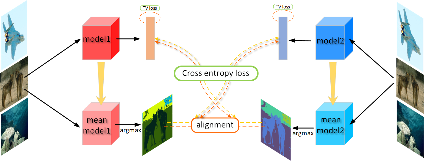Refer to caption — Figure 1: Overall architecture of proposed model for unsupervised image segmentation. (a) is the pipeline of proposed model based on MMT framework. 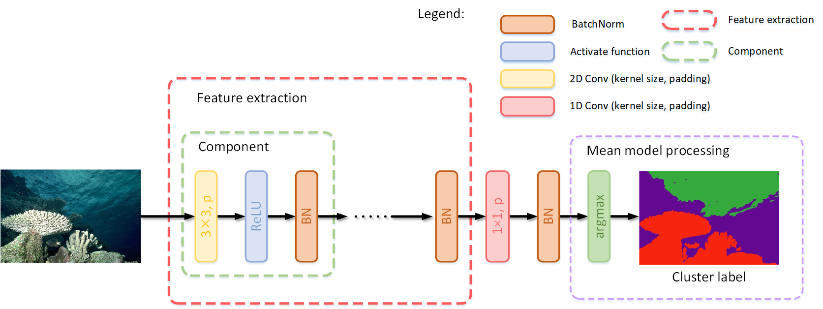It consists of two collaborative networks, model 1 and model 2. They adopt same structure which are optimized under supervisions of off-line refined labels and on-line refined labels.The loss function of total variation and label alignment cross entropy are adopted. (b) is details of model 1 and model 2. It consists of feature extraction module and mean model processing.

Image segmentation can be formulated as a classification problem of pixels with labels. For simplicity, let denote $\{\}^{N}_{n=1}$ unless otherwise noted, where $N$ denotes the number of pixels in an input color image $I=\{x_{n}\in R^{3}\}$ . Let $y_{n}=f(x_{n},\theta)$ simply denote the process of extracting feature, where $\theta$ denotes current network parameters, $f:R^{3}\rightarrow R^{q}$ is a feature extraction function and $\{y_{n}\in R^{q}\}$ be a set of $q$ -dimensional feature vectors of image pixels. Cluster labels $\{c_{n}\in Z\}$ are assigned to all of pixels by $c_{n}=g(y_{n})$ , where $g:R^{q}\rightarrow Z$ denotes a mapping function. $g$ can be an assignment function that return the label of the cluster centroid closest to $y_{n}$ . The details interpretation are found in [13]. A simple method coming our mind, while $f$ and $g$ are fixed, ${c_{n}}$ are obtained using the abovementioned process. Conversely, if $f$ and $g$ are trainable whereas ${c_{n}}$ are specified. then the parameters for $f$ and $g$ in this case can be optimized by gradient descent. Although good results have been achieved in this architecture which meet the following three criteria: Pixels of similar features should be assigned the same label; Spatially continuous pixels should be assigned the same label;The number of unique cluster labels should be large. However, the random initialization of filter parameters in model has crucial influences to the final performance. So how to initialize the filter parameters randomly but also produce stable results ?

we are motivated by the process of MMT creation: conduct label refinery in the target domain by optimizing the neural networks with off-line refined hard pseudo labels and on-line refined soft pseudo labels in a collaborative training manner. They propose this framework for tackling the problem of the label noise affecting the result performance significantly, especially in unsupervised learning. But the disadvantage is that there are fixed number of output label where it not available for our task requirements. So we select cluster label aligning algorithm [22] without fixed number of label instead of using k-means. Our structure is proposed, as shown in Fig. 1.

3.1 Network architecture

In model1, given the input image $x_{n}$ where each pixel value is normalized. The network is trained to extract features transformation function $y_{n}^{1}=f_{1}(x_{n},\theta_{1})$ . Subsequently, to assign each pixel to a label is calculated by $C_{n}^{1}=argmax\{y_{n}^{1},y_{n}\in R^{q}\}$ . Similarly, model2 generates labels by the same networks with different initializations. We denote the feature transformation functions $y_{n}^{2}=f_{2}(x_{n},\theta_{2})$ and denote their corresponding label classifiers as $C_{n}^{2}$ . If this two collaborative networks also generate labels by network predictions for training each other, their labels are lots of noise. In order to mitigate the label noise, the past temporally average model of each network is applied to instead of the current model to generate the labels. Specifically, the parameters of the temporally average models of the two networks at current iteration $T$ are denoted as $\theta_{mean1}^{T}$ and $\theta_{mean2}^{T}$ respectively, which can be calculated as

\theta_{1}^{T}=\theta_{1}^{T-1}+\eta\nabla\theta_{1}

\theta_{2}^{T}=\theta_{2}^{T-1}+\eta\nabla\theta_{2}

\theta_{mean1}^{T}=\alpha\theta_{mean1}^{T-1}+(1-\alpha)\theta_{1}^{T}

\theta_{mean2}^{T}=\alpha\theta_{mean2}^{T-1}+(1-\alpha)\theta_{2}^{T}

where $\theta_{mean1}^{T-1}$ , $\theta_{mean2}^{T-1}$ indicate the temporal average parameters of the two networks in the previous iteration $(T-1)$ ,the initial temporal average parameters are $\theta_{mean1}^{0}=\theta_{1}^{0}$ , $\theta_{mean2}^{0}=\theta_{2}^{0}$ , $\alpha\in[0,1)$ , $\eta$ is learning rate.

However, due to different initialization in the network, there is a great deal of difference between the two label generated by features of each channel in different network. As above assumption that $C_{n}^{1}=\{c_{1}^{1},c_{2}^{1},...,c_{n}^{1}\}$ and $C_{n}^{2}=\{c_{1}^{2},c_{2}^{2},...,c_{n}^{2}\}$ , $C_{n}^{1}$ and $C_{n}^{2}$ is divided into $k$ sorts that can be expressed by the label vector $\lambda^{1}=[\lambda_{1}^{1},\lambda_{2}^{1},...,\lambda_{n}^{1}]$ and $\lambda^{2}=[\lambda_{1}^{2},\lambda_{2}^{2},...,\lambda_{n}^{2}]$ where $\lambda_{i}^{1},\lambda_{i}^{2}\in\{1,2,...,k\}$ are the cluster label from different networks. In order to address the issue of aligning label, the overlap similarity matrix $S$ could be constructed, where $S_{i,j}$ items appear in both $\lambda_{i}^{1}$ and $\lambda_{j}^{2}$ is counted. Then, the pair of clusters whose number of overlapped data items is the largest, are matched in the way that they are denoted by the same label.Such a process is repeated until all the clusters are matched.The programming model is expressed as formula follows.

\max Z=sum\ S\bigodot D_{dec}=\sum_{i=1}^{n}\sum_{j=1}^{n}s_{i,j}\times d_{i,j}

s.t.\ \ \sum_{i=1}^{n}d_{i,j}=1(j=1,2,\dots,n)\\

\sum_{j=1}^{n}d_{i,j}=1(i=1,2,\dots,n)\\

d_{i,j}=0,1\\

where $S$ is overlap similarity matrix, $D_{dec}$ is the decision-making matrix. $\bigodot$ is matrix points multiplication sign.Briefly, we use $h$ denote the process of label alignment,

C_{n}^{2^{\prime}}=h_{2}(C_{n}^{1})

C_{n}^{1^{\prime}}=h_{1}(C_{n}^{2})

where $h_{1}$ denotes the map from the space of $C_{n}^{2}$ to the space of $C_{1}$ and $h_{2}$ denotes the map from the space of $C_{n}^{1}$ to the space of $C_{n}^{2}$ .

Input: I =

x_{n}\in R^{3}

Output:

L=\{c_{n}\in Z\}

Init()\rightarrow\theta_{1},\theta_{2}

; 2

\theta_{1}^{mean1}=\theta_{1},\theta_{2}^{mean2}=\theta_{2}

; 3

for t=2:T do 5

y_{n}^{1}=GetFeats_{1}(x_{n})

; 6

y_{n}^{mean2}=GetFeats_{mean2}(x_{n})

; 7

C_{n}^{mean2}=argmax\{y_{n}^{mean2}\}

; 8

C_{n}^{1^{\prime}}=h_{1}(C_{n}^{mean2})

{LabelAssignment}

; 9

L_{sim}^{1}=L_{sim}(y_{n}^{1},C_{n}^{1^{\prime}})

L_{tv}^{1}=L_{tv}(y_{n}^{1})

; 10

L^{1}=L_{sim}^{1}+\beta L_{tv}^{1}

; 11

\theta_{1}^{t}=\theta_{1}^{t-1}+\eta\nabla\theta_{1}

\theta_{1,mean}^{t}=\alpha\theta_{1,mean}^{t-1}+(1-\alpha)\theta_{1}^{t}

; 12

y_{n}^{2}=GetFeats_{2}(x_{n})

; 13

y_{n}^{mean1}=GetFeats_{mean1}(x_{n})

; 14

C_{n}^{mean1}=argmax\{y_{n}^{mean1}\}

, ; 15

C_{n}^{2^{\prime}}=h_{2}(C_{n}^{mean1})

{LabelAssignment}

; 16

L_{sim}^{2}=L_{sim}(y_{n}^{2},c_{n}^{2^{\prime}})

L_{tv}^{2}=L_{tv}(y_{n}^{2})

; 17

L^{2}=L_{sim}^{2}+\beta L_{tv}^{2}

; 18

\theta_{2}^{t}=\theta_{2}^{t-1}+\eta\nabla\theta_{2}

\theta_{mean2}^{t}=\alpha\theta_{mean2}^{t-1}+(1-\alpha)\theta_{2}^{t}

; 19

Algorithm 1 Unsupervised image segmentation using MMT

3.2 Loss Functions

TV Loss. To encourage the cluster labels to be the same as those of the neighboring pixels. total variation regularizer would be considered to horizontal and vertical differences of output label.we follow prior work [23]. The spatial continuity loss $L_{tv}$ is defined as follows:

L_{tv}(y_{n})=\sum_{i=1}^{W-1}\sum_{j=1}^{H-1}(||y_{i+1,j}-y_{i,j}||_{1}+||y_{i,j+1}-y_{i,j}||_{1})

where $W$ and $H$ represent the width and height of an input image, $||\cdot||_{1}$ represent the $L1-norm$ . whereas $y_{i,j}$ represents the pixel value at $(i,j)$ in the feature map $y$ .

Feature Loss. the cluster labels generated by average model2 are obtained by applying the $argmax$ function to the feature map $y_{mean2}$ . The cluster labels $c^{mean2}_{n}$ are further utilized as the pseudo targets. And then align label with model1 by mapping function of $h_{1}$ . The feature loss penalizes the output label when it deviates in content from the target $C_{n}^{mean2}$ . To achieve this goal, the following cross entropy loss is calculated:

L_{sim}(y_{n},h_{1}(C^{mean2}_{n}))=\\ \sum_{n=1}^{N}\sum_{j=1}^{q}(-\delta(j-h_{1}(C^{mean2}_{n}))\ln{y}^{n,j})

where

\delta(t)=\left\{\begin{array}[]{rcl}1&&{if\quad t=0}\\ 0&&{otherwise}\end{array}\right.

3.3 OVERALL LOSS AND ALGORITHM

To finish the task of image segmentation, we assign label to match the feature content representation of $y_{n}$ and spatial smoothness simultaneously. Thus we jointly minimise the distance of the content feature representations and spatial smoothness. The loss function we minimise is

L_{total}=L_{sim}+\beta L_{tv}

where $\beta$ is the weighting factor for spatial smoothness.

The detailed optimization procedures are summarized in Algorithm 1. Compared to traditional unsupervised algorithm, labels generated by off-line refined instead of the labels generated by on-line algorithm. We keep the model2 and mean model2 constant during the model1 training phase, As model1 training tries to figure out how to segment the image using labels generated by mean model2, and then align the labels of the output of model1 and model2. Immediately, the parameter of $\theta_{1}$ and $\theta_{mean1}$ are updated. Similarly, keep the model1 and mean model1 constant during the model2 training phase. the model2 would be trying to segment image according to labels generated by mean model1. Then the parameter of $\theta_{2}$ and $\theta_{mean2}$ are updated. After several steps of training, if model1,mean model1, model2 and mean model2 have enough capacity, they will reach a point at which four models are stable.

4 EXPERIMENTAL RESULTS

{

Figure 2: Results of proposed method and [12] generated by training three times without fine-tuning any parameters. In first row, the first image is input image. The other three images are image segmentation results with different segments showing in different colors. The second row show three images are generated by our method.

In this section, we conduct experiments to verify the effectiveness of the proposed stable image segmentation approach in unsupervised learning. 200 test images from the Benchmark(BSD500) are chosen to evaluate the proposed method. We trained the proposed model with T = 1000 iterations and fixed q = 100 for the channel of output feature map in the experiments. The number of convolutional layers M was set to 3 and the temporal ensemble momentum $\alpha$ is set to 0.999. The model parameters are optimized by the stochastic gradient descent method (SGD). The learning rate is fixed to 0.1 and set momentum to 0.9.

For the comparison, we reproduce the baseline image segmentation from [12]. Figure 2 shows the better results from our structure. The first row which we repeat training 3 times without fine-tuning any parameters from [13] resulted in poor stable performance. Our method has a significant stable performance improvement.

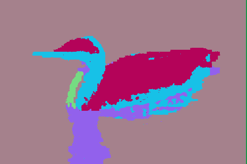
Examples of unsupervised image segmentation results on PASCAL VOC 2012 and BSD500 are shown in Figure 3 and Figure 4, respectively. Figure 3 shows a comparison of five images from the BSD500. The first two rows show the origin images and ground truth image segmentations, and third row shows the predicted image segmentation results with method of [12], which I pick out relatively good results with training many times , and the last row are our results.They also demonstrate that our method performed better and more consistently, which indicates that our model was able to learn features that are stable to a large range of intensity variations.The results of segmentation comparing our method with IIC[24], [12] and [13] are shown in Figure 4. Note that our results in very smooth image segmentation which is closer to ground truth segmentation. The images in Figure 4 offer compelling evidence that our segmentation algorithm performs well on a variety of images from different domains.

The evaluation of segmentation results is that we can compare the segmentations produced by different algorithms, such as the k-means clustering, graph-based segmentation method (GS)[9] , [12] and [13]. The parameters of [12] and [13] are same as the parameter of we proposed method.The best parameters of k-means clustering and graph-based segmentation algorithms were experimentally determined from $\{2,5,8,11,14,17,20\}$ and $\{100,500,1000,1500,2000\}$ . we get a accuracy table from calculating the true positives divided by sample size. The standard protocol of finding the best one-to-one permutation mapping between learned and ground-truth clusters using linear assignment[kuhn2005hungarian]. Table 1 are drawn by calculating an evaluation parameter from BSD500.

Method	Accuracy
Kmeans[8]	0.3639
GS[9]	0.4661
Kanezaki[12]	0.5269
Kim[13]	0.5023
ours	0.5384

Table 1: Comparison pixel accuracy of unsupervised segmentation method in BSD500.

5 Conclusions

In this paper, we proposed a unsupervised image segmentation model based on MMT, and using overlap similarity degree methods for label alignment. The model consists of convolutional filters for feature extraction and differentiable processes for feature clustering, which enables end-to-end network training. We have applied this method to unsupervised image segmentation where we achieve comparable performance and drastically improved stable compared to existing methods.

In future work, we hope to explore the use of other loss functions for unsupervised image segmentation tasks, such as semantic segmentation loss. We also plan to investigate the use of self-attention mechanism to unsupervised image segmentation.

References

[1] M. Everingham, L. Van Gool, C. K. I. Williams, J. Winn, and A. Zisserman. The PASCAL Visual Object Classes Challenge 2012 (VOC2012) Results. http://www.pascal-network.org/challenges/VOC/voc2012/workshop/index.html.
[2] David Martin, Charless Fowlkes, Doron Tal, and Jitendra Malik. A database of human segmented natural images and its application to evaluating segmentation algorithms and measuring ecological statistics. In Proceedings Eighth IEEE International Conference on Computer Vision. ICCV 2001, volume 2, pages 416–423. IEEE, 2001.
[3] Alex Krizhevsky, Ilya Sutskever, and Geoffrey E Hinton. Imagenet classification with deep convolutional neural networks. In Advances in neural information processing systems, pages 1097–1105, 2012.
[4] Karen Simonyan and Andrew Zisserman. Very deep convolutional networks for large-scale image recognition. arXiv preprint arXiv:1409.1556, 2014.
[5] Jonathan Long, Evan Shelhamer, and Trevor Darrell. Fully convolutional networks for semantic segmentation. In Proceedings of the IEEE conference on computer vision and pattern recognition, pages 3431–3440, 2015.
[6] Shuai Zheng, Sadeep Jayasumana, Bernardino Romera-Paredes, Vibhav Vineet, Zhizhong Su, Dalong Du, Chang Huang, and Philip HS Torr. Conditional random fields as recurrent neural networks. In Proceedings of the IEEE international conference on computer vision, pages 1529–1537, 2015.
[7] Vijay Badrinarayanan, Alex Kendall, and Roberto Cipolla. Segnet: A deep convolutional encoder-decoder architecture for image segmentation. IEEE transactions on pattern analysis and machine intelligence, 39(12):2481–2495, 2017.
[8] K Krishna and M Narasimha Murty. Genetic k-means algorithm. IEEE Transactions on Systems, Man, and Cybernetics, Part B (Cybernetics), 29(3):433–439, 1999.
[9] Pedro F Felzenszwalb and Daniel P Huttenlocher. Efficient graph-based image segmentation. International journal of computer vision, 59(2):167–181, 2004.
[10] Liangchen Song, Cheng Wang, Lefei Zhang, Bo Du, Qian Zhang, Chang Huang, and Xinggang Wang. Unsupervised domain adaptive re-identification: Theory and practice. Pattern Recognition, 102:107173, 2020.
[11] Xinyu Zhang, Jiewei Cao, Chunhua Shen, and Mingyu You. Self-training with progressive augmentation for unsupervised cross-domain person re-identification. In Proceedings of the IEEE International Conference on Computer Vision, pages 8222–8231, 2019.
[12] Asako Kanezaki. Unsupervised image segmentation by backpropagation. In 2018 IEEE international conference on acoustics, speech and signal processing (ICASSP), pages 1543–1547. IEEE, 2018.
[13] Wonjik Kim, Asako Kanezaki, and Masayuki Tanaka. Unsupervised learning of image segmentation based on differentiable feature clustering. IEEE Transactions on Image Processing, 29:8055–8068, 2020.
[14] Yixiao Ge, Dapeng Chen, and Hongsheng Li. Mutual mean-teaching: Pseudo label refinery for unsupervised domain adaptation on person re-identification. arXiv preprint arXiv:2001.01526, 2020.
[15] Mircea Cimpoi, Subhransu Maji, and Andrea Vedaldi. Deep filter banks for texture recognition and segmentation. In Proceedings of the IEEE conference on computer vision and pattern recognition, pages 3828–3836, 2015.
[16] Junjun He, Zhongying Deng, and Yu Qiao. Dynamic multi-scale filters for semantic segmentation. In Proceedings of the IEEE/CVF International Conference on Computer Vision (ICCV), October 2019.
[17] Maxime Oquab, Leon Bottou, Ivan Laptev, and Josef Sivic. Learning and transferring mid-level image representations using convolutional neural networks. In Proceedings of the IEEE conference on computer vision and pattern recognition, pages 1717–1724, 2014.
[18] Zhangjie Cao, Mingsheng Long, Jianmin Wang, and Michael I Jordan. Partial transfer learning with selective adversarial networks. In Proceedings of the IEEE Conference on Computer Vision and Pattern Recognition, pages 2724–2732, 2018.
[19] Samuli Laine and Timo Aila. Temporal ensembling for semi-supervised learning. arXiv preprint arXiv:1610.02242, 2016.
[20] Ying Zhang, Tao Xiang, Timothy M Hospedales, and Huchuan Lu. Deep mutual learning. In Proceedings of the IEEE Conference on Computer Vision and Pattern Recognition, pages 4320–4328, 2018.
[21] Haixiong Fan, Fuxian Liu, and Lu Xia. Cluster label aligning algorithm based on programming model. In 2012 24th Chinese Control and Decision Conference (CCDC), pages 1768–1772. IEEE, 2012.
[22] Zhi-Hua Zhou and Wei Tang. Clusterer ensemble. Knowledge-Based Systems, 19(1):77–83, 2006.
[23] Takashi Shibata, Masayuki Tanaka, and Masatoshi Okutomi. Misalignment-robust joint filter for cross-modal image pairs. In Proceedings of the IEEE International Conference on Computer Vision, pages 3295–3304, 2017.
[24] Xu Ji, João F Henriques, and Andrea Vedaldi. Invariant information clustering for unsupervised image classification and segmentation. In Proceedings of the IEEE International Conference on Computer Vision, pages 9865–9874, 2019.