跳到论文正文
W Papers独立论文阅读器 arXiv:2012.08853 论文正文 计算阅读时间 · 0%
引用这篇论文根据当前论文元数据生成,正式投稿前建议核对。


License: arXiv.org perpetual non-exclusive license
arXiv:2012.08853v1 [physics.class-ph] 16 Dec 2020

On the interplay between Noether’s theorem and the theory of adiabatic invariants

Thierry Gourieux    Raphaël Leone Affiliation: Laboratoire de Physique et Chimie Théoriques (UMR CNRS 7019), Université de Lorraine, F-54506 Vandœuvre-lès-Nancy Email: thierry.gourieux@univ-lorraine.fr
Abstract

This article focuses on an important quantity that will be called the Rund-Trautman function. It already plays a central role in Noether’s theorem since its vanishing characterizes a symmetry and leads to a conservation law. The main aim of the paper is to show how, in the realm of classical mechanics, an ‘almost’ vanishing Rund-Trautman function accompanying an ‘almost’ symmetry leads to an ‘almost’ constant of motion within the adiabatic assumption, that is, to an adiabatic invariant. To this end, the Rund-Trautman function is first introduced and analysed in detail, then it is implemented for the general one-dimensional problem. Finally, its relevance in the adiabatic context is examined through the example of the harmonic oscillator with a slowly varying frequency. Notably, for some frequency profiles, explicit expansions of adiabatic invariants are derived through it and an illustrative numerical test is realized.

Keywords: Noether’s theorem, Adiabatic invariants, Classical Mechanics

1 Introduction

It is an understatement to say that, for a century now, Noether’s two theorems [1, 2] have played a central role in physics [3]. Since both symmetry and variational principles have become so fundamental to the point that they structure modern theories, these theorems are nowadays an indispensable part of any syllabus in pure physics. At an advanced level: in gauge theories of which they constitute a cornerstone, but also, beforehand, in analytical mechanics where Noether’s name is generally mentioned for the first time through her first theorem. Indeed, the second theorem objectively plays a marginal role in this framework, though it is not without interest concerning parameter-free variational principles [4] (as Jacobi’s formulation of the principle of least action). The first theorem, for its part, is simply called ‘the theorem of Noether’, and is mostly stated with the principal aim of rederiving the usual conservation laws from invariances of the action under transformations. It has the advantage of gathering all the existing conservation laws under a universal and elegant symmetry principle.

A semester-length course on classical mechanics — which must cover many topics such as calculus of variations, Lagrangian and Hamiltonian mechanics, canonical transformations, the Hamilton-Jacobi equation, action-angle coordinates, and so on, not to mention all the important applications — cannot spend many time on each individual chapter. This is the reason why the first theorem of Noether is rarely treated in more detail. Pedagogical articles on the subject are aimed to fill this gap. One of the most interesting topics is certainly the reversed question about searching for unknown conservation laws in some practical situation, by analysing the symmetries (if any) admitted by the action functional. The method, as described for example in Neuenschwander’s book [5], consists in seeking transformations satisfying the so-called Rund-Trautman identity [6, 7]. That task can generally be achieved in an algorithmic way if we restrict ourselves to point transformations [8, 9, 10].

It is interesting to interpret the Rund-Trautman identity as the identical vanishing of a quantity RR that will be called the Rund-Trautman function in this article. As will be shown, RR turns out to be the rate of change along the motion of both (i) a Noether asymmetricity and (ii) the non conservation of the quantity that would have been conserved in case of symmetry. These properties prove the role that can play RR in the problem of perturbatively finding ‘almost’ conservation laws when a system depends on small parameters. This is the main purpose of the present article regarding the adiabatic hypothesis. Our approach will be elementary enough to avoid complicated mathematical techniques [11].

The paper is organized as follows. We first draw in section 2 a basic portrait of the space of events associated with a mechanical system, and we outline how point transformations act in that space. In section 3 are reviewed the important features of Noether’s first theorem regarding point transformations, including the Rund-Trautman function as well as coordinate and gauge issues. In section 4, we apply the theory to the determination of all the Noether point symmetries of natural one-dimensional problems [12], with an emphasis put on the time-dependent harmonic oscillator. Section 5 is then devoted to the notions of almost symmetries and almost conservation laws within the adiabatic hypothesis. In order to comply with the amusing saying according to which ‘classical mechanics is the art of solving the harmonic oscillator in many ways’, we treat the case of the paradigmatic time-dependent harmonic oscillator [13, 14]. After obtaining a formal expansion of an adiabatic invariant to arbitrary orders, we derive explicit expressions for some frequency profiles and we end the article with a numerical test.

In order to remain as pedagogical as possible without obscuring the main content, all the calculations will be explained and detailed in appendices. Alternatively, they can be considered as exercises for the reader.

2 Continuous point transformations in the space of events

2.1 The space of events and its coordinatizations

Let us take as a starting point a classical mechanical problem whose configuration space 𝒬\mathcal{Q} is an nn-dimensional smooth manifold. Since our framework is Newtonian, there exists independently a timeline 𝒯\mathcal{T}, diffeomorphic to the real line, whose points are the positions in time. The space of events (or extended configuration space) is the Cartesian product ℰ=𝒯×𝒬\mathcal{E}=\mathcal{T}\times\mathcal{Q} usually coordinatized by (1+n)(1+n)-tuples whose first element is the absolute time along 𝒯\mathcal{T}, the nn others being coordinates in 𝒬\mathcal{Q}. However, it might be interesting to consider arbitrary coordinate systems in ℰ\mathcal{E} possibly ‘mixing’ 𝒯\mathcal{T} and 𝒬\mathcal{Q}. Such a system will be generically denoted by (t,q)(t,q) with q=(qi)q=(q^{i}) and i=1,…,ni=1,\dots,n. We must only be sure that tt can play the role of a time along the actual evolution of the configuration point in 𝒬\mathcal{Q}, i.e. that it increases strictly with the absolute time (it is certainly the case if tt is simply a future-oriented coordinate in 𝒯\mathcal{T}, e.g. the absolute time itself). Geometrically, it amounts to say that the curve drawn by the evolution in ℰ\mathcal{E} is, in coordinates, the graph of a mapping 𝒞:t↦q⁡(t)\mathcal{C}\colon t\mapsto q(t). It is often interesting to reduce at least formally the specificity of the time coordinate by setting t≡q0t\equiv q^{0} and (t,q)=(qμ)(t,q)=(q^{\mu}) with μ=0,…,n\mu=0,\dots,n.

2.2 Continuous point transformations

A continuous point transformation Φ\Phi of the space of events is essentially a mechanism which unambiguously maps any event (t,q)(t,q) into a parameter-dependent one, (tε,qε)(t_{\varepsilon},q_{\varepsilon}) say, where ε\varepsilon is the parameter. Locally, it admits a form

(t,q)⟶(tε,qε)=Φ⁡(t,q,ε)=(t+ε​τ​(t,q),q+ε​ξ​(t,q))+O⁡(ε2),(t,q)\longrightarrow(t_{\varepsilon},q_{\varepsilon})=\Phi(t,q;\varepsilon)=\big(t+\varepsilon\tau(t,q),q+\varepsilon\xi(t,q)\big)+\mathrm{O}(\varepsilon^{2}), (1)

in some vicinity of ε=0\varepsilon=0, the quantities τ\tau and ξ=(ξi)\xi=(\xi^{i}) being smooth functions of their arguments. The transformation Φ\Phi is entirely characterized and generated by the vector field [15]

𝖷=τ∂∂t+ξi∂∂qi=ξμ∂μ(ξ0≡τ,∂μ≡∂∂qμ)\mathsf{X}=\tau\,\frac{\partial}{\partial t}+\xi^{i}\frac{\partial}{\partial q^{i}}=\xi^{\mu}\partial_{\mu}\qquad\Bigg(\xi^{0}\equiv\tau\;,\;\partial_{\mu}\equiv\frac{\partial}{\partial q^{\mu}}\Bigg)

on ℰ\mathcal{E}, the Einstein summation convention being assumed in this paper (Latin and Greek indices cover the ranges 1,…,n1,\dots,n and 0,…,n0,\dots,n respectively). It is the vector field which has for components the nn-tuple (ξμ)(\xi^{\mu}) with respect to the coordinate system (qμ)(q^{\mu}).

Actually, Φ\Phi drags the events along the integral curves of 𝖷\mathsf{X}. From now on, ε\varepsilon will be considered as an infinitesimal and any term of order higher than the first in ε\varepsilon will be neglected. This way, ε​𝖷\varepsilon\mathsf{X} is the infinitesimal translation bringing the original event (t,q)(t,q) to the transformed one (tε,qε)(t_{\varepsilon},q_{\varepsilon}).

2.3 Induced transformations and symmetries of point functions

Let F0F_{0} be a smooth point function11 1 The French mathematician Gabriel Lamé called ‘fonction-de-point’ a real-valued function defined on the ‘absolute space’ under consideration (originally the three-dimensional physical space) [16]. It unambiguously associates a real value to any point of that space and can secondarily acquire an analytical expression through a coordinate system. It is a basic example of scalar. defined on ℰ\mathcal{E}. Applying a first-order Taylor expansion based on (1), while (t,q)(t,q) is mapped into (tε,qε)(t_{\varepsilon},q_{\varepsilon}), the value of F0F_{0} undergoes the transformation

F0​(t,q)⟶F0​(tε,qε)=F0​(t,q)+ε​𝖷​(F0)​(t,q).F_{0}(t,q)\longrightarrow F_{0}(t_{\varepsilon},q_{\varepsilon})=F_{0}(t,q)+\varepsilon\mathsf{X}(F_{0})(t,q). (2)

One says that Φ\Phi is a symmetry of F0F_{0} if it leaves its values invariant in the flow of Φ\Phi, i.e. if the variation of F0F_{0} is everywhere zero in the direction of 𝖷\mathsf{X}. This is the case if and only if (iff) 𝖷⁡(F0)\mathsf{X}(F_{0}) vanishes identically. Geometrically, it means that the field 𝖷\mathsf{X} is tangent to the level surfaces of F0F_{0} (or equivalently that the integral curves of 𝖷\mathsf{X} are contained in these surfaces).

-2.1,-0.7)(2.2,2.4) psaxes[labelFontSize=,xAxis=true,yAxis=true,labels=none,ticks=none]-¿(-0.0,-.3)(-2.1,-0.5)(2.,2.) psplot[plotpoints=200,linestyle=dashed,dash=2pt 2pt]-21.552.718281828459045 ( -x ( 2.0))+0.1 psplot[plotpoints=200]-1.81.81.2*2.718281828459045 ( -(x-0.4) ( 2.0)+0.2)+0.2

Figure 1: Under the action of Φ\Phi, and for sufficiently small values of |ε||\varepsilon|, the original evolution 𝒞\mathcal{C} (dashed line) is mapped into a neighbouring evolution 𝒞ε\mathcal{C}_{\varepsilon} (solid line). The vector ε​𝖷\varepsilon\mathsf{X} is the first order approximation in ε\varepsilon of the transformation (ε\varepsilon is taken positive in the figure).

2.4 Induced transformations of evolutions and their kinematic properties

Now, let t↦q⁡(t)t\mapsto q(t) be a generic smooth evolution of the configuration between two extremities of time t=t1t=t_{1} and t=t2t=t_{2}. As illustrated in figure 1, for sufficiently small values of |ε||\varepsilon|, its graph 𝒞\mathcal{C} drawn in ℰ\mathcal{E} is transformed by Φ\Phi into the graph of another evolution 𝒞ε\mathcal{C}_{\varepsilon} between t=t1​εt=t_{1\varepsilon} and t=t2​εt=t_{2\varepsilon}, according to (see A.1)

(t,q⁡(t))⟶(tε,qε​(tε))=(t+ε​τ​(t,q⁡(t)),q⁡(t)+ε​ξ​(t,q⁡(t))).(t,q(t))\longrightarrow(t_{\varepsilon},q_{\varepsilon}(t_{\varepsilon}))=(t+\varepsilon\tau(t,q(t)),q(t)+\varepsilon\xi(t,q(t))). (3)

Then, the velocity q˙​(t)\dot{q}(t) of the original evolution at t=tt=t becomes the velocity q˙ε​(tε)\dot{q}_{\varepsilon}(t_{\varepsilon}) of the transformed evolution at t=tεt=t_{\varepsilon}. Viewing tεt_{\varepsilon} and qε​(tε)q_{\varepsilon}(t_{\varepsilon}) as functions of the original value tt of the time through the equality in Equation (3), one has

q˙εi​(tε)=d​qεi​(tε)d​tε=d​qεi​(tε)d​t/d​tεd​t,\dot{q}^{i}_{\varepsilon}(t_{\varepsilon})=\frac{{\mathrm{d}}q^{i}_{\varepsilon}(t_{\varepsilon})}{{\mathrm{d}}t_{\varepsilon}}=\frac{{\mathrm{d}}q^{i}_{\varepsilon}(t_{\varepsilon})}{{\mathrm{d}}t}\Bigg/\penalty\frac{{\mathrm{d}}t_{\varepsilon}}{{\mathrm{d}}t}\,, (4)

that is, to the first order in ε\varepsilon (see A.2) :

q˙εi​(tε)=q˙i​(t)+ε⁡[d​ξi​(t,q⁡(t))d​t−q˙i​(t)​d​τ​(t,q⁡(t))d​t].\dot{q}^{i}_{\varepsilon}(t_{\varepsilon})=\dot{q}^{i}(t)+\varepsilon\Bigg[\frac{{\mathrm{d}}\xi^{i}(t,q(t))}{{\mathrm{d}}t}-\dot{q}^{i}(t)\frac{{\mathrm{d}}\tau(t,q(t))}{{\mathrm{d}}t}\Bigg]. (5)

In brief, the formal transformation rules of the time, position and velocity are thus

t⟶tε=t+ε​τ,q⟶qε=q+ε​ξ,q˙⟶q˙ε=q˙+ε⁡(ξ˙−q˙​τ˙).t\longrightarrow t_{\varepsilon}=t+\varepsilon\tau\,,\qquad q\longrightarrow q_{\varepsilon}=q+\varepsilon\xi\,,\qquad\dot{q}\longrightarrow\dot{q}_{\varepsilon}=\dot{q}+\varepsilon(\dot{\xi}-\dot{q}\dot{\tau}).

One could also determine the transformation rules of higher total tt-derivatives of qq in a recursive way, if needed.

2.5 Induced transformations and symmetries of kinematic functions

According to the above transformation rules, while the triple (t,q,q˙)(t,q,\dot{q}) is transformed into (tε,qε,q˙ε)(t_{\varepsilon},q_{\varepsilon},\dot{q}_{\varepsilon}) by Φ\Phi along an evolution, the value of a smooth kinematic function F1F_{1} of the time, position, and velocity, undergoes the transformation

F1​(t,q,q˙)⟶F1​(tε,qε,q˙ε)=F1​(t,q,q˙)+ε​𝖷[1]​(F1)​(t,q,q˙),F_{1}(t,q,\dot{q})\longrightarrow F_{1}(t_{\varepsilon},q_{\varepsilon},\dot{q}_{\varepsilon})=F_{1}(t,q,\dot{q})+\varepsilon\mathsf{X}^{[1]}(F_{1})(t,q,\dot{q}),

where

𝖷[1]=τ​∂∂t+ξi​∂∂qi+(ξ˙i−q˙i​τ˙)​∂∂q˙i\mathsf{X}^{[1]}=\tau\,\frac{\partial}{\partial t}+\xi^{i}\frac{\partial}{\partial q^{i}}+(\dot{\xi}^{i}-\dot{q}^{i}\dot{\tau})\frac{\partial}{\partial\dot{q}^{i}} (6)

is the so-called first prolongation [15] of 𝖷\mathsf{X} especially built to act upon such functions. Here again, the transformation is a symmetry of F1F_{1} if it leaves invariant the values of that function, i.e. if 𝖷[1]​(F1)\mathsf{X}^{[1]}(F_{1}) vanishes identically. One could also prolong 𝖷\mathsf{X} to deal with kinematic functions depending on q¨\ddot{q} and possibly higher total tt-derivatives of qq. However, it will not be necessary for our purpose.

2.6 Adapted coordinate systems

0.05,0.)(15.3,8.95) parametricplot[linewidth=.3pt,linecolor=red]1.70931141844558442.6964645570354881*4.71*cos(t)+0*4.71*sin(t)+4.94—0*4.71*cos(t)+1*4.71*sin(t)+-0.38 parametricplot[linewidth=.3pt,linecolor=red]1.6513582828089842.67436184327952061*3.5*cos(t)+0*3.5*sin(t)+4.63—0*3.5*cos(t)+1*3.5*sin(t)+-0.94 parametricplot[linewidth=.3pt,linecolor=red]1.72356743775388322.7187414143083791*5.72*cos(t)+0*5.72*sin(t)+9.88—0*5.72*cos(t)+1*5.72*sin(t)+3.18 parametricplot[linewidth=.3pt,linecolor=red]1.4729079488704052.9491135499713981*3.37*cos(t)+0*3.37*sin(t)+10.26—0*3.37*cos(t)+1*3.37*sin(t)+4.11 parametricplot1.74485089601768782.97436399643007831*3.26*cos(t)+0*3.26*sin(t)+5.02—0*3.26*cos(t)+1*3.26*sin(t)+4.47 parametricplot-0.361429318218728041.2936873051909431*2.19*cos(t)+0*2.19*sin(t)+10.49—0*2.19*cos(t)+1*2.19*sin(t)+5.42

Figure 2: Schematic illustration of the vector field 𝖷\mathsf{X} over ℰ\mathcal{E} and its representatives with respect to an arbitrary coordinate system (qμ)(q^{\mu}) and an adapted one (qμ¯)(q^{\bar{\mu}}). In the latter, the integral curves of 𝖷\mathsf{X} coincide with the coordinate lines of qα¯q^{\bar{\alpha}}.

For obvious practical reasons, once we have chosen a coordinate system (qμ)(q^{\mu}), each individual coordinate qμq^{\mu} is tacitly identified with the μ\mu-th coordinate function which maps events to their value of qμq^{\mu}. From the transformation (1) regarding the coordinates (which formally reads qμ→qμ+ε​ξμq^{\mu}\to q^{\mu}+\varepsilon\xi^{\mu}), and from the general transformation rule (2) of the point functions, one readily deduces that applying 𝖷\mathsf{X} to the coordinate functions qμq^{\mu} yields the equalities 𝖷⁡(qμ)=ξμ\mathsf{X}(q^{\mu})=\xi^{\mu}. This observation allows us to write the components of 𝖷\mathsf{X} in an arbitrary system (qμ)(q^{\mu}) as (ξμ)=(𝖷⁡(qμ))(\xi^{\mu})=(\mathsf{X}(q^{\mu})). In another system (qμ′)(q^{\mu^{\prime}}) they will be (ξμ′)=(𝖷⁡(qμ′))(\xi^{\mu^{\prime}})=(\mathsf{X}(q^{\mu^{\prime}})), that is, (ξμ′)=(ξν​∂νqμ′)(\xi^{\mu^{\prime}})=(\xi^{\nu}\partial_{\nu}q^{\mu^{\prime}}). This last equality encodes, as expected, the contravariant transformation rule of the components of vector fields.

According to the elementary theory of differential geometry [17], it is always possible to define an extended coordinate system (qμ¯)(q^{\bar{\mu}}) reducing the transformation Φ\Phi to a mere rigid translation of magnitude ε\varepsilon along one of the coordinates, qα¯q^{\bar{\alpha}} say (see figure 2). In such a system which is said to be adapted to Φ\Phi, the total derivatives of the coordinates qi¯q^{\bar{i}} with respect to t¯=q0¯\bar{t}=q^{\bar{0}} remain invariant at all orders, thus 𝖷\mathsf{X} and its prolongations simply coincide with the partial derivative ∂α¯\partial_{\bar{\alpha}}. Hence, saying that Φ\Phi is a symmetry of a point or kinematic function FF amounts to saying that FF does not depend on the coordinate qα¯q^{\bar{\alpha}} in the adapted system (although it may depend on its total derivatives with respect to t¯\bar{t} if qα¯≠t¯q^{\bar{\alpha}}\neq\bar{t}). Alternatively stated, that kind of symmetry allows to reduce by one the number of variables necessary to describe FF.

3 Noether’s theory and the Rund-Trautman function

3.1 Introduction of the Rund-Trautman function

Suppose that the dynamics of the system derives from the Hamilton’s principle applied to an action functional [18]

S⁡(𝒞)=∫t1t2L⁡[q⁡(t)]​𝑑t,S(\mathcal{C})=\int_{t_{1}}^{t_{2}}L[q(t)]\,{\mathrm{d}}t,

where LL is a a smooth Lagrangian of the first order and [q⁡(t)][q(t)] a shorthand notation for the triple of arguments (t,q​(t),q˙​(t))(t,q(t),\dot{q}(t)). It amounts to say that the motions are the evolutions satisfying the Euler-Lagrange equations

𝖤i​(L)=0(i=1,…,n)\mathsf{E}_{i}(L)=0\qquad(i=1,\dots,n)

where

𝖤i=∂∂qi−dd​t​∂∂q˙i\mathsf{E}_{i}=\frac{\partial}{\partial q^{i}}-\frac{{\mathrm{d}}}{{\mathrm{d}}t}\frac{\partial}{\partial\dot{q}^{i}} (7)

is the ii-th Euler-Lagrange operator with respect to the used coordinate system.

Under Φ\Phi, the value of the action transforms as

S⁡(𝒞)⟶S⁡(𝒞ε)\displaystyle S(\mathcal{C})\longrightarrow S(\mathcal{C}_{\varepsilon}) =∫t1​εt2​εL⁡[qε​(tε)]​d​tε\displaystyle=\int_{t_{1\varepsilon}}^{t_{2\varepsilon}}L[q_{\varepsilon}(t_{\varepsilon})]\,{\mathrm{d}}t_{\varepsilon}\, (8)

where [qε​(tε)][q_{\varepsilon}(t_{\varepsilon})] stands for the triple of arguments (tε,qε​(tε),q˙ε​(tε))(t_{\varepsilon},q_{\varepsilon}(t_{\varepsilon}),\dot{q}_{\varepsilon}(t_{\varepsilon})). To the first order in ε\varepsilon, the induced variation of the action is (see B.1)

δ​S​(𝒞)=S⁡(𝒞ε)−S⁡(𝒞)=ε​∫t1t2(𝖷[1]​(L)+τ˙​L)​[q⁡(t)]​𝑑t.\delta S(\mathcal{C})=S(\mathcal{C}_{\varepsilon})-S(\mathcal{C})=\varepsilon\int_{t_{1}}^{t_{2}}\bigg(\mathsf{X}^{[1]}(L)+\dot{\tau}L\bigg)[q(t)]\,{\mathrm{d}}t. (9)

Now, let us introduce some smooth point function BB (given up to a meaningless additive constant) and contemplate the difference

𝒟⁡(𝒞)=[ε​B​(t,q⁡(t))]t1t2−δ​S​(𝒞)=ε​∫t1t2R⁡[q⁡(t)]​𝑑t,\mathcal{D}(\mathcal{C})=\Big[\varepsilon B(t,q(t))\Big]_{t_{1}}^{t_{2}}-\delta S(\mathcal{C})=\varepsilon\int_{t_{1}}^{t_{2}}R[q(t)]\,{\mathrm{d}}t, (10)

where has been introduced the kinematic function

R⁡(t,q,q˙)=B˙−𝖷[1]​(L)−τ˙​LR(t,q,\dot{q})=\dot{B}-\mathsf{X}^{[1]}(L)-\dot{\tau}L (11)

that will be called the Rund-Trautman function defined by the Lagrangian LL, the transformation Φ\Phi and the boundary term BB. Rearranging its right-hand side (see B.2), the last equation can be rewritten

R=I˙−(ξi−q˙i​τ)​𝖤i​(L),R=\dot{I}-(\xi^{i}-\dot{q}^{i}\tau)\mathsf{E}_{i}(L), (12)

where was introduced the quantity

I⁡(t,q,q˙)=B+H​τ−pi​ξi=B−pμ​ξμ,I(t,q,\dot{q})=B+H\tau-p_{i}\xi^{i}=B-p_{\mu}\xi^{\mu}, (13)

with pi=∂L/∂q˙ip_{i}=\partial L/\partial{\dot{q}^{i}} and p0=−H=L−pi​q˙ip_{0}=-H=L-p_{i}\dot{q}^{i} the components of the extended momentum. From (12), one sees that RR is the rate of change of II along the motions.

The fact that the left-hand side of (10) has a coordinate-free meaning suffices to say that R​d​tR{\mathrm{d}}t in the right-hand side is invariant under a change of extended coordinates. It is also the case of II since BB and the contraction pμ​ξμp_{\mu}\xi^{\mu} are scalars.

3.2 Harmonization with the Lagrangian gauge freedom

One knows that the dynamics is invariant under the addition of a total differential d​G{\mathrm{d}}G to the form L​d​tL{\mathrm{d}}t, where GG is a point function. This addition corresponds to the gauge transformation L→L~=L+G˙L\to\widetilde{L}=L+\dot{G} of the Lagrangian. Accordingly, the action gauge-transforms as

S⁡(𝒞)⟶S~​(𝒞)=∫t1t2L~​[q⁡(t)]​𝑑t=S⁡(𝒞)+[G⁡(t,q⁡(t))]t1t2S(\mathcal{C})\longrightarrow\widetilde{S}(\mathcal{C})=\int_{t_{1}}^{t_{2}}\widetilde{L}[q(t)]\,{\mathrm{d}}t=S(\mathcal{C})+\Big[G(t,q(t))\Big]_{t_{1}}^{t_{2}}

and its variation under Φ\Phi as

δ​S​(𝒞)⟶δ​S~​(𝒞)=S~​(𝒞ε)−S~​(𝒞).\delta S(\mathcal{C})\longrightarrow\delta\widetilde{S}(\mathcal{C})=\widetilde{S}(\mathcal{C}_{\varepsilon})-\widetilde{S}(\mathcal{C}).

As is shown in B.3, one obtains, to the first order in ε\varepsilon:

δ​S~​(𝒞)=δ​S​(𝒞)+ε​[𝖷⁡(G)​(t,q⁡(t))]t1t2.\delta\widetilde{S}(\mathcal{C})=\delta S(\mathcal{C})+\varepsilon\,\Big[\mathsf{X}(G)(t,q(t))\Big]_{t_{1}}^{t_{2}}\,. (14)

The difference 𝒟⁡(𝒞)\mathcal{D}(\mathcal{C}) is rendered gauge-invariant if one endows with BB the compensating gauge transformation law

B⟶B~=B+𝖷⁡(G).B\longrightarrow\widetilde{B}=B+\mathsf{X}(G).

Indeed, it is easily verified that

[ε​B~​(t,q⁡(t))]t1t2−δ​S~​(𝒞)=[ε​B​(t,q⁡(t))]t1t2−δ​S​(𝒞).\Big[\varepsilon\widetilde{B}(t,q(t))\Big]_{t_{1}}^{t_{2}}-\delta\widetilde{S}(\mathcal{C})=\Big[\varepsilon B(t,q(t))\Big]_{t_{1}}^{t_{2}}-\delta S(\mathcal{C}).

Consequently, the Rund-Trautman function is gauge invariant (R~=R\widetilde{R}=R), as well as II, according to the gauge transformation rule of the extended momenta:

I~=B~−p~μ​ξμ=B~−(pμ+∂μG)​ξμ=B~−pμ​ξμ−𝖷⁡(G)=B−pμ​ξμ=I.\widetilde{I}=\widetilde{B}-\tilde{p}_{\mu}\xi^{\mu}=\widetilde{B}-(p_{\mu}+\partial_{\mu}G)\xi^{\mu}=\widetilde{B}-p_{\mu}\xi^{\mu}-\mathsf{X}(G)=B-p_{\mu}\xi^{\mu}=I.

3.3 Trivialization of the formalism through adapted gauge and coordinates

Locally, one can always choose a point function GG verifying the gauge condition B+𝖷⁡(G)=0B+\mathsf{X}(G)=0 in order to cancel the boundary term. Such a gauge will be said to be adapted to the couple formed by the transformation and the boundary term. It can be most easily done by using an adapted coordinate system (qμ¯)=(t¯,qi¯)(q^{\bar{\mu}})=(\bar{t},q^{\bar{i}}) such that 𝖷=∂α¯\mathsf{X}=\partial_{\bar{\alpha}}. Indeed, the gauge condition becomes B+∂α¯G=0B+\partial_{\bar{\alpha}}G=0 and an integral of this expression with respect to qα¯q^{\bar{\alpha}} suffices to obtain a suitable point function GG.

Once this is done, the Lagrangian L¯\overline{L} expressed in the adapted system and defined by L¯​d​t¯=L​d​t+d​G\overline{L}{\mathrm{d}}\bar{t}=L{\mathrm{d}}t+{\mathrm{d}}G is given in an adapted gauge as well. The Rund-Trautman function is now simply R¯=−∂α¯L¯\overline{R}=-\partial_{\bar{\alpha}}\overline{L} and II reduces to

I=−p¯α¯=−∂L¯∂q̊α¯,I=-\overline{p}_{\bar{\alpha}}=-\frac{\partial\overline{L}}{\partial\mathring{q}^{\bar{\alpha}}}\,,

where, in order to avoid any confusion, the empty bullet symbolizes the derivation with respect to the adapted time t¯\bar{t}. Hence, equation (12) becomes, along the motions, tantamount to the Euler-Lagrange equation 𝖤α¯​(L¯)=0\mathsf{E}_{\bar{\alpha}}(\overline{L})=0. Actually, R¯\overline{R} measures the dependence of the adapted Lagrangian L¯\overline{L} on qα¯q^{\bar{\alpha}} as well as the rate of change of the momentum p¯α¯\overline{p}_{\bar{\alpha}} along the motions (up to a sign).

3.4 Symmetry or not symmetry

One says that the transformation Φ\Phi is a Noether point symmetry (NPS) of the problem if there exists a boundary term BB such that 𝒟⁡(𝒞)\mathcal{D}(\mathcal{C}) vanishes for any evolution 𝒞\mathcal{C}. In this case, RR identically vanishes and thus the quantity II is conserved along the motions. According to Paragraph 3.2, an NPS is as expected a gauge-invariant property generating a gauge-invariant constant of motion. In particular, an NPS leaves the action integral invariant in an adapted gauge and the symmetry is said to be strict in this case.

If Φ\Phi is an NPS then its meaning becomes transparent as seen through the lens of the adapted Lagrangian L¯\overline{L} introduced in Paragraph 3.3. Indeed, it says that qα¯q^{\bar{\alpha}} is a cyclic coordinate22 2 In addition, pα¯p_{\bar{\alpha}} being a partial derivative of L¯\overline{L}, it does not depend on qα¯q^{\bar{\alpha}} either. This point demonstrates that an NPS Φ\Phi is a symmetry of the constant of motion II., or equivalently that its conjugate momentum is conserved.

In general, however, RR is interpretable as the rates of change of both the ‘asymmetricity’ and II. Therefore, seeking ‘almost’ vanishing Rund-Trautman functions can be a good approach to find ‘almost’ conserved quantities. In the adiabatic context, the almostness in question will become clearer in Section 4. But, before, we apply the theory discussed in this section to the general one-dimensional Lagrangian problems.

4 Application to one-dimensional problems

4.1 General aspects

We consider in this section the standard Lagrangian of a unit-mass particle experiencing a potential V⁡(t,q)V(t,q) along a straight line:

L=12​q˙2−V⁡(t,q).L=\frac{1}{2}\,\dot{q}^{2}-V(t,q).

Let us introduce the generator 𝖷=τ∂t+ξ∂q\mathsf{X}=\tau\partial_{t}+\xi\partial_{q} of a point transformation Φ\Phi as well as a boundary term BB. The corresponding Rund-Trautman function (11) takes the form

R=R3​(t,q)​q˙3+R2​(t,q)​q˙2+R1​(t,q)​q˙+R0​(t,q),R=R_{3}(t,q)\dot{q}^{3}+R_{2}(t,q)\dot{q}^{2}+R_{1}(t,q)\dot{q}+R_{0}(t,q),

where

R3=12​∂qτ,R2=12​∂tτ−∂qξ,R1=∂qB+V​∂qτ−∂tξ,R0=∂t(B+τ​V)+ξ​∂qV.\begin{array}[]{ll}R_{3}=\displaystyle\frac{1}{2}\,\partial_{q}\tau,&R_{2}=\displaystyle\frac{1}{2}\,\partial_{t}\tau-\partial_{q}\xi,\\ R_{1}=\partial_{q}B+V\partial_{q}\tau-\partial_{t}\xi,&R_{0}=\partial_{t}(B+\tau V)+\xi\partial_{q}V.\end{array} (15)

The three quantities R3R_{3}, R2R_{2} and R1R_{1}, taken in this order, are found to identically vanish iff τ\tau, ξ\xi and BB have the form

τ=τ⁡(t),ξ=12​τ˙​(t)​q+ψ⁡(t),B=14​τ¨​(t)​q2+ψ˙​(t)​q+χ⁡(t),\begin{array}[]{ll}\tau=\tau(t),&\xi=\displaystyle\frac{1}{2}\,\dot{\tau}(t)q+\psi(t),\\ B=\displaystyle\frac{1}{4}\,\ddot{\tau}(t)q^{2}+\dot{\psi}(t)q+\chi(t),\end{array} (16)

whatever VV may be. From now on, τ\tau, ξ\xi and BB have these forms in which the three functions τ⁡(t)\tau(t), ψ⁡(t)\psi(t) and χ⁡(t)\chi(t) are arbitrary but fixed. Therefore, the Rund-Trautman function RR reduces to the point function R0R_{0}.

We will restrict ourselves to the case τ≠0\tau\neq 0, i.e. to asynchronous transformations. Reversing Φ\Phi if necessary, one can suppose the transformation future-oriented (τ>0\tau>0) without loss of generality. It is shown in C.1 that the change of extended coordinates (t,q)→(T,Q)(t,q)\to(T,Q), with

T=∫td​tτandQ=qτ−∫tψτ3/2​𝑑t,T=\int^{t}\frac{{\mathrm{d}}t}{\tau}\qquad\text{and}\qquad Q=\frac{q}{\sqrt{\tau}}-\int^{t}\frac{\psi}{\tau^{3/2}}\,{\mathrm{d}}t, (17)

reduces Φ\Phi to the translation (T,Q)→(T+ε,Q)(T,Q)\to(T+\varepsilon,Q), and its generator 𝖷\mathsf{X} to ∂T\partial_{T}. Using the adapted coordinates, one obtains after some straightforward but lengthy calculations (see C.2), that the expression of R0R_{0} in (24yai) is equivalent to the existence of a function W⁡(Q)W(Q) such that

V=1ρ2​W​(Q)−ρ¨2​ρ​q2−1ρ​d⁡(ρ2​α˙)d​t​q+β+1ρ2​∫Tρ2​R0​d​T′,V=\frac{1}{\rho^{2}}\,W(Q)-\frac{\ddot{\rho}}{2\rho}\,q^{2}-\frac{1}{\rho}\frac{{\mathrm{d}}(\rho^{2}\dot{\alpha})}{{\mathrm{d}}t}\,q+\beta+\frac{1}{\rho^{2}}\int^{T}\hskip-2.84526pt\rho^{2}R_{0}\,{\mathrm{d}}T^{\prime}, (18)

where

ρ=τ,α=∫tψτ3/2dtandβ=ψ22​τ2−χτ\rho=\sqrt{\tau}\,,\qquad\alpha=\int^{t}\frac{\psi}{\tau^{3/2}}\,{\mathrm{d}}t\qquad\text{and}\qquad\beta=\frac{\psi^{2}}{2\tau^{2}}-\frac{\chi}{\tau} (19)

are functions of the time only. The function W⁡(Q)W(Q) is defined up to a meaningless additive constant since an alteration W⁡(Q)→W⁡(Q)+cst.W(Q)\to W(Q)+\text{cst.} can be compensated by a redefinition of χ\chi through χ→χ+cst\chi\to\chi+\text{cst}. Actually, χ\chi has no physical meaning, its role is only to ensure the gauge symmetry according to which adding to the potential an explicit function of the time only does not affect the dynamics.

Now, it is shown in C.3 that the gauge condition B+𝖷⁡(G)=0B+\mathsf{X}(G)=0 is fulfilled if one chooses

G=−ρ˙2​ρ​q2−ρ​α˙​q+∫t(12​ρ2​α˙2+β)​𝑑t.G=-\frac{\dot{\rho}}{2\rho}\,q^{2}-\rho\dot{\alpha}q+\int^{t}\Bigg(\frac{1}{2}\,\rho^{2}\dot{\alpha}^{2}+\beta\Bigg){\mathrm{d}}t. (20)

Then, following the method described in Paragraph 3.3 (see C.4), one obtains the adapted Lagrangian

L¯​(T,Q,Q̊)=12​Q̊2−W⁡(Q)−∫Tρ2​R0​𝑑T,\overline{L}(T,Q,\mathring{Q})=\frac{1}{2}\,\mathring{Q}^{2}-W(Q)-\int^{T}\hskip-2.84526pt\rho^{2}R_{0}\,{\mathrm{d}}T, (21)

where the empty bullet symbolizes the total derivation with respect to the new time TT. The integrand of the indefinite integral in (21) is actually the new Rund-Trautman function and is, as expected, the opposite of the partial derivative of the new Lagrangian with respect to TT. Moreover, the new energy function coincides with II:

I=H¯=12​Q̊2+W⁡(Q)+∫Tρ2​R0​𝑑T.I=\overline{H}=\frac{1}{2}\,\mathring{Q}^{2}+W(Q)+\int^{T}\hskip-2.84526pt\rho^{2}R_{0}\,{\mathrm{d}}T.

From the above discussion, we deduce that the variational problem admits asynchronous NPS (ANPS) iff the potential can be written in a form

V=1ρ2​W​(qρ−α)−ρ¨2​ρ​q2−1ρ​d⁡(ρ2​α˙)d​t​q+β,V=\frac{1}{\rho^{2}}\,W\Bigg(\frac{q}{\rho}-\alpha\Bigg)-\frac{\ddot{\rho}}{2\rho}\,q^{2}-\frac{1}{\rho}\frac{{\mathrm{d}}(\rho^{2}\dot{\alpha})}{{\mathrm{d}}t}\,q+\beta, (22)

with ρ>0\rho>0, α\alpha and β\beta three functions of the time. In this case, by inverting the equalities (19) one constructs the functions τ\tau, ψ\psi, χ\chi which define, through (16), the vector field of the ANPS along with the boundary term. In the adapted coordinates (17), the problem is transformed into the conservative problem of a particle experiencing a time-independent potential WW. In this new viewpoint, all becomes transparent: the symmetry (TT-invariance) and the first integral (the new energy).

4.2 Noether point symmetries of quadratic potentials

Let us apply the above considerations to the frequently encountered quadratic potentials

V=12​a​(t)​q2+b⁡(t)​q,V=\frac{1}{2}\,a(t)q^{2}+b(t)q, (23)

where a⁡(t)a(t) and b⁡(t)b(t) are some functions of the time. Since the adapted coordinate QQ is necessarily linear in qq, the only candidates to the function W⁡(Q)W(Q) in (22) have clearly the form

W⁡(Q)=12​C2​Q2+C1​Q+C0,W(Q)=\frac{1}{2}\,C_{2}Q^{2}+C_{1}Q+C_{0}\,,

where C2C_{2}, C1C_{1} and C0C_{0} are constants. Now, substituting W⁡(Q)W(Q) in (22) by the above expression and identifying the result with (23), one obtains that ρ>0\rho>0, α\alpha and β\beta must verify

ρ3​(ρ¨+a​ρ)\displaystyle\rho^{3}(\ddot{\rho}+a\rho) =\displaystyle= C2,\displaystyle C_{2}\,, (24a)
ρ3​[d2d​t2​(α​ρ)+a​α​ρ+b]\displaystyle\rho^{3}\bigg[\frac{{\mathrm{d}}^{2}}{{\mathrm{d}}t^{2}}\big(\alpha\rho\big)+a\alpha\rho+b\bigg] =\displaystyle= C1,\displaystyle C_{1}\,, (24b)
β​ρ2+12​C2​α2−C1​α\displaystyle\beta\rho^{2}+\frac{1}{2}\,C_{2}\alpha^{2}-C_{1}\alpha =\displaystyle= C0.\displaystyle C_{0}\,. (24c)

Fixing the three constants in the right-hand sides at arbitrary values, any solution of the differential equations eq. 24a gives an ANPS with its boundary term. Actually, the system of equations eq. 24a says that the left-hand sides must be constant, i.e. that their derivatives are zero. Differentiating them, one obtains

14𝜏…+aτ˙+12a˙τ\displaystyle\frac{1}{4}\,{\mathop{\kern 0.0pt\tau}\limits^{\vbox to-1.4pt{\kern-2.0pt\hbox{...}\vss}}}+a\dot{\tau}+\frac{1}{2}\,\dot{a}\tau =\displaystyle= 0,\displaystyle 0, (24ya)
ψ¨+a​ψ+32​b​τ˙+b˙​τ\displaystyle\ddot{\psi}+a\psi+\frac{3}{2}\,b\dot{\tau}+\dot{b}\tau =\displaystyle= 0,\displaystyle 0, (24yb)
χ˙+b​ψ\displaystyle\dot{\chi}+b\psi =\displaystyle= 0.\displaystyle 0. (24yc)

But these equations are precisely the necessary and sufficient conditions for Φ\Phi to be an NPS of SS with boundary term BB. Indeed, inserting the expression (23) of the potential in the expression of R0R_{0} in (15) and taking into account the relations (16), one has

R0=[14𝜏…+aτ˙+12a˙τ]q2+[ψ¨+aψ+32bτ˙+b˙τ]q+[χ˙+bψ].R_{0}=\bigg[\frac{1}{4}\,{\mathop{\kern 0.0pt\tau}\limits^{\vbox to-1.4pt{\kern-2.0pt\hbox{...}\vss}}}+a\dot{\tau}+\frac{1}{2}\,\dot{a}\tau\bigg]q^{2}+\bigg[\ddot{\psi}+a\psi+\frac{3}{2}\,b\dot{\tau}+\dot{b}\tau\bigg]q+\big[\dot{\chi}+b\psi\big].

The general solution of (24ya), seen as a differential equation in τ\tau, depends linearly on three parameters, following which the general solution of (24yb), seen as a differential equation in ψ\psi, depends linearly on two supplementary parameters. Alternatively stated, the Noether point symmetry group of SS for quadratic potentials is five dimensional [9] and generated by three asynchronous transformations (τ≠0)(\tau\neq 0) and two synchronous others (τ=0)(\tau=0). It has been shown in Reference [19] that the last two ones actually manifest the linearity of the equation of motion.

Conversely, it is also clear that the quadratic potentials are the only ones which allow for synchronous NPS (SNPS)33 3 If τ=0\tau=0 then, taking into account (16), the expression of R0R_{0} in (15) becomes −ψ∂qV−ψ¨q−χ˙-\psi\partial_{q}V-\ddot{\psi}q-\dot{\chi} and it is clear that it can identically vanish only if VV is a quadratic potential.. While ANPS lead to first integrals quadratic in the velocities which are ‘energy-like’, SNPS lead to first integrals linear in the velocities which are ‘momentum-like’.

4.3 The particular case of the time-dependent harmonic oscillator

The harmonic oscillator with time-dependent frequency ω⁡(t)\omega(t) deserves a special attention. Here, the potential VV has the form (23) in which a​(t)=ω2​(t)a(t)=\omega^{2}(t) and b⁡(t)=0b(t)=0. For Φ\Phi to be an ANPS, it suffices to take ψ=χ=0\psi=\chi=0, and τ\tau a solution of (24ya) or, equivalently, ρ\rho a solution of Ermakov’s equation [20] (24a) for some value of C2C_{2}. The conserved quantity II is now the so-called Ermakov-Lewis invariant [20, 21]

I=H¯=12​Q̊2+12​C2​Q2=12​(ρ​q˙−ρ˙​q)2+C22​ρ2​q2.I=\overline{H}=\frac{1}{2}\,\mathring{Q}^{2}+\frac{1}{2}\,C_{2}Q^{2}=\frac{1}{2}(\rho\dot{q}-\dot{\rho}q)^{2}+\frac{C_{2}}{2\rho^{2}}\,q^{2}. (24yz)

The new problem is then easily solved in Q⁡(T)Q(T), and q⁡(t)q(t) follows immediately. In particular, if C2>0C_{2}>0, the general solution reads

q⁡(t)=2​I​τ​cos⁡(C2​∫0td​tτ+φ0).q(t)=\sqrt{2I\tau}\,\cos\Bigg(\sqrt{C_{2}}\int_{0}^{t}\frac{{\mathrm{d}}t}{\tau}+\varphi_{0}\Bigg). (24yaa)

An example.

An interesting case occurs when the period of the oscillator is a quadratic function of the time, that is, when the frequency has the form ω⁡(t)=(1+2​γ​t+δ​t2)−1\omega(t)=(1+2\gamma t+\delta t^{2})^{-1} in a suitable unit of time, γ\gamma and δ\delta being two constants. Indeed, since Equation (24ya) can be rewritten

14𝜏…+ωdd​t(ωτ)=0,\frac{1}{4}\,{\mathop{\kern 0.0pt\tau}\limits^{\vbox to-1.4pt{\kern-2.0pt\hbox{...}\vss}}}+\omega\,\frac{{\mathrm{d}}}{{\mathrm{d}}t}\big(\omega\tau\big)=0, (24yab)

it is clear that setting τ=ω−1\tau=\omega^{-1} allows to cancel separately both the terms of the left-hand side. Hence, τ=ω−1\tau=\omega^{-1} is a solution of (24yab) coming with the integrating constant C2=1−γ2+δC_{2}=1-\gamma^{2}+\delta. Historically, that profile of frequency was for example considered by Fock in a quantum mechanical context [22].

5 Adiabaticity and almost Noether point symmetries

5.1 General considerations

As we saw above, the Rund-Trautman function (11) measures the rate of change of the quantity II in (13) along the motions. If Φ\Phi is not an NPS of SS with boundary term BB, it can nevertheless be expected that it is ‘almost’ such a symmetry, the almostness in question being quantifiable with respect to some quantities that we have every reason to regard them as small. In the usual perturbation theory, they measure the weakness of the couplings between a system and its environment. In the adiabatic theory, they are the slow rate of change of time-dependent parameters on which the dynamics depends.

For simplicity, suppose that the system depends on a single tunable parameter λ\lambda and that the observer wants to make it pass from an initial value λ0\lambda_{0} to a final value λ1\lambda_{1}. To this end, he chooses which evolution pattern λ⁡(s)\lambda(s) he will make the parameter follow to reach λ1=λ⁡(1)\lambda_{1}=\lambda(1) from λ0=λ⁡(0)\lambda_{0}=\lambda(0). At this stage, s∈[0,1]s\in[0,1] is only an abstract evolution parameter whose variations Δ​s\Delta s will be proportional to Δ​t\Delta t. Then, he still needs to decide how long the process will take, or, putting it differently, to fix the proportionality factor η=Δ​s/Δ​t>0\eta=\Delta s/\Delta t>0 at a certain value. Hence, if the beginning of the evolution is taken at t=0t=0 then one has s=η​ts=\eta t, the final time is t=η−1t=\eta^{-1}, and at any intermediate instant tt the value of the parameter is λ⁡(η​t)\lambda(\eta t). The more η\eta is small, the more λ\lambda evolves slowly, and the adiabatic regime is reached in the limit η→0\eta\to 0. Obviously, it is only an unattainable horizon and one speaks of adiabaticity as soon as η\eta can be considered as very small as compared to the typical frequencies of the dynamics [18, 23]. For simplicity again, we will remain in the situation where the dynamics is entirely embodied in a Lagrangian whose explicit time dependence is, by assumption, only realized via λ\lambda (and not on its derivatives).

Hereafter, a function F⁡(s,q,q˙,η)F(s,q,\dot{q};\eta) will be said to be formally of the order ν\nu (ν⩾0\nu\geqslant 0) if, when η\eta approaches 0, the ratio F/ηνF/\eta^{\nu} converges to a finite function of ss, qq, q˙\dot{q}. The reason why ss is privileged over tt is clear since ss is bounded unlike tt which goes to infinity when η\eta approaches 0. For the same reason, along the motion, the tt-derivative of qq is expected to remain bounded whereas its ss-derivative would reach infinite values in the same limit η→0\eta\to 0.

Now, if a couple (Φ,B)(\Phi,B) is such that the Rund-Trautman function (11) is formally of some order ν+1\nu+1, then, the rate of change of II along the motion is formally of the order ν+1\nu+1 with respect to tt, and ν\nu with respect to ss. Hence, it is expected that the discrepancy between the initial and final values of II along a motion taking place between t=0t=0 and t=η−1t=\eta^{-1} is an O⁡(ην)\mathrm{O}(\eta^{\nu}), i.e. that II is an adiabatic invariant of the ν\nu-th order. For the sake of illustration, we will develop this idea in the paradigmatic problem of an harmonic oscillator with a slowly varying frequency.

5.2 The time-dependent harmonic oscillator

We consider an harmonic oscillator with a slowly varying frequency ω⁡(η​t)\omega(\eta t), where η\eta is very small as compared to the values taken by ω\omega between t=0t=0 and t=η−1t=\eta^{-1}. Treating this example seems at first glance surprising since it is nothing but an application of the Paragraph 4.3 from which one formally knows constants of motion which are in some sense adiabatic invariants to all orders. But, in general, the form of ω⁡(η​t)\omega(\eta t) does not allow for a solution of (24yab) having a simple analytic expression. This is the reason why it is more useful to seek approximate solutions. An integrating constant C2=1C_{2}=1 would transform the problem into the one of an harmonic oscillator with unit frequency. So, let us search for an approximate solution ρ=τ\rho=\sqrt{\tau} of

ρ3​(ρ¨+ω2​(η​t)​ρ)=1.\rho^{3}(\ddot{\rho}+\omega^{2}(\eta t)\rho)=1.

Denoting the total derivative with respect to s=η​ts=\eta t by a prime, the left-hand side can be transformed to yield

η22​(τ​τ′′−12​τ′2)+ω2​(s)​τ2=1.\frac{\eta^{2}}{2}\Bigg(\tau\tau^{\prime\prime}-\frac{1}{2}\,\tau^{\prime 2}\Bigg)+\omega^{2}(s)\tau^{2}=1. (24yac)

Then, if we insert a perturbative expansion

τ⁡(s)=τ0​(s)+η2​τ1​(s)+…+η2​k​τk​(s)+…\tau(s)=\tau_{0}(s)+\eta^{2}\tau_{1}(s)+\dots+\eta^{2k}\tau_{k}(s)+\dots

in (24yac), one obtains after an identification of its two sides the formal expressions

τ0\displaystyle\tau_{0} =ω−1\displaystyle=\omega^{-1}
τ1\displaystyle\tau_{1} =14​ω​(12​τ0′2−τ0​τ0′′)\displaystyle=\frac{1}{4\omega}\Bigg(\frac{1}{2}\,{\tau^{\prime}_{0}}^{2}-\tau_{0}\tau^{\prime\prime}_{0}\Bigg) (24yad)
τk\displaystyle\tau_{k} =14​ω∑i=1k(12τi−1′τk−i′−τi−1τk−i′′)−ω2∑i=1k−1τiτk−i(k⩾2)\displaystyle=\frac{1}{4\omega}\sum_{i=1}^{k}\Bigg(\frac{1}{2}\,\tau^{\prime}_{i-1}\tau^{\prime}_{k-i}-\tau_{i-1}\tau^{\prime\prime}_{k-i}\Bigg)-\frac{\omega}{2}\sum_{i=1}^{k-1}\tau_{i}\tau_{k-i}\qquad(k\geqslant 2)

The τk\tau_{k}s are thereby deduced step by step provided that ω\omega is sufficiently differentiable (each τk\tau_{k} is expressible in terms of ω−1\omega^{-1} and its kk first derivatives). The quantity II thus admits a formal expansion

I=I0+η​I1+η2​I2+…+ηk​Ik+…I=I_{0}+\eta I_{1}+\eta^{2}I_{2}+\dots+\eta^{k}I_{k}+\dots (24yae)

in which the components of even orders are

I0=Hω,I2​k=H​τk+14​q2​τk−1′′(k⩾1)I_{0}=\frac{H}{\omega}\qquad,\qquad I_{2k}=H\tau_{k}+\frac{1}{4}\,q^{2}\tau^{\prime\prime}_{k-1}\qquad(k\geqslant 1)

while the components of odd orders are

I2​k+1=−12​q​q˙​τk′(k⩾0)I_{2k+1}=-\frac{1}{2}\,q\dot{q}\tau^{\prime}_{k}\qquad(k\geqslant 0)

A truncation

I(k)=I0+η​I1+η2​I2+…+ηk​Ik(k⩾0)I_{(k)}=I_{0}+\eta I_{1}+\eta^{2}I_{2}+\dots+\eta^{k}I_{k}\qquad(k\geqslant 0)

of II is formally of the order kk since its ss-derivative, depending on its parity, is given by

I(2​k)′=12​η2​k​(q˙2−ω2​q2)​τk′,I(2​k+1)′=−12​η2​k+1​q​q˙​τk′′I^{\prime}_{(2k)}=\frac{1}{2}\,\eta^{2k}\big(\dot{q}^{2}-\omega^{2}q^{2}\big)\tau^{\prime}_{k}\qquad,\qquad I^{\prime}_{(2k+1)}=-\frac{1}{2}\,\eta^{2k+1}q\dot{q}\tau^{\prime\prime}_{k}

along the motion. Consider an increment Δ​s\Delta s such that η​ω≪Δ​s≪1\eta\omega\ll\Delta s\ll 1 on [s,s+Δ​s][s,s+\Delta s]. By the assumption Δ​s≪1\Delta s\ll 1, the slow quantities τk′\tau^{\prime}_{k} and τk′′\tau^{\prime\prime}_{k} are supposed to be almost constant on this interval. The derivatives of the truncations I(k)I_{(k)} along the motion are thus, at ss, approximately

I(2​k)′≈12​η2​k​⟨q˙2−ω2​q2⟩​τk′,I(2​k+1)′≈−12​η2​k+1​⟨q​q˙⟩​τk′′,I^{\prime}_{(2k)}\approx\frac{1}{2}\,\eta^{2k}\big\langle\dot{q}^{2}-\omega^{2}q^{2}\big\rangle\tau^{\prime}_{k}\qquad,\qquad I^{\prime}_{(2k+1)}\approx-\frac{1}{2}\,\eta^{2k+1}\big\langle q\dot{q}\big\rangle\tau^{\prime\prime}_{k},

where the averages are taken over [s,s+Δ​s][s,s+\Delta s]. Moreover, according to the general solution (24yaa), since Δ​t=η−1​Δ​s≫ω−1\Delta t=\eta^{-1}\Delta s\gg\omega^{-1}, the phases of ω​q\omega q and q˙\dot{q} highly oscillate between ss and s+Δ​ss+\Delta s whereas their amplitudes are, to the lowest order, 2​H+O⁡(η)\sqrt{2H}+\mathrm{O}(\eta). Consequently, the averages ⟨q˙2−ω2​q2⟩\langle\dot{q}^{2}-\omega^{2}q^{2}\rangle and ⟨q​q˙⟩\langle q\dot{q}\rangle are approximately of the order O⁡(η)\mathrm{O}(\eta) and the truncations I(k)I_{(k)} are adiabatic invariants of an order close to k+1k+1.

5.3 A first explicit example: the frequency following a power law

Suppose that the frequency profile have the form ω⁡(s)=(1+γ​s)r−1\omega(s)=(1+\gamma s)^{r-1}, with γ\gamma and rr two constants. Using the recursive scheme (24yad), it can be easily verified that the τk\tau_{k}s have a certain form

τk=ak​γ2​k​(1+γ​s)1−(2​k+1)​r\tau_{k}=a_{k}\gamma^{2k}(1+\gamma s)^{1-(2k+1)r}

in which the aka_{k}s are coefficients (a0=1a_{0}=1). We can express aka_{k} in terms of ak−1a_{k-1} and kk only by exploiting the equality (24yab) which brings to us the relations

τk−1′′′+4​ω​(ω​τk)′=0.\tau^{\prime\prime\prime}_{k-1}+4\omega(\omega\tau_{k})^{\prime}=0. (24yaf)

We find

ak=2​k−18​k​[1−(2​k+1)2​r2]​ak−1.a_{k}=\frac{2k-1}{8k}\Big[1-(2k+1)^{2}r^{2}\Big]a_{k-1}\,.

The aka_{k}s form a divergent hypergeometric sequence admitting the closed form

ak=(2​k−1)!!k!​ 8k​∏i=1k[1−(2​k+1)2​r2].a_{k}=\frac{(2k-1)!!}{k!\,8^{k}}\prod_{i=1}^{k}\Big[1-(2k+1)^{2}r^{2}\Big].

Finally, the components of the adiabatic expansion (24yae) are

I2​k\displaystyle I_{2k} =τk2​[q˙2−(2​k+1)​r−1(2​k−1)​r+1​ω2​q2],\displaystyle=\frac{\tau_{k}}{2}\bigg[\dot{q}^{2}-\frac{(2k+1)r-1}{(2k-1)r+1}\,\omega^{2}q^{2}\bigg],
I2​k+1\displaystyle I_{2k+1} =τk2​(2​k+1)​r−11+γ​s​γ​q​q˙.\displaystyle=\frac{\tau_{k}}{2}\frac{(2k+1)r-1}{1+\gamma s}\,\gamma q\dot{q}.

5.4 A second explicit example: the frequency following an exponential law
Refer to caption
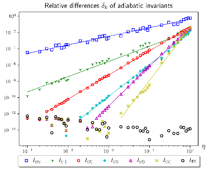
Figure 3: Numerical analysis (color online). Relative changes of the six first adiabatic invariants — and of an Ermakov-Lewis invariant IELI_{\text{EL}} — between the initial and final states, as functions of the parameter η\eta, for the harmonic oscillator with a slowly varying frequency ω⁡(η​t)=2η​t\omega(\eta t)=2^{\eta t}. The conjugate pairs (q,q˙)(q,\dot{q}) and (ρ,ρ˙)(\rho,\dot{\rho}) are integrated using the fourth-order symplectic Runge-Kutta-Nyström algorithm developed by Calvo and Sanz-Serna [24], with q⁡(0)=ρ⁡(0)=1q(0)=\rho(0)=1 and q˙​(0)=ρ˙​(0)=0\dot{q}(0)=\dot{\rho}(0)=0 as initial conditions (tt-time step: 0.0010.001). Before becoming numerically noisy when too small, δk\delta_{k} is approximately proportional to a power ηνk\eta^{\nu_{k}} with ν0=1.06±0.03\nu_{0}=1.06\pm 0.03, ν1=1.87±0.07\nu_{1}=1.87\pm 0.07, ν2=2.96±0.01\nu_{2}=2.96\pm 0.01, ν3=3.92±0.04\nu_{3}=3.92\pm 0.04, ν4=4.83±0.03\nu_{4}=4.83\pm 0.03 and ν5=6.57±0.15\nu_{5}=6.57\pm 0.15.

We now consider a frequency profile ω⁡(s)=eγ​s\omega(s)=\mathrm{e}^{\gamma s}, where γ\gamma is a constant. The recursion scheme (24yad) reveals that the τk\tau_{k}s have a certain form

τk=bk​γ2​kω2​k+1\tau_{k}=\frac{b_{k}\gamma^{2k}}{\omega^{2k+1}}

in which the bkb_{k}s are coefficients (b0=1b_{0}=1). Applying the relations (24yaf), the bkb_{k}s are again the elements of a diverging hypergeometric sequence here given by

bk=(−1)k8k​[(2​k−1)!!]3k!.b_{k}=\frac{(-1)^{k}}{8^{k}}\frac{\big[(2k-1)!!\big]^{3}}{k!}\,.

The components of the adiabatic expansion (24yae) are thus

I2​k\displaystyle I_{2k} =τk2​[q˙2−2​k+12​k−1​ω2​q2],\displaystyle=\frac{\tau_{k}}{2}\bigg[\dot{q}^{2}-\frac{2k+1}{2k-1}\,\omega^{2}q^{2}\bigg],
I2​k+1\displaystyle I_{2k+1} =τk2​(2​k+1)​γ​q​q˙.\displaystyle=\frac{\tau_{k}}{2}(2k+1)\gamma q\dot{q}.

Let us end this example by a numerical experiment in the case of a doubling of the frequency realized exponentially, i.e. for ω⁡(s)=2s=eγ​s\omega(s)=2^{s}=\mathrm{e}^{\gamma s} with γ=log⁡(2)\gamma=\log(2). For a set of values of η\eta, the equation of motion is integrated with q⁡(0)=1q(0)=1 and q˙​(0)=0\dot{q}(0)=0 as initial conditions. Then, the final values of the six first adiabatic invariants I(0),…,I(5)I_{(0)},\dots,I_{(5)} are compared with their initial values through the relative differences

δk=|I(k)​(s=1)−I(k)​(s=0)I(k)​(s=0)|.\delta_{k}=\left|\frac{I_{(k)}(s=1)-I_{(k)}(s=0)}{I_{(k)}(s=0)}\right|.

We find that δk\delta_{k} follows in good approximation a power law δk∝ηνk\delta_{k}\propto\eta^{\nu_{k}} with νk\nu_{k} close enough to k+1k+1 (see figure 3). This illustrates the fact that I(k)I_{(k)} is an adiabatic invariant of an order close to k+1k+1.

6 Final remarks

In our approach of the adiabatic invariance from Noether’s theory, we did not apply an averaging procedure on the Rund-Trautman identity, over a well-chosen slow variable [25]. Also, unlike the works of Neuenschwander et al on the subject, we did not assume a certain type of potential admitting an exact Noether symmetry and a convenient Rund-Trautman function to work on [5, 26]. Let us add that the frequency of the harmonic oscillator was supposed differentiable a certain number of times. However, in general, a time-dependent frequency is used as a transition between two regimes and discontinuities in the derivatives must be taken into account at the junctions. The great interest of the historic adiabatic invariant I0I_{0} lies in its insensitivity to them.

Appendix A Some proofs of Section 2

A.1 Transformation of an evolution for |ε||\varepsilon| small enough

The function u:t↦τ⁡(t,q⁡(t))u\colon t\mapsto\tau(t,q(t)) is smooth by assumption. Its derivative u˙\dot{u} is thus bounded on [t1,t2][t_{1},t_{2}]. Let α\alpha be an upper bound of |u˙||\dot{u}| on this interval. For an arbitrary value ε\varepsilon of the parameter such that |ε|<α−1|\varepsilon|<\alpha^{-1}, one has

OPENd​tε​(t,q⁡(t)))d​t=dd​t​[t+ε​τ​(t,q⁡(t))]=1+ε​u˙​(t)>1−|ε​u˙​(t)|>0\frac{{\mathrm{d}}t_{\varepsilon}(t,q(t)))}{{\mathrm{d}}t}=\frac{{\mathrm{d}}}{{\mathrm{d}}t}\bigg[t+\varepsilon\tau(t,q(t))\bigg]=1+\varepsilon\dot{u}(t)>1-|\varepsilon\dot{u}(t)|>0

for any time t∈[t1,t2]t\in[t_{1},t_{2}]. Since tεt_{\varepsilon} strictly increases with tt on this interval, the transformed curve of 𝒞\mathcal{C} is also the graph of an evolution.

A.2 The transformation of the velocities under Φ\Phi

Inserting (3) in (4), one has, to the first order in ε\varepsilon:

q˙εi​(tε)\displaystyle\dot{q}^{i}_{\varepsilon}(t_{\varepsilon}) =dd​t​[qi​(t)+ε​ξi​(t,q⁡(t))]/dd​t​[t+ε​τ​(t,q⁡(t))]\displaystyle=\frac{{\mathrm{d}}}{{\mathrm{d}}t}\bigg[q^{i}(t)+\varepsilon\,\xi^{i}(t,q(t))\bigg]\Bigg/\penalty\frac{{\mathrm{d}}}{{\mathrm{d}}t}\bigg[t+\varepsilon\,\tau(t,q(t))\bigg]
=[q˙i​(t)+ε​d​ξi​(t,q⁡(t))d​t]/[1+ε​d​τ​(t,q⁡(t))d​t]\displaystyle=\Bigg[\dot{q}^{i}(t)+\varepsilon\,\frac{{\mathrm{d}}\xi^{i}(t,q(t))}{{\mathrm{d}}t}\Bigg]\Bigg/\penalty\Bigg[1+\varepsilon\,\frac{{\mathrm{d}}\tau(t,q(t))}{{\mathrm{d}}t}\Bigg]
=[q˙i​(t)+ε​d​ξi​(t,q⁡(t))d​t]⋅[1−ε​d​τ​(t,q⁡(t))d​t]\displaystyle=\Bigg[\dot{q}^{i}(t)+\varepsilon\,\frac{{\mathrm{d}}\xi^{i}(t,q(t))}{{\mathrm{d}}t}\Bigg]\cdot\Bigg[1-\varepsilon\,\frac{{\mathrm{d}}\tau(t,q(t))}{{\mathrm{d}}t}\Bigg]
=q˙i​(t)+ε⁡[d​ξi​(t,q⁡(t))d​t−q˙i​(t)​d​τ​(t,q⁡(t))d​t].\displaystyle=\dot{q}^{i}(t)+\varepsilon\,\Bigg[\frac{{\mathrm{d}}\xi^{i}(t,q(t))}{{\mathrm{d}}t}-\dot{q}^{i}(t)\,\frac{{\mathrm{d}}\tau(t,q(t))}{{\mathrm{d}}t}\Bigg].

This is Formula (5).

Appendix B Some proofs of Section 3

B.1 The variation δ​S​(𝒞){\delta S(\mathcal{C})} of the action under Φ\Phi

Seeing tεt_{\varepsilon}, qε​(tε)q_{\varepsilon}(t_{\varepsilon}) and q˙ε​(tε)\dot{q}_{\varepsilon}(t_{\varepsilon}) as functions of tt through the equalities (3) and (5), one first makes the change of variable of integration [t1​ε,t2​ε]∋tε→t∈[t1,t2][t_{1\varepsilon},t_{2\varepsilon}]\ni t_{\varepsilon}\to t\in[t_{1},t_{2}] in (8):

S⁡(𝒞ε)=∫t1​εt2​εL⁡[qε​(tε)]​d​tε=∫t1t2L⁡[qε​(tε)]​d​tεd​t​𝑑t.S(\mathcal{C}_{\varepsilon})=\int_{t_{1\varepsilon}}^{t_{2\varepsilon}}L[q_{\varepsilon}(t_{\varepsilon})]\,{\mathrm{d}}t_{\varepsilon}=\int_{t_{1}}^{t_{2}}L[q_{\varepsilon}(t_{\varepsilon})]\,\frac{{\mathrm{d}}t_{\varepsilon}}{{\mathrm{d}}t}\,{\mathrm{d}}t.

Then, to the first order in ε\varepsilon, one has

S⁡(𝒞ε)\displaystyle S(\mathcal{C}_{\varepsilon}) =∫t1t2(L⁡[q⁡(t)]+ε​𝖷[1]​(L)​[q⁡(t)])​(1+ε​d​τ​(t,q⁡(t))d​t)​𝑑t\displaystyle=\int_{t_{1}}^{t_{2}}\Bigg(L[q(t)]+\varepsilon\mathsf{X}^{[1]}(L)[q(t)]\Bigg)\Bigg(1+\varepsilon\,\frac{{\mathrm{d}}\tau(t,q(t))}{{\mathrm{d}}t}\Bigg)\,{\mathrm{d}}t
=∫t1t2(L⁡[q⁡(t)]+ε​𝖷[1]​(L)​[q⁡(t)]+ε​L​[q⁡(t)]​d​τ​(t,q⁡(t))d​t)​𝑑t.\displaystyle=\int_{t_{1}}^{t_{2}}\Bigg(L[q(t)]+\varepsilon\mathsf{X}^{[1]}(L)[q(t)]+\varepsilon L[q(t)]\,\frac{{\mathrm{d}}\tau(t,q(t))}{{\mathrm{d}}t}\Bigg)\,{\mathrm{d}}t.

The first term of the integrand disappears when one forms the difference S⁡(𝒞ε)−S⁡(𝒞)S(\mathcal{C}_{\varepsilon})-S(\mathcal{C}) and Formula (9) is thus obtained.

B.2 The rearrangement (12) of the Rund-Trautman function

Using the expression (6) of the first prolongation of 𝖷\mathsf{X}, one has

𝖷[1]​(L)\displaystyle\mathsf{X}^{[1]}(L) =τ​∂L∂t+ξi​∂L∂qi+(ξ˙i−q˙i​τ˙)​∂L∂q˙i\displaystyle=\tau\,\frac{\partial L}{\partial t}+\xi^{i}\,\frac{\partial L}{\partial q^{i}}+\big(\dot{\xi}^{i}-\dot{q}^{i}\dot{\tau}\big)\frac{\partial L}{\partial\dot{q}^{i}}
=τ​∂L∂t+(ξi−q˙i​τ+q˙i​τ)​∂L∂qi+(ξ˙−q˙i​τ˙−q¨i​τ+q¨i​τ)​∂L∂q˙i\displaystyle=\tau\,\frac{\partial L}{\partial t}+\big(\xi^{i}-\dot{q}^{i}\tau+\dot{q}^{i}\tau\big)\,\frac{\partial L}{\partial q^{i}}+\big(\dot{\xi}-\dot{q}^{i}\dot{\tau}-\ddot{q}^{i}\tau+\ddot{q}^{i}\tau\big)\frac{\partial L}{\partial\dot{q}^{i}}
=τ⁡[∂L∂t+q˙i​∂L∂qi+q¨i​∂L∂q˙i]+(ξi−q˙i​τ)​∂L∂qi+(ξ˙i−q˙i​τ˙−q¨i​τ)​∂L∂q˙i\displaystyle=\tau\Bigg[\frac{\partial L}{\partial t}+\dot{q}^{i}\,\frac{\partial L}{\partial q^{i}}+\ddot{q}^{i}\,\frac{\partial L}{\partial\dot{q}^{i}}\Bigg]+\big(\xi^{i}-\dot{q}^{i}\tau\big)\,\frac{\partial L}{\partial q^{i}}+\big(\dot{\xi}^{i}-\dot{q}^{i}\dot{\tau}-\ddot{q}^{i}\tau\big)\frac{\partial L}{\partial\dot{q}^{i}}
=τ​L˙+(ξi−q˙i​τ)​∂L∂qi+dd​t​(ξi−q˙i​τ)​∂L∂q˙i\displaystyle=\tau\dot{L}+\big(\xi^{i}-\dot{q}^{i}\tau\big)\,\frac{\partial L}{\partial q^{i}}+\frac{{\mathrm{d}}}{{\mathrm{d}}t}\big(\xi^{i}-\dot{q}^{i}\tau\big)\frac{\partial L}{\partial\dot{q}^{i}}
=τ​L˙+(ξi−q˙i​τ)​∂L∂qi+dd​t​[(ξi−q˙i​τ)​∂L∂q˙i]−(ξi−q˙i​τ)​dd​t​[∂L∂q˙i]\displaystyle=\tau\dot{L}+\big(\xi^{i}-\dot{q}^{i}\tau\big)\,\frac{\partial L}{\partial q^{i}}+\frac{{\mathrm{d}}}{{\mathrm{d}}t}\Bigg[\big(\xi^{i}-\dot{q}^{i}\tau\big)\frac{\partial L}{\partial\dot{q}^{i}}\Bigg]-\big(\xi^{i}-\dot{q}^{i}\tau\big)\frac{{\mathrm{d}}}{{\mathrm{d}}t}\Bigg[\frac{\partial L}{\partial\dot{q}^{i}}\Bigg]
=τ​L˙+(ξi−q˙i​τ)​𝖤i​(L)+dd​t​[(ξi−q˙i​τ)​∂L∂q˙i],\displaystyle=\tau\dot{L}+\big(\xi^{i}-\dot{q}^{i}\tau\big)\mathsf{E}_{i}(L)+\frac{{\mathrm{d}}}{{\mathrm{d}}t}\Bigg[\big(\xi^{i}-\dot{q}^{i}\tau\big)\frac{\partial L}{\partial\dot{q}^{i}}\Bigg],

where use has been made of the Euler-Lagrange operators (7). Hence, the Rund-Trautman function (11) becomes

R=B˙−𝖷[1]​(L)−τ˙​L=I˙−(ξi−q˙i​τ)​𝖤i​(L),\displaystyle R=\dot{B}-\mathsf{X}^{[1]}(L)-\dot{\tau}L=\dot{I}-\big(\xi^{i}-\dot{q}^{i}\tau\big)\mathsf{E}_{i}(L),

with

I=B−τ​L−(ξi−q˙i​τ)​∂L∂q˙i=B+τ⁡[q˙i​∂L∂q˙i−L]−ξi​∂L∂q˙i,I=B-\tau L-\big(\xi^{i}-\dot{q}^{i}\tau\big)\frac{\partial L}{\partial\dot{q}^{i}}=B+\tau\Bigg[\dot{q}^{i}\,\frac{\partial L}{\partial\dot{q}^{i}}-L\Bigg]-\xi^{i}\,\frac{\partial L}{\partial\dot{q}^{i}}\,,

and Formulas (12) and (13) are obtained.

B.3 The gauge transformation of δ​S​(𝒞)\delta S(\mathcal{C})

Starting from

S~​(𝒞)=S⁡(𝒞)+[G⁡(t,q⁡(t))]t1t2andS~​(𝒞ε)=S⁡(𝒞ε)+[G⁡(tε,qε​(tε))]t1​εt2​ε\widetilde{S}(\mathcal{C})=S(\mathcal{C})+\Big[G(t,q(t))\Big]_{t_{1}}^{t_{2}}\quad\;\;\text{and}\quad\;\;\widetilde{S}(\mathcal{C}_{\varepsilon})=S(\mathcal{C}_{\varepsilon})+\Big[G(t_{\varepsilon},q_{\varepsilon}(t_{\varepsilon}))\Big]_{t_{1\varepsilon}}^{t_{2\varepsilon}}

one has

δ​S~​(𝒞)\displaystyle\delta\widetilde{S}(\mathcal{C}) =(S⁡(𝒞ε)+[G⁡(tε,qε​(tε))]t1​εt2​ε)−(S⁡(𝒞)+[G⁡(t,q⁡(t))]t1t2)\displaystyle=\Bigg(S(\mathcal{C}_{\varepsilon})+\Big[G(t_{\varepsilon},q_{\varepsilon}(t_{\varepsilon}))\Big]_{t_{1\varepsilon}}^{t_{2\varepsilon}}\Bigg)-\Bigg(S(\mathcal{C})+\Big[G(t,q(t))\Big]_{t_{1}}^{t_{2}}\Bigg)
=(S⁡(𝒞ε)−S⁡(𝒞))+([G⁡(tε,qε​(tε))]t1​εt2​ε−[G⁡(t,q⁡(t))]t1t2).\displaystyle=\Big(S(\mathcal{C}_{\varepsilon})-S(\mathcal{C})\Big)+\Bigg(\Big[G(t_{\varepsilon},q_{\varepsilon}(t_{\varepsilon}))\Big]_{t_{1\varepsilon}}^{t_{2\varepsilon}}-\Big[G(t,q(t))\Big]_{t_{1}}^{t_{2}}\Bigg).

The first difference is δ​S​(𝒞)\delta S(\mathcal{C}) while the second is equal to

(G⁡(t2​ε,qε​(t2​ε))−G⁡(t1​ε,qε​(t1​ε)))−(G⁡(t2,q⁡(t2))−G⁡(t1,q⁡(t1))),\Big(G(t_{2\varepsilon},q_{\varepsilon}(t_{2\varepsilon}))-G(t_{1\varepsilon},q_{\varepsilon}(t_{1\varepsilon}))\Big)-\Big(G(t_{2},q(t_{2}))-G(t_{1},q(t_{1}))\Big),

that is, to

(G⁡(t2​ε,qε​(t2​ε))−G⁡(t2,q⁡(t2)))−(G⁡(t1​ε,qε​(t1​ε))−G⁡(t1,q⁡(t1))).\Big(G(t_{2\varepsilon},q_{\varepsilon}(t_{2\varepsilon}))-G(t_{2},q(t_{2}))\Big)-\Big(G(t_{1\varepsilon},q_{\varepsilon}(t_{1\varepsilon}))-G(t_{1},q(t_{1}))\Big).

To the first order in ε\varepsilon, the last expression is thus equal to

ε​𝖷​(G)​(t2,q⁡(t2))−ε​𝖷​(G)​(t1,q⁡(t1))=ε​[𝖷⁡(G)​(t,q⁡(t))]t1t2.\varepsilon\mathsf{X}(G)(t_{2},q(t_{2}))-\varepsilon\mathsf{X}(G)(t_{1},q(t_{1}))=\varepsilon\Big[\mathsf{X}(G)(t,q(t))\Big]_{t_{1}}^{t_{2}}\,.

One deduces Formula (14).

Appendix C Some proofs of Section 4

C.1 The change of variable (t,q)→(T,Q)(t,q)\to(T,Q)

Locally, along the integral curves of Φ\Phi parametrized by ε\varepsilon, the coordinates tt and qq varies according to

d​td​ε=τ⁡(t)andd​qd​ε=ξ⁡(t,q)=12​τ˙​(t)​q+ψ⁡(t).\frac{{\mathrm{d}}t}{{\mathrm{d}}\varepsilon}=\tau(t)\qquad\text{and}\qquad\frac{{\mathrm{d}}q}{{\mathrm{d}}\varepsilon}=\xi(t,q)=\frac{1}{2}\,\dot{\tau}(t)q+\psi(t). (24yag)

One seeks a new time TT and a new coordinate QQ varying as

d​Td​ε=1andd​Qd​ε=0.\frac{{\mathrm{d}}T}{{\mathrm{d}}\varepsilon}=1\qquad\text{and}\qquad\frac{{\mathrm{d}}Q}{{\mathrm{d}}\varepsilon}=0. (24yah)

Dividing the first equality of (24yah) by the first equality of (24yag), one has

d​Td​t=1τ⁡(t).\frac{{\mathrm{d}}T}{{\mathrm{d}}t}=\frac{1}{\tau(t)}\,.

This equation is automatically verified if TT is defined as a function of tt alone by

T=∫td​t′τ⁡(t′).T=\int^{t}\frac{{\mathrm{d}}t^{\prime}}{\tau(t^{\prime})}\,.

Then, dividing the second equality of (24yag) by the first, one obtains the linear differential equation

d​qd​t=τ˙​(t)2​τ​(t)​q+ψ⁡(t)τ⁡(t).\frac{{\mathrm{d}}q}{{\mathrm{d}}t}=\frac{\dot{\tau}(t)}{2\tau(t)}\,q+\frac{\psi(t)}{\tau(t)}\,.

It is easily integrated with the usual methods to give the relation between qq and tt along the integral curves of Φ\Phi:

q=τ⁡(t)​(∫tψ⁡(t′)τ​(t′)3/2​d​t′+C)q=\sqrt{\tau(t)}\Bigg(\int^{t}\frac{\psi(t^{\prime})}{\tau(t^{\prime})^{3/2}}\,{\mathrm{d}}t^{\prime}+C\Bigg)

where CC is a constant. Hence, the integral curves are solved as Q=CQ=C, with

Q=qτ​(t)−∫tψ⁡(t′)τ​(t′)3/2​d​t′Q=\frac{q}{\sqrt{\tau}(t)}-\int^{t}\frac{\psi(t^{\prime})}{\tau(t^{\prime})^{3/2}}\,{\mathrm{d}}t^{\prime}

which thus verifies the second equality of (24yah). The change of variables (t,q)→(T,Q)(t,q)\to(T,Q) is licit since TT strictly increases with tt for any evolution and since TT and QQ are independent:

∂(T,Q)∂(t,q)=|∂tT∂qT∂tQ∂qQ|=1τ​(t)3/2≠0.\frac{\partial(T,Q)}{\partial(t,q)}=\left|\begin{array}[]{cc}\partial_{t}T&\partial_{q}T\\ \partial_{t}Q&\partial_{q}Q\end{array}\right|=\frac{1}{\tau(t)^{3/2}}\neq 0.

Finally, one can easily check that 𝖷⁡(T)=1\mathsf{X}(T)=1 and 𝖷⁡(Q)=0\mathsf{X}(Q)=0, i.e. that 𝖷=∂T\mathsf{X}=\partial_{T}.

C.2 The form (18) of the potential VV

Multiplying the expression of R0R_{0} in (15) by τ\tau yields

τ​R0=τ​∂tB+𝖷⁡(τ​V).\tau R_{0}=\tau\partial_{t}B+\mathsf{X}(\tau V). (24yai)

Then, using the form of BB in (16), taking its partial derivative with respect to tt, and expressing the result as a function of tt and QQ through

q=τ​(Q+α)withα⁡(t)=∫tψτ3/2​𝑑t,q=\sqrt{\tau}\big(Q+\alpha\big)\quad\text{with}\quad\alpha(t)=\int^{t}\frac{\psi}{\tau^{3/2}}\,{\mathrm{d}}t,

one obtains

∂tB=14​𝜏…q2+ψ¨​q+χ˙=k2​(t)​Q2+k1​(t)​Q+k0​(t),\partial_{t}B=\frac{1}{4}\,{\mathop{\kern 0.0pt\tau}\limits^{\vbox to-1.4pt{\kern-2.0pt\hbox{...}\vss}}}q^{2}+\ddot{\psi}q+\dot{\chi}=k_{2}(t)\,Q^{2}+k_{1}(t)\,Q+k_{0}(t), (24yaj)

with

k2​(t)=14​𝜏…τ,k1​(t)=ψ¨​τ+12​α​𝜏…τ,k0​(t)=α​ψ¨​τ+14​α2​𝜏…τ+χ˙.k_{2}(t)=\frac{1}{4}\,{\mathop{\kern 0.0pt\tau}\limits^{\vbox to-1.4pt{\kern-2.0pt\hbox{...}\vss}}}\tau\;\,,\quad k_{1}(t)=\ddot{\psi}\sqrt{\tau}+\frac{1}{2}\,\alpha{\mathop{\kern 0.0pt\tau}\limits^{\vbox to-1.4pt{\kern-2.0pt\hbox{...}\vss}}}\tau\;\,,\quad k_{0}(t)=\alpha\ddot{\psi}\sqrt{\tau}+\frac{1}{4}\,\alpha^{2}{\mathop{\kern 0.0pt\tau}\limits^{\vbox to-1.4pt{\kern-2.0pt\hbox{...}\vss}}}\tau+\dot{\chi}.

One remarks that the variable ρ⁡(t)=τ\rho(t)=\sqrt{\tau} is such that

12​𝜏…τ=dd​t​(ρ3​ρ¨).\frac{1}{2}\,{\mathop{\kern 0.0pt\tau}\limits^{\vbox to-1.4pt{\kern-2.0pt\hbox{...}\vss}}}\tau=\frac{{\mathrm{d}}}{{\mathrm{d}}t}\Big(\rho^{3}\ddot{\rho}\Big). (24yak)

Hence

k2​(t)=d​K2​(t)d​twithK2​(t)=12​ρ3​ρ¨.k_{2}(t)=\frac{{\mathrm{d}}K_{2}(t)}{{\mathrm{d}}t}\quad\text{with}\quad K_{2}(t)=\frac{1}{2}\,\rho^{3}\ddot{\rho}.

Applying two times the Leibniz rule on the product ψ​ρ\psi\rho and using the fact that ψ=τ3/2​α˙=ρ3​α˙\psi=\tau^{3/2}\dot{\alpha}=\rho^{3}\dot{\alpha}, one obtains

ψ¨​τ=ψ¨​ρ=dd​t​(ψ˙​ρ−ψ​ρ˙)+ψ​ρ¨=dd​t​[ρ2​d⁡(ρ2​α˙)d​t]+α˙​ρ3​ρ¨\ddot{\psi}\sqrt{\tau}=\ddot{\psi}\rho=\frac{{\mathrm{d}}}{{\mathrm{d}}t}\Big(\dot{\psi}\rho-\psi\dot{\rho}\Big)+\psi\ddot{\rho}=\frac{{\mathrm{d}}}{{\mathrm{d}}t}\Bigg[\rho^{2}\,\frac{{\mathrm{d}}(\rho^{2}\dot{\alpha})}{{\mathrm{d}}t}\Bigg]+\dot{\alpha}\rho^{3}\ddot{\rho} (24yal)

and thus

k1​(t)=dd​t​[ρ2​d⁡(ρ2​α˙)d​t]+α˙​ρ3​ρ¨+α​dd​t​(ρ3​ρ¨),k_{1}(t)=\frac{{\mathrm{d}}}{{\mathrm{d}}t}\Bigg[\rho^{2}\,\frac{{\mathrm{d}}(\rho^{2}\dot{\alpha})}{{\mathrm{d}}t}\Bigg]+\dot{\alpha}\rho^{3}\ddot{\rho}+\alpha\,\frac{{\mathrm{d}}}{{\mathrm{d}}t}\Big(\rho^{3}\ddot{\rho}\Big),

that is,

k1​(t)=d​K1​(t)d​twithK1​(t)=ρ2​(ρ2​α¨+2​ρ​ρ˙​α˙+ρ​ρ¨​α).k_{1}(t)=\frac{{\mathrm{d}}K_{1}(t)}{{\mathrm{d}}t}\quad\text{with}\quad K_{1}(t)=\rho^{2}\Big(\rho^{2}\ddot{\alpha}+2\rho\dot{\rho}\dot{\alpha}+\rho\ddot{\rho}\alpha\Big).

Then, using (24yak) and (24yal), one has

k0​(t)\displaystyle k_{0}(t) =α​dd​t​[ρ2​d⁡(ρ2​α˙)d​t]+α​α˙​ρ3​ρ¨+12​α2​dd​t​(ρ3​ρ¨)+χ˙\displaystyle=\alpha\,\frac{{\mathrm{d}}}{{\mathrm{d}}t}\Bigg[\rho^{2}\,\frac{{\mathrm{d}}(\rho^{2}\dot{\alpha})}{{\mathrm{d}}t}\Bigg]+\alpha\dot{\alpha}\rho^{3}\ddot{\rho}+\frac{1}{2}\,\alpha^{2}\,\frac{{\mathrm{d}}}{{\mathrm{d}}t}\Big(\rho^{3}\ddot{\rho}\Big)+\dot{\chi}
=dd​t​[α​ρ2​d⁡(ρ2​α˙)d​t]−α˙​ρ2​d⁡(ρ2​α˙)d​t+12​d⁡(α2)d​t​ρ3​ρ¨+12​α2​dd​t​(ρ3​ρ¨)+χ˙.\displaystyle=\frac{{\mathrm{d}}}{{\mathrm{d}}t}\Bigg[\alpha\rho^{2}\,\frac{{\mathrm{d}}(\rho^{2}\dot{\alpha})}{{\mathrm{d}}t}\Bigg]-\dot{\alpha}\rho^{2}\,\frac{{\mathrm{d}}(\rho^{2}\dot{\alpha})}{{\mathrm{d}}t}+\frac{1}{2}\frac{{\mathrm{d}}(\alpha^{2})}{{\mathrm{d}}t}\,\rho^{3}\ddot{\rho}+\frac{1}{2}\,\alpha^{2}\,\frac{{\mathrm{d}}}{{\mathrm{d}}t}\Big(\rho^{3}\ddot{\rho}\Big)+\dot{\chi}.

The second term is clearly the tt-derivative of −(ρ2α˙)2/2-(\rho^{2}\dot{\alpha})^{2}/2 while the sum of the two next terms is the tt-derivative of α2​ρ3​ρ¨/2\alpha^{2}\rho^{3}\ddot{\rho}/2. Hence, one has

k0​(t)=d​K0​(t)d​twithK0​(t)=ρ2​(ρ2​α​α¨+2​ρ​ρ˙​α​α˙+12​ρ​ρ¨​α2−β)k_{0}(t)=\frac{{\mathrm{d}}K_{0}(t)}{{\mathrm{d}}t}\quad\text{with}\quad K_{0}(t)=\rho^{2}\bigg(\rho^{2}\alpha\ddot{\alpha}+2\rho\dot{\rho}\alpha\dot{\alpha}+\frac{1}{2}\,\rho\ddot{\rho}\alpha^{2}-\beta\bigg)

where was introduced the quantity

β⁡(t)=ψ22​τ2−χτ=12​ρ2​α˙2−χρ2.\beta(t)=\frac{\psi^{2}}{2\tau^{2}}-\frac{\chi}{\tau}=\frac{1}{2}\,\rho^{2}\dot{\alpha}^{2}-\frac{\chi}{\rho^{2}}\,.

Consequently, the multiplication of (24yaj) by τ\tau gives

τ​∂tB\displaystyle\tau\partial_{t}B =τ​d​K2d​t​Q2+τ​d​K1d​t​Q+τ​d​K0d​t=d​K2d​T​Q2+d​K1d​T​Q+d​K0d​T\displaystyle=\tau\,\frac{{\mathrm{d}}K_{2}}{{\mathrm{d}}t}\,Q^{2}+\tau\,\frac{{\mathrm{d}}K_{1}}{{\mathrm{d}}t}\,Q+\tau\,\frac{{\mathrm{d}}K_{0}}{{\mathrm{d}}t}=\frac{{\mathrm{d}}K_{2}}{{\mathrm{d}}T}\,Q^{2}+\frac{{\mathrm{d}}K_{1}}{{\mathrm{d}}T}\,Q+\frac{{\mathrm{d}}K_{0}}{{\mathrm{d}}T}
=∂∂T​(K2​Q2+K1​Q+K0)Q\displaystyle=\frac{\partial}{\partial T}\Big(K_{2}Q^{2}+K_{1}Q+K_{0}\Big)_{Q}

and Equation (24yai) becomes

ρ2​R0=∂∂T​(K2​Q2+K1​Q+K0+ρ2​V)\rho^{2}R_{0}=\frac{\partial}{\partial T}\Big(K_{2}Q^{2}+K_{1}Q+K_{0}+\rho^{2}V\Big) (24yam)

since 𝖷=∂T\mathsf{X}=\partial_{T} in the adapted system. Therefore, taking an integral with respect to TT (with QQ kept constant), there is a function W⁡(Q)W(Q) such that

∫Tρ2​R0​𝑑T=K2​Q2+K1​Q+K0+ρ2​V−W⁡(Q).\int^{T}\hskip-5.69054pt\rho^{2}R_{0}\,{\mathrm{d}}T=K_{2}Q^{2}+K_{1}Q+K_{0}+\rho^{2}V-W(Q). (24yan)

It still remains to isolate VV and reexpress QQ in terms of the old coordinates to obtain Formula (18).

C.3 The gauge term (20)

We seek a solution GG to the gauge condition B+𝖷⁡(G)=0B+\mathsf{X}(G)=0 with

B=14​τ¨​q2+ψ˙​q+χ.B=\frac{1}{4}\,\ddot{\tau}q^{2}+\dot{\psi}q+\chi.

Expressing qq as a function of tt and QQ, one has

B=τ⁡(ℓ2​(t)​Q2+ℓ1​(t)​Q+ℓ0​(t)),B=\tau\Big(\ell_{2}(t)Q^{2}+\ell_{1}(t)Q+\ell_{0}(t)\Big), (24yao)

with

ℓ2​(t)=14​τ¨,ℓ1​(t)=12​α​τ¨+ψ˙τ,ℓ0​(t)=14​α2​τ¨+α​ψ˙τ+χτ.\ell_{2}(t)=\frac{1}{4}\,\ddot{\tau}\quad,\quad\ell_{1}(t)=\frac{1}{2}\,\alpha\ddot{\tau}+\frac{\dot{\psi}}{\sqrt{\tau}}\quad,\quad\ell_{0}(t)=\frac{1}{4}\,\alpha^{2}\ddot{\tau}+\alpha\,\frac{\dot{\psi}}{\sqrt{\tau}}+\frac{\chi}{\tau}\,.

One has obviously

ℓ2​(t)=d​L2​(t)d​twithL2​(t)=14​τ˙=12​ρ​ρ˙.\ell_{2}(t)=\frac{{\mathrm{d}}L_{2}(t)}{{\mathrm{d}}t}\quad\text{with}\quad L_{2}(t)=\frac{1}{4}\,\dot{\tau}=\frac{1}{2}\,\rho\dot{\rho}.

Then, using the Leibniz rule as above, one has

ℓ1​(t)=dd​t​(12​α​τ˙)−12​α˙​τ˙+ψ˙τ=dd​t​(12​α​τ˙)−ψ​τ˙2​τ3/2+ψ˙τ,\ell_{1}(t)=\frac{{\mathrm{d}}}{{\mathrm{d}}t}\Bigg(\frac{1}{2}\,\alpha\dot{\tau}\bigg)-\frac{1}{2}\,\dot{\alpha}\dot{\tau}+\frac{\dot{\psi}}{\sqrt{\tau}}=\frac{{\mathrm{d}}}{{\mathrm{d}}t}\Bigg(\frac{1}{2}\,\alpha\dot{\tau}\bigg)-\frac{\psi\dot{\tau}}{2\tau^{3/2}}+\frac{\dot{\psi}}{\sqrt{\tau}}\,,

that is,

ℓ1​(t)=d​L1​(t)d​twithL1​(t)=12​α​τ˙+ψτ=α​ρ​ρ˙+α˙​ρ2.\ell_{1}(t)=\frac{{\mathrm{d}}L_{1}(t)}{{\mathrm{d}}t}\quad\text{with}\quad L_{1}(t)=\frac{1}{2}\,\alpha\dot{\tau}+\frac{\psi}{\sqrt{\tau}}=\alpha\rho\dot{\rho}+\dot{\alpha}\rho^{2}.

As for ℓ0​(t)\ell_{0}(t), one has

ℓ0​(t)\displaystyle\ell_{0}(t) =dd​t​(14​α2​τ˙)−12​α˙​α​τ˙+α​ψ˙τ+χτ\displaystyle=\frac{{\mathrm{d}}}{{\mathrm{d}}t}\Bigg(\frac{1}{4}\,\alpha^{2}\dot{\tau}\Bigg)-\frac{1}{2}\,\dot{\alpha}\alpha\dot{\tau}+\alpha\,\frac{\dot{\psi}}{\sqrt{\tau}}+\frac{\chi}{\tau}
=dd​t​(14​α2​τ˙)+α⁡(−ψ​τ˙2​τ3/2+ψ˙τ)+χτ\displaystyle=\frac{{\mathrm{d}}}{{\mathrm{d}}t}\Bigg(\frac{1}{4}\,\alpha^{2}\dot{\tau}\Bigg)+\alpha\Bigg(-\frac{\psi\dot{\tau}}{2\tau^{3/2}}+\frac{\dot{\psi}}{\sqrt{\tau}}\Bigg)+\frac{\chi}{\tau}
=dd​t​(14​α2​τ˙)+α​dd​t​(ψτ)+χτ\displaystyle=\frac{{\mathrm{d}}}{{\mathrm{d}}t}\Bigg(\frac{1}{4}\,\alpha^{2}\dot{\tau}\Bigg)+\alpha\,\frac{{\mathrm{d}}}{{\mathrm{d}}t}\Bigg(\frac{\psi}{\sqrt{\tau}}\Bigg)+\frac{\chi}{\tau}
=dd​t​(14​α2​τ˙+α​ψτ)−α˙​ψτ+χτ\displaystyle=\frac{{\mathrm{d}}}{{\mathrm{d}}t}\Bigg(\frac{1}{4}\,\alpha^{2}\dot{\tau}+\alpha\,\frac{\psi}{\sqrt{\tau}}\Bigg)-\dot{\alpha}\,\frac{\psi}{\sqrt{\tau}}+\frac{\chi}{\tau}
=dd​t​(12​ρ​ρ˙​α2+ρ2​α​α˙)−12​ρ2​α˙2−β,\displaystyle=\frac{{\mathrm{d}}}{{\mathrm{d}}t}\Bigg(\frac{1}{2}\,\rho\dot{\rho}\alpha^{2}+\rho^{2}\alpha\dot{\alpha}\Bigg)-\frac{1}{2}\,\rho^{2}\dot{\alpha}^{2}-\beta,

that is,

ℓ0​(t)=d​L0​(t)d​twithL0​(t)=12​ρ​ρ˙​α2+ρ2​α​α˙−∫t(12​ρ2​α˙2+β)​𝑑t.\displaystyle\ell_{0}(t)=\frac{{\mathrm{d}}L_{0}(t)}{{\mathrm{d}}t}\quad\text{with}\quad L_{0}(t)=\frac{1}{2}\,\rho\dot{\rho}\alpha^{2}+\rho^{2}\alpha\dot{\alpha}-\int^{t}\Bigg(\frac{1}{2}\,\rho^{2}\dot{\alpha}^{2}+\beta\Bigg){\mathrm{d}}t.

Therefore,

B\displaystyle B =τ​d​L2d​t​Q2+τ​d​L1d​t​Q+τ​d​L0d​t=d​L2d​T​Q2+d​L1d​T​Q+d​L0d​t\displaystyle=\tau\,\frac{{\mathrm{d}}L_{2}}{{\mathrm{d}}t}\,Q^{2}+\tau\,\frac{{\mathrm{d}}L_{1}}{{\mathrm{d}}t}\,Q+\tau\,\frac{{\mathrm{d}}L_{0}}{{\mathrm{d}}t}=\frac{{\mathrm{d}}L_{2}}{{\mathrm{d}}T}\,Q^{2}+\frac{{\mathrm{d}}L_{1}}{{\mathrm{d}}T}\,Q+\frac{{\mathrm{d}}L_{0}}{{\mathrm{d}}t}
=∂∂T​(L2​Q2+L1​Q+L0)Q,\displaystyle=\frac{\partial}{\partial T}\Big(L_{2}Q^{2}+L_{1}Q+L_{0}\Big)_{Q},

and the gauge condition B+𝖷⁡(G)=0B+\mathsf{X}(G)=0 reduces to

∂∂T​(L2​Q2+L1​Q+L0+G)Q=0.\frac{\partial}{\partial T}\Big(L_{2}Q^{2}+L_{1}Q+L_{0}+G\Big)_{Q}=0.

It suffices to choose

G=−L2​Q2−L1​Q−L0.G=-L_{2}Q^{2}-L_{1}Q-L_{0}\,. (24yap)

Replacing QQ with its expression as a function of tt and qq, one obtains Formula (20).

C.4 The adapted Lagrangian (21)

The adapted Lagrangian L¯\overline{L} is such that L¯​d​T=L​d​t+d​G\overline{L}{\mathrm{d}}T=L{\mathrm{d}}t+{\mathrm{d}}G, i.e.

L¯=L​d​td​τ+d​Gd​T=L​ρ2+∂G∂T+Q̊​∂G∂Q=ρ2​(12​q˙2−V)−B+Q̊​∂G∂Q\overline{L}=L\,\frac{{\mathrm{d}}t}{{\mathrm{d}}\tau}+\frac{{\mathrm{d}}G}{{\mathrm{d}}T}=L\,\rho^{2}+\frac{\partial G}{\partial T}+\mathring{Q}\,\frac{\partial G}{\partial Q}=\rho^{2}\Bigg(\frac{1}{2}\,\dot{q}^{2}-V\Bigg)-B+\mathring{Q}\,\frac{\partial G}{\partial Q}

where the empty bullet symbolizes the total TT-derivative. Then, using

q˙=d​qd​t=dd​t​[ρ⁡(Q+α)]=ρ​Q˙+ρ˙​Q+d⁡(ρ​α)d​t=Q̊ρ+ρ˙​Q+(ρ˙​α+ρ​α˙)\dot{q}=\frac{{\mathrm{d}}q}{{\mathrm{d}}t}=\frac{{\mathrm{d}}}{{\mathrm{d}}t}\Big[\rho(Q+\alpha)\Big]=\rho\,\dot{Q}+\dot{\rho}Q+\frac{{\mathrm{d}}(\rho\alpha)}{{\mathrm{d}}t}=\frac{\mathring{Q}}{\rho}+\dot{\rho}Q+(\dot{\rho}\alpha+\rho\dot{\alpha})

together with the expressions (24yan), (24yao) and (24yap) of VV, BB and GG respectively, one obtains

L¯=\displaystyle\overline{L}= 12​Q̊2+M4​(t)​Q̊​Q+M3​(t)​Q̊+M2​(t)​Q2+M1​(t)​Q+M0​(t)\displaystyle\frac{1}{2}\,\mathring{Q}^{2}+M_{4}(t)\mathring{Q}Q+M_{3}(t)\mathring{Q}+M_{2}(t)Q^{2}+M_{1}(t)Q+M_{0}(t)
−W⁡(Q)−∫Tρ2​R0​𝑑T\displaystyle-W(Q)-\int^{T}\hskip-5.69054pt\rho^{2}R_{0}\,{\mathrm{d}}T

with

M4​(t)=ρ​ρ˙−2​L2,M1​(t)=ρ2​ρ˙​(ρ˙​α+ρ​α˙)+K1−ρ2​ℓ1,M3​(t)=ρ⁡(ρ˙​α+ρ​α˙)−L1,M0​(t)=12​ρ2​(ρ˙​α+ρ​α˙)2+K0−ρ2​ℓ0.M2​(t)=12​ρ2​ρ˙2+K2−ρ2​ℓ2,\begin{array}[]{ll}M_{4}(t)=\rho\dot{\rho}-2L_{2}\,,&M_{1}(t)=\rho^{2}\dot{\rho}(\dot{\rho}\alpha+\rho\dot{\alpha})+K_{1}-\rho^{2}\ell_{1}\,,\\ M_{3}(t)=\rho(\dot{\rho}\alpha+\rho\dot{\alpha})-L_{1}\,,&M_{0}(t)=\displaystyle\frac{1}{2}\,\rho^{2}(\dot{\rho}\alpha+\rho\dot{\alpha})^{2}+K_{0}-\rho^{2}\ell_{0}\,.\\ M_{2}(t)=\displaystyle\frac{1}{2}\,\rho^{2}\dot{\rho}^{2}+K_{2}-\rho^{2}\ell_{2}\,,\end{array}

But one verifies with the definitions of the various quantities introduced in C.2 and C.3 that the Mi​(t)M_{i}(t)s identically vanish. The adapted Lagrangian (21) is thus obtained.

References

  • [1] Noether E 1918 Gött. Nachr. 2 235 in German ; the first English translation is due to Tavel M A [Transport Theor. Stat. 1, 186 (1971)] and a more recent one can be found in [3]
  • [2] Bessel-Hagen E 1921 Math. Ann. 84 258 in German ; English translation : Albinius M and Ibramigov M H in Archives of ALGA 3, 33 (2006)
  • [3] Kosmann-Schwarzbach Y 2011 The Noether theorems, Invariance and conservation laws in the twentieth century (New York: Springer)
  • [4] Logan J D 1977 Invariant Variational Principles (New York: Academic Press)
  • [5] Neuenschwander D E 2017 Emmy Noether’s wonderful theorem 2nd ed (Baltimore: The John Hopkins University Press)
  • [6] Rund H 1972 Util. Math. 2 205
  • [7] Trautman A 1967 Commun. Math. Phys. 6 248
  • [8] Lutzky M 1978 J. Phys. A: Math. Gen. 11 249
  • [9] Prince G E and Eliezer C J 1980 J. Phys. A: Math. Gen. 13 815
  • [10] Leone R and Gourieux T 2015 Eur. J. Phys. 36 065022
  • [11] Lochak P and Meunier C 1988 Multiphase Averaging for Classical Systems – With Applications to Adiabatic Theorems (New York: Springer)
  • [12] Lewis H R and Leach P G L 1982 J. Math. Phys. 23 2371
  • [13] Ehrenfest P 1917 KNAW, Proceedings vol 19 (Amsterdam) p 576
  • [14] Kulsrud R M 1957 Phys. Rev. 106 205
  • [15] Olver P J 1993 Applications of Lie Groups to Differential Equations 2nd ed (New York: Springer)
  • [16] Lamé G 1859 Leçons sur les coordonnées curvilignes et leurs diverses applications (Paris: Mallet-Bachellier) in French
  • [17] Spivak M 1999 A Comprehensive Introduction to Differential Geometry 3rd ed vol 1 (Houston: Publish or Perish)
  • [18] Goldstein H, Poole C and Safko J 2001 Classicle Mechanics 3rd ed (San Fransisco: Addison Wesley)
  • [19] Leone R and Haas F 2017 Eur. J. Phys. 38 045005
  • [20] Ermakov V P 1880 Univ. Izv. Kiev 9 1
  • [21] Lewis H R 1967 Phys. Rev. Lett. 18 510
  • [22] Fock V A 1928 Z. Phys. 49 323 in German; English translation in L. D. Faddeev, L. A. Khalfin and I. V. Komarov (Eds.), V. A. Fock – Selected Works: Quantum Mechanics and Quantum Field Theory (Chapman & Hall/CRC, New York, 2004).
  • [23] Arnold V I 1989 Mathematical Methods in Classical Mechanics 2nd ed (New York: Springer)
  • [24] Calvo M P and Sanz-Serna J M 1993 SIAM J. Sci. Comput. 14 936
  • [25] Boccaletti D and Pucacco G 1999 Theory of orbits. Volume 2: Perturbative and Geometrical Methods (Berlin: Springer)
  • [26] Neuenschwander D E and Starkey S R 1993 Am. J. Phys. 61 1008