Physical deep learning based on optimal control of dynamical systems Preprint: APS/123-QED
Abstract
Deep learning is the backbone of artificial intelligence technologies, and it can be regarded as a kind of multilayer feedforward neural network. An essence of deep learning is information propagation through layers. This suggests that there is a connection between deep neural networks and dynamical systems in the sense that information propagation is explicitly modeled by the time-evolution of dynamical systems. In this study, we perform pattern recognition based on the optimal control of continuous-time dynamical systems, which is suitable for physical hardware implementation. The learning is based on the adjoint method to optimally control dynamical systems, and the deep (virtual) network structures based on the time evolution of the systems are used for processing input information. As a key example, we apply the dynamics-based recognition approach to an optoelectronic delay system and demonstrate that the use of the delay system allows for image recognition and nonlinear classifications using only a few control signals. This is in contrast to conventional multilayer neural networks, which require a large number of weight parameters to be trained. The proposed approach provides insight into the mechanisms of deep network processing in the framework of an optimal control problem and presents a pathway for realizing physical computing hardware.
I Introduction
The recent rapid progress of information technologies, including machine learning, has led to studies on novel computing concepts and hardware, such as neuromorphic processing Markovic2020; Rabinovich2006; Furber2016; Merolla2014; Feldmann2019; Tait2017, reservoir computing Versraeten2007; Jaeger2004; Tanaka2019; Appeltant2011; Brunner2013; Inubushi2020, and deep learning LeCun2015; Xu2018; Lin2018; Shen2017. In particular, deep learning has become a groundbreaking tool for data processing owing to its high-level performance LeCun2015. Furthermore, the energy-efficient computing for deep learning is gaining importance with the rising need for processing large amounts of data XChen2014.
An underlying key factor of deep learning is its high expressive power, which is the result of the layer-to-layer propagation of information in the deep network. This expressive power enables the representation of extremely complex functions in a manner that cannot be achieved using shallow networks with the same number of neurons Poole2016; Montufar2014. Interestingly, recent studies have reported that the information propagation in multilayer systems can be expressed as the time evolution of dynamical systems Liu2019; Chen2018; Benning2019; Haber2017. From the point of view of dynamical systems, the learning process of networks can be regarded as the optimal control of the dynamical systems Liu2019; Chen2018. This viewpoint suggests that there is a connection between deep neural networks and dynamical systems and indicates the possibility of using dynamical systems as physical deep-learning machines.
In this paper, we reveal the potential of dynamical systems with optimal control for the physical implementation. We propose a deep neural network-like architecture using dynamical systems with delayed feedback and show that delayed feedback allows for the virtual construction of a deep network structure in a physically single node using a time-division multiplexing method. In the proposed approach, the virtual deep network for information propagation comes from the time evolution of delay systems; the systems are optimally controlled such that information processing, including classification, is facilitated. The significant difference between our deep network and ordinary deep neural network architectures is that the learning via optimal control is realized by only a few control signals and minimal weight parameters, whereas the learning by conventional deep neural networks requires a large number of weight parameters Shen2017; Lin2018. The proposed approach using optimal control is applicable for a wide variety of experimentally controllable systems; it allows for simple but large-scale deep networks in physical systems with a few control parameters.
II Multilayer neural networks and dynamical systems
First, we briefly discuss the relationship between multilayer neural networks and dynamical systems. Let a dataset to be learned be composed of inputs, and their corresponding target vectors, , where . and are dimensions of the inputs and target vectors, respectively. The goal of supervised learning is to find a function that maps inputs onto corresponding targets, . To this end, we consider an output function, , parameterized by the -dimensional vector, , and the following loss function:
| (1) |
where is a function of the distance between the target and the output, . is determined such that loss function is minimized, i.e., output corresponds to target .
It is well-known that a neural network model with an appropriate activation function is a good candidate for representing function owing to its universal approximation capability Cybenko1989; Funahashi1989; Sonoda2017. In multilayer neural networks, the output, , is given by the layer-to-layer propagation of an input, [Fig. 1(a)]. The layer-to-layer propagation based on multilayer network structures plays a crucial role in increasing expressivity Poole2016 and enhancing learning performance. In this study, instead of standard multilayer networks, we utilize information propagation in a continuous-time dynamical system,
| (2) |
where is the state vector at time and represents a control signal vector. Based on the correspondence between a multilayer network [Fig. 1(a)] and a dynamical system [Fig. 1(b)], we suppose that an input is set as an initial state . Additionally, the corresponding output, , is given by the time evolution (feedforward propagation) of the state vector, , up to the end time , i.e., , where is a parameter matrix determined in the training process. Loss function is obtained by repeating the aforementioned feedforward propagation for all training data instances and using their outputs. The goal of the learning is to find an optimal control vector, , and a parameter vector, , such that is minimized, i.e., . It should be noted that learning using a discretized version of Eq. (2) directly corresponds to that using a residual network (ResNet) Chen2018; Benning2019.
One strategy for finding optimal controls and parameters is to compute the gradients of the loss function, i.e., the direction of the steepest descent, and to update control and parameter vectors in an iterative manner, i.e, and , respectively. In a simple gradient descent method, and are chosen such that the largest local decrease of is obtained. is simply selected in the opposite direction of the gradient , e.g., , where is the learning rate, which is usually a small positive number. is obtained using the adjoint method developed in the context of optimal control problems Kirk2004; Sage1977 as follows:
| (3) |
where is a small positive number, and . is the adjoint state vector that satisfies the end condition at , . For , the time evolution of is given by
| (4) |
The derivation of Eqs. (3) and
(4) is shown in Appendix A.
We note that integrating Eq. (4) in the backward direction (from to
) corresponds to backpropagation in neural networks.
In summary, the algorithm for computing optimal and is
as follows:
(i) Set the input, , for the th data instance as
an initial state, i.e., .
(ii) Forward propagation:
Starting from initial state , integrate Eq. (2)
and obtain the end state, .
Then, compute the output, .
(iii) Repeat the forward propagation for all data instances
and compute loss function .
(iv) Backpropagation: Integrate adjoint Eq. (4)
for in the backward direction from
with .
(v) Compute
and using Eq. (3) with
appropriate learning rates, and .
(vi) Update control signal and parameter .
For the updates, one can use different optimization algorithms
Ruder2016.

II.1 Binary classification problem
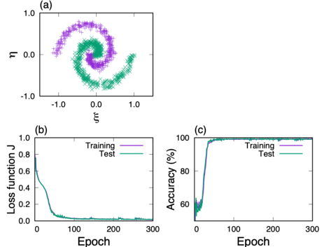
Here, we use an abstract dynamical system for solving a typical fundamental problem, the binary classification problem. The goal of the binary classification is to classify a given dataset into two categories labeled as, for example, “0” or “1”. For this, we here consider a simple dynamical model, , where the state vector is two-dimensional, . Weight and bias are used as control signals. We apply this model to the binary classification problem for a spiral dataset, , where is distributed around one of two spirals in the -plane, as shown in Fig. 2(a), and is labeled by as “0” or “1” according to the classes. For the classification, we used one-hot encoding, i.e., target corresponding to input was set as if and if . For the output, , the softmax function was used: , where , , and . If , approaches , whereas if , approaches . was selected as a cross-entropy loss function, . A training set of data points was used to train and . The classification accuracy was evaluated using a test set of data points. For the gradient-based optimization, we used the Adam optimizer Kingma2014 with a batch size of .
Figures 2(b) and 2(c) show the learning curve and classification accuracy for the training and test datasets, respectively. The loss function monotonically decreases, and the classification accuracy approaches 100 . For sufficient training over 300 training epochs, the classification accuracy was over 99 when end time is set as , where is the time step used in the simulation. Figure 3 shows the time evolution of the two distributions constituting the spiral dataset. During the evolution, the distributions of the initial states are disentangled [Figs. 3(a-d)] and become linearly separable at end time [Fig. 3(d)] to aid the classification at the softmax output layer. As a result, any input state can be classified into either of two classes [Fig. 3(e)]. We note that the classification based on disentanglement is different from that of other schemes utilizing dynamical systems, e.g., reservoir computing, whose classification is based on the mapping of input information onto a high-dimensional feature space Tanaka2019. In addition, we note that the disentanglement is facilitated as end time increases, i.e., the number of layers increases, and high classification accuracy is achieved for , as shown in Fig. 3(f). A slight decrease in classification accuracy at is attributed to slowdown of the training due to a local plateau of loss function , which is occasionally caused in a non-convex optimization problem Dauphin2014. At , we confirmed that a classification accuracy of over 99 was obtained when the number of training epochs is extended to 400.

III Physical implementation in delay systems
In the previous section, we showed binary classification based on optimal control in a two-dimensional dynamical model, where weight and bias were used as control signals. The excellent performance of this demonstration suggests the realization of deep learning in various physical systems, such as coupled oscillators, fluids, and elastic bodies. However, for processing high-dimensional data, a number of signals must be used to control the high-dimensional degrees of freedom in the systems; this may be difficult in terms of physical implementation in an actual system.
To overcome the difficulty, we propose the use of delay systems to achieve feasible optimal control of numerous degrees of freedom with limited control signals. It is known that delay systems can be regarded as infinite-dimensional dynamical systems, as visualized in a time–space representation Arecchi1992. Furthermore, delay systems can support numerous virtual neurons using a time-division multiplexing method Appeltant2011. In addition, they can exhibit various dynamical phenomena, including stable motion, periodic motion, and high dimensional chaos, with experimentally controllable parameters, e.g., delay time and feedback strength Uchida; Soriano2013. Thus, their high expressivity as well as controllability are promising.
III.1 Learning by optimal control in a delay system
We introduce a training method based on the optimal control of a delay system, the time evolution of which is governed by the following equation:
| (5) |
where and represent the state vector and control signal vector at time , respectively, and is the delay time. The aforementioned equation can be integrated by setting for as an initial condition.
The information dynamics can intuitively be interpreted by a space–time representation Arecchi1992 based on the time discretization of Eq. (5), , where , , , , and . In this representation, can be regarded as the th network node in the th layer, which is affected by an adjacent node, , and node in the th layer, as shown in Fig. 4.
Feedforward propagation is carried out as follows: First, an input, , is encoded as for in the initial condition. Then, Eq. (5) is numerically solved to obtain in the th layer (corresponding to in continuous time). The output, , is computed using the nodes in the th layer, , as shown in Fig. 4. In the continuous time representation, the output is defined as , where . and are the weight and bias parameters to be trained, respectively, and is the state vector starting from the initial state . Finally, loss function [Eq. (1)] is computed.
To minimize loss function , a gradient-based optimization is used, where , , are updated in an iterative manner. In a gradient descent method, the update variations, , , and , can be chosen as follows:
| (6) |
| (7) |
The details of these derivations are provided in Appendix B. In the aforementioned equations, , is a function of , and for is the learning rate which is a small positive number. In Eq. (6), is the adjoint state vector, which satisfies . can be obtained by solving the following adjoint equations in the backward direction,
| (8) |
for , and
| (9) |
for .

III.2 Optoelectronic delay system
As an effective and feasible example, we consider the use of an optoelectronic delay system, as shown in Fig. 5. The delay system is composed of a laser, optoelectronic intensity modulator, photodetector, and electrical filter to construct a time-delay feedback loop. The time evolution of the system state, , is given by the following equations Murphy2010:
| (10) |
| (11) |
where is the normalized voltage, and and are the time constants of the low-pass and high-pass filters, respectively. represents the feedback strength. and are electronic signals added to the feedback loop, which are used as control signals in the system.

III.3 Results
III.3.1 Binary classification
We demonstrate binary classification for a spiral dataset, as shown in Fig. 2(a), with the aforementioned optoelectronic delay system. The goal of binary classification is to classify two categories labeled as “0” or “1” for the spiral dataset, . In the same manner as that described in Sec. II.1, target is set as if , whereas if . Output is set as the softmax function, i.e., , where , and . Then, is defined as the cross-entropy loss function, . In this simulation, the following parameters settings were applied: ms, s, and s. The input, , is encoded as the initial state of , i.e., for and for . We set and as the initial control signals and and () as the initial weight and bias parameters. We used the Adam optimizer Kingma2014 with a batch size of for the gradient-based optimization. The update equations for , , , and are shown in Appendix C.
In the aforementioned conditions, the classification accuracy at training epoch 100 was 99.1 when the feedback strength was and the end time was . To gain insight into the classification mechanism, we investigated the effect of the control signals, and , and weights, , , on the delay dynamics. Figures 6(a–e) show the trained control signals, and , weights, and , and four instances of at training epoch 100. in a range of is used for computing the (softmax) outputs, , which represents the probability that the input is classified as class . Considering that is a function of , we computed . corresponds to the correlation between (softmax) weights used for the classification as class and the th instance, , which starts from the initial states labeled as . Figures 6(f) and 6(g) show the histograms of the correlation values, , for 500 instances. The correlation values are positive for in most cases, whereas they are negative for . In other words, in most cases. Thus, the softmax output for classification as is activated by starting from the initial states with the same class . These results reveal that the trained control signals control each trajectory such that it is positively correlated to the weight and is maximized.
Figure 7 shows the classification accuracy at training epoch 100 as a function of feedback strength and end time . As seen in this figure, classification performance is low for . In this regime, the system exhibits transient behavior to stable limit cycle motion, which is insensitive to external perturbations [Figs. 8(a) and 8(b)]. This means that it is difficult to control the system. When increases (), the system starts to exhibit complex behavior and becomes sensitive to the control signals for a large end time, , as shown in Figs. 8(c) - 8(f). Sensitivity plays a role in aiding the classification. However, extremely high sensitivity makes it difficult to control the system and decreases classification performance, as observed for and in Fig. 7. Consequently, a high classification performance of over 99 is achieved with moderate values of and , suggesting that the transient behavior around the edge of chaos plays a crucial role in classification.


III.3.2 MNIST handwritten digit classification
To investigate the classification performance for a higher dimensional dataset, we use the MNIST handwritten digit dataset, commonly used as a standard benchmark for learning MNIST; LeCun1998. The dataset has a training set of 60,000 2828 pixel grayscale images of ten handwritten digits, along with a test set of 10,000 images.
To set an initial state of the system state, an input image of pixels is enlarged to double its length and width; it is transformed to a -dimensional vector, where . The vector components are sequentially set as at time with a time interval of s. The input process is repeated -times to encode the information of the input image as for all . The training of the delay system is based on the gradient-based optimization using the Adam optimizer with a batch size of 100. The maximum number of epochs to train was set as 50 to ensure the convergence of the training process. As a demonstration of the classifications at epoch 50, we show four examples of the softmax outputs, which represents the probability that the input image belongs to one of the 10-classes, in Figs. 9(a)–(d).
Figures 9(e) and 9(f) show the classification accuracy for various values of feedback strength and delay time , where is fixed. For this image dataset, the delay system with exhibits relatively high classification performance. The best classification accuracy for this system is 97 . We emphasize that accurate classification is achieved with two training signals, , and minimal weight parameters, , and , , owing to the time-division multiplexing encoding method based on the delay structure, as discussed in Sec. III.1. This is in contrast to conventional neural networks, where more than hundreds or thousands of weight parameters need to be trained.
We can see that classification accuracy improves as delay time increases [Fig.9(f)]. As discussed in Sec. III.1, the effective number of the network nodes, , depends on in the delay system, i.e., . This suggests that larger-scale networks, i.e., systems with a longer delay, play an important role in achieving better classification for this large dataset.

IV Conclusion
We discussed the applicability of optimally-controlled dynamical systems to information processing. The dynamics-based processing provides insight into the mechanism of information processing based on deep network structures, and it can be easily implemented in physical systems. As a particular example, we introduced an optoelectronic delay system. The delay system can be trained to perform nonlinear classification and image recognition with only a few control signals and classification weights based on the time-division multiplexing method. This feature of delay systems is an advantage to hardware implementation of the systems and is distinctively different from conventional neural networks, which require a large number of training parameters. The dynamics-based processing based on optimal control can be applied to various physical systems to construct not only feedforward networks but also recurrent neural networks, including reservoir computing. This provides a novel direction for physics-based computing.
Acknowledgements.
This work was supported, in part, by JSPS KAKENHI (Grant No. 20H042655) and JST PRESTO (Grant No. JPMJPR19M4). The authors thank Profs. Kazutaka Kanno and Atsushi Uchida for valuable discussions on optoelectronic delay systems.Appendix A Adjoint method for Eq. (2)
We derive the adjoint equations used to find an optimal control vector . The first step is to incorporate the constraint of Eq. (2), , into loss function with the Lagrangian multiplier (adjoint) vector as follows:
| (12) |
where is the state vector starting from the initial state, , and . Considering that the second term of Eq. (12) is rewritten as
| (13) |
we can obtain
| (14) |
Let and be the variations of and loss function in terms of the variation , respectively. Then, variation is computed as follows:
| (15) |
where , and is used in the aforementioned derivation because the initial state is fixed as . As the Lagrangian multiplier, , can be set freely, we select such that it satisfies the following equation:
| (16) | ||||
| (17) |
In this case, we obtain a simple form of as follows: . Accordingly, when the variation is set as
| (18) |
with a positive constant , is satisfied. Thus, monotonically decreases when is updated as .
Appendix B Adjoint method for Eq. (5)
We consider the update variations, , , and , for the optimization of the delay system that obeys Eq. (5). In the same manner as that shown in Appendix A, we consider the augmented loss function incorporating Eq. (5) as follows:
| (19) |
where , , and is the Lagrangian multiplier (adjoint vector).
Variation in terms of the variation is expressed as
| (20) |
where . In the aforementioned equation, considering , variation is rewritten as
| (21) |
When is selected such that and the following equations are satisfied,
| (22) |
for , and
| (23) |
for , we can obtain a simple form of , as When is selected as
| (24) |
is always satisfied.
Then, we consider variations and in terms of the variations of weights and bias parameters, respectively. In the same manner shown earlier, we obtain, in terms of the weight variation and in terms of the weight variation . Clearly, when and are set as follows:
| (25) |
and
| (26) |
with small positive constants, and , and .
Appendix C Update equations for , , , and in the optoelectronic delay system
In this study, we set the loss function as , where , and . In this case, the adjoint equations for are given as follows for ,
| (27) | ||||
| (28) |
and for ,
| (29) | ||||
| (30) |
where , , , , and . Then, the update variables of control signal vectors are given as follows:
| (31) | ||||
| (32) |
and the update variables of weights and bias parameters are
| (33) | ||||
| (34) |
References
- (1) D. Markovi, A. Mizrahi, D. Querlioz, and J. Grollier, Physics for neuromorphic computing, Nature Reviews Physics 2, 499 (2020).
- (2) M. I. Rabinovich, P. Varona, A. I. Selverston, and H. D. I. Abarbanel, Dynamical principles in neuroscience, Rev. Mod. Phys. 78, 1213 (2006).
- (3) S. Furber, Large-scale neuromorphic computing systems, J. Neural Eng. 13, 051001 (2016).
- (4) P. A. Merolla, J. V. Arthur, R. Alvarez-Icaza, A. S. Cassidy, J. Sawada, F. Akopyan, B. L. Jackson, N. Imam, C. Guo, Y. Nakamura et al., A million spiking-neuron integrated circuit with a scalable communication network and interface, Science 345, 668 (2014).
- (5) J. Feldmann, N. Youngblood, C.D. Wright, H. Bhaskaran, and W. H. P. Pernice, All-optical spiking neurosynaptic networks with self-learning capabilities, Nature 569, 208 (2019).
- (6) A. N. Tait, T. Ferreira de Lima, E. Zhou, A. X. Wu, M. A. Nahmias, B. J. Shastri, and P. R. Prucnal, Neuromorphic photonic networks using silicon photonic weight banks, Sci. Rep. 7, 7430 (2017).
- (7) D. Verstraeten, B. Schrauwen, M. D’Haene, D. Stroobandt, An experimental unification of reservoir computing methods, Neural. Netw. 20, 391 (2007).
- (8) H. Jaeger, and H. Haas, Harnessing nonlinearity: predicting chaotic systems and saving energy in wireless communication, Science 304, 78 (2004).
- (9) G. Tanaka, T. Yamane, J. B. Héroux, R. Nakane, N. Kanazawa, S. Takeda, H. Numata, D. Nakano, and A. Hirose, Recent Advances in Physical Reservoir Computing: A Review, Neural Networks 115, 100-123 (2019).
- (10) L. Appeltant, M. C. Soriano, G. Van der Sande, J. Danckaert, S. Massar, J. Dambre, B. Schrauwen, C. R. Mirasso, and I. Fischer, Information processing using a single dynamical node as complex system, Nat. Commun. 2, 468 (2011).
- (11) D. Brunner, M. C. Soriano, C. R. Mirasso, and I. Fischer, Parallel photonic information processing at gigabyte per second data rates using transient states, Nat. Commun. 4, 1364 (2013).
- (12) M. Inubushi, and S. Goto, Transfer learning for nonlinear dynamics and its application to fluid turbulence, Phys. Rev. E 105, 043301 (2020).
- (13) Y. LeCun, Y. Bengio, and G. Hinton, Deep learning, Nature 521, 436 (2015).
- (14) X. Xu, Y. Ding, S. X. Hu, M. Niemier, J. Cong, Y. Hu, and Y. Shi, Scaling for edge inference of deep neural networks, Nat. Electron. 1, 216 (2018).
- (15) X. Lin, Y. Rivenson, N. T. Yardimci, M. Veli, Y. Luo, M. Jarrahi, and A. Ozcan, All-optical machine learning using diffractive deep neural networks, Science 361(6406) 1004-1008 (2018).
- (16) Y. Shen, N. C. Harris, S. Skirlo, M. Prabhu, T. Baehr-Jones, M. Hochberg, X. Sun, S. Zhao, H. Larochelle, D. Englund, and M. Soljačić, Deep learning with coherent nanophotonic circuits, Nat. Photonics 11, 441-446 (2017).
- (17) X. Chen and X. Lin, Big Data Deep Learning: Challenges and Perspectives, IEEE Access, 2, 514 (2014).
- (18) B. Poole, S. Lahiri, M. Raghu, J. Sohl-Dickstein, and S. Ganguli, Exponential expressivity in deep neural networks through transient chaos, Adv. Neural. Inf. Process Syst. 29, 3360-3368 (2016).
- (19) F Montufar, R. Pascanu, K. Cho, and Y. Bengio, On the number of linear regions of deep neural networks, Adv. Neural Inf. Process. Syst. 27, 2924 (2014).
- (20) G.-H. Liu and E. A. Theodorou, Deep Learning Theory Review: An Optimal Control and Dynamical Systems Perspective, arXiv:1908.10920v2 (2019).
- (21) T. Q. Chen, Y. Rubanova, J. Bettencourt, and D. K. Duvenaud, Neural ordinary differential equations, Adv. Neural. Inf. Process. Syst., 31, 6572-6583 (2018).
- (22) M. Benning, E. Celledoni, M. J Ehrhardt, B. Owren, and C.-B. Schönlieb, Deep learning as optimal control problems: models and numerical methods, arXiv:1904.05657 (2019).
- (23) E. Haber and L. Ruthotto, Stable architectures for deep neural networks, Inverse Problems, 34 014004 (2017).
- (24) G. Cybenko, Approximation by superpositions of a sigmoidal function, Math. Control Signal Systems 2, 303 (1989).
- (25) K. Funahashi, On the approximate realization of continuous mappings by neural networks, Neural Networks, 2 183 (1989).
- (26) S. Sonoda, and N. Murata, Neural network with unbounded activation functions is universal approximator, Appl. Comput. Harm. Anal., 43 233 (2017).
- (27) D. E. Kirk, Optimal Control Theory: An Introduction, (Dover Publications, Inc., Mineola, NY, 2004)
- (28) A. P. Sage, Optimum Systems Control, (Prentice-Hall, 1977).
- (29) S. Ruder, An overview of gradient descent optimization algorithms, arXiv:1609.04747.
- (30) D. P. Kingma and J. Ba, Adam: A Method for Stochastic Optimization, International Conference on Learning Representations (2015); arXiv:1412.6980.
- (31) Y. Dauphin, R. Pascanu, C. Gulcehre, K. Cho, S. Ganguli, and Y. Bengio, Identifying and attacking the saddle point problem in high-dimensional non-convex optimization, Advances in Neural Information Processing Systems, 27 2933–2941 (2014).
- (32) F. T. Arecchi, G. Giacomelli, A. Lapucci, and R. Meucci, Two-dimensional representation of a delayed dynamical system, Phys. Rev. A, 45 R4225z(R) (1992).
- (33) A. Uchida, Optical Communication with Chaotic Lasers (Wiley-VCH, 2012).
- (34) M. C. Soriano , J. Garcia-Ojalvo, C. R. Mirasso, and I. Fischer, Complex photonic: Dynamics and applications of delay-coupled semiconductor lasers, Rev. Mod. Phys. 85, 421 (2013).
- (35) T. E. Murphy, A. B. Cohen, B. Ravoori, K. R. B. Schmitt, A. V. Setty, F. Sorrentino, C. R. S. Williams, E. Ott and R. Roy, Complex dynamics and synchronization of delayed-feedback nonlinear oscillators, Phil. Trans. R. Soc. A. 368, 343 (2010).
- (36) Y. LeCun, C. Cortes, and C. J. C. Burges, The MNIST database of handwritten digits, http://yann.lecun.com/exdb/mnist
- (37) Y. LeCun, L. Bottou, Y. Bengio, and P. Haffner, Gradient-based learning applied to document recognition, Proceedings of the IEEE, 86, 2278 (1998).