Graph Neural Networks: Taxonomy, Advances and TrendsDOI: 0000Journal: TISTVolume: 0000000CCS: Computing methodologies Neural networksCCS: Computing methodologies Learning latent representations

The spectral graph convolution operator is defined via the graph Fourier transform. For two graph signals $x$ and $y$ on $G$, their spectral graph convolution $x\ast_{G}y$ is defined by

where $\circledast$ denotes the element-wise Hadamard product (Joan Bruna et al. 2014; Federico Monti et al. 2017a; Mikael Henaff et al. 2015). The spectral graph convolution can be rewritten as

where $f_{\theta}$ is a diagonal matrix consisting of the learnable parameters. That is, the signal $x$ is filtered by the spectral graph filter (or graph convolution kernel) $f_{\theta}$. For a $d^{(l)}\text{-dimensional}$ graph signal $X^{(l)}$ on $G$, the output $X^{(l+1)}$ yielded by a graph convolution layer, namely $d^{(l+1)}\text{-dimensional}$ graph signal on $G$, can be written as

where $f_{\theta,j,k}^{(l)}$ is a spectral graph filter, i.e. a $N\times N$ diagonal matrix consisting of learnable parameters corresponding to the $j\text{-th}$ graph signal at $l\text{-th}$ layer and the $k\text{-th}$ graph signal at $(l+1)\text{-th}$ layer. The computational framework of the spectral GCNN in Eq. (5) is demonstrated in Fig. 2. It is worth noting that the calculation of the above graph convolution layer takes $O(N^{3})$ time and $O(N^{2})$ space to perform the eigendecomposition of $\overline{L}_{G}$ especially for large graphs. The article (Vikas Verma et al. 2019) proposes a regularization technique, namely GraphMix, to augment the vanilla GCNN with a parameter-sharing Fully Connected Network (FCN).

Spectral Graph Filter. Many studies (Mikael Henaff et al. 2015) focus on designing different spectral graph filters. In order to circumvent the eigendecomposition, the spectral graph filter $f_{\theta}$ can formulated as a $K\text{-localized}$ polynomial of the eigenvalues of the normalized graph Laplacian $\overline{L}_{G}$ (Thomas N. Kipf and Max Welling 2017; Ruoyu Li et al. 2018; Michaël Defferrard et al. 2016), i.e.

In practice, the $K\text{-localized}$ Chebyshev polynomial (Michaël Defferrard et al. 2016) is a favorable choice of formulating the spectral graph filter, i.e.

where the Chebyshev polynomial is defined as

and $\widetilde{\Lambda}=\frac{2}{\lambda_{\text{max}}}\Lambda-\mathbb{I}_{N}$. The reason why $\widetilde{\Lambda}=\frac{2}{\lambda_{\text{max}}}\Lambda-\mathbb{I}_{N}$ is because it can map eigenvalues $\lambda\in\left[0,\lambda_{\text{max}}\right]$ into $[-1,1]$. This filter is $K\text{-localized}$ in the sense that it leverages information from nodes which are at most $K\text{-hops}$ away. In order to further decrease the computational cost, the $1\text{st-order}$ Chebyshev polynomial is used to define the spectral graph filter. Specifically, it lets $\lambda_{\text{max}}\approx 2$ (because the largest eigenvalue of $\overline{L}_{G}$ is less than or equal to 2 (Chung 1992)) and $\theta=\theta_{0}=-\theta_{1}$. Moreover, the renormalization trick is used here to mitigate the limitations of the vanishing/exploding gradient, namely substituting $\widetilde{D}_{G}^{-\frac{1}{2}}\widetilde{A}_{G}\widetilde{D}_{G}^{-\frac{1}{2}}$ for $\mathbb{I}_{N}+D_{G}^{-\frac{1}{2}}A_{G}D_{G}^{-\frac{1}{2}}$ where $\widetilde{A}_{G}=A_{G}+\mathbb{I}_{N}$ and $\widetilde{D}_{G}=\text{diag}\left(\sum_{k=1}^{N}\widetilde{A}[1,k],\cdots,\sum_{k=1}^{N}\widetilde{A}[N,k]\right)$. As a result, the Graph Convolutional Network (GCN) (Thomas N. Kipf and Max Welling 2017; Sami Abu-EL-Haija et al. 2019a) can be defined as

The Chebyshev spectral graph filter suffers from a drawback that the spectrum of $\overline{L}_{G}$ is linearly mapped into $\left[-1,1\right]$. This drawback makes it hard to specialize in the low frequency bands. In order to mitigate this problem, Michael M. Bronstein et al (Ron Levie et al. 2019) proposes the Cayley spectral graph filter via the $\text{order-}r$ Cayley polynomial $f_{c,h}(\lambda)=c_{0}+2\text{Re}\left(\sum_{j=0}^{r}c_{h}\mathcal{C}(\lambda)^{j}\right)$ with the Cayley transform $\mathcal{C}(\lambda)=\frac{\lambda-i}{\lambda+i}$. Moreover, there are many other spectral graph filters, e.g. (Ruoyu Li et al. 2018; Renjie Liao et al. 2019; Chenyi Zhuang and Qiang Ma 2018; Felix Wu et al. 2019; Ana {̆S}u{̆s}njara et al. 2015; Tong Zhang et al. 2018; Jian Du et al. 2018; Matthew Baron 2018; Yuzhou Chen et al. 2020; Sami Abu-EL-Haija et al. 2019b). In addition, some studies employ the capsule network (Sara Sabour et al. 2017) to construct capsule-inspired GNNs (Xinyi Zhang and Lihui Chen 2019; Saurabh Verma and Zhili Zhang 2018; Marcelo Daniel Gutierrez Mallea et al. 2019).

Overcoming Time and Memory Challenges. A chief challenge for GCNNs is that their training cost is strikingly expensive, especially on huge and sparse graphs. The reason is that the GCNNs require full expansion of neighborhoods for the feed-forward computation of each node, and large memory space for storing intermediate results and outputs. In general, two approaches, namely sampling (Wenbing Huang et al. 2018; Jie Chen et al. 2018; Jianfei Chen et al. 2018; Hongyang Gao et al. 2018) and decomposition (Weilin Chiang et al. 2019; Xin Jiang et al. 2020), can be employed to mitigate the time and memory challenges for the spectral GCNNs.

Depth Trap of Spectral GCNNs. A bottleneck of GCNNs is that their performance maybe decease with ever-increasing number of layer. This decay is often attributed to three factors: (1) overfitting resulting from the ever-increasing number of parameters; (2) gradient vanishing/explosion during training; (3) oversmoothing making vertices from different clusters more and more indistinguishable. The reason for oversmoothing is that performing the Laplacian smoothing many times forces the features of vertices within the same connected component to stuck in stationary points (Qimai Li et al. 2018). There are some available approaches, e.g. (Yawei Luo et al. 2018; Lingxiao Zhao and Leman Akoglu 2020; Yu Rong et al. 2020; Afshin Rahimi et al. 2018; Rupesh Kumar Srivastava et al. 2015), to circumvent the depth trap of the spectral GCNNs.

Original spatial GCNNs (Vincenzo Di Massa et al. 2006; Gori et al. 2005; Franco Scarselli et al. 2009; Franco Scarselli et al. 2008) constitutes a transition function, which must be a contraction map in order to ensure the uniqueness of states, and an update function. In the following, we firstly introduce a generic framework of the spatial GCNN, and then investigate its variants.

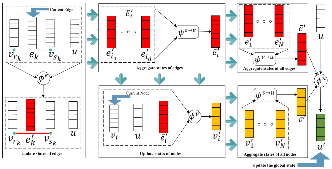
Graph networks (GNs) as generic architectures with relational inductive bias (Peter W. Battaglia et al. 2018) provide an elegant interface for learning entities, relations and structured knowledge. Specifically, GNs are composed of GN blocks in a sequential, encode-process-decode or recurrent manner. GN blocks contain three kinds of update functions, namely $\phi^{e}(\cdot),\phi^{v}(\cdot),\phi^{u}(\cdot)$, and three kinds of aggregation functions, namely $\psi^{e\rightarrow v}(\cdot),\psi^{e\rightarrow u}(\cdot),\psi^{v\rightarrow u}(\cdot)$. The iterations are described as follows.

where $e_{k}$ is an arch from $v_{s_{k}}$ to $v_{r_{k}}$, $E^{\prime}_{i}=\left\{(e^{\prime}_{k},s_{k},r_{k}):r_{k}=i,k=1,\cdots,M\right\}$, $V^{\prime}=\left\{v^{\prime}_{i}:i=1,\cdots,N\right\}$ and $E^{\prime}=\left\{(e^{\prime}_{k},s_{k},r_{k}):k=1,\cdots,M\right\}$, see Fig. 3. It is noted that the aggregation functions should be invariant to any permutations of nodes or edges. In practice, the GN framework can be used to implement a wide variety of architectures in accordance with three key design principles, namely flexible representations, configuable within-block structure and flexible multi-block architectures. Below, we introduce three prevalent variants of the GNs, namely Message Passing Neural Networks (MPNNs) (Justin Gilmer et al. 2017), Non-local Neural Networks (NLNNs) (Alvaro Sanchez-Gonzalez et al. 2018) and GraphSAGE (William L. Hamilton et al. 2017).

Variants of GNs——MPNNs. MPNNs (Justin Gilmer et al. 2017) have two phases, a message passing phase and a readout phase. The message passing phase is defined by a message function $M_{l}$ (playing the role of the composition of the update function $\psi^{e\rightarrow v}(\cdot)$ and the update function $\phi^{e}(\cdot)$) and a vertex update function $U_{l}$ (playing the role of the update function $\phi^{v}(\cdot)$). Specifically,

where $e_{v,u}$ denotes the feature vector of the edge with two endpoints $v$ and $u$. The readout phase computes a universal feature vector for the whole graph using a readout function $R(\cdot)$, i.e. $u=R\left(\left\{x_{v}^{(L)}:v\in V\right\}\right)$. The readout function $R(\cdot)$ should be invariant to permutations of nodes. A lot of GCNNs can be regarded as special forms of the MPNN, e.g. (David Duvenaud et al. 2015; Yujia Li et al. [n.d.]; Peter Battaglia et al. 2016; Steven Kearnes et al. 2016).

Variants of GNs——NLNNs. NLNNs (Alvaro Sanchez-Gonzalez et al. 2018) give a general definition of non-local operations (Antoni Buades et al. 2005) which is a flexible building block and can be easily integrated into convolutional/recurrent layers. Specifically, the generic non-local operation is defined as

where $f(\cdot,\cdot)$ denotes the affinity between $x_{s}$ and $x_{t}$, and $\mathcal{C}(x_{s})=\sum_{t}f(x_{s},x_{t})$ is a normalization factor. The affinity function $f(\cdot,\cdot)$ is of the following form

1. (1)

   Gaussian: $f(x_{s},x_{t})=e^{x_{s}^{T}x_{t}}$;

2. (2)

   Embedded Gaussian: $f(x_{s},x_{t})=e^{\theta(x_{s})^{T}\eta(x_{t})}$, where $\theta(x_{s})=W_{\theta}x_{s}$ and $\eta(x_{t})=W_{\eta}x_{t}$;

3. (3)

   Dot Product: $f(x_{s},x_{t})=\theta(x_{s})^{T}\eta(x_{t})$;

4. (4)

   Concatenation: $f(x_{s},x_{t})=\text{ReLU}(w_{f}^{T}\left[\theta(x_{s}),\eta(x_{t})\right])$.

The non-local building block is defined as $z_{s}=W_{z}y_{s}+x_{s}$ where "$+x_{s}$" denotes a residual connection. It is noted that $f(\cdot,\cdot)$ and $g(\cdot)$ play the role of $\phi^{e}(e_{k},v_{r_{k}},v_{s_{k}},u)$, and the summation in Eq. (10) plays the role of $\psi^{e\rightarrow v}(E^{\prime}_{i})$.

Variants of GNs——GraphSAGE. GraphSAGE (SAmple and aggreGatE) (William L. Hamilton et al. 2017) is a general inductive framework capitalizing on node feature information to efficiently generate node embedding vectors for previously unseen nodes. Specifically, GraphSAGE is composed of an aggregation function $\text{{Aggregate}}^{(l)}(\cdot)$ and an update function $\text{{Update}}^{(l)}$, i.e.

where $N_{G}(v)$ denotes a fixed-size set of neighbors of $v$ uniformly sampling from its whole neighbors. The aggregation function is of the following form

1. (1)

   Mean Aggregator: $x_{v}^{(l)}=\sigma\left(W\cdot\text{{Mean}}\left(\left\{x_{v}^{(l-1)}\right\}\cup\left\{x_{u}^{(l-1)}:u\in N_{G}(v)\right\}\right)\right)$;

2. (2)

   LSTM Aggregator: applying the LSTM (Sepp Hochreiter and Jürgen Schmidhuber 1997) to aggregate the neighbors of $v$;

3. (3)

   Pooling Aggregator: $\text{{Aggregate}}^{(l)}=\max\left(\left\{\sigma\left(Wx_{u}^{(l)}+b\right):u\in N_{G}(v)\right\}\right)$.

Note that the aggregation function and update function play the role of $\psi^{e\rightarrow v}(E^{\prime}_{i})$ and $\phi^{v}(v_{i},\overline{e}^{\prime}_{i},u)$ in formula (9) respectively.

Variants of GNs——Hyperbolic GCNNs. The Euclidean GCNNs aim to embed nodes in a graph into a Euclidean space. This will incur a large distortion especially when embedding real-world graphs with scale-free and hierarchical structure. Hyperbolic GCNNs pave an alternative way of embedding with little distortion. The $n\text{-dimensional}$ hyperbolic space (Caglar Gulcehre et al. 2019; Richard C. Wilson et al. 2014), denoted as $\mathbb{H}_{K}^{n}$, is a unique, complete, simply connected $d\text{-dimensional}$ Riemannian manifold with constant negative sectional curvature $-\frac{1}{K}$, i.e.

where the Minkowski inner produce $\langle x,y\rangle_{\mathcal{M}}=-x_{0}y_{0}+\sum_{j=1}^{d}x_{j}y_{j},\forall x,y\in\mathbb{R}^{n+1}$. Its tangent space centered at point $x$ is denoted as $\mathcal{T}_{x}\mathbb{H}_{K}^{n}=\left\{v\in\mathbb{R}^{n+1}:\langle x,v\rangle_{\mathcal{M}}=0\right\}$. Given $x\in\mathbb{H}_{K}^{n}$, let $u\in\mathcal{T}_{x}\mathbb{H}_{K}^{n}$ be unit-speed. The unique unit-speed geodesic $\gamma_{x\rightarrow u}(\cdot)$ such that $\gamma_{x\rightarrow u}(0)=x$ and $\dot{\gamma}_{x\rightarrow u}(0)=u$ is denoted as $\gamma_{x\rightarrow u}(t)=\cosh\left(\frac{t}{\sqrt{K}}\right)x+\sqrt{K}\sinh\left(\frac{t}{\sqrt{K}}\right),u,t>0.$ The intrinsic distance between two points $x,y\in\mathbb{H}_{K}^{n}$ is then equal to

Therefore, the above $n\text{-dimensional}$ hyperbolic space with constant negative sectional curvature $-\frac{1}{K}$ is usually denoted as $\left(\mathbb{H}_{K}^{n},d_{\mathcal{M}}^{K}(\cdot,\cdot)\right)$. In particular, $\mathbb{H}_{1}^{n}$, i.e. $K=1$, is called the hyperboloid model of the hyperbolic space. Hyperbolic Graph Convolutional Networks (HGCN) (Ines Chami et al. 2019) benefit from the expressiveness of both GCNNs and hyperbolic embedding. It employs the exponential and logarithmic maps of the hyperboloid model, respectively denoted as $\exp_{x}^{K}(\cdot)$ and $\log_{x}^{K}(\cdot)$, to realize the mutual transformation between Euclidean features and hyperbolic ones. Let $\|v\|_{\mathcal{M}}=\langle v,v\rangle_{\mathcal{M}},v\in\mathcal{T}_{x}\mathbb{H}_{K}^{n}$. The $\exp_{x}^{K}(\cdot)$ and $\log_{x}^{K}(\cdot)$ are respectively defined to be

where $x\in\mathbb{H}_{K}^{n}$, $v\in\mathcal{T}_{x}\mathbb{H}_{K}^{n}$ and $y\in\mathbb{H}_{K}^{n}$ such that $y\neq 0$ and $y\neq x$. The HGCN architecture is composed of three components: a Hyperbolic Feature Transform (HFT), an Attention-Based Aggregation (ABA) and a Non-Linear Activation with Different Curvatures (NLADC). They are respectively defined as

where $o=\left(\sqrt{K},0,\cdots,0\right)\in\mathbb{H}_{K}^{n}$, the subscript $j$ denotes the indices of nodes, the superscript $l$ denotes the layer of the HGCN. The linear transform in hyperboloid manifold is defined to be $W\otimes^{K}x^{H}=\exp_{o}^{K}\left(W\log_{o}^{K}(x^{H})\right)$ and $x^{H}\oplus^{K}b=\exp_{x^{H}}^{K}\left(P_{o\rightarrow x^{H}}^{K}(b)\right)$, where $P_{o\rightarrow x^{H}}^{K}(b)$ is the parallel transport from $\mathcal{T}_{o}\mathbb{H}_{K}^{n}$ to $\mathcal{T}_{x^{H}}\mathbb{H}_{K}^{n}$. The attention-based aggregation is defined to be $\text{{Aggregate}}^{K}(x^{H})_{j}=\exp_{x_{j}^{H}}^{K}\left(\sum_{k\in N_{G}(j)}\omega_{j,k}\log_{x_{j}^{H}}^{K}\left(x_{k}^{H}\right)\right)$, where the attention weight $\omega_{j,k}=\text{Softmax}_{k\in N_{G}(j)}\left(\text{MLP}\left(\log_{o}^{K}\left(x_{j}^{H}\right)\bowtie\log_{o}^{K}\left(x_{k}^{H}\right)\right)\right)$.

Higher-Order Spatial GCNNs. the aforementioned GCNN architectures are constructed from the microscopic perspective. They only consider nodes and edges, yet overlook the higher-order substructures and their connections, i.e subgraphs consisting of at least 3 nodes. Here, we introduce the studies on the $k\text{-dimensional}$ GCNNs (Christopher Morris et al. 2019). Specifically, they take higher-order graph structures at multiple scales into consideration by leveraging the $k\text{-Weisfeiler-Leman}$ ($k\text{-WL}$) graph isomorphism test so that the message passing is performed directly between subgraph structures rather than individual nodes. Let $\{\hskip-3.41432pt\{\cdots\}\hskip-3.41432pt\}$ denote a multiset, $\text{{Hash}}(\cdot)$ a hashing function and $C_{l,k}^{(l)}(s)$ the node coloring (label) of $s=(s_{1},\cdots,s_{k})\in V^{k}$ at the $l\text{-th}$ time. Moreover, let $N_{G}^{j}(s)=\left\{(s_{1},\cdots,s_{j-1},r,s_{j+1},\cdots,s_{k}):r\in V\right\}$. The $k\text{-WL}$ is computed by

where $c_{j}^{(l+1)}=\text{{Hash}}\left(\left\{\hskip-3.41432pt\left\{C_{l,k}^{(l)}(s^{\prime}):s^{\prime}\in N_{G}^{j}(s)\right\}\hskip-3.41432pt\right\}\right)$. The $k\text{-GCNN}$ computes new features of $s\in V^{k}$ by multiple computational layers. Each layer is computed by

In practice, the local $k\text{-GCNNs}$ is often employed to learn the hierarchical representations of nodes in order to scale to larger graphs and mitigate the overfitting problem.

Other Variants of GNs. In addition to the aforementioned GNs and its variants, there are still many other spatial GCNNs which is defined from other perspectives, e.g. Diffusion-Convolutional Neural Network (DCNN) (James Atwood and Don Towsley 2016), Position-aware Graph Neural Network (P-GNN) (Jiaxue You et al. 2019), Memory-based Graph Neural Network (MemGNN) and Graph Memory Network (GMN) (Amir H. Khasahmadi et al. 2020), Graph Partition Neural Network (GPNN) (Renjie Liao et al. 2018), Edge-Conditioned Convolution (ECC) (Martin Simonovsky and Nikos Komodakis 2017), DEMO-Net (Kilian Weinberger et al. 2009), Column network (Trang Pham et al. 2017), Graph-CNN (Felipe Petroski Such et al. 2017).

Invariance and Equivariance. Permutation-invariance refers to that a function $f:\mathbb{R}^{n^{k}}\rightarrow\mathbb{R}$ (e.g. the aggregation function) is independent of any permutations of node/edge indices (Nicolas Keriven and Gabriel Peyré 2019; Haggai Maron et al. 2019), i.e. $f(P^{T}A_{G}P)=f(A_{G})$ where $P$ is a permutation matrix and $A_{G}\in\mathbb{R}^{n^{k}}$ is a $k\text{-order}$ tensor of edges or multi-edges in the (hyper-)graph $G$. Permutation-equivariance refers to that a function $f:\mathbb{R}^{n^{k}}\rightarrow\mathbb{R}^{n^{l}}$ coincides with permutations of node/edge indices (Nicolas Keriven and Gabriel Peyré 2019; Haggai Maron et al. 2019), i.e. $f(P^{T}A_{G}P)=P^{T}f(A_{G})P$ where $P$ and $A_{G}$ are defined as similarly as the permutation-invariance. For permutation-invariant aggregation functions, a straightforward choice is to take $\text{sum}/\max/\text{average}/\text{concatenation}$ as heuristic aggregation schemes (Nicolas Keriven and Gabriel Peyré 2019). Nevertheless, these aggregation functions treat all the neighbors of a vertex equivalently so that they cannot precisely distinguish the structural effects of different neighbors to the target vertex. That is, the aggregation functions should extract and filter graph signals aggregated from neighbors of different hops away and different importance. GeniePath (Ziqi Liu et al. 2019) proposes a scalable approach for learning adaptive receptive fields of GCNNs. It is composed of two complementary functions, namely adaptive breadth function and adaptive depth function. The former learns the importance of different sized neighborhoods, whereas the latter extracts and filters graph signals aggregated from neighbors of different hops away. More specifically, the adaptive breadth function is defined as follows.

where $\alpha(x,y)=\text{Softmax}_{y}\left(\alpha^{T}\tanh\left(W_{x}^{T}x+W_{y}^{T}y\right)\right)$. The adaptive depth function is defined as a LSTM (Sepp Hochreiter and Jürgen Schmidhuber 1997), i.e.

Geom-GCN (Hongbin Pei et al. 2020) proposes a novel permutation-invariant geometric aggregation scheme consisting of three modules, namely node embedding, structural neighborhood, and bi-level aggregation. This aggregation scheme does not lose structural information of nodes and fail to capture long-range dependencies in disassortative graphs. For the permutation-invariant graph representations, PiNet (Peter Meltzer et al. 2019) proposes an end-to-end spatial GCNN architecture that utilizes the permutation equivariance of graph convolutions. It is composed of a pair of double-stacked message passing layers, namely attention-oriented message passing layers and feature-oriented message passing layers.

Depth Trap of Spatial GCNNs. Similar to the spectral GCNNs, the spatial GCNNs is also confronted with the depth trap. As stated previously, the depth trap results from oversmoothing, overfitting and gradient vanishing/explosion. In order to escape from the depth trap, some studies propose some available strategies, e.g. DeepGCN (Guohao Li et al. 2019) and Jumping Knowledge Network (Keyulu Xu et al. 2018). The jumping knowledge networks (Keyulu Xu et al. 2018) adopt neighborhood aggregation with skip connections to integrate information from different layers. The DeepGCN (Guohao Li et al. 2019) apply the residual/dense connections (Kaiming He et al. 2016; Gao Huang et al. 2017) and dilated aggreagation (Fisher Yu and Vladlen Koltun 2016) in the CNNs to construct the spatial GCNN architecture. They has three instantiations, namely ResGCN, DenseGCN and dilated graph convolution. ResGCN is inspired by the ResNet (Kaiming He et al. 2016), which is defined to be

where $\mathcal{F}(\cdot,\cdot)$ can be computed by spectral or spatial GCNNs. DenseGCN collectively exploit information from different GCNN layers like the DenseNet (Gao Huang et al. 2017), which is defined to be

The dilated aggregation (Fisher Yu and Vladlen Koltun 2016) can magnify the receptive field of spatial GCNNs by a dilation rate $d$. More specifically, let $N_{G}^{(k,d)}(v)$ denote the set of $k$ $d\text{-dilated}$ neighbors of vertex $v$ in $G$. If $\left(u_{1},u_{2},\cdots,u_{k\times d}\right)$ are the first sorted $k\times d$ nearest neighbors, then $N_{G}^{(k,d)}(v)=\left\{u_{1},u_{1+d},\cdots,u_{1+(k-1)d}\right\}$. Thereby, we can construct a new graph $G^{(k,d)}=\left(V^{(k,d)},E^{(k,d)}\right)$ where $V^{(k,d)}=V$ and $E^{(k,d)}=\left\{\left\langle v,u\right\rangle:v\in V,u\in N_{G}^{(k,d)}\right\}$. The dilated graph convolution layer can be obtained by running the spatial GCNNs over $G^{(k,d)}$.

As stated previously, the spectral and spatial GCNNs are respectively inspired by the graph Fourier transform and message-passing mechanism. Here, we introduce a new GCNN architecture from the perspective of the Spectral Graph Wavelet Transform (SGWT) (David K. Hammond et al. 2011). First of all, the SGWT is determined by a graph wavelet generating kernel $g:\mathbb{R}^{+}\rightarrow\mathbb{R}^{+}$ with the property $g(0)=0,g(+\infty)=\lim_{x\rightarrow\infty}g(x)=0$. A feasible instance of $g(\cdot)$ is parameterized by two integers $\alpha$ and $\beta$, and two positive real numbers $x_{1}$ and $x_{2}$ determining the transition regions, i.e.

where $s(x)$ is a cubic polynomial whose coefficients can be determined by the continuity constraints $s(x_{1})=s(x_{2})=1$, $s^{\prime}(x_{1})=\frac{\alpha}{x_{1}}$ and $s^{\prime}(x_{2})=-\frac{\beta}{x_{2}}$. Given the graph wavelet generating kernel $g(\cdot)$ and a scaling parameter $s\in\mathbb{R}^{+}$, the spectral graph wavelet operator $\Psi_{g}^{s}$ is defined to be $\Psi_{g}^{s}=Ug(s\Lambda)U^{T}$ where $g(s\Lambda)=g\left(\text{diag}\left(s\lambda_{1},\cdots,s\lambda_{N}\right)\right)$. A graph signal $x\in\mathbb{R}^{N}$ on $G$ can thereby be filtered by the spectral graph wavelet operator, i.e. $\mathcal{W}_{g,s}^{x}=\Psi_{g}^{s}x\in\mathbb{R}^{N}$. The literature (Dongmian Zou and Gilad Lerman 2019) utilizes a special instance of the graph wavelet operator $\Psi_{g}^{s}$ to construct a graph scattering network, and proves its covariance and approximate invariance to permutations and stability to graph operations.

Graph Wavelet Neural Networks. The above spectral graph wavelet operator $\Psi_{g}^{s}$ can be employed to construct a Graph Wavelet Neural Network (GWNN) (Bingbing Xu et al. 2019). Let $\Psi_{g}^{-s}\triangleq\left(\Psi_{g}^{s}\right)^{-1}$. The graph wavelet based convolution is defined to be

The GWNN is composed of multiple layers of the graph wavelet based convolution. The structure of the $l\text{-th}$ layer is defined as

where $\Theta_{j,k}^{(l)}$ is a diagonal filter matrix learned in spectral domain. Eq. (12) can be rewritten as a matrix form, i.e. $X^{(l+1)}=\rho\left(\Psi_{g}^{-s}\Theta\Psi_{g}^{s}X^{(l)}W^{(l)}\right)$. The learnable filter matrix $\Theta$ can be replaced with the $K\text{-localized}$ Chebyshev Polynomial so as to eschew the time-consuming eigendecomposition of $\overline{L}_{G}$.

The aforementioned GCNN architectures provide available ingredients of constructing the GNNs. In practice, we can construct our own GCNNs by assembling different modules introduced above. Additionally, some scholars also study the GCNNs from some novel perspectives, e.g. the parallel computing framework of the GCNNs (Lingxiao Ma et al. 2018), the hierarchical covariant compositional networks (Risi Kondor et al. 2018), the transfer active learning for GCNNs (Shengding Hu et al. 2020) and quantum walk based subgraph convolutional neural network (Zhihong Zhang et al. 2019a). They are closely related to the GCNNs, yet fairly different from the ones introduced above.

Global graph pooling operators pool all of representations of nodes into a universal graph representation. Many literatures (Ruoyu Li et al. 2018; Jun Wu et al. 2019; Peter Meltzer et al. 2019) apply some simple global graph pooling operators, e.g. max/average/concatenate graph pooling, to performing graph-level classification tasks. Here, we introduce some more sophisticated global graph pooling operators in contrast to the simple ones. Relational pooling (RP) (Ryan Murphy et al. 2019) provides a novel framework for graph representation with maximal representation power. Specifically, all node embeddings can be aggregated via a learnable function to form a global embedding of $G$. Let $X^{(v)}\in\mathbb{R}^{N\times d_{v}}$ and $\underline{X}^{(e)}\in\mathbb{N}^{N\times N\times d_{e}}$ respectively denote node feature matrix and edge feature tensor. Tensor $\underline{A}_{G}\in\mathbb{R}^{N\times N\times(1+d_{e})}$ combines the adjacency matrix $A_{G}$ of $G$ with its edge feature tensor $\underline{X}^{(e)}$, i.e. $\underline{A}_{G}[u,v,:]=\mathbb{I}_{(u,v)\in E_{G}}\bowtie\underline{X}^{(e)}[u,v,:]$. After performing a permutation on $V_{G}$, the edge feature tensor $\underline{A}_{G}^{(\pi,\pi)}\left[\pi(r),\pi(c),d\right]=\underline{A}_{G}[r,c,d]$ and the node feature matrix $X_{\pi}^{(v)}[\pi(r),c]=X^{(v)}[r,c]$. The joint RP permutation-invariant function for directed or undirected graphs is defined as

where $\Pi_{|V|}$ is the set of all distinct permutations on $V_{G}$ and $\overrightarrow{f}(\cdot,\cdot)$ is an arbitrary (possibly permutation-sensitive) vector-valued function. Specifically, $\overrightarrow{f}(\cdot,\cdot)$ can be denoted as Multi-Layer Perceptrons (MLPs), Recurrent Neural Networks (RNNs), Convolutional Neural Networks (CNNs) or Graph Neural Networks (GNNs). The literature (Ryan Murphy et al. 2019) proves that $\bar{\bar{f}}(G)$ has the most expressive representation of $G$ under some mild conditions, and provides approximation approaches to making RP computationally tractable. In addition, there are some other available global graph pooling operators, e.g. SortPooling (Muhan Zhang et al. 2018) and function space pooling (Padraig Corcoran 2019).

Hierarchical graph pooling operators group a set of proximal nodes into a super-node via graph clustering methods. Consequently, the original graph is coarsened to a new graph with coarse granularity. In practice, the hierarchical graph pooling operators are interleaved with the vanilla GCNN layers. In general, there are three kinds of approaches to performing the graph coarsening operations, namely invoking the existing graph clustering algorithms (e.g. spectral clustering (Joan Bruna et al. 2014) and Graclus (Inderjit S. Dhillon et al. 2007)), learning a soft cluster assignment and selecting the first $k$ top-rank nodes.

Invoking existing graph clustering algorithms. The graph clustering aims to assign proximal nodes to the same cluster and in-proximal nodes to different clusters. The coarsened graph regards the resulting clusters as super-nodes and connections between two clusters as super-edges. The hierarchical graph pooling operators aggregate the representations of nodes in super-nodes via aggregation functions such as max pooling and average pooling (Sungmin Rhee et al. 2018) to compute the representations of the super-nodes. The literature (Yao Ma et al. 2019) proposes the EigenPooling method and presents the relationship between the original and coarsened graph. In order to construct a coarsened graph of $G$, a graph clustering method is employed to partition $G$ into $K$ disjoint clusters, namely $\left\{G_{k}:k=1,\cdots,K\right\}$. Suppose each cluster $G_{k}$ has $N_{k}$ nodes, namely $\left\{v_{k,1},\cdots,v_{k,N_{k}}\right\}$, and its adjacency matrix is denoted as $A_{G_{k}}$. The coarsened graph $G_{\text{coar}}$ of $G$ can be constructed by regarding the clusters $G_{k},k=1,\cdots,K$ as super-nodes and connections between two super-nodes as edges. For $G_{k}$, its sampling matrix $C_{k}$ of size $\left(N\times N_{k}\right)$ is defined by

On one hand, $C_{k}$ can be used to down-sample a $1\text{-dimensional}$ graph signal $x$ on $G$ to obtain an contracted graph signal $x_{G_{k}}$ on $G_{k}$, i.e. $x_{G_{k}}=C_{k}^{T}x$. On the other hand, $C_{k}$ can also be used to up-sample a graph signal $x_{G_{k}}$ on $G_{k}$ to obtain a dilated graph $G$, i.e. $x=C_{k}x_{G_{k}}$. Furthermore, the adjacency matrix $A_{G_{k}}$ of $G_{k}$ can be computed by

The intra-subgraph adjacency matrix of $G$ is computed by $A_{\text{intra}}=\sum_{k=1}^{K}C_{k}A_{G_{k}}C_{k}^{T}$. Thereby, the inter-subgraph adjacency matrix of $G$ can be computed by $A_{\text{inter}}=A_{G}-A_{\text{intra}}$. Let $M_{\text{coar}}\in\mathbb{R}^{N\times K}$ denote the assignment matrix from $G$ to $G_{\text{coar}}$. Its $(j,k)\text{-th}$ entry is defined as