跳到论文正文
W Papers独立论文阅读器 arXiv:2012.08677 论文正文 计算阅读时间 · 0%
引用这篇论文根据当前论文元数据生成,正式投稿前建议核对。


License: arXiv.org perpetual non-exclusive license
arXiv:2012.08677v4 [cs.LG] 17 Aug 2021

Inexact-ADMM Based Federated Meta-Learning for Fast and Continual Edge LearningConference: The Twenty-second International Symposium on Theory, Algorithmic Foundations, and Protocol Design for Mobile Networks and Mobile Computing; July 26–29, 2021; Shanghai, ChinaThe Twenty-second International Symposium on Theory, Algorithmic Foundations, and Protocol Design for Mobile Networks and Mobile Computing (MobiHoc ’21), July 26–29, 2021, Shanghai, ChinaPrice: 15.00DOI: 10.1145/3466772.3467038ISBN: 978-1-4503-8558-9/21/07CCS: Theory of computation Multi-agent learningCCS: Networks Network services

Sheng Yue Affiliation: Central South University Affiliation: Arizona State University email: sheng.yue@csu.edu.cn , Ju Ren Note: Corresponding author. Affiliation: Central South University email: renju@csu.edu.cn , Jiang Xin Affiliation: Central South University email: xinjiang@csu.edu.cn , Sen Lin Affiliation: Arizona State University email: sen.lin.1@asu.edu and Junshan Zhang Affiliation: Arizona State University email: junshan.zhang@asu.edu
2021; © acmcopyright
Abstract.

In order to meet the requirements for performance, safety, and latency in many IoT applications, intelligent decisions must be made right here right now at the network edge. However, the constrained resources and limited local data amount pose significant challenges to the development of edge AI. To overcome these challenges, we explore continual edge learning capable of leveraging the knowledge transfer from previous tasks. Aiming to achieve fast and continual edge learning, we propose a platform-aided federated meta-learning architecture where edge nodes collaboratively learn a meta-model, aided by the knowledge transfer from prior tasks. The edge learning problem is cast as a regularized optimization problem, where the valuable knowledge learned from previous tasks is extracted as regularization. Then, we devise an ADMM based federated meta-learning algorithm, namely ADMM-FedMeta, where ADMM offers a natural mechanism to decompose the original problem into many subproblems which can be solved in parallel across edge nodes and the platform. Further, a variant of inexact-ADMM method is employed where the subproblems are ‘solved’ via linear approximation as well as Hessian estimation to reduce the computational cost per round to 𝒪⁡(n)\mathcal{O}(n). We provide a comprehensive analysis of ADMM-FedMeta, in terms of the convergence properties, the rapid adaptation performance, and the forgetting effect of prior knowledge transfer, for the general non-convex case. Extensive experimental studies demonstrate the effectiveness and efficiency of ADMM-FedMeta and showcase that it substantially outperforms the existing baselines.

Keywords: 
edge intelligence, continual learning, federated meta-learning, regularization, ADMM

1. Introduction

The past few years have witnessed an explosive growth of Internet of Things (IoT) devices. In many of these IoT applications, decisions must be made in real time to meet the requirements for safety, accuracy, and performance (Zhang et al. 2020b). A general consensus is that the conventional cloud-based approach would not work well in these applications, calling for edge intelligence or edge AI (Zhou et al. 2019; Park et al. 2019). Built on a synergy of edge computing and AI, edge intelligence is expected to push the frontier of model training and inference processes to the network edge in the physical proximity of IoT devices and data sources. Nevertheless, it is highly nontrivial for a single edge node to achieve real-time edge intelligence since AI model training usually requires extensive computing resources and a large number of data samples. To tackle these challenges, we resort to continual learning capable of leveraging the knowledge transfer from previous tasks in the cloud or by other edge nodes. Simply put, continual learning (CL) is a machine learning paradigm that is designed to sequentially learn from data samples corresponding to different tasks (Parisi et al. 2019). Rather than learning the new model from scratch, CL aims to design algorithms leveraging knowledge transfer from pre-trained models to the new learning task, assuming that the training data of previous tasks are unavailable for the newly coming task (this is the case for edge learning).

To facilitate edge learning, collaborative learning has recently been proposed to leverage the model knowledge distillation, including cloud-edge collaboration and edge-edge collaboration. More specifically, a distributionally robust optimization based edge learning framework has been introduced to build a cloud-edge synergy between the pre-trained model in the cloud and the local data samples at the edge (Zhang et al. 2020b). Along a different avenue, building on the recent advances in meta-learning (Finn et al. 2017; Nichol et al. 2018) and federated learning (McMahan et al. 2017), a significant body of work has been devoted to federated meta-learning (Jiang et al. 2019a; Chen et al. 2018; Zheng et al. 2020; Lin et al. 2020) and personalized federated learning (Fallah et al. 2020b; Wu et al. 2020), under a common theme of fostering edge-edge collaboration. In particular, federated meta-learning aims to learn a good model initialization (meta-model) across source edge nodes, such that the model of the new task can be learned via fast adaptation from the meta-initialization with only a few data samples at the target edge node.

Most of the existing works on federated meta-learning focus on the learning from a given set of tasks, each with its training data, but have not addressed the well-known catastrophic forgetting issue in continual learning (French 1999) (Parisi et al. 2019). Further, the performance of the fast adaptation depends on the similarity among tasks (Lin et al. 2020; Fallah et al. 2020b). As a result, the meta-model obtained via federated meta-learning may not work well when the tasks on the target node are dissimilar to those at the source nodes. It is also worth noting that most of the existing federated meta-learning algorithms are gradient-based, which may suffer from some limitations such as vanishing gradients and sensitivity to poor conditioning (Wang et al. 2019b). It has been observed in practice that these gradient-based algorithms often exhibit slow convergence in training the meta-model, especially on complex tasks (Fallah et al. 2020b; Jiang et al. 2019a; Chen et al. 2018), resulting in low communication efficiency and high computational cost.

To tackle the issues noted above, in this paper, we study continual edge learning via federated meta-learning with regularization. Notably, regularization-based methods have been widely used in continual learning (Kirkpatrick et al. 2017; Zenke et al. 2017; Schwarz et al. 2018) and transfer learning (Takada and Fujisawa 2020; Si et al. 2009). Inspired by theoretical neuroscience models via imposing constraints on the update of the neural weights (Barros et al. 2018), regularization approaches can help to alleviate catastrophic forgetting (Parisi et al. 2019). Meanwhile, valuable knowledge learned from previous tasks can be extracted as regularization to improve the training speed and the performance of the new task (so-called “positive forward transfer” (Lopez-Paz and Ranzato 2017)). Accordingly, we cast the federated meta-learning problem as a regularized stochastic optimization problem, using Bregman divergence (Bregman 1967) to define the regularization. Further, to reduce the computational cost and to facilitate collaborative learning, we employ the alternative direction method of multipliers (ADMM) technique to decompose the problem into a set of subproblems that can be solved in parallel across edge nodes and the platform. In particular, by ‘‘decoupling the regularizer’’ from the computation at local edge nodes, it suffices to run the regularization only in the platform for global aggregation. Observe that the conventional ADMM technique requires the exact solutions to a set of (possibly non-convex) subproblems during each iteration, incurring a possibly high computational cost. To overcome this challenge, we develop a variant of the inexact-ADMM algorithm for the regularized federated meta-learning problem, namely ADMM-FedMeta, where we use linear approximation in each subproblem11 1 As shown in the proof of convergence of ADMM-FedMeta, it is unnecessary to obtain the exact solutions in each iteration, and this is the underlying rationale of the inexact-ADMM., as well as Hessian estimation, and then transform it into a quadratic form that can be solved with a closed-form solution, thus achieving computational complexity of 𝒪⁡(n)\mathcal{O}(n) per round, with nn being the model dimension.

We note that the error induced by linear approximation and Hessian estimation, complicates the proof of the convergence of the proposed algorithm, and the existing results (Wang et al. 2019a; Barber and Sidky 2020; Hong et al. 2016) cannot be applied directly, simply because the sufficient descent condition of the Lagrangian function is violated. In this paper, we develop a new technical path to resolve this issue and establish the convergence guarantee for the general non-convex case. Further, we rigorously show that our method can mitigate the catastrophic forgetting and alleviate the performance degradation due to the dissimilarity between the source nodes and the target node. Besides, different from the previous approaches (Lin et al. 2020; Fallah et al. 2020b), our algorithm can converge under mild conditions, i.e., without regular similarity assumptions on the training nodes. Therefore, it can be applied to unbalanced and heterogeneous local datasets, unleashing the potential in dealing with the inherent challenges in federated learning.

The main contributions of this work are summarized as follows:

  • •

    Aiming to facilitate fast and continual edge learning, we propose a platform-aided federated-meta learning architecture where edge nodes join forces to learn a meta-model with the knowledge transfer from previous tasks. We cast the edge learning problem as a regularized optimization problem, in which the transferred knowledge is in the form of regularization using Bregman divergence. We devise an inexact-ADMM based algorithm, called ADMM-FedMeta, where the ADMM technique is employed to decompose the problem into a set of subproblems that can be solved in parallel across edge nodes and the platform, and also it suffices to run the regularization only in the platform for global aggregation. Further, a variant of the inexact-ADMM method is devised where the subproblems are ‘solved’ via linear approximation as well as Hessian estimation to reduce the computational cost of per round to 𝒪⁡(n)\mathcal{O}(n), achieving lower computational complexity compared to most of the existing methods.

  • •

    We carry out a comprehensive analysis of the proposed algorithm for the general non-convex case, where we establish the convergence and characterize the performance of fast adaptation using local samples at the target node. We also quantify the forgetting effect of model knowledge transferred from previous tasks for a special case. Besides, we show that ADMM-FedMeta can mitigate performance degradation incurred by the dissimilarity between the source nodes and the target node.

  • •

    We evaluate the performance of the proposed algorithm on different models and benchmark datasets. Our extensive experimental results showcase that ADMM-FedMeta outperforms existing state-of-the-art approaches, in terms of convergence speed, adaptation performance, and the capability of learning without forgetting, especially with small sample sizes.

2. Related work

In this section, we briefly review the related work in the following three areas.

Meta-Learning. Meta-learning has emerged as a promising solution for few-shot learning. Ravi et al. (Ravi and Larochelle 2016) propose an LSTM-based meta-learning model to learn an optimization algorithm for training neural networks. Different from (Ravi and Larochelle 2016), a gradient-based Model Agnostic Meta-Learning (MAML) algorithm is proposed in (Finn et al. 2017), which aims at learning a model initialization, based on which using a few gradient descent updates can achieve satisfactory performance on a new task. To reduce the computational complexity, Nichol et al. (Nichol et al. 2018) introduce a first-order meta-learning algorithm called Reptile, which does not require the computation of the second-order derivatives. Multiple follow-up works extend MAML from different perspectives, e.g., (Raghu et al. 2019; Collins et al. 2020; Song et al. 2019; Finn et al. 2018). Along a different line, Fallah et al. (Fallah et al. 2020a) establish the convergence of one-step MAML for non-convex loss functions and then proposes a Hessian-free MAML to reduce the computational cost with theoretical guarantees. The convergence for multi-step MAML is studied in (Ji et al. 2020). Wang et al. (Wang et al. 2020) further characterize the gap between the stationary point and the global optimum of MAML in a general non-convex setting.

Federated Meta-Learning. Very recently, the integration of federated learning and MAML has garnered much attention. Chen et al. (Chen et al. 2018) propose a federated meta-learning framework called FedMeta based on FedAvg (McMahan et al. 2017) and MAML-type algorithms, which improves the performance and convergence speed of FedAvg. Jiang et al. (Jiang et al. 2019a) analyze the connections between FedAvg and MAML, and proposes a federated meta-learning algorithm called personalized FedAvg. Lin et al. (Lin et al. 2020) analyze the convergence properties and computational complexity of federated meta-learning for a strongly convex setting. Another recent work (Fallah et al. 2020b) proposes a federated meta-learning algorithm called Per-FedAvg and provides the convergence guarantee for the general non-convex setting. However, these studies focus on collaborative learning on a given set of tasks without exploring the valuable knowledge transfer from the previous tasks (Parisi et al. 2019).

ADMM. A number of existing works (Wang et al. 2014; Hong et al. 2016; Magnússon et al. 2015; Wang et al. 2019a) analyze the convergence of ADMM for the case where the solution to each subproblem is computed exactly. Wang et al. (Wang et al. 2018) extend the ADMM method from two-block to multi-block form. Besides, there are also a few works (Mukkamala et al. 2020; Jiang et al. 2019b; Lanza et al. 2017; Barber and Sidky 2020) studying the performance of ADMM in an inexact and non-convex setting, by linearizing the subproblems that are difficult to solve exactly. It is worth noting that linear approximation is insufficient for the meta-learning problem which generally requires higher-order information.

3. Continual Edge Learning via Federated Meta-Learning With Regularization

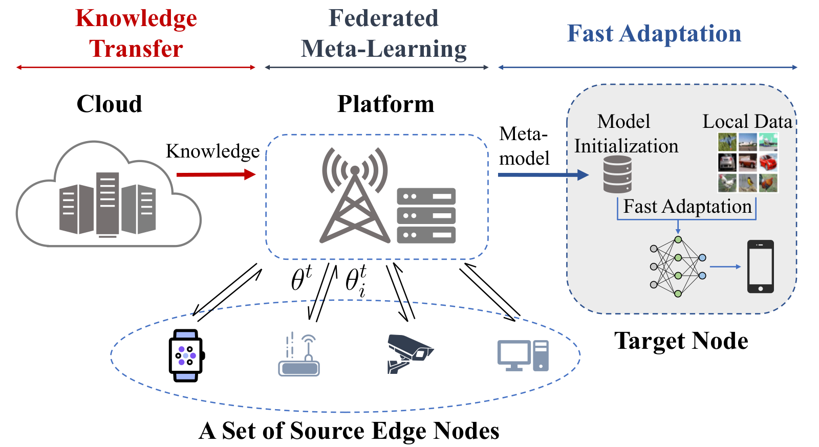
We consider a platform-aided federated meta-learning architecture for edge learning (as illustrated in Figure 1), where a set ℐ\mathcal{I} of source edge nodes joint force to learn a meta-model, aided by the valuable knowledge learned from previous tasks in the cloud. Specifically, the knowledge transfer is in the form of regularization using Bregman divergence on the prior model.
Refer to caption
Figure 1. Illustration of the platform-aided federated meta-learning architecture with knowledge transfer.

3.1. Problem Formulation

For ease of exposition, we consider a general supervised learning setting where each edge node i∈ℐ∪{m}i\in\mathcal{I}\cup\{m\} has a labeled dataset 𝒟i={(𝐱ij,𝐲ij)}j=1Di\mathcal{D}_{i}=\big\{(\mathbf{x}^{j}_{i},\mathbf{y}^{j}_{i})\big\}^{D_{i}}_{j=1} with total DiD_{i} samples. Here (𝐱ij,𝐲ij)∈𝒳i×𝒴i(\mathbf{x}^{j}_{i},\mathbf{y}^{j}_{i})\in\mathcal{X}_{i}\times\mathcal{Y}_{i} is a sample point with input 𝐱ij\mathbf{x}^{j}_{i} and true label 𝐲ij\mathbf{y}^{j}_{i}, and follows an unknown underlying distribution PiP_{i}. For a model parameter ϕi∈ℝn\phi_{i}\in\mathbb{R}^{n}, the empirical loss function for a dataset 𝒟i\mathcal{D}_{i} is defined as Li​(ϕi,𝒟i)≜(1/Di)​∑j=1Dili​(ϕi,(𝐱ij,𝐲ij))L_{i}(\phi_{i},\mathcal{D}_{i})\triangleq(1/D_{i})\sum^{D_{i}}_{j=1}l_{i}\big(\phi_{i},(\mathbf{x}^{j}_{i},\mathbf{y}^{j}_{i})\big), where li​(⋅,⋅)l_{i}(\cdot,\cdot) is a general differentiable non-convex loss function.

Motivated by the recent success of regularization approaches in transfer learning and continual learning (Parisi et al. 2019), we use regularization for extracting the valuable knowledge from the prior model to facilitate fast edge training and to alleviate catastrophic forgetting. More specially, for a model parameter θ∈ℝn\theta\in\mathbb{R}^{n}, we denote θp∈ℝn\theta_{p}\in\mathbb{R}^{n} as the prior model parameter, and use the Bregman divergence Dh​(θ,θp)D_{h}(\theta,\theta_{p}) (Bregman 1967) as the regularization, given by:

(1) Dh​(θ,θp)≜h⁡(θ)−h⁡(θp)−⟨∇h​(θp),θ−θp⟩,\displaystyle D_{h}(\theta,\theta_{p})\triangleq h(\theta)-h(\theta_{p})-\langle\nabla h\big(\theta_{p}\big),\theta-\theta_{p}\rangle,

for some continuously-differentiable strictly convex function h⁡(⋅)h(\cdot). It is worth noting that Bregman divergence is a dissimilarity measure between two objects (e.g., vectors, matrices, distributions, etc.). It encompasses a rich class of divergence metrics, including squared Euclidean distance, squared Mahalanobis distance, Kullback-Leibler (KL) divergence, and Itakura-Saito (IS) distance, which are widely used in machine learning to encode the dissimilarity from different perspectives, and is particularly useful for the regularization approaches (Si et al. 2009; Yu et al. 2013; Jung et al. 2016). Note that while for ease of exposition, in this paper we consider the regularizer on the model parameters using Bregman divergence, the same methodology can be applied to generalize the regularization to be in terms of Bregman divergence between two functions of θ\theta and θp\theta_{p}, respectively (see Assumption 2).

Following the same line as in MAML (Finn et al. 2017), we divide the dataset 𝒟i\mathcal{D}_{i} for the source edge node i∈ℐi\in\mathcal{I} into two disjoint sets, i.e., the support set 𝒟is\mathcal{D}^{s}_{i} and the query set 𝒟iq\mathcal{D}^{q}_{i}. Based on the prior model, we can formulate the federated meta-learning with knowledge transfer among the source edge nodes as the following regularized optimization problem:

(2) minθ\displaystyle\min_{\theta} ∑i∈ℐwi​Li​(ϕi​(θ),𝒟iq)+λ​Dh​(θ,θp)\displaystyle\quad\sum_{i\in\mathcal{I}}w_{i}L_{i}\big(\phi_{i}(\theta),\mathcal{D}^{q}_{i}\big)+\lambda D_{h}(\theta,\theta_{p})
s.t. ϕi(θ)=θ−α∇Li(θ,𝒟si),i∈ℐ\displaystyle\quad\begin{array}[]{lr}\phi_{i}(\theta)=\theta-\alpha\nabla L_{i}(\theta,\mathcal{D}^{s}_{i}),~i\in\mathcal{I}\end{array}

where wi≜Di/∑i∈ℐDiw_{i}\triangleq D_{i}/\sum_{i\in\mathcal{I}}D_{i}, α\alpha is the learning rate, and λ\lambda is a penalty parameter that can be used to balance the trade-off between the loss and the regularization. In this formulation, we aim to find a good meta-model such that slight updating, i.e., one-step gradient descent, results in substantial performance improvement for any task across the edge nodes. That is, the source edge nodes collaboratively learn how to learn fast with a few data samples. Further, by penalizing changes in the model via regularization, the learned model from (2)-(3.1) is confined to stay ‘close’ to the prior model for enabling collaborative edge learning without forgetting prior knowledge, thus the learned meta-model can widely adapt to different types of tasks.

In the fast adaptation stage, the platform transfers the learned meta-model θ\theta to the target node (denoted by mm) after solving the regularized federated meta-learning problem (2)-(3.1). Based on θ\theta, the target node mm can use its local data set 𝒟ms\mathcal{D}^{s}_{m} to quickly compute a new model ϕm\phi_{m} by performing one-step stochastic gradient descent, i.e.,

(4) ϕm=θ−α∇Lm(θ,𝒟ms).\displaystyle\phi_{m}=\theta-\alpha\nabla L_{m}(\theta,\mathcal{D}^{s}_{m}).

Note that the target node also can execute a few steps of stochastic gradient descent updates for better performance when needed.

3.2. An Inexact-ADMM Based Algorithm for Regularized Federated Meta-Learning

As alluded to earlier, general gradient-based federated meta-learning approaches cannot handle the regularized optimization problem (2)-(3.1) well. To address this problem, we propose an inexact-ADMM based federated meta-learning algorithm (ADMM-FedMeta) to solve (2)-(3.1).

Observe that the federated meta-learning problem (2)-(3.1) is equivalent to the following constrained optimization problem:

(5) min{θi},θ∑i∈ℐwi​Li​(ϕi​(θi),𝒟iq)+λ​Dh​(θ,θp)s.t.θi−θ=0,i∈ℐ\displaystyle\begin{split}\min_{\{\theta_{i}\},\theta}&\quad\sum_{i\in\mathcal{I}}w_{i}L_{i}\big(\phi_{i}(\theta_{i}),\mathcal{D}^{q}_{i}\big)+\lambda D_{h}(\theta,\theta_{p})\\ \text{s.t.}\,&\quad\begin{array}[]{lr}\theta_{i}-\theta=0,~i\in\mathcal{I}\\ \end{array}\end{split}

where ϕi​(θi)\phi_{i}(\theta_{i}) is given by (3.1). To solve (5), we form the augmented Lagrangian function as follows:

ℒ⁡({θi,yi},θ)≜\displaystyle\mathcal{L}\big(\{\theta_{i},y_{i}\},\theta\big)\triangleq ∑i∈ℐ(wi​Li​(ϕi​(θi),𝒟iq)+⟨yi,θi−θ⟩CLOSE\displaystyle\sum_{i\in\mathcal{I}}\Big(w_{i}L_{i}\big(\phi_{i}(\theta_{i}),\mathcal{D}^{q}_{i}\big)+\langle y_{i},\theta_{i}-\theta\rangle
(6) OPEN+ρi2​‖θi−θ‖2)+λ​Dh​(θ,θp),\displaystyle+\frac{\rho_{i}}{2}\|\theta_{i}-\theta\|^{2}\Big)+\lambda D_{h}(\theta,\theta_{p}),

where yi∈ℝny_{i}\in\mathbb{R}^{n} is a dual variable and ρi>0\rho_{i}>0 is a penalty parameter for each i∈ℐi\in\mathcal{I}.

When the classical ADMM method is applied (Boyd et al. 2011), the variables θi\theta_{i}, θ\theta and yiy_{i} are updated alternatively in solving (5) as follows:

(7) {θt+1=arg​minθ⁡ℒ​({θit,yit},θ),θit+1=arg​minθi⁡ℒi​(θi,yit,θt+1),yit+1=yit+ρi​(θit+1−θt+1),\displaystyle\begin{cases}\theta^{t+1}=\argmin_{\theta}~\mathcal{L}\big(\{\theta^{t}_{i},y^{t}_{i}\},\theta\big),\\ \theta^{t+1}_{i}=\argmin_{\theta_{i}}~\mathcal{L}_{i}\big(\theta_{i},y^{t}_{i},\theta^{t+1}\big),\\ y^{t+1}_{i}=y^{t}_{i}+\rho_{i}(\theta^{t+1}_{i}-\theta^{t+1}),\\ \end{cases}

where ℒi​(θi,yi,θ)≜wi​Li​(ϕi​(θi),𝒟iq)+⟨yi,θi−θ⟩+ρi2​‖θi−θ‖2\mathcal{L}_{i}\big(\theta_{i},y_{i},\theta\big)\triangleq w_{i}L_{i}\big(\phi_{i}(\theta_{i}),\mathcal{D}^{q}_{i}\big)+\langle y_{i},\theta_{i}-\theta\rangle+\frac{\rho_{i}}{2}\|\theta_{i}-\theta\|^{2}. The conventional ADMM decomposes the problem (5) into a set of subproblems that can be solved in parallel, while computing Dh​(θ,θp)D_{h}(\theta,\theta_{p}) and Li​(ϕi​(θi),𝒟iq)L_{i}\big(\phi_{i}(\theta_{i}),\mathcal{D}^{q}_{i}\big) separately. Based on that, to fully take advantage of the combined computation power of the local edge nodes and the platform, we provide the following alternating updating strategy: 1) updating θ\theta at the platform and 2) updating {θi,yi}\{\theta_{i},y_{i}\} at the source edge nodes in a distributed manner. Particularly, in this way, the computation corresponding to the regularizer can be decoupled from the edge nodes to the the platform. However, attaining the exact solution to each subproblem is computationally costly, especially with a complex DNN model. To tackle this challenge, we devise the inexact-ADMM based federated meta-learning (ADMM-FedMeta) below.

Specifically, in communication round t=0t=0, the platform initializes θ0\theta^{0} and sends it to all edge nodes. Each node i∈ℐi\in\mathcal{I} initializes yi−1y^{-1}_{i} locally.

  • •

    Local update of {θi,yi}\bm{\{\theta_{i},y_{i}\}}. After receiving θt\theta^{t} from the platform at communication round tt, each edge node i∈ℐi\in\mathcal{I} would do the following updates:

    (1) Update node-specific model ϕi\phi_{i}. Based on the dataset 𝒟is\mathcal{D}^{s}_{i}, ϕit\phi^{t}_{i} is updated as:

    (8) ϕit=θt−α∇Li(θt,𝒟is).\displaystyle\phi^{t}_{i}=\theta^{t}-\alpha\nabla L_{i}(\theta^{t},\mathcal{D}^{s}_{i}).

    (2) Update local parameter θi\theta_{i}. Based on (7), given the meta-model θt\theta^{t} and local dual variable yit−1y_{i}^{t-1} from last communication round, the local parameter θi\theta_{i} should be updated as:

    θit=\displaystyle\theta^{t}_{i}= arg⁡minθi{wiLi(ϕi(θi),𝒟iq)+⟨yit−1,θi−θt⟩\displaystyle\mathop{\arg\min}_{\theta_{i}}\bigg\{w_{i}L_{i}\big(\phi_{i}(\theta_{i}),\mathcal{D}^{q}_{i}\big)+\langle y^{t-1}_{i},\theta_{i}-\theta^{t}\rangle
    (9) +ρi2∥θi−θt∥2}.\displaystyle+\frac{\rho_{i}}{2}\|\theta_{i}-\theta^{t}\|^{2}\bigg\}.

    To simplify the computation, we use linear approximation (i.e., first-order Taylor expansion) around θt\theta^{t} to relax this subproblem, i.e.,

    θit=\displaystyle\theta^{t}_{i}= arg⁡minθi{wiLi(ϕit,𝒟iq)\displaystyle\mathop{\arg\min}_{\theta_{i}}\bigg\{w_{i}L_{i}(\phi^{t}_{i},\mathcal{D}^{q}_{i})
    +⟨wi(I−α∇2Li(θt,𝒟is))∇Li(ϕit,𝒟iq)\displaystyle+\big\langle w_{i}\big(I-\alpha\nabla^{2}L_{i}(\theta^{t},\mathcal{D}^{s}_{i})\big)\nabla L_{i}(\phi^{t}_{i},\mathcal{D}^{q}_{i})
    (10) +yit−1,θi−θt⟩+ρi2∥θi−θt∥2},\displaystyle+y^{t-1}_{i},\theta_{i}-\theta^{t}\big\rangle+\frac{\rho_{i}}{2}\|\theta_{i}-\theta^{t}\|^{2}\bigg\},

    where ϕit\phi^{t}_{i} is from (8). Nevertheless, (• ‣ 3.2) is still insufficient since the computational complexity of the Hessian-gradient product ∇2Li(θt,𝒟is)∇Li(ϕit,𝒟iq)\nabla^{2}L_{i}(\theta^{t},\mathcal{D}^{s}_{i})\nabla L_{i}\big(\phi^{t}_{i},\mathcal{D}^{q}_{i}\big) is 𝒪⁡(n2)\mathcal{O}(n^{2}). To further reduce the computational cost, as in (Fallah et al. 2020a; Ji et al. 2020), we replace the Hessian-gradient product by a first-order estimator, i.e.,

    (11) git≜∇Li​(θt+δi,t​rit,𝒟is)−∇Li​(θt−δi,t​rit,𝒟is)2​δi,t,\displaystyle g^{t}_{i}\triangleq\frac{\nabla L_{i}\big(\theta^{t}+\delta_{i,t}r^{t}_{i},\mathcal{D}^{s}_{i}\big)-\nabla L_{i}\big(\theta^{t}-\delta_{i,t}r^{t}_{i},\mathcal{D}^{s}_{i}\big)}{2\delta_{i,t}},

    where rit≜∇Li​(ϕit,𝒟iq)r^{t}_{i}\triangleq\nabla L_{i}\big(\phi^{t}_{i},\mathcal{D}^{q}_{i}\big) and δi,t>0\delta_{i,t}>0 is the degree of freedom capturing the estimation accuracy. In a nutshell, the local parameter θit\theta_{i}^{t} is updated as follows:

    (12) θit=θt−yit−1+wi​(∇Li​(ϕit,𝒟iq)−α​git)ρi,\displaystyle\theta^{t}_{i}=\theta^{t}-\frac{y^{t-1}_{i}+w_{i}\big(\nabla L_{i}(\phi^{t}_{i},\mathcal{D}^{q}_{i})-\alpha g^{t}_{i}\big)}{\rho_{i}},

    where (12) is derived by the optimality of (• ‣ 3.2) after replacing ∇2Li(θt,𝒟is)∇Li(ϕit,𝒟iq)\nabla^{2}L_{i}(\theta^{t},\mathcal{D}^{s}_{i})\nabla L_{i}\big(\phi^{t}_{i},\mathcal{D}^{q}_{i}\big) with gitg^{t}_{i}.

    (3) Update local dual variable yiy_{i}. Based on θt\theta^{t} and the updated local parameter θit\theta_{i}^{t}, the auxiliary dual variable yity_{i}^{t} is next updated according to:

    (13) yit=\displaystyle y^{t}_{i}= yit−1+ρi​(θit−θt).\displaystyle y^{t-1}_{i}+\rho_{i}(\theta^{t}_{i}-\theta^{t}).
  • •

    Global Aggregation towards Meta-Model θ\bm{\theta}. Each edge node i∈ℐi\in\mathcal{I} sends the updated local parameters θit\theta^{t}_{i} and yity^{t}_{i} to the platform. With the prior model θp\theta_{p} transferred from the cloud, the platform performs a global update of the model initialization θ\theta based on:

    (14) θt+1=∑i∈ℐ(yit+ρi​θit)−λ​∇θtDh​(θt,θp)∑i∈ℐρi,\displaystyle\theta^{t+1}=\frac{\sum_{i\in\mathcal{I}}(y^{t}_{i}+\rho_{i}\theta^{t}_{i})-\lambda\nabla_{\theta^{t}}D_{h}(\theta^{t},\theta_{p})}{\sum_{i\in\mathcal{I}}\rho_{i}},

    where (14) is derived from the optimality of the linearized ℒ⁡({θit,yit},θ)\mathcal{L}\big(\{\theta^{t}_{i},y^{t}_{i}\},\theta\big) around θt\theta^{t} similar to (12). Then, the platform sends θt+1\theta^{t+1} back to all edge nodes for the next communication round.

  • •

    Fast Adaptation. After the training phase, the platform transfers the learned meta-model θT\theta^{T} to the target node mm. Based on θT\theta^{T}, the target node performs one or a few steps of stochastic gradient descent on its own dataset to obtain a new model.

The details of ADMM-FedMeta are summarized in Algorithm 1. Note that due to linearizing all decomposed subproblems and estimating Hessian by its first-order estimation, we enable the computation complexity of ADMM-FedMeta to be 𝒪⁡(n)\mathcal{O}(n) per round, which maintains the lowest among all existing federated meta-learning approaches.

Input: θp\theta_{p}, α\alpha, λ\lambda, ρi\rho_{i}, 𝒟is\mathcal{D}^{s}_{i}, 𝒟iq\mathcal{D}^{q}_{i} for i∈ℐi\in\mathcal{I}
Output: Finial meta-model θ\theta
Each edge node i∈ℐi\in\mathcal{I} initializes yi−1y^{-1}_{i}; 1
Platform initializes θ0\theta^{0} and sends it to all edge nodes; 2
for t=0t=0 to TT do 3
for i=1i=1 to II do 4
    Compute ϕit←θt−α∇Li(θt,𝒟is)\phi^{t}_{i}\leftarrow\theta^{t}-\alpha\nabla L_{i}(\theta^{t},\mathcal{D}^{s}_{i}); 5
       Compute θit\theta^{t}_{i} by (12); 6
       Compute yit←yit−1+ρi​(θit−θt)y^{t}_{i}\leftarrow y^{t-1}_{i}+\rho_{i}(\theta^{t}_{i}-\theta^{t}); 7
       Send θit\theta^{t}_{i} and yity^{t}_{i} back to the platform; 8
       end for 9
   Platform updates θt+1\theta^{t+1} by (14) and sends it to all edge nodes i∈ℐi\in\mathcal{I}; 10
    end for 11
Platform transfers θT\theta^{T} to target node for fast adaptation; 12
Algorithm 1 Inexact-ADMM Based Meta-Learning Algorithm (ADMM-FedMeta)

4. Performance Analysis

In this section, we analyze the performance of ADMM-FedMeta. First, we study the convergence properties and characterize the communication complexity for ADMM-FedMeta. Then, we quantify the forgetting effect to previous tasks of the meta-model and analyze the fast adaptation performance at the target edge node.

4.1. Convergence Analysis

For convenience, we denote the objective function of (2) as F⁡(θ)F(\theta):

(15) F⁡(θ)≜∑i∈ℐwi​Li​(ϕi​(θ),𝒟iq)+λ​Dh​(θ,θp),\displaystyle F(\theta)\triangleq\sum_{i\in\mathcal{I}}w_{i}L_{i}\big(\phi_{i}(\theta),\mathcal{D}^{q}_{i}\big)+\lambda D_{h}(\theta,\theta_{p}),

where ϕi(θ)=θ−α∇Li(θ,𝒟is)\phi_{i}(\theta)=\theta-\alpha\nabla L_{i}(\theta,\mathcal{D}^{s}_{i}). Next, we characterize the convergence and communication complexity of the proposed algorithm for finding a first-order stationary point of function F⁡(θ)F(\theta). Formally, the definition of an ϵ\epsilon-approximate first-order stationary point is given as follows.

Definition 0 (ϵ\epsilon-FOSP).

A solution θ∈ℝn\theta\in\mathbb{R}^{n} is called an ϵ\epsilon-approximate first-order stationary point (ϵ\epsilon-FOSP) of (2), if ‖∇F​(θ)‖≤ϵ,for​ϵ>0\|\nabla F(\theta)\|\leq\epsilon,~\text{for}~\epsilon>0.

The above definition implies that if a solution θ\theta obtained by an algorithm is a ϵ\epsilon-FOSP, then the gradient norm of the objective function is bounded above by ϵ\epsilon.

Note that the first-order estimator of Hessian introduced in the subproblem (12) inevitably complicates the convergence analysis of ADMM-FedMeta, making the existing analysis methods of ADMM (Barber and Sidky 2020) not suitable here. To establish the convergence of ADMM-FedMeta, we impose the following standard assumptions in the literature.

Assumption 1.

F⁡(θ)F(\theta) is lower-bounded, i.e., F⁡(θ)>−∞F(\theta)>-\infty, for all θ∈ℝn\theta\in\mathbb{R}^{n}.

Assumption 2 (Smoothness and Bounded Gradient).

For each i∈ℐ∪{m}i\in\mathcal{I}\cup\{m\}, any 𝒟is\mathcal{D}^{s}_{i}, and θp∈ℝn\theta_{p}\in\mathbb{R}^{n}, both Li​(⋅,𝒟is)L_{i}(\cdot,\mathcal{D}^{s}_{i}) and Dh​(⋅,θp)D_{h}(\cdot,\theta_{p}) are twice continuously differentiable and smooth, i.e., for any x,y∈ℝnx,y\in\mathbb{R}^{n}, there exist constants μi>0\mu_{i}>0 and μr>0\mu_{r}>0 such that:

(16) ‖∇Li​(x,𝒟is)−∇Li​(y,𝒟is)‖≤μi​‖x−y‖,\displaystyle\|\nabla L_{i}(x,\mathcal{D}^{s}_{i})-\nabla L_{i}(y,\mathcal{D}^{s}_{i})\|\leq\mu_{i}\|x-y\|,
(17) ‖∇xDh​(x,θp)−∇yDh​(y,θp)‖≤μr​‖x−y‖.\displaystyle\|\nabla_{x}D_{h}(x,\theta_{p})-\nabla_{y}D_{h}(y,\theta_{p})\|\leq\mu_{r}\|x-y\|.

Besides, the gradient norms of Li​(⋅,𝒟is)L_{i}(\cdot,\mathcal{D}^{s}_{i}) is bounded by a positive constant βi>0\beta_{i}>0, i.e., for any x∈ℝnx\in\mathbb{R}^{n}, the following holds:

(18) ‖∇Li​(x,𝒟is)‖≤βi.\displaystyle\|\nabla L_{i}(x,\mathcal{D}^{s}_{i})\|\leq\beta_{i}.
Assumption 3 (Lipschitz Continuous Hessian).

For any i∈ℐi\in\mathcal{I} and any 𝒟is\mathcal{D}^{s}_{i}, the Hessian of Li​(⋅,𝒟is)L_{i}(\cdot,\mathcal{D}^{s}_{i}) is ζi\zeta_{i}-Lipschitz continuous, i.e., for any x,y∈ℝnx,y\in\mathbb{R}^{n}, we have:

(19) ‖∇2Li​(x,𝒟is)−∇2Li​(y,𝒟is)‖≤ζi​‖x−y‖.\displaystyle\|\nabla^{2}L_{i}(x,\mathcal{D}^{s}_{i})-\nabla^{2}L_{i}(y,\mathcal{D}^{s}_{i})\|\leq\zeta_{i}\|x-y\|.
Assumption 4 (Bounded Variance).

For any i∈ℐ∪{m}i\in\mathcal{I}\cup\{m\} and θ∈ℝn\theta\in\mathbb{R}^{n}, the stochastic gradient ∇li​(θ,(𝐱,𝐲))\nabla l_{i}\big(\theta,(\mathbf{x},\mathbf{y})\big) and Hessian ∇2li​(θ,(𝐱,𝐲))\nabla^{2}l_{i}\big(\theta,(\mathbf{x},\mathbf{y})\big) with respect to data point (𝐱,𝐲)∈𝒳i×𝒴i(\mathbf{x},\mathbf{y})\in\mathcal{X}_{i}\times\mathcal{Y}_{i} have bounded variances, i.e.,

(20) 𝔼(𝐱,𝐲)∼Pi​{‖∇li​(θ,(𝐱,𝐲))−∇Li​(θ)‖2}≤(σig)2,\displaystyle\mathbb{E}_{(\mathbf{x},\mathbf{y})\sim P_{i}}\big\{\|\nabla l_{i}\big(\theta,(\mathbf{x},\mathbf{y})\big)-\nabla L_{i}(\theta)\|^{2}\big\}\leq\big(\sigma^{g}_{i}\big)^{2},
(21) 𝔼(𝐱,𝐲)∼Pi​{‖∇2li​(θ,(𝐱,𝐲))−∇2Li​(θ)‖2}≤(σih)2,\displaystyle\mathbb{E}_{(\mathbf{x},\mathbf{y})\sim P_{i}}\big\{\|\nabla^{2}l_{i}\big(\theta,(\mathbf{x},\mathbf{y})\big)-\nabla^{2}L_{i}(\theta)\|^{2}\big\}\leq\big(\sigma^{h}_{i}\big)^{2},

for some positive constants σig>0\sigma^{g}_{i}>0 and σih>0\sigma^{h}_{i}>0.

Assumptions 1-4 are standard in the state-of-the-art studies on the analysis of federated learning algorithms (Lin et al. 2020; Fallah et al. 2020b; Zhang et al. 2020a). In particular, (18) is critical for analyzing the convergence as it enables characterizing the estimation error of the Hessian. Assumption 3 implies the high-order smoothness of Li​(⋅,𝒟is)L_{i}(\cdot,\mathcal{D}^{s}_{i}) for dealing with the second-order information in the update steps of Algorithm 1. Furthermore, Assumption 4 provides the upper bounds of the variances of the gradient and Hessian estimations.

To quantify the convergence behavior of ADMM-FedMeta, we first study the properties of the objective function F⁡(θ)F(\theta). Denote Fi​(θ)≜Li​(ϕi​(θ),𝒟iq)F_{i}(\theta)\triangleq L_{i}\big(\phi_{i}(\theta),\mathcal{D}^{q}_{i}\big). Based on Assumptions 2 and 3, we have the following result about the smoothness of FiF_{i} as in the standard analysis of federated meta-learning approaches.

Lemma 0.

Given Assumptions 2 and 3, for each i∈ℐ∪{m}i\in\mathcal{I}\cup\{m\}, FiF_{i} is proper and νi\nu_{i}-smooth, i.e.,

(22) ‖∇Fi​(x)−∇Fi​(y)‖≤νi​‖x−y‖,∀x,y∈ℝn,\displaystyle\|\nabla F_{i}(x)-\nabla F_{i}(y)\|\leq\nu_{i}\|x-y\|,~\forall x,y\in\mathbb{R}^{n},

where νi\nu_{i} is defined as follows:

(23) νi≜(1+α​μi)​(1+μi)​μi+α​βi​ζi.\displaystyle\nu_{i}\triangleq(1+\alpha\mu_{i})(1+\mu_{i})\mu_{i}+\alpha\beta_{i}\zeta_{i}.
Proof.

The proof is standard. The detailed proof is provided in Appendix A of the technical report (Yue et al. 2020). ∎

Next, we impose the assumptions on the hyper-parameters.

Assumption 5.

For all i∈ℐi\in\mathcal{I}, ρi\rho_{i} is large enough such that:

(24) ρi2−4​wi​νi>0,\displaystyle\frac{\rho_{i}}{2}-4w_{i}\nu_{i}>0,
(25) ρi2−2​wi2​νi2​(4​wi​νiρi2+1ρi)−λ​μr2​I>0,\displaystyle\frac{\rho_{i}}{2}-2w^{2}_{i}\nu^{2}_{i}\bigg(\frac{4w_{i}\nu_{i}}{\rho^{2}_{i}}+\frac{1}{\rho_{i}}\bigg)-\frac{\lambda\mu_{r}}{2I}>0,
(26) ρi−3​νi>0,\displaystyle\rho_{i}-3\nu_{i}>0,

where νi\nu_{i} is a smooth scalar defined in (23). Besides, for all i∈ℐi\in\mathcal{I}, the additional degree of freedom parameter {δi,t}\{\delta_{i,t}\} for the approximation of Hessian-gradient products is chosen to be a monotonically non-increasing positive sequence and satisfies ∑t=1∞δi,t<∞\sum^{\infty}_{t=1}\delta_{i,t}<\infty.

We impose Assumption 5 on the penalty parameter ρi\rho_{i} and the degree of freedom parameter δi,t\delta_{i,t}. Intuitively, (24)-(26) imply that a large ρi\rho_{i} is required to balance the error caused by the linear approximation and Hessian estimation in (12).

Based on Lemma 2, we are ready to establish the convergence and characterize the communication complexity for Algorithm 1.

Theorem 3 (Convergence and Communication Complexity).

Under Assumptions 1-5, we have the following results based on Algorithm 1:

  1. (i)

    {θt}\{\theta^{t}\} has at least one limit point and each limit point θ∗\theta^{*} is a stationary solution of (2), i.e., ‖∇F​(θ∗)‖=0\|\nabla F(\theta^{*})\|=0.

  2. (ii)

    Algorithm 1 finds an ϵ\epsilon-FOSP of Problem (2)-(3.1) after at most 𝒪⁡(1/ϵ2)\mathcal{O}(1/\epsilon^{2}) communication rounds.

Proof.

For part (i), we first characterize the successive difference of the augmented Lagrangian function. Based on that, we next show limt→∞‖θit+1−θit‖=0\lim_{t\rightarrow\infty}\|\theta^{t+1}_{i}-\theta^{t}_{i}\|=0 and limt→∞‖θt+1−θt‖=0\lim_{t\rightarrow\infty}\|\theta^{t+1}-\theta^{t}\|=0. Lastly, we bound ‖∇F​(θt)‖\|\nabla F(\theta^{t})\| via ‖θit+1−θit‖\|\theta^{t+1}_{i}-\theta^{t}_{i}\| and ‖θt+1−θt‖\|\theta^{t+1}-\theta^{t}\|. We prove (ii) via dividing the sum of the Lagrangian successive difference into two finite parts. The detailed proof is presented in Appendix F of the technical report (Yue et al. 2020). ∎

Theorem 3 indicates that Algorithm 1 always converges to a stationary point of (2). Besides, to find an ϵ\epsilon-FOSP of Problem (2)-(3.1), Algorithm 1 requires 𝒪⁡(1/ϵ2)\mathcal{O}(1/\epsilon^{2}) communication rounds between edge nodes and the platform. It is worth noting that in contrast to the previous methods (Lin et al. 2020; Fallah et al. 2020b; Fallah et al. 2020a), ADMM-FedMeta can converge under mild conditions, i.e., not depending on the similarity assumptions (i.e., Assumption 6) across different edge nodes. This implies that Algorithm 1 can be applied to unbalanced and heterogeneous local datasets, revealing the potential in dealing with the inherent challenges in federated learning.

To characterize the impact of local data samples on the expected performance on the source nodes, we provide the following corollary.

Corollary 0.

Given Assumptions 1-5, the ϵ\epsilon-FOSP solution θϵ\theta_{\epsilon} found by Algorithm 1 satisfies that:

𝔼{∥∑i∈ℐwiLi(θϵ−α∇Li(θϵ))+λDh(θϵ,θp)∥}\displaystyle\mathbb{E}\Big\{\Big\|\sum_{i\in\mathcal{I}}w_{i}L_{i}\big(\theta_{\epsilon}-\alpha\nabla L_{i}(\theta_{\epsilon})\big)+\lambda D_{h}(\theta_{\epsilon},\theta_{p})\Big\|\Big\}
(27) ≤ϵ+∑i∈ℐwi​σig​(α​μiDis+1Diq),\displaystyle\leq\epsilon+\sum_{i\in\mathcal{I}}w_{i}\sigma^{g}_{i}\Bigg(\frac{\alpha\mu_{i}}{\sqrt{D^{s}_{i}}}+\frac{1}{\sqrt{D^{q}_{i}}}\Bigg),

where wi=1/Iw_{i}=1/I and Li​(⋅)L_{i}(\cdot) is the expected loss denoted by:

(28) Li​(θ)≜𝔼(𝐱,𝐲)∼Pi​{li​(θ,(𝐱,𝐲))}.\displaystyle L_{i}(\theta)\triangleq\mathbb{E}_{(\mathbf{x},\mathbf{y})\sim P_{i}}\big\{l_{i}\big(\theta,(\mathbf{x},\mathbf{y})\big)\big\}.
Proof.

The detailed proof is presented in Appendix G of the technical report (Yue et al. 2020). ∎

Corollary 4 implies that despite ϵ\epsilon-FOSP of the deterministic loss (2) can be obtained within 𝒪⁡(1/ϵ2)\mathcal{O}(1/\epsilon^{2}) rounds, performance degradation may happen due to small sample size.

4.2. Performance of Rapid Adaptation at Target Node

While the task similarity assumption is not required to guarantee the convergence of Algorithm 1, we impose such an assumption to study the fast adaptation performance at the target node mm.

Assumption 6 (Task Similarity).

There exist positive constants ψig>0\psi^{g}_{i}>0 and ψih>0\psi^{h}_{i}>0 such that for any i∈ℐi\in\mathcal{I} and θ∈ℝn\theta\in\mathbb{R}^{n}, the following holds:

(29) ‖∇Lm​(θ)−∇Li​(θ)‖≤ψig,\displaystyle\|\nabla L_{m}(\theta)-\nabla L_{i}(\theta)\|\leq\psi^{g}_{i},
(30) ‖∇2Lm​(θ)−∇2Li​(θ)‖≤ψih,\displaystyle\|\nabla^{2}L_{m}(\theta)-\nabla^{2}L_{i}(\theta)\|\leq\psi^{h}_{i},

where Li​(⋅)L_{i}(\cdot) is defined in (28), and the same applies to Lm​(⋅)L_{m}(\cdot).

Assumption 6 indicates that the variations of the gradients between the loss of source edge nodes and the target edge node are bounded by some constants, which capture the similarity of the tasks corresponding to non-IID data and holds for many practical loss functions (Zhang et al. 2020a), such as logistic regression and hyperbolic tangent functions. In particular, ψig\psi^{g}_{i} and ψih\psi^{h}_{i} can be roughly seen as a distance between data distributions PmP_{m} and PiP_{i} (Fallah et al. 2020a).

Next, we present the following result about the performance of rapid adaptation.

Theorem 5 (Fast Adaptation Performance).

Suppose that Assumptions 1-6 hold. For any ϵ>0\epsilon>0, the ϵ\epsilon-FOSP solution θϵ\theta_{\epsilon} obtained by Algorithm 1 satisfies that:

𝔼⁡{‖∇Fm​(θϵ)‖}≤\displaystyle\mathbb{E}\big\{\|\nabla F_{m}(\theta_{\epsilon})\|\big\}\leq ϵ+α​βm​∑i∈ℐwi​ψih+(α​μ+1)2​∑i∈ℐwi​ψig\displaystyle\epsilon+\alpha\beta_{m}\sum_{i\in\mathcal{I}}w_{i}\psi^{h}_{i}+(\alpha\mu+1)^{2}\sum_{i\in\mathcal{I}}w_{i}\psi^{g}_{i}
+αμ(αμ+1)∑i∈ℐwiσig(1Dmq+1Diq)\displaystyle+\alpha\mu(\alpha\mu+1)\sum_{i\in\mathcal{I}}w_{i}\sigma^{g}_{i}\Bigg(\frac{1}{\sqrt{D^{q}_{m}}}+\frac{1}{\sqrt{D^{q}_{i}}}\Bigg)
+(αμ+1)∑i∈ℐwiσig(1Dms+1Dis)\displaystyle+(\alpha\mu+1)\sum_{i\in\mathcal{I}}w_{i}\sigma^{g}_{i}\Bigg(\frac{1}{\sqrt{D^{s}_{m}}}+\frac{1}{\sqrt{D^{s}_{i}}}\Bigg)
(31) +αβm∑i∈ℐwiσih(1Dms+1Dis),\displaystyle+\alpha\beta_{m}\sum_{i\in\mathcal{I}}w_{i}\sigma^{h}_{i}\Bigg(\frac{1}{\sqrt{D^{s}_{m}}}+\frac{1}{\sqrt{D^{s}_{i}}}\Bigg),

where Fm(θ)≜Lm(θ−α∇Lm(θ,𝒟ms),𝒟mq)+λDh(θ,θp)F_{m}(\theta)\triangleq L_{m}\big(\theta-\alpha\nabla L_{m}(\theta,\mathcal{D}^{s}_{m}),\mathcal{D}^{q}_{m}\big)+\lambda D_{h}(\theta,\theta_{p}) for any 𝒟ms\mathcal{D}^{s}_{m} and 𝒟mq\mathcal{D}^{q}_{m} with respect to distribution PmP_{m}, and μ=maxi∈ℐ⁡{μi}\mu=\max_{i\in\mathcal{I}}\{\mu_{i}\}.

Proof.

The detailed proof is presented in Appendix H of the technical report (Yue et al. 2020). ∎

Theorem 5 sheds light on the performance of fast adaptation with the previous knowledge, which depends on the size of datasets, the variance of stochastic gradient and Hessian, and the similarity between the target node and source nodes. In particular, if Dis=𝒪⁡(ϵ−2)D^{s}_{i}=\mathcal{O}(\epsilon^{-2}) and Diq=𝒪⁡(ϵ−2)D^{q}_{i}=\mathcal{O}(\epsilon^{-2}) for i∈ℐ∪{m}i\in\mathcal{I}\cup\{m\}, then an 𝒪⁡(ϵ+∑i∈ℐwi​(ψih+ψig))\mathcal{O}\big(\epsilon+\sum_{i\in\mathcal{I}}w_{i}(\psi^{h}_{i}+\psi^{g}_{i})\big)-FOSP can be obtained at the target node. However, it is clear that the larger the dataset of source nodes dissimilar to the target node is, the worse the rapid adaptation performs. In the next subsection, we will show these issues can be alleviated via regularization with a good prior model.

4.3. Forgetting effect on Prior Knowledge

In this section, we quantify the forgetting effect of the previous task of Algorithm 1 in a special case, where the regularizer is squared Euclidean distance, i.e., Dh​(θ,θp)=‖θ−θp‖2D_{h}(\theta,\theta_{p})=\|\theta-\theta_{p}\|^{2}. To do so, we first derive an upper bound of Dh​(θ,θp)D_{h}(\theta,\theta_{p}) via the following lemma.

Lemma 0.

Given Assumptions 1-5, for any ϵ>0\epsilon>0, the ϵ\epsilon-FOSP solution θϵ\theta_{\epsilon} obtained by Algorithm 1 satisfies that:

(32) 𝔼⁡{Dh​(θϵ,θp)}≤1λ​(ϵ+∑i∈ℐwi​(βi+α​μi​σigDis+σigDiq))​‖θϵ−θp‖.\displaystyle\mathbb{E}\big\{D_{h}(\theta_{\epsilon},\theta_{p})\big\}\leq\frac{1}{\lambda}\left(\epsilon+\sum_{i\in\mathcal{I}}w_{i}\left(\beta_{i}+\frac{\alpha\mu_{i}\sigma^{g}_{i}}{\sqrt{D^{s}_{i}}}+\frac{\sigma^{g}_{i}}{\sqrt{D^{q}_{i}}}\right)\right)\|\theta_{\epsilon}-\theta_{p}\|.

Particularly, suppose Dh​(θ,θp)D_{h}(\theta,\theta_{p}) is strongly convex with respect to θ\theta, i.e., there exists M>0M>0 such that for x,y∈ℝnx,y\in\mathbb{R}^{n}, the following holds:

(33) ⟨∇Dh​(x,θp)−∇Dh​(y,θp),x−y⟩≥M​‖x−y‖2.\displaystyle\left\langle\nabla D_{h}(x,\theta_{p})-\nabla D_{h}(y,\theta_{p}),x-y\right\rangle\geq M\|x-y\|^{2}.

Then (32) can be written as:

(34) 𝔼⁡{Dh​(θϵ,θp)}≤1M​λ2​(ϵ+∑i∈ℐwi​(βi+α​μi​σigDis+σigDiq))2.\displaystyle\mathbb{E}\big\{D_{h}(\theta_{\epsilon},\theta_{p})\big\}\leq\frac{1}{M\lambda^{2}}\left(\epsilon+\sum_{i\in\mathcal{I}}w_{i}\left(\beta_{i}+\frac{\alpha\mu_{i}\sigma^{g}_{i}}{\sqrt{D^{s}_{i}}}+\frac{\sigma^{g}_{i}}{\sqrt{D^{q}_{i}}}\right)\right)^{2}.
Proof.

The detailed proof is presented in Appendix I of the technical report (Yue et al. 2020). ∎

For a current model parameter θ\theta, we define the forgetting cost of θ\theta on the previous task pp as Lp​(θ)L_{p}(\theta) (Krishnan and Balaprakash 2020), where Lp​(⋅)L_{p}(\cdot) is the expected loss over the data distribution of task pp (defined by (28)). Based on Lemma 6, we next characterize the forgetting cost of the ϵ\epsilon-FOSP solution.

Theorem 7.

Suppose that Lp​(⋅)L_{p}(\cdot) is μp\mu_{p}-smooth, ‖∇Lp​(θp)‖≤ϵp\|\nabla L_{p}(\theta_{p})\|\leq\epsilon_{p} for some ϵp>0\epsilon_{p}>0, and Dh​(θ,θp)=‖θ−θp‖2D_{h}(\theta,\theta_{p})=\|\theta-\theta_{p}\|^{2}. Under Assumptions 1-5, for the ϵ\epsilon-FOSP solution θϵ\theta_{\epsilon}, we have the following result:

(35) ‖∇Lp​(θϵ)‖≤ϵp+νp2​λ​(ϵ+∑i∈ℐwi​(βi+α​μi​σigDis+σigDiq)).\displaystyle\|\nabla L_{p}(\theta_{\epsilon})\|\leq\epsilon_{p}+\frac{\nu_{p}}{2\lambda}\left(\epsilon+\sum_{i\in\mathcal{I}}w_{i}\left(\beta_{i}+\frac{\alpha\mu_{i}\sigma^{g}_{i}}{\sqrt{D^{s}_{i}}}+\frac{\sigma^{g}_{i}}{\sqrt{D^{q}_{i}}}\right)\right).
Proof.

The result can be directly obtained by Lemma 6. ∎

Based on Theorem 7 and corollary 4, it is clear that by selecting a suitable λ\lambda, the regularizer enables the meta-model to learn on the current task while maintaining good performance on the previous task. On the other hand, combined with Theorem 5, Theorem 7 also implies that due to the independence of (35) and similarity conditions, a good prior reference model (e.g., with a relatively small ‖∇Lm​(θp)‖\|\nabla L_{m}(\theta_{p})\|) can effectively alleviate the significant performance degradation caused by the dissimilarity between the source nodes and the target nodes.

5. Experimental Results

Dataset # local updates FedAvg Per-FedAvg ADMM-FedMeta
Fashion- MNIST 1 83.99%±3.90%83.99\%\pm 3.90\% 87.55%±2.42%87.55\%\pm 2.42\% 95.69%±\pm0.37%
5 88.86%±1.57%88.86\%\pm 1.57\% 89.65%±3.26%89.65\%\pm 3.26\% N/A
10 85.29%±1.93%85.29\%\pm 1.93\% 90.95%±2.71%90.95\%\pm 2.71\% N/A
CIFAR-10 1 41.97%±1.33%41.97\%\pm 1.33\% 60.53%±1.12%60.53\%\pm 1.12\% 74.61%±\pm2.19%
5 56.58%±2.27%56.58\%\pm 2.27\% 65.93%±9.97%65.93\%\pm 9.97\% N/A
10 56.58%±1.15%56.58\%\pm 1.15\% 67.43%±0.99%67.43\%\pm 0.99\% N/A
CIFAR-100 1 42.35%±1.55%42.35\%\pm 1.55\% 48.19%±2.18%48.19\%\pm 2.18\% 63.56%±\pm0.87%
5 50.00%±1.09%50.00\%\pm 1.09\% 49.56%±1.09%49.56\%\pm 1.09\% N/A
10 49.97%±1.04%49.97\%\pm 1.04\% 48.73%±1.23%48.73\%\pm 1.23\% N/A
Table 1. Comparison of the accuracy on target nodes of different algorithms.
Refer to caption
Refer to caption
Refer to caption
Figure 2. Comparison of the convergence speed of different algorithms.

In this section, we evaluate the experimental performance of ADMM-FedMeta on different datasets and models. In particular, our experimental studies are designed to evaluate the performance of the proposed ADMM-FedMeta algorithm in challenging edge learning settings where edge nodes have limited data samples. Specifically, we assume that each source node has only tens of data samples during the training stage and that in the testing phase, each target node has only 10-20 data samples. Clearly, edge learning in these settings is highly nontrivial, particularly for sophisticated datasets (e.g., CIFAR-100).

Datasets and models. We evaluate the performance of ADMM-FedMeta on three widely-used benchmarks, including Fashion-MNIST (Xiao et al. 2017), CIFAR-10 (Krizhevsky et al. 2009), and CIFAR-100 (Krizhevsky et al. 2009). Specifically, the data is distributed among II edge nodes as follows: 1) Each node has samples from only two random classes (Lin et al. 2020); 2) the number of samples per node follows a discrete uniform distribution, i.e., Di∼U⁡(a,b)D_{i}\sim U(a,b) for i∈ℐi\in\mathcal{I}. Here we set a=20a=20, b=40b=40, I=50I=50 for Fashion-MNIST and CIFAR-10, and I=100I=100 for CIFAR-100. We randomly select 80% and 20% nodes as the source nodes and the target nodes respectively. For each node, we divide the local dataset into a support set and a query set (i.e., 𝒟is\mathcal{D}^{s}_{i} and 𝒟iq\mathcal{D}^{q}_{i}), each with 50% of the local data. We set the meta-step stepsize as α=0.01\alpha=0.01, the penalty parameters ρ=0.3\rho=0.3 for Fashion-MNIST, and ρ=0.7\rho=0.7 for CIFAR-10 and CIFAR-100, where ρi=ρ\rho_{i}=\rho for all i∈ℐi\in\mathcal{I}. We set the regularizer as squared ℓ2\ell_{2}-norm, and the degree of freedom parameter δi,t=1/(10​t+100)\delta_{i,t}=1/(10t+100) with t=1,2,…,100t=1,2,\dots,100 for i∈ℐi\in\mathcal{I}. For Fashion-MNIST, we use a convolutional neural network (CNN) with max-pooling operation and Exponential Linear Unit (ELU) activation function, which contains two convolutional layers with sizes 32 and 64 followed by a fully connected layer and softmax. The strides are set as 1 for convolution operation and 2 for pooling operation. For CIFAR-10 and CIFAT-100, we use a CNN containing three convolutional layers with sizes 32, 64, and 128, and a CNN containing four convolutional layers with sizes 32, 64, 128, and 256, respectively, while keeping all the other setups the same as that in Fashion-MNIST.

Implementation. We implement the code in TensorFlow Version 1.14 on a server with two Intel® Xeon® Golden 5120 CPUs and one Nvidia® Tesla-V100 32G GPU. Please refer to https://github.com/XinJiang1994/HFmaml for full details.

Baselines. We consider two existing baseline algorithms, i.e., FedAvg (McMahan et al. 2017) and Per-FedAvg (Fallah et al. 2020b) with one or multiple local update steps. For the sake of fair comparison, we test different hyper-parameters of Per-FedAvg from {0.001,0.005,0.01,0.05,0.1}\{0.001,0.005,0.01,0.05,0.1\} (i.e.,β\beta in (Fallah et al. 2020b, Algorithm 1)), and select the best for the experiments, i.e., 0.005 for Fashion-MNIST and CIFAR-10, and 0.001 for CIFAR-100.

To demonstrate the impact of the knowledge transfer and the inexact-ADMM based methods respectively, we first remove the regularization term (i.e., letting λ=0\lambda=0) and compare the convergence speed and adaptation performance between ADMM-FedMeta and the baselines. Then, we conduct the experiment using a prior model for regularization and show the performance improvement in terms of convergence, adaptation, and forgetting effect.

Performance and computational efficiency. To be fair, we set λ=0\lambda=0 to remove the benefit of using the regularization in ADMM-FedMeta. We repeat the experiments 10 times, then show the comparison of the accuracy along with 95% confidence intervals in Table 1. We have the following observations. (1) ADMM-FedMeta substantially outperforms Per-FedAvg and FedAvg, especially on sophisticated datasets. Specifically, ADMM-FedMeta achieves 7.7% over FedAvg and 5.2% over Per-FedAvg on Fashion-MNIST, 31.87% over FedAvg and 10.65% overPer-FedAvg on CIFAR-10, and 27.12% over FedAvg and 28.25% over Per-FedAvg on CIFAR-100. Note that the computation costs of each local update are 𝒪⁡(n)\mathcal{O}(n), 𝒪⁡(n2)\mathcal{O}(n^{2}), and 𝒪⁡(n)\mathcal{O}(n) for FedAvg, Per-FedAvg, and ADMM-FedMeta, respectively. This performance improvement clearly indicates that ADMM-FedMeta is more computationally efficient on non-convex loss and heterogeneous datasets with a small number of data samples. (2) It should be noted that the gaps between ADMM-FedMeta and the two baselines on CIFAR-10 are smaller when the number of local updates increases. The underlying rationale is that with more local update steps, the number of the overall iterations in the two baseline algorithms actually increases, thus resulting in a better model. However, a large number of local update steps would lead to high computational cost and may cause failure to convergence (Fallah et al. 2020b, Theorem 4.5).

Convergence speed and hyper-parameter. As shown in Figure 2, ADMM-FedMeta converges significantly faster than the existing methods, often requiring tens of rounds to obtain a high-quality meta-model, which indicates ADMM-FedMeta can achieve a great communication efficiency. Besides, Figure 2 also suggests that despite the sample size is small, edge nodes can obtain a satisfactory model via federated meta-learning with only one-step stochastic gradient descent. Further, we investigate the impact of the hyper-parameter ρ\rho on the convergence of ADMM-FedMeta (we let ρi\rho_{i} be the same across different nodes). It can be seen from Figure 3 that ADMM-FedMeta has a relatively faster convergence speed with a smaller ρ\rho in terms of the training loss. In particular, a small change of ρ\rho does not greatly affect the convergence properties of the algorithm, which implies that ADMM-FedMeta is robust to the hyper-parameters.

Refer to caption
Refer to caption
Refer to caption
Figure 3. Impact of penalty parameter ρ\rho.
Dataset Task
Prior
Model
FedAvg
Per-
FedAvg
ADMM-
FedMeta
Fashion- MNIST Prior 95.63% 41.27% 49.60% 92.86%
New 49.21% 94.05% 94.84% 94.04%
CIFAR-10 Prior 75.74% 41.08% 42.08% 62.38%
New 17.33% 55.45% 47.03% 71.29%
CIFAR-100 Prior 66.27% 35.32% 37.62% 59.52%
New 45.63% 40.48% 57.92% 63.10%
Table 2. Comparison of the accuracy on prior and current tasks.

Forgetting effect to the previous task. To demonstrate the forgetting effect to the prior task on different algorithms, we pre-train a model θp\theta_{p} with satisfactory performance on the data of the first five classes as a prior task, and then use θp\theta_{p} as the initialization to train the meta-models by different algorithms on the data of the last five classes as a new task. Similarly, over CIFAR-100, we use the first fifty classes and the last fifty classes as the prior and new tasks respectively. After that, We test the adaptation performance of the meta-models on the prior and new tasks to show the forgetting effect. We set λ=0.5\lambda=0.5 for Fashion-MNIST, λ=1\lambda=1 for CIFAR-10 and CIFAR-100, and use squared Euclidean distance as the regularizer. As illustrated in Table 2, the existing methods suffer from the catastrophic forgetting on the previous task due to a lack of mechanisms to extract the knowledge from the prior model. Clearly, ADMM-FedMeta can effectively mitigate this issue via a regularization with the prior model, while also maintaining a satisfactory performance on the new task.
Refer to caption
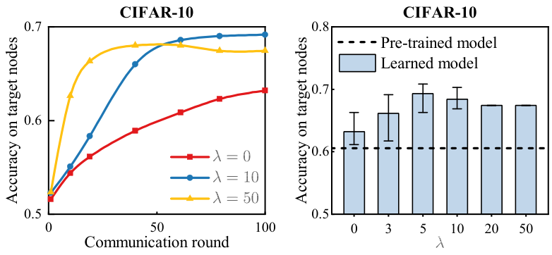
Figure 4. Impact of θp\theta_{p} and λ\lambda.

Impact of prior knowledge. To quantify the impact of the knowledge transfer on the convergence of model training and the adaptation performance of target nodes, we pre-train a prior model as θp\theta_{p} using images of 3-10 classes on CIFAR-10. Then, we train the meta-model θ\theta on source nodes with images of 1-8 classes and test the accuracy on the target nodes with all 1-10 classes. In this way, the pre-trained model can be considered as containing valuable knowledge of the current task. As shown in Figure 4, with the useful knowledge transferred from the previous task to the edge nodes, faster convergence, and higher adaptation performance are achieved by appropriately selecting the trade-off parameter λ\lambda. In other words, the regularization with useful knowledge transfer can help get a high-quality meta-model and achieve faster edge learning.

6. Conclusion

In this paper, we presented an inexact-ADMM based federated meta-learning approach for fast and continual edge learning. More specifically, we first proposed a platform-aided federated meta-learning architecture enabling edge nodes to collaboratively learn a meta-model with the knowledge transfer of previous tasks. We cast the federated meta-learning problem as a regularized optimization problem, where the previous knowledge is extracted as regularization. Then, we devised an ADMM based algorithm, namely ADMM-FedMeta, in which the original problem is decomposed into many subproblems which can be solved in parallel across edge nodes and the platform. Further, we developed a variant of the inexact-ADMM method to reduce the computational cost per round to 𝒪⁡(n)\mathcal{O}(n) via employing linear approximation as well as Hessian estimation. We provided a comprehensive analysis and empirical results to demonstrate the effectiveness and efficiency of ADMM-FedMeta. The advantages of the proposed algorithm are summarized as follows: First, it can decouple the regularizer from edge nodes to the platform, which helps to alleviate the local computational cost while exploiting the resources between local devices and the server effectively. Besides, by inexact-ADMM technique, we further reduce the computational complexity during local update and global aggregation. We show that ADMM-FedMeta can converge under mild conditions, particularly, with weak task similarity assumptions. Lastly, empirical results show that ADMM-FedMeta converges faster than existing benchmark algorithms.

There are a number of interesting questions and directions for future work. First, it is of interest to incorporate the experience replay method and parameter isolation approaches into the ADMM-FedMeta to further mitigate the catastrophic forgetting. Secondly, despite ADMM-FedMeta can be directly applied to reinforcement learning with policy gradient, it may lead to poor sample efficiency. It remains largely open to develop efficient collaborative reinforcement learning for edge learning. Moreover, our experimental results indicate that even without the regularization term, in practice ADMM-FedMeta can still converge faster than the existing gradient-based methods, especially on small sample sizes. It is intriguing to get a more deep understanding of this phenomenon.

7. Acknowledgments

This research was supported in part by NSF under Grants CNS-2003081 and CPS-1739344, National Key R&D Program of China under Grant No. 2019YFA0706403, National Natural Science Foundation of China under Grants No. 62072472, 61702562 and U19A2067, Natural Science Foundation of Hunan Province, China under Grant No. 2020JJ2050, 111 Project under Grant No. B18059, the Young Elite Scientists Sponsorship Program by CAST under Grant No. 2018QNRC001, the Young Talents Plan of Hunan Province of China under Grant No. 2019RS2001, and also financially supported by China Scholarship Council (CSC).

References

  • (1)
  • Barber and Sidky (2020) Rina Foygel Barber and Emil Y Sidky. 2020. Convergence for nonconvex ADMM, with applications to CT imaging. arXiv preprint arXiv:2006.07278 (2020).
  • Barros et al. (2018) Pablo Barros, German I Parisi, Di Fu, Xun Liu, and Stefan Wermter. 2018. Expectation learning for adaptive crossmodal stimuli association. arXiv preprint arXiv:1801.07654 (2018).
  • Boyd et al. (2011) Stephen Boyd, Neal Parikh, and Eric Chu. 2011. Distributed optimization and statistical learning via the alternating direction method of multipliers. Now Publishers Inc.
  • Bregman (1967) Lev M Bregman. 1967. The relaxation method of finding the common point of convex sets and its application to the solution of problems in convex programming. USSR computational mathematics and mathematical physics 7, 3 (1967), 200–217.
  • Chen et al. (2018) Fei Chen, Mi Luo, Zhenhua Dong, Zhenguo Li, and Xiuqiang He. 2018. Federated meta-learning with fast convergence and efficient communication. arXiv preprint arXiv:1802.07876 (2018).
  • Collins et al. (2020) Liam Collins, Aryan Mokhtari, and Sanjay Shakkottai. 2020. Distribution-Agnostic Model-Agnostic Meta-Learning. arXiv preprint arXiv:2002.04766 (2020).
  • Fallah et al. (2020a) Alireza Fallah, Aryan Mokhtari, and Asuman Ozdaglar. 2020a. On the convergence theory of gradient-based model-agnostic meta-learning algorithms. In International Conference on Artificial Intelligence and Statistics. 1082–1092.
  • Fallah et al. (2020b) Alireza Fallah, Aryan Mokhtari, and Asuman Ozdaglar. 2020b. Personalized federated learning: A meta-learning approach. arXiv preprint arXiv:2002.07948 (2020).
  • Finn et al. (2017) Chelsea Finn, Pieter Abbeel, and Sergey Levine. 2017. Model-agnostic meta-learning for fast adaptation of deep networks. arXiv preprint arXiv:1703.03400 (2017).
  • Finn et al. (2018) Chelsea Finn, Kelvin Xu, and Sergey Levine. 2018. Probabilistic model-agnostic meta-learning. In Advances in Neural Information Processing Systems. 9516–9527.
  • French (1999) Robert M French. 1999. Catastrophic forgetting in connectionist networks. Trends in cognitive sciences 3, 4 (1999), 128–135.
  • Hong et al. (2016) Mingyi Hong, Zhi-Quan Luo, and Meisam Razaviyayn. 2016. Convergence analysis of alternating direction method of multipliers for a family of nonconvex problems. SIAM Journal on Optimization 26, 1 (2016), 337–364.
  • Ji et al. (2020) Kaiyi Ji, Junjie Yang, and Yingbin Liang. 2020. Multi-Step Model-Agnostic Meta-Learning: Convergence and Improved Algorithms. arXiv preprint arXiv:2002.07836 (2020).
  • Jiang et al. (2019b) Bo Jiang, Tianyi Lin, Shiqian Ma, and Shuzhong Zhang. 2019b. Structured nonconvex and nonsmooth optimization: algorithms and iteration complexity analysis. Computational Optimization and Applications 72, 1 (2019), 115–157.
  • Jiang et al. (2019a) Yihan Jiang, Jakub Konečnỳ, Keith Rush, and Sreeram Kannan. 2019a. Improving federated learning personalization via model agnostic meta learning. arXiv preprint arXiv:1909.12488 (2019).
  • Jung et al. (2016) Heechul Jung, Jeongwoo Ju, Minju Jung, and Junmo Kim. 2016. Less-forgetting learning in deep neural networks. arXiv preprint arXiv:1607.00122 (2016).
  • Kirkpatrick et al. (2017) James Kirkpatrick, Razvan Pascanu, Neil Rabinowitz, Joel Veness, Guillaume Desjardins, Andrei A Rusu, Kieran Milan, John Quan, Tiago Ramalho, Agnieszka Grabska-Barwinska, et al. 2017. Overcoming catastrophic forgetting in neural networks. Proceedings of the national academy of sciences 114, 13 (2017), 3521–3526.
  • Krishnan and Balaprakash (2020) R Krishnan and Prasanna Balaprakash. 2020. Meta Continual Learning via Dynamic Programming. arXiv preprint arXiv:2008.02219 (2020).
  • Krizhevsky et al. (2009) Alex Krizhevsky, Geoffrey Hinton, et al. 2009. Learning multiple layers of features from tiny images. (2009).
  • Lanza et al. (2017) Alessandro Lanza, Serena Morigi, Ivan Selesnick, and Fiorella Sgallari. 2017. Nonconvex nonsmooth optimization via convex–nonconvex majorization–minimization. Numer. Math. 136, 2 (2017), 343–381.
  • Lin et al. (2020) Sen Lin, Guang Yang, and Junshan Zhang. 2020. A Collaborative Learning Framework via Federated Meta-Learning. arXiv preprint arXiv:2001.03229 (2020).
  • Lopez-Paz and Ranzato (2017) David Lopez-Paz and Marc’Aurelio Ranzato. 2017. Gradient episodic memory for continual learning. In Advances in neural information processing systems. 6467–6476.
  • Magnússon et al. (2015) Sindri Magnússon, Pradeep Chathuranga Weeraddana, Michael G Rabbat, and Carlo Fischione. 2015. On the convergence of alternating direction lagrangian methods for nonconvex structured optimization problems. IEEE Transactions on Control of Network Systems 3, 3 (2015), 296–309.
  • McMahan et al. (2017) Brendan McMahan, Eider Moore, Daniel Ramage, Seth Hampson, and Blaise Aguera y Arcas. 2017. Communication-efficient learning of deep networks from decentralized data. In Artificial Intelligence and Statistics. 1273–1282.
  • Mukkamala et al. (2020) Mahesh Chandra Mukkamala, Peter Ochs, Thomas Pock, and Shoham Sabach. 2020. Convex-Concave Backtracking for Inertial Bregman Proximal Gradient Algorithms in Nonconvex Optimization. SIAM Journal on Mathematics of Data Science 2, 3 (2020), 658–682.
  • Nichol et al. (2018) Alex Nichol, Joshua Achiam, and John Schulman. 2018. On first-order meta-learning algorithms. arXiv preprint arXiv:1803.02999 (2018).
  • Parisi et al. (2019) German I Parisi, Ronald Kemker, Jose L Part, Christopher Kanan, and Stefan Wermter. 2019. Continual lifelong learning with neural networks: A review. Neural Networks 113 (2019), 54–71.
  • Park et al. (2019) Jihong Park, Sumudu Samarakoon, Mehdi Bennis, and Mérouane Debbah. 2019. Wireless network intelligence at the edge. Proc. IEEE 107, 11 (2019), 2204–2239.
  • Raghu et al. (2019) Aniruddh Raghu, Maithra Raghu, Samy Bengio, and Oriol Vinyals. 2019. Rapid learning or feature reuse? towards understanding the effectiveness of maml. arXiv preprint arXiv:1909.09157 (2019).
  • Ravi and Larochelle (2016) Sachin Ravi and Hugo Larochelle. 2016. Optimization as a model for few-shot learning. (2016).
  • Schwarz et al. (2018) Jonathan Schwarz, Jelena Luketina, Wojciech M Czarnecki, Agnieszka Grabska-Barwinska, Yee Whye Teh, Razvan Pascanu, and Raia Hadsell. 2018. Progress & compress: A scalable framework for continual learning. arXiv preprint arXiv:1805.06370 (2018).
  • Si et al. (2009) Si Si, Dacheng Tao, and Bo Geng. 2009. Bregman divergence-based regularization for transfer subspace learning. IEEE Transactions on Knowledge and Data Engineering 22, 7 (2009), 929–942.
  • Song et al. (2019) Xingyou Song, Wenbo Gao, Yuxiang Yang, Krzysztof Choromanski, Aldo Pacchiano, and Yunhao Tang. 2019. Es-maml: Simple hessian-free meta learning. arXiv preprint arXiv:1910.01215 (2019).
  • Takada and Fujisawa (2020) Masaaki Takada and Hironori Fujisawa. 2020. Transfer Learning via ℓ1\ell_{1} Regularization. Advances in Neural Information Processing Systems 33 (2020).
  • Wang et al. (2018) Fenghui Wang, Wenfei Cao, and Zongben Xu. 2018. Convergence of multi-block Bregman ADMM for nonconvex composite problems. Science China Information Sciences 61, 12 (2018), 122101.
  • Wang et al. (2014) Fenghui Wang, Zongben Xu, and Hong-Kun Xu. 2014. Convergence of Bregman alternating direction method with multipliers for nonconvex composite problems. arXiv preprint arXiv:1410.8625 (2014).
  • Wang et al. (2019b) Junxiang Wang, Fuxun Yu, Xiang Chen, and Liang Zhao. 2019b. Admm for efficient deep learning with global convergence. In Proceedings of the 25th ACM SIGKDD International Conference on Knowledge Discovery & Data Mining. 111–119.
  • Wang et al. (2020) Lingxiao Wang, Qi Cai, Zhuoran Yang, and Zhaoran Wang. 2020. On the Global Optimality of Model-Agnostic Meta-Learning. arXiv preprint arXiv:2006.13182 (2020).
  • Wang et al. (2019a) Yu Wang, Wotao Yin, and Jinshan Zeng. 2019a. Global convergence of ADMM in nonconvex nonsmooth optimization. Journal of Scientific Computing 78, 1 (2019), 29–63.
  • Wu et al. (2020) Qiong Wu, Kaiwen He, and Xu Chen. 2020. Personalized federated learning for intelligent iot applications: A cloud-edge based framework. IEEE Computer Graphics and Applications (2020).
  • Xiao et al. (2017) Han Xiao, Kashif Rasul, and Roland Vollgraf. 2017. Fashion-mnist: a novel image dataset for benchmarking machine learning algorithms. arXiv preprint arXiv:1708.07747 (2017).
  • Yu et al. (2013) Dong Yu, Kaisheng Yao, Hang Su, Gang Li, and Frank Seide. 2013. KL-divergence regularized deep neural network adaptation for improved large vocabulary speech recognition. In 2013 IEEE International Conference on Acoustics, Speech and Signal Processing. IEEE, 7893–7897.
  • Yue et al. (2020) Sheng Yue, Ju Ren, Jiang Xin, Sen Lin, and Junshan Zhang. 2020. Inexact-ADMM based Federated Meta-Learning for Fast and Continual Edge Learning. arXiv:2012.08677 [cs.LG]
  • Zenke et al. (2017) Friedemann Zenke, Ben Poole, and Surya Ganguli. 2017. Continual learning through synaptic intelligence. Proceedings of machine learning research 70 (2017), 3987.
  • Zhang et al. (2020a) Xinwei Zhang, Mingyi Hong, Sairaj Dhople, Wotao Yin, and Yang Liu. 2020a. FedPD: A Federated Learning Framework with Optimal Rates and Adaptivity to Non-IID Data. arXiv preprint arXiv:2005.11418 (2020).
  • Zhang et al. (2020b) Zhaofeng Zhang, Sen Lin, Mehmet Dedeoglu, Kemi Ding, and Junshan Zhang. 2020b. Data-driven Distributionally Robust Optimization for Edge Intelligence. In IEEE INFOCOM 2020-IEEE Conference on Computer Communications. IEEE, 2619–2628.
  • Zheng et al. (2020) Wenbo Zheng, Lan Yan, Chao Gou, and Fei-Yue Wang. 2020. Federated Meta-Learning for Fraudulent Credit Card Detection. Proceedings of the Twenty-Ninth International Joint Conference on Artificial Intelligence (IJCAI-20) (2020).
  • Zhou et al. (2019) Zhi Zhou, Xu Chen, En Li, Liekang Zeng, Ke Luo, and Junshan Zhang. 2019. Edge intelligence: Paving the last mile of artificial intelligence with edge computing. Proc. IEEE 107, 8 (2019), 1738–1762.

Appendix

Appendix A Proof of Lemma 2

The proof is standard. For simplicity, we denote Fi(θ)≜Li(θ−α∇Li(θ,𝒟is),𝒟iq)F_{i}(\theta)\triangleq L_{i}\big(\theta-\alpha\nabla L_{i}(\theta,\mathcal{D}^{s}_{i}),\mathcal{D}^{q}_{i}\big). Recall that ∇Fi(x)=(In−α∇2Li(x,𝒟is))∇Li(x−α∇Li(x,𝒟is),𝒟iq)\nabla F_{i}(x)=\big(I_{n}-\alpha\nabla^{2}L_{i}(x,\mathcal{D}^{s}_{i})\big)\nabla L_{i}\big(x-\alpha\nabla L_{i}(x,\mathcal{D}^{s}_{i}),\mathcal{D}^{q}_{i}\big), and we have

(36) ‖∇Fi​(x)−∇Fi​(y)‖≤\displaystyle\big\|\nabla F_{i}(x)-\nabla F_{i}(y)\big\|\leq ∥∇Li(x−α∇Li(x,𝒟is),𝒟iq)−∇Li(y−α∇Li(y,𝒟is),𝒟iq)∥\displaystyle\big\|\nabla L_{i}\big(x-\alpha\nabla L_{i}(x,\mathcal{D}^{s}_{i}),\mathcal{D}^{q}_{i}\big)-\nabla L_{i}\big(y-\alpha\nabla L_{i}(y,\mathcal{D}^{s}_{i}),\mathcal{D}^{q}_{i}\big)\big\|
+α∥∇2Li(x,𝒟is)∇Li(x−α∇Li(x,𝒟is),𝒟iq)\displaystyle+\alpha\big\|\nabla^{2}L_{i}(x,\mathcal{D}^{s}_{i})\nabla L_{i}\big(x-\alpha\nabla L_{i}(x,\mathcal{D}^{s}_{i}),\mathcal{D}^{q}_{i}\big)
(37) −∇2Li(y,𝒟is)∇Li(y−α∇Li(y,𝒟is),𝒟iq)∥,\displaystyle-\nabla^{2}L_{i}(y,\mathcal{D}^{s}_{i})\nabla L_{i}\big(y-\alpha\nabla L_{i}(y,\mathcal{D}^{s}_{i}),\mathcal{D}^{q}_{i}\big)\big\|,

and

(38) −μi​In⪯∇2Li​(x,𝒟is)⪯μi​In,∀x∈ℝn.\displaystyle-\mu_{i}I_{n}\preceq\nabla^{2}L_{i}(x,\mathcal{D}^{s}_{i})\preceq\mu_{i}I_{n},~\forall x\in\mathbb{R}^{n}.

To prove (22), we need to bound (36) and (37). For (36), based on Assumption 2, we have

∥∇Li(x−α∇Li(x,𝒟is),𝒟iq)−∇Li(y−α∇Li(y,𝒟is),𝒟iq)∥\displaystyle\big\|\nabla L_{i}\big(x-\alpha\nabla L_{i}(x,\mathcal{D}^{s}_{i}),\mathcal{D}^{q}_{i}\big)-\nabla L_{i}\big(y-\alpha\nabla L_{i}(y,\mathcal{D}^{s}_{i}),\mathcal{D}^{q}_{i}\big)\big\|
≤\displaystyle\leq μi​‖x−y−α⁡(∇Li​(x,𝒟is)−∇Li​(y,𝒟is))‖\displaystyle\mu_{i}\big\|x-y-\alpha\big(\nabla L_{i}(x,\mathcal{D}^{s}_{i})-\nabla L_{i}(y,\mathcal{D}^{s}_{i})\big)\big\|
≤\displaystyle\leq μi​(‖x−y‖+α​‖∇Li​(x,𝒟is)−∇Li​(y,𝒟is)‖)\displaystyle\mu_{i}\big(\|x-y\|+\alpha\|\nabla L_{i}(x,\mathcal{D}^{s}_{i})-\nabla L_{i}(y,\mathcal{D}^{s}_{i})\|\big)
(39) ≤\displaystyle\leq (1+α​μi)​μi​‖x−y‖.\displaystyle(1+\alpha\mu_{i})\mu_{i}\|x-y\|.

To bound (37), it can be shown that

∥∇2Li(x,𝒟is)∇Li(x−α∇Li(x,𝒟is),𝒟iq)−∇2Li(y,𝒟is)∇Li(y−α∇Li(y,𝒟is),𝒟iq)∥\displaystyle\big\|\nabla^{2}L_{i}(x,\mathcal{D}^{s}_{i})\nabla L_{i}\big(x-\alpha\nabla L_{i}(x,\mathcal{D}^{s}_{i}),\mathcal{D}^{q}_{i}\big)-\nabla^{2}L_{i}(y,\mathcal{D}^{s}_{i})\nabla L_{i}\big(y-\alpha\nabla L_{i}(y,\mathcal{D}^{s}_{i}),\mathcal{D}^{q}_{i}\big)\big\|
=\displaystyle= ∥∇2Li(x,𝒟is)∇Li(x−α∇Li(x,𝒟is),𝒟iq)−∇2Li(x,𝒟is)∇Li(y−α∇Li(y,𝒟is),𝒟iq)\displaystyle\big\|\nabla^{2}L_{i}(x,\mathcal{D}^{s}_{i})\nabla L_{i}\big(x-\alpha\nabla L_{i}(x,\mathcal{D}^{s}_{i}),\mathcal{D}^{q}_{i}\big)-\nabla^{2}L_{i}(x,\mathcal{D}^{s}_{i})\nabla L_{i}\big(y-\alpha\nabla L_{i}(y,\mathcal{D}^{s}_{i}),\mathcal{D}^{q}_{i}\big)
+∇2Li(x,𝒟is)∇Li(y−α∇Li(y,𝒟is),𝒟iq)−∇2Li(y,𝒟is)∇Li(y−α∇Li(y,𝒟is),𝒟iq)∥\displaystyle+\nabla^{2}L_{i}(x,\mathcal{D}^{s}_{i})\nabla L_{i}\big(y-\alpha\nabla L_{i}(y,\mathcal{D}^{s}_{i}),\mathcal{D}^{q}_{i}\big)-\nabla^{2}L_{i}(y,\mathcal{D}^{s}_{i})\nabla L_{i}\big(y-\alpha\nabla L_{i}(y,\mathcal{D}^{s}_{i}),\mathcal{D}^{q}_{i}\big)\big\|
≤\displaystyle\leq ∥∇2Li(x,𝒟is)∥⋅∥∇Li(x−α∇Li(x,𝒟is),𝒟iq)−∇Li(y−α∇Li(y,𝒟is),𝒟iq)∥\displaystyle\big\|\nabla^{2}L_{i}(x,\mathcal{D}^{s}_{i})\big\|\cdot\big\|\nabla L_{i}\big(x-\alpha\nabla L_{i}(x,\mathcal{D}^{s}_{i}),\mathcal{D}^{q}_{i}\big)-\nabla L_{i}\big(y-\alpha\nabla L_{i}(y,\mathcal{D}^{s}_{i}),\mathcal{D}^{q}_{i}\big)\big\|
+∥∇2Li(x,𝒟is)−∇2Li(y,𝒟is)∥⋅∥∇Li(y−α∇Li(y,𝒟is),𝒟iq)∥\displaystyle+\big\|\nabla^{2}L_{i}(x,\mathcal{D}^{s}_{i})-\nabla^{2}L_{i}(y,\mathcal{D}^{s}_{i})\big\|\cdot\big\|\nabla L_{i}\big(y-\alpha\nabla L_{i}(y,\mathcal{D}^{s}_{i}),\mathcal{D}^{q}_{i}\big)\big\|
≤\displaystyle\leq ((1+αμi)μi2+ζi∥∇Li(y−α∇Li(y,𝒟is),𝒟iq)∥)∥x−y∥\displaystyle\Big((1+\alpha\mu_{i})\mu^{2}_{i}+\zeta_{i}\big\|\nabla L_{i}\big(y-\alpha\nabla L_{i}(y,\mathcal{D}^{s}_{i}),\mathcal{D}^{q}_{i}\big)\big\|\Big)\|x-y\|
(40) ≤\displaystyle\leq ((1+α​μi)​μi2+ζi​βi)​‖x−y‖,\displaystyle\big((1+\alpha\mu_{i})\mu^{2}_{i}+\zeta_{i}\beta_{i}\big)\|x-y\|,

where (A) follows from (18), (38), (A) and Assumption 3. Combining (A) and (A) yields the result.

Appendix B Proof of Lemma 1

Based on Lemma 2, we next prove the Lemmas 1-1 for the convergence analysis. In the following lemma, we first bound the variations of yity^{t}_{i} via the variations of θt\theta^{t}. For simplicity, denote

(41) fi(θ)≜Li(θ,𝒟is),fiq(ϕi)≜Li(ϕi,𝒟iq),Fi(θ)≜Li(θ−α∇Li(θ,𝒟is),𝒟iq).\displaystyle f_{i}(\theta)\triangleq L_{i}(\theta,\mathcal{D}^{s}_{i}),~f^{q}_{i}(\phi_{i})\triangleq L_{i}(\phi_{i},\mathcal{D}^{q}_{i}),~F_{i}(\theta)\triangleq L_{i}\big(\theta-\alpha\nabla L_{i}(\theta,\mathcal{D}^{s}_{i}),\mathcal{D}^{q}_{i}\big).
Lemma 0.

Suppose that Assumption 1-3 are satisfied. Then, the following holds true

(42) ‖yit+1−yit‖≤wi​νi​‖θt+1−θt‖+(δi,t+δi,t+1)​α​wi​ζi​βi2.\displaystyle\|y^{t+1}_{i}-y^{t}_{i}\|\leq w_{i}\nu_{i}\|\theta^{t+1}-\theta^{t}\|+(\delta_{i,t}+\delta_{i,t+1})\alpha w_{i}\zeta_{i}\beta^{2}_{i}.
Proof.

First, define

(43) ∇~​Fi​(θt+1)≜∇fiq​(ϕit+1)−α​git+1,\displaystyle\tilde{\nabla}F_{i}(\theta^{t+1})\triangleq\nabla f^{q}_{i}(\phi^{t+1}_{i})-\alpha g^{t+1}_{i},

where ϕit+1=θt+1−α∇fi(θt+1)\phi^{t+1}_{i}=\theta^{t+1}-\alpha\nabla f_{i}(\theta^{t+1}). We have the following observation from (12)

(44) wi​∇~​Fi​(θt+1)+yit+ρi​(θit+1−θt+1)=0.\displaystyle w_{i}\tilde{\nabla}F_{i}(\theta^{t+1})+y^{t}_{i}+\rho_{i}(\theta^{t+1}_{i}-\theta^{t+1})=0.

Using (13), we conclude that (44) is equivalent to

(45) −yit+1=wi​∇~​Fi​(θt+1).\displaystyle-y^{t+1}_{i}=w_{i}\tilde{\nabla}F_{i}(\theta^{t+1}).

Thus, for all t∈ℕt\in\mathbb{N}, the following is true

(46) ‖yit+1−yit‖=wi​‖∇~​Fi​(θt+1)−∇~​Fi​(θt)‖⏟(a).\displaystyle\|y^{t+1}_{i}-y^{t}_{i}\|=w_{i}\underbrace{\|\tilde{\nabla}F_{i}(\theta^{t+1})-\tilde{\nabla}F_{i}(\theta^{t})\|}_{\text{(a)}}.

Using Lemma 2, we derive the upper bound of (a) as follows

(a)=\displaystyle\text{(a)}= ‖(∇Fi​(θt+1)−∇~​Fi​(θt+1))−(∇Fi​(θt+1)−∇~​Fi​(θt))‖\displaystyle\big\|\big(\nabla F_{i}(\theta^{t+1})-\tilde{\nabla}F_{i}(\theta^{t+1})\big)-\big(\nabla F_{i}(\theta^{t+1})-\tilde{\nabla}F_{i}(\theta^{t})\big)\big\|
≤\displaystyle\leq ‖∇Fi​(θt+1)−∇~​Fi​(θt+1)‖+‖∇Fi​(θt+1)−∇~​Fi​(θt)‖\displaystyle\|\nabla F_{i}(\theta^{t+1})-\tilde{\nabla}F_{i}(\theta^{t+1})\|+\|\nabla F_{i}(\theta^{t+1})-\tilde{\nabla}F_{i}(\theta^{t})\|
≤\displaystyle\leq ‖∇Fi​(θt+1)−∇~​Fi​(θt+1)‖+‖∇Fi​(θt+1)−∇Fi​(θt)‖+‖∇Fi​(θt)−∇~​Fi​(θt)‖\displaystyle\|\nabla F_{i}(\theta^{t+1})-\tilde{\nabla}F_{i}(\theta^{t+1})\|+\|\nabla F_{i}(\theta^{t+1})-\nabla F_{i}(\theta^{t})\|+\|\nabla F_{i}(\theta^{t})-\tilde{\nabla}F_{i}(\theta^{t})\|
(47) ≤\displaystyle\leq νi​‖θt+1−θt‖+(δi,t+δi,t+1)​α​ζi​βi2,\displaystyle\nu_{i}\|\theta^{t+1}-\theta^{t}\|+(\delta_{i,t}+\delta_{i,t+1})\alpha\zeta_{i}\beta^{2}_{i},

where the last equality uses the following result in (Fallah et al. 2020a)

(48) ∥∇2fi(θt+1)∇fiq(ϕit+1)−git+1∥≤δi,t+1ζiβi2.\displaystyle\big\|\nabla^{2}f_{i}(\theta^{t+1})\nabla f^{q}_{i}(\phi^{t+1}_{i})-g^{t+1}_{i}\big\|\leq\delta_{i,t+1}\zeta_{i}\beta^{2}_{i}.

Plugging (B) into (46), we have

(49) ‖yit+1−yit‖≤\displaystyle\|y^{t+1}_{i}-y^{t}_{i}\|\leq wi​νi​‖θt+1−θt‖+(δi,t+δi,t+1)​α​wi​ζi​βi2,\displaystyle w_{i}\nu_{i}\|\theta^{t+1}-\theta^{t}\|+(\delta_{i,t}+\delta_{i,t+1})\alpha w_{i}\zeta_{i}\beta^{2}_{i},

which completes the proof. ∎

Appendix C Proof of Lemma 1

To bound the successive difference of the augmented Lagrangian function ℒ⁡({θit,yit},θt)\mathcal{L}\big(\{\theta^{t}_{i},y^{t}_{i}\},\theta^{t}\big) defined in (3.2), we first bound the successive difference of ℒi​(θi,θt+1,yit)\mathcal{L}_{i}(\theta_{i},\theta^{t+1},y^{t}_{i}), which is defined as follows

(50) ℒi​(θi,θt+1,yit)≜\displaystyle\mathcal{L}_{i}(\theta_{i},\theta^{t+1},y^{t}_{i})\triangleq wi​Fi​(θi)+⟨yit,θi−θt+1⟩+ρi2​‖θi−θt+1‖2.\displaystyle w_{i}F_{i}(\theta_{i})+\langle y^{t}_{i},\theta_{i}-\theta^{t+1}\rangle+\frac{\rho_{i}}{2}\|\theta_{i}-\theta^{t+1}\|^{2}.

Then, we have the following lemma.

Lemma 0.

Suppose that Assumption 1-3 are satisfied. The following holds true

ℒi​(θit+1,θt+1,yit)−ℒi​(θit,θt+1,yit)≤\displaystyle\mathcal{L}_{i}(\theta^{t+1}_{i},\theta^{t+1},y^{t}_{i})-\mathcal{L}_{i}(\theta^{t}_{i},\theta^{t+1},y^{t}_{i})\leq −ρi−(3+4​wi)​νi2​‖θit+1−θit‖2+2​(1+wi)​νiρi2​‖yit+1−yit‖2\displaystyle-\frac{\rho_{i}-(3+4w_{i})\nu_{i}}{2}\|\theta^{t+1}_{i}-\theta^{t}_{i}\|^{2}+\frac{2(1+w_{i})\nu_{i}}{\rho^{2}_{i}}\|y^{t+1}_{i}-y^{t}_{i}\|^{2}
+2​α​wi​ζi​βi2​δi,t+1ρi​‖yit+1−yit‖+α​wi​ζi​βi2​δi,t+1​‖θit−θit+1‖.\displaystyle+\frac{2\alpha w_{i}\zeta_{i}\beta^{2}_{i}\delta_{i,t+1}}{\rho_{i}}\|y^{t+1}_{i}-y^{t}_{i}\|+\alpha w_{i}\zeta_{i}\beta^{2}_{i}\delta_{i,t+1}\|\theta^{t}_{i}-\theta^{t+1}_{i}\|.
Proof.

First, we define ℒ^i​(θi,θt+1,yit)\hat{\mathcal{L}}_{i}(\theta_{i},\theta^{t+1},y^{t}_{i}) and ℒ~i​(θi,θt+1,yit)\tilde{\mathcal{L}}_{i}(\theta_{i},\theta^{t+1},y^{t}_{i}) as follows

(51) ℒ^i​(θi,θt+1,yit)≜\displaystyle\hat{\mathcal{L}}_{i}(\theta_{i},\theta^{t+1},y^{t}_{i})\triangleq wi⟨(I−α∇2fi(θt+1))∇fiq(ϕit+1),θi−θt+1⟩+wiFi(θt+1)+⟨yit,θi−θt+1⟩\displaystyle w_{i}\big\langle\big(I-\alpha\nabla^{2}f_{i}(\theta^{t+1})\big)\nabla f^{q}_{i}(\phi^{t+1}_{i}),\theta_{i}-\theta^{t+1}\big\rangle+w_{i}F_{i}(\theta^{t+1})+\langle y^{t}_{i},\theta_{i}-\theta^{t+1}\rangle
(52) +ρi2​‖θi−θt+1‖2,\displaystyle+\frac{\rho_{i}}{2}\|\theta_{i}-\theta^{t+1}\|^{2},
(53) ℒ~i​(θi,θt+1,yit)≜\displaystyle\tilde{\mathcal{L}}_{i}(\theta_{i},\theta^{t+1},y^{t}_{i})\triangleq wi​⟨∇fiq​(ϕit+1)−α​git+1,θi−θt+1⟩+wi​Fi​(θt+1)+⟨yit,θi−θt+1⟩\displaystyle w_{i}\big\langle\nabla f^{q}_{i}(\phi^{t+1}_{i})-\alpha g^{t+1}_{i},\theta_{i}-\theta^{t+1}\big\rangle+w_{i}F_{i}(\theta^{t+1})+\langle y^{t}_{i},\theta_{i}-\theta^{t+1}\rangle
(54) +ρi2​‖θi−θt+1‖2,\displaystyle+\frac{\rho_{i}}{2}\|\theta_{i}-\theta^{t+1}\|^{2},

where git+1g^{t+1}_{i} and ϕit+1\phi^{t+1}_{i} are defined in (11) and (8), respectively. For each i∈ℐi\in\mathcal{I}, using Lemma 2 yields

(55) ℒi​(θi,θt+1,yit)≤ℒ^i​(θi,θt+1,yit)+wi​νi2​‖θi−θt+1‖2.\displaystyle\mathcal{L}_{i}(\theta_{i},\theta^{t+1},y^{t}_{i})\leq\hat{\mathcal{L}}_{i}(\theta_{i},\theta^{t+1},y^{t}_{i})+\frac{w_{i}\nu_{i}}{2}\|\theta_{i}-\theta^{t+1}\|^{2}.

Recall that

(56) ∥∇2fi(θt+1)∇fiq(ϕit+1)−git+1∥≤ζiβi2δi,t+1.\displaystyle\|\nabla^{2}f_{i}(\theta^{t+1})\nabla f^{q}_{i}(\phi^{t+1}_{i})-g^{t+1}_{i}\|\leq\zeta_{i}\beta^{2}_{i}\delta_{i,t+1}.

Thus, using the Cauchy-Schwarz inequality, we can write

(57) ℒ^i​(θi,θt+1,yit)≤\displaystyle\hat{\mathcal{L}}_{i}(\theta_{i},\theta^{t+1},y^{t}_{i})\leq ℒ~i​(θi,θt+1,yit)+α​wi​ζi​βi2​δi,t+1​‖θi−θt+1‖.\displaystyle\tilde{\mathcal{L}}_{i}(\theta_{i},\theta^{t+1},y^{t}_{i})+\alpha w_{i}\zeta_{i}\beta^{2}_{i}\delta_{i,t+1}\|\theta_{i}-\theta^{t+1}\|.

Combining (55) and (57) yields that

(58) ℒi​(θi,θt+1,yit)≤\displaystyle\mathcal{L}_{i}(\theta_{i},\theta^{t+1},y^{t}_{i})\leq ℒ~i​(θi,θt+1,yit)+wi​νi2​‖θi−θt+1‖2+α​wi​ζi​βi2​δi,t+1​‖θi−θt+1‖.\displaystyle\tilde{\mathcal{L}}_{i}(\theta_{i},\theta^{t+1},y^{t}_{i})+\frac{w_{i}\nu_{i}}{2}\|\theta_{i}-\theta^{t+1}\|^{2}+\alpha w_{i}\zeta_{i}\beta^{2}_{i}\delta_{i,t+1}\|\theta_{i}-\theta^{t+1}\|.

Based on (44) and the strong convexity of ℒ~i​(θi,θt+1,yit)\tilde{\mathcal{L}}_{i}(\theta_{i},\theta^{t+1},y^{t}_{i}) with modulus ρi\rho_{i}, we can show that for each i∈ℐi\in\mathcal{I}

(59) ℒ~i​(θit+1,θt+1,yit)−ℒ~i​(θit,θt+1,yit)≤−ρi2​‖θit+1−θit‖2.\displaystyle\tilde{\mathcal{L}}_{i}(\theta^{t+1}_{i},\theta^{t+1},y^{t}_{i})-\tilde{\mathcal{L}}_{i}(\theta^{t}_{i},\theta^{t+1},y^{t}_{i})\leq-\frac{\rho_{i}}{2}\|\theta^{t+1}_{i}-\theta^{t}_{i}\|^{2}.

It follows that

ℒ~i​(θit,θt+1,yit)−ℒi​(θit,θt+1,yit)\displaystyle\tilde{\mathcal{L}}_{i}(\theta^{t}_{i},\theta^{t+1},y^{t}_{i})-\mathcal{L}_{i}(\theta^{t}_{i},\theta^{t+1},y^{t}_{i})
=\displaystyle= wi​⟨∇fiq​(ϕit+1)−α​git+1,θit−θt+1⟩+wi​Fi​(θt+1)−wi​Fi​(θit)\displaystyle w_{i}\big\langle\nabla f^{q}_{i}(\phi^{t+1}_{i})-\alpha g^{t+1}_{i},\theta^{t}_{i}-\theta^{t+1}\big\rangle+w_{i}F_{i}(\theta^{t+1})-w_{i}F_{i}(\theta^{t}_{i})
=\displaystyle= wi​Fi​(θt+1)−wi​Fi​(θit)−wi​⟨∇Fi​(θit),θt+1−θit⟩−wi​νi2​‖θit−θt+1‖2+wi​νi2​‖θit−θt+1‖2\displaystyle w_{i}F_{i}(\theta^{t+1})-w_{i}F_{i}(\theta^{t}_{i})-w_{i}\langle\nabla F_{i}(\theta^{t}_{i}),\theta^{t+1}-\theta^{t}_{i}\rangle-\frac{w_{i}\nu_{i}}{2}\|\theta^{t}_{i}-\theta^{t+1}\|^{2}+\frac{w_{i}\nu_{i}}{2}\|\theta^{t}_{i}-\theta^{t+1}\|^{2}
+wi​⟨∇fiq​(ϕit+1)−α​git+1−∇Fi​(θit),θit−θt+1⟩\displaystyle+w_{i}\big\langle\nabla f^{q}_{i}(\phi^{t+1}_{i})-\alpha g^{t+1}_{i}-\nabla F_{i}(\theta^{t}_{i}),\theta^{t}_{i}-\theta^{t+1}\big\rangle
≤(a)\displaystyle\mathop{\leq}^{\text{(a)}} wi​⟨∇fiq​(ϕit+1)−α​git+1−∇Fi​(θit),θit−θt+1⟩+wi​νi2​‖θit−θt+1‖2\displaystyle w_{i}\big\langle\nabla f^{q}_{i}(\phi^{t+1}_{i})-\alpha g^{t+1}_{i}-\nabla F_{i}(\theta^{t}_{i}),\theta^{t}_{i}-\theta^{t+1}\big\rangle+\frac{w_{i}\nu_{i}}{2}\|\theta^{t}_{i}-\theta^{t+1}\|^{2}
≤\displaystyle\leq wi​‖∇fiq​(ϕit+1)−α​git+1−∇Fi​(θt+1)‖⋅‖θit−θt+1‖+wi​‖∇Fi​(θt+1)−∇Fi​(θit)‖⋅‖θit−θt+1‖+wi​νi2​‖θit−θt+1‖2\displaystyle w_{i}\|\nabla f^{q}_{i}(\phi^{t+1}_{i})-\alpha g^{t+1}_{i}-\nabla F_{i}(\theta^{t+1})\|\cdot\|\theta^{t}_{i}-\theta^{t+1}\|+w_{i}\|\nabla F_{i}(\theta^{t+1})-\nabla F_{i}(\theta^{t}_{i})\|\cdot\|\theta^{t}_{i}-\theta^{t+1}\|+\frac{w_{i}\nu_{i}}{2}\|\theta^{t}_{i}-\theta^{t+1}\|^{2}
≤\displaystyle\leq 3/2⋅wi​νi​‖θit−θt+1‖2+α​wi​ζi​βi2​δi,t+1​‖θit−θt+1‖\displaystyle 3/2\cdot w_{i}\nu_{i}\|\theta^{t}_{i}-\theta^{t+1}\|^{2}+\alpha w_{i}\zeta_{i}\beta^{2}_{i}\delta_{i,t+1}\|\theta^{t}_{i}-\theta^{t+1}\|
(60) ≤(b)\displaystyle\mathop{\leq}^{\text{(b)}} 3​wi​νi​(‖θit−θit+1‖2+‖θit+1−θt+1‖2)+α​wi​ζi​βi2​δi,t+1​(‖θit−θit+1‖+‖θit+1−θt+1‖),\displaystyle 3w_{i}\nu_{i}\big(\|\theta^{t}_{i}-\theta^{t+1}_{i}\|^{2}+\|\theta^{t+1}_{i}-\theta^{t+1}\|^{2}\big)+\alpha w_{i}\zeta_{i}\beta^{2}_{i}\delta_{i,t+1}\big(\|\theta^{t}_{i}-\theta^{t+1}_{i}\|+\|\theta^{t+1}_{i}-\theta^{t+1}\|\big),

where (a) is derived from Lemma 2 and (b) is based on the following fact

(61) ‖x+y‖2≤2​‖x‖2+2​‖y‖2,x,y∈ℝn.\displaystyle\|x+y\|^{2}\leq 2\|x\|^{2}+2\|y\|^{2},~x,y\in\mathbb{R}^{n}.

Combining (58)-(C), we conclude that

ℒi​(θit+1,θt+1,yit)−ℒi​(θit,θt+1,yit)\displaystyle\mathcal{L}_{i}(\theta^{t+1}_{i},\theta^{t+1},y^{t}_{i})-\mathcal{L}_{i}(\theta^{t}_{i},\theta^{t+1},y^{t}_{i})
≤\displaystyle\leq ℒ~i​(θit+1,θt+1,yit)−ℒ~i​(θit,θt+1,yit)+ℒ~i​(θit,θt+1,yit)−ℒi​(θit,θt+1,yit)\displaystyle\tilde{\mathcal{L}}_{i}(\theta^{t+1}_{i},\theta^{t+1},y^{t}_{i})-\tilde{\mathcal{L}}_{i}(\theta^{t}_{i},\theta^{t+1},y^{t}_{i})+\tilde{\mathcal{L}}_{i}(\theta^{t}_{i},\theta^{t+1},y^{t}_{i})-\mathcal{L}_{i}(\theta^{t}_{i},\theta^{t+1},y^{t}_{i})
+wi​νi2​‖θit−θt+1‖2+α​wi​ζi​βi2​δi,t+1​‖θit+1−θt+1‖\displaystyle+\frac{w_{i}\nu_{i}}{2}\|\theta^{t}_{i}-\theta^{t+1}\|^{2}+\alpha w_{i}\zeta_{i}\beta^{2}_{i}\delta_{i,t+1}\|\theta^{t+1}_{i}-\theta^{t+1}\|
≤\displaystyle\leq −ρi−8​wi​νi2​‖θit+1−θit‖2+4​wi​νi​‖θit+1−θt+1‖2+2​α​wi​ζi​βi2​δi,t+1​‖θit+1−θt+1‖\displaystyle-\frac{\rho_{i}-8w_{i}\nu_{i}}{2}\|\theta^{t+1}_{i}-\theta^{t}_{i}\|^{2}+4w_{i}\nu_{i}\|\theta^{t+1}_{i}-\theta^{t+1}\|^{2}+2\alpha w_{i}\zeta_{i}\beta^{2}_{i}\delta_{i,t+1}\|\theta^{t+1}_{i}-\theta^{t+1}\|
+α​wi​ζi​βi2​δi,t+1​‖θit−θit+1‖\displaystyle+\alpha w_{i}\zeta_{i}\beta^{2}_{i}\delta_{i,t+1}\|\theta^{t}_{i}-\theta^{t+1}_{i}\|
≤(c)\displaystyle\mathop{\leq}^{\text{(c)}} −ρi−8​wi​νi2​‖θit+1−θit‖2+4​wi​νiρi2​‖yit+1−yit‖2+2​α​wi​ζi​βi2​δi,t+1ρi​‖yit+1−yit‖\displaystyle-\frac{\rho_{i}-8w_{i}\nu_{i}}{2}\|\theta^{t+1}_{i}-\theta^{t}_{i}\|^{2}+\frac{4w_{i}\nu_{i}}{\rho^{2}_{i}}\|y^{t+1}_{i}-y^{t}_{i}\|^{2}+\frac{2\alpha w_{i}\zeta_{i}\beta^{2}_{i}\delta_{i,t+1}}{\rho_{i}}\|y^{t+1}_{i}-y^{t}_{i}\|
(62) +α​wi​ζi​βi2​δi,t+1​‖θit−θit+1‖,\displaystyle+\alpha w_{i}\zeta_{i}\beta^{2}_{i}\delta_{i,t+1}\|\theta^{t}_{i}-\theta^{t+1}_{i}\|,

where (c) is derived from (13). This completes the proof. ∎

Appendix D Proof of Lemma 1

Based on Lemma 1, we derive the successive difference of the augmented Lagrangian function ℒ⁡({θit,yit},θt)\mathcal{L}\big(\{\theta^{t}_{i},y^{t}_{i}\},\theta^{t}\big) in the following lemma. Note that due to the error induced by linear approximation and first-order Hessian estimation, the sufficient descent does not hold below.

Lemma 0.

Suppose that Assumption 1-3 hold. Then the following holds

ℒ⁡({θit+1,yit+1},θt+1)−ℒ⁡({θit,yit},θt)≤\displaystyle\mathcal{L}\big(\{\theta^{t+1}_{i},y^{t+1}_{i}\},\theta^{t+1}\big)-\mathcal{L}\big(\{\theta^{t}_{i},y^{t}_{i}\},\theta^{t}\big)\leq −∑i∈ℐ(ai,e∥θit+1−θit∥2+ai,p∥θt+1−θt∥2\displaystyle-\sum_{i\in\mathcal{I}}\Big(a_{i,e}\|\theta^{t+1}_{i}-\theta^{t}_{i}\|^{2}+a_{i,p}\|\theta^{t+1}-\theta^{t}\|^{2}
(63) OPEN−bi,et+1​‖θit+1−θit‖−bi,pt+1​‖θt+1−θt‖−cit+1),\displaystyle-b^{t+1}_{i,e}\|\theta^{t+1}_{i}-\theta^{t}_{i}\|-b^{t+1}_{i,p}\|\theta^{t+1}-\theta^{t}\|-c^{t+1}_{i}\Big),

where ai,ea_{i,e} and ai,pa_{i,p} are defined in (24) and (25), respectively. bi,et+1b^{t+1}_{i,e}, bi,et+1b^{t+1}_{i,e}, and cit+1c^{t+1}_{i} are defined as follows

(64) bi,et+1≜α​wi​ζi​βi2​δi,t+1,\displaystyle b^{t+1}_{i,e}\triangleq\alpha w_{i}\zeta_{i}\beta^{2}_{i}\delta_{i,t+1},
(65) bi,pt+1≜2​α​νi​wi2​ζi​βi2​δi,t+1ρi,\displaystyle b^{t+1}_{i,p}\triangleq\frac{2\alpha\nu_{i}w^{2}_{i}\zeta_{i}\beta^{2}_{i}\delta_{i,t+1}}{\rho_{i}},
(66) cit+1≜2​(δi,t+δi,t+1)2​(α​wi​ζi​βi2)2​(4​wi​νiρi2+1ρi)+2​(α​wi​ζi​βi2)2​δi,t+1ρi​(δi,t+δi,t+1).\displaystyle c^{t+1}_{i}\triangleq 2(\delta_{i,t}+\delta_{i,t+1})^{2}(\alpha w_{i}\zeta_{i}\beta^{2}_{i})^{2}\bigg(\frac{4w_{i}\nu_{i}}{\rho^{2}_{i}}+\frac{1}{\rho_{i}}\bigg)+\frac{2(\alpha w_{i}\zeta_{i}\beta^{2}_{i})^{2}\delta_{i,t+1}}{\rho_{i}}(\delta_{i,t}+\delta_{i,t+1}).
Proof.

Based on the update (13), we first obtain

ℒ⁡({θit+1,yit+1},θt+1)−ℒ⁡({θit+1,yit},θt+1)\displaystyle\mathcal{L}\big(\{\theta^{t+1}_{i},y^{t+1}_{i}\},\theta^{t+1}\big)-\mathcal{L}\big(\{\theta^{t+1}_{i},y^{t}_{i}\},\theta^{t+1}\big)
=\displaystyle= ∑i∈ℐ⟨yit+1−yit,θit+1−θt+1⟩\displaystyle\sum_{i\in\mathcal{I}}\langle y^{t+1}_{i}-y^{t}_{i},\theta^{t+1}_{i}-\theta^{t+1}\rangle
(67) =\displaystyle= ∑i∈ℐ1ρi​‖yit+1−yit‖2.\displaystyle\sum_{i\in\mathcal{I}}\frac{1}{\rho_{i}}\|y^{t+1}_{i}-y^{t}_{i}\|^{2}.

Using Lemma 1 and Assumption 2, we have

ℒ⁡({θit+1,yit},θt+1)−ℒ⁡({θit,yit},θt)\displaystyle\mathcal{L}\big(\{\theta^{t+1}_{i},y^{t}_{i}\},\theta^{t+1}\big)-\mathcal{L}\big(\{\theta^{t}_{i},y^{t}_{i}\},\theta^{t}\big)
=\displaystyle= ℒ⁡({θit+1,yit},θt+1)−ℒ⁡({θit,yit},θt+1)+ℒ⁡({θit,yit},θt+1)−ℒ⁡({θit,yit},θt)\displaystyle\mathcal{L}\big(\{\theta^{t+1}_{i},y^{t}_{i}\},\theta^{t+1}\big)-\mathcal{L}\big(\{\theta^{t}_{i},y^{t}_{i}\},\theta^{t+1}\big)+\mathcal{L}\big(\{\theta^{t}_{i},y^{t}_{i}\},\theta^{t+1}\big)-\mathcal{L}\big(\{\theta^{t}_{i},y^{t}_{i}\},\theta^{t}\big)
=\displaystyle= ∑i∈ℐ(ℒi​(θit+1,θt+1,yit)−ℒi​(θit,θt+1,yit))+ℒ⁡({θit,yit},θt+1)−ℒ⁡({θit,yit},θt)⏟(a)\displaystyle\sum_{i\in\mathcal{I}}\left(\mathcal{L}_{i}(\theta^{t+1}_{i},\theta^{t+1},y^{t}_{i})-\mathcal{L}_{i}(\theta^{t}_{i},\theta^{t+1},y^{t}_{i})\right)+\underbrace{\mathcal{L}\big(\{\theta^{t}_{i},y^{t}_{i}\},\theta^{t+1}\big)-\mathcal{L}\big(\{\theta^{t}_{i},y^{t}_{i}\},\theta^{t}\big)}_{\text{(a)}}
≤\displaystyle\leq −∑i∈ℐ(ρi−8​wi​νi2∥θit+1−θit∥2+ρi−λ​μr/I2∥θt+1−θt∥2−4​wi​νiρi2∥yit+1−yit∥2\displaystyle-\sum_{i\in\mathcal{I}}\bigg(\frac{\rho_{i}-8w_{i}\nu_{i}}{2}\|\theta^{t+1}_{i}-\theta^{t}_{i}\|^{2}+\frac{\rho_{i}-\lambda\mu_{r}/I}{2}\|\theta^{t+1}-\theta^{t}\|^{2}-\frac{4w_{i}\nu_{i}}{\rho^{2}_{i}}\|y^{t+1}_{i}-y^{t}_{i}\|^{2}
(68) OPEN−2​α​wi​ζi​βi2​δi,t+1ρi​‖yit+1−yit‖−α​wi​ζi​βi2​δi,t+1​‖θit+1−θit‖),\displaystyle-\frac{2\alpha w_{i}\zeta_{i}\beta^{2}_{i}\delta_{i,t+1}}{\rho_{i}}\|y^{t+1}_{i}-y^{t}_{i}\|-\alpha w_{i}\zeta_{i}\beta^{2}_{i}\delta_{i,t+1}\|\theta^{t+1}_{i}-\theta^{t}_{i}\|\bigg),

where the bound of (a) is derived in the similar way as in Lemma 1. Combining (D) and (D), we conclude that

ℒ⁡({θit+1,yit+1},θt+1)−ℒ⁡({θit,yit},θt)\displaystyle\mathcal{L}\big(\{\theta^{t+1}_{i},y^{t+1}_{i}\},\theta^{t+1}\big)-\mathcal{L}\big(\{\theta^{t}_{i},y^{t}_{i}\},\theta^{t}\big)
=\displaystyle= ℒ⁡({θit+1,yit+1},θt+1)−ℒ⁡({θit+1,yit}i,θt+1)+ℒ⁡({θit+1,yit},θt+1)−ℒ⁡({θit,yit},θt)\displaystyle\mathcal{L}\big(\{\theta^{t+1}_{i},y^{t+1}_{i}\},\theta^{t+1}\big)-\mathcal{L}\big(\{\theta^{t+1}_{i},y^{t}_{i}\}_{i},\theta^{t+1}\big)+\mathcal{L}\big(\{\theta^{t+1}_{i},y^{t}_{i}\},\theta^{t+1}\big)-\mathcal{L}\big(\{\theta^{t}_{i},y^{t}_{i}\},\theta^{t}\big)
=\displaystyle= −∑i∈ℐ[ρi−8​wi​νi2∥θit+1−θit∥2+ρi−λ​μr/I2∥θt+1−θt∥2−(4​wi​νiρi2+1ρi)∥yit+1−yit∥2\displaystyle-\sum_{i\in\mathcal{I}}\bigg[\frac{\rho_{i}-8w_{i}\nu_{i}}{2}\|\theta^{t+1}_{i}-\theta^{t}_{i}\|^{2}+\frac{\rho_{i}-\lambda\mu_{r}/I}{2}\|\theta^{t+1}-\theta^{t}\|^{2}-\Big(\frac{4w_{i}\nu_{i}}{\rho^{2}_{i}}+\frac{1}{\rho_{i}}\Big)\|y^{t+1}_{i}-y^{t}_{i}\|^{2}
−2​α​wi​ζi​βi2​δi,t+1ρi∥yit+1−yit∥−αwiζiβi2δi,t+1∥θit−θit+1∥]\displaystyle-\frac{2\alpha w_{i}\zeta_{i}\beta^{2}_{i}\delta_{i,t+1}}{\rho_{i}}\|y^{t+1}_{i}-y^{t}_{i}\|-\alpha w_{i}\zeta_{i}\beta^{2}_{i}\delta_{i,t+1}\|\theta^{t}_{i}-\theta^{t+1}_{i}\|\bigg]
≤\displaystyle\leq −∑i∈ℐ[ρi−8​wi​νi2∥θit+1−θit∥2+ρi−λ​μr/I2∥θt+1−θt∥2−(4​wi​νiρi2+1ρi)(2wi2νi2∥θt+1−θt∥2\displaystyle-\sum_{i\in\mathcal{I}}\bigg[\frac{\rho_{i}-8w_{i}\nu_{i}}{2}\|\theta^{t+1}_{i}-\theta^{t}_{i}\|^{2}+\frac{\rho_{i}-\lambda\mu_{r}/I}{2}\|\theta^{t+1}-\theta^{t}\|^{2}-\Big(\frac{4w_{i}\nu_{i}}{\rho^{2}_{i}}+\frac{1}{\rho_{i}}\Big)\Big(2w^{2}_{i}\nu^{2}_{i}\|\theta^{t+1}-\theta^{t}\|^{2}
OPEN+2​(δi,t+δi,t+1)2​(α​wi​ζi​βi2)2)−2​α​wi​ζi​βi2​δi,t+1ρi​(wi​νi​‖θt+1−θt‖+(δi,t+δi,t+1)​α​wi​ζi​βi2)−α​wi​ζi​βi2​δi,t+1​‖θit−θit+1‖\displaystyle+2(\delta_{i,t}+\delta_{i,t+1})^{2}(\alpha w_{i}\zeta_{i}\beta^{2}_{i})^{2}\Big)-\frac{2\alpha w_{i}\zeta_{i}\beta^{2}_{i}\delta_{i,t+1}}{\rho_{i}}\Big(w_{i}\nu_{i}\|\theta^{t+1}-\theta^{t}\|+(\delta_{i,t}+\delta_{i,t+1})\alpha w_{i}\zeta_{i}\beta^{2}_{i}\Big)-\alpha w_{i}\zeta_{i}\beta^{2}_{i}\delta_{i,t+1}\|\theta^{t}_{i}-\theta^{t+1}_{i}\|
(69) =\displaystyle= −∑i∈ℐ(ai,e∥θit+1−θit∥2+ai,p∥θt+1−θt∥2−bi,et+1∥θit+1−θit∥−bi,pt+1∥θt+1−θt∥−cit+1),\displaystyle-\sum_{i\in\mathcal{I}}\Big(a_{i,e}\|\theta^{t+1}_{i}-\theta^{t}_{i}\|^{2}+a_{i,p}\|\theta^{t+1}-\theta^{t}\|^{2}-b^{t+1}_{i,e}\|\theta^{t+1}_{i}-\theta^{t}_{i}\|-b^{t+1}_{i,p}\|\theta^{t+1}-\theta^{t}\|-c^{t+1}_{i}\Big),

thereby completing the proof. ∎

Appendix E Proof of Lemma 1

In the next lemma, we show that the augmented Lagrangian function ℒ⁡({θit,yit},θt)\mathcal{L}\big(\{\theta^{t}_{i},y^{t}_{i}\},\theta^{t}\big) is lower bounded for any t∈ℕt\in\mathbb{N}.

Lemma 0.

Given Assumption 1-5, the augmented Lagrangian function defined in (3.2) is lower bounded by Algorithm 1.

Proof.

Recall that in (45)

(70) −yit+1=wi​∇~​Fi​(θt+1),\displaystyle-y^{t+1}_{i}=w_{i}\tilde{\nabla}F_{i}(\theta^{t+1}),

where ∇~​Fi​(θt+1)=∇fiq​(ϕit+1)−α​git+1\tilde{\nabla}F_{i}(\theta^{t+1})=\nabla f^{q}_{i}(\phi^{t+1}_{i})-\alpha g^{t+1}_{i}. Besides, due to Lemma 2, we can write

Fi​(θt+1)≤\displaystyle F_{i}(\theta^{t+1})\leq Fi​(θit+1)+⟨∇Fi​(θit+1),θt+1−θit+1⟩+νi2​‖θit+1−θt+1‖2\displaystyle F_{i}(\theta^{t+1}_{i})+\langle\nabla F_{i}(\theta^{t+1}_{i}),\theta^{t+1}-\theta^{t+1}_{i}\rangle+\frac{\nu_{i}}{2}\|\theta^{t+1}_{i}-\theta^{t+1}\|^{2}
=\displaystyle= Fi​(θit+1)+⟨∇Fi​(θt+1),θt+1−θit+1⟩+⟨∇Fi​(θit+1)−∇Fi​(θt+1),θt+1−θit+1⟩+νi2​‖θit+1−θt+1‖2\displaystyle F_{i}(\theta^{t+1}_{i})+\langle\nabla F_{i}(\theta^{t+1}),\theta^{t+1}-\theta^{t+1}_{i}\rangle+\langle\nabla F_{i}(\theta^{t+1}_{i})-\nabla F_{i}(\theta^{t+1}),\theta^{t+1}-\theta^{t+1}_{i}\rangle+\frac{\nu_{i}}{2}\|\theta^{t+1}_{i}-\theta^{t+1}\|^{2}
(71) ≤\displaystyle\leq Fi​(θit+1)+⟨Fi​(θt+1),θt+1−θit+1⟩+3​νi2​‖θit+1−θt+1‖2.\displaystyle F_{i}(\theta^{t+1}_{i})+\langle F_{i}(\theta^{t+1}),\theta^{t+1}-\theta^{t+1}_{i}\rangle+\frac{3\nu_{i}}{2}\|\theta^{t+1}_{i}-\theta^{t+1}\|^{2}.

Based on the definition of the augmented Lagrangian function (3.2) and (E), we can show the following observation

ℒ⁡({θit+1,yit+1},θt+1)\displaystyle\mathcal{L}\big(\{\theta^{t+1}_{i},y^{t+1}_{i}\},\theta^{t+1}\big)
=\displaystyle= λ​Dh​(θt+1,θp)+∑i∈ℐ(wi​Fi​(θit+1)+⟨yit+1,θit+1−θt+1⟩+ρi2​‖θit+1−θt+1‖2)\displaystyle\lambda D_{h}(\theta^{t+1},\theta_{p})+\sum_{i\in\mathcal{I}}\Big(w_{i}F_{i}(\theta^{t+1}_{i})+\langle y^{t+1}_{i},\theta^{t+1}_{i}-\theta^{t+1}\rangle+\frac{\rho_{i}}{2}\|\theta^{t+1}_{i}-\theta^{t+1}\|^{2}\Big)
=\displaystyle= λ​Dh​(θt+1,θp)+∑i∈ℐ(wi​Fi​(θit+1)+⟨wi​∇~​Fi​(θt+1),θt+1−θit+1⟩+ρi2​‖θit+1−θt+1‖2)\displaystyle\lambda D_{h}(\theta^{t+1},\theta_{p})+\sum_{i\in\mathcal{I}}\Big(w_{i}F_{i}(\theta^{t+1}_{i})+\langle w_{i}\tilde{\nabla}F_{i}(\theta^{t+1}),\theta^{t+1}-\theta^{t+1}_{i}\rangle+\frac{\rho_{i}}{2}\|\theta^{t+1}_{i}-\theta^{t+1}\|^{2}\Big)
=\displaystyle= ∑i∈ℐ(wi​Fi​(θit+1)+⟨wi​∇~​Fi​(θt+1),θt+1−θit+1⟩+ρi2​‖θit+1−θt+1‖2)+λ​Dh​(θt+1,θp)\displaystyle\sum_{i\in\mathcal{I}}\Big(w_{i}F_{i}(\theta^{t+1}_{i})+\langle w_{i}\tilde{\nabla}F_{i}(\theta^{t+1}),\theta^{t+1}-\theta^{t+1}_{i}\rangle+\frac{\rho_{i}}{2}\|\theta^{t+1}_{i}-\theta^{t+1}\|^{2}\Big)+\lambda D_{h}(\theta^{t+1},\theta_{p})
=\displaystyle= ∑i∈ℐ(wiFi(θit+1)+⟨wi∇Fi(θt+1),θt+1−θit+1⟩+wi⟨∇~Fi(θt+1)−∇Fi(θt+1),θt+1−θit+1⟩\displaystyle\sum_{i\in\mathcal{I}}\Big(w_{i}F_{i}(\theta^{t+1}_{i})+\langle w_{i}\nabla F_{i}(\theta^{t+1}),\theta^{t+1}-\theta^{t+1}_{i}\rangle+w_{i}\langle\tilde{\nabla}F_{i}(\theta^{t+1})-\nabla F_{i}(\theta^{t+1}),\theta^{t+1}-\theta^{t+1}_{i}\rangle
OPEN+ρi2​‖θit+1−θt+1‖2)+λ​Dh​(θt+1,θp)\displaystyle+\frac{\rho_{i}}{2}\|\theta^{t+1}_{i}-\theta^{t+1}\|^{2}\Big)+\lambda D_{h}(\theta^{t+1},\theta_{p})
≥\displaystyle\geq ∑i∈ℐ(wiFi(θit+1)+⟨wi∇Fi(θt+1),θt+1−θit+1⟩−wi∥∇~Fi(θt+1)−∇Fi(θt+1)∥⋅∥θt+1−θit+1∥\displaystyle\sum_{i\in\mathcal{I}}\Big(w_{i}F_{i}(\theta^{t+1}_{i})+\langle w_{i}\nabla F_{i}(\theta^{t+1}),\theta^{t+1}-\theta^{t+1}_{i}\rangle-w_{i}\|\tilde{\nabla}F_{i}(\theta^{t+1})-\nabla F_{i}(\theta^{t+1})\|\cdot\|\theta^{t+1}-\theta^{t+1}_{i}\|
OPEN+ρi2​‖θit+1−θt+1‖2)+λ​Dh​(θt+1,θp)\displaystyle+\frac{\rho_{i}}{2}\|\theta^{t+1}_{i}-\theta^{t+1}\|^{2}\Big)+\lambda D_{h}(\theta^{t+1},\theta_{p})
≥\displaystyle\geq ∑i∈ℐ(wi​Fi​(θt+1)+ρi−3​νi2​‖θit+1−θt+1‖2−α​wi​ζi​βi2​δi,t+1​‖θt+1−θit+1‖)+λ​Dh​(θt+1,θp),\displaystyle\sum_{i\in\mathcal{I}}\Big(w_{i}F_{i}(\theta^{t+1})+\frac{\rho_{i}-3\nu_{i}}{2}\|\theta^{t+1}_{i}-\theta^{t+1}\|^{2}-\alpha w_{i}\zeta_{i}\beta^{2}_{i}\delta_{i,t+1}\|\theta^{t+1}-\theta^{t+1}_{i}\|\Big)+\lambda D_{h}(\theta^{t+1},\theta_{p}),

where the last inequality is derived from νi\nu_{i}-smoothness of FiF_{i} and first-order Taylor expansion. Due to Assumption 1, λ​Dh​(θt+1,θp)+∑i∈ℐwi​Fi​(θt+1)\lambda D_{h}(\theta^{t+1},\theta_{p})+\sum_{i\in\mathcal{I}}w_{i}F_{i}(\theta^{t+1}) is lower bounded. According to Assumption 5, it is easy to show that

(72) ∑i∈ℐ(CLOSE\displaystyle\sum_{i\in\mathcal{I}}\Big( OPENρi−3​νi2​‖θit+1−θt+1‖2−α​wi​ζi​βi2​δi,t+1​‖θt+1−θit+1‖)>−∞,\displaystyle\frac{\rho_{i}-3\nu_{i}}{2}\|\theta^{t+1}_{i}-\theta^{t+1}\|^{2}-\alpha w_{i}\zeta_{i}\beta^{2}_{i}\delta_{i,t+1}\|\theta^{t+1}-\theta^{t+1}_{i}\|\Big)>-\infty,

thereby completing the proof. ∎

Appendix F Proof of Theorem 3

First, we prove part (i). Note that the RHS of (1) is the sum of some independent quadratic functions of ‖θit+1−θit‖\|\theta^{t+1}_{i}-\theta^{t}_{i}\| and ‖θt+1−θt‖\|\theta^{t+1}-\theta^{t}\|. Due to Assumption 5 and Lemma 1, for each i∈ℐi\in\mathcal{I}, based on the form of roots of quadratic function, it is easy to see that there exist σit+1\sigma^{t+1}_{i} and γit+1\gamma^{t+1}_{i} such that

limt→∞σit+1=0,\displaystyle\lim_{t\rightarrow\infty}\sigma^{t+1}_{i}=0,
(73) limt→∞γit+1=0.\displaystyle\lim_{t\rightarrow\infty}\gamma^{t+1}_{i}=0.

When ‖θit+1−θit‖>σit+1\|\theta^{t+1}_{i}-\theta^{t}_{i}\|>\sigma^{t+1}_{i},

(74) ai,e​‖θit+1−θit‖2−bi,et+1​‖θit+1−θit‖−cit+1>0;\displaystyle a_{i,e}\|\theta^{t+1}_{i}-\theta^{t}_{i}\|^{2}-b^{t+1}_{i,e}\|\theta^{t+1}_{i}-\theta^{t}_{i}\|-c^{t+1}_{i}>0;

and when ‖θt+1−θt‖>γit+1\|\theta^{t+1}-\theta^{t}\|>\gamma^{t+1}_{i},

(75) ai,p​‖θt+1−θt‖2−bi,pt+1​‖θt+1−θt‖>0.\displaystyle a_{i,p}\|\theta^{t+1}-\theta^{t}\|^{2}-b^{t+1}_{i,p}\|\theta^{t+1}-\theta^{t}\|>0.

Next, we show limt→∞‖θit+1−θit‖=0\lim_{t\rightarrow\infty}\|\theta^{t+1}_{i}-\theta^{t}_{i}\|=0 and limt→∞‖θt+1−θt‖=0\lim_{t\rightarrow\infty}\|\theta^{t+1}-\theta^{t}\|=0 by two steps.

  1. 1)

    Suppose that there exists T≥0T\geq 0 such that for all t≥Tt\geq T, the following is true

    (76) ∑i∈ℐ(CLOSE\displaystyle\sum_{i\in\mathcal{I}}\Big( OPENai,e​‖θit+1−θit‖2+ai,p​‖θt+1−θt‖2−bi,et+1​‖θit+1−θit‖−bi,pt+1​‖θt+1−θt‖−cit+1)>0.\displaystyle a_{i,e}\|\theta^{t+1}_{i}-\theta^{t}_{i}\|^{2}+a_{i,p}\|\theta^{t+1}-\theta^{t}\|^{2}-b^{t+1}_{i,e}\|\theta^{t+1}_{i}-\theta^{t}_{i}\|-b^{t+1}_{i,p}\|\theta^{t+1}-\theta^{t}\|-c^{t+1}_{i}\Big)>0.

    It follows that under Assumption 5, using Lemma 1-1, ℒ⁡({θit+1,yit+1},θt+1)\mathcal{L}\big(\{\theta^{t+1}_{i},y^{t+1}_{i}\},\theta^{t+1}\big) will monotonically decrease and converges. Thus, we obtain

    (77) limt→∞∑i∈ℐ(CLOSE\displaystyle\lim_{t\rightarrow\infty}\sum_{i\in\mathcal{I}}\Big( OPENai,e​‖θit+1−θit‖2−bi,et+1​‖θit+1−θit‖+ai,p​‖θt+1−θt‖2−bi,pt+1​‖θt+1−θt‖−cit+1)=0,\displaystyle a_{i,e}\|\theta^{t+1}_{i}-\theta^{t}_{i}\|^{2}-b^{t+1}_{i,e}\|\theta^{t+1}_{i}-\theta^{t}_{i}\|+a_{i,p}\|\theta^{t+1}-\theta^{t}\|^{2}-b^{t+1}_{i,p}\|\theta^{t+1}-\theta^{t}\|-c^{t+1}_{i}\Big)=0,

    which implies that ‖θit+1−θit‖\|\theta^{t+1}_{i}-\theta^{t}_{i}\| and ‖θt+1−θt‖\|\theta^{t+1}-\theta^{t}\| converge to the positive roots of corresponding quadratic functions, i.e., LHS of (74) and (75), otherwise the limitation will not be 0. Due to (F), the positive roots of the above quadratic function converge to 0, which implies

    (78) limt→∞‖θit+1−θit‖=0,∀i∈ℐ,\displaystyle\lim_{t\rightarrow\infty}\|\theta^{t+1}_{i}-\theta^{t}_{i}\|=0,~\forall~i\in\mathcal{I},
    (79) limt→∞‖θt+1−θt‖=0.\displaystyle\lim_{t\rightarrow\infty}\|\theta^{t+1}-\theta^{t}\|=0.

    By Lemma 1 and (13), we can show that

    (80) limt→∞‖yit+1−yit‖=0,∀i∈ℐ,\displaystyle\lim_{t\rightarrow\infty}\|y^{t+1}_{i}-y^{t}_{i}\|=0,~\forall~i\in\mathcal{I},
    (81) limt→∞‖θit+1−θt+1‖=0,∀i∈ℐ.\displaystyle\lim_{t\rightarrow\infty}\|\theta^{t+1}_{i}-\theta^{t+1}\|=0,~\forall~i\in\mathcal{I}.
  2. 2)

    Suppose that there exists a sequence {tj∣j∈ℕ}\{t_{j}\mid j\in\mathbb{N}\} such that

    (82) ∑i∈ℐ(CLOSE\displaystyle\sum_{i\in\mathcal{I}}\Big( OPENai,e​‖θitj+1−θitj‖2+ai,p​‖θtj+1−θtj‖2−bi,etj+1​‖θitj+1−θitj‖−bi,ptj+1​‖θtj+1−θtj‖−citj+1)≤0.\displaystyle a_{i,e}\|\theta^{t_{j}+1}_{i}-\theta^{t_{j}}_{i}\|^{2}+a_{i,p}\|\theta^{t_{j}+1}-\theta^{t_{j}}\|^{2}-b^{t_{j}+1}_{i,e}\|\theta^{t_{j}+1}_{i}-\theta^{t_{j}}_{i}\|-b^{t_{j}+1}_{i,p}\|\theta^{t_{j}+1}-\theta^{t_{j}}\|-c^{t_{j}+1}_{i}\Big)\leq 0.

    Due to Assumption 5, the minimum value of the above quadratic function converges to 0, which implies

    (83) limt→∞∑i∈ℐ(CLOSE\displaystyle\lim_{t\rightarrow\infty}\sum_{i\in\mathcal{I}}\Big( OPENai,e​‖θitj+1−θitj‖2+ai,p​‖θtj+1−θtj‖2−bi,etj+1​‖θitj+1−θitj‖−bi,ptj+1​‖θtj+1−θtj‖−citj+1)=0.\displaystyle a_{i,e}\|\theta^{t_{j}+1}_{i}-\theta^{t_{j}}_{i}\|^{2}+a_{i,p}\|\theta^{t_{j}+1}-\theta^{t_{j}}\|^{2}-b^{t_{j}+1}_{i,e}\|\theta^{t_{j}+1}_{i}-\theta^{t_{j}}_{i}\|-b^{t_{j}+1}_{i,p}\|\theta^{t_{j}+1}-\theta^{t_{j}}\|-c^{t_{j}+1}_{i}\Big)=0.

    Similar to (78) and (79), we have

    (84) limt→∞‖θitj+1−θitj‖=0,∀i∈ℐ,\displaystyle\lim_{t\rightarrow\infty}\|\theta^{t_{j}+1}_{i}-\theta^{t_{j}}_{i}\|=0,~\forall~i\in\mathcal{I},
    (85) limt→∞‖θtj+1−θtj‖=0.\displaystyle\lim_{t\rightarrow\infty}\|\theta^{t_{j}+1}-\theta^{t_{j}}\|=0.

    We also define a nontrivial sequence {tq∣q∈ℕ}≜ℕ−{tj∣j∈ℕ}\{t_{q}\mid q\in\mathbb{N}\}\triangleq\mathbb{N}-\{t_{j}\mid j\in\mathbb{N}\}. Note that

    (86) ∑i∈ℐ(CLOSE\displaystyle\sum_{i\in\mathcal{I}}\Big( OPENai,e​‖θitq+1−θitq‖2+ai,p​‖θtq+1−θtq‖2−bi,etq+1​‖θitq+1−θitq‖−bi,ptq+1​‖θtq+1−θtq‖−citq+1)>0.\displaystyle a_{i,e}\|\theta^{t_{q}+1}_{i}-\theta^{t_{q}}_{i}\|^{2}+a_{i,p}\|\theta^{t_{q}+1}-\theta^{t_{q}}\|^{2}-b^{t_{q}+1}_{i,e}\|\theta^{t_{q}+1}_{i}-\theta^{t_{q}}_{i}\|-b^{t_{q}+1}_{i,p}\|\theta^{t_{q}+1}-\theta^{t_{q}}\|-c^{t_{q}+1}_{i}\Big)>0.

    Similar to 1), we have

    (87) limt→∞‖θitq+1−θitq‖=0,∀i∈ℐ,\displaystyle\lim_{t\rightarrow\infty}\|\theta^{t_{q}+1}_{i}-\theta^{t_{q}}_{i}\|=0,~\forall~i\in\mathcal{I},
    (88) limt→∞‖θtq+1−θtq‖=0.\displaystyle\lim_{t\rightarrow\infty}\|\theta^{t_{q}+1}-\theta^{t_{q}}\|=0.

    Based on the above observations, for any η>0\eta>0, there exists k≥0k\geq 0 such that when j>kj>k and q>kq>k, the following holds true

    (89) ‖θitj+1−θitj‖≤η,∀i∈ℐ,\displaystyle\|\theta^{t_{j}+1}_{i}-\theta^{t_{j}}_{i}\|\leq\eta,~\forall~i\in\mathcal{I},
    (90) ‖θtj+1−θtj‖≤η,\displaystyle\|\theta^{t_{j}+1}-\theta^{t_{j}}\|\leq\eta,
    (91) ‖θitq+1−θitq‖≤η,∀i∈ℐ,\displaystyle\|\theta^{t_{q}+1}_{i}-\theta^{t_{q}}_{i}\|\leq\eta,~\forall~i\in\mathcal{I},
    (92) ‖θtq+1−θtq‖≤η.\displaystyle\|\theta^{t_{q}+1}-\theta^{t_{q}}\|\leq\eta.

    Thus, for any t>tkt>t_{k}, we can write

    (93) ‖θit+1−θit‖≤η,∀i∈ℐ,\displaystyle\|\theta^{t+1}_{i}-\theta^{t}_{i}\|\leq\eta,~\forall~i\in\mathcal{I},
    (94) ‖θt+1−θt‖≤η,\displaystyle\|\theta^{t+1}-\theta^{t}\|\leq\eta,

    which implies that

    (95) limt→∞‖θit+1−θit‖=0,∀i∈ℐ,\displaystyle\lim_{t\rightarrow\infty}\|\theta^{t+1}_{i}-\theta^{t}_{i}\|=0,~\forall~i\in\mathcal{I},
    (96) limt→∞‖θt+1−θt‖=0,\displaystyle\lim_{t\rightarrow\infty}\|\theta^{t+1}-\theta^{t}\|=0,

    thereby (78)-(81) hold.

Using the optimality condition of (12) leads to

(97) wi​∇~​Fi​(θt+1)+yit+1=0,\displaystyle w_{i}\tilde{\nabla}F_{i}(\theta^{t+1})+y^{t+1}_{i}=0,

where ∇~​Fi​(θt+1)≜∇fiq​(ϕit+1)−α​git+1\tilde{\nabla}F_{i}(\theta^{t+1})\triangleq\nabla f^{q}_{i}(\phi^{t+1}_{i})-\alpha g^{t+1}_{i}. For each i∈ℐi\in\mathcal{I}, we derive an upper bound of ‖∇θit+1ℒ​({θit+1,yit+1},θt+1)‖\|\nabla_{\theta^{t+1}_{i}}\mathcal{L}\big(\{\theta^{t+1}_{i},y^{t+1}_{i}\},\theta^{t+1}\big)\| as

‖∇θit+1ℒ​({θit+1,yit+1},θt+1)‖\displaystyle\|\nabla_{\theta^{t+1}_{i}}\mathcal{L}\big(\{\theta^{t+1}_{i},y^{t+1}_{i}\},\theta^{t+1}\big)\|
=\displaystyle= ∥wi∇Fi(θit+1)+yit+1+ρi(θit+1−θt+1)∥\displaystyle\|w_{i}\nabla F_{i}(\theta^{t+1}_{i})+y^{t+1}_{i}+\rho_{i}(\theta^{t+1}_{i}-\theta^{t+1})\|
≤\displaystyle\leq ∥wi∇Fi(θit+1)−wi∇~Fi(θt+1)∥+ρi∥θit+1−θt+1∥+∥wi∇~Fi(θt+1)+yit+1∥\displaystyle\|w_{i}\nabla F_{i}(\theta^{t+1}_{i})-w_{i}\tilde{\nabla}F_{i}(\theta^{t+1})\|+\rho_{i}\|\theta^{t+1}_{i}-\theta^{t+1}\|+\|w_{i}\tilde{\nabla}F_{i}(\theta^{t+1})+y^{t+1}_{i}\|
≤\displaystyle\leq ∥wi∇Fi(θit+1)−wi∇Fi(θt+1)∥+∥wi∇Fi(θt+1)−wi∇~Fi(θt+1)∥+ρi∥θit+1−θt+1∥\displaystyle\|w_{i}\nabla F_{i}(\theta^{t+1}_{i})-w_{i}\nabla F_{i}(\theta^{t+1})\|+\|w_{i}\nabla F_{i}(\theta^{t+1})-w_{i}\tilde{\nabla}F_{i}(\theta^{t+1})\|+\rho_{i}\|\theta^{t+1}_{i}-\theta^{t+1}\|
(98) ≤\displaystyle\leq ∥wi∇Fi(θit+1)−wi∇Fi(θt+1)∥+ρi∥θit+1−θt+1∥+αwiζiβi2δi,t+1.\displaystyle\|w_{i}\nabla F_{i}(\theta^{t+1}_{i})-w_{i}\nabla F_{i}(\theta^{t+1})\|+\rho_{i}\|\theta^{t+1}_{i}-\theta^{t+1}\|+\alpha w_{i}\zeta_{i}\beta^{2}_{i}\delta_{i,t+1}.

Taking limitation of t→∞t\rightarrow\infty on both sides of (F), and using Assumption 5 and (81) yields

(99) ‖∇θi∗ℒ​({θi∗,yi∗},θ∗)‖=0,∀i∈ℐ.\displaystyle\|\nabla_{\theta^{*}_{i}}\mathcal{L}\big(\{\theta^{*}_{i},y^{*}_{i}\},\theta^{*}\big)\|=0,~\forall~i\in\mathcal{I}.

Note that

(100) ‖∇θt+1ℒ​({θit+1,yit+1},θt+1)‖≤∑i∈ℐ(ρi​‖θit+1−θit‖+wi​νi​‖θt+1−θt‖+2​α​wi​ζi​βi2​δi,t).\displaystyle\|\nabla_{\theta^{t+1}}\mathcal{L}\big(\{\theta^{t+1}_{i},y^{t+1}_{i}\},\theta^{t+1}\big)\|\leq\sum_{i\in\mathcal{I}}\Big(\rho_{i}\|\theta^{t+1}_{i}-\theta^{t}_{i}\|+w_{i}\nu_{i}\|\theta^{t+1}-\theta^{t}\|+2\alpha w_{i}\zeta_{i}\beta^{2}_{i}\delta_{i,t}\Big).

Similarly, we obtain

(101) ∇θ∗ℒ​({θi∗,yi∗},θ∗)=0.\displaystyle\nabla_{\theta^{*}}\mathcal{L}\big(\{\theta^{*}_{i},y^{*}_{i}\},\theta^{*}\big)=0.

Finally, we bound ∥∑i∈ℐwi∇Fi(θt+1)+λ∇Dh(θt+1,θp)∥\big\|\sum_{i\in\mathcal{I}}w_{i}\nabla F_{i}(\theta^{t+1})+\lambda\nabla D_{h}(\theta^{t+1},\theta_{p})\big\| by

∥∑i∈ℐwi∇Fi(θt+1)+λ∇Dh(θt+1,θp)∥\displaystyle\Big\|\sum_{i\in\mathcal{I}}w_{i}\nabla F_{i}(\theta^{t+1})+\lambda\nabla D_{h}(\theta^{t+1},\theta_{p})\Big\|
≤\displaystyle\leq ∥∑i∈ℐwi∇Fi(θt+1)+λ∇Dh(θt+1,θp)−∑i∈ℐ∇θit+1ℒ({θit+1,yit},θt+1)∥+∥∑i∈ℐ∇θit+1ℒ({θit+1,yit},θt+1)∥\displaystyle\Big\|\sum_{i\in\mathcal{I}}w_{i}\nabla F_{i}(\theta^{t+1})+\lambda\nabla D_{h}(\theta^{t+1},\theta_{p})-\sum_{i\in\mathcal{I}}\nabla_{\theta^{t+1}_{i}}\mathcal{L}\big(\{\theta^{t+1}_{i},y^{t}_{i}\},\theta^{t+1}\big)\Big\|+\Big\|\sum_{i\in\mathcal{I}}\nabla_{\theta^{t+1}_{i}}\mathcal{L}\big(\{\theta^{t+1}_{i},y^{t}_{i}\},\theta^{t+1}\big)\Big\|
=\displaystyle= ∥∑i∈ℐwi(∇Fi(θt+1)−∇Fi(θit+1))+λ∇Dh(θt+1,θp)−∑i∈ℐ(yit+ρi(θit+1−θt+1))∥\displaystyle\Big\|\sum_{i\in\mathcal{I}}w_{i}\big(\nabla F_{i}(\theta^{t+1})-\nabla F_{i}(\theta^{t+1}_{i})\big)+\lambda\nabla D_{h}(\theta^{t+1},\theta_{p})-\sum_{i\in\mathcal{I}}\big(y^{t}_{i}+\rho_{i}(\theta^{t+1}_{i}-\theta^{t+1})\big)\Big\|
+‖∑i∈ℐ∇θit+1ℒ​({θit+1,yit},θt+1)‖\displaystyle+\Big\|\sum_{i\in\mathcal{I}}\nabla_{\theta^{t+1}_{i}}\mathcal{L}\big(\{\theta^{t+1}_{i},y^{t}_{i}\},\theta^{t+1}\big)\Big\|
(102) ≤\displaystyle\leq ∑i∈ℐwi​νi​‖θt+1−θit+1‖+‖∇θt+1ℒ​({θit+1,yit},θt+1)‖+∑i∈ℐ‖∇θit+1ℒ​({θit+1,yit},θt+1)‖.\displaystyle\sum_{i\in\mathcal{I}}w_{i}\nu_{i}\|\theta^{t+1}-\theta^{t+1}_{i}\|+\|\nabla_{\theta^{t+1}}\mathcal{L}\big(\{\theta^{t+1}_{i},y^{t}_{i}\},\theta^{t+1}\big)\|+\sum_{i\in\mathcal{I}}\|\nabla_{\theta^{t+1}_{i}}\mathcal{L}\big(\{\theta^{t+1}_{i},y^{t}_{i}\},\theta^{t+1}\big)\|.

Taking limitation of (F) by t→∞t\rightarrow\infty, and combining (81), (99) and (101) yield part (i).

Next, we prove part (ii), Summing up the Inequality (1) from t=0t=0 to TT and taking a limitation on TT, there exist some positive constants a2a_{2} and a1a_{1} corresponding to ρi\rho_{i} such that

(103) ∑t=0∞zt≤ℒ⁡({θi0,yi0},θ0)−ℒ⁡({θi∗,yi∗},θ∗)<∞,\displaystyle\sum^{\infty}_{t=0}z^{t}\leq\mathcal{L}\big(\{\theta^{0}_{i},y^{0}_{i}\},\theta^{0}\big)-\mathcal{L}\big(\{\theta^{*}_{i},y^{*}_{i}\},\theta^{*}\big)<\infty,

where ztz^{t} is denoted by

(104) zt≜\displaystyle z^{t}\triangleq a2​∑i∈ℐ(‖θit+1−θit‖2+‖θt+1−θt‖2)⏟z2t−a1​∑i∈ℐ(δi,t+1​(‖θit+1−θit‖+‖θt+1−θt‖)+δi,t2)⏟z1t\displaystyle\underbrace{a_{2}\sum_{i\in\mathcal{I}}\Big(\|\theta^{t+1}_{i}-\theta^{t}_{i}\|^{2}+\|\theta^{t+1}-\theta^{t}\|^{2}\Big)}_{z^{t}_{2}}-\underbrace{a_{1}\sum_{i\in\mathcal{I}}\Big(\delta_{i,t+1}\big(\|\theta^{t+1}_{i}-\theta^{t}_{i}\|+\|\theta^{t+1}-\theta^{t}\|\big)+\delta^{2}_{i,t}\Big)}_{z^{t}_{1}}
(105) =\displaystyle= z2t−z1t.\displaystyle z^{t}_{2}-z^{t}_{1}.

z2tz^{t}_{2}, z1tz^{t}_{1} are denoted as the first and second sum terms, respectively. Due to Assumption 5 and Theorem 3, it is easy to see that there exists some positive constant a3a_{3} such that the following holds true

(106) ∑t=0∞z1t\displaystyle\sum^{\infty}_{t=0}z^{t}_{1} =a1​∑t=0∞∑i∈ℐ(δi,t+1​(‖θit+1−θit‖+‖θt+1−θt‖)+δi,t2)\displaystyle=a_{1}\sum^{\infty}_{t=0}\sum_{i\in\mathcal{I}}\Big(\delta_{i,t+1}\big(\|\theta^{t+1}_{i}-\theta^{t}_{i}\|+\|\theta^{t+1}-\theta^{t}\|\big)+\delta^{2}_{i,t}\Big)
(107) ≤a1​∑i∈ℐ(∑t=0∞2​δi,t+1+∑t=0∞δi,t2)+a3\displaystyle\leq a_{1}\sum_{i\in\mathcal{I}}\Big(\sum^{\infty}_{t=0}2\delta_{i,t+1}+\sum^{\infty}_{t=0}\delta^{2}_{i,t}\Big)+a_{3}
(108) <∞.\displaystyle<\infty.

Hence, we have

(109) ∑t=1∞z2t≤b⁡<∞,for some constant​b>​0.\displaystyle\sum^{\infty}_{t=1}z^{t}_{2}\leq b<\infty,~\text{for some constant}~b>0.

Due to ∑t=0∞z1t<∞\sum^{\infty}_{t=0}z^{t}_{1}<\infty, it is easy to see that the augmented Lagrangian function is upper bounded and θt\theta^{t} is finite, which shows {θt}\{\theta^{t}\} has at least one limit point. Denoting T2(ϵ)≜min{t∣∥θt+1−θt∥2≤ϵ,t≥0}T^{2}(\epsilon)\triangleq\min\{t\mid\|\theta^{t+1}-\theta^{t}\|^{2}\leq\epsilon,t\geq 0\} and Ti2(ϵ)≜min{t∣∥θit+1−θit∥2≤ϵ,t≥0}T^{2}_{i}(\epsilon)\triangleq\min\{t\mid\|\theta^{t+1}_{i}-\theta^{t}_{i}\|^{2}\leq\epsilon,t\geq 0\}, then we can write

(110) a2​T2​(ϵ)​ϵ≤∑t=1∞z2t≤b,\displaystyle a_{2}T^{2}(\epsilon)\epsilon\leq\sum^{\infty}_{t=1}z^{t}_{2}\leq b,
(111) a2​Ti2​(ϵ)​ϵ≤∑t=1∞z2t≤b.\displaystyle a_{2}T^{2}_{i}(\epsilon)\epsilon\leq\sum^{\infty}_{t=1}z^{t}_{2}\leq b.

That is, T2​(ϵ)=𝒪⁡(1/ϵ)T^{2}(\epsilon)=\mathcal{O}(1/\epsilon) and Ti2​(ϵ)=𝒪⁡(1/ϵ)T^{2}_{i}(\epsilon)=\mathcal{O}(1/\epsilon) hold. Further, we denote T(ϵ)≜min{t∣∥θt+1−θt∥≤ϵ,t≥0}T(\epsilon)\triangleq\min\{t\mid\|\theta^{t+1}-\theta^{t}\|\leq\epsilon,t\geq 0\} and Ti(ϵ)≜min{t∣∥θit+1−θit∥≤ϵ,t≥0}T_{i}(\epsilon)\triangleq\min\{t\mid\|\theta^{t+1}_{i}-\theta^{t}_{i}\|\leq\epsilon,t\geq 0\}. Based on (110) and (111), we have T⁡(ϵ)=𝒪⁡(1/ϵ2)T(\epsilon)=\mathcal{O}(1/\epsilon^{2}) and Ti​(ϵ)=𝒪⁡(1/ϵ2)T_{i}(\epsilon)=\mathcal{O}(1/\epsilon^{2}). Due to Assumption 5, combining (42) and (F) yields

(112) ‖∇θit+1ℒ​({θit+1,yit+1},θt+1)‖≤(wi​νi+ρi)​wi​νiρi⋅‖θt+1−θt‖+(2​wi​νi+3​ρi)​α​wi​ζi​βi2ρi⋅δi,t.\displaystyle\|\nabla_{\theta^{t+1}_{i}}\mathcal{L}\big(\{\theta^{t+1}_{i},y^{t+1}_{i}\},\theta^{t+1}\big)\|\leq\frac{(w_{i}\nu_{i}+\rho_{i})w_{i}\nu_{i}}{\rho_{i}}\cdot\|\theta^{t+1}-\theta^{t}\|+\frac{(2w_{i}\nu_{i}+3\rho_{i})\alpha w_{i}\zeta_{i}\beta^{2}_{i}}{\rho_{i}}\cdot\delta_{i,t}.

Similarly, it is easy to see that the convergence rate of δi,t\delta_{i,t} is 𝒪⁡(1/ϵ)\mathcal{O}(1/\epsilon). Therefore, for any ϵ>0\epsilon>0, Algorithm 1 finds a point ({θi},θ,y)(\{\theta_{i}\},\theta,y) with ‖∇θiℒ​({θi,yi},θ)‖≤ϵ\|\nabla_{\theta_{i}}\mathcal{L}\big(\{\theta_{i},y_{i}\},\theta\big)\|\leq\epsilon, after at most 𝒪⁡(1/ϵ2)\mathcal{O}(1/\epsilon^{2}). In the same way, it can be shown that

(113) ‖∇θt+1ℒ​({θit+1,yit+1},θt+1)‖≤∑i∈ℐ(ρi​‖θit+1−θit‖+wi​νi​‖θt+1−θt‖+2​α​wi​ζi​βi2​δi,t),\displaystyle\|\nabla_{\theta^{t+1}}\mathcal{L}\big(\{\theta^{t+1}_{i},y^{t+1}_{i}\},\theta^{t+1}\big)\|\leq\sum_{i\in\mathcal{I}}\Big(\rho_{i}\|\theta^{t+1}_{i}-\theta^{t}_{i}\|+w_{i}\nu_{i}\|\theta^{t+1}-\theta^{t}\|+2\alpha w_{i}\zeta_{i}\beta^{2}_{i}\delta_{i,t}\Big),

which implies that ‖∇θt+1ℒ​({θit+1,yit+1},θt+1)‖\|\nabla_{\theta^{t+1}}\mathcal{L}\big(\{\theta^{t+1}_{i},y^{t+1}_{i}\},\theta^{t+1}\big)\| has the same communication complexity as ‖∇θit+1ℒ​({θit+1,yit+1},θt+1)‖\|\nabla_{\theta^{t+1}_{i}}\mathcal{L}\big(\{\theta^{t+1}_{i},y^{t+1}_{i}\},\theta^{t+1}\big)\|. Moreover, it is easy to show that ‖∇yiℒ​({θi,yi},θ)‖\|\nabla_{y_{i}}\mathcal{L}\big(\{\theta_{i},y_{i}\},\theta\big)\| also the same complexity. Combining with (F), it completes the proof.

Appendix G Proof of Corollary 4

First, we prove the following result

(114) 𝔼{∥∇Li(θ−α∇Li(θ))−∇Li(θ−α∇Li(θ,𝒟is),𝒟iq)∥}≤α​μi​σigDis+σigDiq.\displaystyle\mathbb{E}\Big\{\big\|\nabla L_{i}\big(\theta-\alpha\nabla L_{i}(\theta)\big)-\nabla L_{i}\big(\theta-\alpha\nabla L_{i}(\theta,\mathcal{D}^{s}_{i}),\mathcal{D}^{q}_{i}\big)\big\|\Big\}\leq\frac{\alpha\mu_{i}\sigma^{g}_{i}}{\sqrt{D^{s}_{i}}}+\frac{\sigma^{g}_{i}}{\sqrt{D^{q}_{i}}}.

We can write

𝔼{∥∇Li(θ−α∇Li(θ))−∇Li(θ−α∇Li(θ,𝒟is),𝒟iq)∥}\displaystyle\mathbb{E}\Big\{\big\|\nabla L_{i}\big(\theta-\alpha\nabla L_{i}(\theta)\big)-\nabla L_{i}\big(\theta-\alpha\nabla L_{i}(\theta,\mathcal{D}^{s}_{i}),\mathcal{D}^{q}_{i}\big)\big\|\Big\}
(115) ≤\displaystyle\leq 𝔼{∥∇Li(θ−α∇Li(θ))−∇Li(θ−α∇Li(θ,𝒟si))∥}⏟(a)+𝔼{∥∇Li(θ−α∇Li(θ,𝒟si))−∇Li(θ−α∇Li(θ,𝒟si),𝒟qi)∥}⏟(b).\displaystyle\underbrace{\mathbb{E}\Big\{\big\|\nabla L_{i}\big(\theta-\alpha\nabla L_{i}(\theta)\big)-\nabla L_{i}\big(\theta-\alpha\nabla L_{i}(\theta,\mathcal{D}^{s}_{i})\big)\big\|\Big\}}_{\text{(a)}}+\underbrace{\mathbb{E}\Big\{\big\|\nabla L_{i}\big(\theta-\alpha\nabla L_{i}(\theta,\mathcal{D}^{s}_{i})\big)-\nabla L_{i}\big(\theta-\alpha\nabla L_{i}(\theta,\mathcal{D}^{s}_{i}),\mathcal{D}^{q}_{i}\big)\big\|\Big\}}_{\text{(b)}}.

For (b), due to Assumption 4, we have:

(c)≤\displaystyle\text{(c)}\leq 𝔼⁡{‖∇Li​(ϕi)−1Diq​∑j=1Diq∇l​(ϕi,(𝐱ij,𝐲ij))‖2}\displaystyle\sqrt{\mathbb{E}\Big\{\big\|\nabla L_{i}(\phi_{i})-\frac{1}{D^{q}_{i}}\sum^{D^{q}_{i}}_{j=1}\nabla l\big(\phi_{i},(\mathbf{x}^{j}_{i},\mathbf{y}^{j}_{i})\big)\big\|^{2}\Big\}}
=\displaystyle= 1(Diq)2​∑j=1Diq𝔼⁡{‖∇Li​(ϕi)−∇l​(ϕi,(𝐱ij,𝐲ij))‖2}\displaystyle\sqrt{\frac{1}{(D^{q}_{i})^{2}}\sum^{D^{q}_{i}}_{j=1}\mathbb{E}\Big\{\big\|\nabla L_{i}(\phi_{i})-\nabla l\big(\phi_{i},(\mathbf{x}^{j}_{i},\mathbf{y}^{j}_{i})\big)\big\|^{2}\Big\}}
(116) ≤\displaystyle\leq σigDiq,\displaystyle\frac{\sigma^{g}_{i}}{\sqrt{D^{q}_{i}}},

where ϕi=θ−α∇Li(θ,𝒟is)\phi_{i}=\theta-\alpha\nabla L_{i}(\theta,\mathcal{D}^{s}_{i}). For (a), based on Assumption 2, it can be bounded by:

(117) (b)≤𝔼⁡{α​μi​‖∇Li​(θ,𝒟is)−∇Li​(θ)‖}≤α​μi​σigDis.\displaystyle\text{(b)}\leq\mathbb{E}\Big\{\alpha\mu_{i}\big\|\nabla L_{i}(\theta,\mathcal{D}^{s}_{i})-\nabla L_{i}(\theta)\big\|\Big\}\leq\frac{\alpha\mu_{i}\sigma^{g}_{i}}{\sqrt{D^{s}_{i}}}.

Plugging (G) and (117) into (G), (114) holds. Based on (114), the following holds

𝔼{∥∑i∈ℐwi∇Li(θϵ−α∇Li(θϵ))+λ∇Dh(θϵ,θp)∥}\displaystyle\mathbb{E}\Big\{\big\|\sum_{i\in\mathcal{I}}w_{i}\nabla L_{i}\big(\theta_{\epsilon}-\alpha\nabla L_{i}(\theta_{\epsilon})\big)+\lambda\nabla D_{h}(\theta_{\epsilon},\theta_{p})\big\|\Big\}
≤\displaystyle\leq ∑i∈ℐwi𝔼{∥∇Li(θϵ−α∇Li(θϵ))−∇Li(θϵ−α∇Li(θϵ,𝒟is),𝒟iq)∥}+𝔼{∥∑i∈ℐwi∇Li(θϵ−α∇Li(θϵ,𝒟is),𝒟iq)+λ∇Dh(θϵ,θp)∥}\displaystyle\sum_{i\in\mathcal{I}}w_{i}\mathbb{E}\Big\{\big\|\nabla L_{i}\big(\theta_{\epsilon}-\alpha\nabla L_{i}(\theta_{\epsilon})\big)-\nabla L_{i}\big(\theta_{\epsilon}-\alpha\nabla L_{i}(\theta_{\epsilon},\mathcal{D}^{s}_{i}),\mathcal{D}^{q}_{i}\big)\big\|\Big\}+\mathbb{E}\Big\{\big\|\sum_{i\in\mathcal{I}}w_{i}\nabla L_{i}\big(\theta_{\epsilon}-\alpha\nabla L_{i}(\theta_{\epsilon},\mathcal{D}^{s}_{i}),\mathcal{D}^{q}_{i}\big)+\lambda\nabla D_{h}(\theta_{\epsilon},\theta_{p})\big\|\Big\}
(118) ≤\displaystyle\leq ϵ+∑i∈ℐwi​σig​(α​μiDis+1Diq),\displaystyle\epsilon+\sum_{i\in\mathcal{I}}w_{i}\sigma^{g}_{i}\Big(\frac{\alpha\mu_{i}}{\sqrt{D^{s}_{i}}}+\frac{1}{\sqrt{D^{q}_{i}}}\Big),

thereby completing the proof.

Appendix H Proof of Theorem 5

Let θϵ\theta_{\epsilon} denote the ϵ\epsilon-FOSP obtained by Algorithm 1, which satisfies that

(119) ∥∑i∈ℐwi∇Fi(θϵ)+λ∇Dh(θϵ,θp)∥≤ϵ,\displaystyle\|\sum_{i\in\mathcal{I}}w_{i}\nabla F_{i}(\theta_{\epsilon})+\lambda\nabla D_{h}(\theta_{\epsilon},\theta_{p})\|\leq\epsilon,

for some ϵ>0\epsilon>0. Then, for the learned model parameter θϵ\theta_{\epsilon}, 𝔼{∥∇Fm(θϵ)+λ∇Dh(θϵ,θp)∥}\mathbb{E}\big\{\|\nabla F_{m}(\theta_{\epsilon})+\lambda\nabla D_{h}(\theta_{\epsilon},\theta_{p})\|\big\} can be upper bounded by

𝔼{∥∇Fm(θϵ)+λ∇Dh(θϵ,θp)∥}=\displaystyle\mathbb{E}\big\{\|\nabla F_{m}(\theta_{\epsilon})+\lambda\nabla D_{h}(\theta_{\epsilon},\theta_{p})\|\big\}= 𝔼{∥∑i∈ℐwi∇Fi(θϵ)+λ∇Dh(θϵ,θp)+∑i∈ℐwi(∇Fm(θϵ)−∇Fi(θϵ))∥}\displaystyle\mathbb{E}\Big\{\big\|\sum_{i\in\mathcal{I}}w_{i}\nabla F_{i}(\theta_{\epsilon})+\lambda\nabla D_{h}(\theta_{\epsilon},\theta_{p})+\sum_{i\in\mathcal{I}}w_{i}\big(\nabla F_{m}(\theta_{\epsilon})-\nabla F_{i}(\theta_{\epsilon})\big)\big\|\Big\}
(120) ≤\displaystyle\leq ϵ+𝔼⁡{∥∇Fm(θϵ)−∑i∈ℐwi∇Fi(θϵ)∥⏟(a)}.\displaystyle\epsilon+\mathbb{E}\big\{\underbrace{\|\nabla F_{m}(\theta_{\epsilon})-\sum_{i\in\mathcal{I}}w_{i}\nabla F_{i}(\theta_{\epsilon})\|}_{\text{(a)}}\big\}.

Due to Assumption 6, for i∈ℐ∪{m}i\in\mathcal{I}\cup\{m\} and 𝒟i\mathcal{D}_{i} with respect to PiP_{i}, we can write

(121) 𝔼⁡{‖∇Li​(θ,𝒟i)−∇Li​(θ)‖}≤σigDi.\displaystyle\mathbb{E}\big\{\big\|\nabla L_{i}(\theta,\mathcal{D}_{i})-\nabla L_{i}(\theta)\big\|\big\}\leq\frac{\sigma^{g}_{i}}{\sqrt{D_{i}}}.

Based on (121), observe that

𝔼⁡{‖∇Lm​(θ,𝒟m)−∇Li​(θ,𝒟i)‖}\displaystyle\mathbb{E}\big\{\|\nabla L_{m}(\theta,\mathcal{D}_{m})-\nabla L_{i}(\theta,\mathcal{D}_{i})\|\big\}
≤\displaystyle\leq 𝔼⁡{‖∇Lm​(θ,𝒟m)−∇Lm​(θ)‖}+𝔼⁡{‖∇Lm​(θ)−∇Li​(θ)‖}+𝔼⁡{‖∇Li​(θ,𝒟i)−∇Li​(θ)‖}\displaystyle\mathbb{E}\big\{\|\nabla L_{m}(\theta,\mathcal{D}_{m})-\nabla L_{m}(\theta)\|\big\}+\mathbb{E}\big\{\|\nabla L_{m}(\theta)-\nabla L_{i}(\theta)\|\big\}+\mathbb{E}\big\{\|\nabla L_{i}(\theta,\mathcal{D}_{i})-\nabla L_{i}(\theta)\|\big\}
(122) ≤\displaystyle\leq ψig+σigDm+σigDi.\displaystyle\psi^{g}_{i}+\frac{\sigma^{g}_{i}}{\sqrt{D_{m}}}+\frac{\sigma^{g}_{i}}{\sqrt{D_{i}}}.

Similarly, we can show that

(123) 𝔼⁡{‖∇2Lm​(θ,𝒟m)−∇2Li​(θ,𝒟i)‖}≤ψih+σihDm+σihDi.\displaystyle\mathbb{E}\big\{\|\nabla^{2}L_{m}(\theta,\mathcal{D}_{m})-\nabla^{2}L_{i}(\theta,\mathcal{D}_{i})\|\big\}\leq\psi^{h}_{i}+\frac{\sigma^{h}_{i}}{\sqrt{D_{m}}}+\frac{\sigma^{h}_{i}}{\sqrt{D_{i}}}.

Thus, for (a), we obtain

∥∇Fm(θ)−∑i∈ℐwi∇Fi(θ)∥\displaystyle\Big\|\nabla F_{m}(\theta)-\sum_{i\in\mathcal{I}}w_{i}\nabla F_{i}(\theta)\Big\|
=\displaystyle= ∥∇θLm(θ−α∇Lm(θ,𝒟ms),𝒟mq)−∑i∈ℐwi∇θLi(θ−α∇Li(θ,𝒟is),𝒟iq)∥\displaystyle\Big\|\nabla_{\theta}L_{m}\big(\theta-\alpha\nabla L_{m}(\theta,\mathcal{D}^{s}_{m}),\mathcal{D}^{q}_{m}\big)-\sum_{i\in\mathcal{I}}w_{i}\nabla_{\theta}L_{i}\big(\theta-\alpha\nabla L_{i}(\theta,\mathcal{D}^{s}_{i}),\mathcal{D}^{q}_{i}\big)\Big\|
≤\displaystyle\leq ∥∇Lm(θ−α∇Lm(θ,𝒟sm),𝒟qm)−∑i∈ℐwi∇Li(θ−α∇Li(θ,𝒟si),𝒟qi)∥⏟(b)\displaystyle\underbrace{\Big\|\nabla L_{m}\big(\theta-\alpha\nabla L_{m}(\theta,\mathcal{D}^{s}_{m}),\mathcal{D}^{q}_{m}\big)-\sum_{i\in\mathcal{I}}w_{i}\nabla L_{i}\big(\theta-\alpha\nabla L_{i}(\theta,\mathcal{D}^{s}_{i}),\mathcal{D}^{q}_{i}\big)\Big\|}_{\text{(b)}}
(124) +α∥∇2Lm(θ,𝒟sm)∇Lm(θ−α∇Lm(θ,𝒟sm),𝒟qm)−∑i∈ℐwi∇2Li(θ,𝒟si)∇Li(θ−α∇Li(θ,𝒟si),𝒟qi)∥⏟(c).\displaystyle+\underbrace{\alpha\Big\|\nabla^{2}L_{m}(\theta,\mathcal{D}^{s}_{m})\nabla L_{m}\big(\theta-\alpha\nabla L_{m}(\theta,\mathcal{D}^{s}_{m}),\mathcal{D}^{q}_{m}\big)-\sum_{i\in\mathcal{I}}w_{i}\nabla^{2}L_{i}(\theta,\mathcal{D}^{s}_{i})\nabla L_{i}\big(\theta-\alpha\nabla L_{i}(\theta,\mathcal{D}^{s}_{i}),\mathcal{D}^{q}_{i}\big)\Big\|}_{\text{(c)}}.

Based on Assumption 2 and 6, we have

𝔼​{(b)}≤\displaystyle\mathbb{E}\{\text{(b)}\}\leq 𝔼{∥∇Lm(θ−α∇Lm(θ,𝒟ms),𝒟mq)−∑i∈ℐwi∇Li(θ−α∇Lm(θ,𝒟ms),𝒟iq)∥\displaystyle\mathbb{E}\Big\{\big\|\nabla L_{m}\big(\theta-\alpha\nabla L_{m}(\theta,\mathcal{D}^{s}_{m}),\mathcal{D}^{q}_{m}\big)-\sum_{i\in\mathcal{I}}w_{i}\nabla L_{i}\big(\theta-\alpha\nabla L_{m}(\theta,\mathcal{D}^{s}_{m}),\mathcal{D}^{q}_{i}\big)\big\|
+∥∑i∈ℐwi∇Li(θ−α∇Lm(θ,𝒟ms),𝒟iq)−∑i∈ℐwi∇Li(θ−α∇Li(θ,𝒟is),𝒟iq)∥}\displaystyle+\big\|\sum_{i\in\mathcal{I}}w_{i}\nabla L_{i}\big(\theta-\alpha\nabla L_{m}(\theta,\mathcal{D}^{s}_{m}),\mathcal{D}^{q}_{i}\big)-\sum_{i\in\mathcal{I}}w_{i}\nabla L_{i}\big(\theta-\alpha\nabla L_{i}(\theta,\mathcal{D}^{s}_{i}),\mathcal{D}^{q}_{i}\big)\big\|\Big\}
(125) ≤\displaystyle\leq ∑i∈ℐwi​(ψig+σigDmq+σigDiq)+α​μ​∑i∈ℐwi​(ψig+σigDms+σigDis)⏟(d).\displaystyle\underbrace{\sum_{i\in\mathcal{I}}w_{i}\Bigg(\psi^{g}_{i}+\frac{\sigma^{g}_{i}}{\sqrt{D^{q}_{m}}}+\frac{\sigma^{g}_{i}}{\sqrt{D^{q}_{i}}}\Bigg)+\alpha\mu\sum_{i\in\mathcal{I}}w_{i}\Bigg(\psi^{g}_{i}+\frac{\sigma^{g}_{i}}{\sqrt{D^{s}_{m}}}+\frac{\sigma^{g}_{i}}{\sqrt{D^{s}_{i}}}\Bigg)}_{\text{(d)}}.

Similarly, for (c), it follows that

𝔼​{(c)}≤\displaystyle\mathbb{E}\{\text{(c)}\}\leq α𝔼{∥∇2Lm(θ,𝒟ms)∇Lm(θ−α∇Lm(θ,𝒟ms),𝒟mq)\displaystyle\alpha\mathbb{E}\Big\{\big\|\nabla^{2}L_{m}(\theta,\mathcal{D}^{s}_{m})\nabla L_{m}\big(\theta-\alpha\nabla L_{m}(\theta,\mathcal{D}^{s}_{m}),\mathcal{D}^{q}_{m}\big)
−∑i∈ℐwi∇2Li(θ,𝒟is)∇Lm(θ−α∇Lm(θ,𝒟ms),𝒟mq)∥}\displaystyle-\sum_{i\in\mathcal{I}}w_{i}\nabla^{2}L_{i}(\theta,\mathcal{D}^{s}_{i})\nabla L_{m}\big(\theta-\alpha\nabla L_{m}(\theta,\mathcal{D}^{s}_{m}),\mathcal{D}^{q}_{m}\big)\big\|\Big\}
+α𝔼{∥∑i∈ℐwi∇2Li(θ,𝒟is)∇Lm(θ−α∇Lm(θ,𝒟ms),𝒟mq)\displaystyle+\alpha\mathbb{E}\Big\{\big\|\sum_{i\in\mathcal{I}}w_{i}\nabla^{2}L_{i}(\theta,\mathcal{D}^{s}_{i})\nabla L_{m}\big(\theta-\alpha\nabla L_{m}(\theta,\mathcal{D}^{s}_{m}),\mathcal{D}^{q}_{m}\big)
−∑i∈ℐwi∇2Li(θ,𝒟is)∇Li(θ−α∇Li(θ,𝒟is),𝒟iq)∥}\displaystyle-\sum_{i\in\mathcal{I}}w_{i}\nabla^{2}L_{i}(\theta,\mathcal{D}^{s}_{i})\nabla L_{i}\big(\theta-\alpha\nabla L_{i}(\theta,\mathcal{D}^{s}_{i}),\mathcal{D}^{q}_{i}\big)\big\|\Big\}
(126) ≤\displaystyle\leq α​βm​∑i∈ℐwi​(ψih+σihDms+σihDis)+α​μ⋅(d).\displaystyle\alpha\beta_{m}\sum_{i\in\mathcal{I}}w_{i}\Bigg(\psi^{h}_{i}+\frac{\sigma^{h}_{i}}{\sqrt{D^{s}_{m}}}+\frac{\sigma^{h}_{i}}{\sqrt{D^{s}_{i}}}\Bigg)+\alpha\mu\cdot\text{(d)}.

Plugging (H) and (H) in (H) yields

𝔼​{(a)}≤\displaystyle\mathbb{E}\{\text{(a)}\}\leq α​βm​∑i∈ℐwi​(ψih+σihDms+σihDis)+(α​μ+1)​(α​μ)​∑i∈ℐwi​(ψig+σigDmq+σigDiq)\displaystyle\alpha\beta_{m}\sum_{i\in\mathcal{I}}w_{i}\Bigg(\psi^{h}_{i}+\frac{\sigma^{h}_{i}}{\sqrt{D^{s}_{m}}}+\frac{\sigma^{h}_{i}}{\sqrt{D^{s}_{i}}}\Bigg)+(\alpha\mu+1)(\alpha\mu)\sum_{i\in\mathcal{I}}w_{i}\Bigg(\psi^{g}_{i}+\frac{\sigma^{g}_{i}}{\sqrt{D^{q}_{m}}}+\frac{\sigma^{g}_{i}}{\sqrt{D^{q}_{i}}}\Bigg)
+(αμ+1)∑i∈ℐwi(ψig+σigDms+σigDis)\displaystyle+(\alpha\mu+1)\sum_{i\in\mathcal{I}}w_{i}\Bigg(\psi^{g}_{i}+\frac{\sigma^{g}_{i}}{\sqrt{D^{s}_{m}}}+\frac{\sigma^{g}_{i}}{\sqrt{D^{s}_{i}}}\Bigg)
=\displaystyle= α​βm​∑i∈ℐwi​ψih+(α​μ+1)2​∑i∈ℐwi​ψig+α​βm​∑i∈ℐwi​(σihDms+σihDis)\displaystyle\alpha\beta_{m}\sum_{i\in\mathcal{I}}w_{i}\psi^{h}_{i}+(\alpha\mu+1)^{2}\sum_{i\in\mathcal{I}}w_{i}\psi^{g}_{i}+\alpha\beta_{m}\sum_{i\in\mathcal{I}}w_{i}\Bigg(\frac{\sigma^{h}_{i}}{\sqrt{D^{s}_{m}}}+\frac{\sigma^{h}_{i}}{\sqrt{D^{s}_{i}}}\Bigg)
(127) +(αμ+1)(αμ)∑i∈ℐwi(σigDmq+σigDiq)+(αμ+1)σig∑i∈ℐwi(σigDms+σigDis).\displaystyle+(\alpha\mu+1)(\alpha\mu)\sum_{i\in\mathcal{I}}w_{i}\Bigg(\frac{\sigma^{g}_{i}}{\sqrt{D^{q}_{m}}}+\frac{\sigma^{g}_{i}}{\sqrt{D^{q}_{i}}}\Bigg)+(\alpha\mu+1)\sigma^{g}_{i}\sum_{i\in\mathcal{I}}w_{i}\Bigg(\frac{\sigma^{g}_{i}}{\sqrt{D^{s}_{m}}}+\frac{\sigma^{g}_{i}}{\sqrt{D^{s}_{i}}}\Bigg).

Therefore, plugging (H) in (H), we obtain

(128) 𝔼{∥∇Fm(θϵ)+λ∇Dh(θϵ,θp)∥}≤\displaystyle\mathbb{E}\big\{\|\nabla F_{m}(\theta_{\epsilon})+\lambda\nabla D_{h}(\theta_{\epsilon},\theta_{p})\|\big\}\leq ϵ+α​βm​∑i∈ℐwi​ψih+(α​μ+1)2​∑i∈ℐwi​ψig+α​βm​∑i∈ℐwi​(σihDms+σihDis)\displaystyle\epsilon+\alpha\beta_{m}\sum_{i\in\mathcal{I}}w_{i}\psi^{h}_{i}+(\alpha\mu+1)^{2}\sum_{i\in\mathcal{I}}w_{i}\psi^{g}_{i}+\alpha\beta_{m}\sum_{i\in\mathcal{I}}w_{i}\Bigg(\frac{\sigma^{h}_{i}}{\sqrt{D^{s}_{m}}}+\frac{\sigma^{h}_{i}}{\sqrt{D^{s}_{i}}}\Bigg)
+(αμ+1)(αμ)∑i∈ℐwi(σigDmq+σigDiq)+(αμ+1)∑i∈ℐwi(σigDms+σigDis),\displaystyle+(\alpha\mu+1)(\alpha\mu)\sum_{i\in\mathcal{I}}w_{i}\Bigg(\frac{\sigma^{g}_{i}}{\sqrt{D^{q}_{m}}}+\frac{\sigma^{g}_{i}}{\sqrt{D^{q}_{i}}}\Bigg)+(\alpha\mu+1)\sum_{i\in\mathcal{I}}w_{i}\Bigg(\frac{\sigma^{g}_{i}}{\sqrt{D^{s}_{m}}}+\frac{\sigma^{g}_{i}}{\sqrt{D^{s}_{i}}}\Bigg),

thereby completing the proof.

Appendix I Proof of Lemma 6

From Corollary 4, the following holds

𝔼{∥∑i∈ℐwi∇Li(θϵ−α∇Li(θϵ))+λ∇Dh(θϵ,θp)∥}≤ϵ+∑i∈ℐwiσig(α​μiDis+1Diq).\displaystyle\mathbb{E}\Big\{\Big\|\sum_{i\in\mathcal{I}}w_{i}\nabla L_{i}\big(\theta_{\epsilon}-\alpha\nabla L_{i}(\theta_{\epsilon})\big)+\lambda\nabla D_{h}(\theta_{\epsilon},\theta_{p})\Big\|\Big\}\leq\epsilon+\sum_{i\in\mathcal{I}}w_{i}\sigma^{g}_{i}\Bigg(\frac{\alpha\mu_{i}}{\sqrt{D^{s}_{i}}}+\frac{1}{\sqrt{D^{q}_{i}}}\Bigg).

Thus, based on Assumption 2, we can obtain

λ​‖∇Dh​(θϵ,θp)‖=\displaystyle\lambda\|\nabla D_{h}(\theta_{\epsilon},\theta_{p})\|= ∥∑i∈ℐwi∇Li(θϵ−α∇Li(θϵ))+λ∇Dh(θϵ,θp)−∑i∈ℐwi∇Li(θϵ−α∇Li(θϵ))∥\displaystyle\Big\|\sum_{i\in\mathcal{I}}w_{i}\nabla L_{i}\big(\theta_{\epsilon}-\alpha\nabla L_{i}(\theta_{\epsilon})\big)+\lambda\nabla D_{h}(\theta_{\epsilon},\theta_{p})-\sum_{i\in\mathcal{I}}w_{i}\nabla L_{i}\big(\theta_{\epsilon}-\alpha\nabla L_{i}(\theta_{\epsilon})\big)\Big\|
≤\displaystyle\leq ∥∑i∈ℐwi∇Li(θϵ−α∇Li(θϵ))+λ∇Dh(θϵ,θp)∥+∥∑i∈ℐwi∇Li(θϵ−α∇Li(θϵ))∥\displaystyle\Big\|\sum_{i\in\mathcal{I}}w_{i}\nabla L_{i}\big(\theta_{\epsilon}-\alpha\nabla L_{i}(\theta_{\epsilon})\big)+\lambda\nabla D_{h}(\theta_{\epsilon},\theta_{p})\Big\|+\Big\|\sum_{i\in\mathcal{I}}w_{i}\nabla L_{i}\big(\theta_{\epsilon}-\alpha\nabla L_{i}(\theta_{\epsilon})\big)\Big\|
(129) ≤\displaystyle\leq ϵ+∑i∈ℐwi​(βi+α​μi​σigDis+σigDiq).\displaystyle\epsilon+\sum_{i\in\mathcal{I}}w_{i}\Bigg(\beta_{i}+\frac{\alpha\mu_{i}\sigma^{g}_{i}}{\sqrt{D^{s}_{i}}}+\frac{\sigma^{g}_{i}}{\sqrt{D^{q}_{i}}}\Bigg).

Due to the convexity of Dh​(⋅,θp)D_{h}(\cdot,\theta_{p}) and Dh​(θp,θp)=0D_{h}(\theta_{p},\theta_{p})=0, we have

(130) 𝔼⁡{Dh​(θ,θp)}≤1λ​(ϵ+∑i∈ℐwi​(βi+α​μi​σigDis+σigDiq))​‖θϵ−θp‖.\displaystyle\mathbb{E}\big\{D_{h}(\theta,\theta_{p})\big\}\leq\frac{1}{\lambda}\left(\epsilon+\sum_{i\in\mathcal{I}}w_{i}\left(\beta_{i}+\frac{\alpha\mu_{i}\sigma^{g}_{i}}{\sqrt{D^{s}_{i}}}+\frac{\sigma^{g}_{i}}{\sqrt{D^{q}_{i}}}\right)\right)\|\theta_{\epsilon}-\theta_{p}\|.

Equation (34) can be directly derived via (33).