Oxidation Processes Diversify the Metabolic Menu on EnceladusJournal: Icarus
Abstract
The Cassini mission to the Saturn system discovered a plume of ice grains and water vapor erupting from cracks on the icy surface of the satellite Enceladus. This moon has a global ocean in contact with a rocky core beneath its icy exterior, making it a promising location to search for evidence of extraterrestrial life in the solar system. The previous detection of molecular hydrogen (H2) in the plume indicates that there is free energy available for methanogenesis, the metabolic reaction of H2 with CO2 to form methane and water. Additional metabolic pathways could also provide sources of energy in Enceladus’ ocean, but they require the use of other oxidants that have not been detected in the plume. Here, we perform chemical modeling to determine how the production of radiolytic O2 and H2O2, and abiotic redox chemistry in the ocean and rocky core, contribute to chemical disequilibria that could support metabolic processes in Enceladus’ ocean. We consider three possible cases for ocean redox chemistry: Case I in which reductants are not present in appreciable amounts and O2 and H2O2 accumulate over time, and Cases II and III in which aqueous reductants or seafloor minerals, respectively, convert O2 and H2O2 in the ocean to SO and ferric oxyhydroxides. We calculate the upper limits on the concentrations of oxidants and on the chemical energy available for metabolic reactions in all three cases, neglecting any additional abiotic reactions which could further affect energy availability. For all three cases, we find that many aerobic and anaerobic metabolic reactions used by microbes on Earth could meet the minimum free energy threshold, , required for terrestrial life to convert ADP to ATP. We show that aerobic metabolisms could sustain up to cell cm-3 within a 20 m depth across Enceladus’ seafloor, even in our second case where O2 and H2O2 are scarce. Additionally, anaerobic metabolisms could sustain up to cell for every two cm-3 within this volume in our latter two cases. In contrast, methanogenesis could support up to cells cm-3 throughout this depth, due to the potential for a high hydrogen production rate at the seafloor as indicated by H2 measurements from Enceladus’ plume. While methanogenesis is the only metabolism that predicts cell density values close to those reported in Earth’s oceans and Antarctic subglacial lakes at this depth, our reported values depend on the area considered to be inhabited, which could be smaller than the entire Enceladus seafloor. Overall, the capacity for aerobic and anaerobic metabolisms to meet or exceed as well as sustain positive cell density values indicate that oxidant production and oxidation chemistry could contribute to supporting possible life and a metabolically diverse microbial community on Enceladus.
Keywords:
Enceladus, Oxidants, Metabolism1 Introduction
Enceladus satisfies all the primary criteria for habitability, making it one of the most promising locations to search for extraterrestrial life in our solar system [McKay et al. 2018]. Tidal heating created from the gravitational pull of Saturn and other Saturnian satellites maintains a liquid water ocean beneath its icy surface (Iess et al. 2014, McKinnon 2015, Thomas et al. 2016, Čadek et al. 2016). Constraints on the pH, temperature, and salinity of the ocean (Glein et al. 2018, and references therein) are all within ranges tolerated by organisms on Earth. Compounds containing carbon, hydrogen, nitrogen, oxygen and possibly sulfur – essential elements in life as we know it – were all detected by Cassini’s Ion Neutral Mass Spectrometer (INMS) and Cosmic Dust Analyzer (CDA) inside the plume over Enceladus’ south polar region (Waite Jr et al. 2009, Waite et al. 2017, Postberg et al. 2018b, Postberg et al. 2018a). There is also chemical evidence that hydrothermal vents, another consequence of tidal heating [Choblet et al. 2017], are present beneath the ocean, and could provide an additional source of chemical energy for life (Hsu et al. 2015 and Waite et al. 2017). These discoveries, which came from the Cassini mission, indicate that Enceladus is nominally, qualitatively habitable. The next step in understanding the biological potential of the Enceladus system is to evaluate the availability of resources quantitatively, to determine not just whether life might be able to survive there, but how abundant and productive it could be. These factors bear directly on the potential to detect life on Enceladus, as well as the strategies that could be called for to do so on a future mission there.
Energy availability has previously been discussed as a factor that could limit biology on ocean worlds (Reynolds et al. 1983, Gaidos et al. 1999, Chyba & Hand 2001, Hand et al. 2007, Vance et al. 2016). Compounds that could be used in metabolic reactions must be present in disequilibrium concentrations, such that biology can extract energy from the environment to drive the system toward equilibrium (McCollom & Shock 1997, Shock & Canovas 2010). After Cassini’s E21 flyby through Enceladus’ plume, Waite et al. 2017 reported that all of the compounds required for methanogenesis, a metabolic redox reaction which oxidizes molecular hydrogen (H2) with carbon dioxide (CO2) to form methane (CH4) and water, were present in disequilibrium concentrations (chemical affinity of 50-120 kJ/mol, depending on modeled ocean pH), making methanogenesis a viable chemical energy source for life. While Waite et al. 2017 and other past studies (Steel et al. 2017, Taubner et al. 2018) have discussed the production of H2 in the context of energy availability for methanogenesis on Enceladus, it is possible that other metabolic pathways could be viable energy sources for life there. Although CO2 was the only oxidant detected by INMS, other oxidants may be present in the ocean at concentrations below the detection limits of Cassini’s instruments, and these oxidants could create redox disequilibria in the ocean. Here, we examine how oxidant availability in Enceladus’ ocean impacts the amount of chemical energy available there.
When considering the relationship between biology and energy, two dimensions need to be evaluated. The chemical affinity, or the amount of free energy available from a metabolic reaction, must be sufficient to enable the energy to be captured and stored. In Earth’s biology, this means the affinity must meet a threshold value, , that is related to the energy required to phosphorylate ADP to ATP (Hoehler et al. 2001, Hoehler 2004). The second quantity that must be considered is the flux of energy, which determines how much biomass can be supported in steady state (Hoehler 2004, Hoehler & Jørgensen 2013). To constrain the affinities and energy fluxes available from metabolic pathways other than methanogenesis, and therefore how oxidant production on Enceladus impacts biological potential there, the concentrations and fluxes of all redox species involved in these reactions must be considered. In this paper, we present a model of oxidant production within Enceladus to 1) constrain the oxidant budget, or the concentrations and fluxes of metabolically significant oxidants in the ocean, and 2) determine whether these additional metabolic pathways could provide sufficient energy for life.
2 Availability of Surface Oxidants
Radiolysis as a mechanism for oxidant production on the surfaces of icy satellites has been discussed extensively (Johnson et al. 2013, Teolis et al. 2017a and references therein). These radiolytic oxidants form from the destruction of water molecules, and are then trapped at sites (e.g. defects, bubbles) within the water ice. In the south polar region of Enceladus where the surface is geologically active, radiolysis of surface ice may create oxidants which could be transported into the ocean. To evaluate this possible source of oxidants, we must first constrain the concentrations of O2 and H2O2 in the ice. It is possible that O3 may form in the ice as well, as it has been observed on other icy satellites in the solar system including the Saturnian satellites Dione and Rhea [Noll et al. 1997], but it is formed by irradiation of O2, and would thus likely be present in concentrations several orders of magnitude smaller than that of O2 [Sittler et al. 2004]. We will therefore only consider O2 and H2O2 in this work.
O2 is produced most efficiently by non-penetrating, low-energy electrons (400 eV) that break bonds mainly in the topmost surface layer (3 nm) of the ice, from which radiolytic H2 rapidly diffuses out allowing single oxygen atoms to recombine (Teolis et al. 2005, Teolis et al. 2009). Across this small range, the energy flux in the ice, and the resulting concentration of O2 that it produces, is approximately uniform. Trapped O2 may be released as the ice surface is eroded (sputtered) by Saturn’s plasma, unless the surface is buried by plume fallout substantially faster than it is sputtered away. Higher-energy electrons with greater penetration depths (3 nm) deposit their energy deeper into the ice, where H and O can recombine, resulting mainly in reformation of water or radiolytic production of H2O2 at these depths (see Teolis et al. 2017a, Figure 10).
Release of radiolytic O2 by sputtering of the surface ice competes with deposition of fallback plume ice grains that bury the produced O2. From the properties of the plasma environment at Enceladus, Teolis et al. 2017a calculated a surface sputtering rate of H2O molecules m-2 , and a radiolytic O2 sputtering rate of O2 molecules m-2 for a surface that is not buried, where all radiolytic products are ejected. Ice deposition rates range between 0.5 mm ice/year near the tiger stripe region (30∘ of latitude from Enceladus’ south pole, which corresponds to an area of km2) and 10 nm ice/yr at Enceladus’ equator [Southworth et al. 2019]. If delivery occurs mostly over the tiger stripe region, where the surface is most active, and assuming an ice grain density of 0.9 g cm-3, the reported global H2O sputtering rate corresponds to a surface loss rate of 3 nm/yr in the tiger stripe region. This is smaller than all burial rates reported in Southworth et al. 2019, and much smaller than that in the tiger stripe region. Sputtering is therefore unable to remove a significant amount of O2 produced in this region from the surface before it is buried. Rather than being sputtered, we assume that the radiolytic O2 (i.e., that which is produced in the surface ice at a rate of O2 molecules m-2 s-1) can instead be delivered to the subsurface ocean. We assume that the O2 concentration in the ice is constant with depth and increases with decreasing burial rate (dashed lines, Figure 1), with no probability for destruction as it moves through the ice shell. It is possible, however, that as O2 travels downward through the ice, it may be altered and turned into H2O2 by reacting with H atoms also produced through radiolysis via the following pathway, described in Teolis et al. 2017a:
| (1) |
| (2) |
such that some of the amount of O2 predicted may actually reach the ocean as H2O2. This uncertainty in the relative amounts of O2 and H2O2 delivered to the ocean will be addressed in Section 4.
Unlike O2, H2O2 is produced by penetrating electrons with energies greater than 400 eV and up to keV, the largest particle energy detected by Cassini’s Magnetospheric Imaging Instrument (MIMI) near Enceladus [Paranicas et al. 2012]. This energy range corresponds to ice penetration depths of 3 nm (beyond which H2 can no longer escape from the ice), up to 3 cm. We assume that only particles with vanishingly small energy flux (i.e. cosmic rays) penetrate beyond this depth, so that H2O2 molecules are no longer created or destroyed and the concentration is "frozen in". The energy flux of incident particles varies across this depth, resulting in production and destruction rates for H2O2 that also vary with depth. Additionally, burial of the surface by the plume acts to transport ice downward, meaning ice in geologically active regions is subject to radiation for a shorter period of time than a stationary surface. Thus, we must estimate the concentration of H2O2 as a function of its production and destruction rates at a given depth in the ice, , as well as the surface burial rate. To estimate the H2O2 concentration in the ice, versus depth and for energies greater than 400eV, we take into consideration 1) the radiolysis yield (the number of H2O2 molecules produced per unit energy deposited), 2) the H2O2 destruction cross section , 3) the energy of the electron with incident energy at depth , 4) the electron stopping power at energy , and 5) the electron flux (per unit area, time and energy) at energy that penetrates to depth . For the electron flux, , we combine the keV - 6 MeV electron distribution from the Cassini Magnetospheric Imaging Instrument (MIMI), reported in Paranicas et al. 2012, with the keV electron distribution from the Cassini Plasma Spectrometer (CAPS). For the latter we use a kappa distribution, which is commonly used to fit particle velocity distributions in space plasmas [Pierrard & Lazar 2010]:
| (3) |
with an electron density, , of m-3, estimated from the sum of the water group ion density calculated from Wilson et al. 2008 and the proton density from Sittler Jr et al. 2006. We derive the electron thermal velocity, , from an electron temperature, , of 10 eV [Sittler Jr et al. 2006], and use [Schippers et al. 2008].
Electron stopping power, , in eV/Å as a function of depth in ice can be found in LaVerne & Mozumder 1985 and Berger et al. 2005, and we approximate (neglecting particle straggling) the electron energy at depth as . We first calculate the amount of hydrogen peroxide produced in a given volume element over time (molecules/cm3/s), , by:
| (4) |
Here we use eV-1 from Teolis et al. 2017a, appropriate for ice at a temperature of 80K (i.e. ice not in close proximity to the tiger stripes fissures).
The rate at which an H2O2 molecule is destroyed by incident radiation, , in s-1, is given by:
| (5) |
where we use cm2 from Teolis et al. 2017a. Without burial, the ratio of to yields the steady-state concentration of H2O2 molecules per unit volume at depth . However in the the south polar region, where this concentration is diluted by burial from the plume, the rate at which the concentration of H2O2 changes in the ice is given by:
| (6) |
where is the rate of ice deposition from the plume in cm s-1, and is the change in hydrogen peroxide concentration with depth. To etimate how much hydrogen peroxide reaches the ocean, we calculate the concentration of H2O2 down to 3 Å (3 cm), which corresponds to a maximum particle energy of keV [Paranicas et al. 2012]. For the surface layer of ice to reach this level takes years, given the current plume induced burial rate of 0.5mm/yr found at Enceladus’ south pole [Southworth et al. 2019]. This solution to equation 6 at a given depth ’, for which production, destruction and burial are balanced (), is given by:
| (7) |

The H2O2 concentration profile for various burial rates is shown in Figure 1, and is plotted with the O2 concentration for comparison. Because the production and destruction of H2O2 occur over a much larger depth than the production and destruction of O2, the resulting concentration profile of H2O2 in the ice varies with depth and this variation depends on the burial rate. Without burial, the H2O2 concentration is highest closest to the surface since the energy flux is also highest here, and drops off with depth until steady-state is reached (i.e., where production and destruction are balanced). With increasing burial rate, the uppermost concentration is diluted more and more, and steady-state is reached deeper in the ice shell since the ice is transported downward faster and faster. At the fastest burial rate reported in Southworth et al. 2019, ice still moves slowly enough that the H2O2 concentration reaches a value close to steady-state before H2O2 producing flux disappears (teal line, Figure 1).

To determine how much O2 and H2O2 could be transported into the ocean from a geologically active surface, we must turn the calculated concentration profiles into delivery rates. We consider ice deposition from the plume to be the primary surface vertical transport process at the tiger stripe region. The ice shell is also thinnest in this region (5 km thick according to Cassini radar data reported in Le Gall et al. 2017). Assuming isostatic balance, the delivery period, or the time it takes for the uppermost layer of surface ice to initially reach the ocean, will thus be shortest in this region. For an average ice shell thickness of 5 km over this area, and assuming that the burial process is in steady-state (i.e. that the ice shell melts into the ocean as quickly as the surface ice is buried), this initial delivery period would be 10 Myr at the current plume fallout rate over the tiger stripe region (0.5 mm/yr). If the plume were less active over Enceladus geological history, only deposition rates greater than m/yr could actually transport the surface ice to the ocean over the age of the solar system, which is the upper limit on Enceladus’ age (McKinnon et al. 2018, Neveu & Rhoden 2019 and references therein).
Figure 2 shows how much O2 and H2O2 would be delivered to the ocean from the tiger stripe region for a range of ice deposition rates over 4.5 Gyr, and through a 5 km thick ice shell. Lower deposition rates have greater curve offsets, which reflect increases in the initial delivery period. For the two slowest burial rates considered in Figure 1 ( and mm/yr), the corresponding delivery periods exceed 4.5 Gyr, and thus these rates are not shown in Figure 2. In the case of O2, increased delivery period is offset by increased concentration in the ice (Figure 1), such that the cumulative amount of O2 delivered is similar for all burial rates, except for those too slow to deliver any oxidants within the 4.5 Gyr upper limit. Conversely, because the concentration of H2O2 is nearly the same for all burial rates (i.e. at or close to steady-state, Figure 1), the cumulative amount delivered decreases with slower burial.
We take the upper limits on the total amounts of O2 and H2O2 that could be delivered to the ocean from the ice shell, resulting from the highest surface turnover rate of 5 mm/yr, to be and mol, respectively. If the plume was not active or was less active and/or if the ice shell was thicker over the course of Enceladus’ lifetime than at present day, then the delivery period required for the surface ice to reach the ocean would be greater than 10 Myr, and the total amount of oxidants delivered would be proportionally decreased. Conversely, if the plume were more active and/or the ice shell was thinner, more oxidant delivery could have occurred earlier on in Enceladus’ history. Additionally, if the rate of vertical surface transport were smaller than the sputtering rate of surface ice, sputtering would remove O2 and decrease the amount of net oxidants available. Finally, if Enceladus is younger than 4.5 Gyr, oxidant delivery would occur over a shorter period of time, decreasing the cumulative amounts predicted in Figure 2. The results of this calculation and subsequent calculations for a 100 Myr Enceladus, a lower limit on Enceladus’ age based on estimates of the age of Saturn’s rings [Cuzzi et al. 2018] and modeling of the orbital evolution of Saturn’s inner satellites [Ćuk et al. 2016], are provided in Appendix A.
3 Oxidant Production Internal to the Ocean
Radiolysis of ocean water due to 40K decay is another source of oxidants on ocean worlds (Chyba & Hand 2001, Altair et al. 2018). O2, H2 and H2O2 are created when water molecules are broken apart by high-energy particles that are emitted during the radioactive decay of 40K atoms dissolved in water. The detection of mol K/kg H2O in salty ice grains from the plume [Postberg et al. 2009] suggests the presence of approximately moles of 40K/kg H2O in the ocean, based on the present solar system abundance of 40K relative to total K [Lodders 2003], and assuming the concentration of K does not change between the ocean and the plume. With an ocean mass of approximately kg, calculated from estimates of the ocean volume from Čadek et al. 2016, this concentration is equivalent to total moles of 40K. Past amounts of 40K in the ocean can be estimated using the radioactive decay law:
| (8) |
where represents the number of 40K moles at time , is the number of moles at (i.e., when the solar system formed), and yr-1 is the total radioactive decay constant for 40K to both 40Ar and 40Ca. Solving for implies that there would have been moles of 40K if Enceladus existed and had a comparable ocean 4.5 Gyr ago. The production rates of radiolytic H2, O2 and H2O2 can be calculated at any point in time using the following rate equation:
| (9) |
where brackets indicate the molal concentration of product species X, and corresponds to a first-order rate constant for the production of X. The concentration of 40K can be evaluated using Equation 8 if it is assumed that there has been no gain or loss of 40K from the ocean, and the mass of the ocean has been constant through time. The rate constants are determined here by parameterizing the production rates of H2, O2 and H2O2 from Draganić et al. 1991, who modeled the radiation chemistry of primitive ocean waters on Earth. The following values are derived: log, log, and log = -7.63 where all values are in units of yr-1.

We can calculate the cumulative amount of each radiolytic product by combining Equations 8 and 9 and integrating:
| (10) |
which can be evaluated as a function of time (Figure 3). Oxidant production slows with time as 40K is depleted. As an endmember case we again assume t = 4.5 Gyr. This provides upper limits on the amounts of O2 ( mol) and H2O2 ( mol) from radiolysis in the ocean.
Here, we have assumed our rate constants do not differ significantly from those in Draganić et al. 1991, who consider an open system where any H2 and O2 produced can diffuse out of the ocean, making recombination of radiolytic products into H2O2 or H2O less likely. In the case of Enceladus, where H2 may be present in much higher concentrations than in Earth’s primitive oceans, it is possible that the relative abundance of O2 compared to H2O2 could be different, or that the oxidants produced could back-react with H2 to form H2O. For any O2 and H2O2 that are delivered from the ice shell, laboratory studies of H2-O2-H2O2 equilibria [Foustoukos et al. 2011] indicate that back-reactions of oxidants with H2 may be considerably slower at low temperatures than reduction by other species that are likely to be present in the ocean (i.e. ferrous iron and sulfides, discussed in the next section). These experiments also showed that elevated levels of H2 at temperatures below 100∘C could slow the rate of H2O2 decomposition in water, making concentrations of H2O2 even higher than would be expected for a system without H2. However, the H2/O2 ratio in Enceladus’ ocean is likely much higher than that in the Foustoukos et al. 2011 experiments. This could mean that H2 will be a more powerful reductant on Enceladus than their kinetics would predict. Because there is a lack of kinetic studies of H2-O2-H2O2 equilibria in systems where H2 is present in far higher concentrations than the oxidants, we have not incorporated reduction by H2 into our model, but note that it could deplete the amount of oxidants that we have predicted to be delivered through the ice shell by reducing O2 and/or H2O2 into H2O.
For oxidants produced by the decay of oceanic potassium-40, elevated concentrations of H2 and other reductants compared to primitive Earth could be even more consequential. Intermediate species formed before O2 and H2O2 (e.g. , , hydrated electrons) are more reactive than their final products. Laboratory experiments which examined the effect of H2 on radiolytic oxidant production in water found that small amounts of H2 ( M) quickly drove any O2 and H2O2 produced to low steady-state concentrations ( and M, respectively) [Bjergbakke et al. 1989a], further supporting the potential for elevated concentrations of H2 to interfere with oxidant production on Enceladus. However, the situation may be more complicated because there are other reduced species in Enceladus ocean that could also compete for radiolytic intermediates, and their reactions would maintain net oxidant production. Observations from Cassini INMS indicate that methane is present on Enceladus in concentrations comparable to H2 [Waite et al. 2017]. Additional experiments reported in Bjergbakke et al. 1989a show that methane can also compete for oxidizing intermediates to form oxygenated organic species (some of which could be of potential prebiotic importance) at rates comparable to reactions of radiolytic products with H2. Ferrous iron, sulfur-bearing species and organics, though present at smaller concentrations than H2 and CH4, can also compete for radiolytic intermediates (Bjergbakke et al. 1989a, Bjergbakke et al. 1989b, Draganić et al. 1991). Further evidence that H2 is not the only viable competitor for oxidizing intermediates comes from studies of subsurface water-rock systems. These have shown that sulfate production, likely driven by radiolysis, still occurs in systems with large amounts of aqueous H2 [Li et al. 2016]. Such net oxidant production implies that back-reactions with H2 are not completely efficient in geologic environments, presumably because the chemical complexity of these systems greatly exceeds what can be simulated in the laboratory.
In summary, because the concentrations of reductants (namely H2 and CH4) in Enceladus’ ocean are likely higher than those that were used in the Draganić et al. 1991 model, a fraction of the reactive intermediates that create oxidants in our model will likely back-react with H2 into H2O, while others will be turned into O-bearing organics, sulfate, and ferric iron. It should be emphasized that the total amounts of O2 and H2O2 that we have estimated to be delivered from the ice shell (Figure 2) and produced by 40K decay (Figure 3) are strictly upper limits, and oversimplify the network of reactions that will ultimately determine the fate of oxidants in Enceladus’ ocean. We will further discuss how back-reactions and competition for oxidant-forming intermediates will impact our calculations in Section 4.1.
4 The Ocean’s Oxidant Budget
Once O2 and H2O2 are delivered to or produced in the ocean, they can either build up in the ocean or react abiotically with reductants. The rates at which aqueous reductants react with oxidants and/or are supplied to the ocean by seafloor minerals, and the extent of hydrothermal circulation through the rocky core (where oxidants can react with reduced minerals), determine which possibility is more realistic. If the resupply rates of aqueous reductants to the ocean are much slower than the production rate of oxidants, or if Enceladus is not hydrothermally active, then O2 and H2O2 will build up in the ocean where they could potentially be used by life. If the resupply rates of aqueous reductants are sufficiently higher than the production rate of oxidants, or if oxidants can circulate through the rocky core, then the concentrations of O2 and H2O2 in the ocean will be lower. We explore all of these possibilities through three cases, each of which encompass several different scenarios for oxidant production. A summary of all the oxidant budget cases and oxidant production scenarios explored in this section is provided in Table 1.
| Oxidant Budget Cases: |
| Case I: Oxidants build up in the ocean; no reduction occurs |
| Case II: Oxidants react with aqueous reductants in the ocean |
| Case III: Oxidants react with reduced seafloor minerals |
| Oxidant Production Scenarios: |
| Scenario 1: Ice shell and ocean oxidant sources; only O2 available |
| Scenario 2: Ice shell and ocean oxidant sources; only H2O2 available |
| Scenario 3 No ocean oxidant source; only O2 available (3a), or only H2O2 available (3b) |
4.1 Case I: Buildup of O2 and H2O2

In our first end-member case, we assume that ocean water containing O2 and H2O2 does not circulate through the rocky core, and that reductants in the ocean are either produced too slowly by water-rock interactions at the seafloor or react too slowly with oxidants at low temperatures to significantly affect the concentrations of these oxidants, allowing them to accumulate over time. As explained in Sections 2 and 3, there are several sources of uncertainty in the net amount of oxidants that could build up in this case, which must be addressed before the final concentrations of O2 and H2O2 can be determined. In the ice shell, O2 that is made at the surface could be further altered into H2O2 during transport to the ocean, which could shift the amounts of O2 and H2O2 predicted in Section 2 (Figure 2). Additionally, although we have assumed in this case that reductants will not significantly affect the concentrations of O2 and H2O2 after they have been produced, we cannot neglect the possibility that 40K decay in the ocean may not result in the production of these oxidants if H2, CH4 and other species detected by Cassini are present, as discussed in Section 3. Thus, to account for these uncertainties throughout the remainder of this work, we assume that any O2 or H2O2 produced in the ice shell is not further processed by radiation after entering the ocean, and oxidant production on Enceladus results in three possible scenarios which are summarized in Table 1: 1) radiolysis (in both the ice shell and in the ocean) forms only O2, 2) radiolysis forms only H2O2, or 3) no oxidants are formed by 40K decay as a result of back-reactions with H2 into H2O, making the ice shell the only source of oxidants to the ocean. In reality, as discussed in Section 3, the process of radiolysis by 40K decay would be far more complicated and could include many other end-products besides water, O2 and H2O2, such as ferric iron, sulfate and oxidized organics, but the exact roles that these other species could play are difficult to determine without more definitive observational constraints on the types of organics that are present in the ocean, and a detailed kinetic model of ocean radiolysis that is beyond the scope of this work.
In scenario 1, we estimate the amount of O2 that could be present in the ocean by assuming that any H2O2 delivered from the ice shell dissociates into O2 via 2H2O2 O2 + 2H2O, such that the total amount of O2 from the ice shell is equal to the amount of O2 predicted in Figure 2 plus half the amount of H2O2. We also assume that radiolysis through 40K decay produces only O2 and no H2O2, which is consistent with the prediction shown in Figure 3, where H2O2 comprises only 3% of all oxidants produced. In scenario 2, we estimate the amount of H2O2 in the ocean by assuming that any O2 made in the ice shell was converted to H2O2 as it was transported through the ice via the pathway in Equations 1 and 2. Since this is a one-to-one conversion between O2 and H2O2, the total amount of H2O2 delivered from the ice shell is then equal to the amount of H2O2 plus the amount of O2 predicted in Figure 2. We further assume that radiolysis resulting from 40K decay produces mostly H2O2 (and negligible amounts of O2), which could be another possible result of elevated amounts of H2 in the ocean. In scenario 3, we assume that all radiolytic oxidizing intermediates have reacted with hydrothermally sourced H2 to form water, such that there is no production of either O2 or H2O2 from 40K decay, and that the only oxidants available are from the ice shell. In this case, we again assume that either all O2 has been made (line 3a, in Figure 4), or all H2O2 has been made (line 3b, in Figure 4), with these amounts calculated in the same way as in scenarios 1 and 2.
For each end-member scenario, we calculate the theoretical concentration of oxidants in the ocean over time based on the rates of production at the south polar surface and by 40K decay in the ocean. If Enceladus resembles Case I, we assume the most realistic concentration of each of these oxidants falls below the upper limits predicted in each scenario (i.e., both O2 and H2O2 are present in the real Enceladus ocean). The cumulative concentrations of oxidants in the ocean, present as either O2 or H2O2, are shown in Figure 4, and could reach as high as 2.5 mmol O2/kg H2O or 3.1 mmol H2O2/kg H2O with both an ice shell and 40K source (Scenarios 1 and 2), and 1.0 mmol O2/kg H2O or 1.6 mmol O2/kg H2O if there is only an ice shell source (Scenarios 3a and 3b).
4.2 Case II: Oxidation of Aqueous Reductants
In our second and third end-member cases, we consider an environment in which reductants are available in abundance to react with any oxidants produced in or delivered to the ocean (Table 1). If the chemical composition of Enceladus’ core contains chondritic abundances of rock-forming elements (Zolotov 2007, Sekine et al. 2015), the two most abundant elements that could be present in reduced forms should be sulfur and iron. Laboratory studies of O2 and H2O2 reduction by ferrous iron and sulfide have yielded kinetic equations for these reactions that can be extrapolated to Enceladus ocean conditions, showing that these reductants could affect the concentrations of these oxidants, even at 0 ∘C (see section 4.2.2). As mentioned in Section 3, Cassini observations indicate that H2 and CH4 [Waite et al. 2017], as well as hydrogen-bearing organics (Khawaja et al. 2019, Postberg et al. 2018b, Magee & Waite 2017) are also likely present in the ocean. For H2, results from laboratory experiments reported in Foustoukos et al. 2011 indicate that its ability to reduce O2 and H2O2 may be kinetically inhibited at low (T = 0∘C) temperatures, although their results cannot be directly extrapolated to the relatively high H2/O2 and H2/H2O2 ratios we predict in this work. Because there do not appear to be any other kinetic models available that can be directly extrapolated to Enceladus ocean conditions, we will continue to assume that reactions with H2 can be neglected, although they could play a more important role in the real Enceladus system. For CH4, we again do not have kinetic information available that can be directly applied to the conditions in our model, but experiments indicate that its oxidation by both O2 (Webley & Tester 1991 Shilov & Shul’pin 2001 Sorokin et al. 2010) and H2O2 (Seki et al. 2000 Park et al. 2003 Ab Rahim et al. 2013) is kinetically inhibited at low temperatures, so we will assume that this will also be the case on Enceladus.
In the case of organics, their influence on the oxidant budget is even more uncertain. Highly refractory organics are encapsulated in ice grains that form just above the ocean level, and are transported out of surface vents and detected by the CDA instrument as high mass organic cations (HMOC), which have a complex molecular structure that cannot be quantitatively related to their ocean concentration [Postberg et al. 2018b]. On the other hand, for volatile species detected in the plume by the INMS instrument [Magee & Waite 2017] and CDA [Khawaja et al. 2019], transport through cold ice in the plume is a significant process for fractionation of the organic composition by adsorption [Bouquet et al. 2019]. Another complication is fragmentation of molecules in the INMS antechamber during high-speed sampling [Waite Jr et al. 2009]. All of these factors make it difficult to constrain exactly which types of organics are present in Enceladus’ ocean and in what concentrations. As with H2, there is also some uncertainty in how organic redox reactions would compare kinetically to those for ferrous iron and sulfide in our system. For O2, Chang & Berner 1999 found that the oxidation rate of sedimentary organic matter is two to three orders of magnitude smaller than pyrite oxidation in air. While these findings are again for an environment different from that of the Enceladus ocean, they do provide some justification in choosing to exclude this reaction from our model. For H2O2, however, reactions with organic matter could be more important. There have been numerous studies that have found H2O2 to be an effective oxidant of various organic compounds (Satterfield & Case 1954, McDonald et al. 1998), including at cold (C) temperatures (Mikutta et al. 2005, Davila et al. 2008). While some of these studies have provided kinetic data indicating that these reactions could be as rapid as those between H2O2 and ferrous iron or sulfide species at C (McDonald et al. 1998, Pasek 2020), as with H2, they do not provide enough information to extrapolate those kinetics to our system. Without kinetic studies under conditions more analogous to the Enceladus ocean, and better constraints on both the types of organics present in the ocean and their concentrations, it would be premature to attempt to determine exactly how organics on Enceladus may affect the oxidant budget. We will therefore focus on other oxidation reactions that are well-characterized as a first step in our model, but we emphasize once again that the net oxidant concentrations that are calculated here are strictly upper limits. In the actual Enceladus system, any oxidants produced will likely be consumed not only by iron and sulfide species, but also by H2 and organics, with organics likely being especially important for the H2O2 budget.
With ferrous and sulfide having been established as the key reductants that 1) are likely to react quickly enough with O2 and H2O2 at freezing temperatures to affect their concentrations, 2) have kinetic data available in the literature that can be directly extrapolated to Enceladus ocean conditions, and 3) have chemical forms and concentrations in the ocean that can be constrained, we proceed in quantifying their effects on the oxidant budget. In our second end-member case (Case II), we assume that oxidants only react with aqueous sulfur and iron reductants that are dissolved in the ocean. In our third end member case (Case III), we assume that ocean water can percolate into the rocky core, and that oxidants react directly with reduced iron and sulfur bearing minerals within the rocky core or at the seafloor.
4.2.1 Constraining Reductant Abundances from Mineral Dissolution
In Case II, we assume that reductants are present as total dissolved sulfide (H2S = H2S + HS-) and dissolved ferrous iron (Fe2+) in the ocean, and that their resupply rates are sufficiently fast to maintain equilibrium concentrations of these reductants, such that their production is much faster than the production and delivery of oxidants. To constrain the amount of sulfide that could be in the ocean, we apply the upper limit on plume H2S reported in Magee & Waite 2017 of 100 ppm by volume, which corresponds to a molar mixing ratio of 0.01. If we scale this mixing ratio to CO2, which has been used as a reference species for dissolved gases in the ocean due to its low condensibility in the tiger stripes (Waite et al. 2017, supplemental material), this implies an upper limit on the ocean concentration of H2S of mol/kg H2O at pH 9, and mol/kg H2O at pH 11. At these alkaline pH values, it is likely that HS- will be the more predominant form of dissolved sulfide and H2S [HS-]. While the CDA instrument on Cassini had the capability to detect HS-, no observational upper limit is available on this species because the corresponding analysis has not taken place. However, if sulfide species are in equilibrium in the ocean, our estimated concentration of H2S implies a HS- concentration of or mol/kg H2O at pH 9 or pH 11, respectively.
| Quantity | pH 9 | pH 11 |
|---|---|---|
| CO2 | ||
| Na+ | 130 | 154 |
| K+ | 1.3 | 1.54 |
Because we do not have an observational constraint on reduced iron, we constrain its equilibrium concentration in the ocean by first determining which iron-bearing mineral could be controlling the production of this species. Given the constraints, reported here in Table 2, on the activity (or effective concentration) of CO2 in the ocean reported in Waite et al. 2017, and the plume ice grain concentrations of NaCl and KCl constrained in Postberg et al. 2009 and Postberg et al. 2011 and adapted into the ocean model from Glein & Waite 2020, we use Geochemist’s Workbench and the default thermo database [Bethke 2007] to calculate the solubilities of seafloor minerals at the expected ocean temperature (0∘C) and seafloor pressure (73 bar). We adopt a pH range of 9 to 11 (Glein et al. 2018, Waite et al. 2017), which encompasses the results of several previous modeling efforts (Zolotov 2007, Postberg et al. 2009, Hsu et al. 2015, Glein et al. 2015). We treat the activities of H2 and silica (SiO2) as free parameters to allow a generalized visualization of the phase relations. We apply the H2 activity constraints from Waite et al. 2017 (dashed blue lines in Figures 5a and 5b) to guide the decision of which minerals to adopt as the buffering source of Fe2+. For a pH = 9 ocean, an H2 activity of indicates that, with increasing SiO2 activity, either siderite or minnesotaite is predicted to be the most stable iron-bearing mineral in the system, and could act as a source of Fe2+. At pH = 11, an H2 activity of indicates that, with increasing SiO2, either magnetite, cronstedtite, greenalite or minnesotaite is predicted to be stable.


Assuming the presence of minerals that control the concentration of Fe2+ (at fixed pH) in the ocean, we perform speciation calculations with Geochemist’s Workbench [Bethke 2007] to determine a range of values for [Fe2+]. We apply the same constraints on aH2S, CO2, [K+], and [Na+] described above, while allowing SiO2 to be a free parameter. The concentrations of Fe2+ at pH 9 and pH 11 are shown in Figure 6. We end the calculation at SiO because higher values lead to high concentrations of silicate anions at pH 11, but data from Postberg et al. 2009 indicates that chloride rather than silicate should be the dominant anion in the ocean.
4.2.2 The kinetics of aqueous oxidation reactions
With the ranges of concentrations for HS- and Fe2+ constrained, we determine the partitioning of reactivity (i.e., branching ratios) for O2 and H2O2 between each reductant via:
| (11) |
| (12) |
| (13) |
| (14) |
where we have taken FeOOH to be representative of ferric oxyhydroxide minerals. We use the rate laws given in Millero et al. 1987b, Millero et al. 1987a, Millero & Sotolongo 1989, and Millero et al. 1989:
| (15) |
| (16) |
| (17) |
| (18) |
where we have established that [H2S] [HS-] in Section 4.2.1, and the rate constants , , and , corresponding to equations 11-14, can be calculated by:
| (19) |
| (20) |
| (21) |
| (22) |
In the above equations, we take temperature to be 273 K, and the ionic strength to be 0.1 molal as constrained in Glein et al. 2018. It should be noted that the rate equations for oxidation of sulfide both by O2 (equation 16) and H2O2 (equation 18) do not explicitly include pH dependence. For oxidation by O2, the rate becomes independent of pH above pH 8, according to Millero et al. 1987a. For oxidation by H2O2, we scale our value for log down by a factor of 0.9 at pH 9 and 0.7 at pH 11 to account for the decrease in rate with higher pH above pH = 8 as discussed in Millero et al. 1989.
The complete differential equations that describe how the concentrations of O2 and H2O2 change in Enceladus’ ocean over time, assuming that all oxidants are present as either O2 or H2O2, can be constructed from equations 15-18, along with the two production terms describing transport from the ice shell and radiolysis of ocean water from 40K decay:
| (23) |
| (24) |
Here, and are the rates of O2 and H2O2 delivery from the ice shell, respectively (equal to zero during the initial 10 Myr delivery period and mol/yr and mol/yr, respectively, thereafter). As described in Section 4.1 (Scenario 1), we have included a factor of 1/2 in front of the term in Equation 23 because we have assumed that all H2O2 has dissociated into O2 in the ocean via 2H2O2 O2 + 2H2O . In Equation 24, we have assumed that any O2 produced in the topmost surface of the ice has been converted to H2O2 by Reactions 1 and 2 in a one-to-one conversion (Section 4.1, Scenario 2). In the third term on the right hand side of Equations 23-24, we have defined = from Equation 9 (Section 3), and . While we have not included an explicit equation for Scenario 3 (Section 4.1), where there is no oxidant source from 40K decay, we note that this third production term could be smaller than we predict here, if elevated concentrations of reductants such as H2 inhibit oxidants from being formed via this pathway. The reductant loss terms at the ends of Equations 23-24 have been compiled from Equations 15-18, where we have assumed [H2S] [HS-].
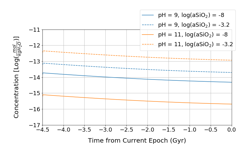
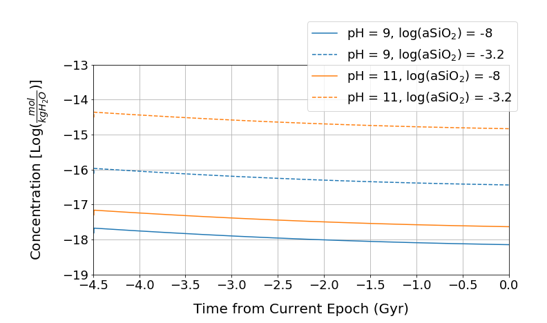
Solving equations 23 and 24 numerically over very short time intervals (1 year), both from and Myr to account for the initial delivery period when both terms equal 0, shows that the O2 and H2O2 concentrations in the ocean are immediately driven to steady-state (the concentrations when the differential terms are set to zero), due to the loss terms dominating the system in both cases. These steady-state concentrations of O2 and H2O2 over time are shown in Figures 7 and 8, and are between and mol/kg H2O and between and mol/kg H2O, respectively. Equivalent figures for Scenario 3, where the ice shell is the only source of oxidants, are provided in Appendix B. In all cases, the resulting steady-state concentration of H2O2 is lower than the concentration of O2 (i.e., H2O2 reacts faster) due to larger loss terms in equations 23 and 24.
As would be expected for an ocean where reductants are far more abundant than oxidants, the concentrations of O2 and H2O2 are very low. However their abiotic consumption produces ferric oxyhydroxides and SO, which could also be biologically useful oxidants. In the case where all oxidants are in the form of O2, we partition the O2 flux into consumption by Fe2+ vs. HS- according to the rates of the respective processes (Equations 11-12 and 15-16), using the calculated steady-state concentration of O2 through time:
| (25) |
| (26) |
where we have again chosen FeOOH to be representative of ferric oxyhydroxide minerals. In the case where all oxidants are in the form of H2O2, we use (derived from equations 13-14 and 17-18):
| (27) |
| (28) |
The results for oxidation by O2 and oxidation by H2O2 are plotted in Figures 9a-b and Figures 9c-d, respectively, with equivalent figures for Scenario 3 provided in Appendix B. We have assumed that FeOOH and SO accumulate in the ocean or at the seafloor as secondary oxidants, where they could be available for use by life, and are not abiotically reduced back to ferrous iron and sulfides. This may be a valid assumption for SO, as available experimental data indicate that sulfate reduction is kinetically inhibited at more alkaline () pH values (Truche et al. 2009 Tan et al. 2019). For ferric iron, the potential for abiotic reduction to occur under Enceladus ocean conditions could be greater. The ability for life to use ferric iron metabolically would depend on the relative rates of biotic versus abiotic iron reduction, as it does in systems on Earth (e.g., Mortimer et al. 2011). Laboratory studies of microorganisms in sediments indicate that iron reduction may not be an important metabolic process for organisms living in alkaline environments [Marquart et al. 2019], meaning abiotic iron reduction may be faster, although competition could still occur to some degree. This underscores the need for future experiments to constrain the abiotic rates of ferric iron reduction in the presence of potential electron donors (H FeS, organic matter) under Enceladus ocean conditions [Glein et al. 2018].
Although the reductant loss terms for H2O2 in equation 24 are larger than those for O2 in equation 23, it is evident from Figure 9 that more of the oxidized products form from O2 than from H2O2 due to reaction stoichiometry (one mole of O2 produces twice as much FeOOH or SO as one mole of H2O2, Equations 11-14). However, in both cases the maximum abundance of FeOOH (10 mmol/kg H2O) corresponds to a situation in which almost all of the O2 or H2O2 available is converted to FeOOH. The only set of considered conditions in which ferrous iron oxidation is not strongly favored, and the amount of SO produced is comparable to the amount of FeOOH produced, is oxidation by O2 at pH = 9 and log(aSiO2) = -3.2.
:

4.3 Case III: Oxidation of Minerals
In our third case, we assume that reductants are present as minerals in the rocky core, and that all ocean water can circulate through the core such that any O2 and H2O2 present is consumed. To determine how the oxidizing power of O2 and H2O2 are distributed between sulfur-bearing minerals and iron-bearing minerals, we first estimate the relative abundances of these minerals in the core, given the simplified mineralogical model of Enceladus’ core from Waite et al. 2017 (supplemental material) and reproduced here in Table 3. We consider both a core composed of reduced hydrous rock (RHR) and a core composed of oxidized hydrous rock (OHR), the two models for which the mass of rock in the interior is provided. We take greenalite (Gre) and magnetite (Mag) to be the iron-bearing mineral that will react with oxidants in a RHR or OHR core, respectively, by:
| Rock type: | Reduced | Oxidized | |
|---|---|---|---|
| hydrous rock | hydrous rock | ||
| Abbreviation: | RHR | OHR | |
| Mineral | Formula | Wt.% Vol.% | Wt.% Vol.% |
| Chrysotile | Mg3Si2O5(OH)4 | 48.86 57.17 | 27.53 32.30 |
| Greenalite | Fe3Si2O5(OH)4 | 29.75 27.59 | - - |
| Magnetite | Fe3O4 | - - | 19.11 11.04 |
| Pyrrhotite | Fe0.875S | 19.27 12.49 | 19.87 12.92 |
| Talc/Saponite | Mg3Si4O10(OH)2 | 2.12 2.76 | 33.49 43.74 |
| (29) |
| (30) |
| (31) |
| (32) |
and pyrrhotite (Po, Fe0.875S) to be the sulfur-bearing mineral that will react with oxidants in both RHR and OHR via:
| (33) |
| (34) |
:

For both the RHR and OHR interiors, we find the molar ratio of the iron-bearing mineral (greenalite or magnetite) to pyrrhotite to be 1:3. Along with relative abundances, we also consider how quickly iron-bearing minerals oxidize compared with sulfur-bearing minerals. We take the weathering rates for FeO and FeS type minerals by O2 on Earth from Walker 1977, and compare the mass of O2 consumed per mass sulfide with the mass of O2 consumed per mass FeO, for a given weight percent ratio of sulfide to FeO, in the rock (Figure 10). Because these weathering rates were derived from a lower pH system than the Enceladus ocean, our extrapolation is missing a pH dependence that could shift the relative rates of iron and sulfur mineral oxidation. However, without weathering data from higher pH systems, we will not consider pH dependence in the current work as it is simply a first attempt to examine how this system might behave, and we emphasize the need for future studies to constrain these rates in alkaline pH environments on Earth.
We find that, for these rocks, sulfide consumes O2 18 times faster per unit mass. We extrapolate this relationship to the weight percent ratio of sulfide to FeO in RHR and OHR rocks on Enceladus, and find that oxidation of sulfide occurs 2.7 times faster than oxidation of FeO in RHR, and 8.1 times faster in OHR, per unit mole. Assuming the relative oxidation rates for H2O2 are comparable, we compute the fraction of O2 and H2O2 consumed by each rock type via:
| (35) |
| (36) |
| (37) |
| (38) |
where N is the number of moles of a given mineral, and the subscripts or in and represent either RHR or OHR, respectively. Given the stoichiometry of reactions 29-34, we calculate the amounts of FeOOH and SO produced through the oxidation of each of these minerals by O2 and H2O2. The results are shown in Figures 11 and 12, with equivalent figures if 40K decay does not act a source of oxidants (Scenario 3, see Table 1) provided in Appendix B.
Unlike Case II, in which all reductants were in aqueous form (Section 4.2), we find that the relative production of SO compared to FeOOH is much closer in all cases, for both oxidation by O2 and H2O2, due to the preference for oxidation of FeS rather than FeO. For oxidation by O2, we calculate an upper limit on [FeOOH] of 2.0-2.2 mmol/kg H2O, and an upper limit on [SO] of 1.0-1.1 mmol/kg H2O. For oxidation by H2O2, we calculate an upper limit on [FeOOH] of 1.0-1.1 mmol/kg H2O, and an upper limit on [SO] of 0.52-0.56 mmol/kg H2O.
:


5 Compatibility with the Available Data
To determine which of the three cases outlined in this paper (see Table 1) may be most appropriate, we can examine how the oxidant concentrations predicted in each case compare with available data from Cassini. In Case I, where reactive reductants in the ocean are either produced slowly or are non-existent, the resulting oxidant concentrations are 2.5 mmol O2/kg H2O or 3.1 mmol H2O2/kg H2O when oxidants are formed in the ice shell and as a result of 40K decay (Scenarios 1 and 2, Table 1), and 1.0 mmol O2/kg H2O or 1.6 mmol H2O2/kg H2O when the ice shell is the only oxidant source (Scenario 3, Table 1). Given that the inferred concentration of CO2 in the ocean from Waite et al. 2017 is between and mmol/kg H2O, this implies that O2 or H2O2 should be 10 to 30,000 times more abundant than CO2 in the ocean. Because CO2 was detected without ambiguity by INMS (Waite et al. 2017), O2 concentrations this high would also have been detected. Measuring H2O2 would have been more complicated because it is highly reactive, making it difficult to detect in situ. Although Newman et al. 2007 reported an H2O2 abundance of with respect to H2O at the tiger stripe region, inferred from Cassini’s Visible and Infrared Mapping Spectrometer (VIMS) observations, this is likely all radiolytically produced at the surface, rather than delivered from the ocean. Some fraction of any delivered H2O2 would, however, dissociate into O2 either during plume transport or in the INMS antechamber. Even if this conversion ratio were small (i.e. at pH 9, and as low as at pH 11), it would yield O2 abundances comparable to CO2 in the plume. INMS did detect a slight increase in mass 32 signal during the E21 flyby with an upper limit of , although the signal to noise of this detection was low and could have been due to catalytic conversion of H2O to H2 and O2 on the walls of the antechamber (Waite et al. 2017, supplemental material).
If we scale the reported upper limit on the O2 mixing ratio in the plume gas to CO2, as we did to determine the upper limit on the concentration of H2S in the ocean in Section 4.2.1, this implies an upper limit on the ocean concentration of O2 between and mol/kg H2O. Thus, while O2 or H2O2 may be present at concentrations higher than those predicted in Case II, observational constraints indicate that their concentrations must still be several orders of magnitude below the concentrations predicted for all scenarios in Case I, if they are present at all. Even if Enceladus is much younger ( Myr old), the O2 or H2O2 concentrations in Case I would only drop by two orders of magnitude (Figure A.16), and would still be comparable to or greater than the concentration of CO2. At these concentrations O2 should still be detectable. However, at pH = 9, where the H2O2 and CO2 concentrations would be comparable (Figure A.16), the O2 trace left by decomposition of H2O2 may not be detectable depending on the fraction of H2O2 decomposed. A young Enceladus with a pH ocean is therefore the only scenario in which Case I cannot be ruled out by constraints from INMS. Even so, aerobic life could still take advantage of the relatively high oxidant fluxes coming from surface ice in Case II and/or Case III if organisms were to reside at the ice-water interface.
Although Case I may be possible under some conditions, there are several lines of evidence that support a hydrothermally active Enceladus (Hsu et al. 2015, Waite et al. 2017, Choblet et al. 2017, Glein et al. 2018), which would both release reductants into the ocean (Case II) and circulate ocean water containing oxidants through the rocky core (Case III). Some support for Case II comes from an ambiguous INMS detection of H2S [Magee & Waite 2017] discussed in Section 4.2.1, which may indicate the presence of sulfide species in the ocean. Both Case II and Case III would also produce SO which was not detected by CDA (Postberg et al. 2009), but the concentrations of SO for these cases in Section 4 all fall close to or below the tentative CDA detection limit of 1mM. The end result of both Case II and Case III are essentially the same (O2 or H2O2 converted to SO or ferric oxyhydroxides), with the primary difference being the final relative abundances of sulfates versus ferric oxyhydroxides and the energy they could provide (see Section 6).
With current observational data it is impossible to determine whether one process may dominate over the other (i.e., whether aqueous reductants consume oxidants before they can be circulated through the rocky core, or vice versa), or whether both are occurring to a comparable extent. A rigorous treatment of hydrothermal geochemistry in the rocky core, incorporating the results of Choblet et al. 2017, is therefore a necessary next step in determining how these two processes may compete with one another and change the final abundances of oxidants in the ocean. Indeed, if circulation occurs deep enough in the core, radiolysis of water caused by the decay of radionuclides in the core (Lin et al. 2005a, Lin et al. 2005b, Bouquet et al. 2017) could act as another source of oxidants to the ocean which could also be incorporated into such a model. Future measurements of sulfur species could also reveal the extent to which oxidation of aqueous reductants versus seafloor/core minerals is occurring. A robust H2S detection, or a detection of ferrous iron, could be used to constrain the concentrations of reduced iron and sulfide species in the ocean and thus the capacity for Case II oxidation to occur. Detection and determination of the ratios of sulfur isotopes in sulfate could also be used not only to confirm the presence of sulfate in the ocean, but also to potentially distinguish between sulfate made from aqueous oxidation of sulfides vs. sulfate that may have formed from sulfur dioxide or elemental sulfur that could have been present in the material from which Enceladus formed.
6 Energy Availability for Metabolic Redox Reactions
To determine whether the abundances of oxidants constrained in Section 4 could be sufficient to provide metabolic energy for life, we calculate chemical affinities for a set of redox reactions, per mole of limiting reactant. These reactions, listed in Tables 4-5 and adapted from Zolotov & Shock 2004 and Amend et al. 2011, encompass many of the major metabolisms used by diverse bacteria and archaea in Earth’s oceans and other inhabited environments. We have included both aerobic and anaerobic organic matter oxidation to represent the possibility for life to oxidize the massive organic compounds (HMOC’s) detected in the plume (Postberg et al. 2018b). As an analog for these compounds, we use kerogen compounds with 404, 415, and 515 carbon atoms described in Helgeson et al. 2009, which well-represent HMOC properties constrained by Postberg et al. 2018b. Because oxidation of these three kerogens have similar equilibrium constants, the resulting chemical affinities and energy fluxes available from these reactions are similar and we have thus reported the average values produced by all three of these compounds in Tables 4 and 5, with an example reaction for oxidation of kerogen with 415 carbon atoms written out explicitly.
With the exception of sulfide and iron oxidation (reactions 2 and 3 in Tables 4 and 5), we have assumed that all of the metabolic reactions listed in Tables 4 and 5 are kinetically inhibited from proceeding abiotically at low temperatures, for the reasons discussed in Section 4. In biology, however, these could proceed, as biocatalysts (i.e. enzymes) can lower the the activation energy barrier.
Chemical affinity serves as a measure of disequilibrium for a given reaction; the greater the magnitude of the chemical affinity, the further out of equilibrium the reaction is (Shock & Canovas 2010, Waite et al. 2017). Chemotrophic life takes advantage of this disequilibrium, extracting energy from the environment to drive the system toward equilibrium (McCollom & Shock 1997, Hoehler et al. 2007). The affinity, , can be calculated via:
| (39) |
where is the gas constant and is the temperature of the ocean assumed to be 273 K. The log - log term in the equation measures the extent to which the activities of the reaction species are out of equilibrium. We calculate equilibrium constants, , from the CHNOSZ package [Dick 2019] at T = 0∘C and P = 73 bar, the approximate pressure at the seafloor [Glein et al. 2018]. We calculate the reaction quotient for each reaction from the thermodynamic activities—or effective concentrations—of oxidants O2, H2O2 and SO and reductants HS- and Fe2+ constrained in Section 4, along with those of H2, CO2 and CH4 derived from INMS detections in Waite et al. 2017. Since FeOOH and Fe0.875S are both minerals and kerogen is a solid, their thermodynamic activity is 1 if the minerals are present as pure phases. In Case III we assume the same activities for HS- and Fe2+ predicted in Case II, as it is likely that the two processes considered in these cases are occurring simultaneously if there is hydrothermal activity on Enceladus. If the concentrations of these reductants were lower, that would only push the reactions they are used in further out of equilibrium, such that the affinities and energy fluxes available would be even higher than the numbers we are reporting. For Case I, we do not consider reactions involving iron or sulfur species, as we have assumed that these reductants are not present.
The chemical affinities for our selected reactions, calculated for each case and scenario outlined in Table 1 and for a young (100 Myr) and old (4.5 Gyr) Enceladus, are shown in Table 4. We use methanogenesis, for which the affinity is less uncertain because it is constrained entirely by observations, as a basis for comparison with all of the other investigated reactions. To determine whether these reactions could be used as metabolisms, we compare their affinities to , the minimum amount of energy required to convert ADP to ATP and therefore be used by life on Earth, which has been measured to be as low as 20 kJ/mol for laboratory cultures and 10 kJ/mol for cells in nature ([Hoehler et al. 2001], [Hoehler 2004]). Methanogenesis clearly meets these requirements for both pH 9 and 11. The affinities for the chosen aerobic reactions are also well above this requirement, even for the Case II values for which the concentrations of O2 and H2O2 are very low (Section 4.2). Although we have assumed aerobic metabolism is not possible in Case III (Section 4.3), life could likely still use some of the O2 and/or H2O2 flux produced in the ocean even if these oxidants were also reacting with minerals. Aerobic reactions could therefore likely support life on Enceladus even if hydrothermal activity were consuming a large portion of the oxidant flux at the same time.
| Metabolic Process | Affinity (kJ mol-1) | ||||||||
| Methanogenesis: | |||||||||
| 4H2 + CO CH4 + 2H2O | 90 30 | ||||||||
| Primary Model | Young Enceladus | No 40K Oxidant Source | |||||||
| Aerobic Reactions | Case I | Case II | Case III | Case I | Case II | Case III | Case I | Case II | Case III |
| 1. Methane Oxidation: | |||||||||
| CH4 + O CO2 + H2O | 420 | 360 10 | NA | 410 | 360 10 | NA | 410 | 360 10 | NA |
| CH4 + H2OCO2 + H2O | 300 | 250 40 | NA | 290 | 250 40 | NA | 300 | 250 40 | NA |
| 2. Oxidation of Sulfides | |||||||||
| HS- + O SO + H+ | NA | 350 10 | NA | NA | 350 10 | NA | NA | 350 10 | NA |
| HS- + H2O SO + H+ +H2O | NA | 220 10 | NA | NA | 220 10 | NA | NA | 220 10 | NA |
| 3. Oxidation of Iron Sulfide | |||||||||
| Fe0.875S + O2 + H2O Fe2+ + SO + H+ | NA | 350 10 | NA | NA | 350 10 | NA | NA | 350 10 | NA |
| Fe0.875S + H2O2 Fe2+ + SO + H+ + H2O | NA | 220 10 | NA | NA | 220 10 | NA | NA | 220 10 | NA |
| 4. Hydrogen Oxidation: | |||||||||
| 2H2 + O 2H2O | 460 10 | 400 10 | NA | 450 10 | 400 10 | NA | 460 10 | 400 10 | NA |
| H2 + H2O 2H2O | 320 10 | 250 10 | NA | 310 10 | 250 10 | NA | 320 10 | 240 10 | NA |
| 5. Aerobic Organic Matter Oxidation: | |||||||||
| C415H698O22 + O2 CO2 + H2O | 440 10 | 370 10 | NA | 430 10 | 370 10 | NA | 440 10 | 370 10 | NA |
| C415H698O22 + H2O2 CO2 + H2O | 310 10 | 240 20 | NA | 300 10 | 240 20 | NA | 310 10 | 240 20 | NA |
| Anaerobic Reactions | Case I | Case II | Case III | Case I | Case II | Case III | Case I | Case II | Case III |
| 1. Sulfate Reduction: | |||||||||
| 4H2 + SO + H 4H2O + HS- | NA | 100 40 | 110 30 | NA | 90 40 | 90 30 | NA | 100 40 | 100 30 |
| 2. Anaerobic Oxidation of Methane: | |||||||||
| CH4 + SO + H CO2 + HS- + 2H2O | NA | 10 10 | 20 | NA | 0 10 | 10 | NA | 10 10 | 20 |
| 3. Reduction of Ferric Iron: | |||||||||
| H2 + FeOOH + 2H 2H2O + Fe2+ | NA | 20 10 | 10 10 | NA | 20 10 | 10 10 | NA | 20 10 | 10 10 |
| 4. Anaerobic Organic Matter Oxidation: | |||||||||
| C415H698O22 + SO + H+ CO2 + HS- + H2O | NA | 70 20 | 80 10 | NA | 60 20 | 70 10 | NA | 70 20 | 70 10 |
| C415H698O22 + FeOOH + 2H+ CO2 + Fe2+ + H2O | NA | 10 10 | 10 10 | NA | 10 10 | 10 10 | NA | 10 10 | 10 10 |
| Metabolic Process | Energy Flux (kJ s-1) | ||||||||
| Methanogenesis: | |||||||||
| 4H2 + CO CH4 + 2H2O | 10,300 7,700 | ||||||||
| Primary Model | Young Enceladus | No 40K Oxidant Source | |||||||
| Aerobic Reactions | Case I | Case II | Case III | Case I | Case II | Case III | Case I | Case II | Case III |
| 1. Methane Oxidation: | |||||||||
| CH4 + O CO2 + H2O | 110 | 90 | NA | 100 | 90 | NA | 80 | 70 | NA |
| CH4 + H2OCO2 + H2O | 110 | 90 10 | NA | 110 | 90 10 | NA | 90 | 70 10 | NA |
| 2. Oxidation of Sulfides | |||||||||
| HS- + O SO + H+ | NA | 90 | NA | NA | 90 | NA | NA | 60 | NA |
| HS- + H2O SO + H+ +H2O | NA | 80 | NA | NA | 80 | NA | NA | 70 | NA |
| 3. Oxidation of Iron Sulfide | |||||||||
| Fe0.875S + O2 + H2O Fe2+ + SO + H+ | NA | 90 | NA | NA | 90 | NA | NA | 60 | NA |
| Fe0.875S + H2O2 Fe2+ + SO + H+ + H2O | NA | 80 10 | NA | NA | 80 | NA | NA | 70 | NA |
| 4. Hydrogen Oxidation: | |||||||||
| 2H2 + O 2H2O | 120 | 100 | NA | 110 | 100 | NA | 80 | 70 | NA |
| H2 + H2O 2H2O | 120 | 90 | NA | 110 | 90 | NA | 100 | 70 | NA |
| 5. Aerobic Organic Matter Oxidation: | |||||||||
| C415H698O22 + O2 CO2 + H2O | 110 | 90 | NA | 110 | 90 | NA | 80 | 70 | NA |
| C415H698O22 + H2O2 CO2 + H2O | 120 | 90 10 | NA | 110 | 90 10 | NA | 90 | 70 | NA |
| Anaerobic Reactions | Case I | Case II | Case III | Case I | Case II | Case III | Case I | Case II | Case III |
| 1. Sulfate Reduction: | |||||||||
| 4H2 + SO + H 4H2O + HS- | NA | 2 15 | 9 6 | NA | 2 14 | 9 6 | NA | 1 10 | 6 5 |
| 2. Anaerobic Oxidation of Methane: | |||||||||
| CH4 + SO + H CO2 + HS- + 2H2O | NA | 0 2 | 2 1 | NA | 0 1 | 1 | NA | 0 1 | 1 |
| 3. Reduction of Ferric Iron: | |||||||||
| H2 + FeOOH + 2H 2H2O + Fe2+ | NA | 11 5 | 3 3 | NA | 11 5 | 3 3 | NA | 8 5 | 2 2 |
| 4. Anaerobic Organic Matter Oxidation: | |||||||||
| C415H698O22 + SO + H+ CO2 + HS- + H2O | NA | 1 7 | 7 3 | NA | 1 6 | 6 2 | NA | 1 5 | 5 2 |
| C415H698O22 + FeOOH + 2H+ CO2 + Fe2+ + H2O | NA | 6 7 | 2 2 | NA | 6 7 | 2 2 | NA | 5 5 | 2 1 |
Because SO and ferric oxyhydroxides are much weaker oxidants than O2, even when they are present in large abundances (as in Case II and Case III) the capacity for anaerobic reactions to meet is largely affected by ocean chemistry, the extent to which water-rock reactions could be occurring on Enceladus, and the time period over which oxidant production could be occurring. Case III represents the most favorable set of conditions for anaerobic reactions to meet . Thus, if ocean water can percolate through the seafloor, particularly at warmer temperatures where aqueous O2 and H2O2 can readily oxidize reduced iron and sulfur-bearing minerals there, then anaerobic reactions could more feasibly serve as an energy source for life in the ocean. In Case II, where seafloor water-rock reactions serve primarily to produce aqueous reductants in the ocean faster than the production of oxidants, but where minerals are not oxidized directly, the capacity for anaerobic reactions to meet the depends strongly on ocean chemistry, and particularly on pH. In a scenario like Case II in which all O2 or H2O2 abiotically oxidizes iron and sulfur in the ocean before it can be used by life, the pH of the ocean would limit which anaerobic metabolisms could support life.
Besides the , another critical factor that determines whether a given redox coupling could actually support life is the flux of that energy source through time. The magnitude of this energy flux determines how much biomass could be created and supported within Enceladus. We convert our affinity values to energy fluxes by multiplying by the production rate of the limiting reactant, which is the oxidant for all reactions besides methanogenesis. The results are reported in Table 5. For methanogenesis, we assume the flux of H2 in the plume, mol yr-1 [Waite et al. 2017], is equal to the production rate of H2 in the ocean. The lower and upper limits on this production rate are reflected in the range of values reported in Table 5. This assumption is valid if the concentration of H2 in the ocean is in steady-state and fractionation in the plume is accounted for. The range of H2 production rates estimated this way is consistent with some values reported from models of serpentinization of Enceladus’ rocky core, including Vance et al. 2016 and the upper limit in Steel et al. 2017. Other reported values range between two orders of magnitude lower (the lower limit reported in Steel et al. 2017) and four to five orders of magnitude lower [Taubner et al. 2018], which would lower the energy flux from methanogenesis proportionally.
We can explore the size of the biosphere that may be supported on Enceladus by comparing our energy flux values to maintenance energy requirements for microbial cells on Earth, or the energy flux required to sustain some amount of biomass (Hoehler 2004 and Hoehler & Jørgensen 2013). Although exact values for maintenance energies are not well constrained, particularly for organisms in nature, we can obtain a general understanding of where the values in Table 5 fall by comparing them to values determined from chemostat cultures ( kJ cell-1 day-1 for anaerobes and kJ cell-1 day-1 for aerobes, Tijhuis et al. 1993 and Hoehler & Jørgensen 2013). These values could, however, be several orders of magnitude lower for organisms living in natural, and particularly in energy-starved, environments (Morita 1997, Morita 1999). We use these values, and the ranges of energy fluxes provided by each reaction in Table 5, to estimate the number of cells that could be supported by these metabolisms in each case (Table 6). For closer comparison to Earth systems, we also calculate theoretical cell densities over a range of possible volumes, with three nominal reference points in which life on Enceladus could be contained: the area of the seafloor directly under the south polar terrain (SPT) where we predict the O2 and H2O2 flux will be highest, the entire seafloor, and the entire ocean volume (Figure 13). For the former two we have considered a range of depths from 1 cm to 20 m, which could encompass microbes in a thin mat at the seafloor or spread down to the Røy et al. 2012 Earth reference point shown on Figure 13. It is possible that microbes could inhabit depths greater than these depending on the temperature in Enceladus’ rocky core, but the resulting cell densities would be even smaller than those reference points reported for Earth from Whitman et al. 1998, Christner et al. 2006 and Røy et al. 2012.
It is evident from both Table 6 and Figure 13 that, while methanogenesis clearly dominates as an energy source at least for the high hydrogen production rates that we have used, all of the potential metabolic reactions considered here could still contribute to supporting a biosphere on Enceladus. The cell densities we have calculated for reactions other than methanogenesis are low compared to values measured on Earth (see Figure 13), but could become comparable to these values if smaller volumes were considered. Although ocean chemistry in Case II can have a significant impact on the capacity for anaerobic metabolisms to support life, some anaerobic metabolisms and all aerobic metabolisms are still able to sustain biomass in each set of conditions we have considered. This is significant not only because it supports the potential for diverse metabolisms on Enceladus, but also because of its implications for how life could have emerged there if the availability of redox species was variable throughout Enceladus’ history. For instance, if there was less tidal heating of Enceladus’ rocky core earlier in its history and H2 availability was more restricted, other redox reactions besides methanogenesis could still provide energy for the development of life.
| Total Cells | |||
| Methanogenesis: | 7.0e20 - 4.8e21 | ||
| Primary Model | Young Enceladus | No 40K Oxidant Source | |
| Case I: Buildup of O2 and H2O2 | |||
| Aerobes: | 1.3e19 - 1.9e19 | 1.2e19 - 1.8e19 | 1.0e19 - 1.5e19 |
| Case II: Oxidation of Aqueous Reductants | |||
| Aerobes: | 8.2e18 - 1.6e19 | 8.2e18 - 1.6e19 | 6.6e18 - 1.3e19 |
| Anaerobes: | 0 - 4.4e18 | 0 - 4.3e18 | 0 - 3.5e18 |
| Case III: Oxidation of Minerals | |||
| Anaerobes: | 5.5e16 - 4.2e18 | 5.5e16 - 3.8e18 | 4.4e16 - 3.0e18 |
If the age of Enceladus is closer to 100 Myr, Tables 4-6 show that the capacity for the ocean to sustain life does not appreciably change from an energetic standpoint. Although the final concentrations of oxidants in the ocean decrease by one to two orders of magnitude (with the exception of the steady-state concentrations of O2 and H2O2 in Case II, which are the same - see Appendix A), the resulting affinities drop by only 10-20 kJ/mol, if at all. This only affects the potential for a few anaerobic reactions to meet the , while the affinities for all aerobic and most anaerobic metabolisms still exceed this threshold. Because the production rates of oxidants at present day are the same regardless of the age of Enceladus, the energy fluxes are affected only by affinity and thus are also either unchanged or decreased by only 10 kJ s-1 or less. The cell counts resulting from these decreased fluxes would only drop by 10 or less (Table 6). The production rates, and the resulting energy fluxes and supported cell densities, could be further decreased if the surface at the tiger stripe region was less active, or not active at all earlier in Enceladus’ history. However, even if the surface contribution to the O2 and H2O2 production rate was effectively cut off, oxidant production by decay would persist as long as there was an ocean present, unless aqueous reductants caused significant interference with oxidant production (Scenario 3). Furthermore, because the rate of radiolytic oxidant production by 40K decay decreases through time (Appendix C, Figure C.27), the energy flux available from our selected reactions could have been higher earlier in Enceladus’ history, even if the contribution from the surface were smaller. In the case of a 4.5 Gyr old Enceladus, the O2 or H2O2 production rates are dominated by decay for the first or Gyr, respectively, which would result in higher energy fluxes even if there were no oxidants delivered from the surface during this time. Thus, even for a younger Enceladus and variable surface overturn rates, our chosen redox couplings might still be exploited as energy sources by microbial life in the ocean.
The Enceladus ocean’s ability to sustain life similarly does not change appreciably if there is no oxidant production from 40K decay, a possibility discussed in Section 3. While the total oxidant availability in all three cases is lowered by up to an order of magnitude (Appendix B), the chemical affinities do not drop by more than 10 kJ/mole at most (see Table 4). The energy fluxes are slightly more sensitive to this potential decrease in oxidant availability, as they also depend on the oxidant production rate and would be up to 30 kJ s-1 lower for aerobic reactions, and up to 5 kJ s-1 lower for anaerobic reactions (see Table 5). The resulting total number of cells that could be made would thus decrease by 20-30 . However, as with a younger Enceladus age, this hardly affects the size of the biosphere (i.e. the cell densities) that could be sustained.

7 Conclusions
We have shown that the production of radiolytic oxidants on Enceladus could lead to redox disequilibria in the ocean, which could provide energy to support putative life. Radiolysis of surface ice, coupled with transport of ice to the ocean in the geologically active tiger stripe region, can deliver up to moles of O2 and moles of H2O2. Electrons and gamma rays released as a result of the decay of 40K atoms in the ocean can produce another moles of O2 and moles of H2O2 directly in the ocean. These radiolytic oxidants may build up in the ocean if the availability of reactive reductants is limited, or they could be converted to SO and ferric oxyhydroxides if water-rock interactions control the redox chemistry of the ocean. In the former case, the resulting ocean concentrations of oxidants (2.5 mmol O2/kg H2O or 3.1 mmol H2O2/kg H2O) are much higher than the concentration range for CO2 estimated in Waite et al. 2017 for pH 9 to 11, and thus these oxidants would likely have been detected by the INMS instrument on Cassini.
The absence of a non-ambiguous detection of O2, along with existing evidence that Enceladus is hydrothermally active, instead support a scenario in which radiolytic O2 and H2O2 are converted to SO and ferric oxyhydroxides, by oxidation of aqueous reductants in the ocean (Case II) and/or oxidation of reduced minerals at the seafloor (Case III). The end results of these two cases differ only in the relative abundances of SO versus ferric oxydroxides produced, and predict similar final SO concentrations (mmol/kg H2O or less, depending on ocean chemistry and seafloor mineralogy). Thus, the nominal 1 mmol/kg H2O upper limit on [SO] from the CDA instrument cannot be used to determine which process might dominate over the other. Ongoing laboratory experiments, coupled with continued analysis of the large dataset returned by Cassini CDA, are expected to further constrain the tentative upper limit for SO in Enceladus’ ocean given here. An ambiguous detection of H2S by INMS suggests that reactive reductants could be present, but whether these reductants can consume radiolytic oxidants before they are circulated through the rocky core depends on the relative time scales of each process. Further modeling of the hydrothermal flow of fluid through Enceladus’ seafloor and deeper interior, along with future measurements of S isotopes, would help determine the extent to which each of these processes contributes to the reduction of radiolytic oxidants, and therefore how O2 and H2O2 are partitioned into iron versus sulfide oxidation.
We have shown that, in addition to methanogenesis, aerobic and/or anaerobic reactions in each of our three cases can meet the minimum free energy requirement for terrestrial life, , and provide maintenance energy to support cellular life within Enceladus. Although we have favored Cases II and III, aerobic metabolisms using oxidant fluxes close to those predicted in Case I could still support more than cells at the ice-water interface where radiolytic oxidants from the surface are delivered. Aerobic metabolisms could also sustain another cells in the ocean/seafloor if there are still low ( mol/kg H2O in Case II) ocean concentrations of O2 and/or H2O2. Anaerobic metabolisms could not sustain as much biomass as aerobic metabolisms due to their lower free energy yields, but at least some of these reactions are still viable and could support cells in Case II and Case III. Radiolytic oxidant production and redox chemistry in Enceladus’ ocean and seafloor are therefore capable of supporting metabolic processes beyond methanogenesis, generating the possibility for a metabolically diverse microbial community in the ocean of Enceladus.
Appendix A Oxidant Production on a Young Enceladus
Appendix B Oxidant Production Without a Source
Appendix C Production Rates of Radiolytic Oxidants
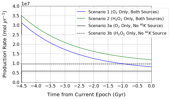
Acknowledgements
This work was supported by the Cassini INMS subcontract from NASA JPL (NASA contract NAS703001TONMO711123, JPL subcontract 1405853) and the Cassini Project; C.R.G. was also supported by the NASA Astrobiology Institute. Support for T.M.H. was provided by NASA’s Planetary Science Division Research Program. The work of F.P. was supported by the European Research Council (ERC Consolidator Grant 724908-Habitat OASIS). The NSF Center for Dark Energy Biosphere Investigations (C-DEBI OCE-0939564) and NASA ICEE2 grant 80NSSC19K0611 supported the participation of J.A.H.
References
- Ab Rahim et al. [2013] Ab Rahim, M. H., Forde, M. M., Jenkins, R. L., Hammond, C., He, Q., Dimitratos, N., Lopez-Sanchez, J. A., Carley, A. F., Taylor, S. H., Willock, D. J. et al. (2013). Oxidation of methane to methanol with hydrogen peroxide using supported gold–palladium alloy nanoparticles. Angewandte Chemie International Edition, 52, 1280–1284.
- Altair et al. [2018] Altair, T., de Avellar, M. G., Rodrigues, F., & Galante, D. (2018). Microbial habitability of europa sustained by radioactive sources. Scientific reports, 8, 260.
- Amend et al. [2011] Amend, J. P., McCollom, T. M., Hentscher, M., & Bach, W. (2011). Catabolic and anabolic energy for chemolithoautotrophs in deep-sea hydrothermal systems hosted in different rock types. Geochimica et Cosmochimica Acta, 75, 5736–5748.
- Berger et al. [2005] Berger, M., Coursey, M., J.S.and Zucker, & Chang, J. (2005). Estar, pstar, and astar: Computer programs for calculating stopping-power and range tables for electrons, protons, and helium ions (version 1.2.3). [online]. Available: http://physics.nist.gov/Star [2018, November 26].
- Bethke [2007] Bethke, C. M. (2007). Geochemical and biogeochemical reaction modeling. Cambridge University Press.
- Bjergbakke et al. [1989a] Bjergbakke, E., Draganić, Z., Sehested, K., & Draganić, I. (1989a). Radiolytic products in waters, part i: Computer simulation of some radiolytic processes in the laboratory. Radiochimica Acta, 48, 73–78.
- Bjergbakke et al. [1989b] Bjergbakke, E., Draganić, Z., Sehested, K., & Draganić, I. (1989b). Radiolytic products in waters, part ii: Computer simulation of some radiolytic processes in nature. Radiochimica Acta, 48, 73–78.
- Bouquet et al. [2019] Bouquet, A., Glein, C. R., & Waite Jr, J. H. (2019). How adsorption affects the gas–ice partitioning of organics erupted from enceladus. The Astrophysical Journal, 873, 28.
- Bouquet et al. [2017] Bouquet, A., Glein, C. R., Wyrick, D., & Waite, J. H. (2017). Alternative energy: Production of h2 by radiolysis of water in the rocky cores of icy bodies. The Astrophysical Journal Letters, 840, L8.
- Čadek et al. [2016] Čadek, O., Tobie, G., Van Hoolst, T., Massé, M., Choblet, G., Lefèvre, A., Mitri, G., Baland, R.-M., Běhounková, M., Bourgeois, O. et al. (2016). Enceladus’s internal ocean and ice shell constrained from cassini gravity, shape, and libration data. Geophysical Research Letters, .
- Chang & Berner [1999] Chang, S., & Berner, R. A. (1999). Coal weathering and the geochemical carbon cycle. Geochimica et Cosmochimica Acta, 63, 3301–3310.
- Choblet et al. [2017] Choblet, G., Tobie, G., Sotin, C., Běhounková, M., Čadek, O., Postberg, F., & Souček, O. (2017). Powering prolonged hydrothermal activity inside enceladus. Nature Astronomy, 1, 841.
- Christner et al. [2006] Christner, B. C., Royston-Bishop, G., Foreman, C. M., Arnold, B. R., Tranter, M., Welch, K. A., Lyons, W. B., Tsapin, A. I., Studinger, M., & Priscu, J. C. (2006). Limnological conditions in subglacial lake vostok, antarctica. Limnology and Oceanography, 51, 2485–2501.
- Chyba & Hand [2001] Chyba, C. F., & Hand, K. P. (2001). Life without photosynthesis. Science, 292, 2026–2027.
- Ćuk et al. [2016] Ćuk, M., Dones, L., & Nesvornỳ, D. (2016). Dynamical evidence for a late formation of saturn’s moons. The Astrophysical Journal, 820, 97.
- Cuzzi et al. [2018] Cuzzi, J., Filacchione, G., & Marouf, E. (2018). The rings of saturn. Problemy Sluchainogo Poiska, (pp. 51–92).
- Davila et al. [2008] Davila, A. F., Fairén, A. G., Gago-Duport, L., Stoker, C., Amils, R., Bonaccorsi, R., Zavaleta, J., Lim, D., Schulze-Makuch, D., & McKay, C. P. (2008). Subsurface formation of oxidants on mars and implications for the preservation of organic biosignatures. Earth and Planetary Science Letters, 272, 456–463.
- Dick [2019] Dick, J. M. (2019). Chnosz: Thermodynamic calculations and diagrams for geochemistry. Frontiers in Earth Science, 7, 180.
- Draganić et al. [1991] Draganić, I., Bjergbakke, E., Draganić, Z., & Sehested, K. (1991). Decomposition of ocean waters by potassium-40 radiation 3800 ma ago as a source of oxygen and oxidizing species. precambrian Research, 52, 337–345.
- Foustoukos et al. [2011] Foustoukos, D. I., Houghton, J. L., Seyfried Jr, W. E., Sievert, S. M., & Cody, G. D. (2011). Kinetics of h2–o2–h2o redox equilibria and formation of metastable h2o2 under low temperature hydrothermal conditions. Geochimica et Cosmochimica Acta, 75, 1594–1607.
- Gaidos et al. [1999] Gaidos, E. J., Nealson, K. H., & Kirschvink, J. L. (1999). Life in ice-covered oceans. Science, 284, 1631–1633.
- Glein et al. [2018] Glein, C., Postberg, F., & Vance, S. (2018). The geochemistry of enceladus: Composition and controls. Enceladus and the Icy Moons of Saturn, (p. 39).
- Glein et al. [2015] Glein, C. R., Baross, J. A., & Waite, J. H. (2015). The ph of enceladus’ ocean. Geochimica et Cosmochimica Acta, 162, 202–219.
- Glein & Waite [2020] Glein, C. R., & Waite, J. H. (2020). The carbonate geochemistry of enceladus’ ocean. Geophysical Research Letters, 47, e2019GL085885.
- Hand et al. [2007] Hand, K. P., Carlson, R. W., & Chyba, C. F. (2007). Energy, chemical disequilibrium, and geological constraints on europa. Astrobiology, 7, 1006–1022.
- Helgeson et al. [2009] Helgeson, H. C., Richard, L., McKenzie, W. F., Norton, D. L., & Schmitt, A. (2009). A chemical and thermodynamic model of oil generation in hydrocarbon source rocks. Geochimica et Cosmochimica Acta, 73, 594–695.
- Hoehler [2004] Hoehler, T. (2004). Biological energy requirements as quantitative boundary conditions for life in the subsurface. Geobiology, 2, 205–215.
- Hoehler et al. [2001] Hoehler, T. M., Alperin, M. J., Albert, D. B., & Martens, C. S. (2001). Apparent minimum free energy requirements for methanogenic archaea and sulfate-reducing bacteria in an anoxic marine sediment. FEMS Microbiology Ecology, 38, 33–41.
- Hoehler et al. [2007] Hoehler, T. M., Amend, J. P., & Shock, E. L. (2007). A “follow the energy” approach for astrobiology. Astrobiology, 7, 819–823.
- Hoehler & Jørgensen [2013] Hoehler, T. M., & Jørgensen, B. B. (2013). Microbial life under extreme energy limitation. Nature Reviews Microbiology, 11, 83.
- Hsu et al. [2015] Hsu, H.-W., Postberg, F., Sekine, Y., Shibuya, T., Kempf, S., Horányi, M., Juhász, A., Altobelli, N., Suzuki, K., Masaki, Y. et al. (2015). Ongoing hydrothermal activities within enceladus. Nature, 519, 207–210.
- Iess et al. [2014] Iess, L., Stevenson, D., Parisi, M., Hemingway, D., Jacobson, R., Lunine, J., Nimmo, F., Armstrong, J., Asmar, S., Ducci, M. et al. (2014). The gravity field and interior structure of enceladus. Science, 344, 78–80.
- Johnson et al. [2013] Johnson, R. E., Carlson, R. W., Cassidy, T. A., & Fama, M. (2013). Sputtering of ices. In The science of solar system ices (pp. 551–581). Springer.
- Khawaja et al. [2019] Khawaja, N., Postberg, F., Hillier, J., Klenner, F., Kempf, S., Nölle, L., Reviol, R., Zou, Z., & Srama, R. (2019). Low-mass nitrogen-, oxygen-bearing, and aromatic compounds in enceladean ice grains. Monthly Notices of the Royal Astronomical Society, 489, 5231–5243.
- LaVerne & Mozumder [1985] LaVerne, J. A., & Mozumder, A. (1985). Range and range straggling of low-energy electrons in the rare gases. The Journal of Physical Chemistry, 89, 4219–4225.
- Le Gall et al. [2017] Le Gall, A., Leyrat, C., Janssen, M. A., Choblet, G., Tobie, G., Bourgeois, O., Lucas, A., Sotin, C., Howett, C., Kirk, R. et al. (2017). Thermally anomalous features in the subsurface of enceladus’s south polar terrain. Nature Astronomy, 1, 0063.
- Li et al. [2016] Li, L., Wing, B., Bui, T., McDermott, J., Slater, G., Wei, S., Lacrampe-Couloume, G., & Lollar, B. S. (2016). Sulfur mass-independent fractionation in subsurface fracture waters indicates a long-standing sulfur cycle in precambrian rocks. Nature communications, 7, 1–9.
- Lin et al. [2005a] Lin, L.-H., Hall, J., Lippmann-Pipke, J., Ward, J. A., Sherwood Lollar, B., DeFlaun, M., Rothmel, R., Moser, D., Gihring, T. M., Mislowack, B. et al. (2005a). Radiolytic h2 in continental crust: nuclear power for deep subsurface microbial communities. Geochemistry, Geophysics, Geosystems, 6.
- Lin et al. [2005b] Lin, L.-H., Slater, G. F., Lollar, B. S., Lacrampe-Couloume, G., & Onstott, T. (2005b). The yield and isotopic composition of radiolytic h 2, a potential energy source for the deep subsurface biosphere. Geochimica et Cosmochimica Acta, 69, 893–903.
- Lodders [2003] Lodders, K. (2003). Solar system abundances and condensation temperatures of the elements. The Astrophysical Journal, 591, 1220.
- Magee & Waite [2017] Magee, B., & Waite, J. (2017). Neutral gas composition of enceladus’ plume–model parameter insights from cassini-inms. In Lunar and Planetary Science Conference. volume 48.
- Marquart et al. [2019] Marquart, K. A., Haller, B. R., Paper, J. M., Flynn, T. M., Boyanov, M. I., Shodunke, G., Gura, C., Jin, Q., & Kirk, M. F. (2019). Influence of ph on the balance between methanogenesis and iron reduction. Geobiology, 17, 185–198.
- McCollom & Shock [1997] McCollom, T. M., & Shock, E. L. (1997). Geochemical constraints on chemolithoautotrophic metabolism by microorganisms in seafloor hydrothermal systems. Geochimica et cosmochimica acta, 61, 4375–4391.
- McDonald et al. [1998] McDonald, G. D., de Vanssay, E., & Buckley, J. R. (1998). Oxidation of organic macromolecules by hydrogen peroxide: implications for stability of biomarkers on mars. Icarus, 132, 170–175.
- McKay et al. [2018] McKay, C., Davila, A., Glein, C., Hand, K., & Stockton, A. (2018). Enceladus astrobiology, habitability, and the origin of life. Enceladus and the Icy Moons of Saturn; Schenk, PM, Clark, RN, Howett, CJA, Verbiscer, AJ, Waite, JH, Eds, (pp. 437–452).
- McKinnon et al. [2018] McKinnon, W., Lunine, J., Mousis, O., Waite, J., & Zolotov, M. (2018). The mysterious origin of enceladus: A compositional perspective. Enceladus and the Icy Moons of Saturn, (p. 17).
- McKinnon [2015] McKinnon, W. B. (2015). Effect of enceladus’s rapid synchronous spin on interpretation of cassini gravity. Geophysical Research Letters, 42, 2137–2143.
- Mikutta et al. [2005] Mikutta, R., Kleber, M., Kaiser, K., & Jahn, R. (2005). Organic matter removal from soils using hydrogen peroxide, sodium hypochlorite, and disodium peroxodisulfate. Soil science society of America journal, 69, 120–135.
- Millero et al. [1987a] Millero, F. J., Hubinger, S., Fernandez, M., & Garnett, S. (1987a). Oxidation of h2s in seawater as a function of temperature, ph, and ionic strength. Environmental science & technology, 21, 439–443.
- Millero et al. [1989] Millero, F. J., LeFerriere, A., Fernandez, M., Hubinger, S., & Hershey, J. P. (1989). Oxidation of hydrogen sulfide with hydrogen peroxide in natural waters. Environmental science & technology, 23, 209–213.
- Millero & Sotolongo [1989] Millero, F. J., & Sotolongo, S. (1989). The oxidation of fe (ii) with h2o2 in seawater. Geochimica et Cosmochimica Acta, 53, 1867–1873.
- Millero et al. [1987b] Millero, F. J., Sotolongo, S., & Izaguirre, M. (1987b). The oxidation kinetics of fe (ii) in seawater. Geochimica et Cosmochimica Acta, 51, 793–801.
- Morita [1999] Morita, R. (1999). Is h 2 the universal energy source for long-term survival? Microbial ecology, 38, 307–320.
- Morita [1997] Morita, R. Y. (1997). Bacteria in oligotrophic environments. Chapman & Hall.
- Mortimer et al. [2011] Mortimer, R. J., Galsworthy, A. M., Bottrell, S. H., Wilmot, L. E., & Newton, R. J. (2011). Experimental evidence for rapid biotic and abiotic reduction of fe (iii) at low temperatures in salt marsh sediments: a possible mechanism for formation of modern sedimentary siderite concretions. Sedimentology, 58, 1514–1529.
- Neveu & Rhoden [2019] Neveu, M., & Rhoden, A. R. (2019). Evolution of saturn’s mid-sized moons. Nature Astronomy, (p. 1).
- Newman et al. [2007] Newman, S., Buratti, B., Jaumann, R., Bauer, J., & Momary, T. (2007). Hydrogen peroxide on enceladus. The Astrophysical Journal Letters, 670, L143.
- Noll et al. [1997] Noll, K., Roush, T., Cruikshank, D., Johnson, R., & Pendleton, Y. (1997). Detection of ozone on saturn’s satellites rhea and dione. Nature, 388, 45–47.
- Paranicas et al. [2012] Paranicas, C., Roussos, E., Krupp, N., Kollmann, P., Hendrix, A., Cassidy, T., Johnson, R., Schenk, P., Jones, G., Carbary, J. et al. (2012). Energetic charged particle weathering of saturn’s inner satellites. Planetary and Space Science, 61, 60–65.
- Park et al. [2003] Park, E. D., Hwang, Y.-S., Lee, C. W., & Lee, J. S. (2003). Copper-and vanadium-catalyzed methane oxidation into oxygenates with in situ generated h2o2 over pd/c. Applied Catalysis A: General, 247, 269–281.
- Pasek [2020] Pasek, M. A. (2020). Plume sample modification at icy moons: Implications for biosignatures. Frontiers in Astronomy and Space Sciences, 7, 14.
- Pierrard & Lazar [2010] Pierrard, V., & Lazar, M. (2010). Kappa distributions: theory and applications in space plasmas. Solar Physics, 267, 153–174.
- Postberg et al. [2018a] Postberg, F., Clark, R. N., Hansen, C. J., Coates, A. J., Ore, C. D., Scipioni, F., Hedman, M. M., & Waite, J. H. (2018a). Plume and surface composition of enceladus. Enceladus and the Icy Moons of Saturn, (p. 129).
- Postberg et al. [2009] Postberg, F., Kempf, S., Schmidt, J., Brilliantov, N., Beinsen, A., Abel, B., Buck, U., & Srama, R. (2009). Sodium salts in e-ring ice grains from an ocean below the surface of enceladus. Nature, 459, 1098–1101.
- Postberg et al. [2018b] Postberg, F., Khawaja, N., Abel, B., Choblet, G., Glein, C. R., Gudipati, M. S., Henderson, B. L., Hsu, H.-W., Kempf, S., Klenner, F. et al. (2018b). Macromolecular organic compounds from the depths of enceladus. Nature, 558, 564.
- Postberg et al. [2011] Postberg, F., Schmidt, J., Hillier, J., Kempf, S., & Srama, R. (2011). A salt-water reservoir as the source of a compositionally stratified plume on enceladus. Nature, 474, 620–622.
- Reynolds et al. [1983] Reynolds, R. T., Squyres, S. W., Colburn, D. S., & McKay, C. P. (1983). On the habitability of europa. Icarus, 56, 246–254.
- Røy et al. [2012] Røy, H., Kallmeyer, J., Adhikari, R. R., Pockalny, R., Jørgensen, B. B., & D’Hondt, S. (2012). Aerobic microbial respiration in 86-million-year-old deep-sea red clay. Science, 336, 922–925.
- Satterfield & Case [1954] Satterfield, C. N., & Case, L. C. (1954). Reaction of aldehyde and hydrogen peroxide in aqueous solution. Industrial & Engineering Chemistry, 46, 998–1001.
- Schippers et al. [2008] Schippers, P., Blanc, M., André, N., Dandouras, I., Lewis, G., Gilbert, L., Persoon, A., Krupp, N., Gurnett, D., Coates, A. et al. (2008). Multi-instrument analysis of electron populations in saturn’s magnetosphere. Journal of Geophysical Research: Space Physics, 113.
- Seki et al. [2000] Seki, Y., Min, J. S., Misono, M., & Mizuno, N. (2000). Reaction mechanism of oxidation of methane with hydrogen peroxide catalyzed by 11-molybdo-1-vanadophosphoric acid catalyst precursor. The Journal of Physical Chemistry B, 104, 5940–5944.
- Sekine et al. [2015] Sekine, Y., Shibuya, T., Postberg, F., Hsu, H.-W., Suzuki, K., Masaki, Y., Kuwatani, T., Mori, M., Hong, P. K., Yoshizaki, M. et al. (2015). High-temperature water–rock interactions and hydrothermal environments in the chondrite-like core of enceladus. Nature communications, 6, 8604.
- Shilov & Shul’pin [2001] Shilov, A. E., & Shul’pin, G. B. (2001). Activation and catalytic reactions of saturated hydrocarbons in the presence of metal complexes volume 21. Springer Science & Business Media.
- Shock & Canovas [2010] Shock, E., & Canovas, P. (2010). The potential for abiotic organic synthesis and biosynthesis at seafloor hydrothermal systems. Geofluids, 10, 161–192.
- Sittler et al. [2004] Sittler, E. C., Johnson, R., Jurac, S., Richardson, J., McGrath, M., Crary, F., Young, D., & Nordholt, J. (2004). Pickup ions at dione and enceladus: Cassini plasma spectrometer simulations. Journal of Geophysical Research: Space Physics, 109.
- Sittler Jr et al. [2006] Sittler Jr, E., Thomsen, M., Johnson, R., Hartle, R., Burger, M., Chornay, D., Shappirio, M., Simpson, D., Smith, H., Coates, A. et al. (2006). Cassini observations of saturn’s inner plasmasphere: Saturn orbit insertion results. Planetary and Space Science, 54, 1197–1210.
- Sorokin et al. [2010] Sorokin, A., Kudrik, E., Alvarez, L., Afanasiev, P., Millet, J., & Bouchu, D. (2010). Oxidation of methane and ethylene in water at ambient conditions. Catalysis Today, 157, 149–154.
- Southworth et al. [2019] Southworth, B. S., Kempf, S., & Spitale, J. (2019). Surface deposition of the enceladus plume and the zenith angle of emissions. Icarus, 319, 33–42.
- Steel et al. [2017] Steel, E. L., Davila, A., & McKay, C. P. (2017). Abiotic and biotic formation of amino acids in the enceladus ocean. Astrobiology, 17, 862–875.
- Tan et al. [2019] Tan, S., Sekine, Y., Shibuya, T., Miyamoto, C., & Takahashi, Y. (2019). Hydrothermal sulfate reduction as a possible sink of sulfate in Europa. In Goldschmidt Abstracts.
- Taubner et al. [2018] Taubner, R.-S., Pappenreiter, P., Zwicker, J., Smrzka, D., Pruckner, C., Kolar, P., Bernacchi, S., Seifert, A. H., Krajete, A., Bach, W. et al. (2018). Biological methane production under putative enceladus-like conditions. Nature communications, 9, 748.
- Teolis et al. [2017a] Teolis, B., Plainaki, C., Cassidy, T., & Raut, U. (2017a). Water ice radiolytic o2, h2, and h2o2 yields for any projectile species, energy, or temperature: A model for icy astrophysical bodies. Journal of Geophysical Research: Planets, 122, 1996–2012.
- Teolis et al. [2009] Teolis, B., Shi, J., & Baragiola, R. (2009). Formation, trapping, and ejection of radiolytic o 2 from ion-irradiated water ice studied by sputter depth profiling. The Journal of chemical physics, 130, 134704.
- Teolis et al. [2005] Teolis, B., Vidal, R., Shi, J., & Baragiola, R. (2005). Mechanisms of o 2 sputtering from water ice by kev ions. Physical Review B, 72, 245422.
- Teolis et al. [2017b] Teolis, B. D., Perry, M. E., Hansen, C. J., Waite, J. H., Porco, C. C., Spencer, J. R., & Howett, C. J. (2017b). Enceladus plume structure and time variability: Comparison of cassini observations. Astrobiology, 17, 926–940.
- Thomas et al. [2016] Thomas, P., Tajeddine, R., Tiscareno, M., Burns, J., Joseph, J., Loredo, T., Helfenstein, P., & Porco, C. (2016). Enceladus’s measured physical libration requires a global subsurface ocean. Icarus, 264, 37–47.
- Tijhuis et al. [1993] Tijhuis, L., Van Loosdrecht, M. C., & Heijnen, J. (1993). A thermodynamically based correlation for maintenance gibbs energy requirements in aerobic and anaerobic chemotrophic growth. Biotechnology and bioengineering, 42, 509–519.
- Truche et al. [2009] Truche, L., Berger, G., Destrigneville, C., Pages, A., Guillaume, D., Giffaut, E., & Jacquot, E. (2009). Experimental reduction of aqueous sulphate by hydrogen under hydrothermal conditions: implication for the nuclear waste storage. Geochimica et Cosmochimica Acta, 73, 4824–4835.
- Vance et al. [2016] Vance, S., Hand, K., & Pappalardo, R. (2016). Geophysical controls of chemical disequilibria in europa. Geophysical Research Letters, .
- Waite et al. [2017] Waite, J. H., Glein, C. R., Perryman, R. S., Teolis, B. D., Magee, B. A., Miller, G., Grimes, J., Perry, M. E., Miller, K. E., Bouquet, A. et al. (2017). Cassini finds molecular hydrogen in the enceladus plume: Evidence for hydrothermal processes. Science, 356, 155–159.
- Waite Jr et al. [2009] Waite Jr, J. H., Lewis, W., Magee, B., Lunine, J., McKinnon, W., Glein, C., Mousis, O., Young, D., Brockwell, T., Westlake, J. et al. (2009). Liquid water on enceladus from observations of ammonia and 40ar in the plume. Nature, 460, 487–490.
- Walker [1977] Walker, J. C. (1977). Evolution of the Atmosphere. MacMillan Publishing Co., Inc.
- Webley & Tester [1991] Webley, P. A., & Tester, J. W. (1991). Fundamental kinetics of methane oxidation in supercritical water. Energy & fuels, 5, 411–419.
- Whitman et al. [1998] Whitman, W. B., Coleman, D. C., & Wiebe, W. J. (1998). Prokaryotes: the unseen majority. Proceedings of the National Academy of Sciences, 95, 6578–6583.
- Wilson et al. [2008] Wilson, R., Tokar, R., Henderson, M., Hill, T., Thomsen, M., & Pontius Jr, D. (2008). Cassini plasma spectrometer thermal ion measurements in saturn’s inner magnetosphere. Journal of Geophysical Research: Space Physics, 113.
- Zolotov [2007] Zolotov, M. Y. (2007). An oceanic composition on early and today’s enceladus. Geophysical research letters, 34.
- Zolotov & Shock [2004] Zolotov, M. Y., & Shock, E. L. (2004). A model for low-temperature biogeochemistry of sulfur, carbon, and iron on europa. Journal of Geophysical Research: Planets, 109.