Probing Inflation with Precision Bispectra
Abstract
Calculating the primordial bispectrum predicted by a model of inflation and comparing it to what we see in the sky is very computationally intensive, necessitating layers of approximations and limiting the models which can be constrained. Exploiting the inherent separability of the tree level in-in formalism using expansions in separable basis functions provides a means by which to obviate some of these difficulties. Here, we develop this approach further into a practical and efficient numerical methodology which can be applied to a much wider and more complicated range of bispectrum phenomenology, making an important step forward towards observational pipelines which can directly confront specific models of inflation. We describe a simple augmented Legendre polynomial basis and its advantages, then test the method on single-field inflation models with non-trivial phenomenology, showing that our calculation of these coefficients is fast and accurate to high orders.
1 Introduction
The primordial bispectrum is one of the main characteristics used to distinguish between models of inflation. While it is well known that the physics of inflation must have been extremely close to linear, and the initial seeds of structure it laid down very close to Gaussian, there is expected to have been some level of coupling between the Fourier modes of the perturbations. In the simplest example of an inflation model this is expected to be unobservable [1], but the possibility remains that inflation was driven by more complex physics that may have left an observable imprint on our universe today. Some models of inflation have interactions that predict non-Gaussian correlations at observable levels. Ways this can happen include self-interactions [2, 3], interactions between multiple fields [4], sharp features [5] and periodic features [6]. However, constraining such imprints is extremely difficult observationally. Even once the data has been obtained, using existing methods it is extremely computationally intensive to translate this into constraints on specific inflation scenarios. Much progress has been made by course-graining the model space into a small number of approximate templates, and leveraging the simplifying characteristic of separability with respect to the three parameters of the bispectrum [7, 8].
The primordial bispectrum is the Fourier equivalent of the three-point correlator of the primordial curvature perturbation. If this field is Gaussian, the bispectrum vanishes, so it is a valuable measure of the interactions in play during inflation. If some inflation model predicts a bispectrum that is sufficiently well approximated by the standard separable templates, the constraints on those standard templates can be translated into constraints on the parameters of the model. The fact that all primordial templates estimated thus far from the CMB are consistent with zero has already provided such constraints in certain scenarios [9, 10]. With this high-precision Planck data, and data from forthcoming experiments such as the Simons Observatory (SO) [11] and CMB-S4 [12], robust pipelines must be developed to circumvent the computational difficulties and extract the maximum amount of information possible. Due to the nature of bispectrum estimation in the CMB and LSS [13, 14, 15, 16] constraining an arbitrary template is difficult. Our aim in this work is to develop the inflationary part of a pipeline to allow to efficiently test a much broader range of models. In this work, we explore shapes arising from tree-level effects in single field models. We do this numerically, allowing quantitative results for a broad range of models, and avoiding extra approximations. Our general aim is to apply the modal philosophy of [17, 18, 19] to calculating primordial bispectra. This modal philosophy is a flexible method that has broadened the range of constrained bispectrum templates, by expanding them in a carefully chosen basis. The Modal estimator is thus capable of constraining non-separable templates, while the KSW estimator cannot. In this work we exploit the intrinsic separability of the tree-level in-in formalism to apply these methods at the level of inflation. Expressing the primordial bispectrum in a separable basis expansion leads to vast increases in efficiency both at the primordial and late-universe parts of the calculation. The main advantage is that expressing the primordial shape function in this way reduces the process of bispectrum estimation in the CMB to a cost which is large, but need only be paid once per basis, not per scenario. A proof of concept of this approach at the primordial level was presented in [20], and the details of the bispectrum estimation part will be detailed in [21]. We go beyond the work of [20] both in developing the choice of basis (the feasibility of the method depending vitally on the chosen basis achieving sufficiently fast convergence in a broad range of interesting models) and in the methods we use to allow us to go to much higher order in our modal expansion, allowing us to apply the method to feature bispectra for the first time.
The paper is organised as follows. In section 2 we present brief reviews of the various parts of the pipeline that connects inflation scenarios to observations through the bispectrum. We review the usual paradigm of bispectrum estimation in the CMB, and the motivation for separable bispectra. We review the in-in formalism, for calculating the tree level bispectrum for a given model of inflation. We review models of inflation as an example, and some of the usual approximate bispectrum templates that we aim to bypass. We will draw our validation scenarios from these models. We discuss previous numerical codes for calculating the primordial bispectrum -configuration by -configuration, which contrasts our separable basis expansion. We review the previous work in achieving separability through modal expansions in [20], and we discuss methods of testing numerical bispectrum results, defining our relative difference measurement. In section 3 we present our methods. Since the paradigm we aim to present is only viable if we can find a basis that can efficiently represent a wide variety of bispectra, we begin with this vital discussion. We discuss the effects of the non-physical -configurations on the convergence of our expansion on the tetrapyd, and present an efficient basis. Then, we recast the usual in-in calculation into an explicitly separable form, in terms of an expansion in an arbitrary basis, and detail our methods for carefully calculating the coefficients to high order. In section 4 we validate our methods and implementation on inflation scenarios with varied features from the literature, and we finish with a discussion of future work in section 5.
2 Inflationary bispectra and observations
2.1 Bispectrum estimation
The bispectrum, like the power spectrum, is a quantity that describes the statistical distribution of which our universe is only one realisation. We use this one sky we have access to to estimate the amplitude of particular bispectrum templates, and use these estimates to constrain inflationary physics; see [22, 23] for recent reviews. There are two parts to the pipeline of bispectrum estimation. Firstly, calculating the primordial bispectrum at the end of some inflation scenario, and then calculating the effect this bispectrum has on some appropriate observable today. One well-developed example is the bispectrum of temperature fluctuations in the CMB, which uses transfer functions to evolve and project the primordial bispectrum onto our sky. In principle, this is the same process as power spectrum estimation. However, for the bispectrum the computational challenge is far greater, requiring both compute-intensive and large in-memory components.
As a result of this complexity, this second step is computationally impractical for generic primordial bispectra. Progress can be made by finding an approximation to the primordial shape that is separable, and using this simplification to make the calculation tractable through the KSW estimator [7, 8]. For example, one may find that a particular inflation scenario generates a primordial bispectrum with a high correlation with some standard shape, then look at how well that standard shape is constrained by the CMB. The modal decomposition method of [17, 18, 19] leveraged these simplifications in a more structured way for generic bispectra, broadening the range of constrained models.
The measure of non-Gaussianity in the CMB that is most usually quoted is , referring to . This number describes how well a particular template, the local template, describes the correlations in the CMB; this template is used as a proxy for the class of inflation models that produce similar bispectra. Similar quantities for the equilateral and orthogonal templates are also commonly quoted. In addition to broadening the range of constrained models through increases in efficiency, the modal decomposition method of [17, 18, 19] allows to go beyond this paradigm, efficiently constraining inflationary bispectra in the CMB using all of the shape information; essentially constraining an specific to a given bispectrum. This bypasses the approximation step at the level of the templates, of finding a separable approximation to the primordial bispectrum. In this work, our numerical methods remove the need for some of the approximations made before this, during inflation, directly linking the parameters of the inflation scenario with the relevant observable. In addition to this improvement in accuracy, calculating the modal decomposition directly from the model of inflation is far more efficient than numerically calculating the bispectrum configuration by configuration.
The primordial bispectrum is usually written as:
| (2.1) |
where is a Fourier mode of the standard gauge invariant curvature perturbation. The delta function comes from demanding statistical homogeneity; demanding statistical isotropy restricts the remaining dependence to the magnitudes of the vectors. We denote the magnitude of as . This leaves us with a function of three parameters, . It is useful to define the dimensionless shape function:
| (2.2) |
The bispectrum is only defined where the triangle condition
| (2.3) |
is satisfied, which implies that the triangle inequality must hold
| (2.4) |
The space of configurations we are interested in is therefore reduced from the full cube to a tetrapyd (illustrated in figure 6), the intersection of that cube with the tetrahedron that satisfies (2.4). This has important implications that we will explore in section 3.1.
The amplitude of a bispectrum shape is usually quoted in terms of some parameter. We can schematically define for some template as follows:
| (2.5) |
where contains the dependence on the -configuration. This definition coincides with the definitions of , and when is (respectively) the local (see (2.26)), equilateral (see (2.29)) and orthogonal templates, as defined in [9].
If the shape function (2.2) has the form:
| (2.6) |
or can be expressed as a sum of such terms, it is called separable. The link between the separability of the primordial bispectrum and the reduced CMB bispectrum can be seen from the following expression:
| (2.7) |
where we also see that if the primordial bispectrum is separable then the overall dimension of the calculation can be reduced from seven to five, since the spherical Bessel functions and the transfer functions already appear in a separable way. This property can also be used to efficiently generate non-Gaussian initial conditions for simulations [16].
The numbers are useful summary parameters. From the data-side, they represent the result of a complex and intensive process of estimating the amplitude of the template , given some data. From the theory-side, one can use them to take an inflation scenario and compare it to that data, if one can find a standard template with a high correlation with the shape resulting from that scenario. However, despite its usefulness, this paradigm does have drawbacks. It acts as an information bottleneck, losing some constraining power when one approximates the real shape function by some standard template. In particular, if one is interested in a feature model, it may be be difficult to see how constraints on existing features can be applied.
2.2 The tree level in-in calculation
The standard starting point for calculating higher-order correlators for models of inflation is the in-in formalism [1, 24]. The in-in formalism takes the time evolution of the interaction picture mode functions as an input for calculating the bispectrum. At tree-level, the in-in formalism gives us the following expression:
| (2.8) |
where all the operators on the right-hand side are in the interaction picture and is the interaction Hamiltonian, containing terms cubic in . From this calculation we obtain the dimensionless shape function , defined in (2.2), which is then used as input into (2.7). As an example, if one takes , this set-up can produce the standard EFT shape
| (2.9) |
The central point, as noticed in [20], is that the integrand of (2.8) is intrinsically separable in its dependence on , and , and that the time integral can be done in such a way as to preserve this separability. This intrinsic separability has clearly been lost in the example in (2.9), but can be regained (to arbitrary precision) by approximating it with a sum of separable terms. Our general aim will be to directly calculate this sum for a broad range of inflation models.
We now briefly outline the set-up of the standard calculation. The Lagrangian is expanded in the perturbations and used to obtain the Hamiltonian. The Hamiltonian is split into and . The first part is used to evolve the interaction picture fields, , which we will simply refer to as , as in (2.8). The perturbations see an interaction Hamiltonian , of which we will consider the part cubic in the perturbations, with time dependent coefficients due to the evolution of the background fields. The perturbations are assumed to be initially in the Bunch-Davies vacuum, but the non-linear evolution introduces correlations between the modes. As the modes cross the horizon they begin to behave classically and eventually freeze out.
There is some freedom in how to represent the interaction Hamiltonian, as the equation of motion of the free fields can be used, along with integration by parts [25]. This can be used, as pointed out in [20], to avoid numerically difficult cancellations. Some presentations of this calculation use a field redefinition to eliminate terms proportional to the equation of motion from the Lagrangian. As pointed out in [2], this is unnecessary as these terms will never contribute to the bispectrum result. In fact, in some scenarios (such as resonant models) it introduces a numerically difficult late time cancellation between a term in the interaction Hamiltonian and the correction to the correlator that adjusts for the field redefinition.
The bispectrum arising from a single field inflation model, with a canonical kinetic term, slowly rolling, turns out to produce unobservably small non-Gaussianity [1]. However, by breaking these assumptions large signals can arise. These signals are usually calculated using (2.8) within tailored approximations. The results are not always separable, so further approximations must then be made to allow comparison with the CMB.
2.3 theories and approximate bispectrum templates
There is an extensive literature on the calculation of bispectra from models of inflation [26, 27, 28, 29, 2, 5, 6, 30, 31]. Multi-field models can produce large correlations between modes of very different scales; non-canonical kinetic terms can reduce the sound speed of the perturbations, boosting both the smooth non-Gaussian correlations, and any features which may be present [32, 3, 33, 34, 35, 36, 37]; effectively single-field models with imaginary sound speeds can generate a bispectrum mostly orthogonal to the usual equilateral and local templates [38]. The methods outlined in this paper have been implemented and tested for single-field models, with multi-field models being a prime target for future work. We will work with an inflaton action of the form
| (2.10) |
with . We work with the number of e-folds, , as our time variable: . We define the Hubble parameter and the standard “slow-roll” parameters:
| (2.11) |
though we make no assumption that these are actually small. is the sound speed of the theory, which can vary with time:
| (2.12) |
The background quantities are evolved according to the Friedmann equations, which are set with consistent initial conditions. The equation of motion for the perturbations is:
| (2.13) |
where for standard canonical inflation. We use standard Bunch-Davies initial conditions, which leads us to impose the following condition deep in the horizon:
| (2.14) |
where we define through in analogy with the usual with . The solution in slow-roll (without features) is then approximately
| (2.15) |
At leading order in slow-roll the power spectrum is [39, 28]:
| (2.16) |
where the right hand side is evaluated at . The spectral index is (also to leading order):
| (2.17) |
Similarly to [20], at early times we extract the factor of from the mode functions and numerically evolve 11 1 In fact [20] extracts a factor of , losing efficiency due to slow-roll corrections. . Unless interrupted, this prefactor decays exponentially. Eventually we switch to evolving directly. For featureless slow-roll inflation the timing of the switch is simple; so long as it is around horizon crossing, or a couple of e-folds after, the precise location will not affect the result. This becomes trickier when we are dealing with a model with a step feature, for example. Here, we found that navigating the feature in the first set of variables causes difficulty for the stepper. Switching to before the onset of the feature gives robust results without needing to loosen the tolerance.
Initially we consider the same basic models as in [20]; a quadratic potential
| (2.18) |
with a canonical kinetic term, and a non-canonical model, with a DBI kinetic term
| (2.19) |
with
| (2.20) |
For our more stringent validation tests we work with feature model scenarios based on the above base models. To explore non-Gaussianity coming from sharp features we include a kink
| (2.21) |
To explore non-Gaussianity from deeper in the horizon we imprint extended resonant features on the basic potential
| (2.22) |
For more details on these models, see [27]. To express the bispectrum results more compactly we use the symmetric polynomial notation employed in [18]:
| (2.23) | ||||
where is if , otherwise and is if , if (and permutations), and if are all distinct. With a canonical kinetic term, the slow-roll result for the shape is:
| (2.24) | ||||
| (2.25) |
with for (2.18). At the primordial level, this is well approximated by the separable local template
| (2.26) |
However, the amplitude of this shape is expected to be tiny, and the dominant contributions (the squeezed configurations) are expected to have no observable effect [40]. The local template is in fact used to test for multi-field effects [9]. For the featureless DBI scenario, the shape function is [3]:
| (2.27) | ||||
| (2.28) |
to leading order in slow-roll. Any constraint on the magnitude can be translated into one on the effective sound speed which from Planck has a lower limit at significance [9]. The shape (2.27) can be approximated by the separable equilateral template
| (2.29) |
These templates can be modified to be more physically realistic by including scaling consistent with the spectral index [9]. For example, we can add some scale dependence to the DBI model in a reasonable first approximation by including a prefactor
| (2.30) |
We now turn to feature templates. The result of adding a feature of the form (2.21) is to add oscillatory features of the form
| (2.31) |
though more realistically there is some phase, shape dependence and a modulating envelope, as detailed in [5]. The result of adding a resonant feature of the form (2.22) is to generate logarithmic oscillatory features in the shape function of the form
| (2.32) |
With a non-canonical kinetic term, this can also cause out-of-phase oscillations in the folded limit as well as a modulating shape, see [36].
Much success has been had in constraining non-Gaussianity in the CMB using separable approximations to these approximate templates. Other methods target oscillations [41], by expanding the shape function in , thus limiting their ability to capture shapes whose phase varies across the tetrapyd. Our motivation in this work for directly calculating the primordial bispectrum in a separable form is to build towards a pipeline to constrain a broader section of the model space, removing these layers of approximations, though these standard results provide useful validation tests.
2.4 Configuration-by-configuration codes
Previous work on the numerical calculations of inflationary non-Gaussianity include the BINGO code [42], Chen et al [26, 27], the work of Horner et al [43, 44, 45] and the Transport Method [46, 47, 48, 49]. All but the last directly apply the tree-level in-in formalism -configuration by -configuration for a given model; they integrate a product of three mode functions and a background-dependent term from the interaction Hamiltonian, of form similar to (3.14). The eventual result is a grid of points representing the primordial bispectrum.
The most advanced publicly released code for the calculation of inflationary perturbations is based on the Transport Method. Like the previously mentioned work it calculates the bispectrum -configuration by -configuration. However the method is different in its details. Instead of performing integrals, a set of coupled ODEs is set up and solved. The power spectra and bispectra themselves are evolved, their time derivatives calculated by differentiating the in-in formalism.22 2 One could imagine applying the same philosophy to our method. Certainly, at first sight this seems more natural, that if the core quantities in our method are the coefficients in some basis expansion, why not evolve them directly? Why take the apparently circuitous route of evolving the , and decomposing them at every timestep? The answer is that the “equations of motion” for the coefficients of the expansion obtained by substituting the mode expansion of into (2.13) are coupled in an infinite hierarchy. The publicly released code is very sophisticated, able to deal with multiple fields in curved field spaces, recently being used to explore the bispectra resulting from sidetracked inflation [38].
However despite the differences, all configuration-by-configuration methods face the same problems: firstly, that calculating enough points in the bispectrum to ensure that the whole picture has been captured is expensive, especially for non-trivial features. Even once that has been achieved, what is obtained is a grid of points which must be processed further to be usefully compared to observation. Secondly, they must carefully implement some variation of the prescription without affecting the numerical results. In [46] this is achieved in the initial conditions for the bispectra; other methods impose some non-trivial cutoff at early times.
2.5 In-in separability
In [20] it was pointed out that one can compute using the tree-level in-in formalism in such a way as to preserve its intrinsic separability. In addition to making this point, [20] lays out some of the basic structure of an implementation of that computation, and validates the method on simple, featureless scenarios. This work built on the philosophy of [17, 18, 19] in which a formalism was developed to leverage the tractability of separable CMB bispectrum estimation for generic primordial bispectra, by expanding them in a separable basis. The results of these methods (not using the work of [20]) are constraints on the parameters of certain inflation models through approximate phenomenological templates. These constraints can be found in [9, 10]. The idea of [20] is an extension of that philosophy to the primordial level, and our work is in implementing that idea. In [17, 18, 19] an orthogonal basis on the tetrapyd was used, removing the need to fit non-physical configurations. One of the main differences between that work and this is that we cannot use this basis here without sacrificing the in-in separability we are trying to preserve.
In this work we explore the details of this calculation in much greater detail than was considered in [20]. We restructure the methods, improving on the work of [20] in terms of flexibility of basis choice and efficiency of the calculation. We also detail a particular set of basis functions that improves upon those described in [20] in its rate of convergence, its transparency, and its flexibility. We do this without sacrificing orthogonality. This is detailed in section 3.1. Our improvements over the methods sketched in [20] allow us to validate on non-trivial bispectra for the first time, including sharp deviations from slow-roll, which we present in section 4. We quote our results in terms of a measure that is easier to interpret than the correlation defined in [20], and that includes the magnitude as well as the shape information on the full tetrapyd. This is discussed in section 2.6.
2.6 Precision tests
The inner product of two bispectrum shape functions is given by
| (2.33) |
where refers to the tetrapyd, the region of the cube that obeys the triangle inequality. Following [50] we define the two correlators:
| (2.34) |
Here, we refer to as the shape correlator between the two bispectra; is the amplitude correlator. In principle, we could add some observationally motivated weighting to the above measure, as considered in [17, 18, 19], but in this work we restrict ourselves to accurately calculating the full primordial bispectra, weighting each configuration equally.
Writing , we can then re-express a measure of the relative error between one bispectrum template and another:
| (2.35) |
This error measure takes into account differences in overall magnitude as well as shape. If we are only interested in comparing the differences coming from the shape, we can scale the bispectra so that and so
| (2.36) |
With this measure of relative difference, a shape correlation of corresponds to an error of , a shape correlation of corresponds to an relative difference of , a shape correlation of corresponds to an relative difference of . Thus this more exacting measure from [50] is a far better representation of actual convergence between two shape functions than the correlation used in [20]. We will use this measure to test the accuracy and efficiency of our basis expansion in reconstructing the standard templates, and later to quantify the convergence of our validation examples in section 4. In that section we also plot residuals on slices through the tetrapyd, relative to the representative value
| (2.37) |
The squeezed limit of canonical single-field bispectra will not cause observable deviations from a Gaussian universe, due to a cancellation when switching to physical coordinates [40]. Here, we will only consider primordial phenomenology in comoving coordinates, so despite this cancellation, the squeezed limit is still a useful validation test of our results, using the standard single-field squeezed limit consistency condition [51, 52]. With :
| (2.38) |
where is again our dimensionless shape function. That the error in the consistency relation decreases at least quadratically in the long mode was shown in [52].
3 Methodology
Given its separable form, the tree-level in-in formalism is amenable to more efficient calculation using separable modes, as first mentioned in [20]. That work extended the separable methodology previously implemented for the CMB bispectrum [19]. Our goal in this work is the efficient calculation of more general bispectra which may have significant (possibly oscillatory) features, requiring searches across free parameter dependencies. To achieve this, we represent the shape function (2.2) using a set of basis functions as
| (3.1) |
where the basis functions are explicitly separable functions of their arguments. Translating this result into a constraint from the CMB will require a large once-off computational cost, paid once per set of basis functions , not per scenario (encoded in ). The details of this once-per-basis calculation will be presented in [21]. As such, while the general computational steps we describe will be independent of the basis, it is vital we explore possible sets of basis functions and their effects on convergence; we do this in section 3.1. In section 3.2 we set the notation we will use to recast the standard numerical in-in calculation into a calculation of , and sketch the steps involved. In section 3.3 we outline the details of the interaction Hamiltonian, including accounting for the spatial derivatives in our final result. In section 3.4 we make precise the numerical considerations of the calculation, especially our methods of dealing with the high-frequency oscillations at early times.
3.1 Choice of basis
We begin our methods discussion by exploring possible sets of separable basis functions for use in the expansion (3.1). Whether the goal is to explore primordial phenomenology or for direct comparison with observations, the convergence of our basis set will determine the efficiency and practicality of our methods. We shall consider constructing the separable basis functions out of symmetrised triplet products of normalized one-dimensional modes as
| (3.2) |
Here, labels the ordered integer triplet in an appropriate manner (see some ordering alternatives in [19]), while the symmetrised average of all permutations is
| (3.3) |
Unless stated otherwise, the triples for each permutation set in (3.3) are represented by the coefficient with , that is, . This modal expansion is terminated at some for which . Given the basis-agnostic methods we shall outline in the following sections 3.2, 3.3 and 3.4, we are free to choose our set of basis functions to optimise for efficient convergence, ensuring our results are useful for comparison with observations. There are a wide variety of options available, such as polynomial bases or Fourier series, that can be chosen for the . While not strictly necessary for the method, it is more convenient if the resulting 3D basis functions are orthogonal on the cubic region of selected wavenumbers, making it much more straightforward to obtain controlled convergence. Overall, then, rapid convergence is the key criterion in choosing the basis functions in (3.3), thus determining the nature of the numerical errors in the calculated bispectrum. However, since we are going beyond the featureless examples of [20] this matter deserves considerable care and close attention. Ideally we would have a three-dimensional basis that can efficiently capture a wide variety of shapes on the tetrapyd, with relatively few modes. In this work we aim for basis functions that work well in a wide variety of scenarios, so we endeavour to use as little specific information as possible (e.g. guessing the frequency of bispectrum oscillations from the power spectrum of a given scenario), though we will allow ourselves to use a representative value of the scalar spectral index, . It is worth emphasising that a major advantage of the flexibility of the basis in the methods detailed in the following sections is the ease with which the basis can be modified to yield drastic increases in the rate of convergence at the primordial level, for the purposes of exploring primordial phenomenology.
In this section we will use some standard templates to investigate different possible sets of basis functions. An important issue is that when leveraging the separability of the in-in formalism, we are essentially forced to expand the shape function on the entire cube . This is because the only decomposition we actually perform is a one-dimensional integral over (as we will see in (3.18)). With a uniform weighting, this integral does not know anything about the distinction between the tetrapyd and the cube. This is important as it means the non-physical configurations outside the tetrapyd will affect the convergence of our result on the tetrapyd, the region where we require efficient convergence. To mimic this in testing our sets of basis functions, each shape will be decomposed on the entire cube, but the quoted measures of convergence will be between the shape and its reconstruction on the tetrapyd only (unless stated otherwise).
For a shape like (2.24) the non-physical off-tetrapyd configurations will not have a large effect, as the bispectrum on the faces of the cube is comparable to the bispectrum in the squeezed limit of the tetrapyd. On the other hand, for a shape of the equilateral type such as (2.27), this effect can be disastrous if not handled properly. This can be easily seen from (2.29), in the limit of small . The triangle condition in that limit enforces . This implies that , forcing the shape to go to zero in that limit despite the in the denominator. On the non-physical part of the face, is not small, and so the shape is boosted by relative to the equilateral configurations. These regions then dominate any attempted basis expansion. To overcome this problem, as we shall discuss, we will extend our basis to explicitly include this behaviour33 3 There are results in the literature that describe generic poles in correlators—see for example [53]. A simple example can be understood by recalling that in standard calculations using the in-in formalism, the prescription is used to damp out contributions in the infinite past. This does not work for . While the resulting divergence (in ) is clearly outside the physical region of the tetrapyd, we will see its effects in the physical configurations. Given that this three-dimensional behaviour is generic, one might worry that we should take more care in building it into our one-dimensional basis. However, the excellent convergence in section 4 shows that and can capture this behaviour well, and that this worry is unwarranted. In fact, since this behaviour comes from the oscillations at early times, observing this behaviour is a useful check on our results..
To date the most useful starting choice for modal bispectrum expansions has been shifted Legendre polynomials :
| (3.4) |
with a rescaling of the argument to ensure the wavenumber falls within the chosen (observable) domain , that is,
| (3.5) |
We shall label as the basis function set of pure Legendre polynomials in (3.4), with . These were considered also in [20], however, while they prove to be particularly functional building blocks for other modal applications, in the context of the in-in formalism they converge so slowly even for simple shapes as to be inadequate when taken on their own. This poor rate of convergence with for two local- and equilateral-type shapes is shown in figure 1. It is due to the behaviour inherent in these shapes, which is compounded in the equilateral models by pathologies exterior to the tetrapyd, as we have discussed. We can mitigate against this by including a basis function to capture this behaviour,
| (3.6) |
where Orth represents the projection orthogonal to the original Legendre polynomial basis . As we see in figure 1, the convergence properties for the augmented basis are dramatically improved.
The two basis function sets actually used in [20] to calculate primordial bispectra were as follows. The first was the Legendre polynomials taken with a log-mapping between and the polynomial argument as
| (3.7) |
The second basis was implicitly mentioned in a reference to the possibility of multiplying the functions to be decomposed by , and dividing that factor out when evaluating the result. In our language, this is equivalent to working with an unnormalised basis set of the Legendre polynomials divided by :
| (3.8) |
where the rescaled is defined in (3.5). This can also be thought of as expanding the bispectrum in , instead of the shape function itself. The consequence is that neither (3.7) nor (3.8) are orthogonal with respect to the flat weighting of the inner product (2.33). However, as shown in [20], these two basis sets (3.7) and (3.8) are able to approximate the three canonical bispectrum shapes. Nevertheless, our aim is to go beyond the featureless examples investigated in [20], so we require a basis that can capture many different forms of bispectrum features. To this end, we prefer not to weight the large or small wavelengths in our fit, as is done in (3.7) and (3.8). The deciding factor for which weighting is optimal to include in the primordial inner product is information about which configurations are most important for observables, that is, the expected signal-to-noise. We will not discuss this matter in detail here, except to note that motivated by the form of (2.7), we will take as our aim the accurate calculation of the primordial shape function with a flat weighting. Based on this motivation, we will not pursue (3.7) and (3.8) any further.
One could certainly also consider sets of basis functions more tailored to a particular example, or indeed even use power spectrum information to, on the fly, generate a basis tailored to a rough form of the expected bispectrum features. We save this possibility for future work. In the following we will perform a more general exploration of orthogonal sets of basis functions that can efficiently describe the necessary behaviour. In addition to using the Legendre polynomials as building blocks, we will also consider a Fourier basis for the purposes of comparison.
Our general strategy will be to augment these basic building blocks with a small number of extra basis elements, while retaining orthogonality, using the standard modified Gram-Schmidt process. If we want to use some function to augment a given set of orthogonal functions , with , then we define
| (3.9) |
and add to our basis set, now of size . We note that the inner product here is the 1D integral of the product from to . The resulting basis is orthogonal, provided sufficient care is taken to avoid numerical errors.
In addition to our Legendre basis functions, pure and augmented , we will also introduce a Fourier series basis denoted by and defined by
| (3.10) | ||||
| (3.11) |
Here, even the basic Fourier series have to be augmented by the linear and quadratic terms (for a total size of ), in order to satisfactorily approximate equilateral shapes (reflecting in part the preference for periodic functions). As with defined in (3.6), we will similarly create an augmented Fourier basis by adding the inverse term to the basis, i.e. using with (3.9). When we refer to convergence, we mean in increasing number of Legendre polynomials (or sines and cosines) within the initial set. The total size of the set will always be referred to as .
| Notation | Building Blocks | Augmented by | Definition |
|---|---|---|---|
| Legendre polynomials | (3.4) | ||
| Fourier Series | , | (3.10) | |
| Legendre polynomials | |||
| Fourier Series | , , | ||
| Legendre polynomials | (3.12) | ||
| Legendre polynomials | , | (3.13) |
In order to compare the efficacy of these four different basis function sets (, , and ), we have investigated their convergence on Maldacena’s shape (2.24) and the DBI shape (2.27). To mimic the in-in calculation, we expand the shape on the cube, but test the result on the tetrapyd using (2.6). The results are shown in figure 1 where we find that the Legendre polynomials basis set converges so slowly as to be unusable (with the Fourier modes worse and not plotted). However, the augmented Legendre basis (including ) leads to rapid convergence with an improvement of four orders of magnitude at . The augmented Fourier basis also converges quickly relative to , but is outdone by . Though we do not show the convergence on the cube, we find that for Maldacena’s template this is of the same order of magnitude as the error on the tetrapyd. For the DBI shape, however, the fit on the tetrapyd lags significantly behind, due to the effect of the large non-physical configurations. This explains the order of magnitude difference between the convergence at each for the two shapes in figure 1.


Next, we investigate oscillatory model templates. The simple feature model (2.31) and the resonance model (2.32) have scale dependence, but no shape dependence (in that they only depend on the perimeter of the triangle, ). We test our sets of basis functions on these two shapes, and also when they are multiplied by (2.27) to obtain a feature template with both shape and scale dependence. As shown in figure 2, naturally outperforms for a pure oscillation, but when the equilateral-type DBI template (2.27) is superimposed, even the augmented Fourier modes converge poorly and the Legendre modes clearly offer a better more robust option. In figure 3 we see that for a logarithmic oscillation, always converges in the fewest modes.


Finally, we consider convergence in the light of the more subtle scale-dependence due to the spectral index of the power spectrum. The simple canonical examples in figure 1 had shape dependence and no scale dependence, but this would only be expected of scenarios unrealistically deep in the slow-roll limit. When we include this scale dependence, using (2.30) with , it proves very useful to include these deviations from integer power laws in the basis functions. We consider two cases, first augmenting by a scale-dependent term using the orthogonalisation procedure (3.9),
| (3.12) |
which we refer to as . Secondly, we also augment with an additional scale-dependent constant term as
| (3.13) |
which we refer to as . As we see in figure 4, for equilateral type shapes even a small overall scale dependence causes significant degradation in the convergence of the original augmented Legendre basis . However, incorporating the spectral index into the basis functions and results again in rapid convergence to the scale-dependent DBI template, which can be accurately approximated with a limited number of modes. We conclude that augmenting the basis functions with terms incorporating the expected dependence on the spectral index enables the efficient approximation of high precision primordial bispectra.
3.2 Exploiting the separability of the in-in formalism
In this section we set up the notation, and sketch the steps required to calculate the coefficients in (3.1). The values of these coefficients will depend on the choice of basis, but the description of the methods below will remain mostly basis agnostic. Our aim will be to separate out the dependence on and , without losing information, except in the sense that is controlled by . We will set up an efficient numerical implementation of the calculation, a necessary consideration to allow this method to be useful in exploring parameter spaces in primordial phenomenology. Throughout we will see that we are able to preserve the separability of the dependence on , and .
The tree-level in-in formalism for the bispectrum (2.8) is inherently separable given the form of the cubic interaction Hamiltonian . Consider indexing with the interaction vertices in , so then the bispectrum (2.8) can be expressed as a sum over separable contributions of the form:
| (3.14) | |||||
where is a function of the scale factor and the other background parameters (2.11) for the -th interaction vertex, while the terms are given by the Fourier mode functions or their time derivatives . Spatial derivative terms, such as also separate because of the triangle condition (2.3) giving , yielding a sum of separable terms. These time-independent contributions are contained in , as they do not force us to compute extra time integrals. Note that need not be symmetric in its arguments.
The terms contained in depend on the structure of the spatial derivatives in the interaction Hamiltonian, but not the specific scenario. These terms are separable; for details, see section 3.3. We include their contribution to the final result after the time integrals have been computed. The factors which depend only on time, , depend on the scenario but do not need to be decomposed in . The remaining factors have both and time dependence; they must be decomposed in at every timestep. These terms look like (or ), where comes from using the weighting of the scale-invariant shape function (2.2). This could be absorbed into , but we have the freedom to keep it here to aid convergence.
If the expressions being expanded have some known pathology in their -dependence, we can then see two ways of dealing with this. The basis can be augmented to efficiently capture the relevant behaviour (see section 3.1) or the behaviour can be absorbed into the analytic prefactor, .44 4 At early times the modes are highly oscillatory in both and , which certainly requires special attention. We discuss this in section 3.4. We use the former, as the numerics of the latter are less transparent and less physically motivated.
The internal basis used for the decomposition at each timestep need not match that which is used for the final result, and indeed in dealing with the spatial derivatives in section 3.3 we will find it useful to change to a different basis than the one used to perform the time integrals of the decompositions.
Using the approximate mode functions (2.15), an explicit example for the first interaction term in (3.25), i.e. , takes the form
| (3.15) |
In the simple mode approximation (2.15), such terms in (3.14) are straightforward to integrate analytically (using the prescription), provided the time-dependence of the slow-roll parameters and the sound speed is neglected [1]. However, for high precision bispectrum predictions we must incorporate the full time-dependence, while solving (2.13) to find accurate mode functions numerically. Obtaining the full 3D bispectrum directly is computationally demanding at high resolution because it requires repetitive integration of (3.14) at each specific point for the wavenumbers , a problem which is drastically compounded by bispectrum parameter searches e.g. for oscillatory models.
Consider representing the primordial shape function in (3.14) as a mode expansion for each interaction term as
| (3.16) |
where is separable, built out of some orthonormal set as in (3.3). Armed with this set of modes, we can expand any of the interaction terms , , in (3.14) as:
| (3.17) | ||||
| (3.18) |
Note that in the simple mode approximation, as in (3.15), we must expand in the terms of the . At early times is large, so in this is highly oscillatory. This creates two problems. Firstly, this seems to require many samples in to accurately calculate each , adding more modes that must be evolved in time. To bypass this, we extract the oscillatory part at early times, reducing the number of needed -samples; see section (3.4) for details. Secondly, it forces us to calculate up to very high if we want to accurately converge to , for sets of basis functions such as the Legendre polynomials. In fact, obtaining a convergent final bispectrum result does not require calculating the full convergent sum for in (3.17), as the highly oscillatory parts will cancel in the time integrals for any sufficiently smooth .
Substituting these expansions into (3.14), we obtain the following decomposition for the -th vertex contribution,
For the sake of compactness we use to stand for the triplet and to stand for the triplet . Writing , we continue,
| (3.19) | |||||
where we have written
| (3.20) |
and included the time-independent -prefactors from the interaction Hamiltonian by writing
| (3.21) |
and
| (3.22) |
We connect to the coefficients of the ordered, symmetrised basis in (3.16) by taking the symmetry factor into account,
| (3.23) |
The numerical calculation of (as defined by (3.21)) is highly efficient as is a sum of separable terms. The details of these terms depend only on the spatial derivatives in the interaction Hamiltonian, not the scenario being considered, so the matrix can be precomputed and stored. Note that this is not the only way one can organise this calculation to explicitly preserve the separability. One could also include the contributions coming from the spatial derivatives first, decomposing (as in (3.17)) not only terms like , but also terms that include each power of , or that appears in . The index in the sum in (3.16) would then run over not only each vertex in the interaction Hamiltonian, but also each separable term within those vertices. We do not choose this path as, for the sake of efficiency, we wish to minimise the number of time integrals of the form (3.20) we need to calculate.
Note the basis sets on the left and right hand side of (3.21) need not match. In fact, if those two basis sets do match, then generically information will be lost—for example, if the basis set on the left is , then terms in with positive powers will introduce higher order dependencies on , and negative powers will introduce behaviour. In practice, to prevent this loss of information, we take the basis set on the right hand side of (3.21) to be an expanded version of that on the left. For example, if the left hand basis was of size , the right hand basis would be of size .
We can see from (3.20) that the number of time integrals needed is controlled by 55 5 In fact the number is not quite . Since we have extracted the spatial derivatives, the only remaining possible source of asymmetric -dependence comes from , , or so the time integral in (3.20) will always be (at least) symmetric in and . , where is the number of interaction vertices and is the size of the final basis. Since the calculational cost of doing the internal decompositions depends only linearly on the size of internal basis, improvements there are dwarfed by improvements gained from reducing the number of terms needed in the final basis.
We will calculate the contribution of each vertex separately, indexing the vertices as above by , so the overall shape function (3.14), (3.16) is then simply
| (3.24) |
Depending on the scenario, some vertex contributions will converge faster than others or be completely negligible; for efficiency the maximum modal resolution defined by can be allowed to be different for each vertex.
The raison d’etre for this approach is that all time integrals (3.20) are now independent of the -configuration66 6 They are not independent of and which define the domain of interest, which is analogous to the coefficients of a Taylor expansion depending on its expansion point. . In a configuration-by-configuration method one improves the precision by decreasing the spacing which defines the density of the grid of points within the tetrapyd. Instead, in the modal approach, we increase precision by adding more modes to the shape function expansion (3.24) until the result converges at high precision. At first sight, this appears to increase the dimensionality of the calculation. Directly integrating the in-in formalism requires one time integration for each -configuration, i.e. integrals, ignoring symmetry. The method detailed here requires decomposing the modes, then a time integral for every coefficient, i.e. integrals (again ignoring symmetry) plus the decomposition. However for every model we have explored from the literature, our expansion in converges far faster than in the number of -modes that would be required to have confidence in a sampled bispectrum. This is clear in smooth bispectra such as (2.24) and (2.27), but is also true of bispectra with complicated features, as seen in section 3.1.
To be efficiently connected to a late-time observable a sampled bispectrum would have to be fit by a smooth template, a complication that is automatically taken care of in this formalism. We note that while the primordial basis is chosen for computational speed and convenience, it can be independent of the final bispectrum basis employed for observational tests; a change of basis can be achieved through a linear transformation with the new expansion coefficients given by .
Discussion of convergence in this work is considered only at the primordial level, with no concept of the signal to noise of an actual experiment. There could be a basis that converges faster in some observationally weighted sense, efficiently describing the primordial modes which will matter most at late times. We leave discussion of this point to a later work, as converting between the two, after the in-in computation is completed, is trivial.
Having now set our notation and outlined the calculation, in the following sections we discuss the actual numerical implementation of these methods.
3.3 The interaction Hamiltonian
The methods detailed in the previous section depend on the separability of the third-order interaction Hamiltonian, , and the possibility of including the spatial derivatives in a numerically accurate and efficient way. To make precise how our methods take into account the details of , we will take inflation as an example. The full cubic interaction Hamiltonian, not neglecting boundary terms, can be calculated as [2, 28, 29]
| (3.25) |
with and . See [2] for further details.
This is commonly quoted with a term proportional to the equation of motion, but this will never contribute [2, 54, 31, 55]. We do not need to make a slow-roll approximation (the quantities defined in (2.11) are not required to be small, except in that we wish to have a successful inflation scenario), nor do we need to neglect any terms in the interaction Hamiltonian. We do no field redefinition, so do not need to add a correction to the final bispectrum. Following the calculation of [2] (see also [54, 31, 55]) we do not work with any boundary terms. Numerically this is preferable to forms with boundary terms, whether they come from undoing a field redefinition or from integration by parts. Since the boundary term contribution will depend on the choice of when to end the integration, its time dependence must cancel with a late-time time-dependent contribution of some vertex, requiring us to track the necessary quantities much longer than otherwise needed to obtain the desired precision.
Schematically, the correction from a field redefinition would look like
| (3.26) |
where is some function of the slow-roll parameters. The correction terms will have a time dependence from , so the term must have some late time contribution to cancel it. To obtain an accurate result, care would need to be taken with this cancellation, an unnecessary complication.
By integrating by parts and using the equation of motion, the interaction Hamiltonian can be rewritten without picking up boundary terms [25]. Using from [25], with , we obtain the following form:
| (3.27) |
To leading order, this formulation is made up of terms that give equilateral shapes when the slow-roll parameters are roughly constant. It was pointed out in [20] that using (3.25) in a scenario that results in an equilateral shape would require sensitive cancellations in the squeezed limit. Likewise, using (3.27) for a local scenario would require sensitive cancellations in the equilateral limit.
As mentioned in [20], the spatial derivatives can be manipulated into simple prefactors of using the triangle condition (), and so preserve the separability of the result. To absorb these prefactors in our calculation, we precompute as a linear combination of the for the relevant values of , from which defined in (3.21) is built. For certain sets of basis functions this matrix can be calculated analytically, but it is simpler and more robust to numerically calculate the relevant integral directly. The processing cost this incurs is small, and must only be paid once per basis. We note especially that this means the matrix can be stored and efficiently used in many scenarios. To summarise, we calculate the bispectrum contribution from each vertex in separately: we assemble the integrands, integrate them with respect to time, include the prefactors coming from the spatial derivatives, then sum the resulting sets of basis coefficients. Of course, these methods are not restricted to this example of .
3.4 Numerical considerations
The previous two sections detailed the methods required to calculate the coefficients in (3.1), obtaining an explicitly separable expression for the shape function. In this set-up, there are two kinds of integrals we must compute: integrals over time of the form (3.20), and integrals over of the form (3.18). The first is done once per coefficient for each vertex, the second is a decomposition done once for and each, every timestep. In this section we detail how to numerically evaluate these integrals accurately and efficiently.
Since calculating each point in the time integrand requires a decomposition (3.18), which is highly oscillatory at early times, it is worthwhile to consider how to perform the time integral efficiently. From the form of the Bunch-Davies mode functions, we expect the dominant frequency (in ) to be . Assuming we are earlier than any features that might change this, we can use this knowledge to sample the integrand at a far lower rate, building the oscillation into our quadrature weights. A second important consideration comes from how early we sample the integrand. We can of course only obtain a point in the time integrand after our mode functions have burned in from their set initial conditions to their true attractor trajectory. This means that sampling earlier in the time integrand requires us to set the initial conditions for the mode functions deeper in the horizon, a regime in which they are expensive to evolve.
The integrals of the form (3.20) that we must calculate have as their lower limit. The highly oscillatory nature of the mode functions in these early times () suppresses the coefficients of our basis expansion by a factor of . As noted in [20], this means that we do not need to explicitly use the prescription to force the integrals to converge. In the case of using the Legendre polynomials as our basis, we can see this more precisely by considering the plane wave expansion (e.g. [56]):
| (3.28) |
for in . When is large, the spherical Bessel functions oscillate with an amplitude . Thus, the initial conditions (2.14) expanded in Legendre polynomials (and similar) give us suppression of in (3.20).
While our method has extra suppression compared to configuration-by-configuration methods (and thus does not need the prescription to converge) it still converges rather slowly, as we push the lower limit to earlier times. This expensive sampling can be wasteful of resources, especially in a feature scenario where we know this region will not contribute to the final result. Care is required however, as starting the integration in the wrong way can easily lead to errors which can completely swamp the result, since higher order modes are more sensitive to early times. The authors of [26] used an artificial damping term to smoothly “turn on” their integrand. The point at which this is done can then be pushed earlier to check for convergence. However they found that the details of the damping needed to be carefully set to avoid underestimating the result. In [27] they replaced this method by a “boundary regulator”; they split the integral into early and late parts and used integration by parts to efficiently evaluate the early time contribution. As our integrand already has extra suppression compared to the configuration-by-configuration integrands considered in [26, 27], we can safely use the simpler first method.
We understand this situation by taking advantage of asymptotic behaviour of highly oscillatory integrals (for a review see [57]). Since the leading order term depends on the value of the non-oscillatory part only at the endpoints, and the next-to-leading order correction depends on the derivative only at the endpoints, we can approximate the integral by replacing the non-oscillatory part with a function with matching value and derivative at , but which converges far faster. We use
| (3.29) |
for . In this way, for sufficiently large , we obtain the accuracy of the first two terms of the asymptotic expansion (, ) without needing to explicitly calculate the derivative at , or needing any phase information (as one would need to accurately impose a sharp cut on the integrand).

We use a damping of the form for to smoothly set the integrand to zero before a certain initial time, . As long as is sufficiently early and is not too large their precise values have no significant effect on the final result. For definiteness, we take , small enough that the integrand has many oscillations while it is “turning on”, so matches the contribution of an infinite limit to high accuracy. We demonstrate this in figure 5 for a toy , as in (2.9).
To obtain a -sample we must evolve a Fourier mode from Bunch-Davies initial conditions deep in the horizon until it becomes constant after horizon crossing. We denote by the number of Fourier modes we evolve. Different choices of distributing the k-samples are possible; for example, one could distribute them with an even spacing, log-spacing or cluster them more densely near and . The -integrals themselves can be computed quite efficiently since at every timestep the integral is over the same sample points. One can therefore calculate and store the values of the basis functions at each of these points, along with the integration weights which will depend on the distribution of -samples. The actual integration at each timestep, the calculation of the coefficients in (3.18), then becomes nothing more than a dot product of a time-independent array with the numerically evolved mode functions, for each order up to . We have found the best convergence results from distributing the k-samples according to the prescription of Gauss-Legendre quadrature.
To calculate the basis expansion of the bispectrum using the in-in formalism we must first calculate the basis expansion of the mode functions at each timestep (3.18). At early times the mode functions are highly oscillatory, taking the form for some much smoother . Directly decomposing this would require evolving more samples than is practical. We want an expansion of the form
| (3.30) |
We can obtain this by using standard oscillatory quadrature, if the dependence of the weights does not add too much overhead. We can also use an expansion of with a known explicit time dependence, for example the expansion (3.28).
To use this second method, the first (smooth) factor can be expanded in whatever basis we are working in, , and the second factor (highly oscillatory in ) is expanded in some convenient basis (e.g. , or using the analytic form (3.28)). Then by precomputing as a linear combination of the set of basis functions all we need calculate at each timestep is the coefficients of the smoother , which we then convert to the coefficients of . In this way we can retain flexibility in our bispectrum basis, as well as efficiency and precision in the calculation. In the case of using for the , assuming the expansion in (3.24) converges, we need only compute the expansion for to enough terms that the first of the coefficients in the expansion (3.17) of the converge, not until the actual sum (3.17) converges, since for high enough orders the integrals in (3.20) will integrate to zero.
Clearly, once becomes small enough these considerations will no longer be necessary and we can simply decompose the mode function directly. We do this around the horizon crossing of the geometric mean of and . If there is an extreme feature which causes a large deviation from the usual slow-roll form this switch will need to be made sooner. Also, this method would need to be adapted for non-Bunch-Davies initial conditions. Since anything related to the basis but independent of the scenario can be precomputed, certain parts of this calculation do not hurt the efficiency of this method in the context of, for example, a parameter scan. Using the methods outlined above, (3.20) and (3.18) can be computed precisely and efficiently in a mostly basis-agnostic context allowing us to (i) preserve the intrinsic separability of the tree-level in-in formalism and (ii) do so in a way that allows easy exploration of possible sets of basis functions, to find a set that converges quickly enough to be useful in comparison with observation.
4 Validation
4.1 Validation methods
In this section we validate our implementation of our methods on different types of non-Gaussianity, sourced in different ways. While our actual results take the form of a set of mode expansion coefficients , to make contact with previous results in the literature all of our validation tests take place on the tetrapyd, the set of physical bispectrum configurations.
We test that our results have converged using (2.6), between and for the featureless cases, and between and for the cases with features. We will refer to this as our convergence test. To verify that our results have converged to the correct shape, we perform full tetrapyd checks against known analytic results (where those are available, and in their regimes of validity) using (2.6), and point tests against the PyTransport code for the scenarios with canonical kinetic terms. Since all our scenarios are single-field, the most general test we have is the single-field consistency relation, which states that for small , the shape function must obey (2.38). The consistency condition should hold most precisely at the configurations with smallest , the most squeezed being the three corners, and permutations. We want our test to be on an extended region of the tetrapyd however, so we choose the line
| (4.1) |
which connects to . We will take , so this is still sufficiently squeezed to be a stringent test.
First, we investigate convergence on simple featureless models, both local-type (2.18) and equilateral-type (2.20). We find that in our chosen basis our results converge quickly and robustly as we increase the number of modes, where we quantify the convergence using (2.6). We compare the converged results against analytic templates (2.24) and (2.27), using the full shape information (2.6), finding them to match to high accuracy. Secondly we validate our methods on an example of non-Gaussianity from a feature: linear oscillations from a sharp step in the potential (2.21). The result converges robustly across the parameter range we explore. Throughout that range, we test the converged result using the squeezed limit consistency condition, and perform point tests against PyTransport, finding excellent agreement. For small step size we can further validate against the analytic template of [5], using the full shape information, finding agreement to the expected level given the finite width of the step. The final type of non-Gaussianity we use for validation on is the resonance type, logarithmic oscillations generated deep in the horizon (2.22). We test the converged result against the PyTransport code, by performing point tests on a slice. We also present a resonant DBI scenario, with out-of-phase oscillations in the flattened limit, as pointed out in [36], resulting from non-Bunch-Davies behaviour of the mode functions. We also test both resonant scenarios using the squeezed limit consistency condition.

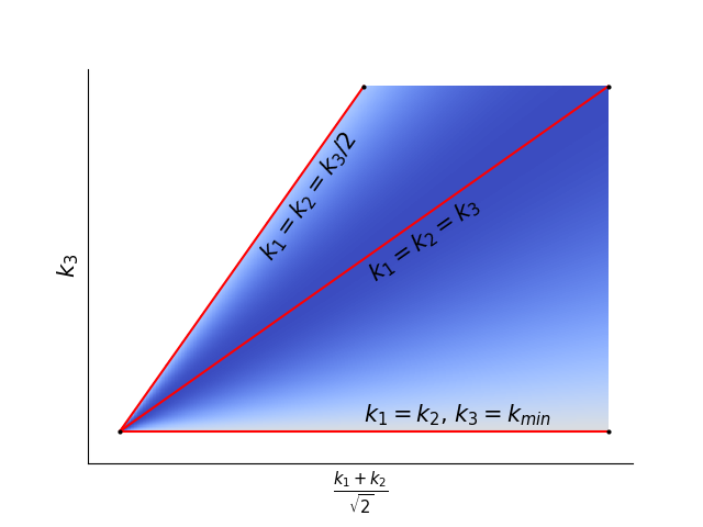
We display the phenomenology of our various validation examples by plotting slices through the tetrapyd, as detailed in figure 6. Along with the phenomenology plots we plot the residual (with respect to the totally converged result) on the same slice, relative to the magnitude of the shape (2.37). We emphasise that while these plots display slices through the tetrapyd, our actual result describes the shape function on the entire three-dimensional volume of the tetrapyd, and we measure our convergence over this whole space.
While one of the main advantages of this method is its direct link to the CMB, in this section we only concern ourselves with validating the code, not the observational viability of the scenarios considered. We focus on accurately and efficiently calculating the primordial tree-level comoving bispectrum, validating on models popular in the literature.
4.2 Quadratic slow-roll
The first model we will consider is slow-roll inflation on a quadratic potential (2.18). We consider two scenarios, both with . The first is deep in slow-roll, which we achieve by choosing ; then, choosing according to the slow-roll approximation, we get . We can then choose the initial value for to satisfy the Friedmann equation to sufficient precision. The second scenario is chosen to have a value for consistent with the Planck result, by choosing , so that . The shapes are shown in figure 7.
We choose the first scenario to have such a small value of so that we can use Maldacena’s shape (2.24) as a precision test. Indeed, we find that it has a scaled relative difference (2.36) of with this shape, contrasting a scaled relative difference of with the local template (2.26). This confirms that our methods and our implementation in code can accurately pick up this basic type of featureless non-Gaussianity.
For the second scenario, we cannot validate on Maldacena’s shape (2.24) or the local template (2.26), as for we only expect these templates to match the true result to percent level accuracy. Indeed, we find that our result has a correlation of with both (2.24) and (2.26), corresponding (in the sense of (2.36)) to a relative difference of , as expected. Instead, we validate this model using the squeezed limit test described above, verifying our result to .
This is a validation of the convergence of our basis, reaffirming the template decomposition results of figure 1 in the setting of the in-in formalism. It is also a stringent validation of our methods of including the higher-order coefficients, as insufficient care taken in the early-time sections of integrals (3.20), or in including the spatial derivatives from , could have easily swamped the result.


4.3 DBI inflation
Next, we show results for a similar pair of scenarios for DBI inflation. We choose with in (2.19) and (2.20). We choose , and then the starting condition for according to the slow-roll approximation, allowing us to choose such that the Friedmann equation is satisfied to sufficient precision. The first scenario is deep in slow-roll, with , while the second scenario saturates the Planck limit on , with . The resulting shapes are shown in figure 8.
The scenario deep in slow-roll has a error of relative to the DBI shape (2.27), and relative to the equilateral template (2.29). The second scenario has a relative error of with the scale-invariant DBI shape, and with the equilateral template. Including some scale dependence in the template, using (2.30), we get a relative error of . On the line defined by (4.1), both scenarios have a sub-percent difference from the consistency condition, with respect to the equilateral configurations, which decreases when configurations with a larger are considered.
Including the minimal information of an individual, approximately representative value of in allows us to converge to these smooth shapes quickly and robustly, overcoming the tetrapyd-vs-cube difficulties described in 3.1. Our accurate match to these shapes validates our implementation in code, and the ability of the method (and our basis in particular) to capture very different types of bispectrum shapes, local and equilateral.


4.4 Step features
Moving on from simple featureless bispectra, we present the results of our validation tests on non-Gaussianity coming from a sharp feature in the potential. We use the same parameters for the quadratic potential as in the second scenario in fig 7. In (2.21) we fix and (as with the second canonical quadratic example, ). Figure 9 shows results for the shape function for two step sizes, and . The resulting shape for small step sizes contains simple oscillations, linear in , whose phase is almost constant across the tetrapyd. When the step size is small, as expected, our result matches the analytic result of [5], presented there in equations (48), (54), (55). We plot a comparison of the result of [5] and our result in figure 11. For larger step size, we check the squeezed limit in figure 10, where we also show point tests against the PyTransport code. Across this range of step sizes, for the resulting shapes we obtain a full tetrapyd convergence test result (between and ) of between and and we verify the squeezed limit test to better than .
These examples show the utility of our methods in calculating bispectra with non-trivial shape and scale dependence, going beyond the simple examples of [20]. They validate the calculation of the high order coefficients, and show that our code as implemented can handle sharp deviations from slow-roll, generating non-Gaussianity around horizon crossing.


4.5 Resonance features
Now we further validate our code against two resonance models. In contrast to the previous sharp kink, this feature is extended, requiring precision at earlier times. The first, shown in figure 12, is a model with a canonical kinetic term, on a quadratic potential with a superimposed oscillation (2.22). We take , and . The resulting bispectrum has oscillations logarithmic in . In figure 12 we see the excellent agreement between our result and the PyTransport result, once initial conditions in both codes are set early enough to achieve convergence. This validates the code on non-Gaussianity generated deeper in the horizon. Note the change of phase in the squeezed limit, though this is expected to be unobservable. We obtain a full tetrapyd convergence test result (between and ) of , a squeezed limit test result of (along the line defined by (4.1)), and a relative difference of with respect to the PyTransport result, although this is only integrated over the two-dimensional slice presented in figure 12.
The time taken for the PyTransport code (per configuration) varies by a factor of around forty between the equilateral limit and the squeezed limit, as we show in figure 12. While the PyTransport code is extremely fast at calculating the shape function for a single -configuration, to obtain this two-dimensional slice through the tetrapyd took around seven hours; to obtain the shape function on the full three-dimensional tetrapyd would take much longer. In contrast, our code took less than an hour on the same machine to calculate the full shape function, not limited to the shown slice. The overall speed increase is, therefore, a factor on the order of to for the full shape information, speaking only on the level of primordial phenomenology, in addition to the advantage that our result is in a form designed to be compared with observation. We expect that our implementation can be optimised beyond this.
The second scenario we consider here also has an oscillation superimposed on its potential, but this time is a non-canonical model, the DBI model. The resulting bispectrum is shown in figure 13. Note especially the out-of-phase oscillations in the flattened limit, which are potentially observable. For the purpose of displaying this phenomenology, we place a window on the oscillation in the potential, smoothing out the resulting oscillations in the shape at low , to aid convergence. This validates our code on non-Gaussianity generated by deviations from Bunch-Davies behaviour [36, 30]. We obtain a convergence test result (between and ) of , and a squeezed limit test result of .


5 Discussion
In this work we have extended the modal methods of [17, 18, 19] to recast the calculation of the tree-level primordial bispectrum (2.8) into a form that explicitly preserves its separability. We emphasise again that this work has two main advantages over previous numerical methods. The more immediate is that by calculating the primordial bispectrum in terms of an expansion in some basis, the full bispectrum can be obtained much more efficiently than through repetitive integration separately for each -configuration. The second, more important, advantage is the link to observations. Unlike previous numerical and semi-analytic methods, once the shape function is expressed in some basis as in (2.2), the integral (2.7) and other computationally intensive steps involved in estimating a particular bispectrum in the CMB, can be precomputed. Since this large cost is only paid once per basis, once a basis which converges well for a broad range of models has been found, an extremely broad exploration of primordial bispectra becomes immediately feasible in the CMB. Making explicit the -dependence in this way also opens the door to vast increases in efficiency in connecting to other observables, by precomputation using the basis set, then performing a (relatively) cheap scan over inflation parameters.
Our work here goes beyond that of [20] in that our careful methodology allows us to accurately and efficiently go to much higher orders, in particular our methods of starting the time integrals (3.20) and of including the spatial derivative terms in the calculation. This allowed us to present this method for feature bispectra for the first time, demonstrating the efficient exploration of much more general primordial bispectrum phenomenology. We have also identified and addressed the effects of the non-physical -configurations on convergence within the three-dimensional tetrapyd. We explored, for the first time, possible basis set choices in the context of those effects. We showed rapid convergence on a broad range of scenarios, including cases with oscillatory features with non-trivial shape dependence, using our augmented Legendre polynomial basis, .
The immediate application of this work is the efficient exploration of bispectrum phenomenology, as our methods can much more quickly converge to the full shape information than previous numerical methods, which relied on calculating the shape function point-by-point, for each -configuration separately. We have implemented these methods for single field scenarios with a varying sound speed, scenarios which have a rich feature phenomenology. An important goal will be extending these methods to the case of multiple-field inflation.
The next immediate application will be to directly constrain parameters of inflationary scenarios through modal bispectrum results from the Planck satellite [10]. The details of the work required to directly connect our coefficients to the observed data, and the large but once-per-basis cost of this calculation, will be detailed in a forthcoming paper [21]. CMB and LSS data from forthcoming surveys will be able to use these separable primordial bispectra to even more precisely constrain the parameters of inflationary scenarios.
Acknowledgements.
We are grateful to Wuhyun Sohn and James Fergusson for enlightening discussions and useful comments. PC thanks the Robert Gardiner Memorial Scholarship and the Cambridge European Scholarship for their support, through the Cambridge Trust, as well as the UK STFC. PS acknowledges funding from STFC Consolidated Grant ST/P000673/1.References
- [1] J. Maldacena, Non-gaussian features of primordial fluctuations in single field inflationary models, Journal of High Energy Physics 5 (2003) 013 [astro-ph/0210603].
- [2] C. Burrage, R. H. Ribeiro and D. Seery, Large slow-roll corrections to the bispectrum of noncanonical inflation, Journal of Cosmology and Astro-Particle Physics 2011 (2011) 032 [1103.4126].
- [3] M. Alishahiha, E. Silverstein and D. Tong, DBI in the sky: Non-Gaussianity from inflation with a speed limit, Physical Review D 70 (2004) 123505 [hep-th/0404084].
- [4] C. T. Byrnes and K.-Y. Choi, Review of local non-gaussianity from multifield inflation, Advances in Astronomy 2010 (2010) 1–18.
- [5] P. Adshead, C. Dvorkin, W. Hu and E. A. Lim, Non-Gaussianity from step features in the inflationary potential, Physical Review D 85 (2012) 023531 [1110.3050].
- [6] R. Flauger and E. Pajer, Resonant Non-Gaussianity, JCAP 1101 (2011) 017 [1002.0833].
- [7] E. Komatsu, D. N. Spergel and B. D. Wandelt, Measuring primordial non-gaussianity in the cosmic microwave background, The Astrophysical Journal 634 (2005) 14–19.
- [8] M. Münchmeyer, F. Bouchet, M. G. Jackson and B. Wandelt, The komatsu spergel wandelt estimator for oscillations in the cosmic microwave background bispectrum, Astronomy & Astrophysics 570 (2014) A94.
- [9] Planck Collaboration, P. A. R. Ade, N. Aghanim, M. Arnaud, F. Arroja, M. Ashdown et al., Planck 2015 results. XVII. Constraints on primordial non-Gaussianity, Astronomy and Astrophysics 594 (2016) A17 [1502.01592].
- [10] P. Collaboration and Y. A. et al, Planck 2018 results. ix. constraints on primordial non-gaussianity, 1905.05697.
- [11] The Simons Observatory Collaboration, P. Ade, J. Aguirre, Z. Ahmed, S. Aiola, A. Ali et al., The Simons Observatory: Science goals and forecasts, ArXiv e-prints (2018) [1808.07445].
- [12] K. N. Abazajian, P. Adshead, Z. Ahmed, S. W. Allen, D. Alonso, K. S. Arnold et al., Cmb-s4 science book, first edition, 2016.
- [13] T. Baldauf, U. Seljak and L. Senatore, Primordial non-Gaussianity in the bispectrum of the halo density field, Journal of Cosmology and Astro-Particle Physics 2011 (2011) 006 [1011.1513].
- [14] D. Karagiannis, A. Lazanu, M. Liguori, A. Raccanelli, N. Bartolo and L. Verde, Constraining primordial non-Gaussianity with bispectrum and power spectrum from upcoming optical and radio surveys, Monthly Notices of the Royal Astronomical Society 478 (2018) 1341 [1801.09280].
- [15] X. Chen, C. Dvorkin, Z. Huang, M. H. Namjoo and L. Verde, The future of primordial features with large-scale structure surveys, Journal of Cosmology and Astroparticle Physics 11 (2016) 014 [1605.09365].
- [16] R. Scoccimarro, L. Hui, M. Manera and K. C. Chan, Large-scale bias and efficient generation of initial conditions for nonlocal primordial non-gaussianity, Physical Review D 85 (2012) .
- [17] J. R. Fergusson and E. P. S. Shellard, Primordial non-Gaussianity and the CMB bispectrum, Physical Review D 76 (2007) 083523 [astro-ph/0612713].
- [18] J. R. Fergusson and E. P. S. Shellard, Shape of primordial non-Gaussianity and the CMB bispectrum, Physical Review D 80 (2009) 043510 [0812.3413].
- [19] J. R. Fergusson, M. Liguori and E. P. S. Shellard, The CMB bispectrum, Journal of Cosmology and Astroparticle Physics 12 (2012) 032 [1006.1642].
- [20] H. Funakoshi and S. Renaux-Petel, A Modal Approach to the Numerical Calculation of Primordial non-Gaussianities, JCAP 1302 (2013) 002 [1211.3086].
- [21] W. Sohn and J. R. Fergusson, High-resolution CMB bispectrum estimator, (in preparation) .
- [22] A. Slosar, X. Chen, C. Dvorkin, D. Green, P. D. Meerburg, E. Silverstein et al., Scratches from the Past: Inflationary Archaeology through Features in the Power Spectrum of Primordial Fluctuations, arXiv e-prints (2019) arXiv:1903.09883 [1903.09883].
- [23] P. D. Meerburg and et al, Primordial Non-Gaussianity, arXiv e-prints (2019) arXiv:1903.04409 [1903.04409].
- [24] S. Weinberg, Quantum contributions to cosmological correlations, Phys. Rev. D 72 (2005) 043514 [hep-th/0506236].
- [25] S. Renaux-Petel, On the redundancy of operators and the bispectrum in the most general second-order scalar-tensor theory, Journal of Cosmology and Astro-Particle Physics 2012 (2012) 020 [1107.5020].
- [26] X. Chen, R. Easther and E. A. Lim, Large non-Gaussianities in single-field inflation, Journal of Cosmology and Astroparticle Physics 6 (2007) 023 [astro-ph/0611645].
- [27] X. Chen, R. Easther and E. A. Lim, Generation and Characterization of Large Non-Gaussianities in Single Field Inflation, Journal of Cosmology and Astroparticle Physics 0804 (2008) 010 [0801.3295].
- [28] X. Chen, M.-x. Huang, S. Kachru and G. Shiu, Observational signatures and non-Gaussianities of general single-field inflation, Journal of Cosmology and Astroparticle Physics 1 (2007) 002 [hep-th/0605045].
- [29] D. Seery and J. E. Lidsey, Primordial non-Gaussianities in single-field inflation, Journal of Cosmology and Astroparticle Physics 6 (2005) 003 [astro-ph/0503692].
- [30] N. Bartolo, D. Cannone and S. Matarrese, The effective field theory of inflation models with sharp features, Journal of Cosmology and Astro-Particle Physics 2013 (2013) 038 [1307.3483].
- [31] S. Passaglia and W. Hu, Scalar bispectrum beyond slow-roll in the unified EFT of inflation, Phys. Rev. D 98 (2018) 023526 [1804.07741].
- [32] P. Adshead, W. Hu and V. Miranda, Bispectrum in single-field inflation beyond slow-roll, Phys. Rev. D 88 (2013) 023507 [1303.7004].
- [33] V. Miranda, W. Hu and P. Adshead, Warp features in DBI inflation, Phys. Rev. D 86 (2012) 063529 [1207.2186].
- [34] E. Silverstein and D. Tong, Scalar speed limits and cosmology: Acceleration from D-cceleration, Phys. Rev. D 70 (2004) 103505 [hep-th/0310221].
- [35] V. Miranda and W. Hu, Inflationary steps in the Planck data, Phys. Rev. D 89 (2014) 083529 [1312.0946].
- [36] X. Chen, Folded resonant non-Gaussianity in general single field inflation, Journal of Cosmology and Astroparticle Physics 12 (2010) 003 [1008.2485].
- [37] S. Ávila, J. Martin and D. A. Steer, Superimposed oscillations in brane inflation, Journal of Cosmology and Astro-Particle Physics 2014 (2014) 032 [1304.3262].
- [38] S. Garcia-Saenz, S. Renaux-Petel and J. Ronayne, Primordial fluctuations and non-Gaussianities in sidetracked inflation, ArXiv e-prints (2018) [1804.11279].
- [39] J. Garriga and V. F. Mukhanov, Perturbations in k-inflation, Physics Letters B 458 (1999) 219 [hep-th/9904176].
- [40] G. Cabass, E. Pajer and F. Schmidt, How Gaussian can our Universe be?, JCAP 1701 (2017) 003 [1612.00033].
- [41] M. Münchmeyer, P. D. Meerburg and B. D. Wandelt, Optimal estimator for resonance bispectra in the CMB, Phys. Rev. D 91 (2015) 043534 [1412.3461].
- [42] D. K. Hazra, L. Sriramkumar and J. Martin, BINGO: a code for the efficient computation of the scalar bi-spectrum, Journal of Cosmology and Astroparticle Physics 5 (2013) 026 [1201.0926].
- [43] J. S. Horner and C. R. Contaldi, Non-Gaussianity Unleashed, ArXiv e-prints (2013) [1303.2119].
- [44] J. S. Horner and C. R. Contaldi, Non-gaussian signatures of general inflationary trajectories, Journal of Cosmology and Astroparticle Physics 9 (2014) 001 [1311.3224].
- [45] J. S. Horner and C. R. Contaldi, The bispectrum of single-field inflationary trajectories with , ArXiv e-prints (2015) [1503.08103].
- [46] M. Dias, J. Frazer, D. J. Mulryne and D. Seery, Numerical evaluation of the bispectrum in multiple field inflation—the transport approach with code, JCAP 1612 (2016) 033 [1609.00379].
- [47] D. J. Mulryne and J. W. Ronayne, PyTransport: A Python package for the calculation of inflationary correlation functions, ArXiv e-prints (2016) [1609.00381].
- [48] J. W. Ronayne and D. J. Mulryne, Numerically evaluating the bispectrum in curved field-space— with PyTransport 2.0, JCAP 1801 (2018) 023 [1708.07130].
- [49] S. Butchers and D. Seery, Numerical evaluation of inflationary 3-point functions on curved field space, ArXiv e-prints (2018) [1803.10563].
- [50] J. Hung, J. R. Fergusson and E. P. S. Shellard, Advancing the matter bispectrum estimation of large-scale structure: a comparison of dark matter codes, arXiv e-prints (2019) [1902.01830].
- [51] P. Creminelli and M. Zaldarriaga, A single-field consistency relation for the three-point function, Journal of Cosmology and Astroparticle Physics 10 (2004) 006 [astro-ph/0407059].
- [52] P. Creminelli, G. D’Amico, M. Musso and J. Noreña, The (not so) squeezed limit of the primordial 3-point function, Journal of Cosmology and Astroparticle Physics 11 (2011) 038 [1106.1462].
- [53] N. Arkani-Hamed, D. Baumann, H. Lee and G. L. Pimentel, The Cosmological Bootstrap: Inflationary Correlators from Symmetries and Singularities, JHEP 04 (2020) 105 [1811.00024].
- [54] F. Arroja and T. Tanaka, A note on the role of the boundary terms for the non-Gaussianity in general k-inflation, Journal of Cosmology and Astro-Particle Physics 2011 (2011) 005 [1103.1102].
- [55] G. Rigopoulos, Gauge invariance and non-Gaussianity in inflation, Phys. Rev. D 84 (2011) 021301 [1104.0292].
- [56] A. Dixit, L. Jiu, V. H. Moll and C. Vignat, The finite Fourier transform of classical polynomials, ArXiv e-prints (2014) [1402.5544].
- [57] A. Iserles and S. P. Norsett, Efficient quadrature of highly efficient integrals using deriatives, Royal Society Publishing, Volume 461, Issue 2057 (2005) .