跳到论文正文
W Papers独立论文阅读器 arXiv:2012.08541 论文正文 计算阅读时间 · 0%
引用这篇论文根据当前论文元数据生成,正式投稿前建议核对。


License: CC BY 4.0
arXiv:2012.08541v2 [cond-mat.soft] 20 Jul 2021

Long-range correlations in pinned athermal networks

Debankur Das Email: debankurd@tifrh.res.in Affiliation: Centre for Interdisciplinary Sciences, Tata Institute of Fundamental Research, Hyderabad 500107, India    Pappu Acharya Email: pappuacharya@tifrh.res.in Affiliation: Centre for Interdisciplinary Sciences, Tata Institute of Fundamental Research, Hyderabad 500107, India    Kabir Ramola Email: kramola@tifrh.res.in Affiliation: Centre for Interdisciplinary Sciences, Tata Institute of Fundamental Research, Hyderabad 500107, India
August 11, 2026
Abstract

We derive exact results for displacement fields that develop as a response to external pinning forces in two dimensional athermal networks. For a triangular lattice arrangement of particles interacting through soft potentials, we develop a Green’s function formalism which we use to derive exact results for displacement fields produced by localized external forces. We show that in the continuum limit the displacement fields decay as 1/r1/r at large distances rr away from a force dipole. Finally, we extend our formulation to study correlations in the displacement fields produced by the external pinning forces. We show that uncorrelated pinned forces at each vertex give rise to long-range correlations in displacements in athermal systems, with a non-trivial system size dependence. We verify our predictions with numerical simulations of athermal networks in two dimensions.

I Introduction

Networks composed of athermal constituents such as jammed particles arise in a variety of contexts O’Hern et al. 2003, including in granular Behringer and Chakraborty 2018; Goldenberg and Goldhirsch 2002 and glassy systems Ikeda et al. 2012, active matter Henkes et al. 2011, as well as biological tissues Bi et al. 2016; Broedersz et al. 2011; Boromand et al. 2018. Such materials are robust to thermal agitations and differ from thermal systems in their response to external perturbations, as well as fluctuations in positions and forces Acharya et al. 2020. The response of athermal materials to external perturbations has many industrial as well as biological applications Cates et al. 1998; Head et al. 2005; Athanassiadis et al. 2014; Ramola and Chakraborty 2017; Bouchaud et al. 2002; Geng et al. 2001, and continues to be the subject of active research. Similarly, athermal systems driven by local active forces arise in various contexts in physics and biology Janeš et al. 2019a; Janeš et al. 2019b; Ronceray et al. 2016; Ronceray et al. 2019; Schwarz and Safran 2013. Although many properties of athermal systems have been extensively studied over the last few decades, the fluctuations in displacement fields, as well as the long-range correlations that develop in such systems, are relatively less well understood Bi et al. 2015; DeGiuli 2018; Lemaître 2014; Lemaître et al. 2021; Chikkadi et al. 2011. Developing theories for the collective behaviour of athermal systems in the presence of external forces such as gravity or active internal forces therefore represents a new challenge Kadanoff 1999; de Gennes 1999.

The quasi-static response of athermal materials to local pinning forces is also important in the study of granular materials as well as glasses Bhowmik et al. 2019; Zeng et al. 1999; Lerner and Bouchbinder 2018, where local force perturbations can be used to extract lengthscales Rainone et al. 2020. In such systems, the constraints of mechanical equilibrium alone do not provide enough equations to solve for the stress tensor, which can lead to non-trivial stress transmission properties Liu et al. 1995; Nampoothiri et al. 2020. Although theories of continuum elasticity posit constitutive relations between the microscopic stress and strain fields, it is as yet unclear how such relationships emerge at large lengthscales in disordered athermal materials. For example, the continuum equations that emerge can be elliptic, or hyperbolic Bouchaud 2002, depending on the nature of the underlying medium, but a clear understanding of this phenomenon is still lacking. Moreover, predicting fluctuations and correlations in athermal ensembles remains a challenging theoretical task. In this context it is useful to appeal to systems where the strain field can be computed exactly to determine the nature of the correlations and response in athermal systems .

Figure 1: The displacement response of an athermal membrane composed of soft particles to the presence of active (external) forces imposed on each site (depicted with arrows). The particles are colored according to their displacements from the crystalline positions along the xx-direction. The external forces are drawn from uncorrelated underlying distributions. The displacements of the sites from their crystalline positions as a response, displaying large correlated regions. The separation between the particles in the initial crystalline state is R0=1.2R_{0}=1.2, and the equilibrium bond lengths are Lrest=1.1L_{\text{rest}}=1.1.

The stress response of triangular networks with microscopic force balance constraints has been a paradigmatic model of stress transmission in granular systems Liu et al. 1995; Snoeijer and Van Leeuwen 2002; Radjai 2015, and has been used to model continuum athermal elasticity at large lengthscales Otto et al. 2003. However, incorporating the effects of microscopic disorder, such as in the external forces, within an exact framework has remained difficult owing to the non-trivial spatial arrangements of particles in minimum energy configurations. In this context it is important to appeal to systems where exact results can be obtained. In this paper we present exact results for displacement fields and their correlations in athermal networks using a model of frictionless soft particles in an initial triangular lattice arrangement. Our exact results demonstrate that in the athermal systems where mechanical equilibrium is exactly imposed at the local level, uncorrelated external forces can give rise to large correlated regions in the system. Indeed, as we show, in addition to being long-ranged, the displacement correlations have a non-trivial system size dependence.

II Pinned Network Model

We study a system of equal-sized particles with initial positions {r→i,0}≡{xi,0,yi,0}\{\vec{r}_{i,0}\}\equiv\{x_{i,0},y_{i,0}\}, arranged in an L×LL\times L triangular lattice with lattice constant R0R_{0}. We impose periodic boundary conditions in both the xx and yy directions. Each particle interacts with its nearest neighbours through a distance dependent force law. We consider these interactions to be harmonic, with a spring constant KK and an equilibrium bond length LrestL_{\text{rest}}. Our results can be easily generalized to other types of interactions as well. The Hamiltonian of the system is given by

ℋ=∑i=1L2pi22​mi+K2​∑i=1L2∑⟨i​j⟩(|r→i−r→j|−Lrest)2,\mathcal{H}=\sum_{i=1}^{L^{2}}\frac{p_{i}^{2}}{2m_{i}}+\frac{K}{2}\sum_{i=1}^{L^{2}}\sum_{\langle ij\rangle}(|\vec{r}_{i}-\vec{r}_{j}|-L_{\text{rest}})^{2}, (1)

where mim_{i} is the mass and r→i\vec{r}_{i} represents the instantaneous position of the ithi^{\text{th}} particle. The brackets ⟨⟩\langle\rangle in the above summation denote nearest-neighbours on the triangular lattice network with j>ij>i. We define R0=Lrest​(1+α)R_{0}=L_{\text{rest}}(1+\alpha), where α\alpha quantifies the compression of the initial crystalline state. When α<0\alpha<0 the system is overcompressed and the forces between the vertices (particles) are repulsive, whereas when α>0\alpha>0 the system is under-compressed and the forces are attractive. We consider the athermal version of this system, i.e. the zero temperature limit in which the momentum term in Eq. (1) is irrelevant, and we only deal with the minimum of the potential energy. In addition to the inter-particle forces, we impose forces f→i,ext\vec{f}_{i,\text{ext}} at every vertex ii that represent the external pinning forces acting on the system. We display a typical force balanced configuration of such a network in the presence of random pinning forces in Fig. 1.

III Simulation Details

In order to verify that the predictions from our theory are able to capture the non-trivial nature of the response in such systems, we simulate the athermal triangular network in the presence of external forces. We consider an ideal triangular lattice with lattice parameter R0≠LrestR_{0}\neq L_{\text{rest}}. At every vertex ii, we impose an external force f→i,ext\vec{f}_{i,\text{ext}}. We consider force balanced configurations, i.e. configurations at energy minima. We minimize the energy of the system using the FIRE (Fast Inertial Relaxation Engine) algorithm Bitzek et al. 2006, which can naturally incorporate externally imposed forces. The implementation of the algorithm is simple and rapidly leads to a minimum energy configuration. At every time step we compute the power P=F→.v→P=\vec{F}.\vec{v} in the entire system. If P>0P>0, the velocity is set to v→→(1−β)​v→+β​F^​|v→|\vec{v}\to(1-\beta)\vec{v}+\beta\hat{F}|\vec{v}|, the time step is increased as Δ​t=Δ​t​finc\Delta t=\Delta tf_{\text{inc}}, up to the maximum value Δ​t=Δ​tmax\Delta t=\Delta t_{\text{max}} and β\beta is changed to β​fβ\beta f_{\beta}. If P<0P<0, the velocity is set to zero, the time step is decreased Δ​t=Δ​t​fdec\Delta t=\Delta tf_{\text{dec}} and β\beta is reset back to its initial value βstart\beta_{\text{start}}. In our simulations, we use β=βstart=0.01\beta=\beta_{\text{start}}=0.01, Δ​t=0.0001\Delta t=0.0001, Δ​tmax=0.001\Delta t_{\text{max}}=0.001, fβ=0.99f_{\beta}=0.99, finc=1.1f_{\text{inc}}=1.1, and fdec=0.5f_{\text{dec}}=0.5.

IV Linearized Force Balance

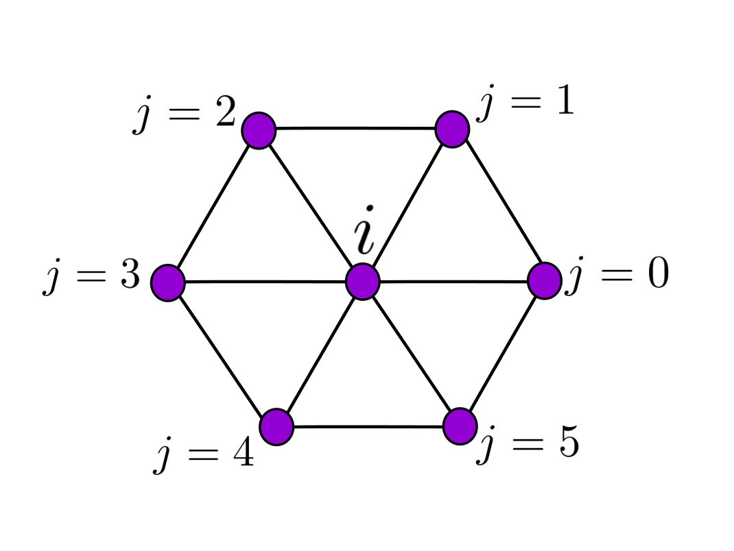
Refer to caption
Figure 2: The labeling convention used in our computation. The six neighbours of every node ii of the lattice are labeled j=0j=0 to 55. The angles of the bonds between nodes in the reference crystalline state can take any of six values (depending on jj) with the positive xx-axis, θi​j=2​π​j/6.\theta_{ij}=2\pi j/6.

We begin by analyzing the response of the ideal triangular lattice in the limit of weak external forces. The inter-particle forces are determined from Eq. (1) and are given by

fi​jx=−K⁡(xi​j2+yi​j2−Lrest)​xi​jri​j,fi​jy=−K⁡(xi​j2+yi​j2−Lrest)​yi​jri​j.\begin{split}f_{ij}^{x}=-K\left(\sqrt{x_{ij}^{2}+y_{ij}^{2}}-L_{\text{rest}}\right)\frac{x_{ij}}{r_{ij}},\\ f_{ij}^{y}=-K\left(\sqrt{x_{ij}^{2}+y_{ij}^{2}}-L_{\text{rest}}\right)\frac{y_{ij}}{r_{ij}}.\end{split} (2)

Here fi​jx⁡(y)f_{ij}^{x(y)} are the x⁡(y)x(y) components of the force between nodes ii and jj and xi​j=xj−xix_{ij}=x_{j}-x_{i} represents the distance between particles ii and jj. The ground state of the system is determined by the condition of mechanical equilibrium, i.e. each site is in force balance with

∑j=05fi​jx+fi,extx=0,∑j=05fi​jy+fi,exty=0,∀i,\sum_{j=0}^{5}f_{ij}^{x}+{f}_{i,\text{ext}}^{x}=0,~~~~~\sum_{j=0}^{5}f_{ij}^{y}+{f}_{i,\text{ext}}^{y}=0,~~~~~\forall~i, (3)

where the sum includes the six neighbours j=0j=0 to 55 of the it​hi^{th} site (Fig. 2). In addition to the above force balance equations at every site, we also impose global force balance on the system with

∑i=1L2fi,extx=0,∑i=1L2fi,exty=0.\sum_{i=1}^{L^{2}}{f}_{i,\text{ext}}^{x}=0,~~~~~\sum_{i=1}^{L^{2}}{f}_{i,\text{ext}}^{y}=0. (4)

In the absence of external forces, the ground state configuration is the unperturbed triangular lattice with particle positions {r→i,0}\{\vec{r}_{i,0}\}. We next treat the introduction of external forces as a perturbation. As a response to this perturbation, the positions of the vertices change as

xi\displaystyle x_{i} =\displaystyle= xi,0+δ​xi,\displaystyle x_{i,0}+\delta x_{i},
yi\displaystyle y_{i} =\displaystyle= yi,0+δ​yi.\displaystyle y_{i,0}+\delta y_{i}. (5)

Here δ​xi\delta x_{i} and δ​yi\delta y_{i} are the xx and yy displacements of the it​hi^{th} site from their positions in the initial triangular lattice. The force law in Eq. (2) is a non-linear function of the inter-particle distances xi​jx_{ij} and yi​jy_{ij}. In the limit of small perturbations, we can expand Eq. (2) up to linear order in the relative displacements δ​x​(y)i​j=δ​x​(y)j−δ​x​(y)i\delta x(y)_{ij}=\delta x(y)_{j}-\delta x(y)_{i}, leading to

δ​fi​jx=Ci​jx​x​δ​xi​j+Ci​jx​y​δ​yi​j,δ​fi​jy=Ci​jy​x​δ​xi​j+Ci​jy​y​δ​yi​j.\begin{split}\delta f_{ij}^{x}=C_{ij}^{xx}\delta x_{ij}+C_{ij}^{xy}\delta y_{ij},\\ \delta f_{ij}^{y}=C_{ij}^{yx}\delta x_{ij}+C_{ij}^{yy}\delta y_{ij}.\end{split} (6)

Without loss of generality we may set K=1K=1. The linear coefficients Ci​jμ​νC_{ij}^{\mu\nu} are then given by

Ci​jx​x\displaystyle C_{ij}^{xx} =\displaystyle= −2​R0+Lrest−Lrest​cos⁡(2​j​π3)2​R0,\displaystyle\frac{-2R_{0}+L_{\text{rest}}-L_{\text{rest}}\cos(\frac{2j\pi}{3})}{2R_{0}},
Ci​jx​y\displaystyle C_{ij}^{xy} =\displaystyle= −Lrest​sin⁡(2​j​π3)2​R0,\displaystyle-\frac{L_{\text{rest}}\sin(\frac{2j\pi}{3})}{2R_{0}},
Ci​jy​x\displaystyle C_{ij}^{yx} =\displaystyle= −Lrest​sin⁡(2​j​π3)2​R0,\displaystyle-\frac{L_{\text{rest}}\sin(\frac{2j\pi}{3})}{2R_{0}},
Ci​jy​y\displaystyle C_{ij}^{yy} =\displaystyle= −2​R0+Lrest+Lrest​cos⁡(2​j​π3)2​R0.\displaystyle\frac{-2R_{0}+L_{\text{rest}}+L_{\text{rest}}\cos(\frac{2j\pi}{3})}{2R_{0}}. (7)

We note that the coefficients Ci​jμ​νC_{ij}^{\mu\nu} represent the elements of the Hessian matrix of the crystalline system. Crucially, these coefficients Ci​jμ​νC^{\mu\nu}_{ij}, being drawn from the unperturbed crystalline arrangement are translationally invariant, i.e. they do not depend on the site index ii. Next, using these linearized expressions we can relate the changes in positions to the external forces as

∑j=05Ci​jx​x​(δ​xj−δ​xi)+∑j=05Ci​jx​y​(δ​yj−δ​yi)=−fi,extx,\displaystyle\sum_{j=0}^{5}C_{ij}^{xx}(\delta x_{j}-\delta x_{i})+\sum_{j=0}^{5}C_{ij}^{xy}(\delta y_{j}-\delta y_{i})=-f_{i,\text{ext}}^{x}, (8)
∑j=05Ci​jy​x​(δ​xj−δ​xi)+∑j=05Ci​jy​y​(δ​yj−δ​yi)=−fi,exty.\displaystyle\sum_{j=0}^{5}C_{ij}^{yx}(\delta x_{j}-\delta x_{i})+\sum_{j=0}^{5}C_{ij}^{yy}(\delta y_{j}-\delta y_{i})=-f_{i,\text{ext}}^{y}.

These translationally invariant equations of force balance can be simplified in Fourier space. In order to define a Fourier transform we assign the displacement field (δ​xi,δ​yi)≡(δ​x​(r→),δ​y​(r→))(\delta x_{i},\delta y_{i})\equiv(\delta x(\vec{r}),\delta y(\vec{r})) to every site ii at the unperturbed lattice positions r→≡r→i,0\vec{r}\equiv\vec{r}_{i,0}. The Fourier transform of the displacements is δx~(y~)(k→)=∑r→exp(ik→.r→)δx(y)(r→)\delta\tilde{x}(\tilde{y})(\vec{k})=\sum_{\vec{r}}\exp(i\vec{k}.\vec{r})\delta x(y)(\vec{r}) and external forces is f~extx⁡(y)(k→)=∑r→exp(ik→.r→)fi,extx⁡(y){\tilde{f}}^{x(y)}_{\text{ext}}(\vec{k})=\sum_{\vec{r}}\exp(i\vec{k}.\vec{r})f_{i,\text{ext}}^{x(y)}. Here k→=(kx,ky)≡(2​π​l2​L,2​π​mL)\vec{k}=(k_{x},k_{y})\equiv\Big(\frac{2\pi l}{2L},\frac{2\pi m}{L}\Big) are the reciprocal lattice vectors of the triangular lattice and the volume of the system is V=2​L2V=2L^{2} Horiguchi 1972. It is also convenient to define the basic translation coefficients in Fourier space (see Supplemental Material for details  sup)

ℱj​(k→)\displaystyle\mathcal{F}_{j}(\vec{k}) =\displaystyle= exp(−ik→.𝕣→j),\displaystyle\exp(-i\vec{k}.\vec{\mathbb{r}}_{j}), (9)

where 𝕣→j\vec{\mathbb{r}}_{j} represent the lattice translation vectors given by 𝕣→0=(2,0)\vec{\mathbb{r}}_{0}=(2,0), 𝕣→1=(1,1)\vec{\mathbb{r}}_{1}=(1,1), 𝕣→2=(−1,1)\vec{\mathbb{r}}_{2}=(-1,1), 𝕣→3=(−2,0)\vec{\mathbb{r}}_{3}=(-2,0), 𝕣→4=(−1,−1)\vec{\mathbb{r}}_{4}=(-1,-1), 𝕣→5=(1,−1)\vec{\mathbb{r}}_{5}=(1,-1). Next, multiplying Eq. (8) by exp(ik→.r→)\exp(i\vec{k}.\vec{r}) and summing over all sites of the lattice, we arrive at the following matrix equation at each reciprocal lattice point

(Ax​x​(k→)Ax​y​(k→)Ay​x​(k→)Ay​y​(k→))​(δ​x~​(k→)δ​y~​(k→))=(−f~extx​(k→)−f~exty​(k→)).\left(\begin{matrix}A^{xx}(\vec{k})&A^{xy}(\vec{k})\\ A^{yx}(\vec{k})&A^{yy}(\vec{k})\end{matrix}\right)\left(\begin{matrix}\delta\tilde{x}(\vec{k})\\ \delta\tilde{y}(\vec{k})\end{matrix}\right)=\left(\begin{matrix}{-\tilde{f}}^{x}_{\text{ext}}(\vec{k})\\ {-\tilde{f}}^{y}_{\text{ext}}(\vec{k})\end{matrix}\right). (10)

The above matrix elements Aμ​νA^{\mu\nu} can be expressed in terms of the coefficients Ci​jμ​νC_{ij}^{\mu\nu} as

Ax​x​(k→)\displaystyle A^{xx}(\vec{k}) =\displaystyle= −∑j=05(1−ℱj(k→))Ci​jx​x,\displaystyle-\sum_{j=0}^{5}(1-\mathcal{F}_{j}(\vec{k}))C^{xx}_{ij},
Ax​y​(k→)\displaystyle A^{xy}(\vec{k}) =\displaystyle= −∑j=05(1−ℱj(k→))Ci​jx​y,\displaystyle-\sum_{j=0}^{5}(1-\mathcal{F}_{j}(\vec{k}))C^{xy}_{ij},
Ay​x​(k→)\displaystyle A^{yx}(\vec{k}) =\displaystyle= −∑j=05(1−ℱj(k→))Ci​jy​x,\displaystyle-\sum_{j=0}^{5}(1-\mathcal{F}_{j}(\vec{k}))C^{yx}_{ij},
Ay​y​(k→)\displaystyle A^{yy}(\vec{k}) =\displaystyle= −∑j=05(1−ℱj(k→))Ci​jy​y.\displaystyle-\sum_{j=0}^{5}(1-\mathcal{F}_{j}(\vec{k}))C^{yy}_{ij}. (11)

The solution for the displacements in Fourier space in response to externally imposed forces can then be obtained by solving Eq. (10).

V Response Green’s Functions

We can interpret the matrix elements of A−1A^{-1} as Green’s functions in Fourier space as

G=A−1=(G~x​x​(k→)G~x​y​(k→)G~y​x​(k→)G~y​y​(k→)).G=A^{-1}=\left(\begin{matrix}\tilde{G}_{xx}(\vec{k})&\tilde{G}_{xy}(\vec{k})\\ \tilde{G}_{yx}(\vec{k})&\tilde{G}_{yy}(\vec{k})\end{matrix}\right). (12)

These Green’s functions can then be used to derive the Fourier transformed displacements as

δ​x~​(k→)\displaystyle\delta\tilde{x}(\vec{k}) =\displaystyle= −G~x​x​(k→)​f~extx​(k→)−G~x​y​(k→)​f~exty​(k→),\displaystyle-\tilde{G}_{xx}(\vec{k})\tilde{f}^{x}_{\text{ext}}(\vec{k})-\tilde{G}_{xy}(\vec{k})\tilde{f}^{y}_{\text{ext}}(\vec{k}),
δ​y~​(k→)\displaystyle\delta\tilde{y}(\vec{k}) =\displaystyle= −G~y​x​(k→)​f~extx​(k→)−G~y​y​(k→)​f~exty​(k→).\displaystyle-\tilde{G}_{yx}(\vec{k})\tilde{f}^{x}_{\text{ext}}(\vec{k})-\tilde{G}_{yy}(\vec{k})\tilde{f}^{y}_{\text{ext}}(\vec{k}). (13)

The external forces therefore play the role of a source term that generate the displacement fields at every site. In order to obtain the actual displacements up to linear order, we perform an inverse Fourier transform of Eq. (13). Defining the Green’s function in real space r→=(x,y)\vec{r}=(x,y) as

Gμ​ν(r→)=1V∑l=02​L−1∑m=0L−1e−ik→⋅r→G~μ​ν(k→),G_{\mu\nu}(\vec{r})=\frac{1}{V}\sum_{l=0}^{2L-1}\sum_{m=0}^{L-1}e^{-i\vec{k}\cdot\vec{r}}\tilde{G}_{\mu\nu}(\vec{k}), (14)

we arrive at the following form of the displacement field in real space

δx(r→)=−∑r→′[Gx​x(r→−r→′)δfxext(r→′)+Gx​y(r→−r→′)δfyext(r→′)],\displaystyle\delta x(\vec{r})=-\sum_{\vec{r}^{\prime}}\left[G_{xx}(\vec{r}-\vec{r}^{\prime})\delta f^{x}_{\text{ext}}(\vec{r}^{\prime})+G_{xy}(\vec{r}-\vec{r}^{\prime})\delta f^{y}_{\text{ext}}(\vec{r}^{\prime})\right], (15)
δy(r→)=−∑r→′[Gy​x(r→−r→′)δfxext(r→′)+Gy​y(r→−r→′)δfyext(r→′)].\displaystyle\delta y(\vec{r})=-\sum_{\vec{r}^{\prime}}\left[G_{yx}(\vec{r}-\vec{r}^{\prime})\delta f^{x}_{\text{ext}}(\vec{r}^{\prime})+G_{yy}(\vec{r}-\vec{r}^{\prime})\delta f^{y}_{\text{ext}}(\vec{r}^{\prime})\right].

The advantage of our technique can be described as follows. There are two constraint equations at each vertex corresponding to forces in the xx and yy directions. Therefore, in order to solve for the displacements of the L2L^{2} vertices in the xx and yy directions, one needs to simultaneously solve the 2​L22L^{2} constraint equations. A Fourier transform reduces the problem to an inversion of a 2×22\times 2 matrix at each reciprocal lattice point k→\vec{k}.

As mentioned above, the elements of the matrix A−1\text{A}^{-1} in Eq. (12) can be interpreted as the Green’s function of the response to a point charge in Fourier space. To obtain simplified expressions for these Green’s functions, it is convenient to define the following quantities

Γ1​(kx,ky,α)\displaystyle\Gamma_{1}(k_{x},k_{y},\alpha) =\displaystyle= −3−6​α+2​α​cos⁡(2​kx)\displaystyle-3-6\alpha+2\alpha\cos(2k_{x})
+(3+4​α)​cos⁡(kx)​cos⁡(ky),\displaystyle+(3+4\alpha)\cos(k_{x})\cos(k_{y}),
Γ2​(kx,ky,α)\displaystyle\Gamma_{2}(k_{x},k_{y},\alpha) =\displaystyle= −3−6​α+2​(1+α)​cos⁡(2​kx)\displaystyle-3-6\alpha+2(1+\alpha)\cos(2k_{x})
+(1+4​α)​cos⁡(kx)​cos⁡(ky),\displaystyle+(1+4\alpha)\cos(k_{x})\cos(k_{y}),
η⁡(kx,ky,α)\displaystyle\eta(k_{x},k_{y},\alpha) =\displaystyle= 3​sin⁡(kx)​sin⁡(ky).\displaystyle\sqrt{3}\sin(k_{x})\sin(k_{y}). (16)

Here α\alpha represents the compression in the system, with lattice constant of the crystalline system given by R0=Lrest​(1+α)R_{0}=L_{\text{rest}}(1+\alpha). In terms of the above functions, the expressions for the Green’s functions simplify to

G~x​x​(kx,ky,α)\displaystyle\tilde{G}_{xx}(k_{x},k_{y},\alpha) =\displaystyle= −(1+α)​Γ1(Γ1​Γ2)−η2,\displaystyle-(1+\alpha)\frac{\Gamma_{1}}{(\Gamma_{1}\Gamma_{2})-{\eta}^{2}},
G~x​y​(kx,ky,α)\displaystyle\tilde{G}_{xy}(k_{x},k_{y},\alpha) =\displaystyle= −(1+α)​η(Γ1​Γ2)−η2,\displaystyle-(1+\alpha)\frac{\eta}{(\Gamma_{1}\Gamma_{2})-{\eta}^{2}},
G~y​x​(kx,ky,α)\displaystyle\tilde{G}_{yx}(k_{x},k_{y},\alpha) =\displaystyle= −(1+α)​η(Γ1​Γ2)−η2,\displaystyle-(1+\alpha)\frac{\eta}{(\Gamma_{1}\Gamma_{2})-{\eta}^{2}},
G~y​y​(kx,ky,α)\displaystyle\tilde{G}_{yy}(k_{x},k_{y},\alpha) =\displaystyle= −(1+α)​Γ2(Γ1​Γ2)−η2.\displaystyle-(1+\alpha)\frac{\Gamma_{2}}{(\Gamma_{1}\Gamma_{2})-{\eta}^{2}}. (17)
Refer to caption
Figure 3: The Green’s functions of the response G~μ​ν​(k→)\tilde{G}_{\mu\nu}(\vec{k}) in Fourier space k→≡(kx,ky)≡(k​cos⁡(ψ),k​sin⁡(ψ))\vec{k}\equiv(k_{x},k_{y})\equiv(k\cos(\psi),k\sin(\psi)). (a) G~x​x​(k→)\tilde{G}_{xx}(\vec{k}) (b) G~x​y​(k→)\tilde{G}_{xy}(\vec{k})(c) G~y​y​(k→)\tilde{G}_{yy}(\vec{k}). Note that the limits are different along different angles ψ\psi as k→0k\to 0. (d) All Green’s functions display a ∼1/k2\sim 1/k^{2} behaviour at small kk.

V.1 Continuum Green’s Functions

We next use the framework developed above to derive the continuum behaviour of this system. To obtain the behaviour at large distances rr, we analyze these expressions at small values of kk. In the limit k→0k\to 0, we obtain the following expression for the Green’s functions in Fourier space, with (kx,ky)≡(k​cos⁡(ψ),k​sin⁡(ψ))(k_{x},k_{y})\equiv(k\cos(\psi),k\sin(\psi))

G~x​x​(k,ψ)\displaystyle\tilde{G}_{xx}(k,\psi) =\displaystyle= −1k2​(2+2​α)​(3+8​α+4​α​cos⁡(2​ψ))(3+16​α+16​α2)​(2+cos⁡(2​ψ))2,\displaystyle-\frac{1}{k^{2}}\frac{(2+2\alpha)(3+8\alpha+4\alpha\cos(2\psi))}{(3+16\alpha+16\alpha^{2})(2+\cos(2\psi))^{2}},
G~x​y​(k,ψ)\displaystyle\tilde{G}_{xy}(k,\psi) =\displaystyle= −1k2​2​3​(1+α)​(sin⁡(2​ψ))(3+16​α+16​α2)​(2+cos⁡(2​ψ))2,\displaystyle-\frac{1}{k^{2}}\frac{2\sqrt{3}(1+\alpha)(\sin(2\psi))}{(3+16\alpha+16\alpha^{2})(2+\cos(2\psi))^{2}},
G~y​y​(k,ψ)\displaystyle\tilde{G}_{yy}(k,\psi) =\displaystyle= −1k2​(2+2​α)​(5+8​α+4​(1+α)​cos⁡(2​ψ))(3+16​α+16​α2)​(2+cos⁡(2​ψ))2.\displaystyle-\frac{1}{k^{2}}\frac{(2+2\alpha)(5+8\alpha+4(1+\alpha)\cos(2\psi))}{(3+16\alpha+16\alpha^{2})(2+\cos(2\psi))^{2}}.

The transverse Green’s functions of the response are equal with G~y​x​(k→)=G~x​y​(k→)\tilde{G}_{yx}(\vec{k})=\tilde{G}_{xy}(\vec{k}). We note that all the Green’s functions display a ∼1/k2\sim 1/k^{2} behaviour at small kk. Therefore, in the small kk limit we have G~μ​ν​(k,ψ)=g~μ​ν​(ψ)/k2\tilde{G}_{\mu\nu}(k,\psi)=\tilde{g}_{\mu\nu}(\psi)/k^{2}, where g~μ​ν​(ψ)\tilde{g}_{\mu\nu}(\psi) encodes the angular dependence of these functions. The above expressions make it clear that the response of the medium has a non-trivial dependence on the compression α\alpha. In Fig. 3 we plot these Green’s functions in Fourier space, for small values of kk. We note that the expressions in Eq. () have different limits as k→0k\to 0 along different directions. Such singularities are linked to the tensorial nature of the mechanical equilibrium constraints governing the stress tensor Nampoothiri et al. 2020.

V.2 Green’s Functions in Real Space

Refer to caption
Figure 4: Plots of (a) the displacements of each particle along the xx-direction produced by a force dipole obtained from simulations (b) xx-displacements from theory (c) difference in xx-displacements from theory and simulations. (d) The displacements along the yy-direction obtained from simulations (e) yy-displacements from theory (f) difference in yy-displacements from theory and simulations. The external forces are placed on adjacent sites at the origin, with an orientation along the xx-direction (ϕ=0\phi=0). The magnitude of the force dipole is f0f_{0} =0.005.

We next study the Green’s function in real space r→≡(r,θ)\vec{r}\equiv(r,\theta), which can be obtained as an inverse Fourier transform of the expressions in Eq. (V). In the infinite system size limit L→∞L\to\infty, Eq. (14) can be expressed as an integral

Gμ​ν​(r→)\displaystyle G_{\mu\nu}(\vec{r}) =\displaystyle= 1(2​π)2∫−ππ∫−ππe−ik→⋅r→G~μ​ν(k→)dkxdky.\displaystyle\frac{1}{(2\pi)^{2}}\int_{-\pi}^{\pi}\int_{-\pi}^{\pi}e^{-i\vec{k}\cdot\vec{r}}\tilde{G}_{\mu\nu}(\vec{k})d{k_{x}}d{k_{y}}. (19)

We can now use these equations to predict the continuum response at large rr. We convert this into an integral over the radial and angular coordinates in Fourier space as (kx,ky)≡(k​cos⁡(ψ),k​sin⁡(ψ))(k_{x},k_{y})\equiv(k\cos(\psi),k\sin(\psi)). Using Eq. () we have

Gμ​ν(r→)=1(2​π)2∫−ππ∫−ππg~μ​ν​(ψ)k2exp(−ik→.r→)d2k→,\displaystyle G_{\mu\nu}(\vec{r})=\frac{1}{(2\pi)^{2}}\int_{-\pi}^{\pi}\int_{-\pi}^{\pi}\frac{\tilde{g}_{\mu\nu}(\psi)}{k^{2}}\exp(-i\vec{k}.\vec{r})d^{2}\vec{k}, (20)

which can be simplified to yield

Gμ​ν​(r→)\displaystyle G_{\mu\nu}(\vec{r}) =\displaystyle= 1(2​π)2​∫0π∫−ππg~μ​ν​(ψ)k​exp⁡(−i​k​r​cos⁡(θ−ψ))​𝑑k​𝑑ψ.\displaystyle\frac{1}{(2\pi)^{2}}\int_{0}^{\pi}\int_{-\pi}^{\pi}\frac{\tilde{g}_{\mu\nu}(\psi)}{k}\exp(-ikr\cos(\theta-\psi))dkd\psi.

Since for point forces f~extx​(k→)\tilde{f}^{x}_{\text{ext}}(\vec{k}) and f~exty​(k→)\tilde{f}^{y}_{\text{ext}}(\vec{k}) are constant fields in Fourier space, the individual Green’s functions can be inverted in Fourier space, and represent the solution to the point charge. As the integral over the radial coordinate in Eq. () diverges as k→0k\to 0, we regularize it by adding a constant in the numerator that cancels this divergence. The large distance behaviour can then be derived using the relation

∫0π1−exp⁡(i​k​x)k​𝑑k\displaystyle\int_{0}^{\pi}\frac{1-\exp(ikx)}{k}dk =\displaystyle= γ+log⁡[π​x]−CosIntegral​(π​x)\displaystyle\gamma+\log[\pi x]-\text{CosIntegral}(\pi x) (22)
−i​SinIntegral​(π​x),\displaystyle~~~~~~~~~-i\text{SinIntegral}(\pi x),

where γ=0.5772​…\gamma=0.5772... is the Euler-Mascheroni constant. Using the fact that log⁡(r)≫CosIntegral​(r)\log(r)\gg\text{CosIntegral}(r) for large rr, we have Gμ​ν∼log⁡(r)G_{\mu\nu}\sim\log(r) at large distances rr. Therefore the predicted displacement fields due to a single unbalanced force in the system diverges at large distances, as force balance is not satisfied. One therefore needs to consider a pair of Green’s functions, i.e. a force dipole, that produces a convergent answer.

VI Response to a force dipole

Having developed an exact framework for the response of the athermal network to external forces, we apply our theory to the case of a single force dipole. This represents the simplest possibility of externally imposed or active forces that obey the global force balance constraint. We model the external dipole as forces f→p,ext\vec{f}_{p,\text{ext}} and f→q,ext\vec{f}_{q,\text{ext}} exerted on two vertices pp and qq of the lattice. The forces act along an angle ϕ\phi with respect to the xx-direction as shown in Fig. 7 (a). To ensure mechanical equilibrium, we have f→p,ext=−f→q,ext\vec{f}_{p,\text{ext}}=-\vec{f}_{q,\text{ext}}. The strength of the dipole is then |f→p,ext|=|f→q,ext|=f0|\vec{f}_{p,\text{ext}}|=|\vec{f}_{q,\text{ext}}|=f_{0}. The field of external forces is given by

f→i,ext=f0→​(δi​p−δi​q).\vec{f}_{i,\text{ext}}=\vec{f_{0}}(\delta_{ip}-\delta_{iq}). (23)

We consider the general case of a dipole of length 2​d2d centered at the origin, with forces along an angle ϕ=0\phi=0 with respect to the xx-axis. The two external forces are placed at r→p=−d→\vec{r}_{p}=-\vec{d} and r→q=d→\vec{r}_{q}=\vec{d} respectively. We can then use Eq. (15) to obtain the displacement fields δ​x​(y)​(r,θ)\delta x(y)(r,\theta) at a general position r→≡(r,θ)\vec{r}\equiv(r,\theta). For the simple case of ϕ=0\phi=0 illustrated in Figs. 4 (a)-(f), we have

δ​x​(r,θ)\displaystyle\delta x(r,\theta) =\displaystyle= f0​[Gx​x​(r→+d→)−Gx​x​(r→−d→)],\displaystyle f_{0}\left[G_{xx}(\vec{r}+\vec{d})-G_{xx}(\vec{r}-\vec{d})\right],
δ​y​(r,θ)\displaystyle\delta y(r,\theta) =\displaystyle= f0​[Gy​x​(r→+d→)−Gy​x​(r→−d→)].\displaystyle f_{0}\left[G_{yx}(\vec{r}+\vec{d})-G_{yx}(\vec{r}-\vec{d})\right]. (24)

The displacement fields δ​x​(r→)\delta x(\vec{r}) and δ​y​(r→)\delta y(\vec{r}) generated as a response to the external force dipole can be represented in polar coordinates r→≡(r,θ)\vec{r}\equiv(r,\theta), with r=x2+y2r=\sqrt{{x}^{2}+{y}^{2}} and θ=tan−1⁡(yx)\theta=\tan^{-1}{(\frac{y}{x})} respectively as δ​x​(r,θ)\delta x(r,\theta) and δ​y​(r,θ)\delta y(r,\theta). In order to characterize the behaviour of these displacement fields we define radially averaged and angular averaged displacement fields as

𝒟rx⁡(y)​(θ)=∫0rmδ​x​(y)​(r,θ)​r​𝑑r,\displaystyle{\mathcal{D}_{r}^{x(y)}}(\theta)=\int_{0}^{r_{m}}{\delta{x(y)}}(r,\theta)rdr,
𝒟θx⁡(y)​(r)=∫02​π|δ​x​(y)​(r,θ)|​𝑑θ,\displaystyle{\mathcal{D}_{\theta}^{x(y)}}(r)=\int_{0}^{2\pi}|{\delta{x(y)}}(r,\theta)|d\theta, (25)
Figure 5: Comparison of the radially averaged and angular averaged displacement fields obtained from the theory (solid lines) and numerical simulations (points). (a) Variation of 𝒟rx​(θ){\mathcal{D}_{r}^{x}}(\theta) with θ\theta. (Inset) Collapse obtained by scaling with the system size. (b) Variation of 𝒟ry​(θ){\mathcal{D}_{r}^{y}}(\theta) with θ\theta, (Inset) collapse for different system sizes. (c) Variation of 𝒟θx​(r){\mathcal{D}_{\theta}^{x}}(r) and (d) 𝒟θy​(r){\mathcal{D}_{\theta}^{y}}(r) with rr for different system sizes, displaying a r−1r^{-1} decay at large distances. The parameters chosen are Lrest=1.1L_{\text{rest}}=1.1, length of the dipole 2​d=12d=1 and orientation ϕ=0\phi=0. The strength of the dipole is f0=0.005f_{0}=0.005.

where rm=min​[Lx2,Ly2]r_{m}=\text{min}[\frac{L_{x}}{2},\frac{L_{y}}{2}] is the maximum value of rr in the system. We calculate these quantities in our simulations and compare them with results from our theory. In Fig. 5, we plot 𝒟θx⁡(y)​(r){\mathcal{D}_{\theta}^{x(y)}}(r) and 𝒟rx⁡(y)​(θ){\mathcal{D}_{r}^{x(y)}}(\theta) for three different system sizes with L=32,64L=32,64 and 128128 obtained from numerical simulations. The dipole is placed at locations (−d,0)(-d,0) and (d,0)(d,0) with d=0.5d=0.5 . In these simulations, the rest length of the springs is set to Lrest=1.1L_{\text{rest}}=1.1, while the inter-particle distance in the initial configuration is R0=1.2R_{0}=1.2. We also plot results obtained from our theory, which match the numerical simulations exactly. We have also verified our theory for different orientations ϕ\phi and lengths dd of the dipole as well as for different precompressions in the lattice (see Supplemental Material for details  sup).

Continuum Response to Force Dipole

We next derive the continuum limit of the displacement response to a force dipole. We consider the simplest case of a dipole of length 2​d2d centered at the origin (0,0)(0,0). The field of external forces is then expressed as

δ​fextx​(r→)\displaystyle\delta f^{x}_{\text{ext}}(\vec{r}) =\displaystyle= f0​cos⁡(ϕ)​[δ⁡(r→−d→)−δ⁡(r→+d→)],\displaystyle f_{0}\cos(\phi)[\delta(\vec{r}-\vec{d})-\delta(\vec{r}+\vec{d})],
δ​fexty​(r→)\displaystyle\delta f^{y}_{\text{ext}}(\vec{r}) =\displaystyle= f0​sin⁡(ϕ)​[δ⁡(r→−d→)−δ⁡(r→+d→)].\displaystyle f_{0}\sin(\phi)[\delta(\vec{r}-\vec{d})-\delta(\vec{r}+\vec{d})]. (26)

For simplicity, we consider the external forces to be acting along the xx-direction (ϕ=0\phi=0), however the generalization to non-zero ϕ\phi is straightforward. The displacement fields at a distance r→=(r,θ)\vec{r}=(r,\theta) from the center of the dipole (see Fig. 6) is then given by

δ​x​(r,θ)\displaystyle\delta x(r,\theta) =\displaystyle= f0​[Gx​x​(r→1)−Gx​x​(r→2)],\displaystyle f_{0}\left[G_{xx}(\vec{r}_{1})-G_{xx}(\vec{r}_{2})\right],
δ​y​(r,θ)\displaystyle\delta y(r,\theta) =\displaystyle= f0​[Gy​x​(r→1)−Gy​x​(r→2)].\displaystyle f_{0}\left[G_{yx}(\vec{r}_{1})-G_{yx}(\vec{r}_{2})\right]. (27)

Next, using the identity in Eq. (22), and keeping only the real terms, the displacement fields can be expressed as

δ​x​(r,θ)\displaystyle\delta x(r,\theta) =\displaystyle= 2​f04​π2∫−ππg~x​x(ψ)[log(r2​cos⁡(θ2−ψ)r1​cos⁡(θ1−ψ))\displaystyle\frac{2f_{0}}{4{\pi}^{2}}\int_{-\pi}^{\pi}\tilde{g}_{xx}(\psi)\Big[\log\Big(\frac{r_{2}\cos(\theta_{2}-\psi)}{r_{1}\cos(\theta_{1}-\psi)}\Big)
+CosIntegral​(π​r1​cos⁡(θ1−ψ))\displaystyle+\text{CosIntegral}(\pi r_{1}\cos(\theta_{1}-\psi))
−CosIntegral(πr2cos(θ2−ψ))]dψ,\displaystyle-\text{CosIntegral}(\pi r_{2}\cos(\theta_{2}-\psi))\Big]d\psi,
δ​y​(r,θ)\displaystyle\delta y(r,\theta) =\displaystyle= 2​f04​π2∫−ππg~y​x(ψ)[log(r2​cos⁡(θ2−ψ)r1​cos⁡(θ1−ψ))\displaystyle\frac{2f_{0}}{4{\pi}^{2}}\int_{-\pi}^{\pi}\tilde{g}_{yx}(\psi)\Big[\log\Big(\frac{r_{2}\cos(\theta_{2}-\psi)}{r_{1}\cos(\theta_{1}-\psi)}\Big) (28)
+CosIntegral​(π​r1​cos⁡(θ1−ψ))\displaystyle+\text{CosIntegral}(\pi r_{1}\cos(\theta_{1}-\psi))
−CosIntegral(πr2cos(θ2−ψ))]dψ.\displaystyle-\text{CosIntegral}(\pi r_{2}\cos(\theta_{2}-\psi))\Big]d\psi.
Figure 6: Schematic of the geometry used in the computation of displacement fields as a response to a force dipole. The two circles (purple) represent the positions of the external forces which are at a distance 2​d2d apart.

Next, we express the distances and angles r1r_{1}, r2r_{2}, θ1\theta_{1}, θ2\theta_{2} in terms of rr, θ\theta, dd (see Fig. 6) to get the following

r1​cos⁡(θ1−ψ)\displaystyle r_{1}\cos(\theta_{1}-\psi) =\displaystyle= r⁡((cos⁡θ+β)​cos⁡ψ+sin⁡θ​sin⁡ψ),\displaystyle r\Big((\cos\theta+\beta)\cos\psi+\sin\theta\sin\psi\Big),
r2​cos⁡(θ2−ψ)\displaystyle r_{2}\cos(\theta_{2}-\psi) =\displaystyle= r⁡((cos⁡θ−β)​cos⁡ψ+sin⁡θ​sin⁡ψ),\displaystyle r\Big((\cos\theta-\beta)\cos\psi+\sin\theta\sin\psi\Big), (29)

where β=dr\beta=\frac{d}{r}. Using Eq. (VI), and using the fact that at large rr, log⁡(r)≫CosIntegral​(r)\log(r)\gg\text{CosIntegral}(r), the limiting solution to the displacement field at large rr is given by

δ​x​(r,θ)\displaystyle\delta x(r,\theta) =\displaystyle= 2​f04​π2​∫−ππd​ψ​g~x​x​(ψ)​[log⁡(cos⁡(θ−ψ)−βcos⁡(θ−ψ)+β)],\displaystyle\frac{2f_{0}}{4{\pi}^{2}}\int_{-\pi}^{\pi}d\psi\tilde{g}_{xx}(\psi)\Big[\log\left(\frac{\cos(\theta-\psi)-\beta}{\cos(\theta-\psi)+\beta}\right)\Big],
δ​y​(r,θ)\displaystyle\delta y(r,\theta) =\displaystyle= 2​f04​π2​∫−ππd​ψ​g~y​x​(ψ)​[log⁡(cos⁡(θ−ψ)−βcos⁡(θ−ψ)+β)].\displaystyle\frac{2f_{0}}{4{\pi}^{2}}\int_{-\pi}^{\pi}d\psi\tilde{g}_{yx}(\psi)\Big[\log\left(\frac{\cos(\theta-\psi)-\beta}{\cos(\theta-\psi)+\beta}\right)\Big].

As is clear from the above expressions, the rr dependence in the displacement fields in the continuum limit arises due to β=d/r\beta=d/r which emerges as the only relevant lengthscale in the system. Therefore, using the expression for the continuum Green’s function in Eq. (VI), it is easy to show δ​x​(r)∼dr\delta x(r)\sim\frac{d}{r} and δ​y​(r)∼dr\delta y(r)\sim\frac{d}{r} at large distances rr away from the dipole. In Fig. 7 we display the displacement fields obtained using the above theory, which is identical to the response found from simulations. We also display the convergence of the numerical results to the continuum theory predictions as larger system sizes are approached. The changes in inter-particle forces as a response to the external force dipole can now be computed at every bond using Eq. (24) and the linearized expressions in Eq. (6).

Refer to caption
Figure 7: (a) The displacement δ​x\delta x of every vertex along the xx-axis as a response to external forces at two sites (force dipole) with an orientation ϕ\phi. (b) These displacement fields decay as 1/r1/r at large distances away from the dipole. (c) The angular behaviour of the displacement field δ​x​(θ)\delta x(\theta) with ϕ=0\phi=0, and (d) δ​y​(θ)\delta y(\theta) at a fixed r=25r=25 and β=d/r=1/50\beta=d/r=1/50 for different system sizes L=64,128,256L=64,128,256 obtained from simulations. The predictions from the theory (solid lines) match the simulations exactly. The numerical results converge to the continuum limit predictions (black line) at larger system sizes. Here α=1/11\alpha=1/11.

VII Randomly Pinned Networks

Finally, we turn our attention to randomly pinned athermal networks. Such a situation naturally arises in systems of active particles at high densities where large jammed regions can arise, such as in systems displaying motility induced phase separation Cates and Tailleur 2015. In such systems a large collection of particles become “actively jammed” with the directions and magnitude of the individual active forces of each particle being randomly distributed, with fixed orientations Mandal et al. 2020; Merrigan et al. 2020. For near-rigid particles, the limit that we are interested in, it is reasonable to assume that the relaxation timescale of the system to settle into a force balanced configuration is much smaller than the timescale of the fluctuations in the directions and magnitude of the forces. Jamming occurs as a result of local as well as global force balance on the network. To model such a situation, we start with a compressed lattice (α≠0\alpha\neq 0), and external forces δ​fextx⁡(y)​(r→)\delta f^{x(y)}_{\text{ext}}(\vec{r}) at each vertex are chosen from a delta correlated Gaussian distribution such that

⟨δ​fextμ​(r→)​δ​fextν​(r→′)⟩=σ2​δμ​ν​δ​(r→−r→′),\langle{\delta{f}_{\text{ext}}^{\mu}}(\vec{r}){\delta{f}_{\text{ext}}^{\nu}}(\vec{r}^{\prime})\rangle=\sigma^{2}\delta_{\mu\nu}\delta\left(\vec{r}-\vec{r}^{\prime}\right), (31)

where the angular brackets ⟨⟩\langle\rangle denote the average over realizations of the disorder. These random forces may lead to a non-zero total force on the system, therefore to ensure global force balance, we impose an additional force −1/L2∑i=1L2f→ext,i-1/L^{2}\sum_{i=1}^{L^{2}}\vec{f}_{\text{ext},i} at each vertex. This ensures that δ​f~extμ​(k→=0)=0\delta{\tilde{f}_{\text{ext}}^{\mu}(\vec{k}=0)}=0 in Fourier space. The force correlations are then given by

⟨δ​f~extμ​(k→)​δ​f~extν​(k→′)⟩=σ2​δμ​ν​(δ⁡(k→+k→′)−δ⁡(k→)​δ​(k→′)L2).\displaystyle\langle{\delta\tilde{f}_{\text{ext}}^{\mu}}(\vec{k}){\delta\tilde{f}_{\text{ext}}^{\nu}}(\vec{k}^{\prime})\rangle=\sigma^{2}\delta_{\mu\nu}\left(\delta\left(\vec{k}+\vec{k}^{\prime}\right)-\frac{\delta(\vec{k})\delta(\vec{k}^{\prime})}{L^{2}}\right). (32)

The translation invariance of the system ensures that the correlations are non-zero only when k→+k→′=0\vec{k}+\vec{k}^{\prime}=0. Using these external force correlations, we can compute the correlations in the displacement fields

𝒞x⁡(y)​x​(y)​(r→−r→′)=⟨δ​x​(y)​(r→)​δ​x​(y)​(r→′)⟩.\mathcal{C}_{x(y)x(y)}(\vec{r}-\vec{r}^{\prime})=\langle\delta x(y)(\vec{r})\delta x(y)(\vec{r}^{\prime})\rangle. (33)

In Fourier space the correlations are given by 𝒞~μ​ν(k→)=∑r→𝒞μ​ν(r→)exp(ik→.r→)\tilde{\mathcal{C}}_{\mu\nu}(\vec{k})=\sum_{\vec{r}}\mathcal{C}_{\mu\nu}(\vec{r})\exp({i\vec{k}.\vec{r}}), therefore 𝒞~x​x​(k→)=⟨δ​x~​(k→)​δ​x~​(−k→)⟩\tilde{\mathcal{C}}_{xx}(\vec{k})=\langle\delta\tilde{x}(\vec{k})\delta\tilde{x}(-\vec{k})\rangle. Using the expressions in Eq. (13) and Eq. (32) we have

𝒞~μ​ν​(k→)=σ2​∑α[G~μ​α​(k→)​G~ν​α​(−k→)].\displaystyle\tilde{\mathcal{C}}_{\mu\nu}(\vec{k})=\sigma^{2}\sum_{\alpha}\left[\tilde{G}_{\mu\alpha}(\vec{k})\tilde{G}_{\nu\alpha}(-\vec{k})\right]. (34)

where α≡x,y\alpha\equiv x,y. Finally, using the expressions in Eq. () with G~μ​ν​(k→)∼1k2\tilde{G}_{\mu\nu}(\vec{k})\sim\frac{1}{k^{2}} in the limit k→0k\to 0, we arrive at the small kk behaviour of the correlation functions 𝒞~μ​ν​(k→)∼1k4\tilde{\mathcal{C}}_{\mu\nu}(\vec{k})\sim\frac{1}{k^{4}}. The correlations in real space can now be computed as an inverse Fourier transform. Using Eq. (34) we arrive at the following form for the displacement correlations

𝒞μ​ν​(r→−r→′)\displaystyle\mathcal{C}_{\mu\nu}(\vec{r}-\vec{r}^{\prime}) =\displaystyle= σ2V∑k→[∑αG~μ​α(k→)G~ν​α(−k→)]exp(−ik→.(r→−r→′)),\displaystyle\frac{\sigma^{2}}{V}\sum_{\vec{k}}\left[\sum_{\alpha}\tilde{G}_{\mu\alpha}(\vec{k})\tilde{G}_{\nu\alpha}(-\vec{k})\right]\exp(-{i\vec{k}.(\vec{r}-\vec{r}^{\prime})}),
Figure 8: Correlations in the displacement fields produced by uncorrelated pinning forces at each site. (a) The δ​x\delta x correlations along the xx direction 𝒞x​x​(x,0)=⟨δ​x​(r→)​δ​x​(r→+x​x^)⟩\mathcal{C}_{xx}(x,0)=\langle\delta x(\vec{r})\delta x(\vec{r}+x\hat{x})\rangle for different system sizes display long-ranged behaviour, following the scaling prediction in Eq. (45) as displayed in (b). The scaled correlation functions 1ρ2​(cx​x​(0,0)−cx​x​(ρ,θ)CLOSE\frac{1}{\rho^{2}}(c_{xx}(0,0)-c_{xx}({\rho,\theta}) with ρ=r/L\rho=r/L along two different angles (c) θ=0\theta=0 and (d) θ=π2\theta=\frac{\pi}{2}. These scaled correlations display different logarithmic corrections along different directions.

Displacement Correlations in the Continuum Limit

Finally, we derive continuum limit expressions for the displacement correlations. Transforming the sum in Eq. () to an integral in the L→∞L\to\infty limit, the displacement correlation function can be expressed as

𝒞μ​ν​(r→−r→′)\displaystyle\mathcal{C}_{\mu\nu}(\vec{r}-\vec{r}^{\prime}) =\displaystyle= σ2(2​π)2​∫−ππ∫−ππ[∑αG~μ​α​(k→)​G~ν​α​(−k→)]\displaystyle\frac{\sigma^{2}}{(2\pi)^{2}}\int_{-\pi}^{\pi}\int_{-\pi}^{\pi}\left[\sum_{\alpha}\tilde{G}_{\mu\alpha}(\vec{k})\tilde{G}_{\nu\alpha}(-\vec{k})\right] (36)
×exp(−ik→.(r→−r→′))d2k→.\displaystyle~~~~~~~~~~~~\times\exp(-{i\vec{k}.(\vec{r}-\vec{r}^{\prime})})d^{2}{\vec{k}}.

We can then express Eq. (36) in radial coordinates in Fourier space k→≡(k​cos⁡(ψ),k​sin⁡(ψ))\vec{k}\equiv(k\cos(\psi),k\sin(\psi)) as

𝒞μ​ν​(r→)\displaystyle\mathcal{C}_{\mu\nu}(\vec{r}) =\displaystyle= σ2(2​π)2​∫−ππd​ψ​∫ϵπd​k​[∑αG~μ​α​(k→)​G~ν​α​(−k→)]\displaystyle\frac{\sigma^{2}}{(2\pi)^{2}}\int_{-\pi}^{\pi}d\psi\int_{\epsilon}^{\pi}dk\left[\sum_{\alpha}\tilde{G}_{\mu\alpha}(\vec{k})\tilde{G}_{\nu\alpha}(-\vec{k})\right] (37)
×exp(−ik→.r→).\displaystyle~~~~~~~~~~~~~~~~\times\exp(-{i\vec{k}.\vec{r}}).

Since the k→=0\vec{k}=0 point is excluded, ϵ=2​πL​ξ\epsilon=\frac{2\pi}{L}\xi represents the system-size dependent lower limit in radial coordinates in Fourier space. ξ\xi represents an 𝒪⁡(1)\mathcal{O}(1) tuning parameter that accounts for the transformation to radial coordinates. Next, using the relation G~μ​ν​(k→)=g~μ​ν​(ψ)k2\tilde{G}_{\mu\nu}(\vec{k})=\frac{\tilde{g}_{\mu\nu}(\psi)}{k^{2}}, and g~μ​ν​(ψ)=g~μ​ν​(π+ψ)\tilde{g}_{\mu\nu}(\psi)=\tilde{g}_{\mu\nu}(\pi+\psi) we can express the correlations in terms of the angular factors g~μ​ν​(ψ)\tilde{g}_{\mu\nu}(\psi) as

𝒞μ​ν​(r→)\displaystyle\mathcal{C}_{\mu\nu}(\vec{r}) =\displaystyle= σ2(2​π)2​∫−ππd​ψ​[∑αg~μ​α​(ψ)​g~ν​α​(−ψ)]\displaystyle\frac{\sigma^{2}}{(2\pi)^{2}}\int_{-\pi}^{\pi}d\psi\left[\sum_{\alpha}\tilde{g}_{\mu\alpha}(\psi)\tilde{g}_{\nu\alpha}(-\psi)\right] (38)
×∫ϵπd​k​exp(−ik→.r→)k3⏟ℐ⁡(ϵ,r,θ,ψ).\displaystyle\times\underbrace{\int_{\epsilon}^{\pi}dk\frac{\exp(-i\vec{k}.\vec{r})}{k^{3}}}_{\mathcal{I}(\epsilon,r,\theta,\psi)}.

In order to derive a scaling form for the displacement correlations, we analyze the behaviour of the integral

ℐ⁡(ϵ,r,θ,ψ)=∫ϵπd​k​exp(−ik→.r→)k3,\displaystyle\mathcal{I}(\epsilon,r,\theta,\psi)=\int_{\epsilon}^{\pi}dk\frac{\exp(-i\vec{k}.\vec{r})}{k^{3}}, (39)

in the limit r≫1r\gg 1 and ϵ​r≪1\epsilon r\ll 1. We perform a variable transformation κ=kϵ\kappa=\frac{k}{\epsilon} and ρ=rL\rho=\frac{r}{L}. In terms of these variables, the integral can be expressed as

ℐ⁡(ξ,ρ,θ,ψ)\displaystyle\mathcal{I}(\xi,\rho,\theta,\psi) =\displaystyle= L2(2​π)2​ξ2​∫1πϵexp⁡(−i​2​π​ξ​κ​ρ​cos⁡(θ−ψ))κ3​𝑑κ.\displaystyle\frac{L^{2}}{(2\pi)^{2}\xi^{2}}\int_{1}^{\frac{\pi}{\epsilon}}\frac{\exp(-i2\pi\xi\kappa\rho\cos(\theta-\psi))}{\kappa^{3}}d\kappa.

In the ϵ→0\epsilon\to 0 limit we can extend the limit of the integral πϵ→∞\frac{\pi}{\epsilon}\to\infty, therefore

ℐ⁡(ξ,ρ,θ,ψ)\displaystyle\mathcal{I}(\xi,\rho,\theta,\psi) =\displaystyle= L2(2​π)2​ξ2​∫1∞exp⁡(−i​2​π​ξ​κ​ρ​cos⁡(θ−ψ))κ3​𝑑κ.\displaystyle\frac{L^{2}}{(2\pi)^{2}\xi^{2}}\int_{1}^{\infty}\frac{\exp(-i2\pi\xi\kappa\rho\cos(\theta-\psi))}{\kappa^{3}}d\kappa.

Next, using the identity

∫1∞d​k​e−i​k​ℛk3\displaystyle\int_{1}^{\infty}dk\frac{e^{-ik\mathcal{R}}}{k^{3}} =\displaystyle= 12+ℛ24​(log⁡ℛ2+2​γ−3)+𝒪⁡(ℛ3),\displaystyle\frac{1}{2}+\frac{\mathcal{R}^{2}}{4}\left(\log\mathcal{R}^{2}+2\gamma-3\right)+\mathcal{O}(\mathcal{R}^{3}),

for small ℛ\mathcal{R}, along with ℛ=2​π​ρ​ξ​cos⁡(θ−ψ)\mathcal{R}=2\pi\rho\xi\cos(\theta-\psi), Eq. () can be expressed as

ℐ⁡(ξ,ρ,θ,ψ)\displaystyle\mathcal{I}(\xi,\rho,\theta,\psi) =\displaystyle= L2(2​π)2​ξ2[12+14(2πρξ)2cos2(θ−ψ)\displaystyle\frac{L^{2}}{(2\pi)^{2}\xi^{2}}\Big[\frac{1}{2}+\frac{1}{4}(2\pi\rho\xi)^{2}\cos^{2}(\theta-\psi)
×(log(cos2(θ−ψ))+2log(2πξρ)+2γ−3)].\displaystyle\times\big(\log(\cos^{2}(\theta-\psi))+2\log(2\pi\xi\rho)+2\gamma-3\big)\Big].

Substituting this form back into Eq. (38) leads to the following scaling form for the correlations

𝒞μ​ν​(r→)=σ2​V​cμ​ν​(rL,θ)≡σ2​V​cμ​ν​(xL,yL).\displaystyle\mathcal{C}_{\mu\nu}(\vec{r})=\sigma^{2}Vc_{\mu\nu}\Big(\frac{r}{L},\theta\Big)\equiv\sigma^{2}Vc_{\mu\nu}\Big(\frac{x}{L},\frac{y}{L}\Big). (44)

Using Eq. (), the scaled correlations can be shown to have the following form

cμ​ν​(ρ,θ)\displaystyle c_{\mu\nu}(\rho,\theta) ≈\displaystyle\approx constμ​ν−(aμ​ν​(θ)+bμ​ν​(θ)​log⁡ρ)​ρ2,\displaystyle\text{const}_{\mu\nu}-(\text{a}_{\mu\nu}(\theta)+\text{b}_{\mu\nu}(\theta)\log\rho)\rho^{2}, (45)

where the coefficients constμ​ν\text{const}_{\mu\nu}, aμ​ν​(θ)\text{a}_{\mu\nu}(\theta), and bμ​ν​(θ)\text{b}_{\mu\nu}(\theta) depend on the angle θ\theta at which these correlations are measured (see Supplemental Material for details sup). Finally, to elucidate the nature of the logarithmic terms in the scaled correlation functions, in Figs. 8 (c) and (d) we plot σ2​ρ2​(cx​x​(0,0)−cx​x​(ρ,0))\sigma^{2}\rho^{2}(c_{xx}(0,0)-c_{xx}(\rho,0)) as a function of log⁡(ρ)\log(\rho) for two different angles θ=0\theta=0 and θ=π/2\theta=\pi/2. The asymptotic behaviour in the ρ=rL→0\rho=\frac{r}{L}\to 0 limit displays a logarithmic behaviour with different slopes along different directions. The ratio bx​x​(π/2)/bx​x​(0)≈6\text{b}_{xx}(\pi/2)/\text{b}_{xx}(0)\approx 6 is consistent with the prediction from the continuum limit expressions.

A surprising aspect of these displacement correlations is their long-range nature, which in addition to scaling with the system size, also diverges as the volume of the system. We can interpret these as arising from the long-range nature of the response to localized forces, as demonstrated by the example of the force dipole. The displacement correlations obtained from the above analysis are plotted in Fig. 8. We also simulate actively pinned networks by averaging over 10001000 force balanced configurations with uncorrelated external forces for each system size with σ=10−4\sigma=10^{-4} (see Fig. 1). Our numerically obtained correlations match exactly with the theory developed above (see Supplemental Material for details sup).

VIII Discussion

In this paper we have characterised the response of athermal networks to the presence of external or active forces. Using a triangular lattice arrangement, we developed a Green’s function formalism that relates the displacement “fields” produced as a response to the external “charges” imposed by the active forces. This enabled us to derive exact results for the displacement fields and correlations as a response to external force perturbations. Our analytic results demonstrate that uncorrelated active forces generate long-range correlations in such athermal systems. These results are also relevant in biological networks, where contractile forces are important in many processes such as wound healing and the motion of cytoskeletons mediated by active internal forces Ronceray et al. 2016; Ronceray et al. 2019; Schwarz and Safran 2013. Our analysis can be generalized to incorporate transverse forces Janeš et al. 2019a; Janeš et al. 2019b; Gov 2004, as well as different periodic backgrounds, in two as well as three dimensions. The techniques introduced in this paper can also be used to study the response of athermal networks in the presence of disorder, such as in disordered crystals Tong et al. 2015; Acharya et al. 2020; Acharya et al. 2021. Finally, it would be interesting to study the effect of thermal fluctuations on the correlations in such systems in order to understand the emergence of lengthscales associated with amorphous disorder Rainone et al. 2020; Lerner and Bouchbinder 2018.

Acknowledgments

We thank Surajit Sengupta, Bulbul Chakraborty, Debasish Chaudhuri, Subhro Bhattacharjee, Pinaki Chaudhuri, Chandan Dasgupta, Mustansir Barma and Jishnu Nampoothiri for useful discussions. This project was funded by intramural funds at TIFR Hyderabad from the Department of Atomic Energy (DAE).

References

  • O’Hern et al. (2003) C. S. O’Hern, L. E. Silbert, A. J. Liu, and S. R. Nagel, Physical Review E 68, 011306 (2003).
  • Behringer and Chakraborty (2018) R. P. Behringer and B. Chakraborty, Reports on Progress in Physics 82, 012601 (2018).
  • Goldenberg and Goldhirsch (2002) C. Goldenberg and I. Goldhirsch, Physical review letters 89, 084302 (2002).
  • Ikeda et al. (2012) A. Ikeda, L. Berthier, and P. Sollich, Physical review letters 109, 018301 (2012).
  • Henkes et al. (2011) S. Henkes, Y. Fily, and M. C. Marchetti, Phys. Rev. E 84, 040301 (2011).
  • Bi et al. (2016) D. Bi, X. Yang, M. C. Marchetti, and M. L. Manning, Physical Review X 6, 021011 (2016).
  • Broedersz et al. (2011) C. P. Broedersz, X. Mao, T. C. Lubensky, and F. C. MacKintosh, Nature Physics 7, 983 (2011).
  • Boromand et al. (2018) A. Boromand, A. Signoriello, F. Ye, C. S. O’Hern, and M. D. Shattuck, Physical review letters 121, 248003 (2018).
  • Acharya et al. (2020) P. Acharya, S. Sengupta, B. Chakraborty, and K. Ramola, Physical Review Letters 124, 168004 (2020).
  • Cates et al. (1998) M. Cates, J. Wittmer, J.-P. Bouchaud, and P. Claudin, Physical review letters 81, 1841 (1998).
  • Head et al. (2005) D. Head, A. Levine, and F. MacKintosh, Physical Review E 72, 061914 (2005).
  • Athanassiadis et al. (2014) A. G. Athanassiadis, M. Z. Miskin, P. Kaplan, N. Rodenberg, S. H. Lee, J. Merritt, E. Brown, J. Amend, H. Lipson, and H. M. Jaeger, Soft Matter 10, 48 (2014).
  • Ramola and Chakraborty (2017) K. Ramola and B. Chakraborty, Journal of Statistical Physics 169, 1 (2017).
  • Bouchaud et al. (2002) J.-P. Bouchaud, P. Claudin, E. Clément, M. Otto, and G. Reydellet, Comptes Rendus Physique 3, 141 (2002).
  • Geng et al. (2001) J. Geng, D. Howell, E. Longhi, R. Behringer, G. Reydellet, L. Vanel, E. Clément, and S. Luding, Physical Review Letters 87, 035506 (2001).
  • Janeš et al. (2019a) J. A. Janeš, H. Stumpf, D. Schmidt, U. Seifert, and A.-S. Smith, Biophysical journal 116, 283 (2019a).
  • Janeš et al. (2019b) J. A. Janeš, D. Schmidt, R. Blackwell, U. Seifert, and A.-S. Smith, Biophysical journal 117, 542 (2019b).
  • Ronceray et al. (2016) P. Ronceray, C. P. Broedersz, and M. Lenz, Proceedings of the national academy of sciences 113, 2827 (2016).
  • Ronceray et al. (2019) P. Ronceray, C. P. Broedersz, and M. Lenz, Soft matter 15, 1481 (2019).
  • Schwarz and Safran (2013) U. S. Schwarz and S. A. Safran, Reviews of Modern Physics 85, 1327 (2013).
  • Bi et al. (2015) D. Bi, S. Henkes, K. E. Daniels, and B. Chakraborty, Annu. Rev. Condens. Matter Phys. 6, 63 (2015).
  • DeGiuli (2018) E. DeGiuli, Physical review letters 121, 118001 (2018).
  • Lemaître (2014) A. Lemaître, Physical review letters 113, 245702 (2014).
  • Lemaître et al. (2021) A. Lemaître, C. Mondal, I. Procaccia, and S. Roy, Physical Review B 103, 054110 (2021).
  • Chikkadi et al. (2011) V. Chikkadi, G. Wegdam, D. Bonn, B. Nienhuis, and P. Schall, Physical review letters 107, 198303 (2011).
  • Kadanoff (1999) L. P. Kadanoff, Reviews of Modern Physics 71, 435 (1999).
  • de Gennes (1999) P.-G. de Gennes, Reviews of modern physics 71, S374 (1999).
  • Bhowmik et al. (2019) B. P. Bhowmik, P. Chaudhuri, and S. Karmakar, Physical review letters 123, 185501 (2019).
  • Zeng et al. (1999) C. Zeng, P. L. Leath, and D. S. Fisher, Physical review letters 82, 1935 (1999).
  • Lerner and Bouchbinder (2018) E. Lerner and E. Bouchbinder, The Journal of chemical physics 148, 214502 (2018).
  • Rainone et al. (2020) C. Rainone, E. Bouchbinder, and E. Lerner, Proceedings of the National Academy of Sciences 117, 5228 (2020).
  • Liu et al. (1995) C.-h. Liu, S. R. Nagel, D. Schecter, S. Coppersmith, S. Majumdar, O. Narayan, and T. Witten, Science 269, 513 (1995).
  • Nampoothiri et al. (2020) J. N. Nampoothiri, Y. Wang, K. Ramola, J. Zhang, S. Bhattacharjee, and B. Chakraborty, Physical review letters 125, 118002 (2020).
  • Bouchaud (2002) J.-P. Bouchaud, arXiv preprint cond-mat/0211196 (2002).
  • Snoeijer and Van Leeuwen (2002) J. H. Snoeijer and J. Van Leeuwen, Journal of Statistical Physics 109, 449 (2002).
  • Radjai (2015) F. Radjai, Comptes Rendus Physique 16, 3 (2015).
  • Otto et al. (2003) M. Otto, J.-P. Bouchaud, P. Claudin, and J. E. Socolar, Physical Review E 67, 031302 (2003).
  • Bitzek et al. (2006) E. Bitzek, P. Koskinen, F. Gähler, M. Moseler, and P. Gumbsch, Physical review letters 97, 170201 (2006).
  • Horiguchi (1972) T. Horiguchi, Journal of Mathematical Physics 13, 1411 (1972).
  • (40) See Supplemental Material for details.
  • Cates and Tailleur (2015) M. E. Cates and J. Tailleur, Annu. Rev. Condens. Matter Phys. 6, 219 (2015).
  • Mandal et al. (2020) R. Mandal, P. J. Bhuyan, P. Chaudhuri, C. Dasgupta, and M. Rao, Nature communications 11, 1 (2020).
  • Merrigan et al. (2020) C. Merrigan, K. Ramola, R. Chatterjee, N. Segall, Y. Shokef, and B. Chakraborty, Physical Review Research 2, 013260 (2020).
  • Gov (2004) N. Gov, Physical review letters 93, 268104 (2004).
  • Tong et al. (2015) H. Tong, P. Tan, and N. Xu, Scientific reports 5, 15378 (2015).
  • Acharya et al. (2021) P. Acharya, D. Das, and K. Ramola, arXiv preprint arXiv:2105.06380 (2021).

Supplemental Material for “Long-range correlations in pinned athermal networks”

In this document we provide supplemental figures and details related to the results presented in the main text.

.1 Lattice Notation

We place the sites of the triangular lattice on a 2​L×L2L\times L rectangular grid, with the lattice sites r→≡(x,y)\vec{r}\equiv(x,y) such that mod​(x+y,2)=0\text{mod}(x+y,2)=0 Horiguchi 1972. This convention is used in the expressions presented in the main text and supplemental material, while the plotted figures represent our results on the actual triangular lattice. Therefore k→=(kx,ky)≡(2​π​l2​L,2​π​mL)\vec{k}=(k_{x},k_{y})\equiv\Big(\frac{2\pi l}{2L},\frac{2\pi m}{L}\Big) are the reciprocal lattice vectors, and the volume of the system is V=2​L2V=2L^{2}. In terms of these vectors, we define the following Fourier coefficients

ℱ0​(k→)\displaystyle\mathcal{F}_{0}(\vec{k}) =\displaystyle= exp⁡(−2​i​kx),\displaystyle\exp(-2ik_{x}),
ℱ1​(k→)\displaystyle\mathcal{F}_{1}(\vec{k}) =\displaystyle= exp⁡(−i​kx−i​ky),\displaystyle\exp(-ik_{x}-ik_{y}),
ℱ2​(k→)\displaystyle\mathcal{F}_{2}(\vec{k}) =\displaystyle= exp⁡(i​kx−i​ky),\displaystyle\exp(ik_{x}-ik_{y}),
ℱ3​(k→)\displaystyle\mathcal{F}_{3}(\vec{k}) =\displaystyle= exp⁡(2​i​kx),\displaystyle\exp(2ik_{x}),
ℱ4​(k→)\displaystyle\mathcal{F}_{4}(\vec{k}) =\displaystyle= exp⁡(i​kx+i​ky),\displaystyle\exp(ik_{x}+ik_{y}),
ℱ5​(k→)\displaystyle\mathcal{F}_{5}(\vec{k}) =\displaystyle= exp⁡(i​ky−i​kx).\displaystyle\exp(ik_{y}-ik_{x}). (S1)

.2 Effect of Compression, Orientation and Length of Dipole

Refer to caption
Figure S1: (a) Plot of the angular averaged displacement fields (a) 𝒟rx​(θ){\mathcal{D}_{r}^{x}}(\theta) and (b) 𝒟ry​(θ){\mathcal{D}_{r}^{y}}(\theta) for varying angle ϕ\phi of the forces in the dipole, with α=1/11\alpha=1/11 and d=1d=1. Plot of the angular averaged displacement fields (c) 𝒟rx​(θ){\mathcal{D}_{r}^{x}}(\theta) and (d) 𝒟ry​(θ){\mathcal{D}_{r}^{y}}(\theta) for different values of the initial compression α=−0.081,−0.041,0.04\alpha=-0.081,-0.041,0.04 and 0.080.08 with the angle of the forces ϕ=0\phi=0 and d=1d=1. Plot of the angular averaged displacement fields (e) 𝒟rx​(θ){\mathcal{D}_{r}^{x}}(\theta) and (f) 𝒟ry​(θ){\mathcal{D}_{r}^{y}}(\theta) for varying lengths of the dipole 2​d2d, with α=1/11\alpha=1/11 and ϕ=0\phi=0.

We next study the effect of changing the orientation ϕ\phi of the forces in the dipole. As expected, the yy-displacements for ϕ=0o\phi=0^{o} are similar to the xx-displacements for ϕ=90o\phi=90^{o}.

The angular averaged displacement fields are illustrated in Figs. S2 (a) and (b). Both 𝒟θx​(r){\mathcal{D}_{\theta}^{x}}(r) and 𝒟θy​(r){\mathcal{D}_{\theta}^{y}}(r) decay as r−1r^{-1} at large distances rr away from the dipole, for all values of ϕ\phi, consistent with the predictions from our theory. We next study the response of the system by varying the initial compression α\alpha. In Figs. S1 (c) and (d), we vary the initial distance R0R_{0} between particles, keeping Lrest=1.1L_{\text{rest}}=1.1 fixed. The angular averaged displacement fields are illustrated in Figs. S2 (c) and (d). Once again, both 𝒟θx​(r){\mathcal{D}_{\theta}^{x}}(r) and 𝒟θy​(r){\mathcal{D}_{\theta}^{y}}(r) decay as r−1r^{-1} at large distances rr away from the dipole, for all values of compression, consistent with the predictions from our theory. Finally, we consider the effect of increasing the length of the dipole 2​d2d. Fig. S1 (e) and (f) display the radially averaged displacement fields as the length of the dipole dd is varied.

Refer to caption
Figure S2: The angular averaged displacement fields (a) 𝒟θx​(r){\mathcal{D}_{\theta}^{x}}(r) and (b) 𝒟θy​(r){\mathcal{D}_{\theta}^{y}}(r) for varying angle of the forces in the dipole, with α=1/11\alpha=1/11 and d=1d=1. Plot of the angular averaged displacement fields (c) 𝒟θx​(r){\mathcal{D}_{\theta}^{x}}(r) and (d) 𝒟θy​(r){\mathcal{D}_{\theta}^{y}}(r) for different values of the initial compression α=−0.081,−0.041,0.04\alpha=-0.081,-0.041,0.04 and 0.080.08 with the angle of the forces ϕ=0\phi=0 and d=1d=1. These fields decay as r−1r^{-1} at large distances rr away from the dipole, for all values of the angle ϕ\phi and initial compressions α\alpha, consistent with our theoretical predictions.

.3 Displacement correlations obtained from Simulations

Refer to caption
Figure S3: Correlations in the displacement fields produced by uncorrelated active forces at each site, obtained from simulations (a) 𝒞x​x​(r→−r→′)=⟨δ​x​(r→)​δ​x​(r→′)⟩\mathcal{C}_{xx}(\vec{r}-\vec{r}^{\prime})=\langle\delta x(\vec{r})\delta x(\vec{r}^{\prime})\rangle, (b) 12(𝒞x​y(r→−r→′)+𝒞y​x(r→−r→′))=12⟨(δx(r→)δy(r′→)+δy(r→)δx(r′→)⟩\frac{1}{2}(\mathcal{C}_{xy}(\vec{r}-\vec{r}^{\prime})+\mathcal{C}_{yx}(\vec{r}-\vec{r}^{\prime}))=\frac{1}{2}\langle(\delta x(\vec{r})\delta y(\vec{r^{\prime}})+\delta y(\vec{r})\delta x(\vec{r^{\prime}})\rangle, (c) 𝒞y​y​(r→−r→′)=⟨δ​y​(r→)​δ​y​(r′→)⟩\mathcal{C}_{yy}(\vec{r}-\vec{r}^{\prime})=\langle\delta y(\vec{r})\delta y(\vec{r^{\prime}})\rangle.

The displacement correlations obtained from simulations are displayed in Fig. S3. These have been averaged over 10001000 different realizations of energy minimized configurations in the presence of uncorrelated forces, with σ=10−4\sigma=10^{-4}. These match with our theoretical predictions in the main text exactly.

.4 Disorder Correlations in Fourier Space

In the main text, external forces δ​fextx⁡(y)​(r→)\delta f^{x(y)}_{\text{ext}}(\vec{r}) at each vertex r→\vec{r} are chosen from a delta-correlated Gaussian distribution such that

⟨δ​fextμ​(r→)​δ​fextν​(r→′)⟩=σ2​δμ​ν​δ​(r→−r→′).\langle{\delta{f}_{\text{ext}}^{\mu}}(\vec{r}){\delta{f}_{\text{ext}}^{\nu}}(\vec{r}^{\prime})\rangle=\sigma^{2}\delta_{\mu\nu}\delta\left(\vec{r}-\vec{r}^{\prime}\right). (S2)

In the lattice notation used in the main text, the correlations in the Fourier space can then be expressed as

⟨δ​f~extμ​(k→)​δ​f~extν​(k→′)⟩=σ22​δμ​ν​(δ⁡(k→+k→′)+δ⁡(k→+k→′+(π,π))).\displaystyle\langle{\delta\tilde{f}_{\text{ext}}^{\mu}}(\vec{k}){\delta\tilde{f}_{\text{ext}}^{\nu}}(\vec{k}^{\prime})\rangle=\frac{\sigma^{2}}{2}\delta_{\mu\nu}\left(\delta\left(\vec{k}+\vec{k}^{\prime}\right)+\delta\left(\vec{k}+\vec{k}^{\prime}+(\pi,\pi)\right)\right). (S3)

All functions used in this work display an invariance ℱ⁡(kx,ky)=ℱ⁡(π−kx,π−ky)\mathcal{F}(k_{x},k_{y})=\mathcal{F}(\pi-k_{x},\pi-k_{y}), arising from the lattice structure. Therefore, for brevity, in the main text we have used

⟨δ​f~extμ​(k→)​δ​f~extν​(k→′)⟩=σ2​δμ​ν​δ​(k→+k→′).\displaystyle\langle{\delta\tilde{f}_{\text{ext}}^{\mu}}(\vec{k}){\delta\tilde{f}_{\text{ext}}^{\nu}}(\vec{k}^{\prime})\rangle=\sigma^{2}\delta_{\mu\nu}\delta\left(\vec{k}+\vec{k}^{\prime}\right). (S4)

.5 Coefficients in the Continuum Limit

The scaled displacement correlations in the continuum limit are expressed as

cμ​ν​(ρ,θ)\displaystyle c_{\mu\nu}(\rho,\theta) ≈\displaystyle\approx constμ​ν−(aμ​ν​(θ)+bμ​ν​(θ)​log⁡ρ)​ρ2.\displaystyle\text{const}_{\mu\nu}-(\text{a}_{\mu\nu}(\theta)+\text{b}_{\mu\nu}(\theta)\log\rho)\rho^{2}. (S5)

The coefficients have the following form

constx​x\displaystyle\text{const}_{xx} =\displaystyle= 12​ξ2​(2​π)4​∫−ππ[g~x​x​(ψ)​g~x​x​(ψ)+g~x​y​(ψ)​g~x​y​(ψ)]​𝑑ψ,\displaystyle\frac{1}{2\xi^{2}(2\pi)^{4}}\int_{-\pi}^{\pi}\big[\tilde{g}_{xx}(\psi)\tilde{g}_{xx}(\psi)+\tilde{g}_{xy}(\psi)\tilde{g}_{xy}(\psi)\big]d\psi,
constx​y\displaystyle\text{const}_{xy} =\displaystyle= 12​ξ2​(2​π)4​∫−ππ[g~x​y​(ψ)​g~y​y​(ψ)+g~y​x​(ψ)​g~x​x​(ψ)]​𝑑ψ,\displaystyle\frac{1}{2\xi^{2}(2\pi)^{4}}\int_{-\pi}^{\pi}\big[\tilde{g}_{xy}(\psi)\tilde{g}_{yy}(\psi)+\tilde{g}_{yx}(\psi)\tilde{g}_{xx}(\psi)\big]d\psi,
consty​y\displaystyle\text{const}_{yy} =\displaystyle= 12​ξ2​(2​π)4​∫−ππ[g~y​x​(ψ)​g~y​x​(ψ)+g~y​y​(ψ)​g~y​y​(ψ)]​𝑑ψ.\displaystyle\frac{1}{2\xi^{2}(2\pi)^{4}}\int_{-\pi}^{\pi}\big[\tilde{g}_{yx}(\psi)\tilde{g}_{yx}(\psi)+\tilde{g}_{yy}(\psi)\tilde{g}_{yy}(\psi)\big]d\psi. (S6)
ax​x​(θ)\displaystyle\text{a}_{xx}(\theta) =\displaystyle= 12​(2​π)2​∫−ππcos2⁡(θ−ψ)​(log⁡(|cos⁡(θ−ψ)|)+log⁡(2​π​ξ)+γ−32)​[g~x​x​(ψ)​g~x​x​(ψ)+g~x​y​(ψ)​g~x​y​(ψ)]​𝑑ψ,\displaystyle\frac{1}{2(2\pi)^{2}}\int_{-\pi}^{\pi}\cos^{2}(\theta-\psi)\left(\log(|\cos(\theta-\psi)|)+\log(2\pi\xi)+\gamma-\frac{3}{2}\right)\big[\tilde{g}_{xx}(\psi)\tilde{g}_{xx}(\psi)+\tilde{g}_{xy}(\psi)\tilde{g}_{xy}(\psi)\big]d\psi,
ax​y​(θ)\displaystyle\text{a}_{xy}(\theta) =\displaystyle= 12​(2​π)2​∫−ππcos2⁡(θ−ψ)​(log⁡(|cos⁡(θ−ψ)|)+log⁡(2​π​ξ)+γ−32)​[g~x​y​(ψ)​g~y​y​(ψ)+g~y​x​(ψ)​g~x​x​(ψ)]​𝑑ψ,\displaystyle\frac{1}{2(2\pi)^{2}}\int_{-\pi}^{\pi}\cos^{2}(\theta-\psi)\left(\log(|\cos(\theta-\psi)|)+\log(2\pi\xi)+\gamma-\frac{3}{2}\right)\big[\tilde{g}_{xy}(\psi)\tilde{g}_{yy}(\psi)+\tilde{g}_{yx}(\psi)\tilde{g}_{xx}(\psi)\big]d\psi,
ay​y​(θ)\displaystyle\text{a}_{yy}(\theta) =\displaystyle= 12​(2​π)2​∫−ππcos2⁡(θ−ψ)​(log⁡(|cos⁡(θ−ψ)|)+log⁡(2​π​ξ)+γ−32)​[g~y​y​(ψ)​g~y​y​(ψ)+g~y​x​(ψ)​g~y​x​(ψ)]​𝑑ψ.\displaystyle\frac{1}{2(2\pi)^{2}}\int_{-\pi}^{\pi}\cos^{2}(\theta-\psi)\left(\log(|\cos(\theta-\psi)|)+\log(2\pi\xi)+\gamma-\frac{3}{2}\right)\big[\tilde{g}_{yy}(\psi)\tilde{g}_{yy}(\psi)+\tilde{g}_{yx}(\psi)\tilde{g}_{yx}(\psi)\big]d\psi. (S7)
bx​x​(θ)\displaystyle\text{b}_{xx}(\theta) =\displaystyle= 12​(2​π)2​∫−ππ[g~x​x​(ψ)​g~x​x​(ψ)+g~x​y​(ψ)​g~x​y​(ψ)]​cos2⁡(θ−ψ)​𝑑ψ,\displaystyle\frac{1}{2(2\pi)^{2}}\int_{-\pi}^{\pi}\big[\tilde{g}_{xx}(\psi)\tilde{g}_{xx}(\psi)+\tilde{g}_{xy}(\psi)\tilde{g}_{xy}(\psi)\big]\cos^{2}(\theta-\psi)d\psi,
bx​y​(θ)\displaystyle\text{b}_{xy}(\theta) =\displaystyle= 12​(2​π)2​∫−ππ[g~x​y​(ψ)​g~y​y​(ψ)+g~y​x​(ψ)​g~x​x​(ψ)]​cos2⁡(θ−ψ)​𝑑ψ,\displaystyle\frac{1}{2(2\pi)^{2}}\int_{-\pi}^{\pi}\big[\tilde{g}_{xy}(\psi)\tilde{g}_{yy}(\psi)+\tilde{g}_{yx}(\psi)\tilde{g}_{xx}(\psi)\big]\cos^{2}(\theta-\psi)d\psi,
by​y​(θ)\displaystyle\text{b}_{yy}(\theta) =\displaystyle= 12​(2​π)2​∫−ππ[g~y​x​(ψ)​g~y​x​(ψ)+g~y​y​(ψ)​g~y​y​(ψ)]​cos2⁡(θ−ψ)​𝑑ψ.\displaystyle\frac{1}{2(2\pi)^{2}}\int_{-\pi}^{\pi}\big[\tilde{g}_{yx}(\psi)\tilde{g}_{yx}(\psi)+\tilde{g}_{yy}(\psi)\tilde{g}_{yy}(\psi)\big]\cos^{2}(\theta-\psi)d\psi. (S8)