New mechanism and exact theory of superconductivity from strong repulsive interaction
Abstract
Abstract: We introduce a new and general mechanism for superconductivity in Fermi systems with strong repulsive interaction. Because kinetic terms are small compared to the bare repulsion, the dynamic of charge carriers is constrained by the the presence of other nearby carriers. By treating kinetic terms as a perturbation around the atomic limit, we show that pairing can be induced by correlated multi-particle tunneling processes that favor two itinerant carriers to be close together. Our analytically-controlled theory provides a quantitative formula relating to microscopic parameters, with maximum reaching about 10 of the Fermi temperature. Our work demonstrates a powerful method for studying strong coupling superconductivity with unconventional pairing symmetry. It also offers a realistic new route to realizing finite angular momentum superfluidity of spin-polarized fermions in optical lattice.
One-sentence summary: We present a new theory of superconductivity with pairing induced by correlated tunneling processes involving three particles.
I Introduction
Superconductivity in conventional metals results from an effective attraction between electrons mediated by the exchange of phonons Bardeen et al. 1957; Fröhlich 1950. While this attraction is much weaker than the bare Coulomb repulsion Bardeen and Pines 1955, the latter is drastically renormalized downward by retardation effects Morel and Anderson 1962. Thanks to the vast difference between Fermi and Debye energy, the phonon-mediated attraction can overscreen the Coulomb repulsion to enable electron pairing and superconductivity Bogoljubov et al. 1958. On the other hand, this crucial retardation condition fails in systems with narrow bands or low carrier density. Yet superconductivity has been found in a growing number of materials in such strong-coupling regime. Two famous examples are (1) strontium titanate, the most dilute bulk superconductor with Fermi energy as small as meV Lin et al. 2013; (2) magic-angle graphene with a record-low density and a very small bandwidth meV Cao et al. 2018; Lu et al. 2019; Park et al. 2020; Hao et al. 2020. Remarkably, the ratio of superconducting transition temperature and Fermi temperature far exceeds typical values, reaching as high as 0.01 in strontium titanate Lin et al. 2013 and 0.1 in magic-angle graphene Lu et al. 2019. Finding electronic mechanisms for strong-coupling superconductivity in narrow band systems has long been a subject of great interest and challenge Norman 2011; Phillips et al. 1998; Ruhman and Lee 2016; Qin et al. 2020; Raghu et al. 2010; Maiti and Chubukov 2013; Khaliullin and Chaloupka 2008; Nandkishore et al. 2014.
In this work, we introduce a new mechanism for superconductivity stemming from the strong repulsive interactions. Because kinetic terms are small compared to the bare repulsion, the dynamic of charge carriers is constrained by the the presence of other nearby carriers. In this regime, pairing can be induced by correlated multi-particle tunneling processes that favor two itinerant carriers to be close together. To illustrate this physical phenomenon, we introduce a simple two-band model of interacting spin-polarized fermions on a two-dimensional lattice. In our model, an insulating state occurs at the filling of fermion per unit cell, and superconductivity emerges upon particle or hole doping. Based on a perturbative expansion around the atomic limit, we rigorously show that, despite the strong bare repulsion, a non-retarded short-range pairing interaction between doped fermions arises. It is generated by coupling to high-energy composite excitations, which mediate correlated-tunneling terms, effectively keeping pair of carriers close to one another. The resulting superconductor is unconventional by all standards. It has -wave pairing symmetry and changes from having a full gap to point nodes above a critical doping. is controlled by the bare interaction strength and the band gap, reaching as large as when they are of comparable magnitude. Our theory is analytically controlled by a small coupling constant that emerges in the narrow band limit. Our work demonstrates a reliable and robust mechanism for unconventional superconductivity from repulsion in narrow band systems.
Our model is broadly inspired by a recent work by Slagle and one of us Slagle and Fu 2020, who proposed a mechanism for pairing from purely classical electrostatic repulsion in a doped charge transfer insulator. The essential ingredient there is a charge- excitation dubbed “trimer”, which is a composite object consisting of two doped electrons tightly bound to a dipole. Interestingly, for certain extended Coulomb repulsion, a trimer is energetically more favored than two separate electrons. Under appropriate conditions, the presence of preformed trimers can lead to Wigner crystal or superconducting ground states at small doping.
While we also start with the problem of doping an insulator, our work differs fundamentally from Ref. Slagle and Fu 2020. We find superconductivity without invoking trimers or any preformed pairs at low energy. Instead, pairing arises from correlated quantum hopping of doped fermions induced by virtual composite excitations at high energy. We demonstrate this novel mechanism by introducing and solving the simplest model of spin-polarized fermions interacting on a bipartite lattice. Last but not the least, our solution reveals distinct superconducting states at different ranges of doping and provides a quantitative formula for in terms of microscopic parameters.
Results
We consider spin-polarized fermions on a bipartite lattice with repulsive interactions, described by the Hamiltonian
| (1) |
where contains the nearest-neighbor interaction – the dominant interaction for spin-polarized fermions on a lattice – and the sublattice potential difference between the two inequivalent and sites, while describes tunneling between adjacent sites. Despite the simplicity of our model, in this work we unveil its remarkably rich phase diagram as a function of filling and interaction strength. We shall derive the low-energy properties of the system with a fully-controlled perturbative expansion in the narrow-band limit , which we further complement with field-theoretic analysis and extensive exact diagonalization (ED) studies. For concreteness, we thereafter focus on the honeycomb lattice.
In the strong coupling limit, the ground state of at is an insulator with all sites occupied and all sites empty, as shown in Fig. 1. Its insulating property is ensured by the large gap , which corresponds to the energy necssecary to transfer an electron from an site to , or equivalently, creating a dipole. The inclusion of tunneling, small compared to , slightly decreases the charge transfer gap without any significant change to the insulating ground state.
Since is invariant under particle-hole transformation combined with spatial inversion that interchanges the two sublattices, it suffices to consider filling below. At finite doping (), low energy configurations of the system remain with all sites occupied in order to avoid the large charge transfer gap. Due to Pauli exclusion principle, the additional fermions must live on the lattice, and in the limit , form a highly degenerate manifold with an energy per doped charge that we refer to as -band.
Besides these fermions on sites, there exist various types of composite excitations at higher energy, which involve holes on sites, as depicted in Fig. 1. For example, a -fermion can bind with a neighboring dipole to form a charge- Fermi polaron, which has energy . More interesting is the charge- trimer, which consists of three neighboring -fermions surrounding a hole on the center site. It can also be viewed as two neighboring -fermions tightly bound to a dipole. A trimer costs energy , which is greater than the energy of two separate -fermions by . These composite excitations – dipoles, polarons and trimers – are hereafter collectively referred to as charge-transfer complex.
In the presence of small quantum tunneling , doped carriers in the -band constitute the only low-energy excitations in our system. They virtually couple to charge-transfer complex at high energy. This coupling results in a narrow dispersive -band of doped carriers and induces short-range interactions between them. Remarkably, we shall show that the induced interaction leads to pairing within the -band. To that purpose, we analytically carry out a Schrieffer-Wolff transformation to decouple the -band from high energy degrees of freedom Schrieffer and Wolff 1966; MacDonald et al. 1988. As detailed in the supplementary materials Sup, this procedure accounts for all possible virtual processes (see Fig. 1), and leads to the following effective Hamiltonian for doped fermions, which is exact to second order in and at any -band filling:
| (2) |
The fermionic operators denote the doped fermions on the triangular -lattice, and their vacuum is the insulating state described above. The sums labeled by and respectively run over all bonds and all upper triangles of the -lattice, while stands for the inclusion of with all possible permutations of the indices , and .
The effective Hamiltonian for doped fermions consists of single-particle tunneling, correlated (density-dependent) tunneling, two-body and three-body density interactions. Their origins can be understood as follows. The tunneling from to in the upper triangle arises from two consecutive hopping processes. The virtual intermediate state involved is either a polaron or a trimer, depending on the occupation of site (see Fig. 1). The resulting tunneling amplitude is thus , from which the expression of and are derived:
| (3a) | ||||
| (3b) | ||||
| The interaction coefficients and come from processes where an fermion hops back and forth between neighboring sites (see Fig. 1). For example, measures the difference of energy between two neighboring doped charges on sites and two well-separated ones. The former configuration can couple to a trimer state whereas the latter cannot, thus leading to an attraction . Accounting for all processes, we find | ||||
| (3c) | ||||
| (3d) | ||||
In Eq. (3a-d), the denominators , and are the energy costs of intermediate states involving trimer, polaron and dipole respectively. When longer-range interactions are included, these energy denominators change accordingly. Importantly, higher-order corrections to the effective Hamiltonian are small provided that the narrow band condition is satisfied, regardless of interaction strength .
At small , the effective interactions in the -band are found to be and to first order in . These values simply correspond to the projection of the bare repulsion into the -band, whose wavefunctions have small amplitudes on sites. As increases, interband mixing quickly becomes important and our exact results (3a-d) reveals a dramatic departure of the “dressed” interaction from the projected interaction. As opposed to the projected interactions, starts to decrease at and changes sign from repulsive to attractive at . Similarly, and show manifest deviations from the projected estimates for , and saturate at large Sup. In the rest of this work, we shall mainly consider the case , where the induced turn out to be positive and small compared to the single-particle bandwidth .
To reveal the tendency towards pairing, we study the formation of two-particle bound states, the analog of “Cooper problem” in a doped insulator. Pair formation is evidenced by the positivity of the pair binding energy
| (4) | |||||
with the ground state energy of a system with charges added above filling. As detailed in the supplementary materials Sup, we analytically solve the lattice Hamiltonian Eq. (2) in the case of two doped fermions and obtain as a function of , shown in Fig. 2. It is found positive in the entire range . This result shows an effective pairing interaction between low-energy fermions. It is worth noting that the two-particle bound states cannot be captured by the projected interaction , which proves that pairing is induced by virtual interband excitations. We further confirm the formation of pairs in the original model Eq. (Results) with ED, see Sup. Interestingly, pairs are already present for despite a repulsive induced nearest neighbor interaction (). This highlights the essential role of correlated hopping in the effective model for pairing.
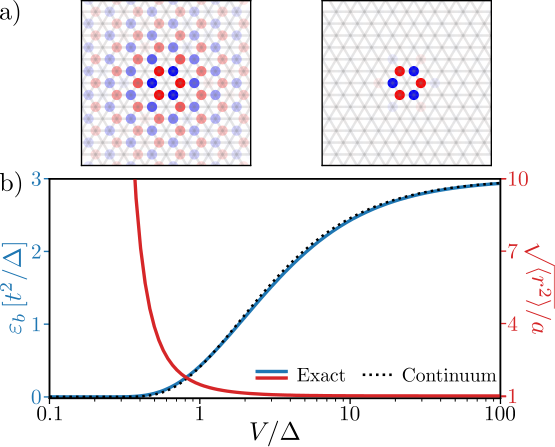
The two-particle bound state we found has zero total momentum, is symmetric under three-fold rotation, and changes sign under reflection that flips one of the primitive vectors , i.e. it has -wave pairing symmetry. The size of the bound state shrinks with increasing , as shown in the inset of Fig. 2 for and . At small , the pair wavefunction is highly extended over many lattice sites, while in the opposite limit , two nearest-neighbor fermions form the most tightly bound pair “resonating” within a single upper triangle (see Sup). Our solution of the two-particle problem suggests a crossover between BCS and BEC states at small particle density, tuned by .
The presence of a two-particle bound state is a striking feature of our mechanism, distinct from the Kohn-Luttinger mechanism Kohn and Luttinger 1965, which relies on the presence of a filled Fermi sea to mediate an effective attraction between electrons. Here on the contrary, pairing is already present for two doped fermions, and is induced by virtual excitation of the insulating state.
We now extend our analysis to finite, but small, doping concentrations above . In this regime, the physics of dilute doped fermions is governed by long-wavelength properties that transcend the details on the lattice scale. This motivates us to derive a low-energy theory by taking the continuum limit of the lattice Hamiltonian. This is achieved by rewriting the lattice Hamiltonian in terms of fermionic fields in momentum space and retaining only modes near the bottom of the -band. Importantly, the band dispersion , with , has two degenerate minima located at the points of the Brillouin zone. Therefore, low-energy degrees of freedom are described by two long-wavelength fermionic fields with , distinguished by the valley index . In the supplementary materials Sup, we find the following continuum Hamiltonian for :
| (5) |
where the effective mass and interaction strength are entirely determined from the lattice parameters:
| (6) |
The resulting quantum field theory describes a two-flavor fermion gas in the continuum with attractive contact interaction. The two flavors correspond to the valley degree of freedom associated with the underlying lattice, from which the field theory is derived. This theory is asymptotically exact in the low doping limit where -wave scattering between fermions of opposite valleys is the dominant interaction.
This attractive interaction leads to the formation valley-singlet two-particle bound states, which exactly correspond to the -wave pairs observed on the lattice (see Fig. 2). Indeed, the pair amplitude is odd under the reflection that interchanges the two valleys. To verify the validity of our continuum model, we calculate the two-particle binding energy in the field theory, and using the parameters and given by Eq. (Results) and (3), compare it with the exact solution of the lattice model. The expression for is
| (7) |
with an energy cutoff that we fix with the exact binding energy at Sup. The exponent in Eq. (Results), defined by the ratio of effective pairing interaction and the bandwidth, only depends on the ratio in the narrow band regime . Remarkably, a perfect agreement between continuum theory and lattice model is found at all values of (see Fig. 2). This proves the accuracy of our mapping from lattice model to continuum theory.
Let us summarize our achievements so far. We have transformed the strongly repulsive model (Eq. Results), into an effective Hamiltonian for doped particles featuring attractive interaction. When the single particle bandwidth is small, this transformation is exact and the two-particle pairing problem is solved exactly. The nature of the ground state at low density depends on the strength of this attraction, measured by the dimensionless coupling constant . If is small, the binding energy is small compared to the Fermi energy and the doped charge form a weakly attractive Fermi gas. On the other hand, a large will produce tightly bound pairs. One can tune between these two regimes by increasing the ratio , as shown Fig. 2a.
The attractive Fermi gas in two dimensions is known to be superconducting at low temperature and exhibits a BCS-BEC crossover as the ratio between pair binding and Fermi energies changes from small to large values Randeria et al. 1989; Bertaina and Giorgini 2011; Parish 2015. In the region of weakly bound pairs , the critical temperature is given by with Euler’s constant Miyake 1983; Petrov et al. 2003. In terms of the dimensionless coupling constant (Eq. (Results)), we obtain the explicit formula for :
| (8) |
where the Gorkov Melik-Barkhudarov corrections have been included to correctly describe the strong coupling nature of the superconducting state Gor’kov and Melik-Barkhudarov 1961; Chubukov et al. 2016. As an example, this formula safely applies at if , where we both have and Bertaina and Giorgini 2011, as confirmed thereafter by exact diagonalization.
On the other side of the crossover , the physics depends on the interaction between the bosonic pairs. When these bosons repel, the system exhibits a BKT transition toward a BEC at low temperature Fisher and Hohenberg 1988, while it collapses if bosons attract Ruprecht et al. 1995; Roberts et al. 2001. Between the extreme BCS and BEC limits, the critical temperature satisfies the very general bound Hazra et al. 2019, which limits the largest achievable .
The BCS-BEC crossover of the two-dimension Fermi gas can be achieved by tuning either carrier density or the interaction strength , which is controlled by in our model. We plot in Fig. 3 the critical temperature as a function of doping concentration and . At very low doping where , the system lies in the BEC regime and increases rapidly with . At some critical concentration, the system undergoes the BEC-BCS crossover and finally follows Eq. (8).
It is worth emphasizing that our exact BCS formula Eq. (8) applies provided that the dimensionless coupling constant is small, even when the bare repulsion far exceeds the bandwidth . This is because doped fermions at the conduction band bottom reside entirely on sublattice, and therefore avoid the direct nearest-neighbor repulsion . In the weak-coupling regime , the attraction between low-energy carriers is induced by virtual interband particle-hole pairs or excitons, and leads to exponentially small . Most importantly however, our expression of is nonperturbative in and remains exact at , where strong-coupling superconductivity and maximum are attained. For instance, at doping , reaches around , which is about of the quasiparticle bandwidth .
Materials and Methods
We support the emergence of superconductivity with evidence from ED on finite size lattices. While the original model Eq. (Results) exhibits positive Sup, we focus on the effective model Eq. (2) which allows to reach larger system sizes. First, the superfluid behavior of the system is probed by the charge stiffness Kohn 1964
| (9) |
at doping , with the number of doped fermions and the number of sites along the two basis vectors of the triangular lattice. measures the sensitivity of the ground state energy to twisted boundary conditions . A positive value of in the thermodynamic limit implies dissipationless charge transport and gives a direct signature of the Meissner effect Scalapino et al. 1993. In the range of parameters considered, our system clearly exhibits (with small finite-size effect) the flux periodicity of superconductors Loder et al. 2008 and shows positive (see Fig. 4a-b), which proves superconductivity in the ground state. The charge stiffness of a BCS superconductor with a parabolic dispersion relation is known exactly: Hazra et al. 2019. Our results for are correctly captured by this prediction, especially at low doping concentrations where fermions live close to the band minima.
To demonstrate the strong-coupling nature of the superconducting state, we consider the superconducting gap
| (10) |
Our continuum theory Eq. (5) predicts up to . This leads to a ratio of the gap and critical temperature Miyake 1983; Petrov et al. 2003; Gor’kov and Melik-Barkhudarov 1961, which is much larger than the universal value in BCS theory for weak-coupling superconductors Schrieffer 2018. This is because the phonon-induced retarded attraction in conventional metals is limited to electrons within a Debye energy from the Fermi surface, whereas in our theory the induced pairing interaction is instantaneous on the time scale of inverse bandwidth (), so that all carriers in the narrow band are subject to the pairing interaction. For sufficiently large or at very small doping concentrations, the system lies in the BEC regime and the gap to ratio can take arbitrarily large values.
Our numerical results for , shown in Fig. 4c, confirm the superconducting behaviors identified above with a robust gap increasing with up to . Near this point, our numerical results agree with the mean field prediction, and the gap reaches as large as . This allows the system to reach critical temperature of 0.1, as described above. For , the numerically extracted gaps lie above the continuum theory prediction due to finite size effects. Indeed in that regime, the finite lattice considered cannot fully accommodate the large-sized bound state that arise in the thermodynamic limit (see Fig. 2). This effective confinement increases the energy of the bound pairs, resulting in an overestimate of the superconducting gap. Despite this discrepancy, the simultaneous presence of a positive and a non-zero charge stiffness stands as a strong probe of superconductivity in our model for .
In addition to the BCS-BEC superconductivity at low density, our model shows very rich physics at higher doping concentrations, where lattice effects become important. By performing mean-field calculation on the model Eq. (2), we find -wave pairing for doping (see supplementary materials Sup). The corresponding critical temperatures, shown in Fig. 3, are calculated with the linearized gap equation
| (11) |
with and , where originates from three-body interactions. Here, denotes the total number of sites, and the chemical potential is fixed by , with the Fermi-Dirac distribution.
At low doping, the -wave superconducting state has a full pairing gap and its obtained from lattice model calculation agrees well with our previous result based on continuum theory. Interestingly, at higher doping concentration , the gap vanishes at 6 nodes on the Fermi surface along direction, where the -wave gap function vanishes. This change in gap structure is due to the change of Fermi surface topology across the van Hove singularity, where the two pockets around merge into a single Fermi surface enclosing the point (see Fig. 3).
The above conclusions are confirmed by our ED study, which shows clear evidence of nodal superconductivity at . We also find that the superconducting state is remarkably robust against longer range bare repulsion. These numerical results can respectively be found in the supplementary materials Sup.
Finally, our ED study reveals non-superconducting states in the ultrastrong coupling regime Sup. The detailed description of these competing phases is left for further study, the focus of this work being the fully-controlled theory of superconductivity emerging from repulsive interactions at .
Discussion
Our work opens a new route to unconventional superconductivity in atomic Fermi gas and electron systems. Encouragingly, optical lattice with honeycomb geometry and tunable band gap have already been realized Uehlinger et al. 2013; Fläschner et al. 2016. Many recent advances in dipolar or Rydberg atom systems with longer-range interactions Baier et al. 2018; Lu et al. 2012 have enabled the implementation of one-dimensional Hamiltonian Guardado-Sanchez et al. 2020, and hold great promise for the realization of our model in near future.
Our mechanism for strong-coupling superconductivity mediated by charge-transfer complex, or interband excitations, may also shed insight on graphene-based moiré superlattices, where the small bandwidth and high ratio (up to ) place important constrains on viable theories. It will be interesting to develop accurate low-energy models for these systems and analyze superconductivity in the narrow band limit as exemplified in our work. In this regard, we note that correlated hopping and direct repulsion also appear in effective Hamiltonian for narrow bands in twisted bilayer graphene Guinea and Walet 2018; Kang and Vafek 2019; Koshino et al. 2018. Our theory suggests that renormalization by virtual interband excitations is necessary to obtain strong-coupling superconductivity. Moreover, our simple model may be relevant to twisted double bilayer graphene Liu et al. 2020 and trilayer graphene-boron nitride heterostructures Chen et al. 2019, where signs of spin-polarized superconductivity has been reported Lee et al. 2019; Cornfeld et al. 2020. We leave to future work the extension of our theory to spinful systems and its application to various strongly-correlated materials.
Acknowledgments. We thank K. Slagle and A. Chubukov for valuable comments on the manuscripts. This work was supported by DOE Office of Basic Energy Sciences, Division of Materials Sciences and Engineering under Award DE-SC0018945. LF was supported in part by a Simons Investigator Award from the Simons Foundation.
Author contributions. Both authors contributed essentially to the formulation and theoretical analysis of the problem and to writing the manuscript. VC performed numerical calculations.
Statement on competing interests. All authors declare that they have no competing interests.
Data and materials availability. All data needed to evaluate the conclusions in the paper are present in the paper and/or the Supplementary Materials.
References
- Bardeen et al. (1957) J. Bardeen, L. N. Cooper, and J. R. Schrieffer, Theory of superconductivity, Physical review 108, 1175 (1957).
- Fröhlich (1950) H. Fröhlich, Theory of the superconducting state. i. the ground state at the absolute zero of temperature, Physical Review 79, 845 (1950).
- Bardeen and Pines (1955) J. Bardeen and D. Pines, Electron-phonon interaction in metals, Physical Review 99, 1140 (1955).
- Morel and Anderson (1962) P. Morel and P. Anderson, Calculation of the superconducting state parameters with retarded electron-phonon interaction, Physical Review 125, 1263 (1962).
- Bogoljubov et al. (1958) N. Bogoljubov, V. V. Tolmachov, and D. Širkov, A new method in the theory of superconductivity, Fortschritte der physik 6, 605 (1958).
- Lin et al. (2013) X. Lin, Z. Zhu, B. Fauqué, and K. Behnia, Fermi surface of the most dilute superconductor, Phys. Rev. X 3, 021002 (2013).
- Cao et al. (2018) Y. Cao, V. Fatemi, S. Fang, K. Watanabe, T. Taniguchi, E. Kaxiras, and P. Jarillo-Herrero, Unconventional superconductivity in magic-angle graphene superlattices, Nature 556, 43 (2018).
- Lu et al. (2019) X. Lu, P. Stepanov, W. Yang, M. Xie, M. A. Aamir, I. Das, C. Urgell, K. Watanabe, T. Taniguchi, G. Zhang, et al., Superconductors, orbital magnets and correlated states in magic-angle bilayer graphene, Nature 574, 653 (2019).
- Park et al. (2020) J. M. Park, Y. Cao, K. Watanabe, T. Taniguchi, and P. Jarillo-Herrero, Tunable phase boundaries and ultra-strong coupling superconductivity in mirror symmetric magic-angle trilayer graphene, arXiv preprint arXiv:2012.01434 (2020).
- Hao et al. (2020) Z. Hao, A. Zimmerman, P. Ledwith, E. Khalaf, D. H. Najafabadi, K. Watanabe, T. Taniguchi, A. Vishwanath, and P. Kim, Electric field tunable unconventional superconductivity in alternating twist magic-angle trilayer graphene, arXiv preprint arXiv:2012.02773 (2020).
- Norman (2011) M. R. Norman, The challenge of unconventional superconductivity, Science 332, 196 (2011).
- Phillips et al. (1998) P. Phillips, Y. Wan, I. Martin, S. Knysh, and D. Dalidovich, Superconductivity in a two-dimensional electron gas, Nature 395, 253 (1998).
- Ruhman and Lee (2016) J. Ruhman and P. A. Lee, Superconductivity at very low density: The case of strontium titanate, Physical Review B 94, 224515 (2016).
- Qin et al. (2020) M. Qin, C.-M. Chung, H. Shi, E. Vitali, C. Hubig, U. Schollwöck, S. R. White, S. Zhang, et al., Absence of superconductivity in the pure two-dimensional hubbard model, Physical Review X 10, 031016 (2020).
- Raghu et al. (2010) S. Raghu, S. Kivelson, and D. Scalapino, Superconductivity in the repulsive hubbard model: An asymptotically exact weak-coupling solution, Physical Review B 81, 224505 (2010).
- Maiti and Chubukov (2013) S. Maiti and A. V. Chubukov, Superconductivity from repulsive interaction, in AIP Conference Proceedings, Vol. 1550 (American Institute of Physics, 2013) pp. 3–73.
- Khaliullin and Chaloupka (2008) G. Khaliullin and J. Chaloupka, Origin of strong correlations and superconductivity in na x coo 2, Physical Review B 77, 104532 (2008).
- Nandkishore et al. (2014) R. Nandkishore, R. Thomale, and A. V. Chubukov, Superconductivity from weak repulsion in hexagonal lattice systems, Physical Review B 89, 144501 (2014).
- Slagle and Fu (2020) K. Slagle and L. Fu, Charge transfer excitations, pair density waves, and superconductivity in moiré materials, Phys. Rev. B 102, 235423 (2020).
- Schrieffer and Wolff (1966) J. R. Schrieffer and P. A. Wolff, Relation between the anderson and kondo hamiltonians, Physical Review 149, 491 (1966).
- MacDonald et al. (1988) A. H. MacDonald, S. Girvin, and D. t. Yoshioka, t/u expansion for the hubbard model, Physical Review B 37, 9753 (1988).
- (22) See supplementary materials at url.
- Kohn and Luttinger (1965) W. Kohn and J. M. Luttinger, New mechanism for superconductivity, Phys. Rev. Lett. 15, 524 (1965).
- Randeria et al. (1989) M. Randeria, J.-M. Duan, and L.-Y. Shieh, Bound states, cooper pairing, and bose condensation in two dimensions, Physical review letters 62, 981 (1989).
- Bertaina and Giorgini (2011) G. Bertaina and S. Giorgini, Bcs-bec crossover in a two-dimensional fermi gas, Physical review letters 106, 110403 (2011).
- Parish (2015) M. M. Parish, The bcs–bec crossover, in Quantum Gas Experiments: Exploring Many-Body States (World Scientific, 2015) pp. 179–197.
- Miyake (1983) K. Miyake, Fermi liquid theory of dilute submonolayer 3he on thin 4he ii film: dimer bound state and cooper pairs, Progress of theoretical physics 69, 1794 (1983).
- Petrov et al. (2003) D. Petrov, M. Baranov, and G. Shlyapnikov, Superfluid transition in quasi-two-dimensional fermi gases, Physical Review A 67, 031601 (2003).
- Gor’kov and Melik-Barkhudarov (1961) L. Gor’kov and T. Melik-Barkhudarov, Contribution to the theory of superfluidity in an imperfect fermi gas, Sov. Phys. JETP 13, 1018 (1961).
- Chubukov et al. (2016) A. V. Chubukov, I. Eremin, and D. V. Efremov, Superconductivity versus bound-state formation in a two-band superconductor with small fermi energy: Applications to fe pnictides/chalcogenides and doped srtio 3, Physical Review B 93, 174516 (2016).
- Fisher and Hohenberg (1988) D. S. Fisher and P. Hohenberg, Dilute bose gas in two dimensions, Physical Review B 37, 4936 (1988).
- Ruprecht et al. (1995) P. Ruprecht, M. Holland, K. Burnett, and M. Edwards, Time-dependent solution of the nonlinear schrödinger equation for bose-condensed trapped neutral atoms, Physical Review A 51, 4704 (1995).
- Roberts et al. (2001) J. L. Roberts, N. R. Claussen, S. L. Cornish, E. A. Donley, E. A. Cornell, and C. E. Wieman, Controlled collapse of a bose-einstein condensate, Physical Review Letters 86, 4211 (2001).
- Hazra et al. (2019) T. Hazra, N. Verma, and M. Randeria, Bounds on the superconducting transition temperature: Applications to twisted bilayer graphene and cold atoms, Physical Review X 9, 031049 (2019).
- Kohn (1964) W. Kohn, Theory of the insulating state, Phys. Rev. 133, A171 (1964).
- Scalapino et al. (1993) D. J. Scalapino, S. R. White, and S. Zhang, Insulator, metal, or superconductor: The criteria, Physical Review B 47, 7995 (1993).
- Loder et al. (2008) F. Loder, A. P. Kampf, and T. Kopp, Crossover from to current oscillations in rings of -wave superconductors, Phys. Rev. B 78, 174526 (2008).
- Schrieffer (2018) J. Schrieffer, Theory Of Superconductivity (CRC Press, 2018).
- Uehlinger et al. (2013) T. Uehlinger, G. Jotzu, M. Messer, D. Greif, W. Hofstetter, U. Bissbort, and T. Esslinger, Artificial graphene with tunable interactions, Physical review letters 111, 185307 (2013).
- Fläschner et al. (2016) N. Fläschner, B. Rem, M. Tarnowski, D. Vogel, D.-S. Lühmann, K. Sengstock, and C. Weitenberg, Experimental reconstruction of the berry curvature in a floquet bloch band, Science 352, 1091 (2016).
- Baier et al. (2018) S. Baier, D. Petter, J. Becher, A. Patscheider, G. Natale, L. Chomaz, M. Mark, and F. Ferlaino, Realization of a strongly interacting fermi gas of dipolar atoms, Physical review letters 121, 093602 (2018).
- Lu et al. (2012) M. Lu, N. Q. Burdick, and B. L. Lev, Quantum degenerate dipolar fermi gas, Physical Review Letters 108, 215301 (2012).
- Guardado-Sanchez et al. (2020) E. Guardado-Sanchez, B. Spar, P. Schauss, R. Belyansky, J. T. Young, P. Bienias, A. V. Gorshkov, T. Iadecola, and W. S. Bakr, Quench dynamics of a fermi gas with strong long-range interactions, arXiv preprint arXiv:2010.05871 (2020).
- Guinea and Walet (2018) F. Guinea and N. R. Walet, Electrostatic effects, band distortions, and superconductivity in twisted graphene bilayers, Proceedings of the National Academy of Sciences 115, 13174 (2018).
- Kang and Vafek (2019) J. Kang and O. Vafek, Strong coupling phases of partially filled twisted bilayer graphene narrow bands, Phys. Rev. Lett. 122, 246401 (2019).
- Koshino et al. (2018) M. Koshino, N. F. Q. Yuan, T. Koretsune, M. Ochi, K. Kuroki, and L. Fu, Maximally localized wannier orbitals and the extended hubbard model for twisted bilayer graphene, Phys. Rev. X 8, 031087 (2018).
- Liu et al. (2020) X. Liu, Z. Hao, E. Khalaf, J. Y. Lee, Y. Ronen, H. Yoo, D. H. Najafabadi, K. Watanabe, T. Taniguchi, A. Vishwanath, et al., Tunable spin-polarized correlated states in twisted double bilayer graphene, Nature 583, 221 (2020).
- Chen et al. (2019) G. Chen, A. L. Sharpe, P. Gallagher, I. T. Rosen, E. J. Fox, L. Jiang, B. Lyu, H. Li, K. Watanabe, T. Taniguchi, et al., Signatures of tunable superconductivity in a trilayer graphene moiré superlattice, Nature 572, 215 (2019).
- Lee et al. (2019) J. Y. Lee, E. Khalaf, S. Liu, X. Liu, Z. Hao, P. Kim, and A. Vishwanath, Theory of correlated insulating behaviour and spin-triplet superconductivity in twisted double bilayer graphene, Nature communications 10, 1 (2019).
- Cornfeld et al. (2020) E. Cornfeld, M. S. Rudner, and E. Berg, Spin-polarized superconductivity: order parameter topology, current dissipation, and multiple-period josephson effect, arXiv e-prints , arXiv (2020).
- Vidal et al. (2000) J. Vidal, B. Douçot, R. Mosseri, and P. Butaud, Interaction induced delocalization for two particles in a periodic potential, Physical review letters 85, 3906 (2000).
- Levinsen and Parish (2015) J. Levinsen and M. M. Parish, Strongly interacting two-dimensional fermi gases, in Annual review of cold atoms and molecules (World Scientific, 2015) pp. 1–75.
Supplemental Materials: New mechanism and exact theory of superconductivity from strong repulsive interaction
Valentin Crépel, Liang Fu
Massachusetts Institute of Technology, 77 Massachusetts Avenue, Cambridge, MA, USA
S1 Schrieffer-Wolff Transformation
In this appendix, we derive effective model Eq. 2 with a Schrieffer-Wolff transformation. This effective Hamiltonian is exact up to corrections of order , irrespective of the ratio .
S1.1 Canonical Transformation
Single particle tunneling on the honeycomb lattice couples the -band to trimers, polarons and dipoles. The Schrieffer-Wolff transformation uses a canonical transformation , with Hermitian, to treat these couplings as an effective Hamiltonian that leaves the -band invariant up to second order correction in . This is achieved if satisfies
| (S1) |
as can be seen with the Baker-Campbell-Haussdorf formula. Under the assumption Eq. S1, we get
| (S2) |
To find , we follow Ref. MacDonald et al. 1988 and split the tunneling Hamiltonian into a collection of operators
| (S3) |
where gathers all tunneling operations that change the number of occupied sites by and the number of occupied nearest neighbor pairs by , i.e. it changes the energy of ’s eigenstates by . The bounds for and are determined by the lattice geometry. With these definition, we can check that
| (S4) |
satisfies Eq. S1. Consider an eigenstate of with energy . By definition is also an eigenstate of with energy . As a consequence, we have
| (S5) |
Finally, the relation ensures the hermiticity of . Plugging Eq. S4 into Eq. S2, we find the generic expression
| (S6) |
To evaluate the correcting terms of this last equation, we have noticed that all terms in are smaller than in magnitude.
S1.2 Low energy projection
To describe the low-energy properties of our model, we project the obtained Hamiltonian onto the -band which is well separated from other excitations by the charge transfer gap . This projection restricts the sum in Eq. S6 to cases where and . Furthermore, the first operator acting on the states of the -band should move an electron from an to a site, i.e. the rightmost must have . This gives
| (S7) |
The three terms of the sum gather all second order processes that respectively involve the virtual occupation of a trimer, a polaron and a dipole excitation (shown in Fig. 1). As expected from second order perturbation theory, these processes occur with rates
| (S8) |
that are inversely proportional to their energy difference with the -band.
S1.3 Simplification
To further simplify , we isolate the contributions of Eq. S7 depending on the number of occupied neighbor of each -site. In the following, we focus on a -site at position and denote its three neighbors as , and .
No neighboring fermions:
If the -site is surrounded by three empty sites, it can couples to three different dipole excitations in which the fermion at is moved on a neighboring site. This provides an energy shift
| (S9) |
One neighboring fermion:
If the -site has a neighboring fermion at position , it can couples to two polarons by hopping to either or . If the second tunneling process in Eq. S7 moves it back to , the process leads to an energy shift. On the contrary, if the fermion at replace the original one at , the process can be viewed as an effective tunneling of the -fermion on a neighboring -site. Together, they give
| (S10) |
Note that the tunneling terms come with a positive sign due to the anticommutation relation between fermions. Circular permutation of the indices gives all other possible terms involving a polaron.
Two neighboring fermions:
Finally, if and both host a fermion, the system can only couple to a trimer excitation by moving the electron to . The second tunneling process can either put this fermion back to , leading to en energy reduction, or put the ones at or at , giving a density-assisted tunneling term:
| (S11) |
Again, circular permutation of the indices gives all other possible terms involving a trimer.
Gathering the contributions of a-b-c, we obtain the effective Hamiltonian Eq. 2 where the coefficients originates from the processes outlined in Fig. 1. The single particle fermion tunneling only appears in Eq. S10 and therefore reads . The correlated tunneling appears in Eqs. S11 and S10 with opposite signs: . Two-body and three-body interaction coefficients come from the three cases a-b-c. Carefully counting all terms, we find and . These expression are given in Eq. 3, and plotted against in Fig. S1. For comparison (see text), we also show the results from the projection of the bare repulsion into the -band, valid when .
S2 Solution of the two body problem
In this appendix, we solve the effective lattice model Eq. 2 for two fermions. To understand the competing roles of two-body interaction and correlated hopping, we first look at the quartic part of the Hamiltonian (Sec. S2.1). Then, we decouple the center of mass and relative motions of the two fermions (Sec. S2.2) and explain in more detail how the results presented in the main text were obtained (Sec. S2.3).
S2.1 ’Resonating’ triangle
We start with the quadratic terms of our model
| (S12) |
All states where the two electrons are not neighbors are zero energy eigenstates of this operator. The others have two doped charge on the same upper triangle, and can be divided into irreducible representations of . More precisely, there is a state in the identity representation and an -doublet
| (S13) |
with the insulating state at unit filling, which also corresponds to the vacuum for the operators. These three eigenstates of have energy
| (S14) |
Because , the lowest energy manifold is made of all states and has negative energy, corresponding to bound states. As mentioned in the main text, this binding energy solely comes from correlated hopping when , for which . These dimers have the -wave symmetry described in the main text (see Fig. 2), and can be seen as dimers ’resonating’ within an upper triangle as shown in Fig. S2.
This solution unveils the crucial role of correlated tunneling for pairing and gives an intuitive real-space picture for the bound pairs. It also allows to better understand the low energy continuum model Eq. 5. First, the coupling constant is directly proportional to the energy . Moreover, it also gives a physical intuition for the -wave scattering between the two valleys. To see this, let’s reintroduce the tunneling in the lowest energy subspace to lift the degeneracy of the low energy manifold (this perturbative treatment of is justified in the limit ). The dispersion relation of the bound pairs has its minimum at the point. The lowest energy state is
| (S15) |
with . The amplitude of the paired state is maximal in magnitude near the and points, as shown in Fig. S2. This confirms our intuition that the dominant scattering channel couples electrons with different isospin in -wave to form valley singlets. While this argument gives an intuitive understanding of the dominant pairing interaction in our system, it can only be formally applied in the limit where where the tunneling can be treated as a perturbation to .
S2.2 Center of mass and relative motion
To solve the two-particle problem exactly, we now decouple the center of mass and relative motion of the two fermions. Taking all terms of Eq. 2 simultaneously into account, we obtain the results presented in Fig. 2, which also agree with the previous perturbative treatment of the previous section in the limit .
The Hilbert space with two fermions is spanned by the states
| (S16) |
Taking advantage of the translation invariance of the problem, we can introduce the center of mass momentum and reorganize the Hilbert space with the Bloch-waves Vidal et al. 2000
| (S17) |
Because , the state with opposite relative positions describe the same physical state . To avoid double counting the states, we restrict our attentions to states with . The action of the Hamiltonian in this new basis can be directly computed
| (S18) | ||||
As expected from translation invariance, the state only couple to states with the same center of mass momentum . The tunneling on the lattice acts as an effective hopping term for the relative position . The local interaction and correlated tunneling terms only changes this tight-binding Hamiltonian close to the origin for or with . This tight binding Hamiltonian can be solved numerically for each center of mass momentum . Its ground state always is at the point, and reads . Its energy yields the binding energy and bound state size
| (S19) |
in Fig. 2. Of course, accurate results can only be obtained when the system size exceeds the spread of the two-fermion bound state. In particular for , the bound state size sharply increases and a more careful extraction of the energy is required.
S2.3 Finite size scaling
We therefore focus on the regime , and extract the two-body problem as a function of the inverse number of site in the system as shown in Fig. S3. Linear interapolation of these curves at gives the values of the binding energy in the thermodynamic limit. The interpolated values are reported in Fig. 2. It is worth pointing out that we infer positive pair binding energy in the entire range , in agreement with the continuum model.
S3 Continuum model
S3.1 Derivation
In this appendix, we derive the continuum model Eq. 5 in the limit of small doping concentration. Focusing on the physics near the and pockets, and discarding all high energy fermionic degrees of freedom amounts to write the Fourier transform of the -operators as
| (S20) |
with the number of honeycomb unit cells. Total momentum conservation restricts the interaction terms to valley-preserving ones. They can be further decomposed as intra-valley interactions
| (S21) |
and inter-valley interactions
| (S22) |
which both depend on the momentum space representation of the quartic terms of Eq. 2:
| (S23) |
Due to the small momenta considered in our continuum theory, we can Taylor expand the previous expression with the help of the relations
| (S24) |
which hold true up to corrections. This leading order approximation and the fermion anti-commutation relations show that intra-valley interactions are negligible compared to inter-valley ones
| (S25) |
with . Fourier transforming back to real-space and accounting for the Brillouin zone area, we obtain the effective interaction announced in Eq. 5:
| (S26) |
S3.2 Binding Energy
As a consistency check of our continuum model Eq. 5, we can determine the binding energy and compare it with the exact solution found in App. S2. Using a -matrix approach, the binding energy of the continuum theory is solution of the implicit equation Levinsen and Parish 2015
| (S27) |
Going to polar coordinates and introducing the momentum UV cutoff , we find
| (S28) |
which can be integrated to obtain
| (S29) |
S4 Longer range interactions
In this appendix, we show evidence that longer range interactions neither destroy the effective pairing between doped charges nor the superconducting phase described in the main text. We include next-nearest neighbor interactions in order to describe the tail of the fermion-fermion interaction.
The range of next-nearest interaction strength relevant for our work is . In that regime, the Schrieffer-Wolff transformation of App. S1 almost identically applies, up to two corrections. To first order, introduces a direct interaction between electron in the -band. To second order in , it also changes the denominators of Eq. 3, which are determined by the new dipole, polaron and trimer energies:
| (S31) |
For weak perturbations , the second corrections can be safely discarded, and we obtain the same effective model as Eq. 2 with a two-body interaction strength
| (S32) |
At small doping, we can go to the continuum and the system is described by Eq. 5 with a modified coupling constant (compare with Eq. Results). When the additional interaction term is smaller than the largest pair binding energy of the original problem, i.e. , we find a that is negative when , where
| (S33) |
In other words, at small , longer range interactions in the range only shifts the range of where superconductivity is observed. For larger , the bound pairs breaks to avoid large next-nearest neighbor repulsion and the binding energy is always negative.
Even in that regime, the superconducting phase can reappear at larger doping concentrations. Indeed, if they are closely packed, the fermions of a pair do not decrease their energy by splitting apart because this send them closer to all the other surrounding fermions in the system. We evidence the stability of the superconducting phase against at large doping with ED with 4 and 6 particles in a lattice, thus at doping and , with . The charge stiffness extracted as a function of is shown in Fig. S4. Despite a slight decrease, the stiffness remains positive up to . This gives support for the stability of the superconducting phase against longer range interactions at doping .
Finally, the regime has been extensively described in the in Ref. Slagle and Fu 2020. In that case, the trimer energy can be resonant with the -band. The presence of these preformed pairs in the Fermi sea of doped charges leads to superconductivity and pair-density waves. While the origin of pairs is different in that regime, strong interactions can still lead to superconductivity.
S5 Pairing and superconductivity in the full-fledged model

We present ED results on the original model Eq. Results in Fig. S5, which give further evidence for the presence of two-body bound pairs at finite doping above the insulating state, and for the emergence of superconductivity in our model. The former is probed by the pair binding energy that we find, as in the main text, positive in the limit for the entire range of considered. For , we also observe a region with positive pair binding energy for sufficiently large .
To investigate the superconducting correlations in the ground state of the doped insulator, we calculate the -wave pair correlation function
| (S34) |
with . A superconducting state with -wave symmetry is expected to exhibit a power-law decay of with distance, and hence to have sizable correlations at large distances. For the largest accessible finite size clusters , the maximum distance is achieved for . We denote the pair correlation function at this distance as . In Fig. S5, we show as a function of the parameters for several . We observe large correlations in the perturbative limit when , where we indeed expect a strong superconducting order (see, for instance, Fig. 3). This direct manifestation of superconductivity gives strong evidence for the reliability of the predictions made from the effective model Eq. 2 and its mean-field solution detailed below in App. S6.
S6 Mean-field treatment
S6.1 Dilute limit
We now carry out a self-consistent mean field treatment of the low-energy model Eq. 2 in the dilute limit, where three-body interaction terms are negligible. Going to Fourier space, the Hamiltonian becomes
| (S35) |
with defined in Eq. S23. Then we perform the mean-field substitution . This replacement leads to the following quadratic mean-field Hamiltonian
| (S36) |
where we have introduced a chemical potential and the short notation . We have also used the relation . The quadratic Hamiltonian is diagonalized as
| (S37) |
through the Bogoliubov transformation
| (S38) | ||||
The ground state of the system is annihilated by all quasi-particle operators and takes the form . The order parameter may now be computed self-consistently through the calculation of the correlators . This gives the so-called gap equation
| (S39) |
Using the explicit form of , this gap equation can be rewritten as
| (S40) |
with
| (S41) |
Similarly, the mean particle number fixes the chemical potential through the relation
| (S42) |
We solve the self-consistent gap equation numerically for infinitesimal doping and decompose the order parameter into partial and -wave. The results are shown in Fig. S6. We observe that the self-consistent always has a solution, with a substantial gap for . This provides another test of the continuum results of Fig. 3, where the critical temperature drastically rises near . Furthermore, our mean-field solution exhibits a strong -wave symmetry, which corroborates our exact two-fermion calculation (Fig. 2).
S6.2 Critical temperature and and three-body interactions
Including finite temperature effects to the previous analysis provides a way to determine the critical temperature at which the pair are all broken by thermal fluctuation and Schrieffer 2018. This definition agrees with the superconducting temperature in the BCS limit of our model. Note that it does not capture the physics of the BKT transition, explaining why we obtain in Fig. 3. Focusing on an order parameter with pure -wave symmetry, the gap and number equations become
| (S43a) | ||||
| (S43b) | ||||
We solve this implicit definition of numerically. The results, presented in the inset of Fig. S6 for , show a sharp increase of near . Excellent agreement is found with the continuum results of Fig. 3 in the small doping limit. For , the non-parabolicity of the dispersion relation leads to corrections to Eq. 8.
The three-body interaction terms of Eq. 2 can be partially reincorporated in Eq. S43 near via the substitution
where we have replace one quadratic operator by its expectation in the normal state and with the Fermi-Dirac distribution. This simply renormalizes the effective interaction and correlated hopping strength
| (S44) |
which leads to a similar replacement of by
| (S45) |
in Eq. S43, as declared in the main text. The results shown in Fig. 3 are obtained with this substitution.
For fillings , we must rely on Eq. S43, which correctly describes the merging of the pockets, while the two-flavor continuum model Eq. 5 assume them well-separated. At these doping concentrations, our calculations show that a superconducting state only appears for , in sharp contrast with the dilute regime where superconductivity extends to (see Fig. 4). Another stark difference with the dilute limit is the presence of nodes of the superconducting gap located at the Fermi surface, which now encloses the point.
S7 ED evidence for nodal superconductor
We present more evidence of this nodal superconductor from ED of the effective model for . We focus on lattices of size and with 8 particles and more, and extract the charge stiffness and the superconducting gap as in the main text. Our results are presented in Fig. S7. There, we observe that the system is not superconducting for , in agreement with the mean-field calculations of App. S6. The transition to occurs around , consistent with the mean-field value up to finite-size jitters. These observations comfort the presence of a superconducting phase at doping and moderate .
In the entire superconducting phase evidenced above, the superconducting gap is almost zero and decrease in magnitude with larger system size. This hints towards nodes of the superconducting gap at the Fermi energy, as expected from the Fermi surface topology and -wave symmetry of the order parameter (see text).
S8 Bosonic effective interactions and phase separation
In this appendix, we present our numerical results obtained outside of the superconducting region that we focus on in the main text. We have evaluated the charges stiffness of the ground state in a wide region of doping concentration and ratio . Our results are presented in Fig. S8 for lattices with and , which mitigate finite size effects. A white dashed line indicates where , and serves as an indicator to distinguish between the BCS and BEC limits predicted by the continuum model Eq. 5. As shown in the main text, the stiffness in the BCS region () slowly increases but remains close to , especially at small doping concentrations. In the BEC limit, we observe two different behaviors depending on the value of . First, the results at cannot reliably describe the thermodynamic behavior of the system as they were obtain for less than four particles. In that case, the small BEC is either a two-body or four-body bound state with a large effective mass. For larger doping, the lattice effects observed in the main text rule the physics and the charge stiffness drops down with increasing . We observe that this diminution comes with a reduction of the may-body spectrum gap, until the ground state becomes highly degenerate for the .
To understand these features, we investigate the scattering properties of the local bosons in the limit. To distinguish between attractive and repulsive interactions of pairs, we evaluate the second binding energy , which plays the same role as for the tightly bound pairs. The results presented to the right of Fig. S8, show a positive for . This signals attractive interaction, which leads to the collapse of the quasi-BEC and to phase-separation. The collapse of the BEC in favor of phase separation explains the large degeneracy observed for . The BEC collapse at large doping concentrations for is also evidenced by a decay of the superconducting gap for , as shown in Fig. S9. Note that the points in the range reproduce those of Fig. 4 in the main text.