Signatures of Chaos in Non-integrable Models of Quantum Field Theory
Abstract
We study signatures of quantum chaos in (1+1)D Quantum Field Theory (QFT) models. Our analysis is based on the method of Hamiltonian truncation, a numerical approach for the construction of low-energy spectra and eigenstates of QFTs that can be considered as perturbations of exactly solvable models. We focus on the double sine-Gordon, also studying the massive sine-Gordon and model, all of which are non-integrable and can be studied by this method with sufficiently high precision from small to intermediate perturbation strength. We analyse the statistics of level spacings and of eigenvector components, which are expected to follow Random Matrix Theory predictions. While level spacing statistics are close to the Gaussian Orthogonal Ensemble as expected, on the contrary, the eigenvector components follow a distribution markedly different from the expected Gaussian. Unlike in the typical quantum chaos scenario, the transition of level spacing statistics to chaotic behaviour takes place already in the perturbative regime. Moreover, the distribution of eigenvector components does not appear to change or approach Gaussian behaviour, even for relatively large perturbations. Our results suggest that these features are independent of the choice of model and basis.
Introduction.— The physics of non-integrable quantum systems has been successfully described by quantum chaos theory, which states that their spectral statistics are given by Random Matrix Theory (RMT) i.e. exhibit the same behaviour as matrices whose elements are randomly chosen from a Gaussian distribution. These conjectures Casati et al. 1980; Bohigas et al. 1984; Berry 1977 have been verified for a broad class of single-particle models, where they have been explained in terms of semi-classical periodic orbit theory Bogomolny 1988; Müller et al. 2004. More recently research focus has shifted to many-body systems Santos and Rigol 2010a; Santos and Rigol 2010b; Rigol and Santos 2010; D’Alessio et al. 2016; Alba 2015; Beugeling et al. 2015a; Beugeling et al. 2018; Beugeling et al. 2015b; Haque et al. 2020; Foini and Kurchan 2019; Chan et al. 2018, where RMT predictions have been verified numerically and in certain cases even analytically Kos et al. 2018; Bertini et al. 2018. Chaoticity tests in quantum many-body models are, however, almost exclusively limited to discrete (lattice) models, leaving continuous models unexplored. Among them, relativistic Quantum Field Theories (QFTs) and their dynamics lie at the cornerstone of important open questions of theoretical physics, like the black hole information paradox Hayden and Preskill 2007, making the study of ergodicity and chaos in QFT a topic of fundamental interest.
Significant progress in this direction has been made based on new theoretical concepts and indicators Sekino and Susskind 2008; Shenker and Stanford 2014; Maldacena et al. 2016. Nevertheless, the emergence of quantum chaos in QFT remains poorly understood in terms of the more traditional measures of level spacing and eigenvector statistics Haake 2010. Studying level spacing statistics is the best way of detecting level repulsion, the characteristic property of random matrix spectra. On the other hand, a Gaussian distribution of eigenvector components is an important indication of validity of the Eigenstate Thermalisation Hypothesis (ETH) Deutsch 1991; Srednicki 1999, which explains how thermalisation emerges from the dynamics of non-integrable quantum systems Hortikar and Srednicki 1998.
The main obstacle in performing chaoticity tests in QFT is that, unlike for lattice models of condensed matter physics, QFT models are continuous and thus live in an infinite dimensional Hilbert space. Therefore, exact computation of energy spectra is not an option for non-integrable models, and we inevitably resort to approximate numerical methods. The challenge is then to achieve sufficiently high accuracy in a sufficiently large part of the spectrum, so that a statistical analysis is possible and reliable. An ideal method for this task is the “Truncated Conformal Space Approach” (TCSA) Yurov and Zamolodchikov 1990; Yurov and Zamolodchikov 1991; Feverati et al. 1998, more generally the Hamiltonian truncation method Hogervorst et al. 2015; James et al. 2018. The TCSA is based on the algebraic toolkit of Conformal Field Theory (CFT) and insights from Renormalisation Group theory, which can capture efficiently non-perturbative effects in the low-energy spectrum, and is especially suitable for (1+1)D models. A pioneering study of quantum chaos indicators using this method was presented in Brandino et al. 2010 for the tricritical and tetracritical Ising field theories, demonstrating that their level spacing statistics agree with the theoretical expectations in both the integrable and non-integrable case, and observing their crossover for varying parameters.
In this Letter we study two independent and equally important signatures of quantum chaos, the distribution of level spacings as quantified by the consecutive level spacing ratios Oganesyan and Huse 2007; Atas et al. 2013 and the distribution of eigenvector components. We study a class of (1+1)D models: the sine-Gordon model (SG), which is integrable, and the double sine-Gordon (DSG), massive sine-Gordon (MSG) a.k.a. Schwinger–Thirring, and model, which are all non-integrable. We verify that level spacings follow the expected Poisson distribution for SG and GOE distribution for DSG, MSG and model to a very good approximation. GOE behaviour is actually observed already in the weakly perturbed CFT regime, in contrast to what typically happens in single-particle models. Surprisingly, we find that, even when the level spacing distribution is close to GOE, the eigenvector component distribution is markedly different from the Gaussian found in RMT Brody et al. 1981 (Fig. 1). On the contrary, it exhibits at best exponential scaling followed by an algebraically decaying tail, which contradicts the RMT prediction. This last feature is robust and independent of the model and parameter values. We validate our observations by pushing the limits of TCSA’s potential to achieve high accuracy and devising a reliable measure of truncation error, which is crucial for distinguishing physical behaviour from numerical artefacts.
Models, Method & Observables.— We consider the following models: the SG with Hamiltonian , the DSG , the MSG , and the model , where
| (1) | |||
The SG is a prototypical integrable QFT possessing topological excitations Zamolodchikov 1995; Feverati et al. 1998; Feverati et al. 1999; Fehér and Takács 2011 and is equivalent to the massive Thirring model Coleman 1975; Mandelstam 1975. It has applications in condensed matter and atomic physics Giamarchi 2004 and has been simulated experimentally Schweigler et al. 2017; Zache et al. 2020. The DSG is non-integrable and also topologically non-trivial Delfino and Mussardo 1998; Bajnok et al. 2001; Mussardo et al. 2004; Takács and Wágner 2006. Lastly, the MSG is equivalent to the Schwinger–Thirring model, reducing to (1+1)D QED at Coleman et al. 1975; Coleman 1976.
All the above models can be seen as perturbations of the free boson CFT by relevant operators and as such they can be studied using TCSA. This method yields numerical approximations of the low-energy spectrum of based on the simple idea of computing the matrix elements of in an energy-truncated basis of and diagonalising the resulting finite matrix approximation of . If does not couple significantly the low- with the high-energy spectrum of , which is true for relevant perturbations, then the numerical spectrum is expected to converge to the exact upon increasing the truncation cutoff . TCSA has been successfully applied to the SG Feverati et al. 1998; Feverati et al. 1999; Fehér and Takács 2011; Kukuljan et al. 2018; Kukuljan et al. 2020, DSG Bajnok et al. 2001; Takács and Wágner 2006 and recently also the Schwinger model, a special limit of MSG Kukuljan 2021, while a similar Hamiltonian truncation method has been used for the model Hogervorst et al. 2015; Rychkov and Vitale 2015; Rychkov and Vitale 2016; Bajnok and Lajer 2016; Elias-Miró et al. 2017.
Using TCSA we compute a low-energy part of the spectra and eigenvectors of the above models for various parameter values and analyse their statistics. More specifically, we compute the distributions of level spacings , of consecutive level ratios and defined as Oganesyan and Huse 2007
| (2) |
and of eigenvector components in the TCSA basis. Since all models are time-reversal symmetric, the corresponding RMT ensemble is the GOE where the -distribution is and that of is the restriction of the latter to the interval , with mean value Atas et al. 2013. Conversely, in integrable models level spacings follow the Poisson distribution Berry and Tabor 1977 with . Compared to other tests of level spacing statistics, has the advantage of being independent of the local level density, therefore no ‘unfolding’ Haake 2010 is necessary. For the eigenvector component distribution, the RMT prediction is Gaussian, resulting in the Porter–Thomas distribution for their absolute values Brody et al. 1981, while for integrable models it is expected to be algebraic Samajdar and Jain 2018.
To minimise numerical errors we use truncated bases much larger than in previous studies ( states at the highest cutoff). Moreover, to ensure our results are sufficiently accurate, we verify convergence using rather strict truncation error estimates, based on measures of their correlations at successive cutoffs (see figure captions and Supp. Mat. SM).


Level spacing statistics.— We start by analysing the statistics of values. Fig. 1.a shows the distribution for DSG at two different choices of parameter values, one integrable (SG) and one non-integrable . The parameters have been chosen so that the energy gap between the ground and first excited state is of the same order as the inverse system size (more precisely, where and is the SG breather mass SM). These values are within the perturbative regime where convergence is optimal. We observe that the two distributions agree quite well with the Poisson and GOE distributions, respectively. The change of statistics can be demonstrated by the mean value for varying at fixed (Fig. 1.a, inset). Starting from the Poisson value for , increases towards the GOE value, fluctuating close and below it. The complete dependence of on both and is shown in Fig. 2 in the form of a “phase diagram”. The is close to Poisson along the SG lines ( and ), whereas it approaches in the areas away from these lines.
By independently varying the perturbation strength parameters at fixed (Fig. 3) we find that is close to even in the immediate vicinity of the unperturbed CFT model, i.e. for , as long as the ratio is kept fixed at . This is somewhat surprising given that chaoticity typically emerges far from integrable points and outside the perturbative regime. Chaotic values can indeed be verified from first-order perturbation theory results (Fig. 3.a) SM. The fluctuations of can be partially attributed to the relatively small energy window (2000 levels), as random matrices of the same size display similar fluctuations. Nevertheless, we notice that is predominantly below , meaning that this is still a transitional, not completely chaotic behaviour.
The differences between at different cutoffs (Fig. 2) are negligible, with the best convergence achieved for small . However, even if converges at some cutoff to , this does not necessarily mean that this is the correct physical value, since a non-convergent spectrum is also likely to be RMT-like. For this reason, we check the convergence using an error estimate based on the averaged absolute differences of values between successive cutoffs and verifying that the error decreases with increasing cutoff SM. We empirically find that increasing or results in larger truncation errors, making the numerical data less reliable. Moreover, in TCSA convergence is achieved in the lowest part of the computed spectra, with the truncation effects increasing at higher levels. For the parameters of Fig. 1, a sufficiently good level of convergence of values is achieved for the lowest levels at (in units ).
Eigenvector statistics.— Let us focus on the statistics of eigenvector components in DSG. Fig. 1.b shows the distribution of their absolute values in log scale for the same choice of parameters as in Fig. 1.a, one exhibiting Poisson and the other GOE level spacing statistics. Despite the clear difference in the latter, the eigenvector distributions are practically the same in both cases and different from the Gaussian prediction of RMT. In the bulk of the distribution the scaling is at best exponential while the tails decay slower, like an algebraic function. This is in strong contrast with theoretical expectations for chaotic models Brody et al. 1981. To eliminate truncation effects, we have again restricted the analysis to the convergent low-energy part of the matrix .
To gain a deeper insight into this observation, we look more closely into the structure of the matrix . Fig. 4.a–e shows for DSG at increasing perturbation strength . We observe that for small , is characterised by an approximately block-diagonal form, which is easily explained by perturbation theory given that the CFT spectrum is organised in degenerate energy shells SM. For increasing this block structure fades away and becomes more uniform, even though a pattern of fine structure remains always visible.
Based on these observations, we analyse how the DSG eigenvector distribution depends on , whether it approaches the RMT prediction when moving from weak to strong perturbation, and how it changes from one block to another. The distributions inside a single block exhibit clearly exponential scaling in the bulk, still with slower decaying tails (Fig. 4.g). The slope of this exponential changes from block to block. The distribution in Fig. 1, which corresponds to a large window including many blocks, is actually a superposition of many exponential distributions. There is no significant change when increases from 0 to , the maximum value for which we achieved convergence (Fig. 4.h). In fact, the distribution remains unchanged even for larger , where truncation effects are non-negligible. At the same time, for any and well convergent at least for (Fig. 4.f).
Comparing the eigenvector statistics of different models in windows with , we find that they generally vary from model to model but are always different from Gaussian and at best exponential (Fig. 5.b). The model, in particular, deserves special attention. In this case, using the CFT as the unperturbed model to construct the truncation basis is inconvenient, so the massive Klein-Gordon (KG) model is used instead Hogervorst et al. 2015. In contrast to the CFT basis, in KG there is no degenerate shell structure. Nevertheless, the eigenvector distribution is once again very different from Gaussian and characterised by slowly decaying tails as in DSG. Lastly, comparing the single-block eigenvector distributions in SG at different (Fig. 5.a), we find that they are similar to those of DSG. These results clearly show that the discrepancy between the eigenvector distributions and RMT prediction, in particular the presence of slowly decaying tails, is robust under variations of the parameters, energy window, model and truncation basis.
Discussion.— We have shown that, while the level spacing statistics of the above studied non-integrable QFTs agree with RMT, their eigenvector component statistics are markedly different from RMT predictions. Both of the above features emerge already in the weakly perturbed CFT regime and persist unchanged beyond that, which suggests that they may be valid for any perturbation strength. Indeed, there is no indication that the scaling of the distributions changes with the perturbation, even when the CFT shell structure disappears. Moreover, the qualitative characteristics of the eigenvector distributions for different models are similar, irrespectively of integrability and even for quite different choices of truncation basis. The latter observation particularly rules out an explanation based on exceptional features of the CFT basis. An interesting open question is how the observed discrepancy affects the validity of ETH in (1+1)D QFT. Testing ETH using Hamiltonian truncation methods is, however, a more challenging problem, as it is supposed to hold in the thermodynamic limit where the perturbation strength is large and convergence of the spectra worsens. We hope to investigate this question in the future.
The data presented in this work may be accessed at Srdinšek et al. 2020.
Acknowledgements.
The authors would like to thank Ivan Kukuljan for collaboration and assistance with programming at an early stage of this project. SS would also like to thank Gabor Takács and Robert Konik for useful discussions. MS and SS acknowledge support by the Slovenian Research Agency (ARRS) under grant the QTE (N1-0109). TP acknowledges support by the ERC Advanced Grant 694544 – OMNES and the ARRS research program P1-0402.References
- Casati et al. (1980) G. Casati, F. Valz-Gris, and I. Guarnieri, Lettere al Nuovo Cimento 28, 279 (1980).
- Bohigas et al. (1984) O. Bohigas, M. J. Giannoni, and C. Schmit, Phys. Rev. Lett. 52, 1 (1984).
- Berry (1977) M. V. Berry, J. Phys. A: Math. Gen. 10, 2083 (1977).
- Bogomolny (1988) E. B. Bogomolny, Physica D 31, 169 (1988).
- Müller et al. (2004) S. Müller, S. Heusler, P. Braun, F. Haake, and A. Altland, Phys. Rev. Lett. 93, 014103 (2004).
- Santos and Rigol (2010a) L. F. Santos and M. Rigol, Phys. Rev. E 81, 036206 (2010a).
- Santos and Rigol (2010b) L. F. Santos and M. Rigol, Phys. Rev. E 82, 031130 (2010b).
- Rigol and Santos (2010) M. Rigol and L. F. Santos, Phys. Rev. A 82, 011604 (2010).
- D’Alessio et al. (2016) L. D’Alessio, Y. Kafri, A. Polkovnikov, and M. Rigol, Adv. Phys. 65, 239 (2016).
- Alba (2015) V. Alba, Phys. Rev. B 91, 155123 (2015).
- Beugeling et al. (2015a) W. Beugeling, R. Moessner, and M. Haque, Phys. Rev. E 91, 012144 (2015a).
- Beugeling et al. (2018) W. Beugeling, A. Bäcker, R. Moessner, and M. Haque, Phys. Rev. E 98, 022204 (2018).
- Beugeling et al. (2015b) W. Beugeling, A. Andreanov, and M. Haque, J. Stat. Mech.: Theory Exp. 2015 (2), P02002.
- Haque et al. (2020) M. Haque, P. A. McClarty, and I. M. Khaymovich (2020), arXiv:2008.12782.
- Foini and Kurchan (2019) L. Foini and J. Kurchan, Phys. Rev. Lett. 123, 260601 (2019).
- Chan et al. (2018) A. Chan, A. De Luca, and J. T. Chalker, Phys. Rev. X 8, 041019 (2018).
- Kos et al. (2018) P. Kos, M. Ljubotina, and T. Prosen, Phys. Rev. X 8, 021062 (2018).
- Bertini et al. (2018) B. Bertini, P. Kos, and T. Prosen, Phys. Rev. Lett. 121, 264101 (2018).
- Hayden and Preskill (2007) P. Hayden and J. Preskill, J. High Energy Phys. 2007 (09), 120.
- Sekino and Susskind (2008) Y. Sekino and L. Susskind, J. High Energy Phys. 2008 (10), 065.
- Shenker and Stanford (2014) S. H. Shenker and D. Stanford, J. High Energy Phys. 2014 (3), 67.
- Maldacena et al. (2016) J. Maldacena, S. H. Shenker, and D. Stanford, J. High Energy Phys. 2016 (8), 106.
- Haake (2010) F. Haake, Quantum Signatures of Chaos (Springer Berlin Heidelberg, 2010).
- Deutsch (1991) J. M. Deutsch, Phys. Rev. A 43, 2046 (1991).
- Srednicki (1999) M. Srednicki, J. Phys. A: Math. Gen. 32, 1163 (1999).
- Hortikar and Srednicki (1998) S. Hortikar and M. Srednicki, Phys. Rev. E 57, 7313 (1998).
- Yurov and Zamolodchikov (1990) V. P. Yurov and A. B. Zamolodchikov, Int. J. Mod. Phys. A 05, 3221 (1990).
- Yurov and Zamolodchikov (1991) V. P. Yurov and A. B. Zamolodchikov, Int. J. Mod. Phys. A 06, 4557 (1991).
- Feverati et al. (1998) G. Feverati, F. Ravanini, and G. Takács, Phys. Lett. B 430, 264 (1998).
- Hogervorst et al. (2015) M. Hogervorst, S. Rychkov, and B. C. van Rees, Phys. Rev. D 91, 025005 (2015).
- James et al. (2018) A. J. A. James, R. M. Konik, P. Lecheminant, N. J. Robinson, and A. M. Tsvelik, Rep. Prog. Phys. 81, 046002 (2018).
- Brandino et al. (2010) G. P. Brandino, R. M. Konik, and G. Mussardo, J. Stat. Mech.: Theory Exp. 2010 (07), P07013.
- Oganesyan and Huse (2007) V. Oganesyan and D. A. Huse, Phys. Rev. B 75, 155111 (2007).
- Atas et al. (2013) Y. Y. Atas, E. Bogomolny, O. Giraud, and G. Roux, Phys. Rev. Lett. 110, 084101 (2013).
- Brody et al. (1981) T. A. Brody, J. Flores, J. B. French, P. A. Mello, A. Pandey, and S. S. M. Wong, Rev. Mod. Phys. 53, 385 (1981).
- Zamolodchikov (1995) A. B. Zamolodchikov, Int. J. Mod. Phys. A 10, 1125 (1995).
- Feverati et al. (1999) G. Feverati, F. Ravanini, and G. Takács, Nucl. Phys. B 540, 543 (1999).
- Fehér and Takács (2011) G. Fehér and G. Takács, Nucl. Phys. B 852, 441 (2011).
- Coleman (1975) S. Coleman, Phys. Rev. D 11, 2088 (1975).
- Mandelstam (1975) S. Mandelstam, Phys. Rev. D 11, 3026 (1975).
- Giamarchi (2004) T. Giamarchi, Quantum Physics in One Dimension (Oxford University Press, 2004).
- Schweigler et al. (2017) T. Schweigler, V. Kasper, S. Erne, I. Mazets, B. Rauer, F. Cataldini, T. Langen, T. Gasenzer, J. Berges, and J. Schmiedmayer, Nature 545, 323 (2017).
- Zache et al. (2020) T. V. Zache, T. Schweigler, S. Erne, J. Schmiedmayer, and J. Berges, Phys. Rev. X 10, 011020 (2020).
- Delfino and Mussardo (1998) G. Delfino and G. Mussardo, Nucl. Phys. B 516, 675 (1998).
- Bajnok et al. (2001) Z. Bajnok, L. Palla, G. Takács, and F. Wágner, Nucl. Phys. B 601, 503 (2001).
- Mussardo et al. (2004) G. Mussardo, V. Riva, and G. Sotkov, Nucl. Phys. B 687, 189 (2004).
- Takács and Wágner (2006) G. Takács and F. Wágner, Nucl. Phys. B 741, 353 (2006).
- Coleman et al. (1975) S. Coleman, R. Jackiw, and L. Susskind, Ann. Phys. 93, 267 (1975).
- Coleman (1976) S. Coleman, Ann. Phys. 101, 239 (1976).
- Kukuljan et al. (2018) I. Kukuljan, S. Sotiriadis, and G. Takács, Phys. Rev. Lett. 121, 110402 (2018).
- Kukuljan et al. (2020) I. Kukuljan, S. Sotiriadis, and G. Takács, J. High Energy Phys. 2020 (7), 224.
- Kukuljan (2021) I. Kukuljan (2021), arXiv:2101.07807.
- Rychkov and Vitale (2015) S. Rychkov and L. G. Vitale, Phys. Rev. D 91, 085011 (2015).
- Rychkov and Vitale (2016) S. Rychkov and L. G. Vitale, Phys. Rev. D 93, 065014 (2016).
- Bajnok and Lajer (2016) Z. Bajnok and M. Lajer, J. High Energy Phys. 2016 (10), 50.
- Elias-Miró et al. (2017) J. Elias-Miró, S. Rychkov, and L. G. Vitale, Phys. Rev. D 96, 065024 (2017).
- Berry and Tabor (1977) M. V. Berry and M. Tabor, Proc. R. Soc. Lond. A 356, 375 (1977).
- Samajdar and Jain (2018) R. Samajdar and S. R. Jain, Journal of Mathematical Physics 59, 012103 (2018).
- (59) See Supplementary Material for details.
- Srdinšek et al. (2020) M. Srdinšek, T. Prosen, and S. Sotiriadis, 10.5281/zenodo.4319672 (2020).
- Kota (2014) V. K. B. Kota, Embedded random matrix ensembles in quantum physics, Lecture Notes in Physics, Vol. 884 (Springer, 2014).
Signatures of Chaos in Non-integrable Models of Quantum Field Theory:
Supplemental Material
In this Supplemental Material we present:
- •
definitions and detailed analysis of truncation error estimates for the TCSA data,
- •
study of spectral statistics of the DSG in the perturbative regime based on degenerate perturbation theory at the lowest order,
- •
technical information on the implementation of the Hamiltonian Truncation method,
- •
further plots showing the dependence of DSG spectral statistics on the energy in a single shell.
.1 Truncation Errors
The main challenge in TCSA is to achieve convergence of the computed quantities for increasing values of the energy cutoff . Generally, convergence of the numerically computed energy levels is relatively slow (algebraic) but it is possible that other quantities of interest converge faster than the levels themselves. Indeed, TCSA often gives correct results even when the levels have not reached their limiting values, therefore demanding convergence of the spectrum is a rather strict criterion, following which a large amount of useful data would be rejected. In the present study, in particular, the statistical properties of spectra and eigenvectors are not necessarily sensitive to the precise values of the individual energy levels. Therefore, it seems reasonable to require convergence of the statistical measures instead of the pointwise spectra themselves.
However, such a criterion may be incorrect and misleading when we compare spectral statistics, especially , with RMT predictions. The problem lies in the observation that the statistics of a non-convergent spectrum may resemble those of random matrices. Statistical measures may therefore appear to converge with the cutoff to the RMT predictions due to truncation errors instead of physical reasons. In fact, RMT-like statistics may be observed even for the integrable SG model, as may show RMT-like behaviour for relatively low cutoff values, but switch to Poisson-like behaviour at higher cutoffs. This is indeed possible if convergence of the spectrum in the energy window under study has not been reached at a given cutoff (Fig. 6.a: SG at ). The same can happen also for the non-integrable DSG model at some parameter values (Fig. 6.b–c). Conversely, it seems reasonable that spectra whose statistics is Poisson-like have reached convergence and are reliable, since otherwise they would be RMT-like.
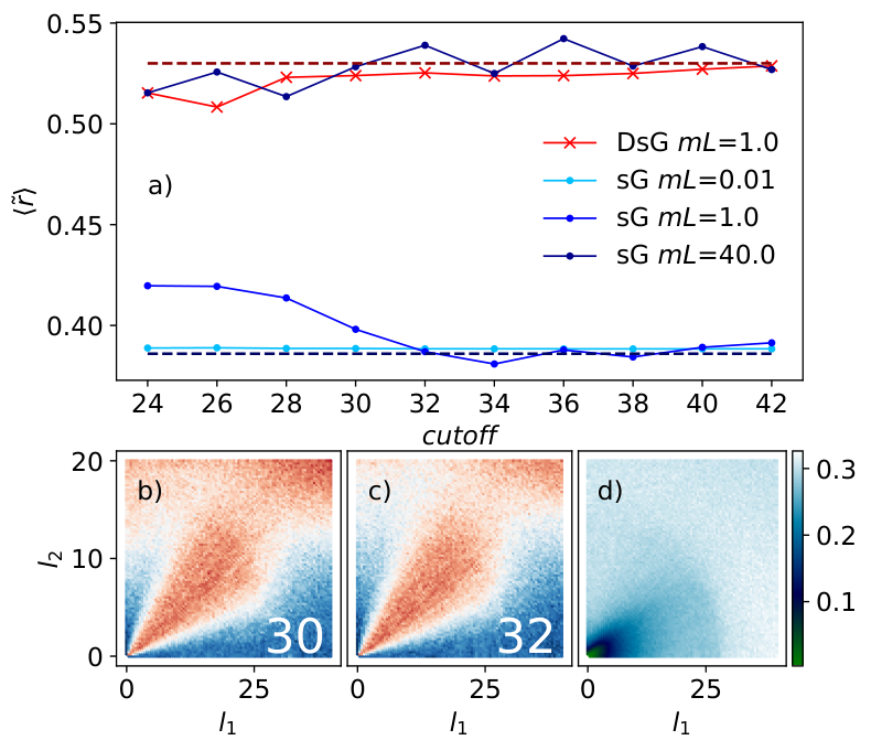
In order to test these statements in an unbiased way, we introduce a measure of the truncation error for spectral statistics and check how it varies for increasing cutoff values. The simplest way to estimate the error of the average of a quantity under study at a given cutoff is by averaging the absolute change of each individual contribution from one cutoff to the next. More explicitly, considering the quantity , we define its error estimate as
| (3) |
where the subscript denotes the index of the value and the superscripts denote the two different energy cutoffs and with at which the corresponding values are obtained. The sum is over the energy window under study, and is the number of values in that window. Based on the assumptions of TCSA, the differences should decay in the limit of the cutoff going to infinity, and hence the mean value is expected to be quite accurate as long as we have reached a sufficiently high cutoff .
But there is more to this error estimate, which makes it very reliable. First, is bounded, taking its maximum value when the two spectra under comparison correspond to spectra of independent random matrices. Second, it behaves analogously to the measure of correlation between the two compared spectra (Fig. 7.g–h). More specifically, when increases then the quantity , where is the Pearson coefficient of correlation between the two spectra, also increases. If the spectra change with the cutoff so much that they are not correlated at all, we can say that they are maximally non-convergent. We can then estimate the maximum error by calculating the average error between two uncorrelated random matrices. This can be performed analytically for matrices by deriving the probability density of the error
| (4) |
and finding its mean. The average error can then be calculated to be . We found numerically that this distribution is very general and holds for matrices of sizes at least up to and even for spectra of matrices that differ only by a few additional rows (Fig. 7.i).
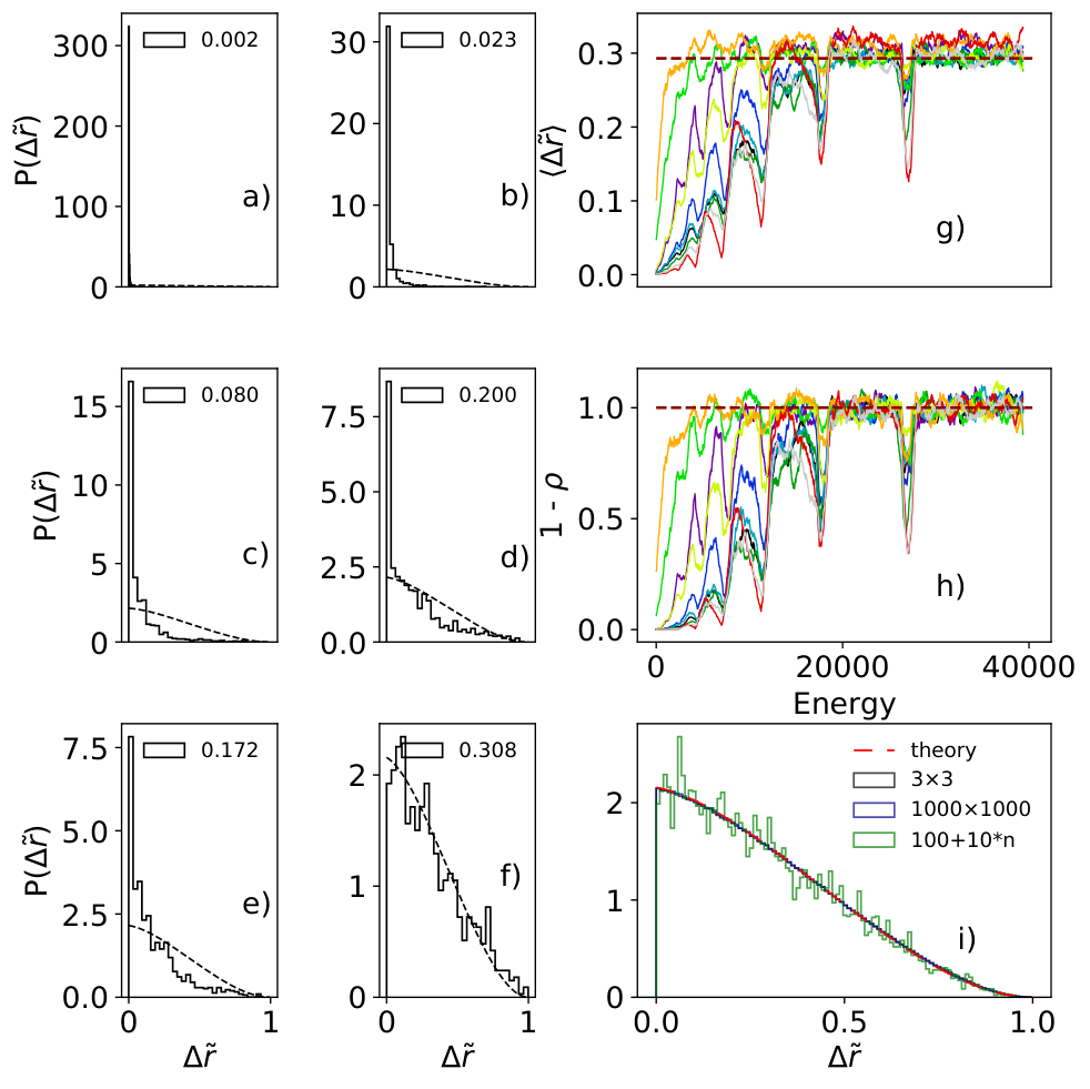
In the models under study we indeed observe that the error estimate is maximal for the least convergent spectra (Fig. 7.g–h). Using this error we can now distinguish between spectra that exhibit RMT-like spectral statistics due to physical reasons or due to truncation artefacts. If the average error is close to the maximum value corresponding to the difference between two uncorrelated random matrices, then the spectra must be random due to non-convergence. If instead we observe very small average errors of the order of, say, of the maximum value, then we can trust that the randomness is due to genuine physical reasons. It should be noted that this measure is still quite conservative, because, as the values are computed from differences of consecutive levels, they are very sensitive to truncation errors and converge much slower than the absolute spectra themselves. Moreover, passing from one cutoff to the next the ordering of a non-negligible number of levels changes, which means that the corresponding differences are larger than the actual values resulting in an overestimation of the error.
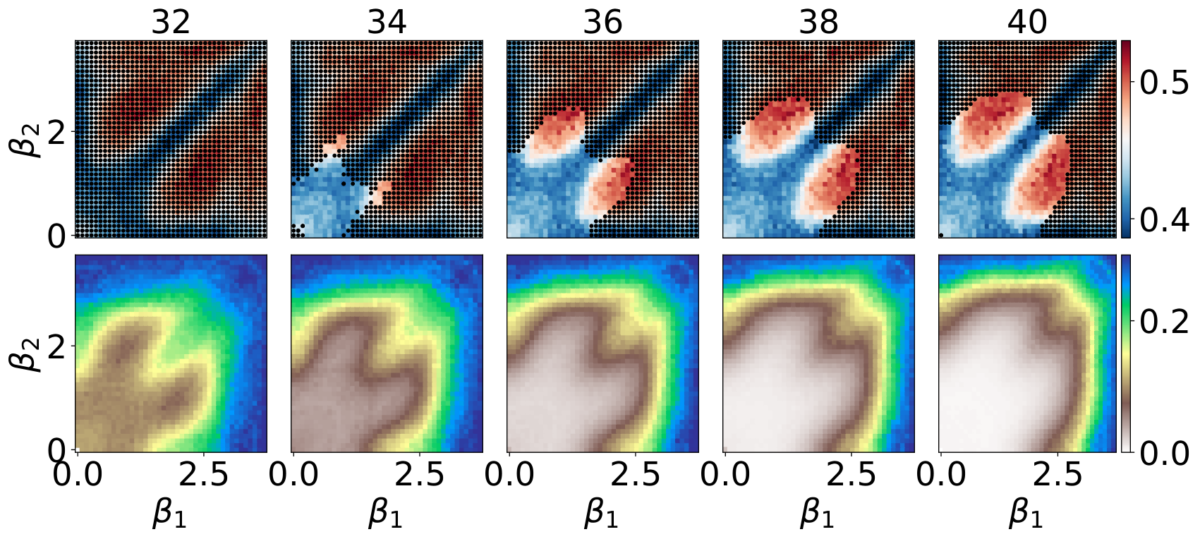
Equipped with a reliable truncation error estimate, we can now test quantitatively the quality of TCSA convergence by analysing how the error changes for increasing values of the cutoff (Fig. 8). We generally find that, when the cutoff goes beyond a sufficiently large value, starts decreasing from the maximum value that it has at lower cutoffs and keeps decreasing while at the same time fluctuating as the cutoff increases further. Based on this convergence tests we find that the best convergence for is achieved in the area around the lower left corner of the phase diagram shown in Fig. 2. Moreover, we find that converges quite well for in the DSG case and in the SG case. Lastly, we verify that convergence is achieved first at lower energy windows (Fig. 7.g–h) with the lowest 3000 to 4000 levels corresponding to well convergent values at in the parameter range of Fig. 2. The spectra and eigenvectors presented in the plots of this paper are sufficiently well convergent with average errors of at most and values of that do not change significantly with the cutoff, unless otherwise stated (Fig. 4, ).
The proposed error measure improves considerably our ability to confidently distinguish physical from numerically artificial results. We now realise that the intuitive guess that non-convergent spectra are RMT-like is not always correct. Even though we do observe that this behaviour is the typical case, we can also clearly find exceptions to this rule: Poisson-like spectral statistics can be observed even in the region with maximal non-convergence (Fig. 6.c).
While we have so far focused on values, we can estimate in a similar way the convergence of eigenvector statistics by comparing how much each eigenvector changes from cutoff to cutoff. We empirically found that a reliable test for the comparison of two vectors can be based on the correlation between their cumulative squared coefficients, which can be used as the fingerprint of a vector. More explicitly, for each numerically computed vector we construct the list for where is the length of the shortest between the two compared vectors, and then compare the two lists by computing the Pearson correlation coefficient. It should be noted in passing that this comparison function is also useful for tracking the eigenvectors as we incrementally change a parameter (physical parameter of the Hamiltonian or the cutoff) and identifying changes in the energy level ordering between two consecutive steps. To this end, we pairwise compare all eigenvectors of one matrix with those of the other and match them based on which pairs show the highest correlation. Typically, such ordering changes are limited to first or second neighbours. In this way we can correct the order of the eigenvectors and therefore obtain a more accurate estimate of the convergence error.
Using this error estimate we found that eigenvector statistics are convergent for a wider range of parameter values than values. This can be easily understood from the fact that the values are more sensitive to small changes in the energy level values. We found that, at the maximum cutoff used here and for the values of as in Fig. 4, eigenvector statistics are well convergent for up to levels at .
.2 Quantum chaos and perturbed CFT
As shown in the main text, the emergence of chaotic level spacing statistics in the DSG occurs already at infinitesimal values of the perturbation strength, as long as the two cosine perturbations are mixed with approximately equal coefficients (Fig. 3.a). This observation motivates us to study the problem using first order perturbation theory. Like any CFT, the spectrum of the free massless boson field theory, which is the unperturbed model, exhibits extensive degeneracies, in which case perturbation theory tells us that at first order the perturbation affects each of the degenerate energy shells independently from the others. This means that at first perturbative order we can analyse the spectral statistics working on finitely dimensional Hilbert spaces (those of the degenerate energy shells), that is, without having to deal with the problems arising from an infinite Hilbert space dimension and the need to truncate it in an efficient way. This is especially convenient as it allows us to derive exact spectra and statistics, reach higher energy shells and study the changes in spectral statistics for increasing shell number. In this appendix, we present more detailed results for the statistics of level spacings and eigenvectors of the DSG model at first order in perturbation theory.
The Hamiltonian of the free massless boson field theory with Dirichlet boundary conditions is (up to an irrelevant additive constant)
| (5) |
where are the ladder operators corresponding to the sinusoidal harmonic eigenfunctions with wavenumbers , satisfying canonical commutation relations , and the single particle dispersion relation is (in units where the speed of light is and ). The eigenstates of are therefore
| (6) |
with eigenvalues
| (7) |
Evidently, owing to the linearity of the dispersion relation, all energy eigenvalues of are integer multiples of and can be classified into shells of degenerate levels with energy for all positive integers and degeneracy equal to the number of integer partitions of . For large the number increases rapidly (). For this reason the dimensions of CFT degenerate shells increase with the energy faster than in few-body quantum mechanical systems (e.g. hydrogen atom). We will denote the subspace corresponding to the shell with energy as . Taking into account the additional restriction to a single symmetry sector (see Sec. .3), the resulting shell sizes are listed in Tab. 1.
| shell no. | number of states | |
|---|---|---|
| 10 | 22 | 505 |
| 11 | 24 | 793 |
| 12 | 26 | 1224 |
| 13 | 28 | 1867 |
| 14 | 30 | 2811 |
| 15 | 32 | 4186 |
| 16 | 34 | 6168 |
| 17 | 36 | 9005 |
Let us consider a perturbation of by an operator that raises the degeneracy of the energy levels at first order in the perturbation parameter . This is true for the DSG interaction. From degenerate perturbation theory we know that the perturbed energy eigenstates of corresponding to the shell are
| (8) |
with energy eigenvalues
| (9) |
where and are the eigenvectors and corresponding eigenvalues of the restriction of in the subspace . In the limit the perturbed eigenstates are linear combinations of states of the shell they originate from and only those. We will therefore focus on the eigenvectors and eigenvalues of whose statistics are identical to those of in the subspace as . In the case of the DSG model, therefore in the above limit the spectrum is a function of the mixing parameter . For or the model reduces to the SG.
In the following we will analyse the dependence of spectral statistics on the mixing parameter and shell number , keeping and fixed at the values used in the main text, i.e. 1 and 2.5 respectively. Fig. 9 shows histograms of based on in-shell spectra for the 17th shell () at various values of the mixing parameter, demonstrating the transition from Poisson statistics at to GOE at where is maximal. Owing to the larger spectrum size, the statistical fluctuations of the histograms are reduced compared to Fig. 1 of the main text, allowing a more accurate comparison with the theoretical curves. In Fig. 10.a showing as a function of in different shells, it is evident that as we move from lower to higher shells, approaches the GOE value closer and in a broader window of values expanding from the middle . This suggests that at higher energy levels the RMT behaviour of level spacings not only persists but also becomes more prominent. In-shell eigenvector statistics exhibit identical scaling as that shown in Fig. 4 in the main text, which is computed from spectra at intermediate values of the perturbation strength.
As pointed out in the main text, the above general features of spectra and eigenvectors observed in the limit persist for all values of the perturbation parameters for which convergence was achieved in our study. Fig. 11 shows that the spectra exhibit a distinct shell structure characteristic of first-order perturbation theory for all , while the shells start sensing each other at and visibly mix with each other at larger . In particular, at the maximum value for which we have achieved convergence of the spectrum and eigenvectors (lowest levels), the effects of the interaction are strong enough to result in a spectral density that is clearly different from that of first-order perturbation theory. Yet the level spacing and eigenvector statistics for exhibit the same characteristics as for .
.3 Details of the Hamiltonian Truncation Method
As mentioned in the main text, Hamiltonian truncation methods have been extensively used for the derivation of the spectra of almost all of the models studied in the present work. Details on the application of TCSA to SG and DSG can be found in Feverati et al. 1998; Feverati et al. 1999; Fehér and Takács 2011; Kukuljan et al. 2018 and Bajnok et al. 2001; Takács and Wágner 2006 respectively, while the application to MSG is a relatively straightforward extension of the method. Details on Hamiltonian truncation in the model can be found in Hogervorst et al. 2015; Rychkov and Vitale 2015; Rychkov and Vitale 2016; Elias-Miró et al. 2017. Here we provide further information relevant for the analysis of spectral statistics in these models. More specifically, we discuss the discrete symmetries of the models and restriction to a single symmetry sector, provide information on the size of the truncated bases we used and hints on the efficient construction of the Hamiltonian matrices. Lastly, we give explicit formulas for the parameters of the models as used here.
Massless free boson basis
We express the SG, DSG and MSG Hamiltonians in the truncated free boson CFT eigenstate basis ordering the states by their energy. We assume Dirichlet boundary conditions in a box of length . Both the unperturbed and perturbed Hamiltonians are invariant under two discrete transformations: field reflection and space reflection . For the study of spectral statistics it is necessary to eliminate any symmetries of the model by restricting the spectrum to a single symmetry sector (energy levels belonging to different symmetry sectors are independent and can clearly cross with each other). Out of the four symmetry sectors we choose the one containing the ground state. The truncated basis sizes of the selected symmetry sector are listed in Tab. 2. The Hamiltonian matrix is dense in this basis and to derive the spectra we use exact diagonalisation. The construction time of the Hamiltonian matrix can be reduced considerably using simple parallelisation.
| cutoff | number of states | CPU time [days] |
|---|---|---|
| 32 | 12170 | 0.7 |
| 34 | 18338 | 2 |
| 36 | 27343 | 4 |
| 38 | 40369 | 8 |
| 40 | 59061 | 17 |
| 42 | 85674 | 36 |
Klein Gordon basis
To achieve sufficiently good convergence the Hamiltonian should be expressed in the KG instead of the massless free boson basis Hogervorst et al. 2015; Bajnok and Lajer 2016. The perturbation operator (more generally any operator) is sparse in this basis, and so the construction of the corresponding matrix can be programmed efficiently with the use of dictionaries associating each basis state with its order in the basis. This way we can benefit from the logarithmic lookup time and considerably speed up the calculation. For easier comparison with earlier literature Hogervorst et al. 2015; Bajnok and Lajer 2016 we focused on the case of periodic boundary conditions. This means that we now have translational invariance symmetry, apart from the symmetry under field reflection . We again restrict ourselves to a single symmetry sector, the one containing the ground state. For the basis truncation we set the total momentum cutoff at 42 and the system size is chosen to be , where is the KG mass parameter. This choice corresponds to a basis size of . To compute the spectra and eigenstates of the Hamiltonian, we employed sparse matrix diagonalisation techniques, which allowed us to obtain the lowest eigenvalues and eigenstates.
Construction of the SG, DSG and MSG Hamiltonian matrices
The free boson CFT Hamiltonian for a system of length with Dirichlet boundary conditions, expressed in dimensionless form in units of a mass scale , is
| (10) |
where . The sine-Gordon Hamiltonian is defined as
| (11) |
with
| (12) |
where
| (13) |
is the vertex operator. As in the standard TCSA notation, the perturbation strength has been re-parametrised in favour of the first sine-Gordon breather mass in units of the inverse system size , which is equal to the energy gap between the ground and first excited state in the thermodynamic limit
| (14) |
where
| (15) | ||||
| (16) |
and
| (17) |
is the first breather mass, where is the soliton mass.
To construct the double sine-Gordon Hamiltonian with frequencies and , we add the corresponding sine-Gordon Hamiltonians. More explicitly, when we vary we adjust the coefficients so as to keep the values of fixed and equal , and compute the spectra of the dimensionless Hamiltonian matrix
When we vary and at fixed and (Fig. 6), we use the Hamiltonian matrix
When studying the massive Schwinger-Thirring model, we write the Hamiltonian as
.4 DSG spectral statistics in subsets of states within one shell
To investigate the inner structure of the energy shells of the DSG model presented in the main text (Fig. 4), we focus on a single shell, divide it into non-overlapping subsets of increasing energy levels and analyse the statistics of eigenvector components in each of the subsets. This way we can check whether the observed deviation of the eigenvector component statistics from RMT is due to the existence of a small number of non-typical eigenstates concentrated at the edges of the shell or if it is a general characteristic of the majority of the eigenstates. As a measure of randomness of the eigenvectors , we also compute the entropy . The maximum value of the entropy corresponds to a vector with all components equal (where is the length of the vector). The expectation value of the entropy of a random vector in GOE is for large Kota 2014.
The results are shown in Fig. 12. We observe that the eigenstates close to the edges of the shell exhibit less random characteristics. The mean eigenvector entropy is lower than in the middle of the shell, and also has a lower value at the low energy edge. Moreover, there are variations in the distribution of eigenvector components. In contrast to the middle of the shell, the edges are characterised by non-exponential scaling in the bulk of the distribution and a higher peak at zero. However, the tails of the distributions are clearly non-Gaussian in all subsets independently of their position in the shell. We have verified that the same holds for different parameter values and different shells. We thus conclude that the deviations from RMT predictions are present in the full energy range of each shell, and they are not caused by a small number of non-typical eigenstates.