The combinatorial PT-DT correspondence
Abstract
We resolve an open conjecture from algebraic geometry, which states that two generating functions for plane partition-like objects (the "box-counting" formulae for the Calabi-Yau topological vertices in Donaldson-Thomas theory and Pandharipande-Thomas theory) are equal up to a factor of MacMahon’s generating function for plane partitions. The main tools in our proof are a Desnanot-Jacobi-type "condensation" identity, and a novel application of the tripartite double-dimer model of Kenyon-Wilson.
keywords
Plane partitions, double-dimer model, Desnanot-Jacobi identity, Donaldson-Thomas theory, Pandharipande-Thomas theory1 Introduction
Donaldson-Thomas (DT) theory and Pandharipande-Thomas (PT) theory are branches of enumerative geometry closely related to mirror symmetry and string theory. In both theories, generating functions arise known as the combinatorial Calabi-Yau topological vertices. These generating functions enumerate seemingly different plane partition-like objects. In this paper, we prove that the generating functions coincide up to a factor of , MacMahon’s generating function for plane partitions [Mac16]. Our result, taken together with a substantial body of geometric work, proves a geometric conjecture in the foundational work of Pandharipande-Thomas theory which has been open for over 10 years.
The generating function from Donaldson-Thomas theory is known as the DT topological vertex. Denoted , where each is a partition, it counts plane partitions asymptotic to , and (see Section 3.1). The PT topological vertex, denoted by , is a generating function for a certain class of finitely generated -modules (see Section 4.1).
We prove that
Theorem 1.
The geometric corollary of this theorem is a proof of Theorem/Conjecture 2 of [PT09], which, loosely speaking, states that computes the local contribution to the Pandharipande-Thomas generating function. The proof of this corollary combines Theorem 1 with the analogous result in DT theory [MNOP06a, MNOP06b, MPT10] along with [MOOP11, Section 4.1.2]; it is a consequence of the fact that both DT and PT theory give the same invariants as a third theory, Gromov-Witten theory.11 1 In [PT09, MNOP06a, MNOP06b] and in general elsewhere in the geometry literature, all of the formulas have replaced by . The sign is there for geometric reasons which are immaterial for us.
The combinatorics problems which we solve are stated in the geometry literature as “box-counting” problems; that is, the objects of interest are plane partition-like. The following bijections are well-known:
The first one is a 3D version of the correspondence between a partition and its Maya diagram; it is stated explicitly in Section 3.2. We use essentially the same correspondence to give a dimer description of the DT topological vertex . On the PT side, the correspondences are
The correspondence (1) is new, as far as we are aware. We describe labelled box configurations, and the generating functions for them which arise in PT theory, carefully in Section 4. Interestingly, though it is a purely combinatorial correspondence, it is not bijective—rather, it is a weight-preserving, 1-to-many correspondence. Here is spanned by all monomials where and ranges over some fixed partition , with defined similarly; the quotient is killing the diagonal of the direct sum.
The correspondence (2) is incidental to this work and is described in [PT09]; nor will we need to discuss the structure of the modules in the codomain. We expect that our methods will be relevant in other similar situations (one such situation arises in Rank 2 DT theory [GKY18]) and we would be eager to learn of other instances in which our techniques would apply.
We prove Theorem 1 by observing that both and are the unique solution of the same recurrence, with the same initial conditions. The recurrence in question is called the condensation recurrence; we postpone its definition to Section 2, after we have made the required definitions.
Viewed as a recurrence in and , Equation (2) uniquely characterizes and . The base case is when one of the three partitions is equal to zero; Equation (1) is known to hold in this situation [PT09].
When recast in terms of the dimer model, is easily seen to satisfy Equation (2) by Kuo’s graphical condensation [Kuo04]; this is essentially the content of Section 3.
Showing that satisfies Equation (2) is considerably more intricate, but once we translate to the double-dimer model, the bulk of the work was done elsewhere, in work of Jenne [Jen20]. Essentially, [Jen20] evaluates a certain determinant by the classical Desnanot-Jacobi identity, and then interprets all six terms in the identity in terms of .
The full version of this abstract will appear in [JWY]; proofs have been omitted due to space constraints.
2 Definitions
Fix partitions . For this paper, we identify with the coordinates of the boxes of its Young diagram, with the corner of the diagram located at . Define the following subsets of , thought of as sets of boxes: , and
Moreover, let denote the integer points in the first octant (including the coordinate planes and axes). Let and . Finally, let
| I I | |||||||
| I I I | |||||||
We will need the following standard notions of Maya diagrams. If is a partition with parts, define for . The Maya diagram of is the set . We frequently associate a partition with its Maya diagram by drawing a Maya diagram as a doubly infinite sequence of beads and holes, indexed by , with the beads representing elements of the above set. For instance, the Maya diagrams of the empty partition and of the partition are the sets and , respectively, which are drawn as
When convenient, we simply mark the location of 0 with a vertical line, rather than labelling the beads with elements of . Conversely, if is a subset of , define and . If both and are finite, then define the charge of , , to be ; then it is easy to check that the set is the Maya diagram of some partition ; we say that itself is the charge Maya diagram of .
If is a partition with Maya diagram , let (resp. ) be the partition associated to the charge (resp. ) Maya diagram (resp. ). Let be the partition associated to the Maya diagram .

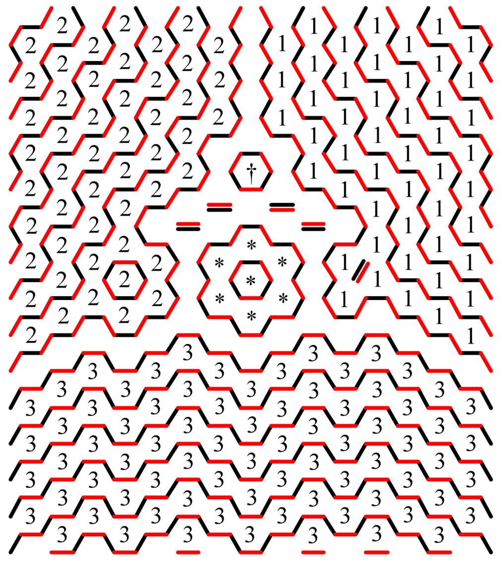
In both PT and DT, it will be convenient to divide the honeycomb graph into three sectors and label some of the vertices on the outer face as shown in Figure 1 for . We remark that the division into sectors makes sense as . The reason for these particular choices of labels is that we will need to specify these specific vertices, both in DT and PT, based on the Maya diagrams of various partitions.
Finally, let be a power series in , depending on three partitions , which is symmetric with respect to cyclic permutation of these partitions. We shall be interested in solutions to the following functional equation:
| (2) |
Here, are certain explicit constants depending on which we don’t define in this extended abstract. These constants are discussed further in Section 3.3.
Since the partitions , , are all smaller, in some sense, than , and since none of the topological vertex terms are equal to zero, we can divide both sides of the condensation recurrence by and obtain a recursive characterization of . Note also that by symmetry - so we can say that is the unique power series which satisfies the condensation recurrence, where we take the base cases to be the (known) value of for all partitions .
3 DT
3.1 DT box configurations
We say that a plane partition asymptotic to () is an order ideal under the product order in which contains , together with only finitely many other points in . We let denote the set of plane partitions asymptotic to .
If any of are nonzero, then every is an infinite subset of . We define the customary measure of “size” of such a plane partition in the geometry literature (see, for instance, [MNOP06a]).
Define
We call the topological vertex in Donaldson-Thomas theory. Note that if with , then is a plane partition of in the conventional sense, that is, a finite array of integers such that each row and column is a weakly decreasing sequence of nonnegative integers. Thus MacMahon’s enumeration of plane partitions [Mac16] gives us .
3.2 DT theory and the dimer model
Before giving the dimer description of , we review the correspondence between plane partitions and dimer configurations of a honeycomb graph. By representing each integer in a plane partition as a stack of unit boxes, a plane partition can be visualized as a collection of boxes which is stacked stably in the positive octant, with gravity pulling them in the direction . This collection of boxes can be viewed as a lozenge tiling of a hexagonal region of triangles, which is equivalent to a dimer configuration (also called a perfect matching) of its dual graph.
Just as a plane partition can be visualized as a collection of boxes, a plane partition asymptotic to can be visualized as a collection of boxes, as shown in Figure 2, left picture. Moreover, a version of the above correspondence puts these box collections in bijection with dimer configurations on the honeycomb graph with some outer vertices removed, which we call . Specifically, is constructed as follows. Let be the Maya diagram of . Construct the sets , for and then remove the vertices with the labels in from sector of (here, we are referring to the labelling of the boundary vertices illustrated in Figure 1, left picture).

3.3 The condensation recurrence in DT theory
We now show that the DT partition function satisfies the condensation recurrence; this is now a corollary of the well-known “graphical condensation” theorem of Kuo:
Theorem 2.
[Kuo04, Theorem 5.1] Let be a planar bipartite graph with a given planar embedding in which . Let vertices and appear in a cyclic order on a face of . If and , then
Take to be for sufficiently large22 2 A sufficient lower bound for depends on , , and .. Let and be the vertices in sector 1 labelled by and , respectively. Similarly, we let and be the vertices in sector 2 labelled by and . Then is .
The resulting six dimer-model partition functions are all instances of the topological vertex, up to order . The normalization constants arise because the “folklore” technique which associates a plane partition to a dimer configuration preserves the weight up to a factor of , where is the minimal dimer configuration. The weight of this configuration is computed, for instance in [Kuo04]; for us the computation is substantially messier, as depends on in a delicate way; we omit the details.
4 PT
4.1 Labelled configurations
In this section we introduce one of the main objects of our study: labelled configurations.
Definition 1.
If and are finite sets of boxes, then is an configuration if the following condition is satisfied:
-
If is a cell in (resp. ) and any cell in supports a box in (resp. ), then must support a box in (resp. ).
We remark that this is the familiar condition for plane partitions, except that gravity is pulling the boxes in the direction , away from the origin.
Next, we give an algorithm that labels configurations. Note that the algorithm assigns labels to cells, not boxes.
Algorithm 1.
- 1.
If a connected component of contains a box in and a box in , where , terminate with failure.
- 2.
For each connected component of that contains a box in , label each element of by .
- 3.
For each remaining connected component of , label each element of by the same freely chosen element of .
Because the algorithm may fail in Step 1, there are configurations that cannot be labelled. A labelled configuration is an configuration for which the labelling algorithm succeeds. Let denote the set of all labelled configurations.


Example 1.
Let and . Then and . In Figure 3 we illustrate four configurations33 3 The first three of these configurations appear in [PT09, Section 5.4] as the length 1 configuration (i), the length 3 configuration (iv), and the length 2 configuration (iii)., three of which are labelled configurations.
- 1.
consists of a single box at and . Step 2 of Algorithm 1 gives the cells and the label 1, which is indicated by the color purple. The cell is opaque because it supports a box; the cell does not.
- 2.
and . Step 2 labels the cells in by 3, which we illustrate by coloring the two boxes cyan. The box at is colored gray because it does not get a label.
- 3.
and . Again, the box at does not get a label. The box at has a free choice of label in .
- 4.
and . The algorithm terminates with failure in Step 1 because and . In the figure, is colored both cyan, required by the box at , and purple, required by the cell at .


Example 2. Figure 4 shows a labelled configuration with and . The left image shows the configuration. The boxes belonging to are marked; all other boxes are in . The right image includes surrounding cells in I I. In both images, yellow cells are labelled 2 and purple cells are labelled 1. Opaque cells support a box in the configuration and transparent cells do not. The two connected components labelled by a freely chosen element of are colored black and orange, respectively.
Define
We prove, in a paper in preparation, that labelled configurations are a discrete version44 4 More precisely, there is a surjection from labelled configurations to labelled box configurations, and if is a labelled box configuration, , where is the topological Euler characteristic of the moduli space of labellings of , in the terminology of [PT09]. of labelled box configurations as defined in [PT09, Section 2.5], and therefore is the topological vertex in PT theory.
4.2 PT theory and the labelled double-dimer model
Next we explain the relationship between labelled configurations and double-dimer configurations. On an infinite graph, a double-dimer configuration is the union of two dimer configurations.
Let be an configuration. We consider and separately. For , we view the surface as a lozenge tiling. In other words, we take the set of boxes and draw the tiles corresponding to cells that are not in . Similarly, for , we view the surface as a lozenge tiling. We then extend each of these tilings to tilings of the entire plane. That is, in Figure 5, we overlay the third image on the second image to obtain the final image. Then, these lozenge tilings are equivalent to dimer configurations of the infinite honeycomb graph .
Let (resp. ) denote the dimer configuration of corresponding to the infinite tiling obtained from (resp. ). Superimposing and so that Region I I I is in the same place in the two pictures produces a double-dimer configuration on .
For example, the third image of Figure 5 shows the tiling corresponding to , where is the configuration from Figure 4. The set consists of two boxes, and , so we have drawn the tiles corresponding to .
The corresponding dimer configurations and are shown in Figure 6. Their superposition, shown immediately to their right, is a double-dimer configuration on .
Just as we label certain configurations, we label certain double-dimer configurations. Before presenting our double-dimer labelling algorithm, we make a few remarks. It can be shown that each path in crosses each coordinate axis finitely many times. Consequently, there is a well-defined notion of the sectors55 5 When we refer to “sectors” in this section, we mean the sectors defined in the right hand side of Figure 1. that contain the ends of such a path. Also, let be the relative height function that assigns to each face of the height difference at of the surface corresponding to above that corresponding to . The loops and paths in are the contour lines for . Every path in divides the plane into two disjoint regions, and we call such a region the higher side of the path if increases by when entering that region by crossing the path.
Algorithm 2.
- 1.
If contains a path whose ends are contained in different sectors, terminate with failure.
- 2.
For each path in such that sector contains the ends of that path, label each face of contained in the higher side of that path by .
- 3.
For each loop in that is not contained in the interior of another loop or the higher side of a path, label each enclosed face of by the same freely chosen element of .
For example, if we label the double-dimer configuration from Figure 6, we obtain the labelled double-dimer configuration shown in Figure 6. Observe that the paths in the double-dimer configuration in Figure 6 are “rainbow-like.” In other words, the paths are nested and start and end in the same sector.
Theorem 3.
Let be an configuration. Then is a labelled configuration if and only if the double-dimer configuration has the property that each path starts and ends in the same sector.
In order to apply the double-dimer analogue of Kuo’s graphical condensation, we must truncate our double-dimer configuration on the infinite honeycomb graph to obtain a double-dimer configuration with nodes on the honeycomb graph .
Definition 2.
Let be a finite edge-weighted bipartite planar graph embedded in the plane with . Let denote a set of special vertices called nodes on the outer face of . A double-dimer configuration on is a multiset of the edges of with the property that each internal vertex is the endpoint of exactly two edges, and each vertex in is the endpoint of exactly one edge.
Each double-dimer configuration is associated with a planar pairing of the nodes. On a finite graph, the notion that the paths are “rainbow-like” means that the pairing is tripartite.
Definition 3.
A planar pairing is tripartite if the nodes can be divided into three circularly contiguous sets , and so that no node is paired with a node in the same set. We often color the nodes in the sets red, green, and blue, in which case is the unique planar pairing in which like colors are not paired.

The process of truncating the infinite double-dimer configuration is straightforward and details are omitted here. Continuing our example, truncating the double-dimer configuration from Figure 6 to a double-dimer configuration on produces the tripartite double-dimer configuration shown in Figure 7.
The set of nodes N and the coloring of these nodes is determined by the partitions , and , and this can be made explicit by using the Maya diagram associated to each partition.
We refer to the labelling and sectors of the graph shown in Figure 1.
To determine the nodes in Sector , we draw the Maya diagram associated to .
- •
In Sector 1, the blue nodes are the holes with positive coordinates and the red nodes are the beads with negative coordinates.
- •
In Sector 2, the red nodes are the holes with positive coordinates and the green nodes are the beads with negative coordinates.
- •
In Sector 3, the green nodes are the holes with positive coordinates and the blue nodes are the beads with negative coordinates.
4.3 The condensation identity for PT invariants
Let denote the weighted sum of all double-dimer configurations with a particular pairing . In [Jen20], the first author showed that when is tripartite and certain other technical conditions hold we have the following:
We apply this recurrence by adding nodes to the graph so that for four nodes , , and . We choose the four nodes as follows: Let and be the nodes in sector 1 labelled by and , respectively. Similarly, we let and be the nodes in sector 2 labelled by and . Note that these nodes have the same coordinates as the vertices specified in Section 3.3 but the coordinate system is different (see Figure 1). Many details here have been omitted, due to space constraints.
Acknowledgements.
We would like to thank Jim Bryan, Rick Kenyon, Rahul Pandharipande, Richard Thomas, Jim Propp, Karel Faber, Kurt Johansson, and frankly countless other geometers, probabilists and combinatorialists for helpful conversations.References
- [GKY18] Amin Gholampour, Martijn Kool, and Benjamin Young. Rank 2 Sheaves on Toric 3-Folds: Classical and Virtual Counts. Int. Math. Res. Not. IMRN, (10):2981–3069, 2018.
- [Jen20] Helen Jenne. Combinatorics of the Double-Dimer Model. PhD thesis, University of Oregon, 2020.
- [JWY] Helen Jenne, Gautam Webb, and Ben Young. The combinatorial PT-DT correspondence. In preparation.
- [Kuo04] Eric H Kuo. Applications of Graphical Condensation for Enumerating Matchings and Tilings. Theoretical Computer Science, 319(1-3):29–57, 2004.
- [Mac16] P. A. MacMahon. Combinatory Analysis. Cambridge University Press, Cambridge, UK, 1915-16.
- [MNOP06a] Davesh Maulik, Nikita Nekrasov, Andrei Okounkov, and Rahul Pandharipande. Gromov–Witten theory and Donaldson–Thomas theory, I. Compositio Mathematica, 142(5):1263–1285, 2006.
- [MNOP06b] Davesh Maulik, Nikita Nekrasov, Andrei Okounkov, and Rahul Pandharipande. Gromov–Witten theory and Donaldson–Thomas theory, II. Compositio Mathematica, 142(5):1286–1304, 2006.
- [MOOP11] D Maulik, Alexei Oblomkov, Andrei Okounkov, and Rahul Pandharipande. Gromov-Witten/Donaldson-Thomas correspondence for toric 3-folds. Inventiones Mathematicae, 186(2):435–479, 2011.
- [MPT10] Davesh Maulik, Rahul Pandharipande, and Richard P Thomas. Curves on K3 surfaces and modular forms. Journal of Topology, 3(4):937–996, 2010.
- [ORV06] Andrei Okounkov, Nikolai Reshetikhin, and Cumrun Vafa. Quantum Calabi-Yau and Classical Crystals. In The Unity of Mathematics, Volume 244 of Progr. Math., pages 597–618. Birkhäuser Boston, Boston, MA, 2006.
- [PT09] Rahul Pandharipande and Richard P Thomas. The 3–fold vertex via stable pairs. Geometry & Topology, 13(4):1835–1876, 2009.