跳到论文正文
W Papers独立论文阅读器 arXiv:2012.08473 论文正文 计算阅读时间 · 0%
引用这篇论文根据当前论文元数据生成,正式投稿前建议核对。


License: CC BY 4.0
arXiv:2012.08473v1 [math.DG] 15 Dec 2020

Acknowledgements

There are several people I would like to thank for helping me get to this thesis.

Vorrei ringraziare con affetto Francesco Bonsante che, con molta disponibilità, ha accettato tre anni fa di farmi da tutor per il dottorato. È stato una guida illuminante, paziente e generosa e gli sarò sempre grato per avermi insegnato a camminare nel mondo della ricerca.

Vorrei ringraziare Andrea Seppi, il mio "fratello maggiore" accademico, che ha investito tempo e pazienza per collaborare con un principiante. Insieme abbiamo trovato un po’ di matematica interessante e io ho trovato un buon amico.

I would like to thank Jean-Marc Schlenker for offering me a postdoc position in a tough moment for the academic job market. I thank him for his kindness and for the interesting conversations that we had and that we will have in Luxembourg.

Un grazie profondo ai miei genitori. Mi hanno sempre lasciato libero di vivere il mio percorso e di fare le mie scelte (anche se forse a volte preferirebbero un figlio impiegato di banca che abiti a cinque minuti da casa). Vi voglio tanto bene e, anche quando non ci sono, sono sempre lì.

Un grazie amorevole a Silvia, che accetta con pazienza di vivere una relazione quasi costantemente a distanza, ma che offre sempre ristoro al mio cuore vagabondo e che mi porta una casa ogni volta che mi viene a trovare.

Ringrazio con tantissimo affetto tutti i miei compagni di dottorato. Grazie per le risate, per i pranzi, le pause tè e caffè per tutte le tante minipause fittamente distribuite durante il lavoro. È stato un bellissimo percorso di crescita condivisa, avete reso questi tre anni i più belli della mia formazione.

Un grazie anche ai miei amici Miriam, Niyi, Oreste, Giorgio, Lorenzo, Martina, Rossana, il prof. Monti, Gabriele, Eugenia - e ne sto dimenticando qualcuno - per essere sempre una buona ragione in più per tornare a casa.

Being independent is beautiful, but always having someone to thank is probably even more so.

Chapter 1 Introduction

It is a well known result in Riemannian and Pseudo-Riemannian Geometry that the theory of codimension-1 (admissible) immersions of a simply connected manifold MM into a space form is completely described by the study of two tensors on MM, the first fundamental form and the shape operator of the immersion, corresponding respectively to the pull-back metric and to the derivative of a local normal vector field.

On the one hand, for a given immersion the first fundamental form and the shape operator turn out to satisfy two equations known as Gauss and Codazzi equations. On the other hand, given a metric and a self-adjoint (1,1)-tensor on MM satisfying these equations, there exists one admissibile immersion into the space form with that pull-back metric and that self-adjoint tensor respectively as first fundamental form and shape operator; moreover, such immersion is unique up to post-composition with ambient isometries of the space form. This class of results are often denoted as Gauss-Codazzi Theorems, Bonnet Theorems or as Fundamental Theorem of hypersurfaces, and can be extended for higher codimension. See for instance [KN96, LTV10]. We will recall in Chapter 2 the Gauss-Codazzi theorems for pseudo-Riemannian space forms of constant sectional curvature −1-1, such as ℍn\mathbb{H}^{n} and A​d​Sn~\widetilde{AdS^{n}}.

Several remarkable results in the study of geometric structures on surfaces have been developed from the study of immersions of surfaces into ℍ3\mathbb{H}^{3} and A​d​S3AdS^{3}. A convex equivariant immersion of S~\widetilde{S} into ℍ3\mathbb{H}^{3} induces a projective structure on SS with developing map defined by the immersion Gσ+:S~→∂ℍ3G^{+}_{\sigma}\colon\widetilde{S}\to\partial\mathbb{H}^{3} with Gσ+​(p)G_{\sigma}^{+}(p) being the endpoint of the geodesic ray starting at σ⁡(p)\sigma(p), orthogonal to σ\sigma and directed toward the concave side: this has been a starting point for several results about projective structures [Lab92, BMS13]. On the other hand, the Gauss map of an equivariant Riemannian immersion of S~\widetilde{S} into A​d​S3AdS^{3} points out a pair of points in the Teichmüller space of SS and minimal isometries are related to the problem of finding minimal Lagrangian maps between hyperbolic metrics, see [KS07, BS10].

In this thesis, we present two possible developments for this theory of immersions.

  • •

    Immersions of smooth manifolds into holomorphic Riemannian space forms of constant curvature −1-1, that we will denote as 𝕏n+1\mathbb{X}_{n+1} (see Subsection 1.1.1, complete definition in Chapter 3).

    A proper definition of holomorphic Riemannian metric (and of corresponding Levi-Civita connection and curvature) will be given in Chapter 3 (see Definition 3.1.1). Let us just mention now that holomorphic Riemannian metrics are a natural analogue of Riemannian metrics in the complex setting, and that holomorphic Riemannian space forms are simply-connected complex manifolds endowed with a holomorphic Riemannian metric with the property of being complete and with constant sectional curvature.

    The theory of immersions into 𝕏n+1\mathbb{X}_{n+1} generalizes the one of immersions into hyperbolic pseudo-Riemannian space forms, since they all isometrically immerge into 𝕏n+1\mathbb{X}_{n+1}, leading to a more general version of the Gauss-Codazzi Theorem.

    This approach also allows to furnish a tool for constructing holomorphic variations of projective structures, with connections with the complex landslide. Moreover, this theory leads to the definition of a new geometric structure for surface, namely complex metrics, for which we state a uniformization theorem that is deeply connected with Bers Simultaneous Uniformization Theorem. For n=3n=3, we see that the space 𝕏3\mathbb{X}_{3} is isometric to SL⁡(2,ℂ){\mathrm{SL}(2,\mathds{C})} equipped with the global complex Killing form, up to a scalar.

  • •

    Immersions of smooth nn-manifolds into the space 𝔾n+1\mathbb{G}_{n+1} of the geodesics of ℍn+1\mathbb{H}^{n+1}.

    In general an immersion σ\sigma of a hypersurface M=MnM=M^{n} in ℍn+1\mathbb{H}^{n+1} induces a Gauss map Gσ=(Gσ+,Gσ−)G_{\sigma}=(G_{\sigma}^{+},G_{\sigma}^{-}) into its space of geodesics, identified with ∂ℍn+1×∂ℍn+1∖Δ=:𝔾n+1\partial\mathbb{H}^{n+1}\times\partial\mathbb{H}^{n+1}\setminus\Delta=:\mathbb{G}_{n+1}, defined by taking, at each point, the endpoints of the normal oriented unparametrized geodesic to σ\sigma. If σ\sigma has principal curvatures in (−1,1)(-1,1), both Gσ+G_{\sigma}^{+} and Gσ−G_{\sigma}^{-} are developing maps for projective structures.

    The space 𝔾n\mathbb{G}_{n} has an interesting para-Kähler structure (see Section 5.2) which encodes a lot of geometric aspects of the hyperbolic space.

    In this thesis we mainly question when an immersion G:Mn→𝔾n+1G\colon M^{n}\to\mathbb{G}_{n+1} is the Gauss map of an immersion into ℍn+1\mathbb{H}^{n+1}, distinguishing among local, global and equivariant integrability: in this sense we provide a characterization for integrability of Riemannian immersions in terms of their extrinsic geometry in relation with the para-Kähler structure of 𝔾n+1\mathbb{G}_{n+1}. We will also focus on the symplectic geometry of 𝔾n+1\mathbb{G}_{n+1} and of (equivariant) Hamiltonian symplectomorphisms of this space, which turn out to send (equivariantly) integrable immersions into (equivariantly) integrable immersions.

These two subjects have at least one point of contact: indeed, the space of geodesics of ℍ3\mathbb{H}^{3} has a structure of holomorphic Riemannian space form of constant curvature −1-1.

This thesis draws its content mainly from the papers [BE20] and [ES20], in which I have been working on together with Francesco Bonsante and Andrea Seppi respectively, jointly with some unedited contents and remarks.

After the Introduction chapter, the thesis will proceed with the following structure.

  • •

    Part I is mainly devoted to the presentation of the spaces 𝕏n\mathbb{X}_{n} and 𝔾n\mathbb{G}_{n}. The part will start with a short chapter dedicated to pseudo-Riemannian space forms.

  • •

    Part II is dedicated to the study of immersions of smooth nn-manifolds into 𝕏n+1\mathbb{X}_{n+1} and 𝕏n\mathbb{X}_{n}, and to the geometric consequences.

  • •

    Part III is devoted to the study of Gauss maps of hypersurfaces in ℍn+1\mathbb{H}^{n+1} and integrable immersions of nn-manifolds into 𝔾n+1\mathbb{G}_{n+1}.

1.1 The spaces 𝕏n\mathbb{X}_{n} and 𝔾n\mathbb{G}_{n}

Let us give a first look at the spaces 𝕏n\mathbb{X}_{n} and 𝔾n\mathbb{G}_{n}.

1.1.1 Holomorphic Riemannian manifolds and the space 𝕏n\mathbb{X}_{n}

The notion of holomorphic Riemannian metrics on complex manifolds can be seen as a natural analogue of Riemannian metrics in the complex setting: a holomorphic Riemannian metric (also denoted as hRm in this thesis) on a complex manifold 𝕄\mathbb{M} is a holomorphic never degenerate section of S​y​mℂ​(T∗​𝕄⊗T∗​𝕄)Sym_{\mathbb{C}}(T^{*}\mathbb{M}\otimes T^{*}\mathbb{M}), namely it consists pointwise of ℂ{\mathbb{C}}-bilinear inner products on the holomorphic tangent spaces whose variation on the manifold is holomorphic. Such structures turn out to have several interesting geometric properties and have been largely studied (e.g. see the works by LeBrun, Dumitrescu, Zeghib, Biswas as in [LeB82], [LeB83] [Dum01], [DZ09]).

In an attempt to provide a self-contained introduction to the aspects we will deal with, Chapter 3 starts with some basic results on holomorphic Riemannian manifolds. After a short overview in the general setting - where we recall the notions of Levi-Civita connections (with the corresponding curvature tensors) and sectional curvature in this setting - we will focus on holomorphic Riemannian space forms, namely geodesically-complete simply-connected holomorphic Riemannian manifolds with constant sectional curvature.

Drawing inspitation from the proofs in the pseudo-Riemannian setting, we prove the following.

Theorem 3.2.1.

For all integer n≥2n\geq 2 and k∈ℂk\in{\mathbb{C}} there exists exactly one holomorphic Riemannian space form of dimension nn with constant sectional curvature kk up to isometry.

We will denote with 𝕏n\mathbb{X}_{n} the holomorphic Riemannian space form of dimension nn and curvature −1-1.

The space 𝕏n\mathbb{X}_{n} can be defined as

𝕏n={(z1,…,zn+1)∈ℂn+1|∑i=1n+1z12+⋯+zn+12=−1}\mathbb{X}_{n}=\{(z_{1},\dots,z_{n+1})\in{\mathbb{C}}^{n+1}\ |\ \sum_{i=1}^{n+1}z_{1}^{2}+\dots+z_{n+1}^{2}=-1\}

with the metric inherited as a complex submanifold on ℂn+1{\mathbb{C}}^{n+1} equipped with the standard ℂ{\mathbb{C}}-bilinear inner product.

This quadric model of 𝕏n\mathbb{X}_{n} may look familiar: it is definitely analogue to some models of ℍn\mathbb{H}^{n}, A​d​SnAdS^{n}, d​SndS^{n} and SnS^{n}. In fact, all the pseudo-Riemannian space forms of curvature −1-1 immerge isometrically in 𝕏n\mathbb{X}_{n}: as a result, ℍn\mathbb{H}^{n}, A​d​SnAdS^{n} embed isometrically while d​SndS^{n} and SnS^{n} embed anti-isometrically, i.e. −d​Sn-dS^{n} and −Sn-S^{n} (namely, d​SndS^{n} and SnS^{n} equipped with the opposite of their standard metric) embed isometrically.

For n=1,2,3n=1,2,3, 𝕏n\mathbb{X}_{n} turns out to be familiar also in another sense:

  • •

    𝕏1\mathbb{X}_{1} is isometric to ℂ∗{\mathbb{C}}^{*} equipped with the holomorphic Riemannian metric defined by the quadratic differential d​z2z2\frac{dz^{2}}{z^{2}};

  • •

    𝕏2\mathbb{X}_{2} is isometric to the space 𝔾{\mathbb{G}} of oriented lines of ℍ3\mathbb{H}^{3}, canonically identified with ℂ​ℙ1×ℂ​ℙ1∖Δ\mathbb{C}\mathbb{P}^{1}\times\mathbb{C}\mathbb{P}^{1}\setminus\Delta, equipped with the only PSL⁡(2,ℂ){\mathrm{PSL}(2,\mathds{C})}-invariant holomorphic Riemannian metric of curvature −1-1, that we will denote as ⟨⋅,⋅⟩𝔾\langle\cdot,\cdot\rangle_{\mathbb{G}};

  • •

    𝕏3\mathbb{X}_{3} is isometric (up to a scale) to SL⁡(2,ℂ){\mathrm{SL}(2,\mathds{C})} equipped with the Killing form. Chapter 4 will treat the particular case of SL⁡(2,ℂ){\mathrm{SL}(2,\mathds{C})} and of its 2:1 quotient PSL⁡(2,ℂ){\mathrm{PSL}(2,\mathds{C})}.

1.1.2 The space 𝔾n\mathbb{G}_{n} of geodesics of ℍn\mathbb{H}^{n} and the bundle
p:T1​ℍn→𝔾n\mathrm{p}\colon T^{1}\mathbb{H}^{n}\to\mathbb{G}_{n}

In the groundbreaking paper [Hit82], Hitchin observed the existence of a natural complex structure on the space of oriented geodesics in Euclidean three-space. A large interest has then grown on the geometry of the space of oriented (maximal unparametrized) geodesics of Euclidean space of any dimension (see [GK05, Sal05, Sal09, GG14]) and of several other Riemannian and pseudo-Riemannian manifolds (see [AGK11, Anc14, Sep17, Bar18, BS19]). In this paper, we are interested in the case of hyperbolic nn-space ℍn\mathbb{H}^{n}, whose space of oriented geodesics is denoted here by 𝔾n\mathbb{G}_{n}. The geometry of 𝔾n\mathbb{G}_{n} has been addressed in [Sal07] and, for n=3n=3, in [GG10, GG10a, Geo12, GS15]. For the purpose of this paper, the most relevant geometric structure on 𝔾n\mathbb{G}_{n} is a natural para-Kähler structure (𝕘,𝕁,Ω)({\mathbbm{g}},\mathbbm{J},\Omega) (introduced in [AGK11, Anc14]), a notion that we will define in detail in Section 5.2. A particularly relevant feature of such para-Kähler structure is the fact that the Gauss map of an oriented immersion σ:M→ℍn\sigma:M\to\mathbb{H}^{n}, which is defined as the map Gσ:M→𝔾nG_{\sigma}\colon M\to\mathbb{G}_{n} that associates to a point of MM the orthogonal geodesic of σ\sigma endowed with the compatible orientation, is a Lagrangian immersion in 𝔾n\mathbb{G}_{n}. We will come back to this important point in Subsection 1.3.1. Let us remark here that, as a consequence of the geometry of the hyperbolic space ℍn\mathbb{H}^{n}, an oriented geodesic in ℍn\mathbb{H}^{n} is characterized, up to orientation preserving reparametrization, by the ordered couple of its "endpoints” in the visual boundary ∂ℍn\partial\mathbb{H}^{n}: this gives an identification 𝔾n≅∂ℍn×∂ℍn∖Δ\mathbb{G}_{n}\cong\partial\mathbb{H}^{n}\times\partial\mathbb{H}^{n}\setminus\Delta.

In this paper we give an alternative model for the para-Kähler structure of 𝔾n\mathbb{G}_{n} with respect to the previous literature ([Sal07, GG10a, AGK11, Anc14]), which is well-suited for the problem of (equivariant) integrability. The geodesic flow induces a natural principal ℝ{\mathbb{R}}-bundle structure whose total space is T1​ℍn+1T^{1}\mathbb{H}^{n+1} and whose bundle map is p:T1​ℍn+1→𝔾n+1\mathrm{p}:T^{1}\mathbb{H}^{n+1}\to\mathbb{G}_{n+1} defined in Equation (1.4), and acts by isometries of the para-Sasaki metric gg, which is a pseudo-Riemannian version of the classical Sasaki metric on T1​ℍn+1T^{1}\mathbb{H}^{n+1}. Let us denote by χ\chi the infinitesimal generator of the geodesic flow, which is a vector field on T1​ℍn+1T^{1}\mathbb{H}^{n+1} tangent to the fibers of p\mathrm{p}. The idea is to define each element that constitutes the para-Kähler structure of 𝔾n+1\mathbb{G}_{n+1} (see the items below) by push-forward of certain tensorial quantities defined on the gg-orthogonal complement of χ\chi, showing that the push-forward is well defined by invariance under the action of the geodesic flow. More concretely:

  • •

    The pseudo-Riemannian metric 𝕘{\mathbbm{g}} of 𝔾n+1\mathbb{G}_{n+1} (of signature (n,n)(n,n)) is defined as push-forward of the restriction of gg to χ⟂\chi^{\perp};

  • •

    The para-complex structure 𝕁\mathbbm{J} (that is, a (1,1)(1,1) tensor whose square is the identity and whose ±1\pm 1-eigenspaces are integrable distributions of the same dimension) is obtained from an endomorphism JJ of χ⟂\chi^{\perp}, invariant under the geodesic flow, which essentially switches the horizontal and vertical distributions in T1​ℍn+1T^{1}\mathbb{H}^{n+1};

  • •

    The symplectic form Ω\Omega arises from a similar construction on χ⟂\chi^{\perp}, in such a way that Ω⁡(X,Y)=𝕘⁡(X,𝕁​Y)\Omega(X,Y)={\mathbbm{g}}(X,\mathbb{J}Y).

The symplectic geometry of 𝔾n+1\mathbb{G}_{n+1} has a deep relation with the structure of T1​ℍn+1T^{1}\mathbb{H}^{n+1}. Indeed the total space of T1​ℍn+1T^{1}\mathbb{H}^{n+1} is endowed with a connection form ω\omega, whose kernel consists precisely of χ⟂\chi^{\perp} (See Definition 10.1.1). In Proposition 10.2.2 we prove that Ω\Omega is in fact the curvature form of the connection ω\omega on p\mathrm{p}, namely:

d​ω=p∗​Ω.d\omega=\mathrm{p}^{*}\Omega~. (1.1)

Finally, in Section 9.2 we show that the holomorphic Riemannian metric ⟨⋅,⋅⟩𝔾\langle\cdot,\cdot\rangle_{{\mathbb{G}}} on 𝔾3\mathbb{G}_{3} (mentioned above in the end of Subsection 1.1.1 and defined in more detail in Section 5.3) is related to the pseudo-Riemannian metric 𝕘3{\mathbbm{g}}_{3} by

R​e​(⟨⋅,⋅⟩𝔾)=𝕘3.Re\Big(\langle\cdot,\cdot\rangle_{{\mathbb{G}}}\Big)={\mathbbm{g}}_{3}\ .

1.2 Immersions into 𝕏n+1\mathbb{X}_{n+1} and geometric structures

In this thesis we approach the study of immersions of smooth manifolds into the spaces 𝕏n\mathbb{X}_{n}.

The study of this kind of immersions turns out to have some interesting consequences, including some remarks concerning geometric structures on surfaces. In order to give a general picture, here are a few facts.

  • •

    it provides, as we mentioned, a formalism for the study of immersions of surfaces into SL⁡(2,ℂ){\mathrm{SL}(2,\mathds{C})} and into the space of geodesics of ℍ3\mathbb{H}^{3};

  • •

    it generalizes the classical theory of immersions into non-zero curvature space forms, leading to a model to study the transitioning of hypersurfaces among ℍn\mathbb{H}^{n}, A​d​SnAdS^{n}, d​SndS^{n} and SnS^{n};

  • •

    it furnishes a tool to construct holomorphic maps from complex manifolds to the character variety of S​O​(n,ℂ)SO(n,{\mathbb{C}}) (including PSL⁡(2,ℂ)≅S​O​(3,ℂ){\mathrm{PSL}(2,\mathds{C})}\cong SO(3,{\mathbb{C}})), providing also an alternative proof for the holomorphicity of the complex landslide map (see [BMS13]);

  • •

    it allows to introduce a notion of complex metrics which extends Riemannian metrics and which turns out to be useful to describe the geometry of couples of projective structures with the same monodromy. We also show a uniformization theorem in this setting which is in a way equivalent to the classical Bers Theorem for quasi-Fuchsian representations.

1.2.1 Immersions of manifolds into 𝕏n\mathbb{X}_{n}

In Chapter 6, we approach the study of immersions of smooth manifolds into 𝕏n\mathbb{X}_{n}. The idea is to try to emulate the usual approach as in the pseudo-Riemannian case, but things turn out to be technically more complicated.

Given a smooth map σ:M→𝕏n\sigma\colon M\to\mathbb{X}_{n}, the pull-back of the holomorphic Riemannian metric is some ℂ{\mathbb{C}}-valued symmetric bilinear form, so one can extend it to a ℂ{\mathbb{C}}-bilinear inner product on ℂ​T​M=T​M⊗ℂ{\mathbb{C}}TM=TM\otimes{\mathbb{C}}; it now makes sense to require it to be non-degenerate. This is the genesis of what we define as complex (valued) metrics on smooth manifolds, namely smoothly varying non-degenerate inner products on each ℂ​Tx​M{\mathbb{C}}T_{x}M, x∈Mx\in M. We will say that an immersion σ:M→𝕏n\sigma\colon M\to\mathbb{X}_{n} is admissible if the pull-back metric is a complex valued metric. By elementary linear algebra, σ\sigma is admissible only if d​i​m​(M)≤ndim(M)\leq n: the real codimension is nn and, despite it seems high, it cannot be lower than that. It therefore makes sense to redifine the ​c​o​d​i​m​e​n​s​i​o​n\emph{codimension} of σ\sigma as n−d​i​m​(M)n-dim(M). In this paper we focus on immersions of codimension 11 and 00.

It turns out that this condition of admissibility is the correct one in order to have extrinsic geometric objects that are analogue to the ones in the pseudo-Riemannian case. Complex metrics come with some complex analogue of the Levi-Civita connection, which, in turn, allows to define a curvature tensor and a notion of sectional curvature. In codimension 1, admissible immersions come with a notion of local normal vector field (unique up to a sign) that allows to define a second fundamental form and a shape operator.

Section 6.3 ends with Theorem 6.3.1, in which we deduce some analogue of Gauss and Codazzi equations. With a bit more work, we show in Theorem 6.4.2 that immersion data satisfying Gauss-Codazzi equations can be integrated for simply-connected domains. Let us state here the theorem in the particular case of immersions of surfaces into 𝕏3≅SL⁡(2,ℂ)\mathbb{X}_{3}\cong{\mathrm{SL}(2,\mathds{C})}.

Corollary 6.4.3.

Let SS be a smooth simply connected surface. Consider a complex metric gg on SS, with induced Levi-Civita connection ∇\nabla, and a gg-self-adjoint bundle-homomorphism Ψ:ℂ​T​M→ℂ​T​M\Psi\colon{\mathbb{C}}TM\to{\mathbb{C}}TM.

The pair (g,Ψ)(g,\Psi)

OPEN1)\displaystyle 1) d∇​Ψ≡0;\displaystyle d^{\nabla}\Psi\equiv 0; (1.2)
OPEN2)\displaystyle 2) K=−1+d​e​t​(Ψ).\displaystyle K=-1+det(\Psi). (1.3)

if and only if there exists an isometric immersion σ:S→SL⁡(2,ℂ)\sigma\colon S\to{\mathrm{SL}(2,\mathds{C})} whose corresponding shape operator is Ψ\Psi. Moreover, such σ\sigma is unique up to post-composition with elements in Isom0​(SL⁡(2,ℂ))=ℙ⁡(SL⁡(2,ℂ)×SL⁡(2,ℂ))\mathrm{Isom}_{0}({\mathrm{SL}(2,\mathds{C})})=\mathbb{P}({\mathrm{SL}(2,\mathds{C})}\times{\mathrm{SL}(2,\mathds{C})}).

The essential uniqueness of the immersion grants that if Γ\Gamma is a group acting on SS preserving gg and Ψ\Psi, then the immersion σ\sigma is (Γ,Isom0​(SL⁡(2,ℂ)))(\Gamma,\mathrm{Isom}_{0}({\mathrm{SL}(2,\mathds{C})}))-equivariant, namely there exists a representation

m​o​nσ:Γ→I​s​o​m0​(SL⁡(2,ℂ))mon_{\sigma}\colon\Gamma\to Isom_{0}({\mathrm{SL}(2,\mathds{C})})

such that for all γ∈Γ\gamma\in\Gamma

m​o​nσ​(γ)∘σ=σ∘γ.mon_{\sigma}(\gamma)\circ\sigma=\sigma\circ\gamma.

In other words, if SS is not simply connected, solutions of Gauss-Codazzi equations correspond to (π1​(S),Isom0​(SL⁡(2,ℂ)))(\pi_{1}(S),\mathrm{Isom}_{0}({\mathrm{SL}(2,\mathds{C})}))-equivariant immersions of its universal cover into SL⁡(2,ℂ){\mathrm{SL}(2,\mathds{C})}.

1.2.2 Immersions in codimension zero and into pseudo-Riemannian space forms

The study of immersions into 𝕏n\mathbb{X}_{n} in codimension zero leads to an interesting result.

Theorem 6.5.2.

Let MM be a smooth manifold of dimension nn.

Then, gg is a complex metric for MM with constant sectional curvature −1-1 if and only if there exists an isometric immersion

(M~,g~)→𝕏n(\widetilde{M},\widetilde{g})\to\mathbb{X}_{n}

which is unique up to post-composition with elements in I​s​o​m​(𝕏n)Isom(\mathbb{X}_{n}) and therefore is (π1​(M),O⁡(n+1,ℂ))(\pi_{1}(M),O(n+1,{\mathbb{C}}))-equivariant.

This result can be deduced by the Gauss-Codazzi Theorem: in fact, immersions in 𝕏n\mathbb{X}_{n} of codimension 00 correspond to codimension 11 totally geodesic immersions in 𝕏n+1\mathbb{X}_{n+1}, namely immersions with shape operator Ψ=0\Psi=0. A full proof is in Section 6.5.

As a result, every pseudo-Riemannian space form of constant sectional curvature −1-1 and dimension nn admits an essentially unique isometric immersion into 𝕏n\mathbb{X}_{n}.

In fact, the last remark and the similar description of Gauss-Codazzi equations for immersions into pseudo-Riemannian space forms lead to Theorem 6.6.1, which, in the case of SL⁡(2,ℂ){\mathrm{SL}(2,\mathds{C})}, can be stated in the following way.

Theorem 6.6.2.

Let σ:S→SL⁡(2,ℂ)\sigma\colon S\to{\mathrm{SL}(2,\mathds{C})} be an admissible immersion with pull-back metric gg and shape operator Ψ\Psi.

  • •

    σ⁡(S)\sigma(S) is contained in the image of an isometric embedding of ℍ3\mathbb{H}^{3} if and only if gg is Riemannian and Ψ\Psi is real.

  • •

    σ⁡(S)\sigma(S) is contained in the image of an isometric embedding of A​d​S3AdS^{3} if and only if either gg is Riemannian and i​Ψi\Psi is real, or if gg has signature (1,1)(1,1) and Ψ\Psi is real.

  • •

    σ⁡(S)\sigma(S) is contained in the image of an isometric embedding of −d​S3-dS^{3} if and only if either gg has signature (1,1)(1,1) and i​Ψi\Psi is real, or if gg is negative definite and Ψ\Psi is real.

  • •

    σ⁡(S)\sigma(S) is contained in the image of an isometric embedding of −𝕊3-\mathbb{S}^{3} if and only if gg is negative definite and i​Ψi\Psi is real.

1.2.3 Holomorphic dependence of the monodromy on the immersion data

Given a smooth manifold MM of dimension nn, we say that (g,Ψ)(g,\Psi) is a couple of immersion data for MM if there exists a π1​(M)\pi_{1}(M)-equivariant immersion M~→𝕏n+1\widetilde{M}\to\mathbb{X}_{n+1} with pull-back metric g~\widetilde{g} and shape operator Ψ~\widetilde{\Psi}. As a result of the essential uniqueness of the immersion, each immersion data comes with a monodromy map m​o​nσ:π1​(M)→I​s​o​m0​(𝕏n+1)mon_{\sigma}\colon\pi_{1}(M)\to Isom_{0}(\mathbb{X}_{n+1}).

In Chapter 7, we consider families of immersion data {(gλ,Ψλ)}λ∈Λ\{(g_{\lambda},\Psi_{\lambda})\}_{\lambda\in\Lambda} for MM.

Let Λ\Lambda be a complex manifold. We say that the family {(gλ,Ψλ)}λ∈Λ\{(g_{\lambda},\Psi_{\lambda})\}_{\lambda\in\Lambda} is holomorphic if for all p∈Mp\in M, the functions

Λ\displaystyle\Lambda →S​y​m2​(ℂ​Tp∗​M)\displaystyle\to Sym^{2}({\mathbb{C}}T^{*}_{p}M)
λ\displaystyle\lambda ↦gλ​(p)\displaystyle\mapsto g_{\lambda}(p)

and

Λ\displaystyle\Lambda →E​n​dℂ​(ℂ​Tp​M)\displaystyle\to End_{\mathbb{C}}({\mathbb{C}}T_{p}M)
λ\displaystyle\lambda ↦Ψλ​(p)\displaystyle\mapsto\Psi_{\lambda}(p)

are holomorphic.

For a fixed hyperbolic Riemannian metric hh on a surface SS, an instructive example is given by the family {(gz,ψz)}z∈ℂ\{(g_{z},\psi_{z})\}_{z\in{\mathbb{C}}} defined by

{gz=cosh2⁡(z)​h;ψz=tanh⁡(z)​i​d,\begin{cases}g_{z}=\cosh^{2}(z)h;\\ \psi_{z}=\tanh(z)id\end{cases}\ ,

whose monodromy is going to be the monodromy of an immersion into ℍ3\mathbb{H}^{3} for z∈ℝz\in{\mathbb{R}} and the monodromy of an immersion into A​d​S3AdS^{3} for z∈i​ℝz\in i{\mathbb{R}}.

The main result of Chapter 7 is the following.

Theorem 7.1.2.

Let Λ\Lambda be a complex manifold and MM be a smooth manifold of dimension nn.

Let {(gλ,Ψλ)}λ∈Λ\{(g_{\lambda},\Psi_{\lambda})\}_{\lambda\in\Lambda} be a holomorphic family of immersion data for π1​(M)\pi_{1}(M)-equivariant immersions M~→𝕏n+1\widetilde{M}\to\mathbb{X}_{n+1}. Then there exists a smooth map

σ:Λ×M~→𝕏n+1\sigma\colon\Lambda\times\widetilde{M}\to\mathbb{X}_{n+1}

such that, for all λ∈Λ\lambda\in\Lambda and p∈Mp\in M:

  • •

    σλ:=σ⁡(λ,⋅):M~→𝕏n+1\sigma_{\lambda}:=\sigma(\lambda,\cdot)\colon\widetilde{M}\to\mathbb{X}_{n+1} is an admissible immersion with immersion data (gλ,Ψλ)(g_{\lambda},\Psi_{\lambda});

  • •

    σ⁡(⋅,p):Λ→𝕏n+1\sigma(\cdot,p)\colon\Lambda\to\mathbb{X}_{n+1} is holomorphic.

Moreover, for all α∈π1​(M)\alpha\in\pi_{1}(M), the monodromy map evaluated in α\alpha

Λ\displaystyle\Lambda →S​O​(n+2,ℂ)\displaystyle\to SO(n+2,{\mathbb{C}})
λ\displaystyle\lambda ↦m​o​n​(σλ)​(α)\displaystyle\mapsto mon(\sigma_{\lambda})(\alpha)

is holomorphic.

As an application of Theorem 7.1.2, in Subsection 7.4 we show an alternative proof of the holomorphicity of the complex landslide introduced in [BMS13], whose definition we recall in Section 7.4.2. More precisely, denoting the complex landslide with initial data (h,h(b⋅,b⋅))(h,h(b\cdot,b\cdot)) as the complex flow z↦Ph,b​(z)z\mapsto P_{h,b}(z), we obtain the following.

Theorem 7.4.3.

The holonomy of the projective structure Ph,h(b⋅,b⋅)(z)P_{h,h(b\cdot,b\cdot)}(z) is equal to the monodromy of the immersion S~→𝔾\widetilde{S}\to{\mathbb{G}} with induced complex metric

gz=h((cos(z)id−sin(z)Jb)⋅,(cos(z)id−sin(z)Jb)⋅)g_{z}=h\bigg((\cos(z)id-\sin(z)Jb)\ \cdot,(\cos(z)id-\sin(z)Jb)\cdot\bigg)

with constant curvature −1-1.

As a consequence of Theorem 7.1.2 and Theorem 7.4.1, Ph,bP_{h,b} is holomorphic.

1.2.4 Uniformizing complex metrics and Bers Theorem

In Chapter 8 we focus on complex metrics on surfaces.

Even in dimension 2, complex metrics can have a rather wild behaviour. Nevertheless, we point out a neighbourhood of the Riemannian locus whose elements have some nice features: we will call these elements positive complex metrics (Definition 8.1.3).

One of the main properties of positive complex metrics on orientable surfaces is that they admit a notion of Area form, analogous to the one defined for Riemannian surfaces (see Theorem 8.1.5).

We prove that the standard Gauss-Bonnet Theorem also holds for positive complex metrics on closed surfaces:

Theorem 8.2.1.

Let SS be a closed oriented surface and gg a complex metric of constant curvature KgK_{g} and area form d​AgdA_{g}. Then

∫SKg​d​Ag=2​π​χ​(S)\int_{S}K_{g}dA_{g}=2\pi\chi(S)

where χ⁡(S)\chi(S) is the Euler-Poincaré characteristic of SS.

After that, we prove the most relevant result in Chapter 8, consisting in a version of the Uniformization Theorem for positive complex metrics (see Theorem 8.3.3 for the complete version of the statement).

Theorem.

Let SS be a surface with χ⁡(S)<0\chi(S)<0.

For any positive complex metric gg on SS there exists a smooth function f:S→ℂ∗f\colon S\to{\mathbb{C}}^{*} such that the positive complex metric f⋅gf\cdot g has constant curvature −1-1 and has quasi-Fuchsian monodromy.

The proof of this result uses Bers Simultaneous Uniformization Theorem (Theorem 8.3.1 in this paper) and, in a sense, is equivalent to it.

Indeed, by Theorem 6.5.2, complex metrics on SS with constant curvature −1-1 correspond to equivariant isometric immersions of S~\widetilde{S} into 𝔾=ℂ​ℙ1×ℂ​ℙ1∖Δ{\mathbb{G}}=\mathbb{C}\mathbb{P}^{1}\times\mathbb{C}\mathbb{P}^{1}\setminus\Delta: hence, they can be identified with a couple of maps S~→ℂ​ℙ1\widetilde{S}\to\mathbb{C}\mathbb{P}^{1} with the same monodromy. In this sense, Bers Theorem provides a whole group of immersions into ℂ​ℙ1×ℂ​ℙ1∖Δ\mathbb{C}\mathbb{P}^{1}\times\mathbb{C}\mathbb{P}^{1}\setminus\Delta: such immersions correspond to complex metrics of curvature −1-1 which prove to be positive. The proof of the uniformization theorem consists in showing that every complex positive metric is conformal to a metric constructed with this procedure.

1.3 Integrable immersions into 𝔾n+1\mathbb{G}_{n+1}

As we mentioned before, a hypersurface immersion σ:M→ℍn+1\sigma\colon M\to\mathbb{H}^{n+1} defines a Gauss map Gσ=(Gσ+,Gσ−):M→𝔾n+1G_{\sigma}=(G_{\sigma}^{+},G_{\sigma}^{-})\colon M\to\mathbb{G}_{n+1} defined by Gσ​(p)G_{\sigma}(p) being the orthogonal geodesic to σ\sigma in σ⁡(p)\sigma(p). The main interest lies in the study of immersions σ\sigma which are equivariant with respect to some group representation ρ:π1​(M)→Isom⁡(ℍn+1)\rho:\pi_{1}(M)\to\mathrm{Isom}(\mathbb{H}^{n+1}), for an nn-manifold MM.

Uhlenbeck [Uhl83] and Epstein [Eps86, Eps86a, Eps87] studied immersed hypersurfaces in ℍn\mathbb{H}^{n}, mostly in dimension n=3n=3, highlighting the relevance of hypersurfaces satisfying the geometric condition for which principal curvatures are everywhere different from ±1\pm 1, sometimes called horospherically convexity: this is the condition that ensures that the components of the Gauss maps Gσ±G_{\sigma}^{\pm} are locally invertible.

As we will see, we will often focus on Gauss maps of immersions into ℍn+1\mathbb{H}^{n+1} with small principal curvatures, i.e. with principal curvatures lying in (−1,1)(-1,1).

The two main results of Part III are Theorem 10.5.5 and Theorem 11.1.4, which we will discuss in the following subsections.

1.3.1 Integrability of immersions in 𝔾n\mathbb{G}_{n}

One of the main goals of this paper is to discuss when an immersion G:Mn→𝔾n+1G\colon M^{n}\to\mathbb{G}_{n+1} is integrable, namely when it is the Gauss map of an immersion M→ℍn+1M\to\mathbb{H}^{n+1}, in terms of the geometry of 𝔾n+1\mathbb{G}_{n+1}. We will distinguish three types of integrability conditions, which we list from the weakest to the strongest:

  • •

    An immersion G:M→𝔾n+1G\colon M\to\mathbb{G}_{n+1} is locally integrable if for all p∈Mp\in M there exists a neighbourhood UU of pp such that G|UG|_{U} is the Gauss map of an immersion U→ℍn+1U\to\mathbb{H}^{n+1};

  • •

    An immersion G:M→𝔾n+1G\colon M\to\mathbb{G}_{n+1} is globally integrable if it is the Gauss map of an immersion M→ℍn+1M\to\mathbb{H}^{n+1};

  • •

    Given a representation ρ:π1​(M)→Isom⁡(ℍn+1)\rho\colon\pi_{1}(M)\to\mathrm{Isom}(\mathbb{H}^{n+1}), a ρ\rho-equivariant immersion G:M~→𝔾n+1G\colon\widetilde{M}\to\mathbb{G}_{n+1} is ρ\rho-integrable if it is the Gauss map of a ρ\rho-equivariant immersion M~→ℍn+1\widetilde{M}\to\mathbb{H}^{n+1}.

Let us clarify here that, since the definition of Gauss map requires to fix an orientation on MM (see Definition 9.1.1), the above three definitions of integrability have to be interpreted as: “there exists an orientation on UU (in the first case) or MM (in the other two) such that GG is the Gauss map of an immersion in ℍn+1\mathbb{H}^{n+1} with respect to that orientation”.

We will mostly restrict to immersions σ\sigma with small principal curvatures, which is equivalent to the condition that the Gauss map GσG_{\sigma} is Riemannian, meaning that the pull-back by GσG_{\sigma} of the ambient pseudo-Riemannian metric of 𝔾n+1\mathbb{G}_{n+1} is positive definite, hence a Riemannian metric (Proposition 9.3.2).

Local integrability

As it was essentially observed by Anciaux in [Anc14][Theorem 2.10], local integrability admits a very simple characterization in terms of the symplectic geometry of 𝔾n+1\mathbb{G}_{n+1}.

Theorem 10.3.4.

Let MnM^{n} be a manifold and G:M→𝔾n+1G\colon M\to\mathbb{G}_{n+1} be an immersion. Then GG is locally integrable if and only if it is Lagrangian.

The methods of this paper easily provide a proof of Theorem 10.3.4, which is independent from the content of [Anc14]. Let us denote by T1​ℍn+1T^{1}\mathbb{H}^{n+1} the unit tangent bundle of ℍn+1\mathbb{H}^{n+1} and by

p:T1​ℍn+1→𝔾n+1\mathrm{p}\colon T^{1}\mathbb{H}^{n+1}\to\mathbb{G}_{n+1}~ (1.4)

the map such that p⁡(x,v)\mathrm{p}(x,v) is the oriented geodesic of ℍn+1\mathbb{H}^{n+1} tangent to vv at xx. Then, if GG is Lagrangian, we prove that one can locally construct maps ζ:U→T1​ℍn+1\zeta:U\to T^{1}\mathbb{H}^{n+1} (for UU a simply connected open set) such that p∘ζ=G\mathrm{p}\circ\zeta=G. Up to restricting the domain again, one can find such a map ζ\zeta so that it projects to an immersion σ\sigma in ℍn+1\mathbb{H}^{n+1} (Lemma 10.3.3), and the Gauss map of σ\sigma is GG by construction.

Our next results are, to our knowledge, completely new and give characterizations of global integrability and ρ\rho-integrability under the assumption of small principal curvatures.

Global integrability

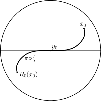
The problem of global integrability is in general more subtle than local integrability. As a matter of fact, in Example 10.4.1 we construct an example of a locally integrable immersion G:(−T,T)→𝔾2G:(-T,T)\to\mathbb{G}_{2}, defined for some T∈ℝ+T\in{\mathbb{R}}^{+}, that is not globally integrable. By taking a cylinder on this curve, one easily sees that the same phenomenon occurs in any dimension. We stress that in our example M=(−T,T)M=(-T,T) (or the product (−T,T)×ℝn−1(-T,T)\times{\mathbb{R}}^{n-1} for n>2n>2) is simply connected: the key point in our example is that one can find globally defined maps ζ:M→T1​ℍn+1\zeta:M\to T^{1}\mathbb{H}^{n+1} such that G=p∘ζG=\mathrm{p}\circ\zeta, but no such ζ\zeta projects to an immersion in ℍn+1\mathbb{H}^{n+1}.

Nevertheless, we show that this issue does not occur for Riemannian immersions GG. In this case any immersion σ\sigma whose Gauss map is GG (if it exists) necessarily has small principal curvatures. We will always restrict to this setting hereafter. In summary, we have the following characterization of global integrability for MM simply connected.

Theorem 10.4.2.

Let MnM^{n} be a simply connected manifold and G:M→𝔾n+1G\colon M\to\mathbb{G}_{n+1} be a Riemannian immersion. Then GG is globally integrable if and only if it is Lagrangian.

We give a characterization of global integrability for π1​(M)≠{1}\pi_{1}(M)\neq\{1\} in Corollary 10.5.6, which is a direct consequence of our first characterization of ρ\rho-integrability (Theorem 10.5.5). Anyway, we remark that if a Riemannian and Lagrangian immersion G:M→𝔾n+1G\colon M\to\mathbb{G}_{n+1} is also complete (i.e. has complete first fundamental form), then MM is necessarily simply connected:

Theorem 10.4.3.

Let MnM^{n} be a manifold. If G:M→𝔾n+1G\colon M\to\mathbb{G}_{n+1} is a complete Riemannian and Lagrangian immersion, then MM is diffeomorphic to ℝn{\mathbb{R}}^{n} and GG is the Gauss map of a proper embedding σ:M→ℍn+1\sigma:M\to\mathbb{H}^{n+1}.

In Theorem 10.4.3 the conclusion that G=GσG=G_{\sigma} for σ\sigma a proper embedding follows from the fact that σ\sigma is complete, which is an easy consequence of Equation (9.4) relating the first fundamental forms of σ\sigma and GσG_{\sigma}, and the non-trivial fact that complete immersions in ℍn+1\mathbb{H}^{n+1} with small principal curvatures are proper embeddings (Proposition 9.3.15).

Equivariant integrability

Let us first observe that the problem of ρ\rho-integrability presents some additional difficulties than global integrability. Assume G:M~→𝔾n+1G\colon\widetilde{M}\to\mathbb{G}_{n+1} is a Lagrangian, Riemannian and ρ\rho-equivariant immersion for some representation ρ:π1​(Mn)→Isom⁡(ℍn+1)\rho\colon\pi_{1}(M^{n})\to\mathrm{Isom}(\mathbb{H}^{n+1}). Then, by Theorem 10.4.2, there exists σ:M~→ℍn+1\sigma\colon\widetilde{M}\to\mathbb{H}^{n+1} with Gauss map GG, but the main issue is that such a σ\sigma will not be ρ\rho-equivariant in general, as one can see in Examples 10.5.1 and 10.5.2.

Nevertheless, ρ\rho-integrability of Riemannian immersions into 𝔾n+1\mathbb{G}_{n+1} can still be characterized in terms of their extrinsic geometry. Let H¯\overline{\mathrm{H}} be the mean curvature vector of GG, defined as the trace of the second fundamental form, and let Ω\Omega be the symplectic form of 𝔾n+1\mathbb{G}_{n+1}. Since GG is ρ\rho-equivariant, the 11-form G∗​(Ω​(H¯,⋅))G^{*}(\Omega(\overline{\mathrm{H}},\cdot)) on M~\widetilde{M} is invariant under the action of π1​(M)\pi_{1}(M), so it descends to a 11-form on MM. One can prove that such 11-form on MM is closed (Corollary 10.5.9): we will denote with μG\mu_{G} its cohomology class in Hd​R1​(M,ℝ)H^{1}_{dR}(M,{\mathbb{R}}) and we will call it the Maslov class of GG, in accordance with some related interpretations of the Maslov class in other geometric contexts (see, among others, [Mor81, Oh94, Ars00, Smo02]). The Maslov class encodes the existence of equivariantly integrating immersions, in the sense stated in the following theorem.

Theorem 10.5.5.

Let MnM^{n} be an orientable manifold, ρ:π1​(M)→Isom⁡(ℍn+1)\rho\colon\pi_{1}(M)\to\mathrm{Isom}(\mathbb{H}^{n+1}) be a representation and G:M~→𝔾n+1G\colon\widetilde{M}\to\mathbb{G}_{n+1} be a ρ\rho-equivariant Riemannian and Lagrangian immersion. Then GG is ρ\rho-integrable if and only if the Maslov class μG\mu_{G} vanishes.

Applying Theorem 10.5.5 to a trivial representation, we immediately obtain a characterization of global integrability for Riemannian immersions, thus extending Theorem 10.4.2 to the case π1​(M)≠{1}\pi_{1}(M)\neq\{1\}.

Corollary 10.5.6.

Let MnM^{n} be an orientable manifold and G:M→𝔾n+1G\colon M\to\mathbb{G}_{n+1} be a Riemannian and Lagrangian immersion. Then GG is globally integrable if and only if its Maslov class μG\mu_{G} vanishes.

1.3.2 Nearly-Fuchsian representations

Let us now focus on the case for which MM is a closed oriented manifold. Although our results apply to any dimension, we borrow the terminology from the three-dimensional case (see [HW13]) and say that a representation ρ:π1​(M)→Isom⁡(ℍn+1)\rho\colon\pi_{1}(M)\to\mathrm{Isom}(\mathbb{H}^{n+1}) is nearly-Fuchsian if there exists a ρ\rho-equivariant immersion σ:M~→ℍn+1\sigma\colon\widetilde{M}\to\mathbb{H}^{n+1} with small principal curvatures. We show (Proposition 9.4.2) that the action of a nearly-Fuchsian representation on ℍn+1\mathbb{H}^{n+1} is free, properly discontinuously and convex cocompact; the quotient of ℍn+1\mathbb{H}^{n+1} by ρ​(π1​(M))\rho(\pi_{1}(M)) is called nearly-Fuchsian manifold.

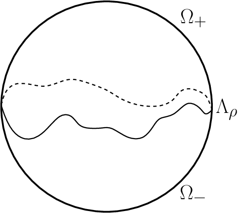
Moreover, the action of ρ​(π1​(M))\rho(\pi_{1}(M)) extends to a free and properly discontinuous action on the complement of a topological (n−1)(n-1)-sphere Λρ\Lambda_{\rho} (the limit set of ρ\rho) in the visual boundary ∂ℍn+1\partial\mathbb{H}^{n+1}. Such complement is the disjoint union of two topological nn-discs which we denote by Ω+\Omega_{+} and Ω−\Omega_{-}. It follows that there exists a maximal open region of 𝔾n+1\mathbb{G}_{n+1} over which a nearly-Fuchsian representation ρ\rho acts freely and properly discontinuously. This region is defined as the subset of 𝔾n+1\mathbb{G}_{n+1} consisting of oriented geodesics having either final endpoint in Ω+\Omega_{+} or initial endpoint in Ω−\Omega_{-}. The quotient of this open region via the action of ρ\rho, that we denote with 𝒢ρ\mathcal{G}_{\rho}, inherits a para-Kähler structure.

Let us first state a uniqueness result concerning nearly-Fuchsian representations. A consequence of Theorem 10.5.5 and the definition of Maslov class is that if GG is a ρ\rho-equivariant, Riemannian and Lagrangian immersion which is furthermore minimal, i.e. with H¯=0\overline{\mathrm{H}}=0, then it is ρ\rho-integrable. Together with an application of a maximum principle in the corresponding nearly-Fuchsian manifold, we prove:

Corollary 10.6.3.

Given a closed orientable manifold MnM^{n} and a representation ρ:π1​(M)→Isom⁡(ℍn+1)\rho:\pi_{1}(M)\to\mathrm{Isom}(\mathbb{H}^{n+1}), there exists at most one ρ\rho-equivariant Riemannian minimal Lagrangian immersion G:M~→𝔾n+1G:\widetilde{M}\to\mathbb{G}_{n+1} up to reparametrization. If such a GG exists, then ρ\rho is nearly-Fuchsian and GG induces a minimal Lagrangian embedding of MM in 𝒢ρ\mathcal{G}_{\rho}.

In fact, for any ρ\rho-equivariant immersion σ:M~→ℍn+1\sigma:\widetilde{M}\to\mathbb{H}^{n+1} with small principal curvatures, the hyperbolic Gauss maps Gσ±G_{\sigma}^{\pm} are equivariant diffeomorphisms between M~\widetilde{M} and Ω±\Omega_{\pm}. Hence up to changing the orientation of MM, which corresponds to swapping the two factors ∂ℍn+1\partial\mathbb{H}^{n+1} in the identification 𝔾n+1≅∂ℍn+1×∂ℍn+1∖Δ\mathbb{G}_{n+1}\cong\partial\mathbb{H}^{n+1}\times\partial\mathbb{H}^{n+1}\setminus\Delta, the Gauss map of σ\sigma takes values in the maximal open region defined above, and induces an embedding of MM in 𝒢ρ\mathcal{G}_{\rho}.

This observations permits to deal (in the cocompact case) with embeddings in 𝒢ρ\mathcal{G}_{\rho} instead of ρ\rho-equivariant embeddings in 𝔾n+1\mathbb{G}_{n+1}. In analogy with the definition of ρ\rho-integrability defined above, we will say that a nn-dimensional submanifold ℒ⊂𝒢ρ\mathcal{L}\subset\mathcal{G}_{\rho} is ρ\rho-integrable if it is the image in the quotient of a ρ\rho-integrable embedding in 𝔾n+1\mathbb{G}_{n+1}. Clearly such ℒ\mathcal{L} is necessarily Lagrangian by Theorem 10.3.4. We are now ready to state our second characterization result for ρ\rho-integrability.

Theorem 11.1.4.

Let MM be a closed orientable nn-manifold, ρ:π1​(M)→Isom⁡(ℍn+1)\rho:\pi_{1}(M)\to\mathrm{Isom}(\mathbb{H}^{n+1}) be a nearly-Fuchsian representation and ℒ⊂𝒢ρ\mathcal{L}\subset\mathcal{G}_{\rho} be a Riemannian ρ\rho-integrable submanifold. Then a Riemannian submanifold ℒ′\mathcal{L}^{\prime} is ρ\rho-integrable if and only if there exists Φ∈Hamc​(𝒢ρ,Ω)\Phi\in\mathrm{Ham}_{c}(\mathcal{G}_{\rho},\Omega) such that Φ⁡(ℒ)=ℒ′\Phi(\mathcal{L})=\mathcal{L}^{\prime}.

In Theorem 11.1.4 we denoted by Hamc​(𝒢ρ,Ω)\mathrm{Ham}_{c}(\mathcal{G}_{\rho},\Omega) the group of compactly-supported Hamiltonian symplectomorphisms of 𝒢ρ\mathcal{G}_{\rho} with respect to its symplectic form Ω\Omega. (See Definition 11.1.2). The proof of Theorem 11.1.4 in fact shows that if ℒ\mathcal{L} is ρ\rho-integrable and ℒ′=Φ⁡(ℒ)\mathcal{L}^{\prime}=\Phi(\mathcal{L}) for Φ∈Hamc​(𝒢ρ,Ω)\Phi\in\mathrm{Ham}_{c}(\mathcal{G}_{\rho},\Omega), then ℒ′\mathcal{L}^{\prime} is integrable as well, even without the hypothesis that ℒ\mathcal{L} and ℒ′\mathcal{L}^{\prime} are Riemannian submanifolds.

If ρ\rho admits an equivariant Riemannian minimal Lagrangian immersion, then Theorem 11.1.4 can be restated by saying that a Riemannian and Lagrangian submanifold ℒ′\mathcal{L}^{\prime} is ρ\rho-integrable if and only if it is in the Hamc​(𝒢ρ,Ω)\mathrm{Ham}_{c}(\mathcal{G}_{\rho},\Omega)-orbit of the minimal Lagrangian submanifold ℒ⊂𝒢ρ\mathcal{L}\subset\mathcal{G}_{\rho}, which is unique by Theorem 10.6.3.

1.3.3 Relation with geometric flows

Finally, in Section 11.4 we apply these methods to study the relation between evolutions by geometric flows in ℍn+1\mathbb{H}^{n+1} and in 𝔾n+1\mathbb{G}_{n+1}. More precisely, suppose that σ∙:M×(−ϵ,ϵ)→ℍn+1\sigma_{\bullet}:M\times(-\epsilon,\epsilon)\to\mathbb{H}^{n+1} is a smoothly varying family of Riemannian immersions that satisfy:

dd​t​σt=ft​νt\frac{d}{dt}\sigma_{t}=f_{t}\nu_{t}

where νt\nu_{t} is the normal vector of σt\sigma_{t} and f∙:M×(−ϵ,ϵ)→ℝf_{\bullet}:M\times(-\epsilon,\epsilon)\to{\mathbb{R}} is a smooth function. Then the variation of the Gauss map GtG_{t} of σt\sigma_{t} is given, up to a tangential term, by the normal term −𝕁⁡(d​Gt​(∇¯​ftt))-\mathbbm{J}(dG_{t}({\overline{\nabla}}{}^{t}f_{t})), where ∇¯​ftt{\overline{\nabla}}{}^{t}f_{t} denotes the gradient with respect to the first fundamental form of GtG_{t}, that is, the Riemannian metric Gt∗​𝕘G_{t}^{*}{\mathbbm{g}}.

Let us consider the special case of the flow defined by ft:=κσtf_{t}:=\kappa_{\sigma_{t}}, where κσt\kappa_{\sigma_{t}} is defined as the sum of the hyperbolic arctangent of the principal curvatures of σt\sigma_{t} (see Equation (9.9)). The study of the associated flow has been suggested in dimension three in [And02], by analogy with a similar flow on surfaces in the three-sphere. Combining the aforementioned result of Section 11.4 with Proposition 10.5.7, we obtain that such flow in ℍn+1\mathbb{H}^{n+1} induces the Lagrangian mean curvature flow in 𝔾n+1\mathbb{G}_{n+1} up to tangential diffeomorphisms. A similar result has been obtained in Anti-de Sitter space (in dimension three) in [Smo13].

Part I The ambient spaces

Chapter 2 Pseudo-Riemannian space forms

2.1 Pseudo-Riemannian metrics

We recall some very basic concepts in differential geometry in order to fix the notation. The reader may refer to [ONe83, KN96a] as good textbooks on these topics.

Let M=MnM=M^{n} be a smooth manifold of dimension nn. Throughout all the paper, we will assume MM to be connected.

A pseudo-Riemannian metric gg on MM is a smooth section of the bundle S​y​m2​(T​M)Sym^{2}(TM) such that the bilinear form gx:Tx​M×Tx​M→ℝg_{x}\colon T_{x}M\times T_{x}M\to{\mathbb{R}} is non-degenerate. By connectedness of MM, the bilinear form gxg_{x} has constant signature for all x∈Mx\in M.

A Riemannian metric gg on MM is a pseudo-Riemannian metric such that gxg_{x} is positive-definite for all x∈Mx\in M. We say that (M,g)(M,g) is a (pseudo-)Riemannian manifold if gg is (pseudo-)Riemannian. As a matter of notation, we will often denote pseudo-Riemannian manifolds with MM instead of (M,g)(M,g).

An affine connection ∇\nabla on a manifold MM is a linear map

∇:Γ⁡(T​M)\displaystyle\nabla\colon\Gamma(TM) →E​n​d​(T​M)\displaystyle\to End(TM)
X\displaystyle X ↦∇X(:Y↦∇YX).\displaystyle\mapsto\nabla X(\colon Y\mapsto\nabla_{Y}X).

such that, for all X,Y∈Γ⁡(T​M)X,Y\in\Gamma(TM) and f:M→ℝf\colon M\to{\mathbb{R}},

∇(fY)=df⊗Y+f∇Y.\nabla(fY)=df\otimes Y+f\nabla Y.

A pseudo-Riemannian metric gg induces canonically an affine connection, called Levi-Civita connection of gg, defined as the unique affine connection with the following properties:

  • •

    ∇\nabla is compatible with the metric, i.e. for all X,Y∈Γ⁡(T​M)X,Y\in\Gamma(TM), d⁡(g⁡(X,Y))=g⁡(∇X,Y)+g⁡(X,∇Y)d\big(g(X,Y)\big)=g(\nabla X,Y)+g(X,\nabla Y);

  • •

    ∇\nabla is torsion-free, i.e. for all X,Y∈Γ⁡(T​M)X,Y\in\Gamma(TM), ∇XY−∇YX=[X,Y]\nabla_{X}Y-\nabla_{Y}X=[X,Y].

A connection ∇\nabla comes with a notion of parallel transport, geodesics and exponential map. Since the exponential map at any point of MM is a local diffeomorphism, for every point xx of MM there exists a starred neighborhood UxU_{x}, namely UxU_{x} is such that any of its points can be connected to xx through a geodesic segment.

Lemma 2.1.1.

Let f1,f2:(M,g)→(N,h)f_{1},f_{2}\colon(M,g)\to(N,h) be two isometries between pseudo-Riemannian manifolds (with MM connected) such that, for some point x∈𝕄x\in\mathbb{M}, f1​(x)=f2​(x)f_{1}(x)=f_{2}(x) and dx​f1=dx​f2:Tx​M→Tf1​(x)​Nd_{x}f_{1}=d_{x}f_{2}\colon T_{x}M\to T_{f_{1}(x)}N. Then f1≡f2f_{1}\equiv f_{2}.

Proof.

Being f,gf,g isometries, one has that

f∘e​x​pxM=e​x​pf⁡(x)N∘dx​f=e​x​pg⁡(x)N∘dx​g=g∘e​x​pxM,f\circ exp_{x}^{M}=exp_{f(x)}^{N}\circ d_{x}f=exp_{g(x)}^{N}\circ d_{x}g=g\circ exp_{x}^{M}\ ,

so ff and gg coincide on any open neighbourhood of xx whose elements can be linked to xx by a geodesic segment. For all y∈My\in M, one can take a connected compact subset of MM containg both xx and yy (e.g. a curve) and cover it by a finite amount of starred open subsets of MM. By iteration of the argument above and by standard deductions, one gets that ff and gg coincide on yy. ∎

We say that a pseudo-Riemannian manifold is complete if its Levi-Civita connection is geodesically complete, namely if geodesics can be extended indefinitely. If the metric is not Riemannian, it is generally false that any two points on the manifold can be connected by a geodesic segment.

An affine connection ∇\nabla defines a (1,3)(1,3)-type curvature tensor R∈Γ⁡(T∗​M⊗T∗​M⊗T∗​M⊗T​M)R\in\Gamma(T^{*}M\otimes T^{*}M\otimes T^{*}M\otimes TM) as

R⁡(X,Y)​Z:=∇X∇Y​Z−∇Y∇X​Z−∇[X,Y]Z.R(X,Y)Z:=\nabla_{X}\nabla_{Y}Z-\nabla_{Y}\nabla_{X}Z-\nabla_{[X,Y]}Z.

If (M,g)(M,g) is a pseudo-Riemannian manifold, one also has a (0,4)(0,4)-type curvature tensor, that we will still denote with RR, defined as

R⁡(X,Y,Z,T):=−g⁡(R⁡(X,Y)​Z,T).R(X,Y,Z,T):=-g(R(X,Y)Z,T).

The (0,4)(0,4)-type curvature tensor has several symmetries, generated by the equations

R⁡(X,Y,Z,T)=−R⁡(Y,X,Z,T)R⁡(X,Y,Z,T)=R⁡(Z,T,X,Y)R⁡(X,Y,Z,T)+R⁡(Y,Z,X,T)+R⁡(Z,X,Y,T)=0.\begin{split}&R(X,Y,Z,T)=-R(Y,X,Z,T)\\ &R(X,Y,Z,T)=R(Z,T,X,Y)\\ &R(X,Y,Z,T)+R(Y,Z,X,T)+R(Z,X,Y,T)=0.\end{split} (2.1)

For all x∈Mx\in M, given a 22-dimensional vector subspace 𝒱<Tx​M\mathcal{V}<T_{x}M such that gx|𝒱{g_{x}|}_{\mathcal{V}} is non degenerate, the sectional curvature of 𝒱\mathcal{V} is defined as

K⁡(𝒱)=R⁡(X,Y,X,Y)g⁡(X,X)​g​(Y,Y)−(g⁡(X,Y))2K(\mathcal{V})=\frac{R(X,Y,X,Y)}{g(X,X)g(Y,Y)-(g(X,Y))^{2}}

with 𝒱=S​p​a​nℝ​(X,Y)\mathcal{V}=Span_{\mathbb{R}}(X,Y). The multilinearity of RR and gg and the symmetries of RR ensure that the definition does not depend on the choice of the generators X,YX,Y for 𝒱\mathcal{V}.

2.2 Pseudo-Riemannian space forms: uniqueness

We say that the pseudo-Riemannian manifold (M,g)(M,g) has constant sectional curvature k∈ℝk\in{\mathbb{R}} if, for all x∈Mx\in M and for all gg-non-degenerate 2-dimensional vector subspace 𝒱<Tx​M\mathcal{V}<T_{x}M, K⁡(𝒱)=kK(\mathcal{V})=k.

We will say that a pseudo-Riemannian manifold (M,g)(M,g) is a space form if it is simply connected, complete and with constant sectional curvature.

Theorem 2.2.1.

For all n,m∈ℤ≥0n,m\in{\mathds{Z}}_{\geq 0}, with n≥2n\geq 2 and m≤nm\leq n, and k∈ℝk\in{\mathbb{R}}, there exists a unique pseudo-Riemannian space form of dimension nn, signature (m,n−m)(m,n-m) and constant curvature kk, up to isometries.

Despite Theorem 2.2.1 is a classical result in Differential Geometry, it will be convenient to recall one way to prove the uniqueness part of the statement because we will use the same idea for a main proof later on.

Step 11: The Cartan-Ambrose-Hicks Theorem for affine manifolds.

Let MM and NN be two smooth manifolds of the same dimension nn, let ∇M\nabla^{M} and ∇N\nabla^{N} be two linear connections on T​MTM and on T​NTN respectively. The pair (M,∇M)(M,\nabla^{M}) (and (N,∇N)(N,\nabla^{N})) is often called an affine manifold. Assume that ∇M\nabla^{M} and ∇N\nabla^{N} are complete and that MM is simply connected.

For convenience, assume both ∇M\nabla^{M} and ∇N\nabla^{N} are torsion-free. Fix x0∈Mx_{0}\in M and y0∈Ny_{0}\in N and assume L:Tx0​M→Ty0​NL\colon T_{x_{0}}M\to T_{y_{0}}N is a linear isomorphism. For all X∈Tx0​MX\in T_{x_{0}}M and for any given τ>0\tau>0, consider the geodesic γ⁡(t)=e​x​pM​(t​X)\gamma(t)=exp^{M}(tX) with t∈[0,τ]t\in[0,\tau] and the geodesic curve γL​(t)=e​x​pN​(t​L​(X))\gamma_{L}(t)=exp^{N}(tL(X)) with t∈[0,τ]t\in[0,\tau]: the composition of LL with the parallel transports via the geodesics γ\gamma and γL\gamma_{L} induces a linear isomorphism

Lγ:Tγ⁡(τ)​M→TγL​(τ)​N.L_{\gamma}\colon T_{\gamma(\tau)}M\to T_{\gamma_{L}(\tau)}N.

By iterating this argument, one gets that any piecewise geodesic curve γ:[0,τ]→M\gamma\colon[0,\tau]\to M with starting point x0x_{0} induces a piecewise geodesic curve γL:[0,τ]→N\gamma_{L}\colon[0,\tau]\to N with starting point y0y_{0} and the composition of LL with the parallel transports defines once again a linear isomorphism Lγ:Tγ⁡(τ)​M→TγL​(τ)​NL_{\gamma}\colon T_{\gamma(\tau)}M\to T_{\gamma_{L}(\tau)}N.

Recall that, being MM (and NN) connected, any two of its points can be linked by a piecewise geodesic curve.

Theorem 2.2.2 (Ambrose-Cartan-Hicks Theorem).

Under the notations and the assumptions above, if for all piecewise geodesic curve γ:[0,τ]→M\gamma\colon[0,\tau]\to M with γ⁡(0)=x0\gamma(0)=x_{0} the corresponding isomorphism Lγ:Tγ⁡(τ)​M→Tγϕ​(τ)​NL_{\gamma}\colon T_{\gamma(\tau)}M\to T_{\gamma_{\phi}(\tau)}N preserves the curvature tenors, namely

Lγ​(RM​(X1,X2)​X3)=RN​(Lγ​(X1),Lγ​(X2))​(Lγ​(X3))L_{\gamma}(R^{M}(X_{1},X_{2})X_{3})=R^{N}(L_{\gamma}(X_{1}),L_{\gamma}(X_{2}))(L_{\gamma}(X_{3})) (2.2)

for all X1,X2,X3∈Tγ⁡(T)​MX_{1},X_{2},X_{3}\in T_{\gamma(T)}M, then there exists a unique covering map f:M→Nf\colon M\to N such that:

  • •

    ff is affine, i.e. f∗​∇N=∇Mf^{*}\nabla^{N}=\nabla^{M};

  • •

    f⁡(x0)=y0f(x_{0})=y_{0} and dx0​f=Ld_{x_{0}}f=L;

  • •

    for all piecewise geodesic curve γ:[0,τ]→M\gamma\colon[0,\tau]\to M starting at x0x_{0}, f⁡(γ⁡(τ))=γL​(τ)f(\gamma(\tau))=\gamma_{L}(\tau) with dγ⁡(τ)​f=Lγd_{\gamma(\tau)}f=L_{\gamma}.

For a proof of Theorem 2.2.2 see [PT05].

Step 22: The curvature tensor of manifolds with constant sectional curvature.

Proposition 2.2.3.

Let MM be a manifold and let R,R′∈Γ(T∗M4⊗)R,R^{\prime}\in\Gamma(T^{*}M^{4\otimes}) be two (0,4)(0,4)-type tensors both satisfying Equations (2.1). If

R⁡(X,Y,X,Y)=R′​(X,Y,X,Y)R(X,Y,X,Y)=R^{\prime}(X,Y,X,Y)

for all X,Y∈Γ⁡(T​M)X,Y\in\Gamma(TM), then R≡R′R\equiv R^{\prime}.

Proof.

Observe that the tensor R−R′R-R^{\prime} satisfies Equations (2.1), being the equations linear, and that it is such that (R−R′)​(X,Y,X,Y)=0(R-R^{\prime})(X,Y,X,Y)=0 for all X,Y∈Γ⁡(T​M)X,Y\in\Gamma(TM). For all W,X,Y,Z∈Γ⁡(T​M)W,X,Y,Z\in\Gamma(TM), we have

(R−R′)​(X,Y+Z,X,Y+Z)=0⟹(R−R′)​(X,Y,X,Z)=0;\displaystyle(R-R^{\prime})(X,Y+Z,X,Y+Z)=0\Longrightarrow(R-R^{\prime})(X,Y,X,Z)=0;
(R−R′)​(X+W,Y,X+W,Z)=0⟹(R−R′)​(X,Y,W,Z)=(R−q)​(Y,W,X,Z);\displaystyle(R-R^{\prime})(X+W,Y,X+W,Z)=0\Longrightarrow(R-R^{\prime})(X,Y,W,Z)=(R-q)(Y,W,X,Z);
(R−R′)​(X,Y,W,Z)+(R−R′)​(W,X,Y,Z)+(R−R′)​(Y,W,X,Z)=0⟹\displaystyle(R-R^{\prime})(X,Y,W,Z)+(R-R^{\prime})(W,X,Y,Z)+(R-R^{\prime})(Y,W,X,Z)=0\Longrightarrow
⟹2​(R−R′)​(X,Y,W,Z)=(R−R′)​(X,W,Y,Z);\displaystyle\qquad\qquad\Longrightarrow 2(R-R^{\prime})(X,Y,W,Z)=(R-R^{\prime})(X,W,Y,Z);

then 4​(R−R′)​(X,Y,W,Z)=2​(R−R′)​(X,W,Y,Z)=(R−R′)​(X,Y,W,Z)4(R-R^{\prime})(X,Y,W,Z)=2(R-R^{\prime})(X,W,Y,Z)=(R-R^{\prime})(X,Y,W,Z), hence R−R′≡0R-R^{\prime}\equiv 0. ∎

Corollary 2.2.4.

If (M,g)(M,g) is a pseudo-Riemannian manifold of constant sectional curvature k∈ℝk\in{\mathbb{R}}, then, for any X,Y,Z,W∈Γ⁡(T​𝕄)X,Y,Z,W\in\Gamma(T\mathbb{M}),

R⁡(X,Y,Z,W)=k⁡(g⁡(X,Z)​g​(Y,W)−g⁡(Y,Z)​g​(X,W)),R(X,Y,Z,W)=k(g(X,Z)g(Y,W)-g(Y,Z)g(X,W)),

or equivalently

R⁡(X,Y)​Z=−k⁡(g⁡(X,Z)​Y−g⁡(Y,Z)​X).R(X,Y)Z=-k(g(X,Z)Y-g(Y,Z)X).

In particular, R⁡(X,Y)​Z∈S​p​a​n​(X,Y)R(X,Y)Z\in Span(X,Y).

Proof.

The tensor R′​(X,Y,Z,W)=k⁡(g⁡(X,Z)​g​(Y,W)−g⁡(Y,Z)​g​(X,W))R^{\prime}(X,Y,Z,W)=k(g(X,Z)g(Y,W)-g(Y,Z)g(X,W)) satisfies Equations (2.1) and is such that R′​(X,Y,X,Y)=R⁡(X,Y,X,Y)R^{\prime}(X,Y,X,Y)=R(X,Y,X,Y) for all X,Y∈Γ⁡(T​M)X,Y\in\Gamma(TM). ∎

Step 33: Conclusion.

Proof of Theorem 2.2.1.

Let (M,g)(M,g) and (N,h)(N,h) be two simply connected, complete pseudo-Riemannian manifolds of dimension nn, signature (m,n−m)(m,n-m) and with constant sectional curvature kk. Denote with ∇M\nabla^{M} and ∇N\nabla^{N} respectively their Levi-Civita connections. Fix x∈Mx\in M and y∈Ny\in N.

By standard linear algebra, there exists a linear isometry L:(Tx​M,gx)→(Ty​N,gy)L\colon(T_{x}M,g_{x})\to(T_{y}N,g_{y}) because Tx​MT_{x}M and Ty​NT_{y}N have the same dimension, and gxg_{x} and hyh_{y} have the same signature. With notations as in Step 1, let γ:[0,τ]→M\gamma\colon[0,\tau]\to M be a geodesic with γ⁡(0)=x\gamma(0)=x and let γL:[0,τ]→N\gamma_{L}\colon[0,\tau]\to N such that γ˙L​(0)=L⁡(γ˙​(0))\dot{\gamma}_{L}(0)=L(\dot{\gamma}(0)). Since parallel transport along γ\gamma defines an isometry between the tangent spaces Tγ⁡(0)​M→Tγ⁡(τ)​NT_{\gamma(0)}M\to T_{\gamma(\tau)}N, and likewise for γL\gamma_{L}, the induced map

Lγ:(Tγ⁡(τ)​M,g)→(TγL​(τ)​N,h)L_{\gamma}\colon(T_{\gamma(\tau)}M,g)\to(T_{\gamma_{L}(\tau)}N,h)

is a linear isometry. By iteration, the same holds for LγL_{\gamma} when γ\gamma is a piecewise geodesic curve starting at xx.

By Corollary 2.2.4 applied to both MM and NN and by the fact that LγL_{\gamma} is an isometry, for all X,Y,Z∈TγL​(τ)​MX,Y,Z\in T_{\gamma_{L}(\tau)}M one gets that

Lγ​(RM​(X,Y)​Z)\displaystyle L_{\gamma}(R^{M}(X,Y)Z) =−k​g​(X,Z)​Lγ​(Y)+k​g​(Y,Z)​Lγ​(X)=\displaystyle=-k\ g(X,Z)L_{\gamma}(Y)+k\ g(Y,Z)L_{\gamma}(X)=
=−k​h​(Lγ​(X),Lγ​(Z))​Lγ​(Y)+k​h​(Lγ​(Y),Lγ​(Z))​Lγ​(X)=\displaystyle=-k\ h(L_{\gamma}(X),L_{\gamma}(Z))L_{\gamma}(Y)+k\ h(L_{\gamma}(Y),L_{\gamma}(Z))L_{\gamma}(X)=
=RN​(Lγ​(X),Lγ​(Y))​(Lγ​(Z)).\displaystyle=R^{N}(L_{\gamma}(X),L_{\gamma}(Y))(L_{\gamma}(Z)).

By Theorem 2.2.2, there exists a covering map f:M→Nf\colon M\to N such that for every piecewise geodesic curve γ:[0,τ]→M\gamma\colon[0,\tau]\to M starting at xx, dγ⁡(τ)​f=Lγd_{\gamma(\tau)}f=L_{\gamma}, hence ff is a local isometry. Since MM and NN are both simply connected, ff is an isometry. ∎

Remark 2.2.5.

The proof of 2.2.1 leads to another observation: if (M,g)(M,g) is a pseudo-Riemannian space form, then, for any given x∈Mx\in M and any given linear isometry L:(Tx​M,gx)→(Tx​M,gx)L\colon(T_{x}M,g_{x})\to(T_{x}M,g_{x}), there exists an isometry f:(M,g)→(M,g)f\colon(M,g)\to(M,g) such that f⁡(x)=xf(x)=x and dx​f=Ld_{x}f=L.

We will denote with 𝔽km1,m2=(𝔽km1,m2,⟨⋅,⋅⟩)\mathbb{F}_{k}^{m_{1},m_{2}}=(\mathbb{F}_{k}^{m_{1},m_{2}},\langle\cdot,\cdot\rangle) the pseudo-Riemannian space form of dimension m1+m2≥2m_{1}+m_{2}\geq 2, signature (m1,m2)(m_{1},m_{2}) and constant sectional curvature k∈ℝk\in{\mathbb{R}}.

We will discuss existence of pseudo-Riemannian space forms in Section 2.4, after recalling the Gauss-Codazzi Theorem. The reader might find quite unusual to work with space forms before proving they exist, but hopefully the reason behind this choice will be clear later on.

2.3 Immersions of hypersurfaces into pseudo-Riemannian space forms

There exists a general theory of immersions of manifolds into pseudo-Riemannian space forms. In the following we stick to the theory of hypersurfaces, where the theory has a more simple description. The reader might refer for instance to [LTV10] which treats the topic in the general setting of immersions of any codimension into products of space forms.

The setting is very classical and in the following we will skip the main proofs. Nevertheless, in Chapter 6, we will handle a similar formalism to study immersions of smooth manifolds of dimension nn into (n+1)(n+1)-dimensional holomorphic Riemannian space forms and we will provide all the major proofs: mutatis mutandis, proofs in the pseudo-Riemannian setting work in the same fashion with some more attention to signatures but with generally fewer technical precautions.

Let M=MnM=M^{n} be an orientable nn-dimensional manifold, let m1,m2m_{1},m_{2} be two integers with m1+m2=n+1m_{1}+m_{2}=n+1, and denote 𝔽=(𝔽km1,m2,⟨⋅,⋅⟩)\mathbb{F}=(\mathbb{F}_{k}^{m_{1},m_{2}},\langle\cdot,\cdot\rangle). Equip both 𝔽\mathbb{F} and MM with an orientation.

We say that an immersion σ:M→𝔽\sigma\colon M\to\mathbb{F} is admissible if the pull-back metric I=σ∗​⟨⋅,⋅⟩\mathrm{I}=\sigma^{*}\langle\cdot,\cdot\rangle is a (non-degenerate) pseudo-Riemannian metric on MM. The pull-back metric I\mathrm{I} falls within one of the following two cases:

  • Case (aa):

    I\mathrm{I} has signature (m1−1,m2)(m_{1}-1,m_{2});

  • Case (bb):

    I\mathrm{I} has signature (m1,m2−1)(m_{1},m_{2}-1).

The map d​σd\sigma induces a canonical bundle inclusion of T​M<σ∗​(T​𝔽)TM<\sigma^{*}(T\mathbb{F}). In order to relax the notation, we denote with ⟨⋅,⋅⟩\langle\cdot,\cdot\rangle also the pull-back metric on σ∗​(T​𝔽)\sigma^{*}(T\mathbb{F}). By construction, ⟨⋅,⋅⟩|TM=I\langle\cdot,\cdot\rangle_{|TM}=\mathrm{I}.

There exists a unique section ν∈Γ⁡(σ∗​(T​𝔽))\nu\in\Gamma(\sigma^{*}(T\mathbb{F})) such that ⟨ν,ν⟩=1\langle\nu,\nu\rangle=1 if in case (a)(a) and such that ⟨ν,ν⟩=−1\langle\nu,\nu\rangle=-1 if in case (b)(b) and so that (d​σ​(e1),…,d​σ​(en),d​σ​(ν))(d\sigma(e_{1}),\dots,d\sigma(e_{n}),d\sigma(\nu)) is an oriented frame for 𝔽\mathbb{F} whenever (e1,…,en)(e_{1},\dots,e_{n}) is an oriented frame for MM. Such ν\nu is a (global) normal vector field.

Denote with ∇\nabla the Levi-Civita connection on T​MTM with respect to I\mathrm{I} and with ∇¯\overline{\nabla} the Levi-Civita connection on σ∗​(T​𝔽)\sigma^{*}(T\mathbb{F}) with respect to ⟨⋅,⋅⟩\langle\cdot,\cdot\rangle, namely the pull-back of the Levi-Civita connection of ⟨⋅,⋅⟩\langle\cdot,\cdot\rangle on T​𝔽T\mathbb{F}. One has that, for all X,Y∈Γ⁡(T​M)X,Y\in\Gamma(TM),

∇¯X​Y=∇XY+II⁡(X,Y)​ν,\overline{\nabla}_{X}Y=\nabla_{X}Y+\mathrm{I}\hskip-1.13791pt\mathrm{I}(X,Y)\nu\ ,

where II\mathrm{I}\hskip-1.13791pt\mathrm{I} is called second fundamental form of σ\sigma and is a symmetric (0,2)(0,2)-tensor on T​MTM.

By raising an index and changing a sign, one can define the shape operator BB for σ\sigma as the (1,1)(1,1)-tensor on T​MTM defined by

I⁡(B⁡(X),Y):=II⁡(X,Y).\mathrm{I}(B(X),Y):=\mathrm{I}\hskip-1.13791pt\mathrm{I}(X,Y).

Since II\mathrm{I}\hskip-1.13791pt\mathrm{I} is symmetric, BB is I\mathrm{I}-self adjoint.

Define the exterior covariant derivative of a (1,1)(1,1)-tensor β\beta with respect to the connection ∇\nabla as the skew-symmetric (1,2)(1,2)-tensor defined by

d∇​β​(X,Y)=∇X(β⁡(Y))−∇Y(β⁡(X))−β⁡([X,Y]).d^{\nabla}\beta(X,Y)=\nabla_{X}(\beta(Y))-\nabla_{Y}(\beta(X))-\beta([X,Y]).

The following result is known as Gauss-Codazzi Theorem (also Bonnet Theorem or also Fundamental theorem of hypersurfaces).

Theorem 2.3.1 (Gauss-Codazzi Theorem).

Let I\mathrm{I} be a pseudo-Riemannian metric on MM with signature (m1−δ−12,m2+δ−12)(m_{1}-\frac{\delta-1}{2},m_{2}+\frac{\delta-1}{2}) with δ∈{±1}\delta\in\{\pm 1\}. Let B:T​M→T​MB\colon TM\to TM be a I\mathrm{I}-self adjoint (1,1)(1,1)-form. The pair (I,B)(\mathrm{I},B) satisies

OPEN1)\displaystyle 1) d∇​B≡0,and;\displaystyle d^{\nabla}B\equiv 0,\qquad\text{and};
OPEN2)\displaystyle 2) R(ei,ej,⋅,⋅)+δBi∧Bj=kθi∧θj\displaystyle R(e_{i},e_{j},\cdot,\cdot)+\delta B^{i}\wedge B^{j}=k\ \theta^{i}\wedge\theta^{j}
for some constant k∈ℝk\in{\mathbb{R}} and for all i,j=1,…​ni,j=1,\dots n, where (ei)i=1n(e_{i})_{i=1}^{n} is any
I-orthonormal frame with corresponding coframe (θi)i=1n and with B=Bi⊗ei,\displaystyle\text{ $\mathrm{I}$-orthonormal frame with corresponding coframe $(\theta^{i})_{i=1}^{n}$ and with $B=B^{i}\otimes e_{i}$},

if and only if there exists a π1​(M)\pi_{1}(M)-equivariant isometric immersion σ:(M~,I~)→𝔽km1,m2\sigma\colon(\widetilde{M},\widetilde{\mathrm{I}})\to\mathbb{F}_{k}^{m_{1},m_{2}} with shape operator B~\widetilde{B}, with I~\widetilde{\mathrm{I}} and B~\widetilde{B} denoting the natural lifts of I\mathrm{I} and BB on the universal cover.

Such immersion is unique up to post-composition of σ\sigma with ambient isometries of 𝔽km1,m2\mathbb{F}_{k}^{m_{1},m_{2}}.

We recall that σ:M~→𝔽\sigma\colon\widetilde{M}\to\mathbb{F} is said to be π1​(M)\pi_{1}(M)-equivariant, with π1​(M)\pi_{1}(M) denoting the deck group of the covering map M~→M\widetilde{M}\to M, if for all α∈π1​(M)\alpha\in\pi_{1}(M) there exists ϕ∈Isom⁡(𝔽)\phi\in\mathrm{Isom}(\mathbb{F}) such that σ∘α=ϕ∘σ\sigma\circ\alpha=\phi\circ\sigma.

Gauss-Codazzi Theorem allows to see immersions into pseudo-Riemannian space forms as a pair of metric and shape operator, translating extrinsic geometry into intrinsic geometry.

Chapter 6 will be devoted to proving a similar result for immersions into holomorphic Riemannian space forms, and the pseudo-Riemannian version of the Gauss-Codazzi theorem will allow to see immersions into pseudo-Riemannian space forms as particular cases of immersions into holomorphic Riemannian space forms (see Section 6.6).

2.4 Pseudo-Riemannian space forms: existence

Let m1m_{1}, m2m_{2} be non negative integers with n:=m1+m2≥2n:=m_{1}+m_{2}\geq 2. Denote with ⟨⋅,⋅⟩m1,m2\langle\cdot,\cdot\rangle_{m_{1},m_{2}} both the bilinear form on ℝn\mathbb{R}^{n} defined by

⟨x,y⟩m1,m2=x1​y1+⋯+xm1​ym1−xm1+1​ym1+1−⋯−xn​yn,\langle x,y\rangle_{m_{1},m_{2}}=x_{1}y_{1}+\dots+x_{m_{1}}y_{m_{1}}-x_{m_{1}+1}y_{m_{1}+1}-\dots-x_{n}y_{n}\ ,

and the corresponding pseudo-Riemannian metric induced by the canonical identification T​ℝn=ℝn×ℝnT\mathbb{R}^{n}=\mathbb{R}^{n}\times\mathbb{R}^{n}, namely

⟨⋅,⋅⟩m1,m2=d​x12+⋯+d​xm12−d​xm1+12−⋯−d​xn2.\langle\cdot,\cdot\rangle_{m_{1},m_{2}}=dx_{1}^{2}+\dots+dx_{m_{1}}^{2}-dx_{m_{1}+1}^{2}-\dots-dx_{n}^{2}.

The pseudo-Riemannian manifold ℝm1,m2=(ℝn,⟨⋅,⋅⟩m1,m2)\mathbb{R}^{m_{1},m_{2}}=(\mathbb{R}^{n},\langle\cdot,\cdot\rangle_{m_{1},m_{2}}) is often denoted as the Minkowski space of signature (m1,m2)(m_{1},m_{2}).

For all n=m1+m2≥2n=m_{1}+m_{2}\geq 2, 0≤m1,m20\leq m_{1},m_{2} and k∈ℝk\in\mathbb{R}, the space form 𝔽km1,m2\mathbb{F}_{k}^{m_{1},m_{2}} exists, and it admits a very simple description.

Proposition 2.4.1.
  • OPEN1)1)

    𝔽0m1,m2=ℝm1,m2\mathbb{F}_{0}^{m_{1},m_{2}}=\mathbb{R}^{m_{1},m_{2}}.

  • OPEN2)2)

    For k≠0k\neq 0, 𝔽km1,m2\mathbb{F}_{k}^{m_{1},m_{2}} is the isometric universal cover of any connected component of

    Qkm1,m2={x∈ℝm1+m2+1|⟨x,x⟩m1+1,m2=1k}⊂ℝm1+1,m2if k>0Q_{k}^{m_{1},m_{2}}=\bigg\{x\in\mathbb{R}^{m_{1}+m_{2}+1}\ |\ \langle x,x\rangle_{m_{1}+1,m_{2}}=\frac{1}{k}\bigg\}\subset\mathbb{R}^{m_{1}+1,m_{2}}\qquad\text{if $k>0$}

    and

    Qkm1,m2={x∈ℝn+1|⟨x,x⟩m1,m2+1=1k}⊂ℝm1,m2+1if k<0,Q_{k}^{m_{1},m_{2}}=\bigg\{x\in\mathbb{R}^{n+1}\ |\ \langle x,x\rangle_{m_{1},m_{2}+1}=\frac{1}{k}\bigg\}\subset\mathbb{R}^{m_{1},m_{2}+1}\qquad\text{if $k<0$,}

    both endowed with the submanifold metric.

Proof.
  • 1)

    In the canonical identification Γ⁡(T​ℝn)=C∞​(ℝn,ℝn)\Gamma(T\mathbb{R}^{n})=C^{\infty}(\mathbb{R}^{n},\mathbb{R}^{n}), one can check explicitly on the canonical orthonormal frame generated by the canonical basis that the Levi-Civita connection for ℝm1,m2\mathbb{R}^{m_{1},m_{2}} is given by the standard affine connection

    dX​Y:=J​a​c​(Y)⋅X.\mathrm{d}_{X}Y:=Jac(Y)\cdot X.

    Schwarz Theorem on commutativity of partial derivatives in ℝn\mathbb{R}^{n} involves R≡0R\equiv 0, hence the sectional curvature is constantly zero.

    Geodesics in this model are straight lines t↦t​x+yt\mapsto tx+y, hence ℝm1,m2\mathbb{R}^{m_{1},m_{2}} is complete.

  • 2)

    Denote with Qkm1,m2Q_{k}^{m_{1},m_{2}} the quadrics in the statement endowed with the submanifold metric, namely

    Qkm1,m2={x∈ℝm1,m2+1|⟨x,x⟩m1,m2+1=1k}if k<0,Q_{k}^{m_{1},m_{2}}=\big\{x\in\mathbb{R}^{m_{1},m_{2}+1}\ |\ \langle x,x\rangle_{m_{1},m_{2}+1}=\frac{1}{k}\big\}\qquad\text{if $k<0$,}
    Qkm1,m2={x∈ℝm1+1,m2|⟨x,x⟩m1+1,m2=1k}if k>0.Q_{k}^{m_{1},m_{2}}=\big\{x\in\mathbb{R}^{m_{1}+1,m_{2}}\ |\ \langle x,x\rangle_{m_{1}+1,m_{2}}=\frac{1}{k}\big\}\qquad\text{if $k>0$}.

    In the following, in order to ease the notation, we denote with ⟨⋅,⋅⟩\langle\cdot,\cdot\rangle both the induced metric on Qkm1,m2Q_{k}^{m_{1},m_{2}} and the corresponding ambient metric for ℝn+1\mathbb{R}^{n+1} in which Qkm1,m2Q_{k}^{m_{1},m_{2}} is embedded, bearing in mind that the latter depends on the sign of kk.

    For any curve γ\gamma on Qkm1,m2Q_{k}^{m_{1},m_{2}}, ⟨γ⁡(t),γ⁡(t)⟩=1k\langle\gamma(t),\gamma(t)\rangle=\frac{1}{k} implies ⟨γ​(t),γ˙​(t)⟩=0\langle\gamma(t),\dot{\gamma}(t)\rangle=0: as a result, we deduce that TxQkm1,m2=x⊥(m1,m2)T_{x}Q_{k}^{m_{1},m_{2}}=x^{\bot_{(m_{1},m_{2})}}, that the normal vector field along (the standard inclusion into ℝn+1{\mathbb{R}}^{n+1} of) Qkm,n−mQ_{k}^{m,n-m} is given by ν⁡(x)=|k|​x\nu(x)=\sqrt{|k|}\ x, and that the retriction of ⟨⋅,⋅⟩\langle\cdot,\cdot\rangle to Qkm,n−mQ_{k}^{m,n-m} is a pseudo-Riemannian metric.

    Denote with DD the Levi-Civita connection of Qkm1,m2Q_{k}^{m_{1},m_{2}}, then D​νD\nu is equal to the orthogonal projection onto T​Qkm1,m2TQ_{k}^{m_{1},m_{2}} of

    d​ν=|k|​d​x=|k|​i​d,\mathrm{d}\nu=\sqrt{|k|}\ \mathrm{d}x=\sqrt{|k|}\ id,

    hence D​ν=|k|​i​dD\nu=\sqrt{|k|}\ id as well. As a result, one gets that the second fundamental form of the inclusion Qkm1,m2↪ℝn+1Q_{k}^{m_{1},m_{2}}\hookrightarrow{\mathbb{R}}^{n+1} is II=|k|​⟨⋅,⋅⟩\mathrm{I}\hskip-1.13791pt\mathrm{I}=\sqrt{|k|}\ \langle\cdot,\cdot\rangle and that the shape operator is B=|k|​i​dB=\sqrt{|k|}\ id.

    By Gauss-Codazzi Theorem 2.3.1, one concludes that, for local orthonormal frame e1,e2e_{1},e_{2} (of any signature), the curvature tensor RR for Qkm,n−mQ_{k}^{m,n-m} satisfies

    R(e1,e2,⋅,⋅)=sign(k)|k|⟨e1,⋅⟩∧⟨e2,⋅⟩R(e_{1},e_{2},\cdot,\cdot)=sign(k)|k|\ \langle e_{1},\cdot\rangle\wedge\langle e_{2},\cdot\rangle

    involving K⁡(S​p​a​n​(e1,e2))=R⁡(e1,e2,e1,e2)⟨e1,e1⟩​⟨e2,e2⟩=kK(Span(e_{1},e_{2}))=\frac{R(e_{1},e_{2},e_{1},e_{2})}{\langle e_{1},e_{1}\rangle\langle e_{2},e_{2}\rangle}=k. This proves that Qkm1,m2Q_{k}^{m_{1},m_{2}} has constant sectional curvature kk.

    Geodesics of Qkm1,m2Q_{k}^{m_{1},m_{2}} have a simple description. A curve γ:ℝ→Qkm1,m2\gamma\colon\mathbb{R}\to Q_{k}^{m_{1},m_{2}} is a geodesic if D​γ˙≡0D\dot{\gamma}\equiv 0, namely if γ¨​(t)=λ​(t)​γ​(t)\ddot{\gamma}(t)=\lambda(t)\gamma(t) for some λ:ℝ→ℝ\lambda\colon\mathbb{R}\to\mathbb{R}. As a consequence, γ\gamma has constant speed, i.e. ⟨γ˙,γ˙⟩≡⟨γ˙​(0),γ˙​(0)⟩\langle\dot{\gamma},\dot{\gamma}\rangle\equiv\langle\dot{\gamma}(0),\dot{\gamma}(0)\rangle. By differentiating the equation ⟨γ,γ˙⟩≡0\langle\gamma,\dot{\gamma}\rangle\equiv 0, one gets that γ\gamma satisfies

    γ¨​(t)=−k⁡⟨γ˙​(0),γ˙​(0)⟩​γ​(t)\ddot{\gamma}(t)=-k\langle\dot{\gamma}(0),\dot{\gamma}(0)\rangle\gamma(t) (2.3)

    for all tt.

    Equation (2.3) has solution γ:ℝ→Qkm1,m2\gamma\colon\mathbb{R}\to Q_{k}^{m_{1},m_{2}} for any initial data γ⁡(0)\gamma(0) and γ˙​(0)\dot{\gamma}(0):

    if −k⁡⟨γ˙​(0),γ˙​(0)⟩>0,\displaystyle-k\langle\dot{\gamma}(0),\dot{\gamma}(0)\rangle>0,
    γ⁡(t)=cosh⁡(−k​⟨γ˙​(0),γ˙​(0)⟩​t)​γ​(0)+sinh⁡(−k​⟨γ˙​(0),γ˙​(0)⟩​t)−k​⟨γ˙​(0),γ˙​(0)⟩​γ˙​(0);\displaystyle\ \gamma(t)=\cosh\big(\sqrt{-k\langle\dot{\gamma}(0),\dot{\gamma}(0)\rangle}t\big)\gamma(0)+\frac{\sinh\big(\sqrt{-k\langle\dot{\gamma}(0),\dot{\gamma}(0)\rangle}t\big)}{\sqrt{-k\langle\dot{\gamma}(0),\dot{\gamma}(0)\rangle}}\dot{\gamma}(0);
    if −k⁡⟨γ˙​(0),γ˙​(0)⟩<0,\displaystyle-k\langle\dot{\gamma}(0),\dot{\gamma}(0)\rangle<0,
    γ⁡(t)=cos⁡(k​⟨γ˙​(0),γ˙​(0)⟩​t)​γ​(0)+sin⁡(k​⟨γ˙​(0),γ˙​(0)⟩​t)k​⟨γ˙​(0),γ˙​(0)⟩​γ˙​(0);\displaystyle\ \gamma(t)=\cos\big(\sqrt{k\langle\dot{\gamma}(0),\dot{\gamma}(0)\rangle}t\big)\gamma(0)+\frac{\sin\big(\sqrt{k\langle\dot{\gamma}(0),\dot{\gamma}(0)\rangle}t\big)}{\sqrt{k\langle\dot{\gamma}(0),\dot{\gamma}(0)\rangle}}\dot{\gamma}(0);
    if ⟨γ˙​(0),γ˙​(0)⟩=0,γ⁡(t)=γ⁡(0)+t​γ˙​(0).\displaystyle\langle\dot{\gamma}(0),\dot{\gamma}(0)\rangle=0,\qquad\quad\gamma(t)=\gamma(0)+t\dot{\gamma}(0).

    In conclusion, Qkm,n−mQ_{k}^{m,n-m} has constant sectional curvature and is geodesically complete: its universal cover endowed with the pull-back metric is a space form.

∎

Remark 2.4.2.

We remark that Qkm1,m2Q_{k}^{m_{1},m_{2}} is connected and simply connected for most m,nm,n and kk.

First, observe that, for all k<0k<0, Qkm1,m2Q_{k}^{m_{1},m_{2}} is diffeomorphic to Q−1m1,m2Q_{-1}^{m_{1},m_{2}} and, by swapping signs and rearranging the variables, to Q+1m2,m1Q_{+1}^{m_{2},m_{1}}. Focusing on Q−1m1,m2Q_{-1}^{m_{1},m_{2}}, one can construct the diffeomorphism

ℝm1×Sm2→Q−1m1,m2(u1,…,um,v1,…,vn−m+1)↦(u1,…,um,(1+‖u‖2)​v1,…,(1+‖u‖2)​vn−m+1)\begin{split}\mathbb{R}^{m_{1}}\times S^{m_{2}}&\to Q_{-1}^{m_{1},m_{2}}\\ (u_{1},\dots,u_{m},v_{1},\dots,v_{n-m+1})&\mapsto\big(u_{1},\dots,u_{m},(\sqrt{1+\|u\|^{2}})v_{1},\dots,(\sqrt{1+\|u\|^{2}})v_{n-m+1}\big)\end{split}

where ‖u‖2=u12+⋯+um2\|u\|^{2}=u_{1}^{2}+\dots+u_{m}^{2}.

As a result:

  • _

    Q−1n,0Q_{-1}^{n,0} is disconnected and each of its two connected components of its is contractible;

  • _

    Q−1n−1,1Q_{-1}^{n-1,1} is connected and has fundamental group isomorphic to ℤ{\mathds{Z}};

  • _

    Q−1m1,m2Q_{-1}^{m_{1},m_{2}} is connected and simply connected in all the other cases.

In fact, the former two cases correspond to two very important pseudo-Riemannian manifolds which will occur quite often in this paper:

  • •

    ℍn=𝔽−1n,0=Q−1n,0∩{xn+1>0}\mathbb{H}^{n}=\mathbb{F}_{-1}^{n,0}=Q^{n,0}_{-1}\cap\{x_{n+1}>0\} is the hyperbolic space;

  • •

    A​d​Sn=Q−1n−1,1AdS^{n}=Q^{n-1,1}_{-1} is the Anti-de Sitter space.

2.5 Models of ℍn\mathbb{H}^{n}

We quickly recall some aspects of the geometry of the hyperbolic space ℍn\mathbb{H}^{n}. The reader might look at [Mar16] for a more complete survey.

In this thesis we will refer to the following three models for the hyperbolic space.

  • •

    The hyperboloid model described above, canonically embedded in ℝn,1{\mathbb{R}}^{n,1}. The isometry group of Q−1n,0Q^{n,0}_{-1} coincides with the group of isomorphisms of ℝn,1{\mathbb{R}}^{n,1} that preserve the bilinear form, namely O⁡(n,1)O(n,1). The subgroup of O⁡(n,1)O(n,1) that fixes ℍn\mathbb{H}^{n} (which is a connected component of OPENQ−1n,0)Q^{n,0}_{-1}) is often denoted with O+​(n,1)≅Isom⁡(ℍn)O^{+}(n,1)\cong\mathrm{Isom}(\mathbb{H}^{n}).

    The group I​s​o​m0​(ℍn)Isom_{0}(\mathbb{H}^{n}) of orientation-preserving isometries of ℍn\mathbb{H}^{n} is connected and corresponds to

    S​O​(n,1)∩O+​(n,1)=S​O0​(n,1)SO(n,1)\cap O^{+}(n,1)=SO_{0}(n,1)

    which is the connected component of S​O​(n,1)SO(n,1) and of O⁡(n,1)O(n,1) containing the identity.

  • •

    The half-space model corresponds to the manifold ℝn−1×ℝ+{\mathbb{R}}^{n-1}\times{\mathbb{R}}^{+} equipped with the Riemannian metric

    1xn2​(d​x12+…,d​xn2).\frac{1}{x_{n}^{2}}(dx_{1}^{2}+\dots,dx_{n}^{2}).

    For n=2n=2, the group of orientation preserving isometries of the half-space model is Isom0​(ℍ2)≅PSL⁡(2,ℝ)\mathrm{Isom}_{0}(\mathbb{H}^{2})\cong\mathrm{PSL}(2,{\mathbb{R}}) acting on the open subset ℝ×ℝ+⊂ℂ{\mathbb{R}}\times{\mathbb{R}}^{+}\subset{\mathbb{C}} by Möbius transformations; the whole isometry group is generated by orientation preserving isometries and by the isometry z↦−z¯z\mapsto-\overline{z}.

  • •

    The Poincaré disc model is the manifold given by the open ball {x∈ℝn|‖x‖ℝn2<1}\{x\in{\mathbb{R}}^{n}\ |\ \|x\|^{2}_{{\mathbb{R}}^{n}}<1\} endowed with the Riemannian metric

    4(1−‖x‖ℝn2)2​(d​x1+⋯+d​xn).\frac{4}{(1-\|x\|^{2}_{{\mathbb{R}}^{n}})^{2}}(dx_{1}+\dots+dx_{n}).

    For n=2n=2, regarding the disc as an open ball in ℂ{\mathbb{C}}, the group of orientation preserving isometries of the disc model corresponds to the group P​S​U​(1,1)PSU(1,1) acting by Möbius transformation, while an orientation-reversing isometry is given by the map z↦z¯z\mapsto\overline{z} is

As a negatively-curved, complete and simply-connected space, ℍn\mathbb{H}^{n} admits a notion of visual boundary ∂ℍn\partial\mathbb{H}^{n} at infinity. The visual boundary ∂ℍn\partial\mathbb{H}^{n} can be defined as the quotient of T1​ℍnT^{1}\mathbb{H}^{n} under the equivalence relation defined by

(x,v)∼(x′,v′)if and only ifsupt∈[0,+∞)distℍn(expx(tv),expx′(tv′))<∞.(x,v)\sim(x^{\prime},v^{\prime})\quad\text{if and only if}\sup_{t\in[0,+\infty)}dist_{\mathbb{H}^{n}}(exp_{x}(tv),exp_{x^{\prime}}(tv^{\prime}))<\infty.

By Cartan-Hadamard Theorem, one has that for all x∈ℍnx\in\mathbb{H}^{n} the projection Tx1​ℍn→∂ℍnT^{1}_{x}\mathbb{H}^{n}\to\partial\mathbb{H}^{n} is a bijection. With respect to the half-space model and to the Poincaré disc model, the boundary ∂ℍn\partial\mathbb{H}^{n} can be identified as the boundary of the corresponding open subsets of ℝn∪{∞}{\mathbb{R}}^{n}\cup\{\infty\}, namely as ℝn−1∪{∞}{\mathbb{R}}^{n-1}\cup\{\infty\} in the half-space model, and as the sphere Sn−1S^{n-1} in the disc model: in both cases the correspondence is obtained by simply taking

[(x,v)]↦limt→+∞e​x​px​(t​v).\displaystyle[(x,v)]\mapsto\lim_{t\to+\infty}exp_{x}(tv)\ .

As a consequence of the regularity of ℍn\mathbb{H}^{n}, one has that for any two distinct limit points p+,p−∈∂ℍnp_{+},p_{-}\in\partial\mathbb{H}^{n} there exists a unique maximal geodesic γ\gamma up to positive reparametrization such that limt→±∞γ⁡(t)=p±\lim_{t\to\pm\infty}\gamma(t)=p_{\pm}. This is a key aspect to define the space of geodesics of ℍn\mathbb{H}^{n} in Chapter 5.

Finally, let us recall that for n=3n=3 the boundary has a conformal structure. Regarding the half-space in ℝ3{\mathbb{R}}^{3} as ℂ×ℝ+{\mathbb{C}}\times{\mathbb{R}}^{+}, its boundary can be seen as ℂ¯=ℂ∪{∞}\overline{{\mathbb{C}}}={\mathbb{C}}\cup\{\infty\}, which is naturally a complex manifold. On the other hand, also the boundary S2S^{2} of the disc in ℝ3{\mathbb{R}}^{3} has a natural complex structure for which it is biholomorphic to ℂ¯\overline{{\mathbb{C}}}: this allows us to say that ∂ℍ3\partial\mathbb{H}^{3} has a complex structure, equivalently defined in the two models.

Now, every isometry of ℍn\mathbb{H}^{n} clearly defines a homeomorphism of its boundary: for n=3n=3, if the isometry preserves the orientation, this homeomorphism is in fact a biholomorphism of the boundary, and this correspondence provides the isomorphism

I​s​o​m0​(ℍ3)≅B​i​h​o​l​(∂ℍ2).Isom_{0}(\mathbb{H}^{3})\cong Bihol(\partial\mathbb{H}^{2})\ .

For n=3n=3, this furnishes another useful description for the isometry group of ℍ3\mathbb{H}^{3}. Indeed, the biholomorphisms of ℂ¯\overline{{\mathbb{C}}} are given exactly by the Möbius transformation, leading, in the half-space model, to the isomorphism

I​s​o​m0​(ℍ3)≅PSL⁡(2,ℂ).Isom_{0}(\mathbb{H}^{3})\cong{\mathrm{PSL}(2,\mathds{C})}\ .

Chapter 3 Geometry of holomorphic Riemannian space forms

3.1 Holomorphic Riemannian metrics

Let 𝕄\mathbb{M} be a complex analytic manifold, with complex structure 𝕁\mathds{J}, let n=d​i​mℂ​𝕄n=dim_{\mathbb{C}}\mathbb{M} and T​𝕄→𝕄T\mathbb{M}\to\mathbb{M} be the tangent bundle.

We recall that local coordinates (x1,y1,…,xn,yn):U→ℝ2​n≡ℂn(x_{1},y_{1},\dots,x_{n},y_{n})\colon U\to{\mathbb{R}}^{2n}\equiv{\mathbb{C}}^{n}, U⊂𝕄U\subset\mathbb{M}, are holomorphic if

𝕁⁡(∂∂xk)=∂∂yk𝕁⁡(∂∂yk)=−∂∂xk.\mathds{J}\bigg(\frac{\partial}{\partial x_{k}}\bigg)=\frac{\partial}{\partial y_{k}}\qquad\mathds{J}\bigg(\frac{\partial}{\partial y_{k}}\bigg)=-\frac{\partial}{\partial x_{k}}.

A function f:U→ℂNf\colon U\to{\mathbb{C}}^{N} is holomorphic if, in local holomorphic coordinates, it can be seen as a holomorphic function from an open subset of ℂn{\mathbb{C}}^{n} to ℂN{\mathbb{C}}^{N}. Equivalently, ff is holomorphic if and only if d​f∘𝕁=i​d​fdf\circ\mathds{J}=i\ df.

A local vector field XX on 𝕄\mathbb{M} is holomorphic if d​zk​(X)dz_{k}(X) is a local holomorphic function for all k∈{1,…,n}k\in\{1,\dots,n\}, where d​zk=d​xk+i​d​ykdz_{k}=dx_{k}+idy_{k}.

Definition 3.1.1.

A holomorphic Riemannian metric (also hRm) on 𝕄\mathbb{M} is a symmetric 22-form ⟨⋅,⋅⟩\langle\cdot,\cdot\rangle on T​𝕄T\mathbb{M}, i.e. a section of S​y​m2​(T∗​𝕄)Sym^{2}(T^{*}\mathbb{M}), such that:

  • •

    ⟨⋅,⋅⟩\langle\cdot,\cdot\rangle is ℂ{\mathbb{C}}-bilinear, i.e. for all X,Y∈Tx​𝕄X,Y\in T_{x}\mathbb{M} we have ⟨𝕁​X,Y⟩=⟨X,𝕁​Y⟩=i⁡⟨X,Y⟩\langle\mathds{J}X,Y\rangle=\langle X,\mathds{J}Y\rangle=i\langle X,Y\rangle;

  • •

    ⟨⋅,⋅⟩\langle\cdot,\cdot\rangle is non-degenerate at each point as a complex bilinear form;

  • •

    for all X1,X2X_{1},X_{2} local holomorphic vector fields, ⟨X1,X2⟩\langle X_{1},X_{2}\rangle is a holomorphic function; equivalently, for all local holomorphic coordinates (x1,y1,…,xn,yn)(x_{1},y_{1},\dots,x_{n},y_{n}), the functions ⟨∂∂xk,∂∂xh⟩\langle\frac{\partial}{\partial x_{k}},\frac{\partial}{\partial x_{h}}\rangle (or equivalently the functions ⟨∂∂xk,∂∂yh⟩\langle\frac{\partial}{\partial x_{k}},\frac{\partial}{\partial y_{h}}\rangle and ⟨∂∂yk,∂∂yh⟩\langle\frac{\partial}{\partial y_{k}},\frac{\partial}{\partial y_{h}}\rangle) are all holomorphic.

We also denote ‖X‖2:=⟨X,X⟩\|X\|^{2}:=\langle X,X\rangle.

Taking inspiration from basic (Pseudo-)Riemannian Geometry, one can define several constructions associated to a holomorphic Riemannian metric, such as a Levi-Civita connection - leading to notions of curvature tensor, (complex) geodesics and completeness - and sectional curvatures. We recall some basic notions, the reader might find a more detailed treatment in [LeB83].

Remark 3.1.2.

Observe that, for a given holomorphic Riemannian metric ⟨⋅,⋅⟩\langle\cdot,\cdot\rangle, both the real part R​e​⟨⋅,⋅⟩Re\langle\cdot,\cdot\rangle and the imaginary part I​m​⟨⋅,⋅⟩Im\langle\cdot,\cdot\rangle are pseudo-Riemannian metrics on 𝕄\mathbb{M} with signature (n,n)(n,n). Indeed, if X1,…,Xn∈Tx​𝕄X_{1},\dots,X_{n}\in T_{x}\mathbb{M} are ⟨⋅,⋅⟩x\langle\cdot,\cdot\rangle_{x}-orthonormal, then (X1,…,Xn,𝕁​X1,…,𝕁​Xn)(X_{1},\dots,X_{n},\mathds{J}X_{1},\dots,\mathds{J}X_{n}) is a real orthonormal basis for R​e​⟨⋅,⋅⟩xRe\langle\cdot,\cdot\rangle_{x} with signature (n,n)(n,n); similarly for I​m​⟨⋅,⋅⟩=R​e​(i⁡⟨⋅,⋅⟩)Im\langle\cdot,\cdot\rangle=Re(i\langle\cdot,\cdot\rangle).

There exists an analogous result to the Levi-Civita Theorem.

Proposition 3.1.3 (See [LeB83]).

Given a holomorphic Riemannian metric ⟨⋅,⋅⟩\langle\cdot,\cdot\rangle on 𝕄\mathbb{M}, there exists a unique affine connection DD over T​𝕄T\mathbb{M}, that we will call Levi-Civita connection, such that for all X,Y∈Γ⁡(T​𝕄)X,Y\in\Gamma(T\mathbb{M}) the following conditions hold:

d​⟨X,Y⟩\displaystyle d\langle X,Y\rangle =⟨D​X,Y⟩+⟨X,D​Y⟩\displaystyle=\langle DX,Y\rangle+\langle X,DY\rangle\qquad (D is compatible with the metric);\displaystyle\text{($D$ is compatible with the metric)}; (3.1)
[X,Y]\displaystyle[X,Y] =DX​Y−DY​X\displaystyle=D_{X}Y-D_{Y}X\qquad (D is torsion free).\displaystyle\text{($D$ is torsion free)}. (3.2)

Such connection coincides with the Levi-Civita connections of R​e​⟨⋅,⋅⟩Re\langle\cdot,\cdot\rangle and I​m​⟨⋅,⋅⟩Im\langle\cdot,\cdot\rangle and D​𝕁=0D\mathds{J}=0.

Proof.

Let D1D^{1} and D2D^{2} be the Levi-Civita connections for R​e​⟨⋅,⋅⟩Re\langle\cdot,\cdot\rangle and I​m​⟨⋅,⋅⟩Im\langle\cdot,\cdot\rangle respectively. Let (x1,y1,…,xn,yn)(x_{1},y_{1},\dots,x_{n},y_{n}) be local holomorphic coordinates for 𝕄\mathbb{M}.

A straightforward calculation shows that D1D^{1} and D2D^{2} are characterised by the fact that for all X,Y,Z∈{∂∂x1,∂∂y1,…,∂∂xn,∂∂yn}X,Y,Z\in\{\frac{\partial}{\partial x_{1}},\frac{\partial}{\partial y_{1}},\dots,\frac{\partial}{\partial x_{n}},\frac{\partial}{\partial y_{n}}\} (therefore X,Y,ZX,Y,Z are pairwise commuting) we have

R​e​⟨DX1​Y,Z⟩=12​(∂X(R​e​⟨Y,Z⟩)+∂Y(R​e​⟨Z,X⟩)−∂Z(R​e​⟨X,Y⟩))\displaystyle Re\langle D^{1}_{X}Y,Z\rangle=\frac{1}{2}\Big(\partial_{X}(Re\langle Y,Z\rangle)+\partial_{Y}(Re\langle Z,X\rangle)-\partial_{Z}(Re\langle X,Y\rangle)\Big)
I​m​⟨DX2​Y,Z⟩=12​(∂X(I​m​⟨Y,Z⟩)+∂Y(I​m​⟨Z,X⟩)−∂Z(I​m​⟨X,Y⟩)).\displaystyle Im\langle D^{2}_{X}Y,Z\rangle=\frac{1}{2}\Big(\partial_{X}(Im\langle Y,Z\rangle)+\partial_{Y}(Im\langle Z,X\rangle)-\partial_{Z}(Im\langle X,Y\rangle)\Big).

Recalling that, for such X,Y,ZX,Y,Z, we have ∂𝕁​Z(⟨X,Y⟩)=i​∂Z(⟨X,Y⟩)\partial_{\mathds{J}Z}(\langle X,Y\rangle)=i\partial_{Z}(\langle X,Y\rangle), observe that

I​m​⟨DX1​Y,Z⟩=−R​e​(i⁡⟨DX1​Y,Z⟩)=−R​e​(⟨DX1​Y,𝕁​Z⟩)=\displaystyle Im\langle D^{1}_{X}Y,Z\rangle=-Re(i\langle D^{1}_{X}Y,Z\rangle)=-Re(\langle D^{1}_{X}Y,\mathds{J}Z\rangle)=
=−12​(∂X(R​e​⟨Y,𝕁​Z⟩)+∂Y(R​e​⟨𝕁​Z,X⟩)−∂𝕁​Z(R​e​⟨X,Y⟩))=\displaystyle=-\frac{1}{2}\Big(\partial_{X}(Re\langle Y,\mathds{J}Z\rangle)+\partial_{Y}(Re\langle\mathds{J}Z,X\rangle)-\partial_{\mathds{J}Z}(Re\langle X,Y\rangle)\Big)=
=−12​(R​e​(∂X⟨Y,𝕁​Z⟩)+R​e​(∂Y⟨𝕁​Z,X⟩)−R​e​(∂𝕁​Z⟨X,Y⟩))=\displaystyle=-\frac{1}{2}\Big(Re(\partial_{X}\langle Y,\mathds{J}Z\rangle)+Re(\partial_{Y}\langle\mathds{J}Z,X\rangle)-Re(\partial_{\mathds{J}Z}\langle X,Y\rangle)\Big)=
=12​(I​m​(∂X⟨Y,Z⟩)+I​m​(∂Y⟨Z,X⟩)−I​m​(∂Z⟨X,Y⟩))=\displaystyle=\frac{1}{2}\Big(Im(\partial_{X}\langle Y,Z\rangle)+Im(\partial_{Y}\langle Z,X\rangle)-Im(\partial_{Z}\langle X,Y\rangle)\Big)=
=I​m​⟨DX2​Y,Z⟩.\displaystyle=Im\langle D^{2}_{X}Y,Z\rangle.

We conclude that D1=D2=:DD^{1}=D^{2}=:D and both equations (3.1) and (3.2) of the statement hold since they hold for both the real and the imaginary part of the metric.

Finally, for all X,Y∈Γ⁡(T​𝕄)X,Y\in\Gamma(T\mathbb{M}), we have

d⁡⟨X,Y⟩=−i​d​⟨𝕁​X,Y⟩=−i⁡⟨D⁡(𝕁​X),Y⟩+⟨X,D​Y⟩,d\langle X,Y\rangle=-i\ d\langle\mathds{J}X,Y\rangle=-i\langle D(\mathds{J}X),Y\rangle+\langle X,DY\rangle,

so, by (3.1), ⟨D⁡(𝕁​X),Y⟩=i⁡⟨D​X,Y⟩=⟨𝕁​D​X,Y⟩\langle D(\mathds{J}X),Y\rangle=i\langle DX,Y\rangle=\langle\mathds{J}DX,Y\rangle. Hence D⁡(𝕁​X)=𝕁​D​XD(\mathds{J}X)=\mathds{J}DX since the bilinear form is non-degenerate. ∎

Remark 3.1.4.

A direct computation shows that, exactly as in Pseudo-Riemannian Geometry, the Levi-Civita connection DD for a hRm ⟨⋅,⋅⟩\langle\cdot,\cdot\rangle is explicitly described by

⟨DX​Y,Z⟩=12​(X⁡⟨Y,Z⟩+Y⁡⟨Z,X⟩−Z⁡⟨X,Y⟩+CLOSEOPEN+⟨[X,Y],Z⟩−⟨[Y,Z],X⟩+⟨[Z,X],Y⟩)\begin{split}\langle D_{X}Y,Z\rangle=\frac{1}{2}\Big(X\langle Y,Z\rangle+Y\langle Z,X\rangle-Z\langle X,Y\rangle+\\ +\langle[X,Y],Z\rangle-\langle[Y,Z],X\rangle+\langle[Z,X],Y\rangle\Big)\end{split} (3.3)

for all X,Y,Z∈Γ⁡(T​𝕄)X,Y,Z\in\Gamma(T\mathbb{M}).

The notion of Levi-Civita connection DD for the metric ⟨⋅,⋅⟩\langle\cdot,\cdot\rangle leads to the standard definition of the (1,3)(1,3)-type and (0,4)(0,4)-type curvature tensors, that we will denote with RR, defined by

R⁡(X,Y,Z,T):=−⟨R⁡(X,Y)​Z,T⟩=−⟨∇X∇Y​Z−∇Y∇X​Z−∇[X,Y]Z,T⟩R(X,Y,Z,T):=-\langle R(X,Y)Z,T\rangle=-\langle\nabla_{X}\nabla_{Y}Z-\nabla_{Y}\nabla_{X}Z-\nabla_{[X,Y]}Z,T\rangle

for all X,Y,Z,T∈Γ⁡(T​𝕄)X,Y,Z,T\in\Gamma(T\mathbb{M}).

Since DD is the Levi-Civita connection for R​e​⟨⋅,⋅⟩Re\langle\cdot,\cdot\rangle and for I​m​⟨⋅,⋅⟩Im\langle\cdot,\cdot\rangle, it is easy to check that all of the standard symmetries of curvature tensors for (the Levi-Civita connections of) pseudo-Riemannian metrics hold for (the Levi-Civita connections of) holomorphic Riemannian metrics as well, namely all Equations (2.1) hold. So, for instance,

R⁡(X,Y,Z,T)=−R⁡(X,Y,T,Z)=R⁡(Z,T,X,Y)=−R⁡(Z,T,Y,X).R(X,Y,Z,T)=-R(X,Y,T,Z)=R(Z,T,X,Y)=-R(Z,T,Y,X).

Since the (0,4)(0,4)-type RR is obviously ℂ{\mathbb{C}}-linear on the last component, we conclude that it is ℂ{\mathbb{C}}-multilinear.

Definition 3.1.5.

A non-degenerate plane of Tp​𝕄T_{p}\mathbb{M} is a complex vector subspace 𝒱<Tp​𝕄\mathcal{V}<T_{p}\mathbb{M} with d​i​mℂ​𝒱=2dim_{\mathbb{C}}\mathcal{V}=2 and such that ⟨⋅,⋅⟩|𝒱\langle\cdot,\cdot\rangle_{|\mathcal{V}} is a non degenerate bilinear form.

For holomorphic Riemannian metrics, we can define the complex sectional curvature of a nondegenerate complex plane 𝒱=S​p​a​nℂ​(V,W)<Tp​M\mathcal{V}=Span_{\mathbb{C}}(V,W)<T_{p}M as

K⁡(S​p​a​nℂ​(V,W))=−⟨R⁡(V,W)​V,W⟩‖V‖2​‖W‖2−⟨V,W⟩2.K(Span_{\mathbb{C}}(V,W))=\frac{-\langle R(V,W)V,W\rangle}{\|V\|^{2}\|W\|^{2}-\langle V,W\rangle^{2}}\newline . (3.4)

This definition of K⁡(S​p​a​nℂ​(V,W))K(Span_{\mathbb{C}}(V,W)) is well-posed since RR is ℂ{\mathbb{C}}-multilinear and satisfies Equations (2.1).

Example 3.1.6.

The Killing form on complex semisimple Lie groups.

Let GG be a complex Lie group with unit ee. Consider on Te​G≅L​i​e​(G)T_{e}G\cong Lie(G) the Killing form

K​i​l​l:Te​G×Te​G→ℂ,Kill\colon T_{e}G\times T_{e}G\to{\mathbb{C}},

defined by K​i​l​l​(u,v):=t​r​(a​d​(u)∘a​d​(v))Kill(u,v):=tr(ad(u)\circ ad(v)). By standard Lie Theory, the Killing form is ℂ{\mathbb{C}}-bilinear and symmetric. K​i​l​lKill is also A​dAd-invariant, i.e. for all g∈Gg\in G

Kill(Ad(g)⋅,Ad(g)⋅)=Kill,Kill(Ad(g)\cdot,Ad(g)\cdot)=Kill,

and a​dad-invariant, i.e. for all v∈L​i​e​(G)v\in Lie(G)

Kill(ad(v)⋅,⋅)+Kill(⋅,ad(v)⋅)=0.Kill(ad(v)\cdot,\cdot)+Kill(\cdot,ad(v)\cdot)=0.

Assume that GG is semisimple, namely that K​i​l​lKill is a non-degenerate bilinear form.

For all g∈Gg\in G one can push-forward K​i​l​lKill via LgL_{g} to define a non degenerate ℂ{\mathbb{C}}-bilinear form on Tg​GT_{g}G, namely

K​i​l​lg​(X,Y):=((Lg)∗​K​i​l​l)​(X,Y)=K​i​l​l​((dg​(Lg−1))​(X),(dg​(Lg−1))​(Y))Kill_{g}(X,Y):=\Big((L_{g})_{*}Kill\Big)(X,Y)=Kill\bigg(\big(d_{g}(L_{g}^{-1})\big)(X),\big(d_{g}(L_{g}^{-1})\big)(Y)\bigg)

for all X,Y∈Tg​GX,Y\in T_{g}G. By A​dAd-invariance, the analogous bilinear form (Rg)∗​K​i​l​l(R_{g})_{*}Kill is such that (Rg)∗​K​i​l​l=(Lg)∗​K​i​l​l(R_{g})_{*}Kill=(L_{g})_{*}Kill.

This defines globally a nowhere-degenerate section K​i​l​l∙∈Γ⁡(S​y​m2​(T∗​G))Kill_{\bullet}\in\Gamma\big(Sym^{2}(T^{*}G)\big) such that, for all X,YX,Y left-invariant vector fields, hence holomorphic vector fields, K​i​l​l∙​(X,Y)Kill_{\bullet}(X,Y) is constant, hence a holomorphic function. Since any other holomorphic vector field can be seen as a combination of left-invariant vector fields with holomorphic coefficients, we conclude that K​i​l​l∙Kill_{\bullet} is a holomorphic Riemannian metric.

Let X,Y,ZX,Y,Z be left-invariant vector fields for GG, then K​i​l​l∙​(Y,Z)Kill_{\bullet}(Y,Z) and K​i​l​l∙​(X,Z)Kill_{\bullet}(X,Z) are constant functions and, by a​dad-invariancy, K​i​l​l∙​([Z,Y],X)+K​i​l​l∙​([Z,X],Y)=0Kill_{\bullet}({[Z,Y],X})+Kill_{\bullet}({[Z,X],Y})=0. In conclusion if DD is the Levi-Civita connection for K​i​l​l∙Kill_{\bullet}, then, by the explicit expression (3.3), we get that

DX​Y=12​[X,Y]D_{X}Y=\frac{1}{2}[X,Y]

for all X,YX,Y left-invariant vector fields.

We can also explicitly compute the curvature tensor.

Let [⋅,⋅][\cdot,\cdot] denote the Lie bracket on Te​G=𝔤T_{e}G=\mathfrak{g}. For all X0,Y0,Z0∈𝔤X_{0},Y_{0},Z_{0}\in\mathfrak{g}, let X,Y,ZX,Y,Z be the corresponding left-invariant vector fields. Then,

R⁡(X0,Y0)​Z0:=(DXDYZ−DYDXZ−D[X,Y]Z)|e==14([X,[Y,Z]]−[Y,[X,Z]])|e−12[[X,Y],Z]|e=14([X,[Y,Z]]+[Y,[Z,X]]+[Z,[X,Y]])|e−14[[X,Y],Z]|e==−14​[[X0,Y0],Z0].\begin{split}R(X_{0},Y_{0})Z_{0}:=&(D_{X}D_{Y}Z-D_{Y}D_{X}Z-D_{[X,Y]}Z)_{|_{e}}=\\ =&\frac{1}{4}\Big([X,[Y,Z]]-[Y,[X,Z]]\Big)_{|_{e}}-\frac{1}{2}[[X,Y],Z]_{|_{e}}\\ =&\frac{1}{4}\Big([X,[Y,Z]]+[Y,[Z,X]]+[Z,[X,Y]]\Big)_{|_{e}}-\frac{1}{4}[[X,Y],Z]_{|_{e}}=\\ =&-\frac{1}{4}[[X_{0},Y_{0}],Z_{0}].\end{split} (3.5)

3.2 Holomorphic Riemannian space forms

We will say that a connected holomorphic Riemannian manifold 𝕄=(𝕄,⟨⋅,⋅⟩)\mathbb{M}=(\mathbb{M},\langle\cdot,\cdot\rangle) is complete if the Levi-Civita connection is complete, namely if geodesic curves can be extended indefinitely, equivalently if the exponential map is defined on the whole T​𝕄T\mathbb{M}.

We will call ​h​o​l​o​m​o​r​p​h​i​c​R​i​e​m​a​n​n​i​a​n​s​p​a​c​e​f​o​r​m\emph{holomorphicRiemannianspaceform} a complete, simply connected holomorphic Riemannian manifold with constant sectional curvature.

Theorem 3.2.1.

For all integer n≥2n\geq 2 and k∈ℂk\in{\mathbb{C}} there exists exactly one holomorphic Riemannian space form of dimension nn with constant sectional curvature kk up to isometry.

We first prove uniqueness, then existence will follow from an explicit description of the space forms.

3.2.1 Uniqueness

The proof of uniqueness follows exactly the same idea as in Section 2.2.

Lemma 3.2.2.

If (𝕄,⟨⋅,⋅⟩)(\mathbb{M},\langle\cdot,\cdot\rangle) is a manifold of constant sectional curvature k∈ℂk\in{\mathbb{C}}, then, for any W,X,Y,Z∈Γ⁡(T​𝕄)W,X,Y,Z\in\Gamma(T\mathbb{M}),

R⁡(X,Y,Z,W)=k⁡(⟨X,Z⟩​⟨Y,W⟩−⟨Y,Z⟩​⟨X,W⟩),R(X,Y,Z,W)=k(\langle X,Z\rangle\langle Y,W\rangle-\langle Y,Z\rangle\langle X,W\rangle),

or equivalently

R⁡(X,Y)​Z=−k⁡(⟨X,Z⟩​Y−⟨Y,Z⟩​X).R(X,Y)Z=-k(\langle X,Z\rangle Y-\langle Y,Z\rangle X).

In particular, R⁡(X,Y)​Z∈S​p​a​n​(X,Y)R(X,Y)Z\in Span(X,Y).

Proof.

Exactly as in the pseudo-Riemannian case, the tensor R′​(X,Y,Z,W)=k⁡(⟨X,Z⟩​⟨Y,W⟩−⟨Y,Z⟩​⟨X,W⟩)R^{\prime}(X,Y,Z,W)=k(\langle X,Z\rangle\langle Y,W\rangle-\langle Y,Z\rangle\langle X,W\rangle) satisfies Equations (2.1) and is such that R′​(X,Y,X,Y)=R⁡(X,Y,X,Y)R^{\prime}(X,Y,X,Y)=R(X,Y,X,Y) for all X,Y∈Γ⁡(T​M)X,Y\in\Gamma(TM), so the thesis follows from 2.2.3. ∎

We can now prove uniqueness in Theorem 3.2.1.

Proof of Theorem 3.2.1 -Uniqueness.

Let (𝕄,⟨⋅,⋅⟩𝕄),(𝕄′,⟨⋅,⋅⟩𝕄′)({\mathbb{M}},\langle\cdot,\cdot\rangle_{\mathbb{M}}),(\mathbb{M}^{\prime},\langle\cdot,\cdot\rangle_{\mathbb{M}^{\prime}}) be two holomorphic Riemannian space forms with the same dimension nn and constant sectional curvature k∈ℂk\in{\mathbb{C}}. Fix any x∈𝕄x\in\mathbb{M} and y∈𝕄′y\in\mathbb{M}^{\prime}. Since all the non-degenerate complex bilinear forms on a complex vector space are isomorphic, there exists a linear isometry L:(Tx​𝕄,⟨⋅,⋅⟩𝕄)→(Ty​𝕄′,⟨⋅,⋅⟩𝕄′)L\colon(T_{x}\mathbb{M},\langle\cdot,\cdot\rangle_{\mathbb{M}})\to(T_{y}\mathbb{M}^{\prime},\langle\cdot,\cdot\rangle_{\mathbb{M}^{\prime}}).

With exactly the same notation as in Section 2.2, every piecewise geodesic curve γ:[0,τ]→𝕄\gamma\colon[0,\tau]\to\mathbb{M} starting at xx induces a piecewise geodesic curve γL\gamma_{L} on 𝕄\mathbb{M}. Since the Levi Civita connection of a hRm is the Levi-Civita connection for both the real and the imaginary part of the metric, the parallel transport along γ\gamma defines an isomorphism Tγ⁡(0)​𝕄→Tγ⁡(τ)​𝕄T_{\gamma(0)}\mathbb{M}\to T_{\gamma(\tau)}\mathbb{M} which is an isometry w.r.t. both R​e​⟨⋅,⋅⟩𝕄Re\langle\cdot,\cdot\rangle_{\mathbb{M}} and I​m​⟨⋅,⋅⟩𝕄Im\langle\cdot,\cdot\rangle_{\mathbb{M}}, hence it is a linear isometry for ⟨⋅,⋅⟩𝕄\langle\cdot,\cdot\rangle_{\mathbb{M}}. The same for ⟨⋅,⋅⟩ℕ\langle\cdot,\cdot\rangle_{\mathbb{N}}. The composition of LL with the parallel transports alogn γ\gamma and γL\gamma_{L} defines an isometry

Lγ:Tγ⁡(τ)​𝕄→TγL​(τ)​𝕄′.L_{\gamma}\colon T_{\gamma(\tau)}{\mathbb{M}}\to T_{\gamma_{L}(\tau)}\mathbb{M}^{\prime}.

The explicit description of the curvature tensor in Lemma 3.2.2 and the fact that LγL_{\gamma} is an isometry imply that

Lγ⁡(τ)∗​(R𝕄′)=R𝕄L_{\gamma(\tau)}^{*}(R^{\mathbb{M}^{\prime}})=R^{\mathbb{M}}

both when RR is meant as a (0,4)(0,4)-tensor and as a (1,3)(1,3) tensor.

By Theorem 2.2.2, there exists a covering map f:M→Nf\colon M\to N such that for every piecewise geodesic curve γ:[0,τ]→M\gamma\colon[0,\tau]\to M starting at xx, dγ⁡(τ)​f=Lγd_{\gamma(\tau)}f=L_{\gamma}, hence ff is a local isometry. Since MM and NN are both simply connected, ff is an isometry. ∎

3.2.2 Existence - the spaces 𝕏n≅S​O​(n+1,ℂ)​╱​S​O​(n,ℂ)\mathbb{X}_{n}\cong{\mathchoice{\raisebox{3.75pt}{$\displaystyle{SO(n+1,{\mathbb{C}})}$}\mkern-5.0mu\diagup\mkern-4.0mu\raisebox{-3.75pt}{$\displaystyle{SO(n,{\mathbb{C}})}$}}{\raisebox{3.75pt}{$\textstyle{SO(n+1,{\mathbb{C}})}$}\mkern-5.0mu\diagup\mkern-4.0mu\raisebox{-3.75pt}{$\textstyle{SO(n,{\mathbb{C}})}$}}{\raisebox{2.625pt}{$\scriptstyle{SO(n+1,{\mathbb{C}})}$}\mkern-5.0mu\diagup\mkern-4.0mu\raisebox{-2.625pt}{$\scriptstyle{SO(n,{\mathbb{C}})}$}}{\raisebox{1.875pt}{$\scriptscriptstyle{SO(n+1,{\mathbb{C}})}$}\mkern-5.0mu\diagup\mkern-4.0mu\raisebox{-1.875pt}{$\scriptscriptstyle{SO(n,{\mathbb{C}})}$}}}

The simplest example of holomorphic Riemannian manifold is ℂn{\mathbb{C}}^{n} with the usual inner product

⟨z,w⟩0=∑i=1nzi​wi.\langle z,w\rangle_{0}=\sum_{i=1}^{n}z_{i}w_{i}.

In this thesis, we will focus on another important class of examples.

Consider the complex manifold

𝕏n={z∈ℂn+1|⟨z,z⟩0=∑zi2=−1}.\mathbb{X}_{n}=\{z\in{\mathbb{C}}^{n+1}\ |\ \langle z,z\rangle_{0}=\sum z_{i}^{2}=-1\}.

The restriction to 𝕏n\mathbb{X}_{n} of the metric ⟨⋅,⋅⟩0\langle\cdot,\cdot\rangle_{0} of ℂn+1{\mathbb{C}}^{n+1} defines a holomorphic Riemannian metric. Indeed,

Tz​𝕏n=z⊥={v∈ℂn+1|⟨v,z⟩0=0}T_{z}\mathbb{X}_{n}=z^{\bot}=\{v\in{\mathbb{C}}^{n+1}\ |\ \langle v,z\rangle_{0}=0\}

and the restriction of the inner product to z⊥z^{\bot} is non degenerate since ⟨z,z⟩0≠0\langle z,z\rangle_{0}\neq 0; finally, since 𝕏n⊂ℂn+1\mathbb{X}_{n}\subset{\mathbb{C}}^{n+1} is a complex submanifold, local holomorphic vector fields on 𝕏n\mathbb{X}_{n} extend to local holomorphic vector fields on ℂn+1{\mathbb{C}}^{n+1}, and this allows to prove that the inherited metric is in fact holomorphic.

Since S​O​(n+1,ℂ)SO(n+1,{\mathbb{C}}) acts by isometries on ℂn+1{\mathbb{C}}^{n+1} with its inner product, it acts by isometries on 𝕏n\mathbb{X}_{n} as well and the action on 𝕏n\mathbb{X}_{n} is transitive by linear algebra. Moreover, for e=(0,…,0,i)∈𝕏ne=(0,\dots,0,i)\in\mathbb{X}_{n},

S​t​a​b​(e)=(S​O​(n,ℂ)0¯0¯t1)≅S​O​(n,ℂ);Stab(e)=\begin{pmatrix}SO(n,{\mathbb{C}})&\underline{0}\\ {}^{t}\underline{0}&1\end{pmatrix}\cong SO(n,{\mathbb{C}});

we conclude that 𝕏n\mathbb{X}_{n} has a structure of homogeneous space

𝕏n≅S​O​(n+1,ℂ)​╱​S​O​(n,ℂ).\mathbb{X}_{n}\cong{\mathchoice{\raisebox{3.75pt}{$\displaystyle{SO(n+1,{\mathbb{C}})}$}\mkern-5.0mu\diagup\mkern-4.0mu\raisebox{-3.75pt}{$\displaystyle{SO(n,{\mathbb{C}})}$}}{\raisebox{3.75pt}{$\textstyle{SO(n+1,{\mathbb{C}})}$}\mkern-5.0mu\diagup\mkern-4.0mu\raisebox{-3.75pt}{$\textstyle{SO(n,{\mathbb{C}})}$}}{\raisebox{2.625pt}{$\scriptstyle{SO(n+1,{\mathbb{C}})}$}\mkern-5.0mu\diagup\mkern-4.0mu\raisebox{-2.625pt}{$\scriptstyle{SO(n,{\mathbb{C}})}$}}{\raisebox{1.875pt}{$\scriptscriptstyle{SO(n+1,{\mathbb{C}})}$}\mkern-5.0mu\diagup\mkern-4.0mu\raisebox{-1.875pt}{$\scriptscriptstyle{SO(n,{\mathbb{C}})}$}}}.
Theorem 3.2.3.

The n−n-dimensional space form with constant sectional curvature k∈ℂk\in{\mathbb{C}} is:

  • •

    ℂn{\mathbb{C}}^{n} with the usual inner product ⟨⋅,⋅⟩0\langle\cdot,\cdot\rangle_{0} for k=0k=0;

  • •

    (𝕏n,−1k​⟨⋅,⋅⟩)(\mathbb{X}_{n},-\frac{1}{k}\langle\cdot,\cdot\rangle) for k∈ℂ∗k\in{\mathbb{C}}^{*}.

It is clear that ℂn{\mathbb{C}}^{n} is the flat space form: its real and imaginary parts are indeed the pseudo-Riemannian spaces ℝn,n{\mathbb{R}}^{n,n} which are flat pseudo-Riemannian space forms and for which the curvature tensor is constantly zero.

It is also clear that, if we prove that 𝕏n=(𝕏n,⟨⋅,⋅⟩)\mathbb{X}_{n}=(\mathbb{X}_{n},\langle\cdot,\cdot\rangle) is the space form of constant sectional curvature −1-1, then, for all α∈ℂ∗\alpha\in{\mathbb{C}}^{*}, (𝕏n,−1α​⟨⋅,⋅⟩)(\mathbb{X}_{n},-\frac{1}{\alpha}\langle\cdot,\cdot\rangle) has the same Levi-Civita connection and is the space form of constant sectional curvature α\alpha.

We give a proof of the fact that 𝕏n=(𝕏n,⟨⋅,⋅⟩)\mathbb{X}_{n}=(\mathbb{X}_{n},\langle\cdot,\cdot\rangle) is the space form of constant sectional curvature −1-1 among the following remarks on the geometry of this space.

Remark 3.2.4.
  1. 1.

    For future use, we will need to define a sort of extension of the concept of "oriented frame" for the manifold 𝕏n\mathbb{X}_{n}.

    Define a complex orientation for 𝕏n\mathbb{X}_{n} as a holomorphic non-zero nn-form ω0\omega_{0} with the property of being S​O​(n+1,ℂ)SO(n+1,{\mathbb{C}})-invariant. At least one complex orientation exists: any ℂ{\mathbb{C}}-multilinear nn-form on Te​𝕏nT_{e}\mathbb{X}_{n} is S​O​(n,ℂ)SO(n,{\mathbb{C}})-invariant (indeed, it is S​L​(n,ℂ)SL(n,{\mathbb{C}})-invariant), so the action of S​O​(n+1,ℂ)SO(n+1,{\mathbb{C}}) defines a well-posed S​O​(n+1,ℂ)SO(n+1,{\mathbb{C}})-invariant nn-form on 𝕏n\mathbb{X}_{n}.

    By Lemma 2.1.1, we have that

    S​O​(n+1,ℂ)≅Isom0​(𝕏n)≅Isom⁡(𝕏n,ω0).SO(n+1,{\mathbb{C}})\cong\mathrm{Isom}_{0}(\mathbb{X}_{n})\cong\mathrm{Isom}(\mathbb{X}_{n},\omega_{0}).

    Moreover, Isom0​(𝕏n)\mathrm{Isom}_{0}(\mathbb{X}_{n}) is a subgroup of index 22 of Isom⁡(𝕏n)≅O⁡(n+1,ℂ)\mathrm{Isom}(\mathbb{X}_{n})\cong O(n+1,{\mathbb{C}}).

  2. 2.

    The Levi-Civita connection DD for 𝕏n\mathbb{X}_{n} is the tangent component of the canonical connection d\mathrm{d} for ℂn+1{\mathbb{C}}^{n+1}: in other words, seeing T​𝕏nT\mathbb{X}_{n} as a subbundle of Tℂn+1|𝕏n≡𝕏n×ℂn+1T{\mathbb{C}}^{n+1}_{|\mathbb{X}_{n}}\equiv\mathbb{X}_{n}\times{\mathbb{C}}^{n+1}, smooth vector fields on T​𝕏nT\mathbb{X}_{n} can be seen as smooth functions 𝕏n→ℂn+1\mathbb{X}_{n}\to{\mathbb{C}}^{n+1}, then

    DX⁡(z)​Y=(dX⁡(z)​Y)TD_{X(z)}Y=(\mathrm{d}_{X(z)}Y)^{T}

    where (dX⁡(z)​Y)T(\mathrm{d}_{X(z)}Y)^{T} is the tangent component of the vector (dX⁡(z)​Y)T(\mathrm{d}_{X(z)}Y)^{T} along Tp​𝕏nT_{p}\mathbb{X}_{n}.

    Exactly as in pseudo-Riemannian geometry, this follows by observing that dT\mathrm{d}^{T} is a linear connection for 𝕏n\mathbb{X}_{n} which satisfies the same properties as the Levi-Civita connection.

  3. 3.

    Consider the problem of finding a geodesic γ:ℝ→𝕏n\gamma\colon{\mathbb{R}}\to\mathbb{X}_{n} with initial data γ⁡(0)\gamma(0) and γ˙​(0)\dot{\gamma}(0). The condition Dγ˙​(t)​γ˙​(t)=(d​γ˙​(t)d​t)T=0D_{\dot{\gamma}(t)}\dot{\gamma}(t)=(\frac{d\dot{\gamma}(t)}{dt})^{T}=0 leads to γ¨​(t)∈S​p​a​nℂ​(γ⁡(t))\ddot{\gamma}(t)\in Span_{\mathds{C}}(\gamma(t)), hence differentiating the condition ⟨γ˙,γ˙⟩≡⟨γ˙​(0),γ˙​(0)⟩\langle\dot{\gamma},\dot{\gamma}\rangle\equiv\langle\dot{\gamma}(0),\dot{\gamma}(0)\rangle one gets the ODE

    γ¨​(t)=⟨γ˙​(t),γ˙​(t)⟩​γ​(t).\ddot{\gamma}(t)=\langle\dot{\gamma}(t),\dot{\gamma}(t)\rangle\gamma(t).

    The ODE admits a solution for all initial data γ⁡(0)\gamma(0) and γ˙​(0)\dot{\gamma}(0) and leads to the follwing explicit description of the exponential map:

    expz:Tz​𝕏n→𝕏nv↦{cosh⁡(⟨v,v⟩)​x+sinh⁡(⟨v,v⟩)⟨v,v⟩​vif ⟨v,v⟩≠0x+vif ⟨v,v⟩=0 .\begin{split}\exp_{z}\colon T_{z}\mathbb{X}_{n}&\to\mathbb{X}_{n}\\ v&\mapsto\begin{cases}\cosh(\sqrt{\langle v,v\rangle})x+\frac{\sinh({\sqrt{\langle v,v\rangle}})}{\sqrt{\langle v,v\rangle}}v\quad&\text{if $\langle v,v\rangle\neq 0$}\\ x+v\quad&\text{if $\langle v,v\rangle=0$ .}\end{cases}\end{split} (3.6)

    Notice that the description of the exponential map is independent from the choice of the square root.

    Moreover, this explicit description allows to see that for all z∈𝕏nz\in\mathbb{X}_{n} and v∈Tx​𝕏nv\in T_{x}\mathbb{X}_{n}, the map

    ℂ\displaystyle{\mathbb{C}} →𝕏n\displaystyle\to\mathbb{X}_{n}
    λ\displaystyle\lambda ↦e​x​pz​(λ​v)\displaystyle\mapsto exp_{z}(\lambda v)

    is holomorphic. We will refer to these maps λ↦e​x​pz​(λ​v)\lambda\mapsto exp_{z}(\lambda v) as complex geodesics.

  4. 4.

    The space 𝕏n\mathbb{X}_{n} is diffeomorphic to T​SnTS^{n}.

    Regard T​SnTS^{n} as {(u,v)∈ℝn+1×ℝn+1|∥u∥ℝn+1=1,⟨u,v⟩ℝn+1=0}\{(u,v)\in{\mathbb{R}}^{n+1}\times{\mathbb{R}}^{n+1}\ |\ \|u\|_{{\mathbb{R}}^{n+1}}=1,\langle u,v\rangle_{{\mathbb{R}}^{n+1}}=0\}. Then a diffeomorphism 𝕏n→∼T​Sn\mathbb{X}_{n}\xrightarrow{\sim}TS^{n} is given by

    z=x+i​y↦(1‖y‖ℝn+1​y,x),z=x+iy\mapsto(\frac{1}{\|y\|_{{\mathbb{R}}^{n+1}}}y,x),

    which is well-posed since

    ⟨x+i​y,x+i​y⟩0=−1⟺{‖y‖ℝn+12=‖x‖ℝn+12+1>0⟨x,y⟩ℝn+1=0.\langle x+iy,x+iy\rangle_{0}=-1\Longleftrightarrow\begin{cases}\|y\|^{2}_{{\mathbb{R}}^{n+1}}=\|x\|^{2}_{{\mathbb{R}}^{n+1}}+1>0&\\ \langle x,y\rangle_{{\mathbb{R}}^{n+1}}=0\end{cases}.

    In particular, 𝕏n\mathbb{X}_{n} is simply connected for n≥2n\geq 2.

  5. 5.

    For n≥2n\geq 2, 𝕏n\mathbb{X}_{n} has constant sectional curvature −1-1.

    It is clear that it has constant sectional curvature since S​O​(n,ℂ)SO(n,{\mathbb{C}}) acts transitively on nondegenerate complex planes of (Te​𝕏n,⟨⋅,⋅⟩)(T_{e}\mathbb{X}_{n},\langle\cdot,\cdot\rangle). In order to compute the value of the sectional curvature, observe that the embedding

    ℝ2,1\displaystyle{\mathbb{R}}^{2,1} ↪ℂn+1\displaystyle\hookrightarrow{\mathbb{C}}^{n+1}
    (x1,x2,x3)\displaystyle(x_{1},x_{2},x_{3}) ↦(x1,x2,0,…,0,i​x3)\displaystyle\mapsto(x_{1},x_{2},0,\dots,0,ix_{3})

    induces an isometric embedding

    ℍ2↪𝕏n\mathbb{H}^{2}\hookrightarrow\mathbb{X}_{n}

    which is admissible and totally geodesic (i.e. it sends geodesics into geodesics or equivalently the pull-back of the Levi-Civita connection is the Levi-Civita connection) by Formula (3.6).

    Finally, one computes the sectional curvature of a complex 22-plane tangent generated by the image of ℍ2\mathbb{H}^{2} by choosing a basis lying in the real tangent space to the image of ℍ2\mathbb{H}^{2}, implying that the sectional curvature is −1-1.

  6. 6.

    More generally, one gets that Q−1m,n−mQ_{-1}^{m,n-m} defined as in Proposition 2.4.1 isometrically embeds in 𝕏n\mathbb{X}_{n}:

    Q−1m,n−m→𝕏nx=(x1,…,xn+1)↦(x1,…,xm,i​xm+1,…,i​xn+1),\begin{split}Q_{-1}^{m,n-m}&\to\mathbb{X}_{n}\\ x=(x_{1},\dots,x_{n+1})&\mapsto(x_{1},\dots,x_{m},ix_{m+1},\dots,ix_{n+1}),\end{split} (3.7)

    hence 𝔽−1m,n−m\mathbb{F}_{-1}^{m,n-m} admits an isometric immersion into 𝕏n\mathbb{X}_{n}.

    Clearly these embeddings are planar, i.e. they are the restrictions of a totally geodesic embedding of ℝn+1{\mathbb{R}}^{n+1} into ℂn+1{\mathbb{C}}^{n+1}. In fact, the embeddings of Qm,n,−1Q_{m,n,-1} are totally geodesic as well: in general if 𝒲<ℂn+1\mathcal{W}<{\mathbb{C}}^{n+1} is a real vector subspace such that ⟨⋅,⋅⟩0|𝒲{\langle\cdot,\cdot\rangle_{0}}_{|\mathcal{W}} is a real bilinear form, then Formula (3.6) shows that 𝒲∩𝕏n\mathcal{W}\cap\mathbb{X}_{n} is totally geodesic.

  7. 7.

    In the above remark, the condition for which ⟨⋅,⋅⟩0|W{\langle\cdot,\cdot\rangle_{0}}_{|W} is real is essential.

    For instance, let v1,v2∈ℂn+1v_{1},v_{2}\in{\mathbb{C}}^{n+1} be such that ⟨vi,vj⟩0=δi​j\langle v_{i},v_{j}\rangle_{0}=\delta_{ij} and define 𝒲=S​p​a​nℝ​(i​v1,i​v2)\mathcal{W}=Span_{\mathbb{R}}(iv_{1},\sqrt{i}v_{2}). Then, 𝒲∩𝕏n\mathcal{W}\cap\mathbb{X}_{n} has real dimension 11 and passes by i​v1∈𝕏niv_{1}\in\mathbb{X}_{n} where it is tangent to the vector i​v2\sqrt{i}v_{2}. By Formula (3.6) it is clear that the geodesic of 𝕏n\mathbb{X}_{n} by i​v1iv_{1} and tangent to i​v2\sqrt{i}v_{2} is not contained in 𝒲\mathcal{W}.

    This example shows both that the intersection of 𝕏n\mathbb{X}_{n} with a generic real vector subspace of ℂn+1{\mathbb{C}}^{n+1} need not be totally geodesic and that smooth totally geodesic submanifolds of 𝕏n\mathbb{X}_{n} need not be planar.

  8. 8.

    Consider the projective quotient ℙ:ℂn+1∖0→ℂ​ℙn\mathbb{P}\colon{\mathbb{C}}^{n+1}\setminus 0\to\mathbb{C}\mathbb{P}^{n}.

    Then ℙ|𝕏n{\mathbb{P}}_{|\mathbb{X}_{n}} is a two-sheeted covering on its image ℙ​𝕏n\mathbb{P}\mathbb{X}_{n}, which corresponds to the complementary in ℂ​ℙn\mathbb{C}\mathbb{P}^{n} of the non-degenerate hyperquadric

    ∂ℙ𝕏n={z12+⋯+zn+12=0}.\partial\mathbb{P}\mathbb{X}_{n}=\{z_{1}^{2}+\dots+z_{n+1}^{2}=0\}.

    Since −i​d∈O⁡(n+1,ℂ)-id\in O(n+1,{\mathbb{C}}), the hRm on 𝕏n\mathbb{X}_{n} descends to a hRm on ℙ​𝕏n\mathbb{P}\mathbb{X}_{n}. The O⁡(n+1,ℂ)O(n+1,{\mathbb{C}})-invariancy of 𝕏n\mathbb{X}_{n} and its hRm implies that the action of S​O​(n+1,ℂ)SO(n+1,{\mathbb{C}}) on ℂ​ℙn\mathbb{C}\mathbb{P}^{n} fixes ℙ​𝕏n\mathbb{P}\mathbb{X}_{n} globally (hence the complementary hyperquadric) and acts by isometries on it.

    The group of isometries of ℙ​𝕏n\mathbb{P}\mathbb{X}_{n} is given by P​O​(n+1,ℂ)PO(n+1,{\mathbb{C}}) acting on the whole ℂ​ℙn\mathbb{C}\mathbb{P}^{n} as a subgroup of P​G​L​(n+1,ℂ)PGL(n+1,{\mathbb{C}}). Conversely, it is simple to check that P​O​(n+1,ℂ)PO(n+1,{\mathbb{C}}) coincides exactly with the subgroup of elements of P​G​L​(n+1,ℂ)PGL(n+1,{\mathbb{C}}) that fix ℙ​𝕏n\mathbb{P}\mathbb{X}_{n} globally (or, equivalently, that fix ∂ℙ​𝕏n\partial\mathbb{P}\mathbb{X}_{n} globally).

  9. 9.

    From the expression of the exponential map given in Formula (3.6) it is immediate to see that, if 𝒲\mathcal{W} is a complex subspace of ℂn+1\mathbb{C}^{n+1} then 𝒲∩𝕏n\mathcal{W}\cap\mathbb{X}_{n} is a totally geodesic complex submanifold. Equivalently, the intersection of ℙ​𝕏n\mathbb{P}\mathbb{X}_{n} with a projective subspace of ℂ​ℙn\mathbb{C}\mathbb{P}^{n} is a totally geodesic complex submanifold.

    It turns out that the intersection of ℙ​𝕏n\mathbb{P}\mathbb{X}_{n} with a complex projective line ℓ\ell concides with the exponential of a complex subspace of (complex) dimension 11 of the tangent plane at any point of ℓ∩ℙ​𝕏n\ell\cap\mathbb{P}\mathbb{X}_{n}. As a result, any totally geodesic complex submanifold is in fact the intersection of ℙ​𝕏n\mathbb{P}\mathbb{X}_{n} with a complex projective subspace.

    We remark that if ⟨⋅,⋅⟩0|𝒲{\langle\cdot,\cdot\rangle_{0}}_{|\mathcal{W}} is not degenerate then 𝒲∩𝕏n\mathcal{W}\cap\mathbb{X}_{n} is isometric to 𝕏k\mathbb{X}_{k}, where k=dimℂ(𝒲)−1k=\dim_{\mathbb{C}}(\mathcal{W})-1.

  10. 10.

    If ℓ=ℙ⁡(W)\ell=\mathbb{P}(W) is a projective line in ℂ​ℙn\mathbb{C}\mathbb{P}^{n}, then ℓ∩∂ℙ​𝕏\ell\cap\partial\mathbb{P}\mathbb{X} can contain either one point (if ℓ\ell is tangent to ∂ℙ​𝕏\partial\mathbb{P}\mathbb{X}) or two points (if the intersection is transverse). In the latter case the restriction of the product ⟨⋅,⋅⟩\langle\cdot,\cdot\rangle to 𝒲\mathcal{W} admits two isotropic directions, and in particular is not degenerate. In the former case there is only one isotropic direction that in fact is contained in the orthogonal subspace of 𝒲\mathcal{W}. The product in this case is degenerate and the restriction of the metric on ℓ∩∂ℙ​𝕏\ell\cap\partial\mathbb{P}\mathbb{X} is totally isotropic.

We will show that the spaces 𝕏2\mathbb{X}_{2} and 𝕏3\mathbb{X}_{3} have an interesting geometric description in relation with ℍ3\mathbb{H}^{3}: we will devote Chapter 4 to showing that 𝕏3\mathbb{X}_{3} is isometric to SL⁡(2,ℂ){\mathrm{SL}(2,\mathds{C})} with its Killing form up to a scale, and Section 5.3 to showing that 𝕏2\mathbb{X}_{2} can be seen as the space of geodesics of ℍ3\mathbb{H}^{3}.

Before that, let us give a quick look at 𝕏1\mathbb{X}_{1}.

3.3 𝕏1\mathbb{X}_{1} as ℂ∗{\mathbb{C}}^{*} endowed with a holomorphic quadratic differential

By regarding 𝕏1\mathbb{X}_{1} as {(z1,z2)∈ℂ2|z12+z22=−1}={(i​cos⁡(z),i​sin⁡(z))|z∈ℂ}\{(z_{1},z_{2})\in{\mathbb{C}}^{2}\ |\ z_{1}^{2}+z_{2}^{2}=-1\}=\{(i\cos(z),i\sin(z))\ |\ z\in{\mathbb{C}}\}, one can define the map

F1:𝕏1\displaystyle F_{1}\colon\mathbb{X}_{1} →∼ℂ∗\displaystyle\xrightarrow{\sim}{\mathbb{C}}^{*}
(z1,z2)=(i​cos⁡(z),i​sin⁡(z))\displaystyle(z_{1},z_{2})=(i\cos(z),i\sin(z)) ↦z2−i​z1=ei​z\displaystyle\mapsto z_{2}-iz_{1}=e^{iz}

which is in fact a biholomorphism.

Denote with ⟨⋅,⋅⟩\langle\cdot,\cdot\rangle also the push-forward Riemannian holomorphic metric on ℂ∗{\mathbb{C}}^{*}.

A straightforward calculation shows that the automorphisms of (ℂ∗,⟨⋅,⋅⟩)({\mathbb{C}}^{*},\langle\cdot,\cdot\rangle) correspond to multiplications by a constant: indeed, for all (cos⁡(α)−sin⁡(α)sin⁡(α)cos⁡(α))∈S​O​(2,ℂ)\begin{pmatrix}\cos(\alpha)&-\sin(\alpha)\\ \sin(\alpha)&\cos(\alpha)\end{pmatrix}\in SO(2,{\mathbb{C}}), α∈ℂ\alpha\in{\mathbb{C}}, we have

F1t​((cos⁡(α)−sin⁡(α)sin⁡(α)cos⁡(α))⋅(i​cos⁡(z)i​sin⁡(z)))=F1​((i​cos⁡(z+α),i​sin⁡(z+α))=ei​α​ei​zCLOSE.F_{1}\ ^{t}\bigg(\begin{pmatrix}\cos(\alpha)&-\sin(\alpha)\\ \sin(\alpha)&\cos(\alpha)\end{pmatrix}\cdot\begin{pmatrix}i\cos(z)\\ i\sin(z)\end{pmatrix}\bigg)=F_{1}((i\cos(z+\alpha),i\sin(z+\alpha))=e^{i\alpha}e^{iz}.

Using this isotropy, we can compute explicitly the holomorphic Riemannian metric. At each point z∈ℂ∗z\in{\mathbb{C}}^{*}, we have

⟨⋅,⋅⟩z=λ⁡(z)​d​z2\langle\cdot,\cdot\rangle_{z}=\lambda(z)dz^{2}

for some holomorphic function λ:ℂ∗→ℂ\lambda\colon{\mathbb{C}}^{*}\to{\mathbb{C}}.

Invariance by constant multiplication implies λ⁡(z)=λ⁡(1)z2\lambda(z)=\frac{\lambda(1)}{z^{2}}. In order to compute λ⁡(1)\lambda(1), set the condition for which the vector F∗(0,i)​((10))=−i∈Ti​ℂ∗F_{*(0,i)}\bigg(\begin{pmatrix}1\\ 0\end{pmatrix}\bigg)=-i\in T_{i}{\mathbb{C}}^{*} has norm 11 to get λ⁡(1)=1\lambda(1)=1: we conclude that

⟨⋅,⋅⟩=d​z2z2.\langle\cdot,\cdot\rangle=\frac{dz^{2}}{z^{2}}.

In general, we can see 𝕏1\mathbb{X}_{1} as ℂ​ℙ1∖{p1,p2}\mathbb{C}\mathbb{P}^{1}\setminus\{p_{1},p_{2}\} and the holomorphic Riemannian metric as some holomorphic quadratic differential on ℂ​ℙ1\mathbb{C}\mathbb{P}^{1} with exactly two poles of order 22 in p1p_{1} and p2p_{2}.

Finally, a direct computation via FF shows that geodesics in (ℂ∗,⟨⋅,⋅⟩)({\mathbb{C}}^{*},\langle\cdot,\cdot\rangle) are all of the form t↦μ1​et​μ2t\mapsto\mu_{1}e^{t\mu_{2}} with μ1∈ℂ∗\mu_{1}\in{\mathbb{C}}^{*}, μ2∈ℂ\mu_{2}\in{\mathbb{C}}: the images correspond either to a circumference with center 00, a straight ray connecting 00 and ∞\infty or a spiraling ray connecting 00 and ∞\infty. As a result, the geodesics for ⟨⋅,⋅⟩\langle\cdot,\cdot\rangle coincide with the geodesics for the flat structure |d​z|2|z|2\frac{|dz|^{2}}{|z|^{2}} induced by the metric seen as a holomorphic quadratic differential.

\hobbyinit\hobbyaddpoint\hobbyaddpoint\hobbyaddpoint\hobbyaddpoint\hobbyaddpoint\hobbyaddpoint\hobbyaddpoint\hobbyaddpoint\hobbyaddpoint\hobbyaddpoint\hobbyaddpoint\hobbyaddpoint\hobbyaddpoint\hobbyaddpoint\hobbyaddpoint\hobbyaddpoint\hobbyaddpoint\hobbyaddpoint\hobbyaddpoint\hobbyaddpoint\hobbyaddpoint\hobbyaddpoint\hobbyaddpoint\hobbyaddpoint\hobbyaddpoint\hobbygenusepath\hobbyinit\hobbyaddpoint\hobbyaddpoint\hobbyaddpoint\hobbyaddpoint\hobbyaddpoint\hobbyaddpoint\hobbyaddpoint\hobbyaddpoint\hobbyaddpoint\hobbyaddpoint\hobbyaddpoint\hobbyaddpoint\hobbyaddpoint\hobbyaddpoint\hobbyaddpoint\hobbyaddpoint\hobbyaddpoint\hobbyaddpoint\hobbyaddpoint\hobbyaddpoint\hobbyaddpoint\hobbyaddpoint\hobbyaddpoint\hobbyaddpoint\hobbygenusepathiiiiii000000

Chapter 4 SL⁡(2,ℂ){\mathrm{SL}(2,\mathds{C})} as a holomorphic Riemannian space form

4.1 𝕏3\mathbb{X}_{3} and SL⁡(2,ℂ){\mathrm{SL}(2,\mathds{C})} with its Killing form

We show that 𝕏3\mathbb{X}_{3} is isometric (up to a scale) to the complex Lie group SL⁡(2,ℂ)={A∈M​a​t​(2,ℂ)|d​e​t​(A)=1}{\mathrm{SL}(2,\mathds{C})}=\{A\in Mat(2,\mathds{C})\ |\ det(A)=1\} endowed with the holomorphic Riemannian metric given by the Killing form, globally pushed forward from I2I_{2} equivalently by left or right translation.

Consider on M​a​t​(2,ℂ)Mat(2,\mathds{C}) the non-degenerate quadratic form given by M↦−d​e​t​(M)M\mapsto-det(M), which corresponds to the complex bilinear form

⟨M,N⟩M​a​t2=12​(t​r​(M⋅N)−t​r​(M)⋅t​r​(N)).\langle M,N\rangle_{Mat_{2}}=\frac{1}{2}\bigg(tr(M\cdot N)-tr(M)\cdot tr(N)\bigg).

In the identification T​M​a​t​(2,ℂ)=M​a​t​(2,ℂ)×M​a​t​(2,ℂ)TMat(2,\mathds{C})=Mat(2,\mathds{C})\times Mat(2,\mathds{C}), this complex bilinear form induces a holomorphic Riemannian metric on M​a​t​(2,ℂ)Mat(2,\mathds{C}).

Also notice that the action of SL⁡(2,ℂ)×SL⁡(2,ℂ){\mathrm{SL}(2,\mathds{C})}\times{\mathrm{SL}(2,\mathds{C})} on M​a​t​(2,ℂ)Mat(2,\mathds{C}) given by (A,B)⋅M:=A​M​B−1(A,B)\cdot M:=AMB^{-1} is by isometries, because it preserves the quadratic form.

Since all the non-degenerate complex bilinear forms on complex vector spaces of the same dimension are isomorphic, there exists a linear isomorphism

F:(ℂ4,⟨⋅,⋅⟩0)→(M​a​t​(2,ℂ),⟨⋅,⋅⟩M​a​t2),F\colon({\mathbb{C}}^{4},\langle\cdot,\cdot\rangle_{0})\to(Mat(2,\mathds{C}),\langle\cdot,\cdot\rangle_{Mat_{2}}),

such as, for instance,

F⁡(z1,z2,z3,z4)=(−z1−i​z4−z2−i​z3−z2+i​z3z1−i​z4).F(z_{1},z_{2},z_{3},z_{4})=\begin{pmatrix}-z_{1}-iz_{4}&-z_{2}-iz_{3}\\ -z_{2}+iz_{3}&z_{1}-iz_{4}\end{pmatrix}. (4.1)

As a linear isometry, FF is an isometry between the natural induced holomorphic Riemannian metrics on ℂ4{\mathbb{C}}^{4} and M​a​t​(2,ℂ)Mat(2,\mathds{C}): such isometry FF restricts to an isometry between 𝕏3\mathbb{X}_{3} and SL⁡(2,ℂ){\mathrm{SL}(2,\mathds{C})}, where SL⁡(2,ℂ){\mathrm{SL}(2,\mathds{C})} is equipped with the submanifold metric.

For all A∈SL⁡(2,ℂ)A\in{\mathrm{SL}(2,\mathds{C})}, TA​SL​(2,ℂ)=A⋅TI2​SL​(2,ℂ)T_{A}{\mathrm{SL}(2,\mathds{C})}=A\cdot T_{I_{2}}{\mathrm{SL}(2,\mathds{C})} and

TI2​SL​(2,ℂ)=𝔰​𝔩​(2,ℂ)={M∈M​a​t​(2,ℂ)|t​r​(M)=0}T_{I_{2}}{\mathrm{SL}(2,\mathds{C})}=\mathfrak{sl}(2,\mathds{C})=\{M\in Mat(2,{\mathbb{C}})\ |\ tr(M)=0\}

can be endowed with the structure of complex Lie algebra associated to the complex Lie group SL⁡(2,ℂ){\mathrm{SL}(2,\mathds{C})}.

The induced metric on SL⁡(2,ℂ){\mathrm{SL}(2,\mathds{C})} at a point AA is given by

⟨A​V,A​W⟩A=⟨V,W⟩I2=⟨V,W⟩M​a​t2=12​t​r​(V⋅W),\langle AV,AW\rangle_{A}=\langle V,W\rangle_{I_{2}}=\langle V,W\rangle_{Mat_{2}}=\frac{1}{2}tr(V\cdot W),

as a consequence we have ⟨⋅,⋅⟩I2=18​K​i​l​l\langle\cdot,\cdot\rangle_{I_{2}}=\frac{1}{8}Kill where K​i​l​lKill is the Killing form of 𝔰​𝔩​(2,ℂ)\mathfrak{sl}(2,\mathds{C}). Since 𝔰​𝔩​(2,ℂ)\mathfrak{sl}(2,\mathds{C}) is semisimple, its Killing form is A​dAd-invariant, and ⟨⋅,⋅⟩A\langle\cdot,\cdot\rangle_{A} is the symmetric form on TA​SL​(2,ℂ)T_{A}{\mathrm{SL}(2,\mathds{C})} induced by pushing forward ⟨⋅,⋅⟩\langle\cdot,\cdot\rangle equivalently by right or left translation by AA.

We will often focus on

PSL⁡(2,ℂ)=SL⁡(2,ℂ)​╱​{±I2}≅ℙ​𝕏3{\mathrm{PSL}(2,\mathds{C})}={\mathchoice{\raisebox{3.75pt}{$\displaystyle{{\mathrm{SL}(2,\mathds{C})}}$}\mkern-5.0mu\diagup\mkern-4.0mu\raisebox{-3.75pt}{$\displaystyle{\{\pm I_{2}\}}$}}{\raisebox{3.75pt}{$\textstyle{{\mathrm{SL}(2,\mathds{C})}}$}\mkern-5.0mu\diagup\mkern-4.0mu\raisebox{-3.75pt}{$\textstyle{\{\pm I_{2}\}}$}}{\raisebox{2.625pt}{$\scriptstyle{{\mathrm{SL}(2,\mathds{C})}}$}\mkern-5.0mu\diagup\mkern-4.0mu\raisebox{-3.75pt}{$\scriptstyle{\{\pm I_{2}\}}$}}{\raisebox{1.875pt}{$\scriptscriptstyle{{\mathrm{SL}(2,\mathds{C})}}$}\mkern-5.0mu\diagup\mkern-4.0mu\raisebox{-3.75pt}{$\scriptscriptstyle{\{\pm I_{2}\}}$}}}\cong\mathbb{P}\mathbb{X}_{3}

as well, which is a 2:1 isometric quotient of SL⁡(2,ℂ){\mathrm{SL}(2,\mathds{C})}.

4.1.1 The group of automoporphisms
Proposition 4.1.1.

Define A​u​t​(SL⁡(2,ℂ)):=Isom0​(SL⁡(2,ℂ),i​n​n​e​r​s)Aut({\mathrm{SL}(2,\mathds{C})}):=\mathrm{Isom}_{0}({\mathrm{SL}(2,\mathds{C})},inners). Then

A​u​t​(SL⁡(2,ℂ))≅SL⁡(2,ℂ)×SL⁡(2,ℂ)​╱​{±(I2,I2)}Aut({\mathrm{SL}(2,\mathds{C})})\cong{\mathchoice{\raisebox{3.75pt}{$\displaystyle{{\mathrm{SL}(2,\mathds{C})}\times{\mathrm{SL}(2,\mathds{C})}}$}\mkern-5.0mu\diagup\mkern-4.0mu\raisebox{-3.75pt}{$\displaystyle{\{\pm(I_{2},I_{2})\}}$}}{\raisebox{3.75pt}{$\textstyle{{\mathrm{SL}(2,\mathds{C})}\times{\mathrm{SL}(2,\mathds{C})}}$}\mkern-5.0mu\diagup\mkern-4.0mu\raisebox{-3.75pt}{$\textstyle{\{\pm(I_{2},I_{2})\}}$}}{\raisebox{2.625pt}{$\scriptstyle{{\mathrm{SL}(2,\mathds{C})}\times{\mathrm{SL}(2,\mathds{C})}}$}\mkern-5.0mu\diagup\mkern-4.0mu\raisebox{-3.75pt}{$\scriptstyle{\{\pm(I_{2},I_{2})\}}$}}{\raisebox{1.875pt}{$\scriptscriptstyle{{\mathrm{SL}(2,\mathds{C})}\times{\mathrm{SL}(2,\mathds{C})}}$}\mkern-5.0mu\diagup\mkern-4.0mu\raisebox{-3.75pt}{$\scriptscriptstyle{\{\pm(I_{2},I_{2})\}}$}}}

where the action of SL⁡(2,ℂ)×SL⁡(2,ℂ){\mathrm{SL}(2,\mathds{C})}\times{\mathrm{SL}(2,\mathds{C})} is given by

SL⁡(2,ℂ)×SL⁡(2,ℂ)×SL⁡(2,ℂ)→SL⁡(2,ℂ)(A,B)⋅C:=A​C​B−1.\begin{split}{{\mathrm{SL}(2,\mathds{C})}\times{\mathrm{SL}(2,\mathds{C})}}\times{\mathrm{SL}(2,\mathds{C})}\to{\mathrm{SL}(2,\mathds{C})}\\ (A,B)\cdot C:=A\ C\ B^{-1}\end{split}. (4.2)

. In particular, the A​dAd representation A​d:SL⁡(2,ℂ)→I​s​o​m0​(𝔰​𝔩​(2,ℂ),⟨⋅,⋅⟩)≅S​O​(3,ℂ)Ad\colon{\mathrm{SL}(2,\mathds{C})}\to Isom_{0}(\mathfrak{sl}(2,\mathds{C}),\langle\cdot,\cdot\rangle)\cong SO(3,{\mathbb{C}}) is surjective.

Proof.

Since I​s​o​m0​(𝕏3)≅I​s​o​m0​(ℂ4,⟨⋅,⋅⟩0)≅S​O​(4,ℂ)Isom_{0}(\mathbb{X}_{3})\cong Isom_{0}({\mathbb{C}}^{4},\langle\cdot,\cdot\rangle_{0})\cong SO(4,{\mathbb{C}}), one has I​s​o​m0​(SL⁡(2,ℂ))≅I​s​o​m0​(M​a​t​(2,ℂ))≅S​O​(4,C)Isom_{0}({\mathrm{SL}(2,\mathds{C})})\cong Isom_{0}(Mat(2,{\mathbb{C}}))\cong SO(4,C). Since, for all A,B∈SL⁡(2,ℂ)A,B\in{\mathrm{SL}(2,\mathds{C})}, d​e​t​(A​M​B−1)=d​e​t​(M)det(A\ M\ B^{-1})=det(M), the action above preserves the quadratic form, hence it is by isometries. We therefore have a homomorphism SL⁡(2,ℂ)×SL⁡(2,ℂ)→I​s​o​m​(SL⁡(2,ℂ)){\mathrm{SL}(2,\mathds{C})}\times{\mathrm{SL}(2,\mathds{C})}\to Isom({\mathrm{SL}(2,\mathds{C})}) whose kernel is {±(I2,I2)}\{\pm(I_{2},I_{2})\}. Finally, since

d​i​mℂ​(SL⁡(2,ℂ)×SL⁡(2,ℂ)​╱​{±(I2,I2)})=6=d​i​mℂ​I​s​o​m​(SL⁡(2,ℂ)),dim_{\mathbb{C}}\bigg({\mathchoice{\raisebox{3.75pt}{$\displaystyle{{\mathrm{SL}(2,\mathds{C})}\times{\mathrm{SL}(2,\mathds{C})}}$}\mkern-5.0mu\diagup\mkern-4.0mu\raisebox{-3.75pt}{$\displaystyle{\{\pm(I_{2},I_{2})\}}$}}{\raisebox{3.75pt}{$\textstyle{{\mathrm{SL}(2,\mathds{C})}\times{\mathrm{SL}(2,\mathds{C})}}$}\mkern-5.0mu\diagup\mkern-4.0mu\raisebox{-3.75pt}{$\textstyle{\{\pm(I_{2},I_{2})\}}$}}{\raisebox{2.625pt}{$\scriptstyle{{\mathrm{SL}(2,\mathds{C})}\times{\mathrm{SL}(2,\mathds{C})}}$}\mkern-5.0mu\diagup\mkern-4.0mu\raisebox{-3.75pt}{$\scriptstyle{\{\pm(I_{2},I_{2})\}}$}}{\raisebox{1.875pt}{$\scriptscriptstyle{{\mathrm{SL}(2,\mathds{C})}\times{\mathrm{SL}(2,\mathds{C})}}$}\mkern-5.0mu\diagup\mkern-4.0mu\raisebox{-3.75pt}{$\scriptscriptstyle{\{\pm(I_{2},I_{2})\}}$}}}\bigg)=6=dim_{\mathbb{C}}Isom({\mathrm{SL}(2,\mathds{C})}),

we conclude that I​s​o​m0​(SL⁡(2,ℂ))≅SL⁡(2,ℂ)×SL⁡(2,ℂ)​╱​{±(I2,I2)}Isom_{0}({\mathrm{SL}(2,\mathds{C})})\cong{\mathchoice{\raisebox{3.75pt}{$\displaystyle{{\mathrm{SL}(2,\mathds{C})}\times{\mathrm{SL}(2,\mathds{C})}}$}\mkern-5.0mu\diagup\mkern-4.0mu\raisebox{-3.75pt}{$\displaystyle{\{\pm(I_{2},I_{2})\}}$}}{\raisebox{3.75pt}{$\textstyle{{\mathrm{SL}(2,\mathds{C})}\times{\mathrm{SL}(2,\mathds{C})}}$}\mkern-5.0mu\diagup\mkern-4.0mu\raisebox{-3.75pt}{$\textstyle{\{\pm(I_{2},I_{2})\}}$}}{\raisebox{2.625pt}{$\scriptstyle{{\mathrm{SL}(2,\mathds{C})}\times{\mathrm{SL}(2,\mathds{C})}}$}\mkern-5.0mu\diagup\mkern-4.0mu\raisebox{-3.75pt}{$\scriptstyle{\{\pm(I_{2},I_{2})\}}$}}{\raisebox{1.875pt}{$\scriptscriptstyle{{\mathrm{SL}(2,\mathds{C})}\times{\mathrm{SL}(2,\mathds{C})}}$}\mkern-5.0mu\diagup\mkern-4.0mu\raisebox{-3.75pt}{$\scriptscriptstyle{\{\pm(I_{2},I_{2})\}}$}}}

The same dimensional argument shows that A​dAd is surjective. ∎

Remark 4.1.2.

As a consequence of Proposition 4.1.1, one gets that

Isom0(PSL(2,ℂ).⟨⋅,⋅⟩)≅PSL(2,ℂ)×PSL(2,ℂ)\mathrm{Isom}_{0}({\mathrm{PSL}(2,\mathds{C})}.\langle\cdot,\cdot\rangle)\cong{\mathrm{PSL}(2,\mathds{C})}\times{\mathrm{PSL}(2,\mathds{C})}

where PSL⁡(2,ℂ)×PSL⁡(2,ℂ){\mathrm{PSL}(2,\mathds{C})}\times{\mathrm{PSL}(2,\mathds{C})} acts on PSL⁡(2,ℂ){\mathrm{PSL}(2,\mathds{C})} by left and right multiplication. Moreover, A​d:PSL⁡(2,ℂ)→Isom0​(𝔰​𝔩​(2,ℂ))Ad\colon{\mathrm{PSL}(2,\mathds{C})}\to\mathrm{Isom}_{0}(\mathfrak{sl}(2,\mathds{C})) is an isomorphism.

4.1.2 Cross-product
Lemma 4.1.3.

For all V,W∈𝔰​𝔩​(2,ℂ)V,W\in\mathfrak{sl}(2,\mathds{C}),

‖[V,W]‖2=−4​‖V‖2​‖W‖2+4​⟨V,W⟩2.\|[V,W]\|^{2}=-4\|V\|^{2}\|W\|^{2}+4\langle V,W\rangle^{2}.

As a result, if V,WV,W are orthonormal, then (V,W,12​i​[V,W])(V,W,\frac{1}{2i}[V,W]) is an orthonormal basis.

Proof.

It is enough to prove the formula for VV and WW non-isotropic, since non-isotropic vectors are dense in 𝔰​𝔩​(2,ℂ)\mathfrak{sl}(2,\mathds{C}).

Observe that for V∈M​a​t​(2,ℂ)V\in Mat(2,{\mathbb{C}}) the following equations stand:

T​r​(V2)=(T​r​(V))2−2​d​e​t​(V);\displaystyle Tr(V^{2})=(Tr(V))^{2}-2det(V); (4.3)
d​e​t​(V−I)=1−T​r​(V)+d​e​t​(V);\displaystyle det(V-I)=1-Tr(V)+det(V); (4.4)
if V∈𝔰​𝔩​(2,ℂ), thenV2=d​e​t​(V)​I2\displaystyle\text{if $V\in\mathfrak{sl}(2,\mathds{C})$, then}\qquad V^{2}=det(V)I_{2} (4.5)

Hence, with a straightforward computation, if V,W∈𝔰​𝔩​(2,ℂ)V,W\in\mathfrak{sl}(2,\mathds{C}) are non isotropic, we get that

‖[V,W]‖2=\displaystyle\|[V,W]\|^{2}= −d​e​t​(V​W−W​V)=−d​e​t​(V​W​V−1​W−1−I)​d​e​t​(V)​d​e​t​(W)=\displaystyle-det(V\ W\ -\ W\ V)=-det(V\ W\ V^{-1}W^{-1}-\ I)det(V)det(W)=
=−d​e​t​(V)​d​e​t​(W)​(2−T​r​(V​W​V−1​W−1))=\displaystyle=-det(V)det(W)(2-Tr(V\ W\ V^{-1}W^{-1}))=
=−d​e​t​(V)​d​e​t​(W)​(2−1d​e​t​(V)​d​e​t​(W)​T​r​((V​W)2))=\displaystyle=-det(V)det(W)\Bigg(2-\frac{1}{det(V)det(W)}Tr\Big((V\ W)^{2}\Big)\Bigg)=
=−2​d​e​t​(V)​d​e​t​(W)+T​r​((V​W)2)−2​d​e​t​(V)​d​e​t​(W)=\displaystyle=-2det(V)det(W)+Tr((V\ W)^{2})-2det(V)det(W)=
=−4​‖V‖2​‖W‖2+4​⟨V,W⟩2.\displaystyle=-4\|V\|^{2}\|W\|^{2}+4\langle V,W\rangle^{2}.

If V,WV,W are orthonormal, then ‖[V,W]‖2=−4\|[V,W]\|^{2}=-4. Moreover, since ⟨⋅,⋅⟩\langle\cdot,\cdot\rangle is a​dad-invariant on 𝔰​𝔩​(2,ℂ)\mathfrak{sl}(2,\mathds{C}), we have ⟨[V,W],V⟩=⟨[V,W],W⟩=0\langle[V,W],V\rangle=\langle[V,W],W\rangle=0, proving that (V,W,12​i​[V,W])(V,W,\frac{1}{2i}[V,W]) is an orthonormal basis. ∎

The previous Lemma suggests the definition of a cross-product

×:𝔰​𝔩​(2,ℂ)×𝔰​𝔩​(2,ℂ)→𝔰​𝔩​(2,ℂ)\times\colon\mathfrak{sl}(2,\mathds{C})\times\mathfrak{sl}(2,\mathds{C})\to\mathfrak{sl}(2,\mathds{C})

given by

V×W:=12​i​[V,W].V\times W:=\frac{1}{2i}[V,W].

Observe that, for all A∈PSL⁡(2,ℂ)A\in{\mathrm{PSL}(2,\mathds{C})},

A​d​(A)​(V)×A​d​(A)​(W)=A​d​(A)​(V×W)Ad(A)(V)\times Ad(A)(W)=Ad(A)(V\times W)

since A​d​(A)Ad(A) is a Lie-algebra endomorphism of 𝔰​𝔩​(2,ℂ)\mathfrak{sl}(2,\mathds{C}). As a result, the cross product can be extended to a (1,2)(1,2) tensor on PSL⁡(2,ℂ){\mathrm{PSL}(2,\mathds{C})}, equivalently by left or right pull-back.

We also say that a basis (V1,V2,V3)(V_{1},V_{2},V_{3}) for 𝔰​𝔩​(2,ℂ)\mathfrak{sl}(2,\mathds{C}) is positive if V3=V1×V2V_{3}=V_{1}\times V_{2}.

We can fix a positive orthonormal basis given by 𝔹0=(V10,V20,V30)\mathbb{B}^{0}=(V_{1}^{0},V_{2}^{0},V_{3}^{0}), where

V10=(100−1),V20=(0110),V30=(0−ii0).\quad V_{1}^{0}=\begin{pmatrix}1&0\\ 0&-1\end{pmatrix},\quad V_{2}^{0}=\begin{pmatrix}0&1\\ 1&0\end{pmatrix},\quad V_{3}^{0}=\begin{pmatrix}0&-i\\ i&0\end{pmatrix}. (4.6)

Equivalently, one can consider the complex 33-form ω0\omega_{0} on 𝔰​𝔩​(2,ℂ)\mathfrak{sl}(2,\mathds{C}) defined by ω0​(V10,V20,V30)=1\omega_{0}(V_{1}^{0},V_{2}^{0},V_{3}^{0})=1. Such ω\omega is A​dAd-invariant and hence can be extended to a global 33-form ω0\omega_{0} on PSL⁡(2,ℂ){\mathrm{PSL}(2,\mathds{C})}: one can therefore check that, for all U,V∈TA​PSL​(2,ℂ)U,V\in T_{A}{\mathrm{PSL}(2,\mathds{C})}, the cross product U×VU\times V is the unique vector in TA​PSL​(2,ℂ)T_{A}{\mathrm{PSL}(2,\mathds{C})} such that, ∀W∈TA​PSL​(2,ℂ)\forall W\in T_{A}{\mathrm{PSL}(2,\mathds{C})}, ω0​(U,V,W)=⟨U×V,W⟩\omega_{0}(U,V,W)=\langle U\times V,W\rangle. So, a orthonormal frame V1,V2,V3{V_{1},V_{2},V_{3}} is positive if and only if ω0​(V1,V2,V3)=1\omega_{0}(V_{1},V_{2},V_{3})=1.

Exactly as it happened for 𝕏3\mathbb{X}_{3} in Remark 3.2.4.1,

A​u​t​(SL⁡(2,ℂ))=I​s​o​m0​(SL⁡(2,ℂ),⟨⋅,⋅⟩)=I​s​o​m​(SL⁡(2,ℂ),⟨⋅,⋅⟩,ω0).Aut({\mathrm{SL}(2,\mathds{C})})=Isom_{0}({\mathrm{SL}(2,\mathds{C})},\langle\cdot,\cdot\rangle)=Isom({\mathrm{SL}(2,\mathds{C})},\langle\cdot,\cdot\rangle,\omega_{0}).
4.1.3 𝔰​𝔩​(2,ℂ)\mathfrak{sl}(2,\mathds{C}) and isometries of ℍ3\mathbb{H}^{3}

As we showed in Section 2.5, the group PSL⁡(2,ℂ){\mathrm{PSL}(2,\mathds{C})} acts on ℂ¯\overline{{\mathbb{C}}} via Möbius maps: the action furnishes an isomorphism with the group of biholomorphisms of the 2-sphere PSL⁡(2,ℂ)≅A​u​t​(ℂ​ℙ1){\mathrm{PSL}(2,\mathds{C})}\cong Aut({\mathbb{C}}\mathbb{P}^{1}), which induces a canonical isomorphism PSL⁡(2,ℂ)≅I​s​o​m0​(ℍ3){\mathrm{PSL}(2,\mathds{C})}\cong{Isom_{0}}(\mathbb{H}^{3}).

There are several interesting correspondences between the Killing form of 𝔰​𝔩​(2,ℂ)\mathfrak{sl}(2,\mathds{C}), equal to ⟨⋅,⋅⟩\langle\cdot,\cdot\rangle defined above up to a scale, and the geometry of ℍ3\mathbb{H}^{3}. Recall that ⟨V,V⟩=−d​e​t​(V)\langle V,V\rangle=-det(V) for all V∈𝔰​𝔩​(2,ℂ)V\in\mathfrak{sl}(2,\mathds{C}).

Since the isometry FF defined above is a linear map, by Equation (3.6), we get that the exponential map at I2∈PSL⁡(2,ℂ)I_{2}\in{\mathrm{PSL}(2,\mathds{C})} is given by

exp⁡(V)=cosh⁡(⟨V,V⟩)​I2+sinh⁡(⟨V,V⟩)⟨V,V⟩​V,\exp(V)=\cosh(\sqrt{\langle V,V\rangle})I_{2}+\frac{\sinh(\sqrt{\langle V,V\rangle})}{\sqrt{\langle V,V\rangle}}V, (4.7)

for all V∈𝔰​𝔩​(2,ℂ)V\in\mathfrak{sl}(2,\mathds{C}), where we denote sinh⁡(⟨V,V⟩)⟨V,V⟩=1\frac{\sinh(\sqrt{\langle V,V\rangle})}{\sqrt{\langle V,V\rangle}}=1 if ⟨V,V⟩=0\langle V,V\rangle=0.

As a result, T​r​(e​x​p​(V))=2​cosh⁡(‖V‖)Tr(exp(V))=2\cosh(\|V\|) and, if we see PSL⁡(2,ℂ){\mathrm{PSL}(2,\mathds{C})} as the automorphisms group of ℍ3\mathbb{H}^{3}, we can determine the nature of e​x​p​(V)exp(V) by the norm of VV. Since the type of the isometry A∈PSL⁡(2,ℂ)A\in{\mathrm{PSL}(2,\mathds{C})} can be deduced by t​r​(A)tr(A) (See [Mar16]), we have the following.

Proposition 4.1.4.

Define

Λ:={W∈𝔰𝔩(2,ℂ)|∥W∥∈2iπℤ,∥W∥≠0}∪{0}.\Lambda:=\{W\in\mathfrak{sl}(2,\mathds{C})\ |\ \|W\|\in 2i\pi{\mathds{Z}},\|W\|\neq 0\}\cup\{0\}.

Then, for V∈𝔰​𝔩​(2,ℂ)V\in\mathfrak{sl}(2,\mathds{C}):

  • •

    e​x​p​(V)=i​dexp(V)=id if and only if V∈ΛV\in\Lambda;

  • •

    e​x​p​(V)exp(V) is elliptic if and only if V∉ΛV\notin\Lambda and ‖V‖∈i​ℝ∖{0}\|V\|\in i{\mathbb{R}}\setminus\{0\};

  • •

    e​x​p​(V)exp(V) is parabolic if and only if ‖V‖=0\|V\|=0 and V≠0V\neq 0;

  • •

    e​x​p​(V)exp(V) is (purely) hyperbolic if and only if ‖V‖∈ℝ+2​i​π​ℤ\|V\|\in{\mathbb{R}}+2i\pi{\mathds{Z}} with R​e​(‖V‖)≠0\penalty{Re(\|V\|)\neq 0};

  • •

    e​x​p​(V)exp(V) is loxodromic elsewise.

Now, define the set

𝔾¯∼=∂ℍ3×∂ℍ3╱∼:(x,y)∼(y,x)\displaystyle\overline{\mathbb{G}}_{\sim}={\mathchoice{\raisebox{4.32pt}{$\displaystyle{\partial\mathbb{H}^{3}\times\partial\mathbb{H}^{3}}$}\mkern-5.0mu\diagup\mkern-4.0mu\raisebox{-3.75pt}{$\displaystyle{\sim:(x,y)\sim(y,x)}$}}{\raisebox{4.07pt}{$\textstyle{\partial\mathbb{H}^{3}\times\partial\mathbb{H}^{3}}$}\mkern-5.0mu\diagup\mkern-4.0mu\raisebox{-3.75pt}{$\textstyle{\sim:(x,y)\sim(y,x)}$}}{\raisebox{3.12001pt}{$\scriptstyle{\partial\mathbb{H}^{3}\times\partial\mathbb{H}^{3}}$}\mkern-5.0mu\diagup\mkern-4.0mu\raisebox{-2.625pt}{$\scriptstyle{\sim:(x,y)\sim(y,x)}$}}{\raisebox{2.33333pt}{$\scriptscriptstyle{\partial\mathbb{H}^{3}\times\partial\mathbb{H}^{3}}$}\mkern-5.0mu\diagup\mkern-4.0mu\raisebox{-1.875pt}{$\scriptscriptstyle{\sim:(x,y)\sim(y,x)}$}}}

and consider the map

F​i​x:PSL⁡(2,ℂ)∖{I2}→𝔾¯∼Fix\colon{\mathrm{PSL}(2,\mathds{C})}\setminus\{I_{2}\}\to\overline{\mathbb{G}}_{\sim} (4.8)

that assigns to each isometry of ℍ3\mathbb{H}^{3} different from I2I_{2} its fixed points, counted as a double point if the isometry is parabolic. If A∈PSL⁡(2,ℂ)∖{I2}A\in{\mathrm{PSL}(2,\mathds{C})}\setminus\{I_{2}\} is not parabolic, we can also see F​i​x​(A)Fix(A) as an unoriented unparametrized maximal geodesic of ℍ3\mathbb{H}^{3}.

The group PSL⁡(2,ℂ){\mathrm{PSL}(2,\mathds{C})} acts on 𝔰​𝔩​(2,ℂ)∖Λ\mathfrak{sl}(2,\mathds{C})\setminus\Lambda via A​dAd, acts on PSL⁡(2,ℂ)∖{I2}{\mathrm{PSL}(2,\mathds{C})}\setminus\{I_{2}\} by conjugation and acts on 𝔾¯∼\overline{\mathbb{G}}_{\sim} as PSL⁡(2,ℂ){\mathrm{PSL}(2,\mathds{C})} is the isometry group of ℍ3\mathbb{H}^{3}: the maps

𝔰​𝔩​(2,ℂ)∖Λ→e​x​pPSL⁡(2,ℂ)∖{I2}→F​i​x𝔾¯∼\mathfrak{sl}(2,\mathds{C})\setminus\Lambda\xrightarrow{exp}{\mathrm{PSL}(2,\mathds{C})}\setminus\{I_{2}\}\xrightarrow{Fix}\overline{\mathbb{G}}_{\sim}

are all equivariant with respect to these actions.

Proposition 4.1.5.

Let V,W∈𝔰​𝔩​(2,ℂ)∖ΛV,W\in\mathfrak{sl}(2,\mathds{C})\setminus\Lambda.

  • 1)

    F​i​x∘exp⁡(V)=F​i​x∘e​x​p​(W)Fix\circ\exp(V)=Fix\circ exp(W) if and only if S​p​a​nℂ​(V)=S​p​a​nℂ​(W)Span_{\mathbb{C}}(V)=Span_{\mathbb{C}}(W). As a result

    F​i​x∘e​x​p:ℙ​𝔰​𝔩​(2,ℂ)→𝔾¯∼Fix\circ exp\colon\mathbb{P}\mathfrak{sl}(2,\mathds{C})\to\overline{\mathbb{G}}_{\sim}

    is a bijection.

  • 2)

    If ⟨V,W⟩=0\langle V,W\rangle=0 with ⟨V,V⟩,⟨W,W⟩≠0\langle V,V\rangle,\langle W,W\rangle\neq 0, then the two geodesics F​i​x​(e​x​p​(V))Fix(exp(V)) and F​i​x​(e​x​p​(W))Fix(exp(W)) meet orthogonally.

  • 3)

    If ⟨V,W⟩=0\langle V,W\rangle=0 with ⟨V,V⟩=0\langle V,V\rangle=0, then the point fixed by e​x​p​(V)exp(V) is also fixed by e​x​p​(W)exp(W).

Proof.
  • 1)

    Since the A​dAd representation is surjective by Proposition 4.1.1, the diagonal in SL⁡(2,ℂ)×SL⁡(2,ℂ){\mathrm{SL}(2,\mathds{C})}\times{\mathrm{SL}(2,\mathds{C})} acts transitively on the vectors of 𝔰​𝔩​(2,ℂ)\mathfrak{sl}(2,\mathds{C}) with squared-norm −1-1, and on the isotropic ones. As a consequence, it is sufficient to check that the statement holds for V=V10V=V^{0}_{1} and for V=V20−i​V30V=V^{0}_{2}-iV^{0}_{3}, defined as in (4.6).

    Pick the model ∂ℍ3≅ℂ¯\partial\mathbb{H}^{3}\cong\overline{{\mathbb{C}}}. We use extensively Equation (4.7).

    For all λ∈ℂ\lambda\in{\mathbb{C}}, e​x​p​(λ​V10)=(eλ00e−λ)exp(\lambda V^{0}_{1})=\begin{pmatrix}e^{\lambda}&0\\ 0&e^{-\lambda}\end{pmatrix} has fixed points 00 and ∞\infty for all λ\lambda and one can immediately check that an element of PSL⁡(2,ℂ){\mathrm{PSL}(2,\mathds{C})} fixing 00 and ∞\infty is of this form.

    In the same fashion, e​x​p​(λ⁡(V20−i​V30))=(12​λ01)exp(\lambda(V_{2}^{0}-iV_{3}^{0}))=\begin{pmatrix}1&2\lambda\\ 0&1\end{pmatrix} has ∞\infty as unique fixed point, and this is the description of every other automorphism with this property.

    This proves that F​i​x∘e​x​pFix\circ exp is injective. It is also surjective because both F​i​xFix and e​x​pexp are.

  • 2)

    The group S​O​(3,ℂ)SO(3,{\mathbb{C}}) acts transitively on couples of orthonormal vectors, so the statement holds if and only if it works for V=V10V=V_{1}^{0} and V=V20V=V_{2}^{0}.

    An explicit computation (composed with a suitable stereographic projection) shows that, in the model ∂ℍ3≅𝕊2\partial\mathbb{H}^{3}\cong\mathbb{S}^{2},

    F​i​x∘e​x​p​(S​p​a​nℂ​(V10))={(0,1,0),(0,−1,0)}\displaystyle Fix\circ exp(Span_{\mathbb{C}}(V_{1}^{0}))=\{(0,1,0),(0,-1,0)\}
    F​i​x∘e​x​p​(S​p​a​nℂ​(V20))={(0,0,1),(0,0,−1)}\displaystyle Fix\circ exp(Span_{\mathbb{C}}(V_{2}^{0}))=\{(0,0,1),(0,0,-1)\}

    and the thesis follows.

  • 3)

    Once again, S​O​(3,ℂ)SO(3,{\mathbb{C}}) acts transitively on couples of orthogonal vectors (V,W)(V,W) with VV isotropic and WW with norm 11, so the thesis holds as it holds for (V20−i​V30,V10)(V^{0}_{2}-iV^{0}_{3},V^{0}_{1}).

∎

4.1.4 A boundary for PSL⁡(2,ℂ){\mathrm{PSL}(2,\mathds{C})}

The linear isomorphism FF defined in Equation (4.1) induces a map F:ℂ​ℙ3→∼ℙ​M​a​t​(2,ℂ)F\colon{\mathbb{C}}\mathbb{P}^{3}\xrightarrow{\sim}\mathbb{P}Mat(2,{\mathbb{C}}) which restricts to F:ℙ​𝕏3→∼PSL⁡(2,ℂ)F\colon\mathbb{P}\mathbb{X}_{3}\xrightarrow{\sim}{\mathrm{PSL}(2,\mathds{C})}. We can define the boundary of PSL⁡(2,ℂ){\mathrm{PSL}(2,\mathds{C})} as

∂PSL⁡(2,ℂ)=ℙ​M​a​t​(2,ℂ)∖PSL⁡(2,ℂ)={[M]∈ℙ​M​a​t​(2,ℂ)|d​e​t​(M)=0},\partial{\mathrm{PSL}(2,\mathds{C})}=\mathbb{P}Mat(2,{\mathbb{C}})\setminus{\mathrm{PSL}(2,\mathds{C})}=\{[M]\in\mathbb{P}Mat(2,{\mathbb{C}})\ |\ det(M)=0\},

in particular PSL⁡(2,ℂ){\mathrm{PSL}(2,\mathds{C})} is a Zariski-open subset of ℙ​M​a​t​(2,ℂ)\mathbb{P}Mat(2,{\mathbb{C}}).

Observe that the map

∂PSL⁡(2,ℂ)\displaystyle\partial{\mathrm{PSL}(2,\mathds{C})} ≅ℂ​ℙ1×ℂ​ℙ1=∂ℍ3×∂ℍ3\displaystyle\cong{\mathbb{C}}\mathbb{P}^{1}\times{\mathbb{C}}\mathbb{P}^{1}=\partial\mathbb{H}^{3}\times\partial\mathbb{H}^{3}
[M]\displaystyle[M] ↦(K​e​r​M,I​m​M)\displaystyle\mapsto(KerM,ImM)

is a biholomorphism, with inverse

((z1:z2),(w1:w2))↦(w1​z2−w1​z1w2​z2−w2​z1)((z_{1}\colon z_{2}),(w_{1}\colon w_{2}))\mapsto\begin{pmatrix}w_{1}z_{2}&-w_{1}z_{1}\\ w_{2}z_{2}&-w_{2}z_{1}\end{pmatrix}

As we noticed in Remark 3.2.4.8, every isometry of ℙ​𝕏3\mathbb{P}\mathbb{X}_{3} extends to a linear isomorphism of ℂ​ℙ3{\mathbb{C}}\mathbb{P}^{3}, and clearly the same holds for PSL⁡(2,ℂ){\mathrm{PSL}(2,\mathds{C})} inside ℙ​M​a​t​(2,ℂ)\mathbb{P}Mat(2,{\mathbb{C}}).

Proposition 4.1.6.

Let γ\gamma be the closure in ℙ​M​a​t​(2,ℂ)\mathbb{P}Mat(2,{\mathbb{C}}) of a nonconstant maximal (real or complex) geodesic in PSL⁡(2,ℂ){\mathrm{PSL}(2,\mathds{C})} with γ⁡(0)=I2\gamma(0)=I_{2}. Then, via the identification above,

  • •

    if γ˙​(0)\dot{\gamma}(0) is isotropic, then γ∩∂PSL⁡(2,ℂ)={(z,z)}\gamma\cap\partial{\mathrm{PSL}(2,\mathds{C})}=\{(z,z)\} where F​i​x​(γ⁡(t))=(z,z)∈𝔾¯∼Fix(\gamma(t))=(z,z)\in\overline{\mathbb{G}}_{\sim} for all t≠0t\neq 0;

  • •

    if γ˙​(0)\dot{\gamma}(0) is not isotropic, then γ∩∂PSL⁡(2,ℂ)={(z1,z2),(z2,z1)}\gamma\cap\partial{\mathrm{PSL}(2,\mathds{C})}=\{(z_{1},z_{2}),(z_{2},z_{1})\}, where F​i​x​(γ⁡(t))=[(z1,z2)]Fix(\gamma(t))=[(z_{1},z_{2})] for all tt for which γ⁡(t)≠I2\gamma(t)\neq I_{2}.

Proof.

See PSL⁡(2,ℂ)=P​G​L​(2,ℂ){\mathrm{PSL}(2,\mathds{C})}=PGL(2,\mathds{C}).

If V∈𝔰​𝔩​(2,ℂ)V\in\mathfrak{sl}(2,\mathds{C}), with ‖V‖=0\|V\|=0 and V≠0V\neq 0, we have

e​x​p​(t​V)=[I+t​V]=[V+1t​I],exp(tV)=[I+tV]=[V+\frac{1}{t}I],

hence, ∂{e​x​p​(t​V)|t∈ℂ}={(K​e​r​(V),I​m​(V))}\partial\{exp(tV)\ |\ t\in{\mathbb{C}}\}=\{(Ker(V),Im(V))\}. Since d​e​t​(V)=0det(V)=0, V2=0V^{2}=0 by Formula (4.5), hence K​e​r​(V)=I​m​(V)Ker(V)=Im(V). Moreover, for all z∈K​e​r​(V)z\in Ker(V), e​x​p​(t​V)​(z)=zexp(tV)(z)=z for all tt, proving that z:=[z]∈ℂ​ℙ1z:=[z]\in{\mathbb{C}}\mathbb{P}^{1} is the fixed point of γ⁡(t)\gamma(t).

If V∈𝔰​𝔩​(2,ℂ)V\in\mathfrak{sl}(2,\mathds{C}) with ‖V‖2=1\|V\|^{2}=1 we have

e​x​p​(t​V)=[cosh⁡(t)​I+sinh⁡(t)​V]=[I+tanh⁡(t)​V],exp(tV)=[\cosh(t)I+\sinh(t)V]=[I+\tanh(t)V],

hence, ∂{e​x​p​(t​V)|t∈ℂ}={(K​e​r​(I+V),I​m​(I+V)),(K​e​r​(I−V),I​m​(I−V))}\partial\{exp(tV)\ |\ t\in{\mathbb{C}}\}=\{(Ker(I+V),Im(I+V)),(Ker(I-V),Im(I-V))\}. Observe that (I+V)​(I−V)=(I−V)​(I+V)=0(I+V)(I-V)=(I-V)(I+V)={0}, hence K​e​r​(I±V)=I​m​(I∓V)Ker(I\pm V)=Im(I\mp V). Clearly, K​e​r​(I+V)Ker(I+V) and K​e​r​(I−V)Ker(I-V) correspond to eigenvectors of VV, thus, by the explicit description, they correspond to eigenvectors of e​x​p​(t​V)exp(tV) for all tt, proving that they are fixed points of the corresponding Möbius maps. ∎

4.2 Some interesting immersions of 𝔽−1m,3−m\mathbb{F}_{-1}^{m,3-m} in SL⁡(2,ℂ){\mathrm{SL}(2,\mathds{C})}

As we observed in Remark 3.2.4.6, 𝔽−1m,3−m\mathbb{F}_{-1}^{m,3-m} isometrically immerges into 𝕏3\mathbb{X}_{3} in a totally geodesic way. Let us see that, by post-composing Equation (3.7) with the map FF in Equation (4.1), ℍ3\mathbb{H}^{3}, A​d​S3AdS^{3} and −𝕊3-\mathbb{S}^{3} admit some interesting embeddings into SL⁡(2,ℂ){\mathrm{SL}(2,\mathds{C})}.

  • •

    Let us start from A​d​S3AdS^{3}. Recall that A​d​S3AdS^{3} can be seen as the quadric Q−12,1⊂ℝ2,2Q_{-1}^{2,1}\subset{\mathbb{R}}^{2,2} which embeds into 𝕏3\mathbb{X}_{3} via

    A​d​S3\displaystyle AdS^{3} ↪𝕏3\displaystyle\hookrightarrow\mathbb{X}_{3}
    (x1,x2,x3,x4)\displaystyle(x_{1},x_{2},x_{3},x_{4}) ↦(x1,x2,i​x3,i​x4),\displaystyle\mapsto(x_{1},x_{2},ix_{3},ix_{4}),

    and composing with FF we get the isometric embedding

    F1:A​d​S3\displaystyle F_{1}\colon AdS^{3} →SL⁡(2,ℂ)\displaystyle\to{\mathrm{SL}(2,\mathds{C})}
    (x1,x2,x3,x4)\displaystyle(x_{1},x_{2},x_{3},x_{4}) ↦(−x1+x4−x2+x3−x2−x3x1+x4).\displaystyle\mapsto\begin{pmatrix}-x_{1}+x_{4}&-x_{2}+x_{3}\\ -x_{2}-x_{3}&x_{1}+x_{4}\end{pmatrix}.

    Observe that F2​(A​d​S3)F_{2}(AdS^{3}) is exactly the subset of the elements of SL⁡(2,ℂ){\mathrm{SL}(2,\mathds{C})} whose entries are real, namely F2F_{2} gives the isometry

    F2:A​d​S3→SL⁡(2,ℝ).F_{2}\colon AdS^{3}\to\mathrm{SL}(2,\mathds{R}).

    Since the Killing form of 𝔰​𝔩​(2,ℝ)\mathfrak{sl}(2,\mathds{R}) is the restriction of the Killing form of 𝔰​𝔩​(2,ℂ)\mathfrak{sl}(2,\mathds{C}), F1F_{1} provides an isometry between A​d​S3AdS^{3} and the global Killing form of SL⁡(2,ℂ){\mathrm{SL}(2,\mathds{C})} up to a scalar.

  • •

    Replying the same constructions as above, the isometric immersion of −𝕊3⊂ℝ0,4-\mathbb{S}^{3}\subset{\mathbb{R}}^{0,4} into 𝕏3\mathbb{X}_{3} given by

    (x1,x2,x3,x4)↦(i​x1,i​x2,i​x3,i​x4)(x_{1},x_{2},x_{3},x_{4})\mapsto(ix_{1},ix_{2},ix_{3},ix_{4})

    provides an isometric immersion

    F2:−𝕊3\displaystyle F_{2}\colon-\mathbb{S}^{3} →SL⁡(2,ℂ)\displaystyle\to{\mathrm{SL}(2,\mathds{C})}
    (x1,x2,x3,x4)\displaystyle(x_{1},x_{2},x_{3},x_{4}) ↦(x4−i​x1+x3−i​x2−x3−i​x2x4−i​x1)\displaystyle\mapsto\begin{pmatrix}x_{4}-ix_{1}&+x_{3}-ix_{2}\\ -x_{3}-ix_{2}&x_{4}-ix_{1}\end{pmatrix}

    One gets that the image of F2F_{2} is in fact the Lie group S​U​(2)SU(2), which corresponds to the stabilizer of 0¯∈ℍ3\underline{0}\in\mathbb{H}^{3} in the Poincaré disk model. One has once again that the Killing form of 𝔰​𝔲​(2){\mathfrak{su}(2)} is the restriction of the Killing form of 𝔰​𝔩​(2,ℂ)\mathfrak{sl}(2,\mathds{C}), therefore −𝕊3-\mathbb{S}^{3} is isometric up to a scalar factor to S​U​(2)SU(2) with its global Killing form.

  • •

    For ℍ3\mathbb{H}^{3} in the hyperboloid model, let us slightly modify FF with −F-F to get the explicit isometric immersion

    F3:ℍ3→SL⁡(2,ℂ)(x1,x2,x3,x4)↦(x1−x4x2+i​x3x2−i​x3x1+x4).\begin{split}F_{3}\colon\mathbb{H}^{3}&\to{\mathrm{SL}(2,\mathds{C})}\\ (x_{1},x_{2},x_{3},x_{4})&\mapsto\begin{pmatrix}x_{1}-x_{4}&x_{2}+ix_{3}\\ x_{2}-ix_{3}&x_{1}+x_{4}\end{pmatrix}\end{split}. (4.9)

    Since the immersion is totally geodesic, F3​(e​x​pℍ3)=e​x​pSL⁡(2,ℂ)​(d​F3​(v))F_{3}(exp^{\mathbb{H}^{3}})=exp^{{\mathrm{SL}(2,\mathds{C})}}(dF_{3}(v)), hence the image of F3F_{3} is the image via e​x​pSLexp^{\mathrm{SL}} of d​F3​(T(0,0,0,1)​ℍn)dF_{3}(T_{(0,0,0,1)}\mathbb{H}^{n}). Observe that

    d​F3​(T(0,0,0,1)​ℍn)\displaystyle dF_{3}(T_{(0,0,0,1)}\mathbb{H}^{n}) ={V∈𝔰𝔩(2,ℂ)|tV=V¯}=\displaystyle=\{V\in\mathfrak{sl}(2,\mathds{C})\ |\ ^{t}V=\overline{V}\}=
    =i⋅{V∈𝔰𝔩(2,ℂ)|tV=−V¯}=i𝔰𝔲(2).\displaystyle=i\cdot\{V\in\mathfrak{sl}(2,\mathds{C})\ |\ ^{t}V=-\overline{V}\}=i\mathfrak{su}(2).

    Now, ℍ3\mathbb{H}^{3} has a natural structure of symmetric space for SL⁡(2,ℂ){\mathrm{SL}(2,\mathds{C})} when you see it in the disk model: the stabilizer of 0∈ℍ3⊂ℝ30\in\mathbb{H}^{3}\subset{\mathbb{R}}^{3} is S​U​(2)SU(2) and the corresponding Cartan decomposition is given by 𝔰​𝔩​(2,ℂ)=𝔰​𝔲​(2)⊕i​𝔰​𝔲​(2)\mathfrak{sl}(2,\mathds{C})=\mathfrak{su}(2)\oplus i\mathfrak{su}(2) (see also Section 5.4). By the classical theory of symmetric spaces, e​x​p​(𝔰​𝔲​(2))⊂SL⁡(2,ℂ)exp(\mathfrak{su}(2))\subset{\mathrm{SL}(2,\mathds{C})} corresponds to purely hyperbolic maps of ℍ3\mathbb{H}^{3} with axis passing by 00: more precisely, the projection of e​x​p​(𝔰​𝔲​(2))exp(\mathfrak{su}(2)) in PSL⁡(2,ℂ){\mathrm{PSL}(2,\mathds{C})} contains all and only the isometries of this type.

Chapter 5 The space of geodesics of the hyperbolic space

As a consequence of the geometry of the hyperbolic space ℍn\mathbb{H}^{n}, a maximal non-constant geodesic in ℍn\mathbb{H}^{n} is characterized, up to orientation-preserving reparameterization, by the ordered couple of its "endpoints" in its visual boundary at infinity ∂ℍn\partial\mathbb{H}^{n}: by means of this identification, from now on we will refer to the manifold

𝔾n=∂ℍn×∂ℍn∖Δ\mathbb{G}_{n}=\partial\mathbb{H}^{n}\times\partial\mathbb{H}^{n}\setminus\Delta

as the space of (maximal, oriented, unparameterized) geodesics of ℍn\mathbb{H}^{n}, namely, the space of non-constant geodesics γ:ℝ→ℍn\gamma:{\mathbb{R}}\to\mathbb{H}^{n} up to monotone increasing reparameterizations. The space 𝔾n\mathbb{G}_{n} is a manifold of dimension 2​(n−1)2(n-1).

We recall that, in the disk model ∂ℍn\partial\mathbb{H}^{n} is naturally identified with the unitary sphere Sn−1S^{n-1}, in the hyperplane model with ℝn−1∩{∞}{\mathbb{R}}^{n-1}\cap\{\infty\}, while, in the hyperboloid model, ∂ℍn\partial\mathbb{H}^{n} can be identified to the projectivization of the null-cone in Minkowski space:

∂ℍn={x∈ℝn,1|⟨x,x⟩=0,xn+1>0}​╱​ℝ>0.\partial\mathbb{H}^{n}={\mathchoice{\raisebox{4.32pt}{$\displaystyle{\{x\in{\mathbb{R}}^{n,1}\,|\,\langle x,x\rangle=0,\,x_{n+1}>0\}}$}\mkern-5.0mu\diagup\mkern-4.0mu\raisebox{-3.41666pt}{$\displaystyle{{\mathbb{R}}_{>0}}$}}{\raisebox{4.07pt}{$\textstyle{\{x\in{\mathbb{R}}^{n,1}\,|\,\langle x,x\rangle=0,\,x_{n+1}>0\}}$}\mkern-5.0mu\diagup\mkern-4.0mu\raisebox{-3.41666pt}{$\textstyle{{\mathbb{R}}_{>0}}$}}{\raisebox{3.75pt}{$\scriptstyle{\{x\in{\mathbb{R}}^{n,1}\,|\,\langle x,x\rangle=0,\,x_{n+1}>0\}}$}\mkern-5.0mu\diagup\mkern-4.0mu\raisebox{-2.39166pt}{$\scriptstyle{{\mathbb{R}}_{>0}}$}}{\raisebox{3.75pt}{$\scriptscriptstyle{\{x\in{\mathbb{R}}^{n,1}\,|\,\langle x,x\rangle=0,\,x_{n+1}>0\}}$}\mkern-5.0mu\diagup\mkern-4.0mu\raisebox{-1.6994pt}{$\scriptscriptstyle{{\mathbb{R}}_{>0}}$}}}~. (5.1)

The aim of this chapter is to present a model for a para-Kähler structure for 𝔾n{\mathbb{G}}_{n}, which is going to encode a lot of informations about the geometry of ℍn\mathbb{H}^{n} and of T1​ℍnT^{1}\mathbb{H}^{n}.

5.1 The geodesic flow and the para-Sasaki metric on T1​𝕏nT^{1}\mathbb{X}_{n}

As we have already observed, the tangent bundle to 𝕏n\mathbb{X}_{n} can be seen as

T𝕏n={(z,v)∈ℂn+1×ℂn+1|z∈𝕏n|⟨z,z⟩0=−1,⟨z,v⟩0=0},T\mathbb{X}_{n}=\{(z,{v})\in{\mathbb{C}}^{n+1}\times{\mathbb{C}}^{n+1}\ |\ z\in\mathbb{X}_{n}\ |\ \langle z,z\rangle_{0}=-1,\,\langle z,v\rangle_{0}=0\},

where the obvious projection map is

π¯:T​𝕏n→𝕏nπ⁡(z,v)=z.\bar{\pi}:T\mathbb{X}_{n}\to\mathbb{X}_{n}\qquad\pi(z,{v})=z~.

We will be particularly interested in the unit tangent bundle of 𝕏n\mathbb{X}_{n}, namely the bundle of unit tangent vectors

T1​𝕏n={(z,v)∈T​𝕏n|⟨v,v⟩0=1}T^{1}\mathbb{X}_{n}=\{(z,{v})\in T\mathbb{X}_{n}\,|\,\langle v,v\rangle_{0}=1\} (5.2)

and let us denote π=π¯|T1​𝕏n\pi=\bar{\pi}|_{T^{1}\mathbb{X}_{n}} Notice that both T​𝕏nT\mathbb{X}_{n} and T1​𝕏nT^{1}\mathbb{X}_{n} are complex submanifolds of ℂn+1×ℂn+1{\mathbb{C}}^{n+1}\times{\mathbb{C}}^{n+1} and that π\pi and π¯\bar{\pi} are both holomorphic.

In this model, we can describe the tangent spaces to T​𝕏nT\mathbb{X}_{n} and to T1​𝕏nT^{1}\mathbb{X}_{n} in a point (z,v)(z,v) as

T(z,v)​T​𝕏n={(z˙,v˙)∈ℂn+1×ℂn+1|⟨z,z˙⟩0=⟨z,v˙⟩0+⟨v,z˙⟩0=0}T(z,v)​T1​𝕏n={(z˙,v˙)∈ℂn+1×ℂn+1|⟨z,z˙⟩0=⟨z,v˙⟩0+⟨v,z˙⟩0=⟨v,v˙⟩0=0}\begin{split}T_{(z,{v})}T\mathbb{X}_{n}&=\{(\dot{z},\dot{v})\in{\mathbb{C}}^{n+1}\times{\mathbb{C}}^{n+1}\,|\,\langle z,\dot{z}\rangle_{0}=\langle z,\dot{v}\rangle_{0}+\langle{v},\dot{z}\rangle_{0}=0\}~\\ T_{(z,{v})}T^{1}\mathbb{X}_{n}&=\{(\dot{z},\dot{v})\in{\mathbb{C}}^{n+1}\times{\mathbb{C}}^{n+1}\,|\,\langle z,\dot{z}\rangle_{0}=\langle z,\dot{v}\rangle_{0}+\langle{v},\dot{z}\rangle_{0}=\langle{v},\dot{v}\rangle_{0}=0\}~\end{split} (5.3)

We observed that 𝕏n\mathbb{X}_{n} has both a notion of real geodesic and a notion of complex geodesic. In the following, λ\lambda can be seen both as a real or as a complex number.

Define the real (resp. complex) geodesic flow on T​𝕏nT\mathbb{X}_{n} as

λ⋅(z,v)=φλ​(z,v)=(γ⁡(λ),γ′​(λ)),\lambda\cdot(z,{v})=\varphi_{\lambda}(z,{v})=(\gamma(\lambda),\gamma^{\prime}(\lambda))~, (5.4)

where γ\gamma is the unique parameterized real (resp. complex) geodesic such that γ⁡(0)=z\gamma(0)=z and γ′​(0)=v\gamma^{\prime}(0)={v}.

Both the real and the complex geodesic flow restrict to flows on T1​𝕏nT^{1}\mathbb{X}_{n}. By Formula (3.6) the flow φλ:T1​ℍn→T1​ℍn\varphi_{\lambda}\colon T^{1}\mathbb{H}^{n}\to T^{1}\mathbb{H}^{n} can be written explicitly as

φλ​(z,v)=(cosh⁡(λ)​z+sinh⁡(λ)​v,sinh⁡(t)​z+cosh⁡(t)​v).\varphi_{\lambda}(z,v)=(\cosh(\lambda)z+\sinh(\lambda)v,\sinh(t)z+\cosh(t){v})~. (5.5)

We also denote the vector field χ\chi on T​𝕏nT\mathbb{X}_{n} defined by

χ(z0,v0):=dd​t|t=0φt(z0,v0)=dd​z|z=0φz(z0,v0)\chi_{(z_{0},v_{0})}:=\frac{d}{dt}_{|t=0}\varphi_{t}(z_{0},v_{0})=\frac{d}{dz}_{|z=0}\varphi_{z}(z_{0},v_{0})

as the infinitesimal generator of the geodesic flow.

In the following, we will use the expression geodesic flow to refer to the real geodesic flow.

We shall now introduce a holomorphic Riemannian metric on T​𝕏nT\mathbb{X}_{n} and T1​𝕏nT^{1}\mathbb{X}_{n} for which elements in Isom⁡(𝕏n)\mathrm{Isom}(\mathbb{X}_{n}) and the geodesic flow act by isometries. For this purpose, let us construct horizontal and vertical distributions on T​𝕏nT\mathbb{X}_{n} and T1​𝕏nT^{1}\mathbb{X}_{n}. This construction imitates the more standard construction in the Riemannian setting.

Given (z,v)∈T​𝕏n(z,{v})\in T\mathbb{X}_{n}, the vertical subspace at (z,v)(z,v) is defined as:

𝒱(z,v)=T(z,v)​(π¯−1​(z))≅Tz​𝕏n.\mathcal{V}_{(z,{v})}=T_{(z,{v})}\big(\bar{\pi}^{-1}(z)\big)\cong T_{z}\mathbb{X}_{n}.

Hence given a vector w∈Tz​𝕏nw\in T_{z}\mathbb{X}_{n} orthogonal to v{v}, we can define its vertical lift w𝒱∈𝒱(z,v)w^{\mathcal{V}}\in\mathcal{V}_{({z},{v})}, and vertical lifting gives a map from v⟂{v}^{\perp} to 𝒱(z,v)<T(z,v)​T​𝕏n\mathcal{V}_{({z},{v})}<T_{({z},{v})}T\mathbb{X}_{n} which is simply the identity map under the above identification. More concretely, in the model for T(z,v)​T​𝕏nT_{({z},{v})}T\mathbb{X}_{n} defined in (5.3),

w𝒱=(0,w)∈ℂn+1×ℂn+1.w^{\mathcal{V}}=(0,w)\in{\mathbb{C}}^{n+1}\times{\mathbb{C}}^{n+1}~.

For T1​𝕏nT^{1}\mathbb{X}_{n}, the induced vertical distribution is defined by

𝒱(z,v)0=T(z,v)​(π−1​(z))≅v⊥<Tz​𝕏n.\mathcal{V}^{0}_{(z,{v})}=T_{(z,{v})}\big(\pi^{-1}(z)\big)\cong v^{\bot}<T_{z}\mathbb{X}_{n}. (5.6)

with the vertical lifting defined as for T​𝕏nT\mathbb{X}_{n}.

Let us now define the horizontal lifting. Given u∈Tz​𝕏nu\in T_{z}\mathbb{X}_{n}, let us consider the parameterized geodesic γ:ℝ→𝕏n\gamma:{\mathbb{R}}\to\mathbb{X}_{n} with γ⁡(0)=z\gamma(0)={z} and γ′​(0)=u\gamma^{\prime}(0)=u, and let v⁡(t){v}(t) be the parallel transport of v{v} along γ\gamma. Then uℋ{u}^{\mathcal{H}} is defined as the derivative of (γ⁡(t),v⁡(t))(\gamma(t),{v}(t)) at time t=0t=0; notice that if v∈Tz1​𝕏nv\in T^{1}_{z}\mathbb{X}_{n}, then v⁡(t)v(t) has norm 11 too, and the curve (γ⁡(t),v⁡(t))(\gamma(t),v(t)) lies in T1​𝕏nT^{1}\mathbb{X}_{n}.

Let us compute the horizontal lift on T​𝕏nT\mathbb{X}_{n} in the hyperboloid model by distinguishing two different cases.

First, let us consider the case of u∈v⟂⊂Tz​𝕏n{u}\in{v}^{\perp}\subset T_{z}\mathbb{X}_{n}. In the model (5.3), using that the image of the parameterized geodesic γ\gamma is the intersection of 𝕏n\mathbb{X}_{n} with a plane in ℂn+1{\mathbb{C}}^{n+1} orthogonal to v{v}, the parallel transport of v{v} along γ\gamma is the vector field constantly equal to v{v}, and therefore

uℋ=dd​t|t=0​(γ⁡(t),v)=(u,0)∈ℂn+1×ℂn+1.{u}^{\mathcal{H}}=\left.\frac{d}{dt}\right|_{t=0}(\gamma(t),{v})=({u},0)\in{\mathbb{C}}^{n+1}\times{\mathbb{C}}^{n+1}~. (5.7)

We shall denote by ℋ(z,v)0\mathcal{H}^{0}_{({z},{v})} the subspace of horizontal lifts of this form, which is therefore a horizontal subspace in T(z,v)​T1​𝕏nT_{({z},{v})}T^{1}\mathbb{X}_{n} isomorphic to v⟂{v}^{\perp}.

This gives an injective linear map from Tz​𝕏nT_{z}\mathbb{X}_{n} to T(z,v)​T1​𝕏nT_{({z},{v})}T^{1}\mathbb{X}_{n} that we define as the horizontal lift and whose image is the horizontal subspace ℋ(z,v)<T(z,v)​T​𝕏n\mathcal{H}_{({z},{v})}<T_{({z},{v})}T\mathbb{X}_{n}, with

ℋ(z,v)<T(z,v)​T1​𝕏n<T(z,v)​T​𝕏n\mathcal{H}_{({z},{v})}<T_{({z},{v})}T^{1}\mathbb{X}_{n}<T_{({z},{v})}T\mathbb{X}_{n}

if vv has norm 11.

There remains to understand the case of u=v{u}={v}.

Lemma 5.1.1.

Given (z,v)∈T​𝕏n({z},{v})\in T\mathbb{X}_{n}, the horizontal lift vℋ{v}^{\mathcal{H}} coincides with the infinitesimal generator χ(z,v)\chi_{({z},{v})} of the geodesic flow, and has the expression:

χ(z,v)=(v,z)∈ℂn+1×ℂn+1.\chi_{({z},{v})}=({v},{z})\in{\mathbb{C}}^{n+1}\times{\mathbb{C}}^{n+1}~.
Proof.

Since the tangent vector to a parameterized geodesic is parallel along the geodesic itself, φt​(z,v)\varphi_{t}({z},{v}) also equals (γ⁡(t),v⁡(t))(\gamma(t),{v}(t)), for v⁡(t){v}(t) the vector field used to define the horizontal lift. Hence clearly

vℋ=χ(z,v)=dd​t|t=0​φt​(z,v).{v}^{\mathcal{H}}=\chi_{({z},{v})}=\left.\frac{d}{dt}\right|_{t=0}\varphi_{t}({z},{v})~.

Differentiating Equation (5.5) at t=0t=0 we obtain the desired expression. ∎

In summary,

T(z,v)​T1​𝕏n=ℋ(z,v)⊕𝒱(z,v)0=ℋ(z,v)0⊕Spanℂ​(χ(z,v))⊕𝒱(z,v)0T(z,v)​T​𝕏n=ℋ(z,v)⊕𝒱(z,v)=ℋ(z,v)0⊕Spanℂ​(χ(z,v))⊕𝒱(z,v)0⊕Spanℂ​((0,v)).\begin{split}T_{({z},{v})}T^{1}\mathbb{X}_{n}&=\mathcal{H}_{({z},{v})}\oplus\mathcal{V}^{0}_{({z},{v})}=\mathcal{H}^{0}_{({z},{v})}\oplus\mathrm{Span}_{{\mathbb{C}}}(\chi_{({z},{v})})\oplus\mathcal{V}^{0}_{({z},{v})}~\\ T_{({z},{v})}T\mathbb{X}_{n}&=\mathcal{H}_{({z},{v})}\oplus\mathcal{V}_{({z},{v})}=\mathcal{H}^{0}_{({z},{v})}\oplus\mathrm{Span}_{{\mathbb{C}}}(\chi_{({z},{v})})\oplus\mathcal{V}^{0}_{({z},{v})}\oplus\mathrm{Span}_{\mathbb{C}}((0,v))~.\end{split} (5.8)

We are now able to introduce the para-Sasaki metric on the unit tangent bundle.

Definition 5.1.2.

Define the para-Sasaki metric on T​𝕏nT\mathbb{X}_{n} as the metric S​a​s¯n{\overline{Sas}_{n}} defined by

S​a​s¯n​(V1,V2)={+⟨u1,u2⟩0if ​V1,V2∈ℋ(z,v)​ and ​Vi=uiℋ−⟨w1,w2⟩0if ​V1,V2∈𝒱(z,v)​ and ​Vi=wi𝒱0if ​V1∈ℋ(z,v)​ and ​V2∈𝒱(z,v).{\overline{Sas}_{n}}(V_{1},V_{2})=\begin{cases}+\langle{u}_{1},{u}_{2}\rangle_{0}&\text{if }V_{1},V_{2}\in\mathcal{H}_{({z},{v})}\text{ and }V_{i}={u}_{i}^{\mathcal{H}}\\ -\langle{w}_{1},{w}_{2}\rangle_{0}&\text{if }V_{1},V_{2}\in\mathcal{V}_{({z},{v})}\text{ and }V_{i}={w}_{i}^{\mathcal{V}}\\ 0&\text{if }V_{1}\in\mathcal{H}_{({z},{v})}\text{ and }V_{2}\in\mathcal{V}_{({z},{v})}~.\end{cases}

Clearly the metric S​a​s¯n{\overline{Sas}_{n}} is non-degenerate. Moreover it is holomorphic Riemannian: if (v1,…,vn)(v_{1},\dots,v_{n}) is a holomorphic orthonormal frame for U⊂𝕏nU\subset\mathbb{X}_{n}, then (v1ℋ,…,vnℋ,v1𝒱,…,vn𝒱)(v_{1}^{\mathcal{H}},\dots,v_{n}^{\mathcal{H}},v_{1}^{\mathcal{V}},\dots,v_{n}^{\mathcal{V}}) is a local orthonormal frame in π¯−1​(U)\bar{\pi}^{-1}(U), and, by the explicit description we have computed in the model (5.3), the elements of this frame are local holomorphic vector fields on T​𝕏nT\mathbb{X}_{n}. Moreover, the restriction of S​a​s¯n{\overline{Sas}_{n}} to T1​𝕏nT^{1}\mathbb{X}_{n}, that we will denote with S​a​s¯n{\overline{Sas}_{n}}, is a holomorphic Riemannian metric since it is non degenerate.

It is also worth observing that, from Definition 5.1.2 and Lemma 5.1.1, that

S​a​s¯n​(χ(z,v),χ(z,v))=1,{\overline{Sas}_{n}}(\chi_{({z},{v})},\chi_{({z},{v})})=1~, (5.9)

and that χ(z,v)\chi_{({z},{v})} is orthogonal to both 𝒱(z,v)0\mathcal{V}^{0}_{({z},{v})} and ℋ(z,v)0\mathcal{H}^{0}_{({z},{v})}.

Clearly the obvious action of the isometry group Isom⁡(𝕏n)\mathrm{Isom}(\mathbb{X}_{n}) on T1​𝕏nT^{1}\mathbb{X}_{n} preserves the para-Sasaki metric, since all the ingredients involved in the definition are invariant by isometries. The same is also true for the action of the complex geodesic flow, and this fact is much more peculiar of the choice we made in Definition 5.1.2.

Lemma 5.1.3.

The ℂ{\mathbb{C}}-action of the complex geodesic flow on T1​𝕏nT^{1}\mathbb{X}_{n} is isometric for the para-Sasaki metric, and commutes with the action of Isom⁡(𝕏n)\mathrm{Isom}(\mathbb{X}_{n}).

Proof.

Let us first consider the differential of φλ\varphi_{\lambda}, for a given λ∈ℂ\lambda\in{\mathbb{C}}. Since the expression for φλ\varphi_{\lambda} from Equation (5.5) is linear in z{z} and v{v}, we have:

d​φλ​(z˙,v˙)=(cosh⁡(λ)​z˙+sinh⁡(λ)​v˙,sinh⁡(λ)​z˙+cosh⁡(λ)​v˙),d\varphi_{\lambda}(\dot{z},\dot{v})=(\cosh(\lambda)\dot{z}+\sinh(\lambda)\dot{v},\sinh(\lambda)\dot{z}+\cosh(\lambda)\dot{v})~, (5.10)

for X=(z˙,v˙)X=(\dot{z},\dot{v}) as in (5.3). Let us distinguish three cases.

If X=wℋ=(w,0)X={w}^{\mathcal{H}}=({w},0) for w∈v⟂⊂Tz​𝕏n{w}\in{v}^{\perp}\subset T_{z}\mathbb{X}_{n}, then

d​φλ​(wℋ)=(cosh⁡(λ)​w,sinh⁡(λ)​w)=cosh⁡(λ)​wℋ+sinh⁡(λ)​w𝒱.d\varphi_{\lambda}({w}^{\mathcal{H}})=(\cosh(\lambda){w},\sinh(\lambda){w})=\cosh(\lambda){w}^{\mathcal{H}}+\sinh(\lambda){w}^{\mathcal{V}}~. (5.11)

For X=w𝒱=(0,w)X={w}^{\mathcal{V}}=(0,{w}) a completely analogous computation gives

d​φλ​(w𝒱)=(sinh⁡(λ)​w,cosh⁡(λ)​w)=sinh⁡(λ)​wℋ+cosh⁡(λ)​w𝒱.d\varphi_{\lambda}({w}^{\mathcal{V}})=(\sinh(\lambda){w},\cosh(\lambda){w})=\sinh(\lambda){w}^{\mathcal{H}}+\cosh(\lambda){w}^{\mathcal{V}}~. (5.12)

Finally, for X=χ(z,v)X=\chi_{({z},{v})}, by construction

d​φλ​(χ(z,v))=χφλ​(z,v).d\varphi_{\lambda}(\chi_{({z},{v})})=\chi_{\varphi_{\lambda}({z},{v})}~. (5.13)

Now using (5.11) and (5.12), and Definition 5.1.2, we can check that that

S​a​s¯n​(d​φλ​(w1ℋ),d​φλ​(w2ℋ))=(cosh2⁡(λ)−sinh2⁡(λ))​⟨w1,w2⟩=⟨w1,w2⟩=S​a​s¯n​(w1ℋ,w2ℋ).{\overline{Sas}_{n}}(d\varphi_{\lambda}({w}_{1}^{\mathcal{H}}),d\varphi_{\lambda}({w}_{2}^{\mathcal{H}}))=(\cosh^{2}(\lambda)-\sinh^{2}(\lambda))\langle{w}_{1},{w}_{2}\rangle=\langle{w}_{1},{w}_{2}\rangle={\overline{Sas}_{n}}({w}_{1}^{\mathcal{H}},{w}_{2}^{\mathcal{H}})~.

A completely analogous computation shows

S​a​s¯n​(d​φλ​(w1𝒱),d​φλ​(w2𝒱))=−⟨w1,w2⟩=S​a​s¯n​(w1𝒱,w2𝒱).{\overline{Sas}_{n}}(d\varphi_{\lambda}({w}_{1}^{\mathcal{V}}),d\varphi_{\lambda}({w}_{2}^{\mathcal{V}}))=-\langle{w}_{1},{w}_{2}\rangle={\overline{Sas}_{n}}({w}_{1}^{\mathcal{V}},{w}_{2}^{\mathcal{V}})~.

Also, one checks that S​a​s¯n​(d​φλ​(w1ℋ),d​φλ​(w2𝒱))=0=S​a​s¯n​(w1ℋ,w2𝒱){\overline{Sas}_{n}}(d\varphi_{\lambda}({w}_{1}^{\mathcal{H}}),d\varphi_{\lambda}({w}_{2}^{\mathcal{V}}))=0={\overline{Sas}_{n}}({w}_{1}^{\mathcal{H}},{w}_{2}^{\mathcal{V}}). By (5.9) and (5.13), the norm of vectors proportional to χ(z,v)\chi_{({z},{v})} is preserved. Together with (5.11) and (5.12), vectors of the form d​φλ​(wℋ)d\varphi_{\lambda}({w}^{\mathcal{H}}) and d​φλ​(w𝒱)d\varphi_{\lambda}({w}^{\mathcal{V}}) are orthogonal to d​φλ​(χ(z,v))=χφλ​(z,v)d\varphi_{\lambda}(\chi_{({z},{v})})=\chi_{\varphi_{\lambda}({z},{v})}. This concludes the first part of the statement.

Finally, since isometries map parameterized geodesics to parameterized geodesics, it is straightworward to see that the ℂ{\mathbb{C}}-action commutes with Isom⁡(𝕏n)\mathrm{Isom}(\mathbb{X}_{n}). ∎

5.1.1 The para-Sasaki metric on T1​ℍnT^{1}\mathbb{H}^{n}

As we anticipated, the discussion above was only meant to present the geodesic flow and the para-Sasaki metric on T1​ℍnT^{1}\mathbb{H}^{n} in the most general setting: indeed, all the constructions and the staments above for 𝕏n\mathbb{X}_{n} can be repeated for the unitary tangent space of any space form of constant curvature −1-1 via the fact that 𝔽−1m,n−m\mathbb{F}_{-1}^{m,n-m} isometrically immerges into 𝕏n\mathbb{X}_{n}.

The horizontal and vertical decomposition T​T1​𝔽−1m,n−m=ℋ⊕𝒱0TT^{1}\mathbb{F}_{-1}^{m,n-m}=\mathcal{H}\oplus\mathcal{V}^{0} depends uniquely on the Levi-Civita connection on 𝔽−1m,n−m\mathbb{F}_{-1}^{m,n-m} and is defined as for T1​𝕏nT^{1}\mathbb{X}_{n}. Similarly we can define the para-Sasaki metric on T1​𝔽−1m,n−mT^{1}\mathbb{F}_{-1}^{m,n-m} as

S​a​s¯m,n−m​(V1,V2)={+⟨u1,u2⟩m,n−mif ​V1,V2∈ℋ(z,v)​ and ​Vi=uiℋ−⟨w1,w2⟩m,n−mif ​V1,V2∈𝒱(z,v)​ and ​Vi=wi𝒱0if ​V1∈ℋ(z,v)​ and ​V2∈𝒱(z,v).{\overline{Sas}_{m,n-m}}(V_{1},V_{2})=\begin{cases}+\langle{u}_{1},{u}_{2}\rangle_{m,n-m}&\text{if }V_{1},V_{2}\in\mathcal{H}_{({z},{v})}\text{ and }V_{i}={u}_{i}^{\mathcal{H}}\\ -\langle{w}_{1},{w}_{2}\rangle_{m,n-m}&\text{if }V_{1},V_{2}\in\mathcal{V}_{({z},{v})}\text{ and }V_{i}={w}_{i}^{\mathcal{V}}\\ 0&\text{if }V_{1}\in\mathcal{H}_{({z},{v})}\text{ and }V_{2}\in\mathcal{V}_{({z},{v})}\end{cases}.

One can immediately check that the totally geodesic isometric immersion 𝔽−1m,n−m→𝕏n\mathbb{F}_{-1}^{m,n-m}\to\mathbb{X}_{n}, defined as in Equation (3.7), induces an isometric immersion T1​𝔽−1m,n−m→T1​𝕏nT^{1}\mathbb{F}_{-1}^{m,n-m}\to T^{1}\mathbb{X}_{n} equipped with the respective para-Sasaki metrics. Also, this immersion is equivariant with respect to the geodesic flow on T1​𝔽−1m,n−mT^{1}\mathbb{F}_{-1}^{m,n-m} (defined wordly as in Equation (5.4)) and the one on T1​𝕏nT^{1}\mathbb{X}_{n}.

As a consequence of Lemma 5.1.3 one also has the following.

Proposition 5.1.4.

The geodesic flow acts by isometries for T1​𝔽−1m,n−mT^{1}\mathbb{F}_{-1}^{m,n-m} with the para-Sasaki metric.

In particular, it is true for T1​ℍnT^{1}\mathbb{H}^{n}, T1​A​d​SnT^{1}AdS^{n}, and T−1​d​SnT^{-1}dS^{n}.

Finally, let us summarize the description of horizontal and vertical lifts for T1​ℍnT^{1}\mathbb{H}^{n} in the hyperboloid model.

Consider the hyperboloid model

ℍn={x=(x1,…,xn+1)∈ℝn,1|⟨x,x⟩n,1=−1,xn+1>0}⊂ℝn,1.\mathbb{H}^{n}=\{x=(x_{1},\dots,x_{n+1})\in{\mathbb{R}}^{n,1}|\ \langle x,x\rangle_{n,1}=-1,\ x_{n+1}>0\}\subset{\mathbb{R}}^{n,1}.

Then

T1ℍn={(x,v)∈ℝn,1×ℝn,1|⟨x,x⟩n,1=−1,⟨x,v⟩n,1=0,⟨v,v⟩n,1=1},T^{1}\mathbb{H}^{n}=\{(x,v)\in{\mathbb{R}}^{n,1}\times{\mathbb{R}}^{n,1}\ |\ \langle x,x\rangle_{n,1}=-1,\ \langle x,v\rangle_{n,1}=0,\ \langle v,v\rangle_{n,1}=1\},

and

T(x,v)​T1​ℍn={(x˙,v˙)|⟨x,x˙⟩n,1=⟨v,v˙⟩n,1=⟨x,v˙⟩n,1+⟨x˙,v⟩n,1=0}.T_{(x,v)}T^{1}\mathbb{H}^{n}=\{(\dot{x},\dot{v})\ |\ \langle x,\dot{x}\rangle_{n,1}=\langle v,\dot{v}\rangle_{n,1}=\langle x,\dot{v}\rangle_{n,1}+\langle\dot{x},v\rangle_{n,1}=0\}.

In the hyperboloid model, for all w∈v⊥<Tx​ℍnw\in v^{\bot}<T_{x}\mathbb{H}^{n}, the vertical and horizontal lifts are respectively

w𝒱\displaystyle w^{\mathcal{V}} =(0,w)∈𝒱(x,v),\displaystyle=(0,w)\in\mathcal{V}_{(x,v)},
wℋ\displaystyle w^{\mathcal{H}} =(w,0)∈ℋ(x,v).\displaystyle=(w,0)\in\mathcal{H}_{(x,v)}.

while

vℋ=χ(x,v)=(v,x)∈ℋ(x,v),v^{\mathcal{H}}=\chi_{(x,v)}=(v,x)\in\mathcal{H}_{(x,v)},

and the para-Sasaki metric of T1​ℍnT^{1}\mathbb{H}^{n}, that for simplicity we will denote by S​a​s¯n{\overline{Sas}_{n}}, is

S​a​s¯n​(u1ℋ+w1𝒱,u2ℋ+w2𝒱)=⟨u1,u2⟩−⟨w1,w2⟩.{\overline{Sas}_{n}}(u_{1}^{\mathcal{H}}+w_{1}^{\mathcal{V}},u_{2}^{\mathcal{H}}+w_{2}^{\mathcal{V}})=\langle u_{1},u_{2}\rangle-\langle w_{1},w_{2}\rangle. (5.14)

5.2 A para-Kähler structure on 𝔾n\mathbb{G}_{n}

The aim of this section is to introduce a para-Kähler structure on the space 𝔾n=∂ℍn×∂ℍn∖Δ\mathbb{G}_{n}=\partial\mathbb{H}^{n}\times\partial\mathbb{H}^{n}\setminus\Delta of the geodesics of ℍn\mathbb{H}^{n}.

Before that, let us start by quickly recalling the basic definitions of para-complex and para-Kähler geometry. First introduced by Libermann in [Lib52], the reader can refer to the survey [CFG96] for more details on para-complex geometry.

Given a manifold ℳ\mathcal{M} of dimension 2​n2n, an almost para-complex structure on ℳ\mathcal{M} is a tensor 𝕁\mathbbm{J} of type (1,1)(1,1) (that is, a smooth section of the bundle of endomorphisms of T​ℳT\mathcal{M}) such that 𝕁2=𝟙\mathbbm{J}^{2}=\mathbbm{1} and that at every point p∈ℳp\in\mathcal{M} the eigenspaces Tp±​ℳ=ker⁡(𝕁∓𝟙)T_{p}^{\pm}\mathcal{M}=\ker(\mathbbm{J}\mp\mathbbm{1}) have dimension nn. The almost para-complex structure 𝕁\mathbbm{J} is a para-complex structure if the distributions Tp±​ℳT_{p}^{\pm}\mathcal{M} are integrable.

A para-Kähler structure on ℳ\mathcal{M} is the datum of a para-complex structure 𝕁\mathbbm{J} and a pseudo-Riemannian metric 𝕘{\mathbbm{g}} such that 𝕁\mathbbm{J} is 𝕘{\mathbbm{g}}-skewsymmetric, namely

𝕘⁡(𝕁​X,Y)=−𝕘⁡(X,𝕁​Y)\mathbbm{g}(\mathbbm{J}X,Y)=-\mathbbm{g}(X,\mathbbm{J}Y) (5.15)

for every XX and YY, and such that the corresponding fundamental form, namely

Ω⁡(X,Y):=𝕘⁡(X,𝕁​Y),\Omega(X,Y):=\mathbbm{g}(X,\mathbbm{J}Y), (5.16)

is closed.

Observe that Equation (5.15) is equivalent to the condition that 𝕁\mathbbm{J} is anti-isometric for 𝕘\mathbbm{g}, namely:

𝕘⁡(𝕁​X,𝕁​Y)=−𝕘⁡(X,Y)\mathbbm{g}(\mathbbm{J}X,\mathbbm{J}Y)=-\mathbbm{g}(X,Y) (5.17)

which implies immediately that the metric 𝕘\mathbbm{g} is necessarily neutral (that is, its signature is (n,n)(n,n)) and that Ω\Omega is a 2-form, hence a symplectic form on ℳ\mathcal{M}.

In order to introduce the para-Kähler structure on the space of geodesics 𝔾n\mathbb{G}_{n}, consider the map

p:T1​ℍn→𝔾n\mathrm{p}\colon T^{1}\mathbb{H}^{n}\to\mathbb{G}_{n}

that sends (x,v)(x,v) to the geodesic passing by xx and tangent to vv. Observe that p\mathrm{p} is a ℝ{\mathbb{R}}-principal bundle via the action of the geodesic flow.

The para-Kähler structure on 𝔾n\mathbb{G}_{n} will be defined by introducing some structures on T1​ℍnT^{1}\mathbb{H}^{n} and showing that they can be pushed forward to 𝔾n\mathbb{G}_{n}. Clearly the group Isom⁡(ℍn)\mathrm{Isom}(\mathbb{H}^{n}) acts both on T1​ℍnT^{1}\mathbb{H}^{n} and on 𝔾n\mathbb{G}_{n}, in the obvious way, and moreover the two projection maps π:T1​ℍn→ℍn\pi:T^{1}\mathbb{H}^{n}\to\mathbb{H}^{n} and p:T1​ℍn→𝔾n\mathrm{p}:T^{1}\mathbb{H}^{n}\to\mathbb{G}_{n} are equivariant with respect to these actions.

The kernel of the differential map d​pd\mathrm{p} is generated by the infinitesimal generator of the geodesic flow. As a consequence, given a point (x,v)∈T1​ℍn({{x}},{{v}})\in T^{1}\mathbb{H}^{n}, the decomposition (5.8) shows that the tangent space Tℓ​𝔾nT_{\ell}\mathbb{G}_{n} identifies to χ(x,v)⟂=ℋ(x,v)0⊕𝒱(x,v)0\chi_{({{x}},{{v}})}^{\perp}=\mathcal{H}^{0}_{({{x}},{{v}})}\oplus\mathcal{V}^{0}_{({{x}},{{v}})}, where ℓ∈𝔾n\ell\in\mathbb{G}_{n} is the oriented unparameterized geodesic going through x{{x}} with speed v{{v}}, and the orthogonal subspace is taken with respect to the para-Sasaki metric S​a​s¯n{\overline{Sas}_{n}}: in other words, the differential of p\mathrm{p} induces a vector space isomorphism

d​p|χ(x,v)⟂:χ(x,v)⟂→Tℓ​𝔾n.d\mathrm{p}|_{\chi^{\perp}_{(x,v)}}\colon\chi_{({{x}},{{v}})}^{\perp}\to T_{\ell}\mathbb{G}_{n}.

Now, let us define J∈End⁡(χ(x,v)⟂){\mathrm{J}}\in\mathrm{End}(\chi_{({{x}},{{v}})}^{\perp}) by the following expression:

J⁡(x˙,v˙)=(v˙,x˙).{\mathrm{J}}(\dot{{x}},\dot{{v}})=(\dot{{v}},\dot{{x}})~.

In other words, recalling that ℋ(x,v)0\mathcal{H}^{0}_{({{x}},{{v}})} consists of the vectors of the form (w,0)({{w}},0), and 𝒱(x,v)0\mathcal{V}^{0}_{({{x}},{{v}})} of those of the form (0,w)(0,{{w}}), for w∈v⟂{{w}}\in{{v}}^{\perp}, J{\mathrm{J}} is defined by

J⁡(wℋ)=w𝒱andJ⁡(w𝒱)=wℋ.{\mathrm{J}}({{w}}^{\mathcal{H}})={{w}}^{\mathcal{V}}\qquad\text{and}\qquad{\mathrm{J}}({{w}}^{\mathcal{V}})={{w}}^{\mathcal{H}}~. (5.18)
Lemma 5.2.1.

The endomorphism J{\mathrm{J}} induces an almost para-complex structure 𝕁\mathbbm{J} on Tℓ​𝔾nT_{\ell}\mathbb{G}_{n}, which does not depend on the choice of (x,v)∈p−1​(ℓ)(x,v)\in\mathrm{p}^{-1}(\ell).

Proof.

By definition of the ℝ{\mathbb{R}}-principal bundle structure p:T1​ℍn→𝔾n\mathrm{p}:T^{1}\mathbb{H}^{n}\to\mathbb{G}_{n} and of the geodesic flow φt\varphi_{t}, p∘φt=p\mathrm{p}\circ\varphi_{t}=\mathrm{p} for every t∈ℝt\in{\mathbb{R}}. Moreover φt\varphi_{t} preserves the infinitesimal generator χ\chi (Equation (5.13)) and acts isometrically on T1​ℍnT^{1}\mathbb{H}^{n} by Lemma 5.1.3, hence it preserves the orthogonal complement of χ\chi. Therefore, given vectors X,Y∈Tℓ​𝔾nX,Y\in T_{\ell}\mathbb{G}_{n}, any two lifts of XX and YY on T1​ℍnT^{1}\mathbb{H}^{n} orthogonal to p−1​(ℓ)\mathrm{p}^{-1}(\ell) differ by push-forward by φt\varphi_{t}.

However, it is important to stress that the differential of φt\varphi_{t} does not preserve the distributions ℋ0\mathcal{H}^{0} and 𝒱0\mathcal{V}^{0} individually (see Equations (5.12) and (5.13)). Nevertheless, by Equation (5.10):

(φt)∗​(J⁡(x˙,v˙))=(φt)∗​(v˙,x˙)\displaystyle(\varphi_{t})_{*}({\mathrm{J}}(\dot{{x}},\dot{{v}}))=(\varphi_{t})_{*}(\dot{{v}},\dot{{x}}) =(cosh⁡(t)​v˙+sinh⁡(t)​x˙,sinh⁡(t)​v˙+cosh⁡(t)​x˙)\displaystyle=(\cosh(t)\dot{{v}}+\sinh(t)\dot{{x}},\sinh(t)\dot{{v}}+\cosh(t)\dot{{x}})
=J⁡(sinh⁡(t)​v˙+cosh⁡(t)​x˙,cosh⁡(t)​v˙+sinh⁡(t)​x˙)=J​(φt)∗​(x˙,v˙),\displaystyle={\mathrm{J}}(\sinh(t)\dot{{v}}+\cosh(t)\dot{{x}},\cosh(t)\dot{{v}}+\sinh(t)\dot{{x}})={\mathrm{J}}(\varphi_{t})_{*}(\dot{{x}},\dot{{v}})~,

which shows that 𝕁\mathbbm{J} is well-defined on Tℓ​𝔾nT_{\ell}\mathbb{G}_{n}. It is clear from the expression of JJ that 𝕁2=𝟙\mathbbm{J}^{2}=\mathbbm{1}, and moreover that the ±1\pm 1-eigenspaces of 𝕁\mathbbm{J} both have dimension nn, since the eigenspaces of J{\mathrm{J}} consist precisely of the vectors of the form (w,w)({{w}},{{w}}) (resp. (w,−w)({{w}},-{{w}})) for w∈v⟂⊂Tx​ℍn+1{{w}}\in v^{\perp}\subset T_{{x}}\mathbb{H}^{n+1}. ∎

Let us now turn our attention to the construction of the neutral metric 𝕘{\mathbbm{g}}, which will be defined by a similar construction. In fact, given (x,v)∈p−1​(ℓ)({{x}},{{v}})\in\mathrm{p}^{-1}(\ell), we simply define 𝔪\mathfrak{m} on Tℓ​𝔾nT_{\ell}\mathbb{G}_{n} as the push-forward of the restriction S​a​s¯n|χ(x,v)⟂{\overline{Sas}_{n}}|_{\chi^{\perp}_{({{x}},{{v}})}} by the isomorphism

d​p|χ(x,v)⟂:χ(x,v)⟂→Tℓ​𝔾n.d\mathrm{p}|_{\chi^{\perp}_{({{x}},{{v}})}}:\chi^{\perp}_{({{x}},{{v}})}\to T_{\ell}\mathbb{G}_{n}~.

Well-posedness of this definition follows immediately from Equation (5.13) and Lemma 5.1.3.

Lemma 5.2.2.

The restriction of S​a​s¯n{\overline{Sas}_{n}} to χ(x,v)⟂\chi^{\perp}_{({{x}},{{v}})} induces a neutral metric 𝕘{\mathbbm{g}} on Tℓ​𝔾nT_{\ell}\mathbb{G}_{n}, which does not depend on the choice of (x,v)∈p−1​(ℓ)({{x}},{{v}})\in\mathrm{p}^{-1}(\ell), such that 𝕁\mathbbm{J} is 𝕘{\mathbbm{g}}-skewsymmetric.

Proof.

It only remains to show 𝕘{\mathbbm{g}}-skewsymmetry, namely Equation (5.15). The latter is indeed equivalent to Equation (5.17), which is immediate from Definition 5.1.2 and the definition of J{\mathrm{J}}, see in particular (5.18). ∎

There is something left to prove in order to conclude that the constructions of 𝕁\mathbbm{J}, 𝕘{\mathbbm{g}}, and Ω:=𝕘(⋅,𝕁⋅)\Omega:={\mathbbm{g}}(\cdot,\mathbbm{J}\cdot) induce a para-Kähler structure on 𝔾n\mathbb{G}_{n} but we defer the remaining checks to the following sections: in particular, we are left to prove that the almost para-complex structure 𝕁\mathbbm{J} is integrable (it will be a consequence of Example 9.1.11) and that the 2-form Ω\Omega is closed (which is the content of Corollary 10.2.3).

Remark 5.2.3.

The group Isom⁡(ℍn)\mathrm{Isom}(\mathbb{H}^{n}) acts naturally on 𝔾n\mathbb{G}_{n} and the map p:T1​ℍn→𝔾n\mathrm{p}\colon T^{1}\mathbb{H}^{n}\to\mathbb{G}_{n} is equivariant, namely p⁡(ψ⋅(x,v))=ψ⋅p⁡(x,v)\mathrm{p}(\psi\cdot({{x}},{{v}}))=\psi\cdot\mathrm{p}({{x}},{{v}}) for all ψ∈Isom⁡(ℍn)\psi\in\mathrm{Isom}(\mathbb{H}^{n}). As a result, by construction of 𝕘{\mathbbm{g}} and 𝕁\mathbbm{J}, the action of Isom⁡(ℍn)\mathrm{Isom}(\mathbb{H}^{n}) on 𝔾n\mathbb{G}_{n} preserves both 𝕘{\mathbbm{g}} and 𝕁\mathbbm{J}.

Remark 5.2.4.

Of course some choices have been made in the above construction, in particular in the expression of the para-Sasaki metric of Definition 5.1.2, which has a fundamental role when introducing the metric 𝕘{\mathbbm{g}}. The essential properties we used are the naturality with respect to the isometry group of ℍn\mathbb{H}^{n} and to the action of the geodesic flow (Lemma 5.1.3).

Some alternative definitions for S​a​s¯n{\overline{Sas}_{n}} would produce the same expression for 𝕘{\mathbbm{g}}. For instance one can define for all c∈ℝ+c\in{\mathbb{R}}^{+} a metric S​a​s¯n∗c{\overline{Sas}_{n}^{\ *c}} on T1​ℍnT^{1}\mathbb{H}^{n} so that, with respect to the direct sum decomposition (5.8):

  • •

    S​a​s¯n∗c​(w1ℋ,w2ℋ)=−S​a​s¯n​(w1𝒱,w2𝒱)=⟨w1,w2⟩{\overline{Sas}_{n}^{\ *c}}({{w}}_{1}^{\mathcal{H}},{{w}}_{2}^{\mathcal{H}})=-{\overline{Sas}_{n}}({{w}}_{1}^{\mathcal{V}},{{w}}_{2}^{\mathcal{V}})=\langle{{w}}_{1},{{w}}_{2}\rangle for any w1,w2∈v⟂⊂Tx​ℍn{{w}}_{1},{{w}}_{2}\in v^{\perp}\subset T_{{x}}\mathbb{H}^{n},

  • •

    S​a​s¯n∗c​(χ(x,v),χ(x,v))=c{\overline{Sas}_{n}^{\ *c}}(\chi_{({{x}},{{v}})},\chi_{({{x}},{{v}})})=c,

  • •

    Span⁡(χ(x,v))\mathrm{Span}(\chi_{({{x}},{{v}})}), ℋ(x,v)0\mathcal{H}^{0}_{({{x}},{{v}})} and 𝒱(x,v)0\mathcal{V}^{0}_{({{x}},{{v}})} are mutually S​a​s¯n∗c{\overline{Sas}_{n}^{\ *c}}-orthogonal.

Replacing S​a​s¯n{\overline{Sas}_{n}} with such a S​a​s¯n∗c{\overline{Sas}_{n}^{\ *c}}, one would clearly obtain the same metric 𝕘{\mathbbm{g}} since it only depends on the restriction of S​a​s¯n∗c{\overline{Sas}_{n}^{\ *c}} to the orthogonal complement of χ\chi. Moreover, S​a​s¯n∗c{\overline{Sas}_{n}^{\ *c}} is invariant under the action of Isom⁡(ℍn)\mathrm{Isom}(\mathbb{H}^{n}) and under the geodesic flow.

Remark 5.2.5.

It will be convenient to use Remark 5.2.4 in the following, by considering T1​ℍnT^{1}\mathbb{H}^{n} as a submanifold of ℝn,1×ℝn,1{\mathbb{R}}^{n,1}\times{\mathbb{R}}^{n,1}, and taking the metric given by the Minkowski product on the first factor, and its opposite on the second factor, restricted to T1​ℍnT^{1}\mathbb{H}^{n}, i.e.

S​a​s¯n∗​((x˙1,v˙1),(x˙2,v˙2))=⟨x˙1,x˙2⟩−⟨v˙1,v˙2⟩.{\overline{Sas}_{n}^{\ *}}((\dot{{x}}_{1},\dot{{v}}_{1}),(\dot{{x}}_{2},\dot{{v}}_{2}))=\langle\dot{{x}}_{1},\dot{{x}}_{2}\rangle-\langle\dot{{v}}_{1},\dot{{v}}_{2}\rangle~. (5.19)

In fact, it is immediate to check that S​a​s¯n∗​(w1ℋ,w2ℋ)=S​a​s¯n∗​((w1,0),(w2,0))=⟨w1,w2⟩{\overline{Sas}_{n}^{\ *}}({{w}}_{1}^{\mathcal{H}},{{w}}_{2}^{\mathcal{H}})={\overline{Sas}_{n}^{\ *}}(({{w}}_{1},0),({{w}}_{2},0))=\langle{{w}}_{1},{{w}}_{2}\rangle for wi∈v⟂{{w}}_{i}\in{{v}}^{\perp}, that similarly S​a​s¯n∗​(w1𝒱,w2𝒱)=−⟨w1,w2⟩{\overline{Sas}_{n}^{\ *}}({{w}}_{1}^{\mathcal{V}},{{w}}_{2}^{\mathcal{V}})=-\langle{{w}}_{1},{{w}}_{2}\rangle, and that

S​a​s¯n∗​(χ(x,v),χ(x,v))=S​a​s¯n∗​((v,x),(v,x))=⟨v,v⟩−⟨x,x⟩=2.{\overline{Sas}_{n}^{\ *}}(\chi_{({{x}},{{v}})},\chi_{({{x}},{{v}})})={\overline{Sas}_{n}^{\ *}}(({{v}},{{x}}),({{v}},{{x}}))=\langle{{v}},{{v}}\rangle-\langle{{x}},{{x}}\rangle=2~.

Finally elements of the three types are mutually orthogonal, and therefore S​a​s¯n∗=S​a​s¯n∗2{\overline{Sas}_{n}^{\ *}}={\overline{Sas}_{n}^{\ *2}} with S​a​s¯n∗2{\overline{Sas}_{n}^{\ *2}} as in Remark 5.2.4.

5.3 The space 𝔾3\mathbb{G}_{3} as 𝕏2\mathbb{X}_{2}

For n=3n=3, the space 𝔾3\mathbb{G}_{3} of the geodesics of ℍ3\mathbb{H}^{3} also has a structure of holomorphic Riemannian manifold: in fact, it is isometric to 𝕏2\mathbb{X}_{2}.

From now on we will denote 𝔾=𝔾3{\mathbb{G}}=\mathbb{G}_{3}

Let us first observe that 𝔾{\mathbb{G}} has a natural complex structure. Indeed, ∂ℍ3\partial\mathbb{H}^{3} has a natural complex structure for which it is biholomorphic to ℂ​ℙ1\mathbb{C}\mathbb{P}^{1}: this structure coincides with the standard complex structure on S2S^{2} when you see ℍ3\mathbb{H}^{3} in the disk model, or equivalently to the one of ℂ¯\overline{{\mathbb{C}}} seen as the boundary of ℍ3\mathbb{H}^{3} in the half-space model ℂ×ℝ+{\mathbb{C}}\times{\mathbb{R}}^{+}. The action of the group PSL⁡(2,ℂ)≅Isom0​(ℍ3){\mathrm{PSL}(2,\mathds{C})}\cong\mathrm{Isom}_{0}(\mathbb{H}^{3}) on ℍ3\mathbb{H}^{3} extends to an action of ∂ℍ3\partial\mathbb{H}^{3} which coincides with the action via Möbius maps in the identification ∂ℍ3≅ℂ¯\partial\mathbb{H}^{3}\cong\overline{{\mathbb{C}}}, hence it is by biholomorphisms.

As a result, the space 𝔾=∂ℍ3×∂ℍ3∖Δ≅ℂ¯×ℂ¯∖Δ{\mathbb{G}}=\partial\mathbb{H}^{3}\times\partial\mathbb{H}^{3}\setminus\Delta\cong\overline{{\mathbb{C}}}\times\overline{{\mathbb{C}}}\setminus\Delta inherits a natural complex structure. The natural action of PSL⁡(2,ℂ)≅Isom0​(ℍ3){\mathrm{PSL}(2,\mathds{C})}\cong\mathrm{Isom}_{0}(\mathbb{H}^{3}) on 𝔾{\mathbb{G}} is diagonal and corresponds to the Möbius maps action on each component, namely

PSL⁡(2,ℂ)×𝔾\displaystyle{\mathrm{PSL}(2,\mathds{C})}\times{\mathbb{G}} →𝔾\displaystyle\to{\mathbb{G}}
A⋅(z1,z2)\displaystyle A\cdot(z_{1},z_{2}) =(A⋅z1,A⋅z2).\displaystyle=(A\cdot z_{1},A\cdot z_{2}).
Theorem 5.3.1.

The space 𝔾{\mathbb{G}} admits a complete holomorphic Riemannian metric ⟨⋅,⋅⟩𝔾\langle\cdot,\cdot\rangle_{\mathbb{G}} of constant curvature −1-1 such that Isom0​(⟨⋅,⋅⟩𝕘)≅PSL⁡(2,ℂ)\mathrm{Isom}_{0}(\langle\cdot,\cdot\rangle_{\mathbbm{g}})\cong{\mathrm{PSL}(2,\mathds{C})} under the natural action. As a consequence, one has (𝔾,⟨⋅,⋅⟩𝔾)≅(𝕏2,⟨⋅,⋅⟩)({\mathbb{G}},\langle\cdot,\cdot\rangle_{\mathbb{G}})\cong(\mathbb{X}_{2},\langle\cdot,\cdot\rangle).

Explicitly, if (U,z)(U,z) is an affine chart for ℂ​ℙ1\mathbb{C}\mathbb{P}^{1}, then in the chart (U×U∖Δ,z×z)(U\times U\setminus\Delta,z\times z) for 𝔾{\mathbb{G}} the metric is described by

⟨⋅,⋅⟩𝔾=−4(z1−z2)2dz1⋅dz2.\langle\cdot,\cdot\rangle_{\mathbb{G}}=-\frac{4}{(z_{1}-z_{2})^{2}}dz_{1}\cdot dz_{2}. (5.20)

Finally, ⟨⋅,⋅⟩𝔾\langle\cdot,\cdot\rangle_{\mathbb{G}} is the unique hRm on 𝔾{\mathbb{G}} with the property of being PSL⁡(2,ℂ){\mathrm{PSL}(2,\mathds{C})}-invariant and having constant curvature −1-1.

Proof.

Let us start with showing that the metric locally defined in Equation (5.20) does not depend on the choice of the affine chart. Clearly, since (5.20) gives a local hRm, independence on the chart would prove that this local description defines a global hRm on 𝔾{\mathbb{G}}.

Assume (U,z)(U,z) and (U′,z′)(U^{\prime},z^{\prime}) be two overlapping affine charts for ℂ​ℙ1\mathbb{C}\mathbb{P}^{1}, then ψ=z′∘z−1\psi=z^{\prime}\circ z^{-1} (defined on z⁡(U∩U′)z(U\cap U^{\prime})) is a Möbius map. As a result, in the local charts (U×U∖Δ,z×z)(U\times U\setminus\Delta,z\times z) and (U′×U′∖Δ,z′×z′)(U^{\prime}\times U^{\prime}\setminus\Delta,z^{\prime}\times z^{\prime}) for 𝔾{\mathbb{G}}, denoting ψ⁡(w)=a​w+bc​w+d\psi(w)=\frac{aw+b}{cw+d} with a​d−b​c=1ad-bc=1, we compute that

−4(z1′−z2′)2dz′1⋅dz′2\displaystyle-\frac{4}{(z^{\prime}_{1}-z^{\prime}_{2})^{2}}dz^{\prime}_{1}\cdot dz^{\prime}_{2} =−4(ψ⁡(z1)−ψ⁡(z2))2d(ψ∘z1)⋅d(ψ∘z2)=\displaystyle=-\frac{4}{(\psi(z_{1})-\psi(z_{2}))^{2}}d(\psi\circ z_{1})\cdot d(\psi\circ z_{2})=
=−4(a​z1+bc​z1+d−a​z2+bc​z2+d)21(c​z1+d)21(c​z2+d)2dz1⋅dz2=\displaystyle=-\frac{4}{\big(\frac{az_{1}+b}{cz_{1}+d}-\frac{az_{2}+b}{cz_{2}+d}\big)^{2}}\frac{1}{(cz_{1}+d)^{2}}\frac{1}{(cz_{2}+d)^{2}}dz_{1}\cdot dz_{2}=
=−4((a​z1+b)​(c​z2+d)−(a​z2+b)​(c​z1+d))2dz1⋅dz2=\displaystyle=-\frac{4}{\big((az_{1}+b)(cz_{2}+d)-(az_{2}+b)(cz_{1}+d)\big)^{2}}dz_{1}\cdot dz_{2}=
=−4(z1−z2)2dz1⋅dz2\displaystyle=-\frac{4}{(z_{1}-z_{2})^{2}}dz_{1}\cdot dz_{2}

proving that Equation (5.20) does not depend on the affine chart: as a result it defines a well posed hRm on 𝔾{\mathbb{G}}.

Let us prove that ⟨⋅,⋅⟩𝔾\langle\cdot,\cdot\rangle_{\mathbb{G}} is PSL⁡(2,ℂ){\mathrm{PSL}(2,\mathds{C})}-invariant. Let ℓ∈𝔾\ell\in{\mathbb{G}} and ψ∈PSL⁡(2,ℂ)\psi\in{\mathrm{PSL}(2,\mathds{C})}. Let (U,z)(U,z) be an affine chart on ℂ​ℙ1\mathbb{C}\mathbb{P}^{1} such that the endpoints of ℓ\ell and of ψ⁡(ℓ)\psi(\ell) lie on UU. By definition of the action of PSL⁡(2,ℂ){\mathrm{PSL}(2,\mathds{C})} on 𝔾{\mathbb{G}}, locally around ℓ\ell one has that (ψ×ψ)∘(z×z)=(z×z)∘ψ(\psi\times\psi)\circ(z\times z)=(z\times z)\circ\psi. Using this and recalling that (ψ×ψ)∘(z×z)(\psi\times\psi)\circ(z\times z) is a local affine coordinate around ℓ\ell, we get (here ⟨⋅,⋅⟩=⟨⋅,⋅⟩𝔾\langle\cdot,\cdot\rangle=\langle\cdot,\cdot\rangle_{\mathbb{G}}):

ψ∗​(⟨⋅,⋅⟩|ψ⁡(ℓ))\displaystyle\psi^{*}(\langle\cdot,\cdot\rangle|_{\psi(\ell)}) =ψ∗((−4(z1−z2)2dz1⋅dz2))|ψ⁡(ℓ)=\displaystyle=\psi^{*}\bigg((-\frac{4}{(z_{1}-z_{2})^{2}}dz_{1}\cdot dz_{2})\bigg)|_{\psi(\ell)}=
=−4(ψ⁡(z1)−ψ⁡(z2))2d(ψ∘z1)⋅d(ψ∘z2)|ℓ=\displaystyle=-\frac{4}{(\psi(z_{1})-\psi(z_{2}))^{2}}d(\psi\circ z_{1})\cdot d(\psi\circ z_{2})|_{\ell}=
=⟨⋅,⋅⟩|ℓ,\displaystyle=\langle\cdot,\cdot\rangle|_{\ell},

and the PSL⁡(2,ℂ){\mathrm{PSL}(2,\mathds{C})} invariancy follows.

Since PSL⁡(2,ℂ){\mathrm{PSL}(2,\mathds{C})} acts transitively on 𝔾{\mathbb{G}}, the Levi-Civita connection of ⟨⋅,⋅⟩𝔾\langle\cdot,\cdot\rangle_{\mathbb{G}} endows 𝔾{\mathbb{G}} with a structure of homogeneous space, hence the connection is geodesically complete (See [KN96]). We conclude that (𝔾,⟨⋅,⋅⟩𝔾)({\mathbb{G}},\langle\cdot,\cdot\rangle_{\mathbb{G}}) is a holomorphic Riemannian space form.

We finally show that ⟨⋅,⋅⟩𝔾\langle\cdot,\cdot\rangle_{\mathbb{G}} has constant curvature −1-1. Clearly, it has constant sectional curvature since PSL⁡(2,ℂ){\mathrm{PSL}(2,\mathds{C})} acts transitively. Emulating our proof of the fact that 𝕏2⊂ℂ3\mathbb{X}_{2}\subset{\mathbb{C}}^{3} has constant curvature −1-1, it is sufficient to show that there exists an isometric embedding ℍ2→(𝔾,⟨⋅,⋅⟩𝔾)\mathbb{H}^{2}\to({\mathbb{G}},\langle\cdot,\cdot\rangle_{\mathbb{G}}) which is totally geodesic.

Consider the immersion

σ:H\displaystyle\sigma\colon H →𝔾\displaystyle\to{\mathbb{G}}
z\displaystyle z ↦(z,z¯)\displaystyle\mapsto(z,\overline{z})

where H={z∈ℂ|I​m​(z)>0}H=\{z\in{\mathbb{C}}\ |\ Im(z)>0\} is the upper half plane.

By Equation (5.20), the pull-back metric on HH is

−4−4​(I​m​(z))2dz⋅dz¯=1(I​m​(z))2dzdz¯,-\frac{4}{-4(Im(z))^{2}}dz\cdot d\overline{z}=\frac{1}{(Im(z))^{2}}dzd\overline{z},

so σ\sigma is an isometric immersion of the hyperbolic plane ℍ2\mathbb{H}^{2} in its upper half plane model.

Moreover, observe that σ⁡(H)\sigma(H) is the fixed locus of the involution (z,w)↦(w¯,z¯)(z,w)\mapsto(\overline{w},\overline{z}). A direct computation shows that this involution is an isometry for the pseudo-Riemannian metric given by R​e​(1(z1−z2)2​d​z1​d​z2)Re\big(\frac{1}{(z_{1}-z_{2})^{2}}dz_{1}dz_{2}\big), hence it is an isomorphism for the induced Levi-Civita connection which coincides with the one induced by ⟨⋅,⋅⟩𝔾\langle\cdot,\cdot\rangle_{\mathbb{G}} by Proposition 3.1.3: we conclude that σ\sigma is totally geodesic.

Being 𝔾{\mathbb{G}} simply connected and being ⟨⋅,⋅⟩𝔾\langle\cdot,\cdot\rangle_{{\mathbb{G}}} complete of constant curvature −1-1, by Theorem 3.2.1, (𝔾,⟨⋅,⋅⟩𝔾)({\mathbb{G}},\langle\cdot,\cdot\rangle_{{\mathbb{G}}}) is isometric to 𝕏2\mathbb{X}_{2}.

Since Isom0​(𝔾,⟨⋅,⋅⟩𝔾)≅Isom0​(𝕏2)≅SO⁡(3,ℂ)\mathrm{Isom}_{0}({\mathbb{G}},\langle\cdot,\cdot\rangle_{\mathbb{G}})\cong\mathrm{Isom}_{0}(\mathbb{X}_{2})\cong\mathrm{SO}(3,{\mathbb{C}}) and since PSL⁡(2,ℂ){\mathrm{PSL}(2,\mathds{C})} acts faithfully on 𝔾{\mathbb{G}}, the induced map PSL⁡(2,ℂ)→Isom0​(𝔾,⟨⋅,⋅⟩𝔾){\mathrm{PSL}(2,\mathds{C})}\to\mathrm{Isom}_{0}({\mathbb{G}},\langle\cdot,\cdot\rangle_{\mathbb{G}}) is an injective homomorphism of Lie groups of the same dimension, hence an isomorphism.

In conclusion, let us prove that ⟨⋅,⋅⟩𝔾\langle\cdot,\cdot\rangle_{\mathbb{G}} is the unique hRm on 𝔾{\mathbb{G}} being PSL⁡(2,ℂ){\mathrm{PSL}(2,\mathds{C})}-invariant and with constant curvature −1-1. Assume τ\tau is another such hRm on 𝔾{\mathbb{G}}, then τ\tau coincides with ⟨⋅,⋅⟩𝔾\langle\cdot,\cdot\rangle_{\mathbb{G}} if and only if they coincide in one point since PSL⁡(2,ℂ){\mathrm{PSL}(2,\mathds{C})} acts transitively.

Now, observe that if a bilinear form on ℂ2{\mathbb{C}}^{2} is SO⁡(2,ℂ)\mathrm{SO}(2,\mathds{C})-invariant, then, since every element of SO⁡(2,ℂ)\mathrm{SO}(2,\mathds{C}) has eigenspaces {(z,z)|z∈ℂ}\{(z,z)\ |\ z\in{\mathbb{C}}\} and {(z,−z)|z∈ℂ}\{(z,-z)\ |\ z\in{\mathbb{C}}\} with eigenvalues generally different from ±1\pm 1, one deduces that its eigenspaces coincide with the isotropic directions for the metric. With the same argument applied to (Tℓ​𝔾,⟨⋅,⋅⟩𝔾|ℓ)(T_{\ell}{\mathbb{G}},\langle\cdot,\cdot\rangle_{\mathbb{G}}|_{\ell}) (for any ℓ\ell) and to its stabilizer S​t​a​b​(ℓ)≅S​O​(2,ℂ)Stab(\ell)\cong SO(2,\mathds{C}), one gets that ⟨⋅,⋅⟩𝔾\langle\cdot,\cdot\rangle_{\mathbb{G}} and τ\tau have the same isotropic direction in Tℓ​𝔾T_{\ell}{\mathbb{G}}, therefore τ=λ⋅⟨⋅,⋅⟩𝔾\tau=\lambda\cdot\langle\cdot,\cdot\rangle_{\mathbb{G}} for some λ∈ℂ∗\lambda\in{\mathbb{C}}^{*}, but then λ=1\lambda=1 because by ipothesis ⟨⋅,⋅⟩𝔾\langle\cdot,\cdot\rangle_{\mathbb{G}} and τ\tau have the same curvature. ∎

Notation.

With a little abuse, in the following we will use 𝔾{\mathbb{G}} to denote the space 𝔾3\mathbb{G}_{3} equipped with the hRm ⟨⋅,⋅⟩𝔾\langle\cdot,\cdot\rangle_{\mathbb{G}}.

We anticipate that we will prove later on in this thesis (Proposition prop: pull-back Re hRm) that 𝕘3=R​e​(⟨⋅,⋅⟩𝔾){\mathbbm{g}}_{3}=Re(\langle\cdot,\cdot\rangle_{\mathbb{G}}).

It might turn out interesting to produce an explicit isometry between 𝔾{\mathbb{G}} and 𝕏2\mathbb{X}_{2}. Hereafter, we present two explicit isometries which carry some geometric meaning.

Model 1.

Recall that we defined an isometry F:(ℂ4,⟨⋅,⋅⟩0)→(M​a​t​(2,ℂ),⟨⋅,⋅⟩M​a​t2)F\colon({\mathbb{C}}^{4},\langle\cdot,\cdot\rangle_{0})\to(Mat(2,{\mathbb{C}}),\langle\cdot,\cdot\rangle_{Mat_{2}}) by

F⁡(z1,z2,z3,z4)=(−z1−i​z4−z2−i​z3−z2+i​z3z1−i​z4).F(z_{1},z_{2},z_{3},z_{4})=\begin{pmatrix}-z_{1}-iz_{4}&-z_{2}-iz_{3}\\ -z_{2}+iz_{3}&z_{1}-iz_{4}\end{pmatrix}.

As we previously observed, it restricts to an isometry F:𝕏3→SL⁡(2,ℂ)F\colon\mathbb{X}_{3}\to{\mathrm{SL}(2,\mathds{C})}.

On the other hand, by regarding 𝕏2\mathbb{X}_{2} as {(z1,z2,z3,0)∈𝕏3}\{(z_{1},z_{2},z_{3},0)\in\mathbb{X}_{3}\}, we have that FF restricts to an isometry

F:𝕏2→𝔰𝔩(2,ℂ)∩SL(2,ℂ)={M∈Mat(2,ℂ)|det(M)=1,tr(M)=0}.F\colon\mathbb{X}_{2}\to\mathfrak{sl}(2,\mathds{C})\cap{\mathrm{SL}(2,\mathds{C})}=\{M\in Mat(2,{\mathbb{C}})\ |\ det(M)=1,\ tr(M)=0\}.

As we already observed in Equation (4.5), for all M∈𝔰​𝔩​(2,ℂ)∩SL⁡(2,ℂ)M\in\mathfrak{sl}(2,\mathds{C})\cap{\mathrm{SL}(2,\mathds{C})} one has that M2=I2M^{2}=I_{2}, clearly with M≠−I2M\neq-I_{2}: as a result, with respect to the standard action of SL⁡(2,ℂ){\mathrm{SL}(2,\mathds{C})} on ℍ3\mathbb{H}^{3}, we get that 𝔰​𝔩​(2,ℂ)∩SL⁡(2,ℂ)\mathfrak{sl}(2,\mathds{C})\cap{\mathrm{SL}(2,\mathds{C})} corresponds to orientation-preserving isometries of order 22, i.e. to rotations of angle π\pi around some axis in ℍ3\mathbb{H}^{3}. We therefore have a 2-sheeted covering map

A​x​i​s:SL⁡(2,ℂ)∩𝔰​𝔩​(2,ℂ)→𝔾∼=(ℂ​ℙ1×ℂ​ℙ1∖Δ)/(x,y)∼(y,x)Axis\colon{\mathrm{SL}(2,\mathds{C})}\cap\mathfrak{sl}(2,\mathds{C})\to{\mathbb{G}}_{\sim}=\nicefrac{{(\mathbb{C}\mathbb{P}^{1}\times\mathbb{C}\mathbb{P}^{1}\setminus\Delta)}}{{(x,y)\sim(y,x)}}

analogous to the one seen in Equation (4.8), that sends each matrix to the fixed unoriented geodesic of the corresponding isometry in ℍ3\mathbb{H}^{3}.

Since 𝕏2\mathbb{X}_{2} is simply connected, by uniqueness of the universal cover, A​x​i​sAxis lifts to some diffeomorphism

A​x​i​s~:SL⁡(2,ℂ)∩𝔰​𝔩​(2,ℂ)→𝔾.\widetilde{Axis}\colon{\mathrm{SL}(2,\mathds{C})}\cap\mathfrak{sl}(2,\mathds{C})\to{\mathbb{G}}.

By precomposing with FF, we get a diffeomorphism A​x​i​s~∘F:𝕏2→𝔾\widetilde{Axis}\circ F\colon\mathbb{X}_{2}\to{\mathbb{G}}. Observe that explicitly A​x​i​s~\widetilde{Axis} is given by:

(abc−a)↦(a+ic=−ba−i,a−ic=−ba+i),\begin{pmatrix}a&b\\ c&-a\end{pmatrix}\mapsto\Big(\frac{a+i}{c}=-\frac{b}{a-i},\frac{a-i}{c}=-\frac{b}{a+i}\Big), (5.21)

in particular it is a biholomorphism.

Let us show that A​x​i​s~\widetilde{Axis} is also an isometry of holomorphic Riemannian manifolds, i.e. that the push-forward of ⟨⋅,⋅⟩SL⁡(2,ℂ)\langle\cdot,\cdot\rangle_{{\mathrm{SL}(2,\mathds{C})}} via A​x​i​s~\widetilde{Axis} coincides with ⟨⋅,⋅⟩𝔾\langle\cdot,\cdot\rangle_{\mathbb{G}}. Indeed, the map A~​x​i​s\widetilde{A}xis is equivariant with respect to the action of SL⁡(2,ℂ){\mathrm{SL}(2,\mathds{C})} via conjugation on SL⁡(2,ℂ)∩𝔰​𝔩​(2,ℂ){\mathrm{SL}(2,\mathds{C})}\cap\mathfrak{sl}(2,\mathds{C}) and by Möbius maps on 𝔾{\mathbb{G}}, hence the push-forward metric is SL⁡(2,ℂ){\mathrm{SL}(2,\mathds{C})}-invariant; since the pull-back metric also has curvature −1-1, it coincides with ⟨⋅,⋅⟩𝔾\langle\cdot,\cdot\rangle_{\mathbb{G}} by the uniqueness part of Theorem 5.3.1.

Model 2.

Let us construct a second isometry 𝕏2→𝔾\mathbb{X}_{2}\to{\mathbb{G}}.

Recall that, as we observed in 3.2.4.8, we defined ℙ​𝕏2⊂ℂ​ℙ2\mathbb{PX}_{2}\subset\mathbb{C}\mathbb{P}^{2} as the complementary of the projective conic ∂ℙ𝕏2=Q:={z12+z22+z32=0}\partial\mathbb{PX}_{2}=Q:=\{z_{1}^{2}+z_{2}^{2}+z_{3}^{2}=0\}.

Notice that QQ can be seen as the image of some adapted version of the Veronese embedding

v:ℂ​ℙ1\displaystyle v\colon\mathbb{C}\mathbb{P}^{1} →Q⊂ℂ​ℙ2\displaystyle\to Q\subset\mathbb{C}\mathbb{P}^{2}
(t1:t2)\displaystyle(t_{1}\colon t_{2}) ↦(i(t12+t22):2t1t2:t12−t22)\displaystyle\mapsto(i(t_{1}^{2}+t_{2}^{2})\colon 2t_{1}t_{2}\colon t_{1}^{2}-t_{2}^{2})

We can therefore describe a holomorphic 2-sheeted covering, hence a universal covering, of ℙ​𝕏2\mathbb{P}\mathbb{X}_{2} via the map

u:𝔾:=(ℂ​ℙ1×ℂ​ℙ1)∖Δ→ℙ​𝕏2(p,q)↦ℓv⁡(p)∩ℓv⁡(q)\begin{split}u\colon{\mathbb{G}}:=(\mathbb{C}\mathbb{P}^{1}\times\mathbb{C}\mathbb{P}^{1})\setminus\Delta&\to\mathbb{PX}_{2}\\ (p,q)&\mapsto\ell_{v(p)}\cap\ell_{v(q)}\end{split} (5.22)

where ℓv⁡(x)\ell_{v(x)} denotes the tangent line to the quadric QQ in the point v⁡(x)v(x). The fact that uu is a 22-sheeted covering follows from the fact that QQ is a conic, hence, for every fixed external point, there are exactly two lines passing by that point and tangent to QQ.

By uniqueness of the universal cover, we conclude that uu lifts to a biholomorphism between 𝕏2\mathbb{X}_{2} and 𝔾=ℂ​ℙ1×ℂ​ℙ1∖Δ{\mathbb{G}}=\mathbb{C}\mathbb{P}^{1}\times\mathbb{C}\mathbb{P}^{1}\setminus\Delta.

One can check explicitly that for all A∈PSL⁡(2,ℂ)A\in{\mathrm{PSL}(2,\mathds{C})} there exists δ⁡(A)∈S​O​(3,ℂ)\delta(A)\in SO(3,{\mathbb{C}}) such that u⁡(A⋅p,A⋅q)=δ⁡(A)⋅u⁡(p,q)u(A\cdot p,A\cdot q)=\delta(A)\cdot u(p,q), with δ:PSL⁡(2,ℂ)→S​O​(3,ℂ)\delta\colon{\mathrm{PSL}(2,\mathds{C})}\to SO(3,{\mathbb{C}}) an isomorphism. As a result, the pull-back metric via uu is PSL⁡(2,ℂ){\mathrm{PSL}(2,\mathds{C})}-invariant, in addition to having clearly curvature −1-1, hence it coincides with ⟨⋅,⋅⟩𝔾\langle\cdot,\cdot\rangle_{\mathbb{G}} by Theorem 5.3.1.

5.4 ℍ3\mathbb{H}^{3} and 𝔾{\mathbb{G}} as symmetric spaces of PSL⁡(2,ℂ){\mathrm{PSL}(2,\mathds{C})}

As we remarked previously, I​s​o​m0​(ℍ3)≅I​s​o​m0​(𝔾)≅PSL⁡(2,ℂ).Isom_{0}(\mathbb{H}^{3})\cong Isom_{0}({\mathbb{G}})\cong{\mathrm{PSL}(2,\mathds{C})}.

In fact, both ℍ3\mathbb{H}^{3} and 𝔾{\mathbb{G}} can be seen as symmetric spaces (in the sense of affine spaces) associated to PSL⁡(2,ℂ){\mathrm{PSL}(2,\mathds{C})}:

  • a)

    ℍ3≅PSL⁡(2,ℂ)​╱​S​U​(2)\mathbb{H}^{3}\cong{\mathchoice{\raisebox{3.75pt}{$\displaystyle{{\mathrm{PSL}(2,\mathds{C})}}$}\mkern-5.0mu\diagup\mkern-4.0mu\raisebox{-3.75pt}{$\displaystyle{SU(2)}$}}{\raisebox{3.75pt}{$\textstyle{{\mathrm{PSL}(2,\mathds{C})}}$}\mkern-5.0mu\diagup\mkern-4.0mu\raisebox{-3.75pt}{$\textstyle{SU(2)}$}}{\raisebox{2.625pt}{$\scriptstyle{{\mathrm{PSL}(2,\mathds{C})}}$}\mkern-5.0mu\diagup\mkern-4.0mu\raisebox{-2.625pt}{$\scriptstyle{SU(2)}$}}{\raisebox{1.875pt}{$\scriptscriptstyle{{\mathrm{PSL}(2,\mathds{C})}}$}\mkern-5.0mu\diagup\mkern-4.0mu\raisebox{-1.875pt}{$\scriptscriptstyle{SU(2)}$}}}, where the symmetry at 0∈ℍ3⊂ℝ30\in\mathbb{H}^{3}\subset{\mathbb{R}}^{3} in the disk model is given by the map x↦−xx\mapsto-x;

  • b)

    𝔾=PSL⁡(2,ℂ)​╱​S​O​(2,ℂ){\mathbb{G}}={\mathchoice{\raisebox{3.75pt}{$\displaystyle{{\mathrm{PSL}(2,\mathds{C})}}$}\mkern-5.0mu\diagup\mkern-4.0mu\raisebox{-3.75pt}{$\displaystyle{SO(2,{\mathbb{C}})}$}}{\raisebox{3.75pt}{$\textstyle{{\mathrm{PSL}(2,\mathds{C})}}$}\mkern-5.0mu\diagup\mkern-4.0mu\raisebox{-3.75pt}{$\textstyle{SO(2,{\mathbb{C}})}$}}{\raisebox{2.625pt}{$\scriptstyle{{\mathrm{PSL}(2,\mathds{C})}}$}\mkern-5.0mu\diagup\mkern-4.0mu\raisebox{-2.625pt}{$\scriptstyle{SO(2,{\mathbb{C}})}$}}{\raisebox{1.875pt}{$\scriptscriptstyle{{\mathrm{PSL}(2,\mathds{C})}}$}\mkern-5.0mu\diagup\mkern-4.0mu\raisebox{-1.875pt}{$\scriptscriptstyle{SO(2,{\mathbb{C}})}$}}}, where the symmetry at a geodesic γ∈𝔾\gamma\in{\mathbb{G}} is given by the rotation of angle π\pi around γ\gamma.

For a complete survey on symmetric spaces see [KN96]

Our aim in this section is to show that the metrics on ℍ3\mathbb{H}^{3} and 𝔾{\mathbb{G}} are in fact related to the hRm on PSL⁡(2,ℂ){\mathrm{PSL}(2,\mathds{C})} through their structures of symmetric spaces.

Fix x1∈ℍ3x_{1}\in\mathbb{H}^{3} and x2∈𝔾x_{2}\in{\mathbb{G}} and, as a matter of convenience, denote in this section X1:=ℍ3X_{1}:=\mathbb{H}^{3} and X2:=𝔾X_{2}:={\mathbb{G}}.

For k=1,2k=1,2, define the evaluation map related to (Xk,xk)(X_{k},x_{k}) as

βk:PSL⁡(2,ℂ)→XkA↦A⋅xk.\begin{split}\beta_{k}\colon{\mathrm{PSL}(2,\mathds{C})}&\to X_{k}\\ A&\mapsto A\cdot x_{k}.\end{split} (5.23)

The two marked symmetric spaces (X1,x1)(X_{1},x_{1}) and (X2,x2)(X_{2},x_{2}) induce two Cartan decompositions of the Lie algebra 𝔰​𝔩​(2,ℂ)\mathfrak{sl}(2,\mathds{C}), namely

for (X1,x1): 𝔰​𝔩​(2,ℂ)=𝔲⁡(2)⊕i​𝔲​(2)=:𝔥1⊕𝔪1;for (X2,x2): 𝔰​𝔩​(2,ℂ)=𝔬⁡(2,ℂ)⊕(S​y​m​(2,ℂ)∩𝔰​𝔩​(2,ℂ))=:𝔥2⊕𝔪2.\begin{split}\text{for $(X_{1},x_{1})$: }&\quad\mathfrak{sl}(2,\mathds{C})=\mathfrak{u}(2)\oplus i\mathfrak{u}(2)=:\mathfrak{h}_{1}\oplus\mathfrak{m}_{1};\\ \text{for $(X_{2},x_{2})$: }&\quad\mathfrak{sl}(2,\mathds{C})=\mathfrak{o}(2,{\mathbb{C}})\oplus(Sym(2,{\mathbb{C}})\cap\mathfrak{sl}(2,\mathds{C}))=:\mathfrak{h}_{2}\oplus\mathfrak{m}_{2}.\end{split} (5.24)

We recall the following facts (see [KN96] §X-XI):

  • •

    𝔥i=L​i​e​(S​t​a​b​(xi))\mathfrak{h}_{i}=Lie(Stab(x_{i})), and the A​dAd action of S​t​a​b​(xi)Stab(x_{i}) on 𝔰​𝔩​(2,ℂ)\mathfrak{sl}(2,\mathds{C}) globally fixes 𝔪i\mathfrak{m}_{i};

  • •

    [𝔥i,𝔪i]⊂𝔪i[\mathfrak{h}_{i},\mathfrak{m}_{i}]\subset\mathfrak{m}_{i} and [𝔪i,𝔪i]⊂𝔥i[\mathfrak{m}_{i},\mathfrak{m}_{i}]\subset\mathfrak{h}_{i};

  • •

    the map

    dI2​βi:𝔪i→Txi​Xid_{I_{2}}\beta_{i}\colon\mathfrak{m}_{i}\to T_{x_{i}}X_{i}

    is a linear isomorphism. Let us denote dI2​βi​(V)=:Vxid_{I_{2}}\beta_{i}(V)=:V_{x_{i}} for all V∈𝔪iV\in\mathfrak{m}_{i};

  • •

    For all A∈PSL⁡(2,ℂ)A\in{\mathrm{PSL}(2,\mathds{C})}, one has

    βi∘LA=A∘βi.\beta_{i}\circ L_{A}=A\circ\beta_{i}. (5.25)

    As a corollary, for all M∈S​t​a​b​(xi)M\in Stab(x_{i}),

    dI2​βi∘A​d​(A)=dxi​A∘dI2​βi.d_{I_{2}}\beta_{i}\circ Ad(A)=d_{x_{i}}A\circ d_{I_{2}}\beta_{i}. (5.26)
  • •

    For all U,V,W∈𝔪iU,V,W\in\mathfrak{m}_{i},

    RXi​(Uxi,Vxi)​Wxi=−[[U,V],W]R^{X_{i}}(U_{x_{i}},V_{x_{i}})W_{x_{i}}=-[[U,V],W] (5.27)

    where RXiR^{X_{i}} is the curvature tensor of XiX_{i}.

Define on T​PSL​(2,ℂ)T{\mathrm{PSL}(2,\mathds{C})} the distribution

𝒟i|A:=(LA)∗​𝔪i<TA​PSL​(2,ℂ).\mathcal{D}_{i}|_{A}:=(L_{A})_{*}\mathfrak{m}_{i}<T_{A}{\mathrm{PSL}(2,\mathds{C})}.
Proposition 5.4.1.

For both i=1,2i=1,2, the restriction to 𝒟i\mathcal{D}_{i} of the differential of βi\beta_{i} is a linear isometry at each A∈PSL⁡(2,ℂ)A\in{\mathrm{PSL}(2,\mathds{C})} up to a constant. Namely, for all A∈PSL⁡(2,ℂ)A\in{\mathrm{PSL}(2,\mathds{C})},

dA​βi:(𝒟i|A,4​⟨⋅,⋅⟩)→∼TA⋅xi​Xi.d_{A}\beta_{i}\colon(\mathcal{D}_{i}|_{A},4\langle\cdot,\cdot\rangle)\xrightarrow{\sim}T_{A\cdot x_{i}}X_{i}.
Proof.

Both the Riemannian metric of ℍ3\mathbb{H}^{3} and the hRm of 𝔾{\mathbb{G}} are uniquely determined by being PSL⁡(2,ℂ){\mathrm{PSL}(2,\mathds{C})}-invariant metrics (Riemannian and holomophic Riemannian resp.) with constant sectional curvature −1-1. It is therefore enough to show that push-forward bilinear forms (βi|𝒟i)∗​(⟨⋅,⋅⟩)(\beta_{i|\mathcal{D}_{i}})_{*}(\langle\cdot,\cdot\rangle) define two well-posed, PSL⁡(2,ℂ){\mathrm{PSL}(2,\mathds{C})}-invariant metrics of constant sectional curvature −4-4.

By standard Lie theory, Kill𝔰​𝔩​(2,ℂ)|𝔲(2)=Kill𝔲⁡(2){Kill^{\mathfrak{sl}(2,\mathds{C})}}_{|\mathfrak{u}(2)}=Kill^{\mathfrak{u}(2)} which is a real negative-definite bilinear form being U⁡(2)U(2) compact and semisimple. By ℂ{\mathbb{C}}-bilinearity of ⟨⋅,⋅⟩=18​K​i​l​l𝔰​𝔩​(2,ℂ)\langle\cdot,\cdot\rangle=\frac{1}{8}Kill^{\mathfrak{sl}(2,\mathds{C})}, ⟨⋅,⋅⟩|i𝔲(2)\langle\cdot,\cdot\rangle_{|i\mathfrak{u}(2)} is real and positive-definite.

On the other hand, ⟨⋅,⋅⟩|𝔪i\langle\cdot,\cdot\rangle_{|\mathfrak{m}_{i}} is a non-degenerate ℂ{\mathbb{C}}-bilinear form with orthonormal basis ((0110),(0−ii0))\bigg(\begin{pmatrix}0&1\\ 1&0\end{pmatrix},\begin{pmatrix}0&-i\\ i&0\end{pmatrix}\bigg).

As we mentioned, consider on each XiX_{i} the metric gig_{i} defined so that for all A∈PSL⁡(2,ℂ)A\in{\mathrm{PSL}(2,\mathds{C})} and for all V,W∈𝔪iV,W\in\mathfrak{m}_{i}

(gi)A⋅xi​((dxi​A)​(Vxi),(dxi​A)​(Wxi)):=⟨V,W⟩𝔰​𝔩​(2,ℂ).(g_{i})_{A\cdot x_{i}}\bigg((d_{x_{i}}A)(V_{x_{i}}),(d_{x_{i}}A)(W_{x_{i}})\bigg):=\langle V,W\rangle_{\mathfrak{sl}(2,\mathds{C})}.
  • •

    The definition of (gi)(g_{i}) is well-posed. Indeed, if A⋅xi=B⋅xiA\cdot x_{i}=B\cdot x_{i}, (dxi​A)​Vxi=(dxi​B)​Vxi′(d_{x_{i}}A)V_{x_{i}}=(d_{x_{i}}B)V^{\prime}_{x_{i}} and (dxi​A)​Wxi=(dxi​B)​Wxi′(d_{x_{i}}A)W_{x_{i}}=(d_{x_{i}}B)W^{\prime}_{x_{i}}, then using that ⟨⋅,⋅⟩\langle\cdot,\cdot\rangle is A​dAd-invariant and equation (5.26) one has

    (gi)A⋅xi​((dxi​A)​Vxi,(dxi​A)​Wxi):=\displaystyle(g_{i})_{A\cdot x_{i}}((d_{x_{i}}A)V_{x_{i}},(d_{x_{i}}A)W_{x_{i}}):= gxi​(Vxi,Wxi)=\displaystyle g_{x_{i}}(V_{x_{i}},W_{x_{i}})=
    =\displaystyle= gxi​((dxi​(A−1​B))​Vxi′,(dxi​(A−1​B))​Wxi′)=\displaystyle g_{x_{i}}\bigg(\big(d_{x_{i}}(A^{-1}B)\big)V_{x_{i}}^{\prime},\big(d_{x_{i}}(A^{-1}B)\big)W_{x_{i}}^{\prime}\bigg)=
    =\displaystyle= ⟨A​d​(A−1​B)​V′,A​d​(A−1​B)​W′⟩SL⁡(2,ℂ)=\displaystyle\langle Ad(A^{-1}B)V^{\prime},Ad(A^{-1}B)W^{\prime}\rangle_{\mathrm{SL}(2,\mathds{C})}=
    =\displaystyle= ⟨V′,W′⟩SL⁡(2,ℂ)=\displaystyle\langle V^{\prime},W^{\prime}\rangle_{\mathrm{SL}(2,\mathds{C})}=
    =\displaystyle= (gi)B⋅xi​((dxi​B)​Vxi′,(dxi​B)​Wxi′).\displaystyle(g_{i})_{B\cdot x_{i}}((d_{x_{i}}B)V^{\prime}_{x_{i}},(d_{x_{i}}B)W^{\prime}_{x_{i}}).

    Since PSL⁡(2,ℂ){\mathrm{PSL}(2,\mathds{C})} acts on XiX_{i} transitively and by diffeomorphisms, gig_{i} is uniquely defined.

    By construction PSL⁡(2,ℂ){\mathrm{PSL}(2,\mathds{C})} acts by isometries on both g1g_{1} and g2g_{2}.

  • •

    The metric (gi)A⋅xi(g_{i})_{A\cdot x_{i}} is the push-forward via βi\beta_{i} of ⟨⋅,⋅⟩|𝒟i\langle\cdot,\cdot\rangle_{|\mathcal{D}_{i}}, i.e.

    dA​βi:(Di​(A),⟨⋅,⋅⟩SL⁡(2,ℂ))→(TA⋅xi​Xi,gi)d_{A}\beta_{i}\colon(D_{i}(A),\langle\cdot,\cdot\rangle_{\mathrm{SL}(2,\mathds{C})})\to(T_{A\cdot x_{i}}X_{i},g_{i})

    is a linear isometry for all AA. Indeed, by equation (5.26), for all V,W∈𝔪iV,W\in\mathfrak{m}_{i},

    (gi)A⋅xi​((dA​βi)​(dI2​LA)​(V),(dA​βi)​(dI2​LA)​(W))==(gi)A⋅xi​((dxi​A)​(dI2​βi)​(V),(dxi​A)​(dI2​βi)​(W))==⟨V,W⟩SL⁡(2,ℂ)=⟨(dI2​LA)​(V),(dI2​LA)​(W)⟩SL⁡(2,ℂ).\begin{split}&(g_{i})_{A\cdot x_{i}}\big((d_{A}\beta_{i})(d_{I_{2}}L_{A})(V),(d_{A}\beta_{i})(d_{I_{2}}L_{A})(W)\big)=\\ &=(g_{i})_{A\cdot x_{i}}\big((d_{x_{i}}A)(d_{I_{2}}\beta_{i})(V),(d_{x_{i}}A)(d_{I_{2}}\beta_{i})(W)\big)=\\ &=\langle V,W\rangle_{\mathrm{SL}(2,\mathds{C})}=\langle(d_{I_{2}}L_{A})(V),(d_{I_{2}}L_{A})(W)\rangle_{\mathrm{SL}(2,\mathds{C})}.\end{split} (5.28)
  • •

    Since β1\beta_{1} is smooth and β2\beta_{2} is holomorphic, one can easily see that g1g_{1} is Riemannian and g2g_{2} is holomorphic Riemannian.

  • •

    We compute the sectional curvature of gig_{i}.

    First, let V,W,Z∈𝔪iV,W,Z\in\mathfrak{m}_{i} be orthonormal with respect to ⟨⋅,⋅⟩\langle\cdot,\cdot\rangle,then by Equation 3.5 and Equation (5.27) we have

    −1=K⁡(S​p​a​nℂ​(V,W))=⟨RPSL⁡(2,ℂ)​(V,W)​W,V⟩=−14​⟨[[V,W],W],V⟩=\displaystyle-1=K(Span_{\mathbb{C}}(V,W))=\langle R^{{\mathrm{PSL}(2,\mathds{C})}}(V,W)W,V\rangle=-\frac{1}{4}\langle[[V,W],W],V\rangle=
    =−14​⟨RXi​(Vxi,Wxi)​Wxi,Vxi⟩=14​KXi​(S​p​a​nℂ​(Vxi,Wxi)).\displaystyle=-\frac{1}{4}\langle R^{X_{i}}(V_{x_{i}},W_{x_{i}})W_{x_{i}},V_{x_{i}}\rangle=\frac{1}{4}K^{X_{i}}(Span_{\mathbb{C}}(V_{x_{i}},W_{x_{i}})).

    We conclude that (Xi,gi)(X_{i},g_{i}) has constant sectional curvature −4-4 and the proof follows.

∎

Part II Immersions into 𝕏n+1\mathbb{X}_{n+1} and geometric consequences

Chapter 6 Immersed hypersurfaces in 𝕏n+1\mathbb{X}_{n+1}

In this Chapter we study the geometry of smooth immersions of the form

M→𝕏n+1M\to\mathbb{X}_{n+1}

where M=MnM=M^{n} is a smooth manifold of (real) dimension nn and 𝕏n+1\mathbb{X}_{n+1} is the Riemannian holomorphic space form of constant sectional curvature −1-1 and complex dimension n+1n+1.

One can immediately notice that, as an immersion between smooth manifolds, it has very high codimension. Nevertheless, we can define a suitable class of immersions for which we can translate in this setting some aspects of the classical theory of immersions of hypersurfaces. In order to do it, we will introduce a new structure on manifolds that extends the notion of Riemannian metric: complex valued metrics.

In this Chapter, we will use 𝚇,𝚈,𝚉\mathtt{X},\mathtt{Y},\mathtt{Z} to denote elements (and sections) of T​MTM and X,Y,ZX,Y,Z to denote elements (and sections) of the complexified tangent bundle ℂ​T​M:=T​M⊕i​T​M=ℂ⊗ℝT​M{\mathbb{C}}TM:=TM\oplus iTM={\mathbb{C}}\otimes_{\mathbb{R}}TM whose elements can be seen as complex derivations of germs of complex-valued functions.

Let MM be a smooth manifold of (real) dimension mm and σ:M→𝕏n+1\sigma\colon M\to\mathbb{X}_{n+1}, with n+1≥mn+1\geq m, be a smooth immersion. Since 𝕏n+1\mathbb{X}_{n+1} is a complex manifold, the differential map d​σd\sigma extends by ℂ{\mathbb{C}}-linearity to a map

d​σ:ℂ​T​M\displaystyle d\sigma\colon{\mathbb{C}}TM →T​𝕏n\displaystyle\to T\mathbb{X}_{n}
X=𝚇+i​𝚈\displaystyle X=\mathtt{X}+i\mathtt{Y} ↦d​σ​(𝚇)+𝕁⁡(d​σ)​(𝚈)=:d​σ​(X).\displaystyle\mapsto d\sigma(\mathtt{X})+\mathds{J}(d\sigma)(\mathtt{Y})=:d\sigma(X).

Now, consider the ℂ−{\mathbb{C}}-bilinear pull-back form σ∗​⟨⋅,⋅⟩\sigma^{*}\langle\cdot,\cdot\rangle on ℂ​T​M{\mathbb{C}}TM defined by

σ∗​⟨⋅,⋅⟩p:ℂ​Tp​M×ℂ​Tp​M\displaystyle\sigma^{*}\langle\cdot,\cdot\rangle_{p}\colon{\mathbb{C}}T_{p}M\times{\mathbb{C}}T_{p}M →ℂ\displaystyle\to{\mathbb{C}}
(X,Y)\displaystyle(X,Y) ↦⟨d​σ​(X),d​σ​(Y)⟩.\displaystyle\mapsto\langle d\sigma(X),d\sigma(Y)\rangle.

σ∗​⟨⋅,⋅⟩p\sigma^{*}\langle\cdot,\cdot\rangle_{p} is ℂ{\mathbb{C}}-bilinear and symmetric since ⟨⋅,⋅⟩σ⁡(p)\langle\cdot,\cdot\rangle_{\sigma(p)} is ℂ{\mathbb{C}}-bilinear and symmetric.

Definition 6.0.1.
  • •

    A complex (valued) metric gg on MM is a non-degenerate smooth section of the bundle S​y​m​(ℂ​T∗​M⊗ℂ​T∗​M)Sym({\mathbb{C}}T^{*}M\otimes{\mathbb{C}}T^{*}M), i.e. it is a smooth choice at each point p∈Mp\in M of a non-degenerate symmetric complex bilinear form

    gp:ℂ​Tp​M×ℂ​Tp​M→ℂ.g_{p}\colon{\mathbb{C}}T_{p}M\times{\mathbb{C}}T_{p}M\to{\mathbb{C}}.
  • •

    A smooth immersion σ:M→𝕏n+1\sigma\colon M\to\mathbb{X}_{n+1} is admissible if g=σ∗​⟨⋅,⋅⟩g=\sigma^{*}\langle\cdot,\cdot\rangle is a complex valued metric for MM, i.e. if gpg_{p} is non-degenerate.

  • •

    If gg is a complex metric on MM, an immersion σ:(M,g)→𝕏n+1\sigma\colon(M,g)\to\mathbb{X}_{n+1} is isometric if σ∗​⟨⋅,⋅⟩=g\sigma^{*}\langle\cdot,\cdot\rangle=g.

Remark 6.0.2.

If σ\sigma is an admissible immersion, then dp​σ:ℂ​Tp​M→Tσ⁡(p)​𝕏n+1d_{p}\sigma\colon{\mathbb{C}}T_{p}M\to T_{\sigma(p)}\mathbb{X}_{n+1} is injective. Indeed, if dp​σ​(X)=0d_{p}\sigma(X)=0 then clearly σ∗​⟨X,⋅⟩≡0\sigma^{*}\langle X,\cdot\rangle\equiv 0, hence X=0X=0.

6.1 Levi-Civita connection and curvature for complex metrics

Let MM be a manifold of dimension mm and gg be a complex valued metric on ℂ​T​M{\mathbb{C}}TM. Despite looking quite weak as geometric structures, complex metrics admit a notion of Levi-Civita connection analogous to the one in pseudo-Riemannian geometry.

Recall that for sections X,YX,Y of ℂ​T​M{\mathbb{C}}TM we have a well-posed Lie bracket [X,Y][X,Y] which coincides with the ℂ{\mathbb{C}}-bilinear extension of the usual Lie bracket for vector fields.

Define a connection on ℂ​T​M{\mathbb{C}}TM as the ℂ{\mathbb{C}}-linear application

∇:Γ⁡(ℂ​T​M)\displaystyle\nabla\colon\Gamma({\mathbb{C}}TM) →Γ⁡(H​o​mℂ​(ℂ​T​M,ℂ​T​M))\displaystyle\to\Gamma(Hom_{{\mathbb{C}}}({\mathbb{C}}TM,{\mathbb{C}}TM))
α\displaystyle\alpha ↦∇α(:X↦∇Xα)\displaystyle\mapsto\nabla\alpha(\colon X\mapsto\nabla_{X}\alpha)

such that, for all f∈C∞​(M,ℂ)f\in C^{\infty}(M,{\mathbb{C}}), ∇X(f​α)=f​∇Xα+X⁡(f)​α\nabla_{X}(f\alpha)=f\nabla_{X}\alpha+X(f)\alpha.

Proposition 6.1.1.

For every complex valued metric gg on MM, there exists a unique connection ∇\nabla on ℂ​T​M{\mathbb{C}}TM, that we will call Levi-Civita connection, such that for all X,Y∈Γ⁡(ℂ​T​M)X,Y\in\Gamma({\mathbb{C}}TM) the following conditions hold:

d⁡(g⁡(X,Y))\displaystyle d(g(X,Y)) =g⁡(∇X,Y)+g⁡(X,∇Y)\displaystyle=g(\nabla X,Y)+g(X,\nabla Y)\qquad (∇ is compatible with the metric);\displaystyle\text{($\nabla$ is compatible with the metric)};
[X,Y]\displaystyle[X,Y] =∇XY−∇YX\displaystyle=\nabla_{X}Y-\nabla_{Y}X\qquad (∇ is torsion free).\displaystyle\text{($\nabla$ is torsion free)}.

Observe that if gg is obtained as a ℂ{\mathbb{C}}-bilinear extension of some pseudo-Riemannian metric, then the induced Levi-Civita connection is the complex extension of the Levi-Civita connection for the (pseudo-)Riemannian metric on MM.

We can also define the (0,4)(0,4)-type and the (1,3)(1,3)-type curvature tensors for gg defined as

R⁡(X,Y,Z,T):=−g⁡(R⁡(X,Y)​Z,T):=−g⁡(∇X∇Y​Z−∇Y∇X​Z−∇[X,Y]Z,T)R(X,Y,Z,T):=-g(R(X,Y)Z,T):=-g\Big(\nabla_{X}\nabla_{Y}Z-\nabla_{Y}\nabla_{X}Z-\nabla_{[X,Y]}Z,T\Big)

with X,Y,Z,T∈Γ⁡(ℂ​T​M)X,Y,Z,T\in\Gamma({\mathbb{C}}TM). The curvature tensor is ℂ{\mathbb{C}}-multilinear and has all of the standard symmetries of the curvature tensors induced by Riemannian metrics.

Finally, for every complex plane S​p​a​nℂ​(X,Y)∈ℂ​Tp​MSpan_{\mathbb{C}}(X,Y)\in{\mathbb{C}}T_{p}M such that g|S​p​a​nℂ​(X,Y)g|_{Span_{\mathbb{C}}(X,Y)} is non-degenerate, we can define the sectional curvature K⁡(X,Y):=K⁡(S​p​a​nℂ​(X,Y))K(X,Y):=K(Span_{\mathbb{C}}(X,Y)) as

K⁡(X,Y)=−g⁡(R⁡(X,Y)​X,Y)g⁡(X,X)​g​(Y,Y)−g​(X,Y)2K(X,Y)=\frac{-g(R(X,Y)X,Y)}{g(X,X)g(Y,Y)-g(X,Y)^{2}} (6.1)

where the definition of K⁡(X,Y)K(X,Y) is independent from the choice of the basis {X,Y}\{X,Y\} for S​p​a​nℂ​(X,Y)Span_{\mathbb{C}}(X,Y).

It is simple to check, via the Gram-Schmidt algorithm, that in a neighbourhood of any point p∈Mp\in M it is possible to construct a local g−g-orthonormal frame (Xj)j=1m(X_{j})_{j=1}^{m} on MM. We show it explicitly.

Fix a orthonormal basis (Wj​(p))j=1m(W_{j}(p))_{j=1}^{m} for ℂ​Tp​M{\mathbb{C}}T_{p}M and locally extend, in a neighbourhood of pp, each Wj​(p)W_{j}(p) to a complex vector field WjW_{j}. Up to shrinking the neighbourhood in order to make the definition well-posed, define by iteration the local vector fields YjY_{j} by

Yj:=Wj−∑k=1j−1g⁡(Wj,Yk)g⁡(Yk,Yk)​YkY_{j}:=W_{j}-\sum_{k=1}^{j-1}\frac{g(W_{j},Y_{k})}{g(Y_{k},Y_{k})}Y_{k}

which are such that Yj​(p)=Wj​(p)Y_{j}(p)=W_{j}(p) and by construction the YjY_{j}’s are pairwise orthogonal. Finally, up to shrinking the neighbourhood again, the vectors Xj=Yjg⁡(Yj,Yj)X_{j}=\frac{Y_{j}}{\sqrt{g(Y_{j},Y_{j})}} (defined for any local choice of the square root) determine a local gg-orthonormal frame around pp. Similarly, every set of orthonormal vector fields can be extended to an orthonormal frame.

Let (Xj)j=1m(X_{j})_{j=1}^{m} be a local orthonormal frame for gg, with Xj∈ℂ​T​MX_{j}\in{\mathbb{C}}TM. Let (θj)j=1m(\theta^{j})_{j=1}^{m} be the correspondent coframe, θi∈ℂ​T∗​M\theta^{i}\in{\mathbb{C}}T^{*}M, defined by θi=g⁡(Xi,⋅)\theta^{i}=g(X_{i},\cdot).

We can define the Levi-Civita connection forms θji\theta^{i}_{j} for the frame (Xi)i(X_{i})_{i} by

∇Xi=∑hθih⊗Xh,\nabla X_{i}=\sum_{h}\theta_{i}^{h}\otimes X_{h},

or, equivalently, by the equations

{dθi=−∑jθji∧θjθji=−θij.\begin{cases}d\theta^{i}=-\sum_{j}\theta_{j}^{i}\wedge\theta^{j}\\ \theta_{j}^{i}=-\theta_{i}^{j}\end{cases}.

6.2 Extrinsic geometry of hypersurfaces in 𝕏n+1\mathbb{X}_{n+1}

From now on, assume d​i​m​(M)=ndim(M)=n.

Let σ:M→𝕏n+1\sigma\colon M\to\mathbb{X}_{n+1} be an admissible immersion and g=σ∗​⟨⋅,⋅⟩g=\sigma^{*}\langle\cdot,\cdot\rangle be the induced complex metric. Denote with DD be the Levi-Civita connection on 𝕏n+1\mathbb{X}_{n+1} and with ∇\nabla be the Levi-Civita connection for gg. We want to adapt the usual theory of extrinsic geometry for immersed hypersurfaces to our setting.

Define the pull-back vector bundle Λ=σ∗​(T​𝕏n+1)→M\Lambda=\sigma^{*}(T\mathbb{X}_{n+1})\to M, which is a complex vector bundle, defined by i​σ∗​(v):=σ∗​(𝕁​v)i\sigma^{*}(v):=\sigma^{*}(\mathbb{J}v) for all v∈T​𝕏n+1v\in T\mathbb{X}_{n+1}, and is endowed on each fiber with the pull-back complex bilinear form that we still denote with ⟨⋅,⋅⟩\langle\cdot,\cdot\rangle.

If UU is an open subset of MM over which σ\sigma restricts to an embedding, then Λ|U≅T​𝕏n+1|σ⁡(U)\Lambda|_{U}\cong T\mathbb{X}_{n+1}|_{\sigma(U)}.

Since the map d​σ:ℂ​T​M→𝕏n+1d\sigma\colon{\mathbb{C}}TM\to\mathbb{X}_{n+1} is injective, ℂ​T​M{\mathbb{C}}TM can be seen canonically as a complex sub-bundle of Λ\Lambda via the correspondence

ℂ​T​M\displaystyle{\mathbb{C}}TM ↪Λ\displaystyle\hookrightarrow\Lambda
X\displaystyle X ↦σ∗​(d​σ​(X)).\displaystyle\mapsto\sigma^{*}({d\sigma(X)}).

Moreover, the complex bilinear form on Λ\Lambda corresponds to the one on ℂ​T​M{\mathbb{C}}TM when restricted to it, since σ\sigma is an isometric immersion.

We pull back the Levi-Civita connection DD of T​𝕏n+1T\mathbb{X}_{n+1} in order to get a ℝ{\mathbb{R}}-linear connection ∇¯\overline{\nabla} on Λ\Lambda,

∇¯:=σ∗​D:Γ⁡(Λ)→Γ⁡(H​o​mℝ​(T​M,Λ)).\overline{\nabla}:=\sigma^{*}D\colon\Gamma(\Lambda)\to\Gamma\Big(Hom_{{\mathbb{R}}}(TM,\Lambda)\Big).

Observe that ∇¯\overline{\nabla} is completely defined by the Leibniz rule and by the condition

∇¯𝚇​σ∗​ξ:=σ∗​(Dσ∗​𝚇​ξ)∀ξ∈Γ⁡(T​𝕏n+1),𝚇∈Γ⁡(T​M).\overline{\nabla}_{\mathtt{X}}\ \sigma^{*}\xi:=\sigma^{*}\Big(D_{\sigma_{*}\mathtt{X}}\ \xi\Big)\qquad\forall\xi\in\Gamma(T\mathbb{X}_{n+1}),\mathtt{X}\in\Gamma(TM).

By ℂ{\mathbb{C}}-linearity, we can see ∇¯\overline{\nabla} as a map

∇¯:Γ⁡(Λ)→Γ⁡(H​o​mℂ​(ℂ​T​M,Λ)).\overline{\nabla}\colon\Gamma(\Lambda)\to\Gamma\Big(Hom_{{\mathbb{C}}}({\mathbb{C}}TM,\Lambda)\Big).

by defining

∇¯𝚇1+i​𝚇2​ξ^:=∇¯𝚇1​ξ^+i​∇¯𝚇2​ξ^.\overline{\nabla}_{\mathtt{X}_{1}+i\mathtt{X}_{2}}\hat{\xi}:=\overline{\nabla}_{\mathtt{X}_{1}}\hat{\xi}+i\overline{\nabla}_{\mathtt{X}_{2}}\hat{\xi}.

Via the canonical immersion of bundles ℂ​T​M↪Λ{\mathbb{C}}TM\hookrightarrow\Lambda, it makes sense to consider the vector field ∇¯X​Y\overline{\nabla}_{X}Y with X,Y∈Γ⁡(ℂ​T​M)X,Y\in\Gamma({\mathbb{C}}TM).

Since D​𝕁=0D\mathds{J}=0 on 𝕏n+1\mathbb{X}_{n+1}, for all 𝚇∈Γ⁡(T​M)\mathtt{X}\in\Gamma(TM) and Y∈Γ⁡(ℂ​T​M)Y\in\Gamma({\mathbb{C}}TM) we have that

∇¯𝚇​(i​σ∗​(ξ))\displaystyle\overline{\nabla}_{\mathtt{X}}(i\sigma^{*}(\xi)) =σ∗​(Dd​σ​(𝚇)​(𝕁​ξ))=σ∗​(Dd​σ​(𝚇)​𝕁​ξ)=\displaystyle=\sigma^{*}\Big(D_{d\sigma(\mathtt{X})}{(\mathbb{J}\xi)}\Big)=\sigma^{*}\Big(D_{d\sigma(\mathtt{X})}\mathds{J}\ \xi\Big)=
=σ∗​(𝕁​Dd​σ​(𝚇)​ξ)=i​∇¯𝚇​σ∗​ξ,\displaystyle=\sigma^{*}\Big(\mathds{J}D_{d\sigma(\mathtt{X})}\ \xi\Big)=i\ \overline{\nabla}_{\mathtt{X}}\sigma^{*}\xi,

and we conclude that ∇¯\overline{\nabla} is ℂ{\mathbb{C}}-bilinear.

We observed that ℂ​T​M{\mathbb{C}}TM is a sub-bundle of Λ\Lambda over which the restriction of the complex bilinear form of Λ\Lambda is non-degenerate. Hence, we can consider the normal bundle 𝒩=ℂ​T​M⊥\mathcal{N}={\mathbb{C}}TM^{\bot} over MM defined as the orthogonal complement of ℂ​T​M{\mathbb{C}}TM in Λ\Lambda. 𝒩\mathcal{N} is a rank-1 complex bundle on MM.

For all local fields X,Y∈Γ⁡(ℂ​T​M)X,Y\in\Gamma({\mathbb{C}}TM) we can define II¯​(X,Y)\underline{\mathrm{I}\hskip-1.13791pt\mathrm{I}}(X,Y) as the component in 𝒩\mathcal{N} of ∇¯X​Y\overline{\nabla}_{X}Y.

Proposition 6.2.1.

For all X,Y∈Γ⁡(ℂ​T​M)X,Y\in\Gamma({\mathbb{C}}TM), the component in ℂ​T​M{\mathbb{C}}TM of ∇¯X​Y\overline{\nabla}_{X}Y is ∇XY\nabla_{X}Y, where ∇\nabla is the Levi-Civita connection on MM. In other words:

∇¯X​Y=∇XY+II¯​(X,Y).\overline{\nabla}_{X}Y=\nabla_{X}Y+\underline{\mathrm{I}\hskip-1.13791pt\mathrm{I}}(X,Y).

Moreover, II¯\underline{\mathrm{I}\hskip-1.13791pt\mathrm{I}} is a symmetric, ℂ{\mathbb{C}}-bilinear tensor.

Proof.

By ℂ{\mathbb{C}}-linearity of ∇\nabla and ∇¯\overline{\nabla}, it is enough to prove it for X,Y∈Γ⁡(T​M)X,Y\in\Gamma(TM). The proof just follows the standard proof in the Riemannian case: defining AX​Y:=∇¯X​Y−II¯​(X,Y)A_{X}Y:=\overline{\nabla}_{X}Y-\underline{\mathrm{I}\hskip-1.13791pt\mathrm{I}}(X,Y), one can show that AA is a connection on ℂ​T​M{\mathbb{C}}TM, that it is torsion free and compatible with the metric, hence A=∇A=\nabla by Proposition 6.1.1. ∎

For all p∈Mp\in M, consider on a suitable neighbourhood Up⊂MU_{p}\subset M a norm-1 section ν\nu of 𝒩\mathcal{N}: we call such ν\nu a local normal vector field for σ\sigma.

A local normal vector field fixed, we can locally define the second fundamental form of the immersion σ\sigma as the tensor

II:=⟨II¯,ν⟩=⟨∇¯,ν⟩.\mathrm{I}\hskip-1.13791pt\mathrm{I}:=\langle\underline{\mathrm{I}\hskip-1.13791pt\mathrm{I}},\nu\rangle=\langle\overline{\nabla},\nu\rangle.

Since there are two opposite choices for the section ν\nu, II\mathrm{I}\hskip-1.13791pt\mathrm{I} is defined up to a sign.

We define the shape operator Ψ\Psi associated to the immersion σ:M→𝕏n+1\sigma\colon M\to\mathbb{X}_{n+1} as the tensor

Ψ∈Γ⁡(S​y​m​(ℂ​T∗​M⊗ℂℂ​T​M))\displaystyle\Psi\in\Gamma\Big(Sym({\mathbb{C}}T^{*}M\otimes_{{\mathbb{C}}}{\mathbb{C}}TM)\Big)

such that, ∀p∈M\forall p\in M and ∀𝚇,𝚈∈Tp​M\forall\ \mathtt{X},\mathtt{Y}\in T_{p}M,

g⁡(Ψ⁡(𝚇),𝚈)=⟨II¯​(𝚇,𝚈),ν⟩=II⁡(𝚇,𝚈).g(\Psi(\mathtt{X}),\mathtt{Y})=\langle\underline{\mathrm{I}\hskip-1.13791pt\mathrm{I}}(\mathtt{X},\mathtt{Y}),\nu\rangle=\mathrm{I}\hskip-1.13791pt\mathrm{I}(\mathtt{X},\mathtt{Y}).

As II\mathrm{I}\hskip-1.13791pt\mathrm{I} is defined up to a sign, Ψ\Psi is defined up to a sign as well.

We will say that σ\sigma is totally geodesic if and only if II¯≡0\underline{\mathrm{I}\hskip-1.13791pt\mathrm{I}}\equiv 0, i.e. Ψ≡0\Psi\equiv 0.

Remark 6.2.2.

One can see that the curvature tensor R¯\overline{R} of the connection ∇¯\overline{\nabla} is the pull-back of the curvature tensor DD. That is:

R¯​(𝚇,𝚈)​Z=σ∗​(RD​(d​σ​(𝚇),d​σ​(𝚈))​d​σ​(Z))\displaystyle\overline{R}(\mathtt{X},\mathtt{Y})Z=\sigma^{*}\Big(R^{D}(d\sigma(\mathtt{X}),d\sigma(\mathtt{Y}))d\sigma(Z)\Big)

Hence, since 𝕏n+1\mathbb{X}_{n+1} has sectional curvature −1-1,

g⁡(R¯​(𝚇,𝚈)​𝚈,𝚇)=⟨R⁡(d​σ​(𝚇),d​σ​(𝚈))​d​σ​(𝚈),d​σ​(𝚇)⟩=−(g​(𝚇,𝚇)2​g​(𝚈,𝚈)2−g​(𝚇,𝚈)2).\begin{split}g(\overline{R}(\mathtt{X},\mathtt{Y})\mathtt{Y},\mathtt{X})=\langle R(d\sigma(\mathtt{X}),d\sigma(\mathtt{Y}))d\sigma(\mathtt{Y}),d\sigma(\mathtt{X})\rangle\\ =-(g(\mathtt{X},\mathtt{X})^{2}g(\mathtt{Y},\mathtt{Y})^{2}-g(\mathtt{X},\mathtt{Y})^{2}).\end{split} (6.2)
Proposition 6.2.3.

Let ν\nu be an normal vector field and let Ψ\Psi be the corresponding shape operator. Then,

Ψ=−∇¯​ν\Psi=-\overline{\nabla}\nu
Proof.

For all 𝚇∈Γ⁡(T​M)\mathtt{X}\in\Gamma(TM) and Y∈Γ⁡(ℂ​T​M)Y\in\Gamma({\mathbb{C}}TM),

g⁡(Ψ⁡(𝚇),Y)\displaystyle g(\Psi(\mathtt{X}),Y) =II⁡(𝚇,Y)=⟨∇¯𝚇​Y,ν⟩=\displaystyle=\mathrm{I}\hskip-1.13791pt\mathrm{I}(\mathtt{X},Y)=\langle\overline{\nabla}_{\mathtt{X}}Y,\nu\rangle=
=−⟨Y,∇¯𝚇​ν⟩+d⁡(⟨Y,ν⟩)​(𝚇)=\displaystyle=-{\langle Y,\overline{\nabla}_{\mathtt{X}}\nu\rangle}+d(\langle Y,\nu\rangle)(\mathtt{X})=
=−⟨Y,∇¯𝚇​ν⟩.\displaystyle=-\langle Y,\overline{\nabla}_{\mathtt{X}}\nu\rangle.

Moreover,

⟨∇¯𝚇​ν,ν⟩=12​∂𝚇(⟨ν,ν⟩)=0.\langle\overline{\nabla}_{\mathtt{X}}\nu,\nu\rangle=\frac{1}{2}\partial_{\mathtt{X}}(\langle\nu,\nu\rangle)=0.

Hence, ∇¯𝚇​ν∈ℂ​T​M\overline{\nabla}_{\mathtt{X}}\nu\in{\mathbb{C}}TM and Ψ⁡(𝚇)=−∇¯𝚇​ν\Psi(\mathtt{X})=-\overline{\nabla}_{\mathtt{X}}\nu. The proof follows by ℂ{\mathbb{C}}-linearity. ∎

6.3 Gauss and Codazzi equations

Consider the exterior covariant derivative d∇d^{\nabla} associated to the Levi-Civita connection ∇\nabla on ℂ​T​M{\mathbb{C}}TM, namely

(d∇​Ψ)​(X,Y)=∇X(Ψ⁡(Y))−∇Y(Ψ⁡(X))−Ψ⁡([X,Y])(d^{\nabla}\Psi)(X,Y)=\nabla_{X}(\Psi(Y))-\nabla_{Y}(\Psi(X))-\Psi([X,Y])

for all X,Y∈Γ⁡(ℂ​T​M)X,Y\in\Gamma({\mathbb{C}}TM).

Fix a local orthonormal frame (Xi)i=in(X_{i})_{i=i}^{n} with coframe (θi)i=1n(\theta^{i})_{i=1}^{n}. We can see the shape operator Ψ\Psi in coordinates:

Ψ=:Ψji⋅θj⊗Xi=:Ψi⊗Xi,\Psi=:\Psi^{i}_{j}\cdot\theta^{j}\otimes X_{i}=:\Psi^{i}\otimes X_{i},

where Ψji∈ℂ∞​(U,ℂ)\Psi^{i}_{j}\in{\mathbb{C}}^{\infty}(U,{\mathbb{C}}), with Ψji=Ψij\Psi^{i}_{j}=\Psi^{j}_{i}, and Ψi∈Ω1​(ℂ​T​M)\Psi^{i}\in\Omega^{1}({\mathbb{C}}TM). Notice that

II⁡(Xi,⋅)=⟨Ψ⁡(Xi),⋅⟩=⟨Ψij​Xj,⋅⟩=Ψij​θj=Ψji​θj=Ψi\mathrm{I}\hskip-1.13791pt\mathrm{I}(X_{i},\cdot)=\langle\Psi(X_{i}),\cdot\rangle=\langle\Psi^{j}_{i}X_{j},\cdot\rangle=\Psi^{j}_{i}\theta^{j}=\Psi_{j}^{i}\theta^{j}=\Psi^{i} (6.3)

We are ready to state the first part of an adapted version of Gauss-Codazzi Theorem.

Theorem 6.3.1 (Gauss-Codazzi, first part).

Let σ:Mn→𝕏n+1\sigma\colon M^{n}\to\mathbb{X}_{n+1} be an admissible immersion and g=σ∗​⟨⋅,⋅⟩g=\sigma^{*}\langle\cdot,\cdot\rangle be the induced complex metric.

Let ∇\nabla be the Levi-Civita connection on MM, RMR^{M} the curvature tensor of gg and Ψ\Psi the shape operator associated to σ\sigma.

For any gg-orthonormal frame (Xi)i(X_{i})_{i} with corresponding coframe (θi)i(\theta^{i})_{i}, the following equations hold:

OPEN1)​d∇​Ψ≡0\displaystyle 1)d^{\nabla}\Psi\equiv 0\qquad (Codazzi equation);\displaystyle\text{(Codazzi equation)}; (6.4)
2)RM(Xi,Xj,⋅,⋅)−Ψi∧Ψj=−θi∧θj\displaystyle 2)R^{M}(X_{i},X_{j},\cdot,\cdot)-\Psi^{i}\wedge\Psi^{j}=-\theta^{i}\wedge\theta^{j}\qquad (Gauss equation).\displaystyle\text{(Gauss equation)}. (6.5)
Proof.

In a neighbourhood UU of a point p∈Mp\in M, fix a local normal vector field ν\nu. Let Z∈Γ⁡(ℂ​T​U)Z\in\Gamma({\mathbb{C}}TU), let 𝚇⁡(p),𝚈⁡(p)∈Tp​M\mathtt{X}(p),\mathtt{Y}(p)\in T_{p}M and let 𝚇,𝚈∈Γ⁡(T​U)\mathtt{X},\mathtt{Y}\in\Gamma(TU) be local extensions of 𝚇⁡(p)\mathtt{X}(p) and 𝚈⁡(p)\mathtt{Y}(p) such that [𝚇,𝚈]=0[\mathtt{X},\mathtt{Y}]=0 (such extensions can be constructed through a local chart).

By definition,

∇¯𝚈​Z=∇𝚈Z+II¯​(Z,𝚈),\overline{\nabla}_{\mathtt{Y}}Z=\nabla_{\mathtt{Y}}Z+\underline{\mathrm{I}\hskip-1.13791pt\mathrm{I}}(Z,\mathtt{Y}),

hence, by second derivation,

∇¯𝚇​∇¯𝚈​Z\displaystyle\overline{\nabla}_{\mathtt{X}}\overline{\nabla}_{\mathtt{Y}}Z =∇¯𝚇​∇𝚈Z+∇¯𝚇​(II⁡(Z,𝚈)​ν)=\displaystyle=\overline{\nabla}_{\mathtt{X}}\nabla_{\mathtt{Y}}Z+\overline{\nabla}_{\mathtt{X}}(\mathrm{I}\hskip-1.13791pt\mathrm{I}(Z,\mathtt{Y})\nu)=
=∇𝚇∇𝚈​Z+II⁡(𝚇,∇𝚈Z)​ν+∇¯𝚇​(II⁡(Z,𝚈)​ν)=\displaystyle=\nabla_{\mathtt{X}}\nabla_{\mathtt{Y}}Z+\mathrm{I}\hskip-1.13791pt\mathrm{I}(\mathtt{X},\nabla_{\mathtt{Y}}Z)\nu+\overline{\nabla}_{\mathtt{X}}(\mathrm{I}\hskip-1.13791pt\mathrm{I}(Z,\mathtt{Y})\nu)=
=∇𝚇∇𝚈​Z+II⁡(𝚇,∇𝚈Z)​ν+∂𝚇(II⁡(Z,𝚈))​ν+II⁡(Z,𝚈)​∇¯𝚇​ν=\displaystyle=\nabla_{\mathtt{X}}\nabla_{\mathtt{Y}}Z+\mathrm{I}\hskip-1.13791pt\mathrm{I}(\mathtt{X},\nabla_{\mathtt{Y}}Z)\nu+\partial_{\mathtt{X}}(\mathrm{I}\hskip-1.13791pt\mathrm{I}(Z,{\mathtt{Y}}))\nu+\mathrm{I}\hskip-1.13791pt\mathrm{I}(Z,\mathtt{Y})\overline{\nabla}_{\mathtt{X}}\nu=
=∇𝚇∇𝚈​Z−II⁡(Z,𝚈)​Ψ​(𝚇)+(II⁡(𝚇,∇𝚈Z)+∂𝚇(II⁡(Z,𝚈)))​ν.\displaystyle=\nabla_{\mathtt{X}}\nabla_{\mathtt{Y}}Z-\mathrm{I}\hskip-1.13791pt\mathrm{I}(Z,\mathtt{Y})\Psi(\mathtt{X})+\big(\mathrm{I}\hskip-1.13791pt\mathrm{I}(\mathtt{X},\nabla_{\mathtt{Y}}Z)+\partial_{\mathtt{X}}(\mathrm{I}\hskip-1.13791pt\mathrm{I}(Z,\mathtt{Y}))\big)\nu.

We compute R¯​(𝚇,𝚈)​Z\overline{R}(\mathtt{X},\mathtt{Y})Z. Since [𝚇,𝚈]=0[\mathtt{X},\mathtt{Y}]=0, we have

R¯​(𝚇,𝚈)​Z=\displaystyle\overline{R}(\mathtt{X},\mathtt{Y})Z= RM​(𝚇,𝚈)​Z−g⁡(Ψ⁡(𝚈),Z)​Ψ​(𝚇)+g⁡(Ψ⁡(𝚇),Z)​Ψ​(𝚈)+\displaystyle R^{M}(\mathtt{X},\mathtt{Y})Z-g(\Psi(\mathtt{Y}),Z)\Psi(\mathtt{X})+g(\Psi(\mathtt{X}),Z)\Psi(\mathtt{Y})+
+(II⁡(𝚇,∇𝚈Z)+∂𝚇(II⁡(Z,𝚈))−II⁡(𝚈,∇𝚇Z)−∂𝚈(II⁡(Z,𝚇)))​ν.\displaystyle+\Big(\mathrm{I}\hskip-1.13791pt\mathrm{I}(\mathtt{X},\nabla_{\mathtt{Y}}Z)+\partial_{\mathtt{X}}(\mathrm{I}\hskip-1.13791pt\mathrm{I}(Z,\mathtt{Y}))-\mathrm{I}\hskip-1.13791pt\mathrm{I}(\mathtt{Y},\nabla_{\mathtt{X}}Z)-\partial_{\mathtt{Y}}(\mathrm{I}\hskip-1.13791pt\mathrm{I}(Z,\mathtt{X}))\Big)\nu.

Recall that R¯​(𝚇,𝚈)​Z=σ∗​(RD​(d​σ​(𝚇),d​σ​(𝚈))​d​σ​(Z))\overline{R}(\mathtt{X},\mathtt{Y})Z=\sigma^{*}\Big(R^{D}(d\sigma(\mathtt{X}),d\sigma(\mathtt{Y}))d\sigma(Z)\Big).

Also recall that by Lemma 3.2.2, for all V1,V2,V3∈Tz​𝕏n+1V_{1},V_{2},V_{3}\in T_{z}\mathbb{X}_{n+1}

RD​(V1,V2)​V3∈S​p​a​nℂ​(V1,V2)R^{D}(V_{1},V_{2})V_{3}\in Span_{\mathbb{C}}(V_{1},V_{2})

thus ⟨R¯​(𝚇,𝚈)​Z,ν⟩=0\langle\overline{R}(\mathtt{X},\mathtt{Y})Z,\nu\rangle=0.

As a result, we have the equalities

(a):\displaystyle\text{(a)}: II⁡(𝚇,∇𝚈Z)+∂𝚇(II⁡(Z,𝚈))−II⁡(𝚈,∇𝚇Z)−∂𝚈(II⁡(Z,𝚇))=0;\displaystyle\ \mathrm{I}\hskip-1.13791pt\mathrm{I}(\mathtt{X},\nabla_{\mathtt{Y}}Z)+\partial_{\mathtt{X}}(\mathrm{I}\hskip-1.13791pt\mathrm{I}(Z,\mathtt{Y}))-\mathrm{I}\hskip-1.13791pt\mathrm{I}(\mathtt{Y},\nabla_{\mathtt{X}}Z)-\partial_{\mathtt{Y}}(\mathrm{I}\hskip-1.13791pt\mathrm{I}(Z,\mathtt{X}))=0;
(b):\displaystyle\text{(b)}: R¯​(𝚇,𝚈)​Z=RM​(𝚇,𝚈)​Z−g⁡(Ψ⁡(𝚈),Z)​Ψ​(𝚇)+g⁡(Ψ⁡(𝚇),Z)​Ψ​(𝚈).\displaystyle\ \overline{R}(\mathtt{X},\mathtt{Y})Z=R^{M}(\mathtt{X},\mathtt{Y})Z-g(\Psi(\mathtt{Y}),Z)\Psi(\mathtt{X})+g(\Psi(\mathtt{X}),Z)\Psi(\mathtt{Y}).

We deduce (6.4) from (a) and (6.5) from (b).

By manipulation of (a), we get:

II⁡(𝚇,∇𝚈Z)+\displaystyle\mathrm{I}\hskip-1.13791pt\mathrm{I}(\mathtt{X},\nabla_{\mathtt{Y}}Z)+ ∂𝚇(II⁡(Z,𝚈))−II⁡(𝚈,∇𝚇Z)−∂𝚈(II⁡(Z,𝚇))=\displaystyle\partial_{\mathtt{X}}(\mathrm{I}\hskip-1.13791pt\mathrm{I}(Z,\mathtt{Y}))-\mathrm{I}\hskip-1.13791pt\mathrm{I}(\mathtt{Y},\nabla_{\mathtt{X}}Z)-\partial_{\mathtt{Y}}(\mathrm{I}\hskip-1.13791pt\mathrm{I}(Z,\mathtt{X}))=
=∂𝚇(g⁡(Z,Ψ⁡(𝚈)))−g⁡(∇𝚇Z,Ψ⁡(𝚈))−∂𝚈(g⁡(Z,Ψ⁡(𝚇)))−g⁡(∇𝚈Z,Ψ⁡(𝚇))=\displaystyle=\partial_{\mathtt{X}}(g(Z,\Psi(\mathtt{Y})))-g(\nabla_{\mathtt{X}}Z,\Psi(\mathtt{Y}))-\partial_{\mathtt{Y}}(g(Z,\Psi(\mathtt{X})))-g(\nabla_{\mathtt{Y}}Z,\Psi(\mathtt{X}))=
=g⁡(Z,∇𝚇(Ψ⁡(𝚈)))−g⁡(Z,∇𝚈(Ψ⁡(𝚇)))=\displaystyle=g(Z,\nabla_{\mathtt{X}}(\Psi(\mathtt{Y})))-g(Z,\nabla_{\mathtt{Y}}(\Psi(\mathtt{X})))=
=g⁡(Z,d∇​Ψ​(𝚇,𝚈));\displaystyle=g(Z,d^{\nabla}\Psi(\mathtt{X},\mathtt{Y}));

since this holds for all ZZ in Γ⁡(ℂ​T​M)\Gamma({\mathbb{C}}TM), d∇​Ψ​(𝚇,𝚈)=0d^{\nabla}\Psi(\mathtt{X},\mathtt{Y})=0 for all 𝚇,𝚈∈Tp​M\mathtt{X},\mathtt{Y}\in T_{p}M, hence d∇​Ψ=0d^{\nabla}\Psi=0.

In order to prove (6.5)(\ref{GC2}), observe that by ℂ{\mathbb{C}}-linearity (b) is equivalent to

b′:R¯​(X,Y)​Z=RM​(X,Y)​Z−g⁡(Ψ⁡(Y),Z)​Ψ​(X)+g⁡(Ψ⁡(X),Z)​Ψ​(Y)b^{\prime}:\overline{R}(X,Y)Z=R^{M}(X,Y)Z-g(\Psi(Y),Z)\Psi(X)+g(\Psi(X),Z)\Psi(Y)

for all X,Y,Z∈Γ⁡(ℂ​T​M)X,Y,Z\in\Gamma({\mathbb{C}}TM).

Recalling Lemma 3.2.2 and equation (6.3), in the orthonormal frame (Xi)i(X_{i})_{i} we have

R¯​(Xi,Xj,Xk,Xh)=\displaystyle\overline{R}(X_{i},X_{j},X_{k},X_{h})= RM​(Xi,Xj,Xk,Xh)+\displaystyle R^{M}(X_{i},X_{j},X_{k},X_{h})+
+g⁡(Ψ⁡(Xi),Xh)​g​(Ψ⁡(Xj),Xk)−g⁡(Ψ⁡(Xj),Xh)​g​(Ψ⁡(Xi),Xk),\displaystyle+g(\Psi(X_{i}),X_{h})g(\Psi(X_{j}),X_{k})-g(\Psi(X_{j}),X_{h})g(\Psi(X_{i}),X_{k}),

so, by Equation (6.2)

−g⁡(Xi,Xk)​g​(Xj,Xh)+g⁡(Xi,Xh)​g​(Xj,Xk)=RM​(Xi,Xj,Xk,Xh)+(Ψi∧Ψj)​(Xh,Xk)-g(X_{i},X_{k})g(X_{j},X_{h})+g(X_{i},X_{h})g(X_{j},X_{k})=R^{M}(X_{i},X_{j},X_{k},X_{h})+(\Psi^{i}\wedge\Psi^{j})(X_{h},X_{k})

and

−θi∧θj=RM(Xi,Xj,⋅,⋅)−Ψi∧Ψj.-\theta^{i}\wedge\theta^{j}=R^{M}(X_{i},X_{j},\cdot,\cdot)-\Psi^{i}\wedge\Psi^{j}.

The proof follows.

∎

For n=2n=2, the Gauss equation (6.5)(\ref{GC2}) can be written more simply. Fixed an orthonormal frame {X1,X2}\{X_{1},X_{2}\} on the surface MM, the curvature tensor RR is completely determined by its value R⁡(X1,X2,X1,X2)R(X_{1},X_{2},X_{1},X_{2}) which is the curvature of MM. Similarly, Ψ1∧Ψ2=(Ψ11​Ψ22−Ψ12​Ψ21)​θ1∧θ2=d​e​t​(Ψ)​θ1∧θ2\Psi^{1}\wedge\Psi^{2}=(\Psi_{1}^{1}\Psi_{2}^{2}-\Psi^{2}_{1}\Psi^{1}_{2})\theta^{1}\wedge\theta^{2}=det(\Psi)\theta^{1}\wedge\theta^{2}. Therefore, equation (6.5)(\ref{GC2}) is equivalent to

Gauss equation for surfaces in PSL⁡(2,ℂ):K−det(Ψ)=−1\text{Gauss equation for surfaces in ${\mathrm{PSL}(2,\mathds{C})}$:}\qquad\qquad K-det(\Psi)=-1 (6.6)

6.4 Integration of Gauss-Codazzi equations

The main aim of this section is to show that the converse of Theorem 6.3.1 is also true for simply connected manifolds, in the way expressed in Theorem 6.4.2.

Let us first give a definition inspired from Theorem 6.3.1.

Definition 6.4.1.

An immersion data for a smooth manifold M=MnM=M^{n} is a pair (g,Ψ)(g,\Psi) with gg a complex metric and Ψ∈Γ⁡(ℂ​T​M⊗C​T∗​M)\Psi\in\Gamma({\mathbb{C}}TM\otimes CT^{*}M) such that:

  • •

    d∇​Ψ=0d^{\nabla}\Psi=0, with ∇\nabla the Levi-Civita connection of gg ;

  • •

    for all gg-orthonormal frame (Xi)i=1n(X_{i})_{i=1}^{n} with correspondent coframe (θi)i=1n(\theta^{i})_{i=1}^{n},

    R(Xi,Xj,⋅,⋅)−Ψi∧Ψj=−θi∧θjR(X_{i},X_{j},\cdot,\cdot)-\Psi^{i}\wedge\Psi^{j}=-\theta^{i}\wedge\theta^{j}

    with RR the curvature tensor of gg and the Ψj\Psi^{j}’s defined by Ψ=Ψi⊗Xi\Psi=\Psi^{i}\otimes X_{i}.

Equivalently, we will say that (g,Ψ)(g,\Psi) satisfy the Gauss-Codazzi equations, (i.e. Equations (6.4), (6.5)).

Theorem 6.4.2 (Gauss-Codazzi, second part).

Let MM be a smooth simply connected manifold of dimension nn. Then, for all immersion data (g,Ψ)(g,\Psi), there exists an isometric immersion σ:(M,g)→𝕏n+1\sigma\colon(M,g)\to\mathbb{X}_{n+1} with shape operator Ψ\Psi.

Such σ\sigma is unique up to post-composition with an element in Isom0​(𝕏n+1)\mathrm{Isom}_{0}(\mathbb{X}_{n+1}): i.e., if σ′\sigma^{\prime} is another isometric immersion with the same shape operator, there exists a unique ϕ∈Isom0​(𝕏n+1)\phi\in\mathrm{Isom}_{0}(\mathbb{X}_{n+1}) such that σ′​(x)=ϕ⋅σ⁡(x)\sigma^{\prime}(x)=\phi\cdot\sigma(x) for all x∈Mx\in M.

We state the case of surfaces in SL⁡(2,ℂ){\mathrm{SL}(2,\mathds{C})} as a corollary.

Corollary 6.4.3.

Let SS be a smooth simply connected surface. Consider a complex metric gg on SS, with induced Levi-Civita connection ∇\nabla, and a gg-self-adjoint bundle-homorphism Ψ:ℂ​T​M→ℂ​T​M\Psi\colon{\mathbb{C}}TM\to{\mathbb{C}}TM.

The pair (g,Ψ)(g,\Psi) satisfies

OPEN1)\displaystyle 1) d∇​Ψ≡0;\displaystyle d^{\nabla}\Psi\equiv 0; (6.7)
OPEN2)\displaystyle 2) K=−1+d​e​t​(Ψ),\displaystyle K=-1+det(\Psi)\quad, (6.8)

if and only if there exists an isometric immersion σ:S→SL⁡(2,ℂ)\sigma\colon S\to{\mathrm{SL}(2,\mathds{C})} whose corresponding shape operator is Ψ\Psi. Moreover, such σ\sigma is unique up to post-composition with elements in I​s​o​m0​(SL⁡(2,ℂ))=ℙ⁡(SL⁡(2,ℂ)×SL⁡(2,ℂ))Isom_{0}({\mathrm{SL}(2,\mathds{C})})=\mathbb{P}({\mathrm{SL}(2,\mathds{C})}\times{\mathrm{SL}(2,\mathds{C})}).

The proof of Theorem 6.4.2 will require some Lie theory.

Let GG be a Lie group. Recall that the Maurer-Cartan form of GG is the 1−1-form ωG∈Ω1​(G,L​i​e​(G))\omega_{G}\in\Omega^{1}(G,Lie(G)) defined by

(ωG)g​(g˙)=d⁡(Lg−1)​(g˙),(\omega_{G})_{g}(\dot{g})=d(L_{g}^{-1})(\dot{g}),

hence it is invariant by left translations. Moreover, the Maurer-Cartan form ωG\omega_{G} is completely characterized as the unique solution to the differential equation

d​ω+[ω,ω]=0,ω∈Ω1​(G,L​i​e​(G)).d\omega+[\omega,\omega]=0,\qquad\omega\in\Omega^{1}(G,Lie(G)).

The proofs of both existence and uniqueness of Theorem 6.4.2 are based on the following result on Lie groups.

Lemma 6.4.4.

Let MM be a simply connected manifold and GG be a Lie group.

Let ω∈Ω1​(M,L​i​e​(G))\omega\in\Omega^{1}(M,Lie(G)).

Then

d​ω+[ω,ω]=0d\omega+[\omega,\omega]=0 (6.9)

if and only if there exists a smooth Φ:M→G\Phi\colon M\to G such that ω=Φ∗​ωG\omega=\Phi^{*}\omega_{G}, where ωG\omega_{G} denotes the Maurer-Cartan form of GG.

Moreover, such Φ\Phi is unique up to post-composition with some LgL_{g}, g∈Gg\in G.

A proof of Lemma 6.4.4 follows by constructing a suitable Cartan connection - depending on ω\omega - on the trivial principal bundle πM:M×G→M\pi_{M}\colon M\times G\to M so that its curvature being zero is equivalent to condition (6.9). In Chapter 7 we will prove Proposition 7.2.1 which can be seen as a more general version of Lemma 6.4.4.

Lemma 6.4.4 provides a remarkable one-to-one correspondence between immersions M→S​O​(n+2,ℂ)M\to SO(n+2,{\mathbb{C}}) up to translations and elements in Ω1​(M,𝔬⁡(n+2,ℂ))\penalty{\Omega^{1}(M,\mathfrak{o}(n+2,{\mathbb{C}}))} satisfying (6.9)(\ref{differenziale MC}).

We start the proof of Theorem 6.4.2 providing a way, which will turn out to be very useful for our pourposes, to construct (local) immersions into S​O​(n+2,ℂ)SO(n+2,{\mathbb{C}}) from immersions into 𝕏n+1\mathbb{X}_{n+1}.

Let d​i​m​(M)=ndim(M)=n and let σ:(M,g)→𝕏n+1\sigma\colon(M,g)\to\mathbb{X}_{n+1} be an isometric immersion with shape operator Ψ\Psi.

Let (Xi)i=1n(X_{i})_{i=1}^{n} be a local orthonormal frame for ℂ​T​M{\mathbb{C}}TM on some open subset U⊂MU\subset M and ν\nu be a normal vector field for the immersion σ\sigma. Recalling that 𝕏n+1⊂ℂn+2\mathbb{X}_{n+1}\subset{\mathbb{C}}^{n+2}, notice that (d​σ​(X1),…,d​σ​(Xn),d​σ​(ν⁡(x)),−i​σ​(x))(d\sigma(X_{1}),\dots,d\sigma(X_{n}),d\sigma(\nu(x)),-i\sigma(x)) is an orthonormal basis for ℂn+2{\mathbb{C}}^{n+2}. Up to switching ν\nu with −ν-\nu, we can assume that this basis of ℂn+2{\mathbb{C}}^{n+2} lies in the same S​O​(n+2,ℂ)SO(n+2,{\mathbb{C}})-orbit as the canonical basis (v10,…,vn+20)(v_{1}^{0},\dots,v_{n+2}^{0}) of ℂn+2{\mathbb{C}}^{n+2}. Recall that we defined

e=(0…0i)=i​vn+20∈𝕏n+1.e=\begin{pmatrix}0\\ \dots\\ 0\\ i\end{pmatrix}=iv^{0}_{n+2}\in\mathbb{X}_{n+1}.

Given an immersion σ:U→𝕏n+1\sigma\colon U\to\mathbb{X}_{n+1}, we construct the smooth map

Φ:U→S​O​(n+2,ℂ)\Phi\colon U\to SO(n+2,{\mathbb{C}})

defined, for all x∈Ux\in U, by

Φ​(x)​(vi)=dxσ(Xi)i=1,…nΦ​(x)​(vn+1)=dx​σ​(ν),Φ​(x)​(vn+2)=−i​Φ​(x)​(e)=−i​σ​(x)\begin{split}\Phi(x)(v_{i})&=d_{x}\sigma(X_{i})\qquad\qquad i=1,\dots n\\ \Phi(x)(v_{n+1})&=d_{x}\sigma(\nu),\\ \Phi(x)(v_{n+2})&=-i\Phi(x)(e)=-i\sigma(x)\end{split} (6.10)

In the following, we denote by α,β,γ\alpha,\beta,\gamma indices in {1,…,n+2}\{1,\dots,n+2\} and by i,j,k,hi,j,k,h indices in {1,…,n}\{1,\dots,n\}

Let ωG\omega_{G} be the Maurer-Cartan form for S​O​(n+2,ℂ)SO(n+2,{\mathbb{C}}) and define

ωΦ:=Φ∗​ωG∈Ω1​(ℂ​T​U,𝔬⁡(n+2,ℂ)),\omega_{\Phi}:=\Phi^{*}\omega_{G}\in\Omega^{1}({\mathbb{C}}TU,\mathfrak{o}(n+2,{\mathbb{C}})),

where we consider the canonical identification 𝔬⁡(n+2,ℂ)=S​k​e​w​(n+2,ℂ)\mathfrak{o}(n+2,{\mathbb{C}})=Skew({n+2},{\mathbb{C}}).

By definition of the Maurer-Cartan form, ωΦ\omega_{\Phi} satisfies

ωΦ​(x)​(𝚇)=d⁡(LΦ⁡(x)−1)∘dx​Φ​(𝚇)=Φ​(x)−1⋅(dx​Φ​(𝚇))\omega_{\Phi}(x)(\mathtt{X})=d(L_{\Phi(x)}^{-1})\circ d_{x}\Phi(\mathtt{X})=\Phi(x)^{-1}\cdot\big(d_{x}\Phi(\mathtt{X})\big)

We are now able to prove the following.

Proposition 6.4.5 (Uniqueness in Theorem 6.4.2).

Let MM be a connected smooth manifold of dimension nn. Let σ,σ′:M→𝕏n+1\sigma,\sigma^{\prime}\colon M\to\mathbb{X}_{n+1} be two admissible immersions of a hypersurface with the same induced complex metric g=σ∗​⟨⋅,⋅⟩=(σ′)∗​⟨⋅,⋅⟩g=\sigma^{*}\langle\cdot,\cdot\rangle=(\sigma^{\prime})^{*}\langle\cdot,\cdot\rangle and the same shape operator Ψ\Psi. Then, there exists a unique ϕ∈Isom0​(𝕏n+1)\phi\in\mathrm{Isom}_{0}(\mathbb{X}_{n+1}) such that σ′​(x)=ϕ⋅σ⁡(x)\sigma^{\prime}(x)=\phi\cdot\sigma(x) for all x∈Mx\in M.

Proof.

We first prove that ϕ\phi is unique. Assume ϕ1∘σ=ϕ2∘σ\phi_{1}\circ\sigma=\phi_{2}\circ\sigma for some ϕ1,ϕ2∈S​O​(n+2,ℂ)\phi_{1},\phi_{2}\in SO(n+2,{\mathbb{C}}), then, for any x∈Ux\in U, ϕ2−1∘ϕ1\phi_{2}^{-1}\circ\phi_{1} coincides with the identity on S​p​a​nℂ​(σ⁡(x),d​σ​(Tx​M))⊂ℂn+2Span_{\mathbb{C}}(\sigma(x),d\sigma(T_{x}M))\subset{\mathbb{C}}^{n+2} which is a complex vector subspace of dimension (n+1)(n+1), therefore, since both ϕ1\phi_{1} and ϕ2\phi_{2} are orientation-preserving, we conclude that ϕ1=ϕ2\phi_{1}=\phi_{2}.

We now prove that ϕ\phi exists. Observe that it is enough to show that the statement holds for any open subset of MM that admits a global gg-orthonormal frame, then the thesis follows by the uniqueness of ϕ\phi and by the fact that MM is connected. We therefore assume in the proof that MM admits a global ortonormal frame without loss of generality.

Consider an isometric immersion σ:M→𝕏n+1\sigma\colon M\to\mathbb{X}_{n+1} with immersion data (g,Ψ)(g,\Psi), fix a gg-frame (Xi)i(X_{i})_{i}, and construct the lifting Φ:M→I​s​o​m0​(𝕏n+1)\Phi\colon M\to Isom_{0}(\mathbb{X}_{n+1}) as in Equation (6.10).

In order to prove the statement, it is enough to show that the form ωΦ\omega_{\Phi} depends on σ\sigma only through gg and Ψ\Psi. Indeed, assume that σ\sigma and σ′\sigma^{\prime} are two isometric immersions with the same immersion data (g,Ψ)(g,\Psi): the induced maps Φ,Φ′:M↦G=S​O​(n+2,ℂ)\Phi,\Phi^{\prime}\colon M\mapsto G=SO(n+2,{\mathbb{C}}) would be such that Φ∗​ωG=(Φ′)∗​ωG\Phi^{*}\omega_{G}=(\Phi^{\prime})^{*}\omega_{G}, hence, by Lemma 6.4.4, there exists ϕ∈S​O​(n+2,ℂ)\phi\in SO(n+2,{\mathbb{C}}) such that Φ′​(x)=ϕ⋅Φ⁡(x)\Phi^{\prime}(x)=\phi\cdot\Phi(x) for all x∈Mx\in M, hence σ′​(x)=ϕ⋅σ⁡(x)\sigma^{\prime}(x)=\phi\cdot\sigma(x).

For α=1,…,n+2\alpha=1,\dots,n+2, define

Φα​(x):=Φ⁡(x)​vα0.\Phi_{\alpha}(x):=\Phi(x)v^{0}_{\alpha}.

Notice that i​Φα∈𝕏n+1i\Phi_{\alpha}\in\mathbb{X}_{n+1} for all α\alpha, and that Φβ​(x)∈Ti​Φα​(x)​𝕏n+1\Phi_{\beta}(x)\in T_{i\Phi_{\alpha}(x)}\mathbb{X}_{n+1} for all α≠β\alpha\neq\beta (see Equation (6.10)). In particular, for β≠n+2\beta\neq n+2, Φβ\Phi_{\beta} can be seen as a vector field on 𝕏n+1\mathbb{X}_{n+1} along σ⁡(U)\sigma(U).

As usual, denote with θji\theta^{i}_{j} the Levi-Civita connection forms for (Xi)i=1n(X_{i})_{i=1}^{n}, so ∇Xi=θij⊗Xj\nabla X_{i}=\theta_{i}^{j}\otimes X_{j}. Also recall the notation Ψ=Ψi⊗Xi\Psi=\Psi^{i}\otimes X_{i}.

We compute the form ωΦ\omega_{\Phi} explicitly using the extrinsic geometry of σ\sigma. In the following computations, elements such as ωΦ​(𝚈)\omega_{\Phi}(\mathtt{Y}), Φ⁡(x)\Phi(x), and (dx​Φ)​(𝚈)(d_{x}\Phi)(\mathtt{Y}) are to be seen as matrices, while elements such as σ⁡(x)\sigma(x) and (dx​σ)​(𝚈)(d_{x}\sigma)(\mathtt{Y}) are to be seen as vectors.

For all x∈Ux\in U and 𝚈∈Tx​U\mathtt{Y}\in T_{x}U,

Φ⁡(x)​ωΦ​(𝚈)​vα0\displaystyle\Phi(x)\ \omega_{\Phi}(\mathtt{Y})\ v_{\alpha}^{0} =(dx​Φ)​(𝚈)​vα0=dx​(Φ⁡(⋅)​vα0)​(𝚈)=(dx​Φα)​(𝚈).\displaystyle=(d_{x}\Phi)(\mathtt{Y})\ v_{\alpha}^{0}=d_{x}\big(\Phi(\cdot)\ v_{\alpha}^{0}\big)(\mathtt{Y})=(d_{x}\Phi_{\alpha})(\mathtt{Y}).

In particular,

ωΦ​(𝚈)⋅vn+20\displaystyle\omega_{\Phi}(\mathtt{Y})\cdot v_{n+2}^{0} =(Φ⁡(x))−1​dx​(Φ⁡(⋅)​vn+20)​(𝚈)=−i​(Φ⁡(x))−1​dx​σ​(𝚈)=\displaystyle=(\Phi(x))^{-1}\ d_{x}(\Phi(\cdot)v^{0}_{n+2})(\mathtt{Y})=-i(\Phi(x))^{-1}\ d_{x}\sigma(\mathtt{Y})=
=∑k=1n−i⟨𝚈,Xk⟩⋅(Φ(x))−1(dxσ(Xk))=\displaystyle=\sum_{k=1}^{n}-i\langle\mathtt{Y},X_{k}\rangle\cdot(\Phi(x))^{-1}\ (d_{x}\sigma(X_{k}))=
=∑k=1n−i⟨𝚈,Xk⟩vk0=∑k=1n−iθk(𝚈)vk0\displaystyle=\sum_{k=1}^{n}-i\langle\mathtt{Y},X_{k}\rangle v_{k}^{0}=\sum_{k=1}^{n}-i\theta^{k}(\mathtt{Y})v_{k}^{0}

We now compute ωΦ⋅vj0\omega_{\Phi}\cdot v_{j}^{0} with j=1,…,nj=1,\dots,n. Recall that the Levi-Civita connection on 𝕏n+1⊂ℂn+2\mathbb{X}_{n+1}\subset{\mathbb{C}}^{n+2} is the tangent component of the standard differentiation on ℂn+2{\mathbb{C}}^{n+2} to deduce that

Φ⁡(x)​ωΦ​(𝚈)​vj0\displaystyle\Phi(x)\ \omega_{\Phi}(\mathtt{Y})\ v_{j}^{0} =(dx​Φj)​(𝚈)=∂𝚈Φj=\displaystyle=(d_{x}\Phi_{j})(\mathtt{Y})=\partial_{\mathtt{Y}}\Phi_{j}=
=(dx​σ)​(∇¯𝚈​Xj)+⟨(dx​Φj)​(𝚈),Φn+2⟩​Φn+2=\displaystyle=(d_{x}\sigma)(\overline{\nabla}_{\mathtt{Y}}X_{j})+\langle(d_{x}\Phi_{j})(\mathtt{Y}),\Phi_{n+2}\rangle\Phi_{n+2}=
=(dx​σ)​(∇𝚈Xj)+II⁡(𝚈,Xj)​d​σ​(ν)+⟨(dx​Φj)​(𝚈),Φn+2⟩​Φn+2=\displaystyle=(d_{x}\sigma)(\nabla_{\mathtt{Y}}X_{j})+\mathrm{I}\hskip-1.13791pt\mathrm{I}(\mathtt{Y},X_{j})d\sigma(\nu)+\langle(d_{x}\Phi_{j})(\mathtt{Y}),\Phi_{n+2}\rangle\Phi_{n+2}=
=(dx​σ)​(∇𝚈Xj)+II⁡(𝚈,Xj)​d​σ​(ν)−⟨Φj,(dx​Φn+2)​(𝚈)⟩​Φn+2=\displaystyle=(d_{x}\sigma)(\nabla_{\mathtt{Y}}X_{j})+\mathrm{I}\hskip-1.13791pt\mathrm{I}(\mathtt{Y},X_{j})d\sigma(\nu)-\langle\Phi_{j},(d_{x}\Phi_{n+2})(\mathtt{Y})\rangle\Phi_{n+2}=
=∑kθjk​(𝚈)​Φk+II⁡(𝚈,Xj)​Φn+1+i⁡⟨Φj,d​σ​(𝚈)⟩​Φn+2.\displaystyle=\sum_{k}\theta_{j}^{k}(\mathtt{Y})\Phi_{k}+\mathrm{I}\hskip-1.13791pt\mathrm{I}(\mathtt{Y},X_{j})\Phi_{n+1}+i\langle\Phi_{j},d\sigma(\mathtt{Y})\rangle\Phi_{n+2}.

As a result,

ωΦ​(𝚈)​vj0\displaystyle\omega_{\Phi}(\mathtt{Y})v_{j}^{0} =θjk​vk0+II⁡(𝚈,Xj)​vn+10+i⁡⟨Xj,𝚈⟩​vn+20=\displaystyle=\theta_{j}^{k}v_{k}^{0}+\mathrm{I}\hskip-1.13791pt\mathrm{I}(\mathtt{Y},X_{j})v_{n+1}^{0}+i\langle X_{j},\mathtt{Y}\rangle v_{n+2}^{0}=
=θjk​vk0+Ψj​(𝚈)​vn+10+i​θj​(𝚈)​v¯n+20.\displaystyle=\theta_{j}^{k}v_{k}^{0}+\Psi^{j}(\mathtt{Y})v_{n+1}^{0}+i\theta^{j}(\mathtt{Y})\underline{v}_{n+2}^{0}.

We therefore have a complete description of ωΦ∈Γ⁡(ℂ​T​M,𝔬⁡(n+2,ℂ))=S​k​e​w​(n+2,Γ⁡(ℂ​T​M))\omega_{\Phi}\in\Gamma({\mathbb{C}}TM,\mathfrak{o}(n+2,{\mathbb{C}}))=Skew(n+2,\Gamma({\mathbb{C}}TM)) in terms of gg (and of the induced connection ∇\nabla) and Ψ\Psi only:

ωΦ=(ΘΨ1−i​θ1……Ψn−i​θn−Ψ1…−Ψni​θ1…i​θn0 0 0 0 )\omega_{\Phi}=\begin{pmatrix}{\scalebox{2}{$\Theta$}}&\begin{matrix}\Psi^{1}&-i\theta^{1}\\ \dots&\dots\\ \Psi^{n}&-i\theta^{n}\end{matrix}\\ \begin{matrix}-\Psi^{1}&\dots&-\Psi^{n}\\ i\theta^{1}&\dots&i\theta^{n}\end{matrix}&\begin{matrix}0\text{ }&0\text{ }\\ 0\text{ }&0\text{ }\end{matrix}\end{pmatrix} (6.11)

where Θ=(θji)i,j\Theta=(\theta^{i}_{j})_{i,j}. The proof follows. ∎

Corollary 6.4.6.

Let σ,σ′:(Mn,g)→𝕏n+1\sigma,\sigma^{\prime}\colon(M^{n},g)\to\mathbb{X}_{n+1} be two isometric immersions with the same shape operator Ψ\Psi. Assume σ​(x)=σ′​(x)\sigma(x)=\sigma^{\prime}(x) and dx​σ=dx​σ′d_{x}\sigma=d_{x}\sigma^{\prime}, then σ≡σ′\sigma\equiv\sigma^{\prime}.

Proof.

By Proposition 6.4.5, there exists ϕ∈S​O​(n+2,ℂ)\phi\in SO(n+2,{\mathbb{C}}) such that ϕ∘σ=σ′\phi\circ\sigma=\sigma^{\prime}. Since there exists at most one matrix in S​O​(n+2,ℂ)SO(n+2,{\mathbb{C}}) sending n+1n+1 given vectors in ℂn+2{\mathbb{C}}^{n+2} into other n+1n+1 given vectors, we have dσ⁡(x)​ϕ=i​dd_{\sigma(x)}\phi=id, hence ϕ=i​d\phi=id. ∎

We are finally able to prove existence.

Proof of Existence in Theorem 6.4.2.

We prove the statement in two steps.

Step 1. Assume M=UM=U is such that there exists a globally defined gg-orthonormal frame (Xi)i=1n(X_{i})_{i=1}^{n} in ℂ​T​U{\mathbb{C}}TU with dual frame (θi)i(\theta^{i})_{i}.

Our aim is to construct a suitable form ω∈Ω1​(U,𝔬⁡(n+2,ℂ))\omega\in\Omega^{1}(U,\mathfrak{o}(n+2,{\mathbb{C}})) satisfying (6.9) in order to be able to apply Lemma 6.4.4 to obtain an immersion Φ:U→S​O​(n+2,ℂ)\Phi\colon U\to SO(n+2,{\mathbb{C}}). Then, drawing inspiration from Equations (6.10), we will prove that the immersion σ⁡(x)=i​Φ​(x)⋅v¯n+2\sigma(x)=i\Phi(x)\cdot\underline{v}_{n+2} into 𝕏n+1\mathbb{X}_{n+1} satisfied the expected conditions.

Let Θ=(θji)\Theta=(\theta^{i}_{j}) be the skew-symmetric matrix of the Levi-Civita connection forms for (Xi)i(X_{i})_{i} and recall the notation Ψ=Ψi⊗Xi=Ψji⋅θj⊗Xi\Psi=\Psi^{i}\otimes X_{i}=\Psi^{i}_{j}\cdot\theta^{j}\otimes X_{i}. Also define

Ψ¯:=(Ψ1Ψ2…Ψn)andθ¯:=(θ1θ2…θn).\underline{\Psi}:=\begin{pmatrix}\Psi^{1}\\ \Psi^{2}\\ \dots\\ \Psi^{n}\end{pmatrix}\quad\text{and}\quad\underline{\theta}:=\begin{pmatrix}\theta^{1}\\ \theta^{2}\\ \dots\\ \theta^{n}\end{pmatrix}.

Equation (6.11) in the proof of Proposition 6.4.5 suggests to define a form ω∈Ω1​(U,𝔬⁡(n+2,ℂ))\omega\in\Omega^{1}(U,\mathfrak{o}(n+2,{\mathbb{C}})) as

ω=(ΘΨ1−i​θ1……Ψn−i​θn−Ψ1…−Ψni​θ1…i​θn0  00  0)\omega=\begin{pmatrix}{\scalebox{2}{$\Theta$}}&\begin{matrix}\Psi^{1}&-i\theta^{1}\\ \dots&\dots\\ \Psi^{n}&-i\theta^{n}\end{matrix}\\ \begin{matrix}-\Psi^{1}&\dots&-\Psi^{n}\\ i\theta^{1}&\dots&i\theta^{n}\end{matrix}&\begin{matrix}0\text{ }&\text{ }0\\ 0\text{ }&\text{ }0\end{matrix}\end{pmatrix}

We want to prove that d​ω+[ω,ω]=0d\omega+[\omega,\omega]=0.

By the explicit computation, we get that

d​ω+[ω,ω]=(dΘ+Θ∧Θ−Ψ¯∧tΨ¯+θ¯∧tθ¯d​Ψ¯+Θ∧Ψ¯−i​d​θ¯−i​Θ∧θ¯−d​Ψ¯−Θ∧Ψ¯0it​Ψ¯∧θ¯it​d​θ¯+it​θ¯∧Θit​θ¯∧Ψ¯0)d\omega+[\omega,\omega]=\begin{pmatrix}d\Theta+\Theta\wedge\Theta-\underline{\Psi}\wedge^{t}\underline{\Psi}+\underline{\theta}\wedge^{t}\underline{\theta}&d\underline{\Psi}+\Theta\wedge\underline{\Psi}&-id\underline{\theta}-i\Theta\wedge\underline{\theta}\\ -d\underline{\Psi}-\Theta\wedge\underline{\Psi}&0&i^{t}\underline{\Psi}\wedge\underline{\theta}\\ i^{t}d\underline{\theta}+i^{t}\underline{\theta}\wedge\Theta&i^{t}\underline{\theta}\wedge\underline{\Psi}&0\end{pmatrix}

We now observe the following.

  • •

    By definition of the Levi-Civita connection forms,

    d​θj+θji∧θj=0,d\theta^{j}+\theta^{i}_{j}\wedge\theta^{j}=0,

    hence d​θ¯+Θ∧θ¯=0d\underline{\theta}+\Theta\wedge\underline{\theta}=0.

  • •

    Since Ψ\Psi is symmetric, we have

    Ψ¯t∧θ¯=∑j,kΨkj​θj∧θk=0.{}^{t}\underline{\Psi}\wedge\underline{\theta}=\sum_{j,k}\Psi^{j}_{k}\theta^{j}\wedge\theta^{k}=0.
  • •

    Expanding d∇​Ψd^{\nabla}\Psi, one gets

    g⁡((d∇​Ψ)​(Xi,Xj),Xh)=\displaystyle g\big((d^{\nabla}\Psi)(X_{i},X_{j}),X_{h}\big)= (∇Xi(Ψk​(Xj)​Xk),Xh)−\displaystyle\big(\nabla_{X_{i}}(\Psi^{k}(X_{j})X_{k}),X_{h}\big)-
    −(∇XjΨk​(Xi)​Xk,Xh)−Ψh​([Xi,Xj])=\displaystyle-\big(\nabla_{X_{j}}\Psi^{k}(X_{i})X_{k},X_{h}\big)-\Psi^{h}([X_{i},X_{j}])=
    =\displaystyle= Xi​(Ψh​(Xj))+Ψk​(Xj)​θkh​(Xi)−\displaystyle X_{i}(\Psi^{h}(X_{j}))+\Psi^{k}(X_{j})\theta_{k}^{h}(X_{i})-
    −Xj​(Ψh​(Xi))−Ψk​(Xi)​θkh​(Xj)−Ψh​([Xi,Xj])=\displaystyle-X_{j}(\Psi^{h}(X_{i}))-\Psi^{k}(X_{i})\theta_{k}^{h}(X_{j})-\Psi^{h}([X_{i},X_{j}])=
    =\displaystyle= (d​Ψh)​(Xi,Xj)+(Θ∧Ψ¯)(h)​(Xi,Xj).\displaystyle(d\Psi^{h})(X_{i},X_{j})+(\Theta\wedge\underline{\Psi})^{(h)}(X_{i},X_{j}).

    which leads to the standard formula

    d∇​Ψ¯=d​Ψ¯+Θ∧Ψ¯,\underline{d^{\nabla}\Psi}=d\underline{\Psi}+\Theta\wedge\underline{\Psi},

    (see also [KN96a]). Thus, by Codazzi equation,

    d​Ψ¯+Θ∧Ψ¯=0d\underline{\Psi}+\Theta\wedge\underline{\Psi}=0
  • •

    By a straightforward computation

    dθji+∑tθki∧θjk=R(Xi,Xj,⋅,⋅).d\theta_{j}^{i}+\sum_{t}\theta_{k}^{i}\wedge\theta^{k}_{j}=R(X_{i},X_{j},\cdot,\cdot).

    Now use Gauss equation to get

    d​θji+∑kθki∧θjk−ψi∧ψj+θi∧θj=0d\theta_{j}^{i}+\sum_{k}\theta^{i}_{k}\wedge\theta_{j}^{k}-\psi^{i}\wedge\psi^{j}+\theta^{i}\wedge\theta^{j}=0

    for all i,j=1,…,ni,j=1,\dots,n, i.e.

    dΘ+Θ∧Θ−Ψ¯∧tΨ¯+θ¯∧tθ¯=0.d\Theta+\Theta\wedge\Theta-\underline{\Psi}\wedge^{t}\underline{\Psi}+\underline{\theta}\wedge^{t}\underline{\theta}=0.

We can finally conclude that d​ω+[ω,ω]=0d\omega+[\omega,\omega]=0.

By Lemma 6.4.4 there exists Φ:U→S​O​(n+2,ℂ)\Phi\colon U\to SO(n+2,{\mathbb{C}}) such that ω=ωΦ=Φ∗​ωG\omega=\omega_{\Phi}=\Phi^{*}\omega_{G} where ωG\omega_{G} is the Maurer-Cartan form of S​O​(n+2,ℂ)SO(n+2,{\mathbb{C}}).

Define σ:M→𝕏n+1\sigma\colon M\to\mathbb{X}_{n+1} as σ⁡(x):=Φ⁡(x)⋅e=i​Φ​(x)​vn+20\sigma(x):=\Phi(x)\cdot e=i\Phi(x)v_{n+2}^{0}.

Now, we note that the way ω\omega is defined allows exactly to compute the following:

dx​σ​(Xj)\displaystyle d_{x}\sigma(X_{j}) =i⁡(dx​(Φ⁡(⋅)​vn+20))​(Xj)=i⁡(dx​Φ)​(Xj)​vn+20=\displaystyle=i\big(d_{x}(\Phi(\cdot)v_{n+2}^{0})\big)(X_{j})=i(d_{x}\Phi)(X_{j})\ v_{n+2}^{0}=
=i​Φ​(x)​ω​(Xj)​v(n+2)0=θk​(Xj)​Φ​(x)​vk0=Φ⁡(x)​vj0.\displaystyle=i\Phi(x)\ \omega(X_{j})\ v^{0}_{(n+2)}=\theta^{k}(X_{j})\ \Phi(x)\ v_{k}^{0}=\Phi(x)v_{j}^{0}.

We conclude that σ\sigma is an immersion at every point and that it is an isometric immersion since its differential sends an orthonormal basis into orthonormal vectors.

Observe that this construction is in fact inverse to construction (6.10)(\ref{definizione Phi}), i.e. Φ\Phi is the map one gets if they started from the immersion σ\sigma in the first place. By the proof of Lemma 6.4.4, one gets that the penultimate column of ω=Φ∗​ωG\omega=\Phi^{*}\omega_{G} has as non-zero entries the components of the shape operator w.r.t. the frame (X1,…,Xn)(X_{1},\dots,X_{n}), hence Ψ\Psi is the shape operator of σ\sigma.

Step 2. We extend the result for simply connected manifold MM with immersion data (g,Ψ)(g,\Psi). We will say that an open subset of MM is immersible if it admits a gg-isometric immersion into 𝕏n+1\mathbb{X}_{n+1} with shape operator Ψ\Psi.

Fix a point x∈Mx\in M and an immersible open neighbourhood U0U_{0} of xx and an isometric immersion σ0:U0→𝕏n+1\sigma_{0}\colon U_{0}\to\mathbb{X}_{n+1}. In fact, one can just fix the germ of an immersion.

For any y∈My\in M, let α:[0,1]→M\alpha\colon[0,1]\to M be a simple path connecting xx to yy. Consider a collection of open subsets {Ui}i=0m\{U_{i}\}_{i=0}^{m} of 𝕏n+1\mathbb{X}_{n+1} with the property of being a good cover for α⁡([0,1])\alpha([0,1]), i.e. such that:

  • _

    α⁡([0,1])⊂⋃i=0mUi\alpha([0,1])\subset\bigcup_{i=0}^{m}U_{i};

  • _

    UiU_{i} is immersible for all ii;

  • _

    α−1​(Ui)\alpha^{-1}(U_{i}) is a connected interval;

  • _

    Ui∩Uj∩α⁡([0,1])≠∅U_{i}\cap U_{j}\cap\alpha([0,1])\neq\emptyset iff |i−j|≤1|i-j|\leq 1 and Ui∩UjU_{i}\cap U_{j} is either empty or connected for all i,ji,j.

By Corollary 6.4.6, we can construct a unique family {σi}i=0m\{\sigma_{i}\}_{i=0}^{m} such that σi:Ui→𝕏n+1\sigma_{i}\colon U_{i}\to\mathbb{X}_{n+1} is an isometric immersion and σi|Ui∩Ui−1=σi−1|Ui∩Ui−1{\sigma_{i}}_{|U_{i}\cap U_{i-1}}={\sigma_{i-1}}_{|U_{i}\cap U_{i-1}} for all i=1,…​mi=1,\dots m.

We prove that the germ of σm\sigma_{m} around yy does not depend on the choice of the good cover for α\alpha. Let {Uj′}j=0m\{U^{\prime}_{j}\}_{j=0}^{m}, with U0′=U0U^{\prime}_{0}=U_{0}, be another good cover for α\alpha with associated set of immersions {σj′}j=0p\{\sigma^{\prime}_{j}\}_{j=0}^{p}, with σ0′=σ0\sigma^{\prime}_{0}=\sigma_{0}. For all i∈{0,…,m}i\in\{0,\dots,m\} and j∈{0,…,p}j\in\{0,\dots,p\}, Ui∩Uj′∩α⁡([0,1])U_{i}\cap U^{\prime}_{j}\cap\alpha([0,1]) is either empty or connected, since it is the image of a connected interval; we define Ci,jC_{i,j} as the connected component of Ui∩Uj′U_{i}\cap U^{\prime}_{j} which intersects α⁡([0,1])\alpha([0,1]).

By contradiction, assume that (i0,j0)∈{0,…,m}×{0,…,p}(i_{0},j_{0})\in\{0,\dots,m\}\times\{0,\dots,p\} is such that Ui0∩Uj0′∩α⁡(I)≠∅U_{i_{0}}\cap U^{\prime}_{j_{0}}\cap\alpha(I)\neq\emptyset and such that σi0\sigma_{i_{0}} and σj0′\sigma^{\prime}_{j_{0}} do not coincide over Ci0,j0C_{i_{0},j_{0}}; also pick (i0,j0)(i_{0},j_{0}) so that this does not hold for any other couple (i,j)(i,j) with i≤i0i\leq i_{0} and j≤j0j\leq j_{0}. One can see (because of the topology of [0,1][0,1]) that, for such (i0,j0)(i_{0},j_{0}), either Ui0−1∩Ui0∩Uj0′≠∅U_{i_{0}-1}\cap U_{i_{0}}\cap U^{\prime}_{j_{0}}\neq\emptyset or Uj0−1′∩Ui0∩Uj0≠∅U^{\prime}_{j_{0}-1}\cap U_{i_{0}}\cap U_{j_{0}}\neq\emptyset; assume the former without loss of generality. Then, by minimality σi0−1\sigma_{i_{0}-1} and σj0′\sigma^{\prime}_{j_{0}} coincide over Ci0−1,j0C_{i_{0}-1,j_{0}}, while by construction σi0−1\sigma_{i_{0}-1} and σi0\sigma_{i_{0}} coincide over Ui0∩Ui0−1U_{i_{0}}\cap U_{i_{0}-1}: as a result σi0\sigma_{i_{0}} and σj0′\sigma^{\prime}_{j_{0}} coincide on Ci0,j0∩Ui0∩Ui0−1C_{i_{0},j_{0}}\cap U_{i_{0}}\cap U_{i_{0}-1} which is nonempty, hence they coincide on Ci0,j0C_{i_{0},j_{0}} by Corollary 6.4.6, which is a contradiction.

Finally, we use the simply-connectedness of MM to prove that the germ of σm\sigma_{m} over yy does not depend on the path α\alpha either. Indeed, any two paths from xx to yy are linked by some homotopy H:[0,1]×[0,1]→MH\colon[0,1]\times[0,1]\to M; by compactness, it is clear that if {Ui}i=0m\{U_{i}\}_{i=0}^{m} is a good cover for the path αt:=H⁡(t,⋅)\alpha_{t}:=H(t,\cdot), then there exists ϵt\epsilon_{t} such that {Ui}i\{U_{i}\}_{i} is a good cover for αs\alpha_{s} for all |s−t|<ϵ|s-t|<\epsilon; as a result, the function that assigns to each time t∈[0,1]t\in[0,1] the germ of the corresponding σnt\sigma_{n}^{t} in qq constructed via αt\alpha_{t} is locally constant, hence constant.

We can therefore extend σ0\sigma_{0} to an isometric immersion σ:M→𝕏n+1\sigma\colon M\to\mathbb{X}_{n+1}. ∎

Remark 6.4.7.

Let MM be a manifold with immersion data (g,Ψ)(g,\Psi) satisfying the Gauss-Codazzi equation.

Consider its universal cover (M~,g~)(\widetilde{M},\widetilde{g}), over which π1​(M)\pi_{1}(M) acts by isometries, and the lifting Ψ~\widetilde{\Psi} of Ψ\Psi, which is π1​(M)\pi_{1}(M)-invariant; by the previous result, there exists an isometric immersion

σ:(M~,g~)→𝕏n+1\sigma\colon(\widetilde{M},\widetilde{g})\to\mathbb{X}_{n+1}

with shape operator Ψ~\widetilde{\Psi}, unique up to an ambient isometry. It is now trivial to check that σ\sigma is (π1​(M),S​O​(n+2,ℂ))(\pi_{1}(M),SO(n+2,{\mathbb{C}}))-equivariant. Indeed, for all α∈π1​(M)\alpha\in\pi_{1}(M), σ∘α\sigma\circ\alpha is a new isometric embedding with shape operator Ψ\Psi, hence, by uniqueness of Theorem 6.4.2. there exists a unique element m​o​n​(α)∈S​O​(n+2,ℂ)mon(\alpha)\in SO(n+2,{\mathbb{C}}) such that

σ∘α=m​o​n​(α)∘σ.\sigma\circ\alpha=mon(\alpha)\circ\sigma.

6.5 Totally geodesic hypersurfaces in 𝕏n+1\mathbb{X}_{n+1}

A particular case of immersions M→𝕏n+1M\to\mathbb{X}_{n+1} is given by totally geodesic immersions, namely immersions with Ψ=0\Psi=0. The study of this case leads to several interesting results.

Lemma 6.5.1.

If gg is a complex metric on a smooth manifold MM with constant sectional curvature k∈ℂk\in{\mathbb{C}}, then, for any X,Y,Z,W∈Γ⁡(ℂ​T​M)X,Y,Z,W\in\Gamma({\mathbb{C}}TM),

R⁡(X,Y,Z,W)=k⁡(⟨X,Z⟩​⟨Y,W⟩−⟨Y,Z⟩​⟨X,W⟩).R(X,Y,Z,W)=k(\langle X,Z\rangle\langle Y,W\rangle-\langle Y,Z\rangle\langle X,W\rangle).

In particular, R⁡(X,Y)​Z∈S​p​a​nℂ​(X,Y)R(X,Y)Z\in Span_{{\mathbb{C}}}(X,Y).

Proof.

The proof is exactly as in Lemma 3.2.2. ∎

Theorem 6.5.2.

Let MM be a smooth manifold of dimension nn.

Then, gg is a complex metric for MM with constant sectional curvature −1-1 if and only if there exists an isometric immersion

(M~,g~)→𝕏n(\widetilde{M},\widetilde{g})\to\mathbb{X}_{n}

which is unique up to post-composition with elements in I​s​o​m​(𝕏n)Isom(\mathbb{X}_{n}) and therefore is (π1​(M),O⁡(n+1,ℂ))(\pi_{1}(M),O(n+1,{\mathbb{C}}))-equivariant.

Proof.

Let ι:ℂn+1↪ℂn+2\iota\colon\mathbb{{\mathbb{C}}}^{n+1}\hookrightarrow\mathbb{{\mathbb{C}}}^{n+2} be the immersion ι⁡(z1,…​zn+1)=(z1,…,zn+1,0)\iota(z_{1},\dots z_{n+1})=(z_{1},\dots,z_{n+1},0).

Assume there exists an isometric immersion σ:(M,g)→𝕏n\sigma\colon(M,g)\to\mathbb{X}_{n}, then the map σ¯=ι∘σ:(M,g)→𝕏n+1\overline{\sigma}=\iota\circ\sigma\colon(M,g)\to\mathbb{X}_{n+1} is an isometric immersion as well, and it has σ¯∗​v0n+2\overline{\sigma}^{*}v^{n+2}_{0} as a global normal vector field. The induced shape operator is therefore

Ψ=∇¯​(σ¯∗​v0n+2)=0.\Psi=\overline{\nabla}(\overline{\sigma}^{*}v^{n+2}_{0})=0.

By Gauss equation, this means that, for every local orthonormal frame (Xi)i(X_{i})_{i}, R⁡(Xi,Xj,Xi,Xj)=−1R(X_{i},X_{j},X_{i},X_{j})=-1, i.e. (M,g)(M,g) has constant sectional curvature −1-1.

Conversely, assume (M,g)(M,g) has constant sectional curvature −1-1. Then, by taking Ψ≡0\Psi\equiv 0, the couple (g,Ψ)(g,\Psi) trivially satisfies the Codazzi Equation (6.4), and, by the previous lemma, we have R(Xi,Xj,⋅,⋅)=−θ1∧θjR(X_{i},X_{j},\cdot,\cdot)=-\theta^{1}\wedge\theta^{j}, so the Gauss equation holds as well. By Theorem 6.4.2, there exists an isometric π1​(M)\pi_{1}(M)-equivariant immersion σ¯:(M,g)→𝕏n+1\overline{\sigma}\colon(M,g)\to\mathbb{X}_{n+1}.

Let ν=σ¯∗​ν0\nu=\overline{\sigma}^{*}\nu_{0} be a normal local vector field w.r.t. σ¯\overline{\sigma}, with ν0​(x)∈Tσ⁡(x)​𝕏n+1\nu_{0}(x)\in T_{\sigma(x)}\mathbb{X}_{n+1}. Let γ⁡(t)\gamma(t) be a curve on MM with γ⁡(0)=x\gamma(0)=x over which ν⁡((γ⁡(t)))=:ν⁡(t)\nu((\gamma(t)))=:\nu(t) is well-defined. Also denote ν0​(t)=d​σ¯​(ν⁡(t))\nu_{0}(t)=d\overline{\sigma}(\nu(t)).

Since ν0\nu_{0} is unitary it turns out that ν˙0\dot{\nu}_{0} is orthogonal to ν0\nu_{0}. On the other hand, differentiating 0=⟨ν0​(t),σ¯​(γ⁡(t))⟩0=\langle\nu_{0}(t),\overline{\sigma}(\gamma(t))\rangle and using that ν0\nu_{0} is orthogonal to d​σ¯​(γ˙)d\overline{\sigma}(\dot{\gamma}), we deduce that ν˙0\dot{\nu}_{0} is orthogonal to the vector σ¯​(γ​(t))\overline{\sigma}(\gamma(t)). Thus ν˙0\dot{\nu}_{0} is contained in d​σ¯​(ℂ​T​M)d\overline{\sigma}({\mathbb{C}}TM), and

ν˙0=d​σ¯​(Dγ˙​ν)=−d​σ¯​(Ψ⁡(γ˙))=0.\dot{\nu}_{0}=d\overline{\sigma}(D_{\dot{\gamma}}\nu)=-d\overline{\sigma}(\Psi(\dot{\gamma}))=0.

We conclude that ν˙0​(t)≡0\dot{\nu}_{0}(t)\equiv 0, hence ν0\nu_{0} is a constant vector and I​m​(σ¯)⊂ν0⊥Im(\overline{\sigma})\subset\nu_{0}^{\bot}. Up to composition with elements in S​O​(n+2,ℂ)SO(n+2,{\mathbb{C}}), we can assume ν0=(0,…,0,1)\nu_{0}=(0,\dots,0,1), so I​m​(σ¯)⊂𝕏nIm(\overline{\sigma})\subset\mathbb{X}_{n}.

Finally, an isometric immersion of (M~,g~)(\widetilde{M},\widetilde{g}) in 𝕏n\mathbb{X}_{n} is unique up to composition with elements in S​O​(n+2,ℂ)SO(n+2,{\mathbb{C}}) that stabilize 𝕏n\mathbb{X}_{n}, namely up to elements in O⁡(n+1,ℂ)O(n+1,{\mathbb{C}}). ∎

Remark 6.5.3.

By Theorem 6.5.2, every pseudo-Riemannian space form of constant curvature −1-1 of dimension nn admits an essentially unique isometric immersion into 𝕏n\mathbb{X}_{n}.

An interesting case we are going to treat in Chapter 8 is the case n=2n=2. In this setting, the previous theorem can be stated in the following way.

Proposition 6.5.4.

Let (S,g)(S,g) be a surface equipped with a complex metric, denote with (S~,g~)(\widetilde{S},\widetilde{g}) the universal covering. Then:

  • •

    (S,g)(S,g) has constant curvature −1-1 if and only if there exists an isometric immersion

    σ=(f1,f2):(S~,g~)→𝔾=(ℂ​ℙ1×ℂ​ℙ1∖Δ,−4(z1−z2)2​d​z1​d​z2)\sigma=(f_{1},f_{2})\colon(\widetilde{S},\widetilde{g})\to{\mathbb{G}}=(\mathbb{C}\mathbb{P}^{1}\times\mathbb{C}\mathbb{P}^{1}\setminus\Delta,-\frac{4}{(z_{1}-z_{2})^{2}}dz_{1}dz_{2})

    which is (π1​(S),I​s​o​m​(𝔾))(\pi_{1}(S),Isom({\mathbb{G}}))-equivariant. In particular, gg induces a monodromy map

    m​o​ng:π1​(S)→PSL⁡(2,ℂ)×ℤ2mon_{g}\colon\pi_{1}(S)\to{\mathrm{PSL}(2,\mathds{C})}\times{\mathds{Z}}_{2}

    defined up to conjugation. Being σ\sigma admissible, the maps fj:S~→ℂ​ℙ1f_{j}\colon\widetilde{S}\to\mathbb{C}\mathbb{P}^{1} are such that r​k​(d​fj)≥1rk(df_{j})\geq 1.

  • •

    By composing with some affine chart (U×U∖Δ,z×z)(U\times U\setminus\Delta,z\times z) of 𝔾{\mathbb{G}}, a complex metric gg with constant curvature −1-1 can be locally expressed as

    g=−4(f1−f2)2​d​f1​d​f2.g=-\frac{4}{(f_{1}-f_{2})^{2}}df_{1}df_{2}.
  • •

    The maps f1f_{1}, f2f_{2} are local diffeomorphisms if and only if no real vector 𝚇∈T​S∖{0}\mathtt{X}\in TS\setminus\{0\} is isotropic for g=σ∗​⟨⋅,⋅⟩=(f1,f2)∗​⟨⋅,⋅⟩g=\sigma^{*}\langle\cdot,\cdot\rangle=(f_{1},f_{2})^{*}\langle\cdot,\cdot\rangle.

Proof.

We only need to prove the last part of the proposition. There exists 𝚇∈Tx​S\mathtt{X}\in T_{x}S such that g⁡(𝚇,𝚇)=0g(\mathtt{X},\mathtt{X})=0 if and only if d​f1​(𝚇)⋅d​f2​(𝚇)=0df_{1}(\mathtt{X})\cdot df_{2}(\mathtt{X})=0 for some vv, which holds if and only if one between f1f_{1} and f2f_{2} is not a local diffeomorphism. ∎

Example 6.5.5.

The hyperbolic plane ℍ2\mathbb{H}^{2} in the upper half-plane model admits the isometric immersion z↦(z,z¯)z\mapsto(z,\overline{z}) into 𝔾{\mathbb{G}} as described in the proof of Theorem 5.3.1.

Consider the immersion of S2S^{2} given by

(f1,f2):S2≈ℂ¯\displaystyle(f_{1},f_{2})\colon S^{2}\approx\overline{{\mathbb{C}}} →𝔾\displaystyle\to{\mathbb{G}}
z\displaystyle z ↦(z,−1z¯)\displaystyle\mapsto(z,-\frac{1}{\overline{z}})

which in fact embeds S2S^{2} into the graph of the antipodal map. The pull-back metric is given by

(f1,f2)∗​⟨⋅,⋅⟩=−4(1+|z|2)2​d​z​d​z¯(f_{1},f_{2})^{*}\langle\cdot,\cdot\rangle=-\frac{4}{(1+|z|^{2})^{2}}dzd\overline{z}

which coincides with the negative definite space form of curvature −1-1, namely −S2-S^{2}, the sphere equipped with the opposite of the standard elliptic metric.

Another example is given by the 2-dimensional Anti-de Sitter space A​d​S2{AdS^{2}} which is isometric to S1×S1∖Δ⊂𝔾S^{1}\times S^{1}\setminus\Delta\subset{\mathbb{G}}.

6.6 Connections with immersions into pseudo-Riemannian space forms

Recall that in Section 2.2 we defined 𝔽−1m1,m2\mathbb{F}_{-1}^{m_{1},m_{2}} as the pseudo-Riemannian space form of dimension n:=m1+m2n:=m_{1}+m_{2}, constant sectional curvature −1-1 and signature (m1,m2)(m_{1},m_{2}). From now on, let us denote 𝔽m1,m2:=𝔽−1m1,m2\mathbb{F}^{m_{1},m_{2}}:=\mathbb{F}_{-1}^{m_{1},m_{2}}.

As we already observed in Remark 6.5.3, there exists a unique isometric immersion of 𝔽m1,m2\mathbb{F}^{m_{1},m_{2}} into 𝕏n\mathbb{X}_{n} up to composition with ambient isometries; moreover, we constructed in 1.6 an explicit isometric immersion ι:𝔽m1,m2→𝕏n\iota\colon\mathbb{F}^{m_{1},m_{2}}\to\mathbb{X}_{n}.

As we mentioned in Section 2.3, there exists a general theory of immersions of hypersurfaces into 𝔽m1,m2\mathbb{F}^{m_{1},m_{2}}, leading to the Gauss-Codazzi Theorem 2.3.1. By composition with the isometric immersion ι:𝔽m1,m2→𝕏n\iota\colon\mathbb{F}^{m_{1},m_{2}}\to\mathbb{X}_{n}, one can see an immersion σ\sigma into 𝔽m1,m2\mathbb{F}^{m_{1},m_{2}} as an immersion σ¯=ι∘σ\overline{\sigma}=\iota\circ\sigma into 𝕏n\mathbb{X}_{n} and, in a sense, the extrinsic geometry of the latter extends the one of the former. Let us look at this with more attention.

  • •

    The map d​ιd\iota induces a canonical bundle inclusion of σ∗​T​𝔽m1,m2\sigma^{*}T\mathbb{F}^{m_{1},m_{2}} into σ¯∗​T​𝕏n\overline{\sigma}^{*}T\mathbb{X}_{n}: in fact, since S​p​a​nℂ​(d​ι​(Tx​𝔽m1,m2))=Tι⁡(x)​𝕏nSpan_{\mathbb{C}}(d\iota(T_{x}\mathbb{F}^{m_{1},m_{2}}))=T_{\iota(x)}\mathbb{X}_{n}, one has

    σ∗​T​𝔽m1,m2⊗ℝℂ≅σ¯∗​T​𝕏n.\sigma^{*}T\mathbb{F}^{m_{1},m_{2}}\otimes_{\mathbb{R}}{\mathbb{C}}\cong\bar{\sigma}^{*}T\mathbb{X}_{n}.

    Since ι\iota is isometric, the pull-back Levi-Civita connections coincide on σ∗​T​𝔽m1,m2\sigma^{*}T\mathbb{F}^{m_{1},m_{2}}.

  • •

    Let g=σ¯∗​⟨⋅,⋅⟩𝕏n=σ∗​⟨⋅,⋅⟩m1,m2g=\overline{\sigma}^{*}\langle\cdot,\cdot\rangle_{\mathbb{X}_{n}}=\sigma^{*}\langle\cdot,\cdot\rangle_{m_{1},m_{2}}. Recall that in Section 2.3 we distinguished cases (a)(a) and (b)(b) according to the signature of gg, respectively of type (m1−1,m2)(m_{1}-1,m_{2}) or (m1,m2−1)(m_{1},m_{2}-1). A local normal vector field ν\nu has squared norm +1+1 in case (a)(a) and squared norm −1-1 in case (b)(b).

    Observe that in case (a)(a), d​ι​(ν)=:ν′d\iota(\nu)=:\nu^{\prime} is a normal vector field for σ¯\overline{\sigma}. Similarly, in case (b)(b), i⁡(d​ι)​(ν)=:ν′i(d\iota)(\nu)=:\nu^{\prime} is norm-11 and is a normal vector field for σ¯\overline{\sigma}.

  • •

    The exterior derivative of the local normal vector field defines a shape operator BB, which coincides to the shape operator Ψ\Psi induced by σ¯\overline{\sigma} in case (a)(a), and which satisfies Ψ=i​B\Psi=iB in case (b)(b).

  • •

    Recall Theorem 2.3.1 and the notation δ=−1\delta=-1 in case (a)(a) and δ=+1\delta=+1 in case (b)(b).

    If σ:M→𝔽m1,m2\sigma\colon M\to\mathbb{F}^{m_{1},m_{2}} is an admissible immersion with pull-back metric I\mathrm{I} and shape operator BB, then σ¯:M→𝕏n\overline{\sigma}\colon M\to\mathbb{X}_{n} is an admissible immersion with immersion data (g,Ψ)=(g,δ​B)(g,\Psi)=(g,\delta B). On the other hand, the data (g,Ψ)(g,\Psi) uniquely determines the immersion of M~\widetilde{M} into 𝕏n\mathbb{X}_{n} up to ambient isometry. Since also ι\iota is the unique isometric immersion of 𝔽m1,m2\mathbb{F}^{m_{1},m_{2}} into 𝕏n\mathbb{X}_{n} up to ambient isometry, one can conclude the following.

Theorem 6.6.1.

Let M=MnM=M^{n}, (g,Ψ)(g,\Psi) be immersion data for a π1​(M)\pi_{1}(M)-equivariant immersion of M~\widetilde{M} into 𝕏n+1\mathbb{X}_{n+1}. Assume that gg is real, namely that g|T​Mg|_{TM} is pseudo-Riemannian, and has signature (m1,m2)(m_{1},m_{2}), with m1+m2=nm_{1}+m_{2}=n.

Then, if Ψ\Psi is real, i.e. if Ψ\Psi restricts to a bundle homomorphism Ψ:T​M→T​M\Psi\colon TM\to TM, there exists an isometric π1​(M)\pi_{1}(M)-equivariant immersion σ:M~→𝕏n\sigma\colon\widetilde{M}\to\mathbb{X}_{n} such that σ⁡(M~)⊂ι⁡(𝔽m1+1,m2)\sigma(\widetilde{M})\subset\iota(\mathbb{F}^{m_{1}+1,m_{2}}).

Similarly, if i​Ψi\Psi is real, then there exists an isometric π1​(M)\pi_{1}(M)-equivariant immersion σ:M~→𝕏n\sigma\colon\widetilde{M}\to\mathbb{X}_{n} such that σ⁡(M~)⊂ι⁡(𝔽m1,m2+1)\sigma(\widetilde{M})\subset\iota(\mathbb{F}^{m_{1},m_{2}+1}).

Let us state, as a corollary, how the last theorem can be restated for immersions into SL⁡(2,ℂ){\mathrm{SL}(2,\mathds{C})}.

Theorem 6.6.2.

Let σ:S→SL⁡(2,ℂ)\sigma\colon S\to{\mathrm{SL}(2,\mathds{C})} be an admissible immersion with pull-back metric gg and shape operator Ψ\Psi.

  • •

    σ⁡(S)\sigma(S) is contained in the image of an isometric embedding of ℍ3\mathbb{H}^{3} if and only if gg is Riemannian and Ψ\Psi is real.

  • •

    σ⁡(S)\sigma(S) is contained in the image of an isometric embedding of A​d​S3AdS^{3} if and only if either gg is Riemannian and i​Ψi\Psi is real, or if gg has signature (1,1)(1,1) and Ψ\Psi is real.

  • •

    σ⁡(S)\sigma(S) is contained in the image of an isometric embedding of −d​S3-dS^{3} if and only if either gg has signature (1,1)(1,1) and i​Ψi\Psi is real, or if gg is negative definite and Ψ\Psi is real.

  • •

    σ⁡(S)\sigma(S) is contained in the image of an isometric embedding of −S3-S^{3} if and only if gg is negative definite and i​Ψi\Psi is real.

6.7 From immersions into ℍ3\mathbb{H}^{3} to immersions into 𝔾{\mathbb{G}}

Given σ:S~→ℍ3\sigma\colon\widetilde{S}\to\mathbb{H}^{3} a π1​(S)\pi_{1}(S)-equivariant immersion with corresponding immersion data (I,B)(\mathrm{I},B) on SS and normal field ν\nu, one can define the immersion

Gσ:S~→𝔾G_{\sigma}\colon\widetilde{S}\to{\mathbb{G}}

where Gσ​(x)G_{\sigma}(x) is the oriented maximal geodesic of ℍ3\mathbb{H}^{3} tangent to ν⁡(x)\nu(x). In the identification 𝔾=ℂ​ℙ1×ℂ​ℙ1∖Δ{\mathbb{G}}=\mathbb{C}\mathbb{P}^{1}\times\mathbb{C}\mathbb{P}^{1}\setminus\Delta, one has Gσ=(Gσ+,Gσ−)G_{\sigma}=(G_{\sigma}^{+},G_{\sigma}^{-}) corresponding to the endpoints of the geodesic rays starting at σ⁡(x)\sigma(x) with tangent directions respectively ν⁡(x)\nu(x) and −ν⁡(x)-\nu(x). We will call GσG_{\sigma} the Gauss map of σ\sigma. We notice that the map GσG_{\sigma} is π1​(S)\pi_{1}(S)-equivariant with the same monodromy as σ\sigma.

We will extensively discuss Gauss maps of hypersurfaces in Part III. We anticipate the discussion here in order to get several examples of immersions into 𝔾≅𝕏2{\mathbb{G}}\cong\mathbb{X}_{2}, and, as a consequence, of complex metrics of constant curvature −1-1 on surfaces.

The aim of this section is to prove the following formula for the pull-back metric for GσG_{\sigma}.

Proposition 6.7.1.

Let JJ be the complex structure induced by hh and inducing the same orientation as ν\nu. Under the notations above, the pull-back h=Gσ∗​⟨⋅,⋅⟩𝔾h=G_{\sigma}^{*}\langle\cdot,\cdot\rangle_{\mathbb{G}} descends to the complex bilinear form on ℂ​T​S{\mathbb{C}}TS defined by

h\displaystyle h =I((id−iJB)⋅,(id−iJB)⋅)=\displaystyle=\mathrm{I}((id-iJB)\cdot,(id-iJB)\cdot)=
=I−I(B⋅,B⋅)+iI((JB−BJ)⋅,⋅)\displaystyle=\mathrm{I}-\mathrm{I}(B\cdot,B\cdot)+i\mathrm{I}((JB-BJ)\cdot,\cdot)

which is non degenerate (i.e. a complex metric) in xx if and only if KI​(x)≠0K_{\mathrm{I}}(x)\neq 0

In order to prove the proposition, we regard σ¯\overline{\sigma} as the composition of the map ζσ=(σ,ν):S~→T1​ℍ3\zeta_{\sigma}=(\sigma,\nu):\widetilde{S}\to T^{1}\mathbb{H}^{3} with the natural projection p:T1​ℍ3→𝔾\mathrm{p}:T^{1}\mathbb{H}^{3}\to{\mathbb{G}} that sends each vector to the unique tangent geodesic.

First of all, recall that in Section 5.1 we observed that the tangent space to T(x,v)​(T1​ℍ3)T_{(x,v)}(T^{1}\mathbb{H}^{3}) is naturally identified with Tx​ℍ3⊕v⟂=ℋ⊕𝒱0T_{x}\mathbb{H}^{3}\oplus v^{\perp}=\mathcal{H}\oplus\mathcal{V}^{0}. Under this decomposition, one has that for a given path α:(−ϵ,ϵ)→T1​ℍ3\alpha:(-\epsilon,\epsilon)\to T^{1}\mathbb{H}^{3}, which can be written as α⁡(t)=(x⁡(t),v⁡(t))\alpha(t)=(x(t),v(t)) with v⁡(t)v(t) being a unit vector field along the path x⁡(t)x(t), the identification is given by

α˙​(0)=(x˙​(0),D​vd​t​(0)).\dot{\alpha}(0)=(\dot{x}(0),\frac{Dv}{dt}(0)).

Note that, since vv is unitary, by differentiating ⟨v⁡(t),v⁡(t)⟩ℍ3=1\langle v(t),v(t)\rangle_{\mathbb{H}^{3}}=1 one gets that the vector D​vd​t​(0)\frac{Dv}{dt}(0) is orthogonal to vv, so the correspondence is well-posed.

Lemma 6.7.2.

Under the above identification, for any p∈S~p\in\widetilde{S} and X∈Tp​S~X\in T_{p}\widetilde{S} we have

(dp​ζσ)​(X)=(X,−B⁡(X)).(d_{p}\zeta_{\sigma})(X)=(X,-B(X))\,.
Proof.

The proof is trivial by definition of the shape operator. Also see the proof of Proposition 9. ∎

Lemma 6.7.3.

Let us fix (x,v)∈T1​ℍ3(x,v)\in T^{1}\mathbb{H}^{3} and w1,w2∈v⟂w_{1},w_{2}\in v^{\perp}. Then

⟨(d(x,v)p)(w1,w2),\displaystyle\big\langle(d_{(x,v)}\mathrm{p})(w_{1},w_{2}), (d(x,v)p)(w1,w2)⟩𝔾=\displaystyle(d_{(x,v)}\mathrm{p})(w_{1},w_{2})\big\rangle_{{\mathbb{G}}}=
⟨w1,w1⟩ℍ3−⟨w2,w2⟩ℍ3+i⁡(⟨w1,v×w2⟩ℍ3−⟨w2,v×w1⟩ℍ3),\displaystyle\langle w_{1},w_{1}\rangle_{\mathbb{H}^{3}}-\langle w_{2},w_{2}\rangle_{\mathbb{H}^{3}}+i(\langle w_{1},v\times w_{2}\rangle_{\mathbb{H}^{3}}-\langle w_{2},v\times w_{1}\rangle_{\mathbb{H}^{3}}),

where ×\times is the vector product on T​ℍ3T\mathbb{H}^{3}.

Proof.

We consider the half-space model of ℍ3=ℂ×ℝ+\mathbb{H}^{3}={\mathbb{C}}\times{\mathbb{R}}^{+}. Set x=(0,1)x=(0,1) and, in the identification Tx​ℍ3=ℂ×ℝT_{x}\mathbb{H}^{3}={\mathbb{C}}\times{\mathbb{R}}, set v=(1,0)v=(1,0). As a result, v⟂=S​p​a​nℝ​((i,0),(0,1))<Tx​ℍ3v^{\perp}=Span_{\mathbb{R}}((i,0),(0,1))<T_{x}\mathbb{H}^{3}, we can canonically see ∂ℍ3=ℂ¯\partial\mathbb{H}^{3}=\overline{{\mathbb{C}}} and p⁡(x,v)=(1,−1)\mathrm{p}(x,v)=(1,-1). The tangent space T(1,−1)​𝔾T_{(1,-1)}{\mathbb{G}} can be trivially identified with T1​ℂ×T−1​ℂ≅ℂ×ℂT_{1}{\mathbb{C}}\times T_{-1}{\mathbb{C}}\cong{\mathbb{C}}\times{\mathbb{C}}.

Let us consider the following 11-parameter groups of isometries of ℍ3\mathbb{H}^{3}

a⁡(t)=exp⁡(t​V),b⁡(t)=exp⁡(i​t​V),c⁡(t)=exp⁡(t​W),d⁡(t)=exp⁡(i​t​W).\begin{matrix}a(t)=\exp(tV),&b(t)=\exp(itV),\\ c(t)=\exp(tW),&d(t)=\exp(itW)\,.\end{matrix}

where V,W∈𝔰​𝔩​(2,ℂ)V,W\in\mathfrak{sl}(2,\mathds{C}) are defined as V=(1/200−1/2)V=\begin{pmatrix}1/2&0\\ 0&-1/2\end{pmatrix}, and W=(0−i/2i/20)W=\begin{pmatrix}0&-i/2\\ i/2&0\end{pmatrix}.

Notice that a⁡(t)a(t) and c⁡(t)c(t) are groups of hyperbolic transformations with axis respectively (0,∞)(0,\infty) and (i,−i)(i,-i). On the other hand, b⁡(t)b(t) and d⁡(t)d(t) are pure rotations around the corresponding axes. We have chosen the normalization so that the translation lengths of a⁡(t)a(t) and c⁡(t)c(t) equal tt, and so that the rotation angle of b⁡(t)b(t) and d⁡(t)d(t) is tt. Observe that xx lies on all the axes of a⁡(t),b⁡(t),c⁡(t),d⁡(t)a(t),b(t),c(t),d(t).

It follows that t→a⁡(t)⋅vt\to a(t)\cdot v is a parallel vector field along the axis of a⁡(t)a(t), so the derivative of a⁡(t)⋅(x,v)a(t)\cdot(x,v) corresponds under the natural identification to the vector ((0,1),(0,0))((0,1),(0,0)). On the other hand, the variation of the endpoints of the family of geodesics a⁡(t)⋅(−1,1)∈𝔾a(t)\cdot(-1,1)\in{\mathbb{G}} is given by (−1,1)∈T(−1,1)​𝔾(-1,1)\in T_{(-1,1)}{\mathbb{G}}. Using that the map p{\mathrm{p}} is equivariant under the action of PSL⁡(2,ℂ){\mathrm{PSL}(2,\mathds{C})}, we conclude that

d(x,v)​p​((0,1),(0,0))=(−1,1).d_{(x,v)}{\mathrm{p}}((0,1),(0,0))=(-1,1)\,.

In the same fashion, using c⁡(t)c(t) we deduce that

d(x,v)​p​((−i,0),(0,0))=(−i,−i).d_{(x,v)}{\mathrm{p}}((-i,0),(0,0))=(-i,-i)\,.

On the other side, b⁡(t)⋅x=xb(t)\cdot x=x for all tt, therefore one can explcitly compute that

b⁡(t)⋅v=(dx​b​(t))​(v)=cos⁡t​v+sin⁡t⁡(0,1)×v∈Tx​ℍ3.b(t)\cdot v=(d_{x}b(t))(v)=\cos t\ v+\sin t\ (0,1)\times v\in T_{x}\mathbb{H}^{3}.

It follows that the derivative at t=0t=0 of b⁡(t)⋅(x,v)b(t)\cdot(x,v) corresponds to ((0,0),(i,0))((0,0),(i,0)). We conclude as above that

d(x,v)​p​((0,0),(i,0))=(−i,i)d_{(x,v)}{\mathrm{p}}((0,0),(i,0))=(-i,i)

and analogously for d⁡(t)d(t) we get

d(x,v)​p​((0,0),(0,1))=(1,1).d_{(x,v)}{\mathrm{p}}((0,0),(0,1))=(1,1).

Finally, we can explcitly compute

d(x,v)p|v⟂⊕v⟂:v⟂⊕v⟂≅(iℝ×ℝ+)×(iℝ×ℝ+)→T(1,−1)𝔾≅ℂ×ℂd_{(x,v)}{\mathrm{p}}_{|v^{\perp}\oplus v^{\perp}}\colon v^{\perp}\oplus v^{\perp}\cong(i{\mathbb{R}}\times{\mathbb{R}}^{+})\times(i{\mathbb{R}}\times{\mathbb{R}}^{+})\to T_{(1,-1)}{\mathbb{G}}\cong{\mathbb{C}}\times{\mathbb{C}}

as

d​p​((i​α,β),(i​γ,δ))=((δ−β)+i⁡(α−γ),(δ+β)+i⁡(α+γ)).d{\mathrm{p}}((i\alpha,\beta),(i\gamma,\delta))=((\delta-\beta)+i(\alpha-\gamma),(\delta+\beta)+i(\alpha+\gamma)). (6.12)

Using the description of the metric as in Equation 5.20, we get that

‖d​p​((i​α,β),(i​γ,δ))‖𝕘2\displaystyle||d{\mathrm{p}}((i\alpha,\beta),(i\gamma,\delta))||_{\mathbbm{g}}^{2} =−4​[(δ−β)+i(α−γ)][(δ+β)+i(α+γ))](1−(−1))2=\displaystyle=-4\frac{[(\delta-\beta)+i(\alpha-\gamma)][(\delta+\beta)+i(\alpha+\gamma))]}{(1-(-1))^{2}}=
=α2+β2−γ2−δ2−2​i​(α​δ−β​γ)=\displaystyle=\alpha^{2}+\beta^{2}-\gamma^{2}-\delta^{2}-2i(\alpha\delta-\beta\gamma)=
=||(iα,β)||2−||(iγ,δ))||2+2i⟨(iα,β),(1,0)×(iγ,δ))⟩ℍ3\displaystyle=||(i\alpha,\beta)||^{2}-||(i\gamma,\delta))||^{2}+2i\langle(i\alpha,\beta),(1,0)\times(i\gamma,\delta))\rangle_{\mathbb{H}^{3}}

and the thesis follows. ∎

Proof of Proposition 6.7.1.

The proof follows directly by Lemmas 6.7.2 and 6.7.3.

If (X1,X2)(X_{1},X_{2}), with X2=J​X1X_{2}=JX_{1} is a I\mathrm{I}-orthonormal frame of eigenvectors for BB, with corresponding eigenvalues λ1\lambda_{1} and λ2\lambda_{2} respectively, the pull-back bilinear form via GσG_{\sigma} is described by

h↔(1−λ12i⁡(λ1−λ2)i⁡(λ1−λ2)1−λ22)h\leftrightarrow\begin{pmatrix}1-\lambda^{2}_{1}&i(\lambda_{1}-\lambda_{2})\\ i(\lambda_{1}-\lambda_{2})&1-\lambda^{2}_{2}\end{pmatrix}

whose determinant is (1−λ1​λ2)2(1-\lambda_{1}\lambda_{2})^{2}: hence, by Gauss equation, I\mathrm{I} is a complex metric at xx if and only if KI​(x)≠0K_{\mathrm{I}}(x)\neq 0. ∎

Chapter 7 Holomorphic dependence on the immersion data

7.1 The main result

In this chapter we discuss holomorphic dependence on the immersion data for immersions into 𝕏n+1\mathbb{X}_{n+1} and their monodromy.

Given a smooth manifold MM of dimension nn and any point p∈Mp\in M, ℂ​Tp​M{\mathbb{C}}T_{p}M is a complex vector space and provides a natural complex structure to the manifolds ℂ​Tp∗​M{\mathbb{C}}T_{p}^{*}M, S​y​m2​(ℂ​Tp∗​M)Sym^{2}({\mathbb{C}}T_{p}^{*}M) and E​n​d​(ℂ​Tp​M)=ℂ​Tp​M⊗ℂ​Tp∗​MEnd({\mathbb{C}}T_{p}M)={\mathbb{C}}T_{p}M\otimes{\mathbb{C}}T_{p}^{*}M.

Definition 7.1.1.

Given a complex manifold Λ\Lambda, we will say that a family of immersion data {(gλ,Ψλ)}λ∈Λ\{(g_{\lambda},\Psi_{\lambda})\}_{\lambda\in\Lambda} for π1​(M)\pi_{1}(M)-equivariant immersions of M~\widetilde{M} into 𝕏n+1\mathbb{X}_{n+1} is holomorphic if, for all p∈Mp\in M, the maps

Λ→S​y​m2​(ℂ​Tp∗​M)λ↦gλ​(p)\begin{split}\Lambda&\to Sym^{2}({\mathbb{C}}T_{p}^{*}M)\\ \lambda&\mapsto g_{\lambda}(p)\end{split} (7.1)

and

Λ→E​n​d​(ℂ​Tp​M)λ↦Ψλ​(p)\begin{split}\Lambda&\to End({\mathbb{C}}T_{p}M)\\ \lambda&\mapsto\Psi_{\lambda}(p)\end{split} (7.2)

are both holomorphic in λ\lambda.

We remark that this definition does not require any complex structure on MM.

This section is devoted to the proof of the following theorem.

Theorem 7.1.2.

Let Λ\Lambda be a complex manifold and MM be a smooth manifold of dimension nn.

Let {(gλ,Ψλ)}λ∈Λ\{(g_{\lambda},\Psi_{\lambda})\}_{\lambda\in\Lambda} be a holomorphic family of immersion data for π1​(M)\pi_{1}(M)-equivariant immersions M~→𝕏n+1\widetilde{M}\to\mathbb{X}_{n+1}. Then there exists a smooth map

σ:Λ×M~→𝕏n+1\sigma\colon\Lambda\times\widetilde{M}\to\mathbb{X}_{n+1}

such that, for all λ∈Λ\lambda\in\Lambda and p∈Mp\in M:

  • •

    σλ:=σ⁡(λ,⋅):M~→𝕏n+1\sigma_{\lambda}:=\sigma(\lambda,\cdot)\colon\widetilde{M}\to\mathbb{X}_{n+1} is an admissible immersion with immersion data (gλ,Ψλ)(g_{\lambda},\Psi_{\lambda});

  • •

    σ⁡(⋅,p):Λ→𝕏n+1\sigma(\cdot,p)\colon\Lambda\to\mathbb{X}_{n+1} is holomorphic.

Moreover, for all α∈π1​(M)\alpha\in\pi_{1}(M), the monodromy map evaluated in α\alpha

Λ\displaystyle\Lambda →S​O​(n+2,ℂ)\displaystyle\to SO(n+2,{\mathbb{C}})
λ\displaystyle\lambda ↦m​o​n​(σλ)​(α)\displaystyle\mapsto mon(\sigma_{\lambda})(\alpha)

is holomorphic.

We state as a Corollary the analogous result for immersions M~n→𝕏n\widetilde{M}^{n}\to\mathbb{X}_{n}.

Corollary 7.1.3.

Let Λ\Lambda be a simply complex manifold, and MM be a smooth manifold of dimension nn. If {gλ}λ\{g_{\lambda}\}_{\lambda} is a family of complex metrics of constant sectional curvature −1-1 which is holomorphic in λ\lambda (namely if the function in Equation 7.1 is holomorphic), then there exists a smooth map

σ:Λ×M~→𝕏n\sigma\colon\Lambda\times\widetilde{M}\to\mathbb{X}_{n}

such that σ⁡(λ,⋅)\sigma(\lambda,\cdot) is π1​(M)\pi_{1}(M)-equivariant with pull-back metric g~λ\widetilde{g}_{\lambda} for all λ∈Λ\lambda\in\Lambda, and such that σ⁡(⋅,p)\sigma(\cdot,p) is holomorphic for all p∈M~p\in\widetilde{M}.

Moreover, the monodromy of σ⁡(λ,⋅)\sigma(\lambda,\cdot) is holomorphic in λ\lambda.

Example 7.1.4.

Let hh be a hyperbolic metric on a closed surface SS and let b:T​S→T​Sb\colon TS\to TS be a hh-self-adjoint (1,1)-form such that d∇h​b=0d^{\nabla_{h}}b=0 and d​e​t​(b)=1det(b)=1; one may choose for instance b=i​db=id. Then, the family {(gz,Ψz)}z∈ℂ\{(g_{z},\Psi_{z})\}_{z\in{\mathbb{C}}} defined by

{gz=cosh2⁡(z)​h~;Ψz=−tanh⁡(z)​b~\begin{cases}g_{z}=\cosh^{2}(z)\widetilde{h};\\ \Psi_{z}=-\tanh(z)\widetilde{b}\end{cases}

is a holomorphic family of π1​(S)\pi_{1}(S)-equivariant immersion data for constant curvature immersions S~→SL⁡(2,ℂ)\widetilde{S}\to{\mathrm{SL}(2,\mathds{C})}, with Kgz=−1cosh⁡(z)2K_{g_{z}}=-\frac{1}{\cosh(z)^{2}}. Observe that z∈ℝz\in{\mathbb{R}} corresponds to an immersion data into ℍ3\mathbb{H}^{3}, while z∈i​ℝz\in i{\mathbb{R}} corresponds to an immersion data into A​d​S3AdS^{3} by Theorem 6.6.1.

By Theorem 7.1.2, there exists a family of immersions σz:S~→SL⁡(2,ℂ)\sigma_{z}\colon\widetilde{S}\to{\mathrm{SL}(2,\mathds{C})} with data (gz,Ψz)(g_{z},\Psi_{z}) whose monodromy is a holomorphic function in zz.

7.2 Some Lie Theory lemmas

We start the proof of Theorem 7.1.2.

A great part of the proof of this result is a matter of integrating a distribution on a manifold. We start from a technical result which extends Lemma 6.4.4.

Proposition 7.2.1.

Let MM and Λ\Lambda be two simply connected manifolds, GG a Lie group with Lie algebra 𝔤\mathfrak{g}.

Consider a smooth family of forms {ωλ}λ∈Λ⊂Ω1​(M,𝔤)\{\omega_{\lambda}\}_{\lambda\in\Lambda}\subset\Omega^{1}(M,\mathfrak{g}), namely a smooth map Λ→Ω1​(M,𝔤)\Lambda\to\Omega^{1}(M,\mathfrak{g}).

The following are equivalent:

  • •

    for all λ∈Λ\lambda\in\Lambda

    d​ωλ+[ωλ,ωλ]=0;d\omega_{\lambda}+[\omega_{\lambda},\omega_{\lambda}]=0; (7.3)
  • •

    there exists a smooth map Φ:Λ×M→G\Phi\colon\Lambda\times M\to G such that, for all λ∈Λ\lambda\in\Lambda,

    (Φ⁡(λ,⋅))∗​ωG=ωλ,(\Phi(\lambda,\cdot))^{*}\omega_{G}=\omega_{\lambda}, (7.4)

    where ωG\omega_{G} is the Maurer-Cartan form of GG.

Moreover, both Φ\Phi and Φ′\Phi^{\prime} satisfy equation (7.4) if and only if

Φ′​(λ,p)=ψ⁡(λ)⋅Φ⁡(λ,p)\Phi^{\prime}(\lambda,p)=\psi(\lambda)\cdot\Phi(\lambda,p)

for some smooth ψ:Λ→G\psi\colon\Lambda\to G.

In other words, for every fixed p0∈Mp_{0}\in M, smooth ψ0:Λ→G\psi_{0}\colon\Lambda\to G and for every smooth collection of 𝔤\mathfrak{g}-valued 1-forms {ωλ}λ∈Λ\{\omega_{\lambda}\}_{\lambda\in\Lambda}, there exists a unique Φ:Λ×M→G\Phi\colon\Lambda\times M\to G such that

{ωλ=Φ​(λ,⋅)∗​ωGΦ⁡(λ,p0)=ψ0​(λ)\begin{cases}&\omega_{\lambda}=\Phi(\lambda,\cdot)^{*}\omega_{G}\\ &\Phi(\lambda,p_{0})=\psi_{0}(\lambda)\end{cases}

For Λ={p​t}\Lambda=\{pt\} one has Lemma 6.4.4.

Proof.

It is clear by the differential equation of the Maurer-Cartan form that Equation (7.4) in the latter statement implies Equation (7.3) in the former one. We prove the opposite implication.

Endow the trivial bundles πΛ×M:Λ×M×G→Λ×M\pi_{\Lambda\times M}\colon\Lambda\times M\times G\to\Lambda\times M and πM:M×G→M\pi_{M}\colon M\times G\to M with the natural left action of GG given by left translations on the last component. Also let πG:M×G→G\pi_{G}\colon M\times G\to G denote the standard projection.

On the tangent bundle of Λ×M×G\Lambda\times M\times G, let D={D(λ,p,g)}(λ,p,g)D=\{D_{(\lambda,p,g)}\}_{(\lambda,p,g)} be the distribution

D(λ,p,g)={(λ˙,p˙,g˙)∈T(λ,p,g)​(Λ×M×G)|ωλ​(p˙)=ωG​(g˙)}=T(λ,p,g)​Λ⊕D(λ,p,g)0.D_{(\lambda,p,g)}=\{(\dot{\lambda},\dot{p},\dot{g})\in T_{(\lambda,p,g)}(\Lambda\times M\times G)\ |\ \omega_{\lambda}(\dot{p})=\omega_{G}(\dot{g})\}=T_{(\lambda,p,g)}\Lambda\oplus D^{0}_{(\lambda,p,g)}. (7.5)

where

D(λ,p,g)0={(0,p˙,g˙)∈T(λ,p,g)​Λ×M×G|ωλ​(p˙)=ωG​(g˙)}.D^{0}_{(\lambda,p,g)}=\{(0,\dot{p},\dot{g})\in T_{(\lambda,p,g)}\Lambda\times M\times G\ |\ \omega_{\lambda}(\dot{p})=\omega_{G}(\dot{g})\}.

Both DD and D0D^{0} are invariant under the left action of GG because the Maurer-Cartan form on GG is left invariant.

  • Step 1.

    We prove that the distribution D0D^{0} is integrable.

    For all λ∈Λ\lambda\in\Lambda, consider on M×GM\times G the 𝔤\mathfrak{g}-valued form

    ω~λ=πG∗​ωG−πM∗​ωλ∈Ω1​(M×G,𝔤).\widetilde{\omega}_{\lambda}=\pi_{G}^{*}\omega_{G}-\pi_{M}^{*}\omega_{\lambda}\in\Omega^{1}(M\times G,\mathfrak{g}).

    Clearly, defining for all λ∈Λ\lambda\in\Lambda the map ιλ:M×G→Λ×M×G\iota_{\lambda}\colon M\times G\to\Lambda\times M\times G as the inclusion (p,g)↦(λ,p,g)(p,g)\mapsto(\lambda,p,g), then

    D0=⋃λ∈Λd⁡(ιλ)​(K​e​r​(ω~λ)).D^{0}=\bigcup_{\lambda\in\Lambda}d(\iota_{\lambda})\big(Ker(\widetilde{\omega}_{\lambda})\big).

    Now, for all X,Y∈Γ⁡(K​e​r​(ω~λ))X,Y\in\Gamma(Ker({\widetilde{\omega}_{\lambda}})), one has

    d​ω~λ​(X,Y)=X⁡(ω~λ​(Y))−Y⁡(ω~λ​(X))−ω~λ​([X,Y])=−ω~λ​([X,Y]),d\widetilde{\omega}_{\lambda}(X,Y)=X(\widetilde{\omega}_{\lambda}(Y))-Y(\widetilde{\omega}_{\lambda}(X))-\widetilde{\omega}_{\lambda}([X,Y])=-\widetilde{\omega}_{\lambda}([X,Y]),

    therefore

    d​ω~λ​(X,Y)\displaystyle d\widetilde{\omega}_{\lambda}(X,Y) =d​ωG​(d​πG​(X),d​πG​(Y))−d​ωλ​(d​πM​(X),d​πM​(Y))=\displaystyle=d\omega_{G}({d\pi_{G}}(X),{d\pi_{G}}(Y))-d\omega_{\lambda}({d\pi_{M}}(X),{d\pi_{M}}(Y))=
    =−[ωG​(d​πG​(X)),ωG​(d​πG​(Y))]+[ωλ​(d​πM​(X)),ωλ​(d​πM​(Y))]=\displaystyle=-[\omega_{G}({d\pi_{G}}(X)),\omega_{G}({d\pi_{G}}(Y))]+[\omega_{\lambda}({d\pi_{M}}(X)),\omega_{\lambda}({d\pi_{M}}(Y))]=
    =−[ωG​(d​πG​(X)),ωG​(d​πG​(Y))]+[ωG​(d​πG​(X)),ωG​(d​πG​(Y))]=0\displaystyle=-[\omega_{G}({d\pi_{G}}(X)),\omega_{G}({d\pi_{G}}(Y))]+[\omega_{G}({d\pi_{G}}(X)),\omega_{G}({d\pi_{G}}(Y))]=0

    so [X,Y]∈K​e​r​(ω~λ)[X,Y]\in Ker(\widetilde{\omega}_{\lambda}): by Frobenius Theorem, the distribution K​e​r​(ω~λ)Ker(\widetilde{\omega}_{\lambda}) is integrable, call ℱλ\mathcal{F}_{\lambda} the integral foliation. As a result, D0D^{0} is integrable with integral foliation

    ⋃λ∈Λιλ​(ℱλ).\bigcup_{\lambda\in\Lambda}\iota_{\lambda}(\mathcal{F}_{\lambda}).
  • Step 2.

    The distribution DD is integrable.

    Recall that D=T​Λ⊕D0D=T\Lambda\oplus D^{0} and that D0D^{0} is integrable. Then, clearly, for all X1,Y1∈Γ⁡(T​Λ)X_{1},Y_{1}\in\Gamma(T\Lambda) and X2,Y2∈Γ⁡(D0)X_{2},Y_{2}\in\Gamma(D^{0}),

    [(X1,X2),(Y1,Y2)]=([X1,Y1],[X2,Y2])∈Γ⁡(T​Λ)⊕Γ⁡(D0)=Γ⁡(D)[(X_{1},X_{2}),(Y_{1},Y_{2})]=([X_{1},Y_{1}],[X_{2},Y_{2}])\in\Gamma(T\Lambda)\oplus\Gamma(D^{0})=\Gamma(D)

    and the integrability of DD follows by Frobenius Theorem. Denote with ℱ\mathcal{F} the integral foliation.

  • Step 3.

    Each leaf of ℱ\mathcal{F} projects diffeomorphically onto Λ×M\Lambda\times M.

    Since the distribution DD on Λ×M×G\Lambda\times M\times G is invariant under the left action of GG, GG has a well-posed left action on the foliation, namely, given a maximal leaf Σ∈ℱ\Sigma\in\mathcal{F} passing by the point (λ0,p0,g0)(\lambda_{0},p_{0},g_{0}), Lg​(Σ)=g⋅ΣL_{g}(\Sigma)=g\cdot\Sigma is the maximal leaf passing by the point (λ0,p0,g​g0)(\lambda_{0},p_{0},gg_{0}).

    Since ωG​(g˙)=0\omega_{G}(\dot{g})=0 if and only if g˙=0\dot{g}=0, by Equation (7.5) the fibers of πΛ×M\pi_{\Lambda\times M} are transverse to the distribution DD, hence transverse to any maximal leaf of ℱ\mathcal{F}. As a result, for each leaf Σ∈ℱ\Sigma\in\mathcal{F}, the projection map (πΛ×M)|Σ:Σ→Λ×M(\pi_{\Lambda\times M})_{|\Sigma}\colon\Sigma\to\Lambda\times M is a local diffeomorphism.

    We show that it is also a proper map. Assume {(λn,pn,gn)}n⊂Σ\{(\lambda_{n},p_{n},g_{n})\}_{n}\subset\Sigma is a sequence such that (λn,pn)∈Λ×M(\lambda_{n},p_{n})\in\Lambda\times M converges to some (p,λ)(p,\lambda) in Λ×M\Lambda\times M, then, for any choice of g¯∈G\bar{g}\in G, the maximal leaf Σ^\hat{\Sigma} passing by (λ,p,g¯)(\lambda,p,\bar{g}) projects via a local diffeomorphism to Λ×M\Lambda\times M: so there exists g^\hat{g} such that (λn,pn,g^​gn)∈Σ′(\lambda_{n},p_{n},\hat{g}g_{n})\in\Sigma^{\prime} definitely for nn, therefore Σ=g^−1​Σ^\Sigma=\hat{g}^{-1}\hat{\Sigma} and the sequence (λn,pn,gn)∈Σ(\lambda_{n},p_{n},g_{n})\in\Sigma converges in Σ\Sigma to (λ,p,g^−1​g¯)(\lambda,p,\hat{g}^{-1}\bar{g}).

    Since (πΛ×M)|Σ:Σ→Λ×M(\pi_{\Lambda\times M})_{|\Sigma}\colon\Sigma\to\Lambda\times M is a local diffeomorphism and a proper map, it is a covering map, hence a diffeomorphism being MM simply connected.

For any fixed leaf Σ∈ℱ\Sigma\in\mathcal{F}, one can finally conclude that the map

Φ=πG∘(πΛ×M)|Σ−1:Λ×M→G\Phi=\pi_{G}\circ(\pi_{\Lambda\times M})_{|\Sigma}^{-1}\colon\Lambda\times M\to G

is smooth and such that Σ=G​r​a​p​h​(Φ)\Sigma=Graph(\Phi), therefore

ℱ={g⋅Σ}g∈G={g⋅G​r​a​p​h​(Φ)}g∈G={G​r​a​p​h​(Lg∘Φ)}g∈G.\mathcal{F}=\{g\cdot\Sigma\}_{g\in G}=\{g\cdot Graph(\Phi)\}_{g\in G}=\{Graph(L_{g}\circ\Phi)\}_{g\in G}.

As a result, for all (λ˙,p˙)∈T(λ,p)​Λ×M(\dot{\lambda},\dot{p})\in T_{(\lambda,p)}\Lambda\times M, one has that

ωλ​(p˙)=ωG​(d​Φ​(λ˙,p˙)),\omega_{\lambda}(\dot{p})=\omega_{G}(d\Phi(\dot{\lambda},\dot{p})),

in particular,

ωλ​(p˙)=ωG​(d​Φ​(0,p˙))=ωG​(d⁡(Φ⁡(λ,⋅))​(p˙)).\omega_{\lambda}(\dot{p})=\omega_{G}(d\Phi(0,\dot{p}))=\omega_{G}(d(\Phi(\lambda,\cdot))(\dot{p})).

We prove uniqueness.

Assume Φ1,Φ2:Λ×M→G\Phi_{1},\Phi_{2}\colon\Lambda\times M\to G both satisfy

(Φ1​(λ,⋅))∗​ωG=(Φ2​(λ,⋅))∗​ωλ(\Phi_{1}(\lambda,\cdot))^{*}\omega_{G}=(\Phi_{2}(\lambda,\cdot))^{*}\omega_{\lambda}

for all λ∈Λ\lambda\in\Lambda, i.e.

ωλ​(p˙)=ωG​(d⁡(Φ1​(λ,⋅))​(p˙))=ωG​(d⁡(Φ2​(λ,⋅))​(p˙)).\omega_{\lambda}(\dot{p})=\omega_{G}(d(\Phi_{1}(\lambda,\cdot))(\dot{p}))=\omega_{G}(d(\Phi_{2}(\lambda,\cdot))(\dot{p})).

Then, the graphs of Φ1​(λ,⋅)\Phi_{1}(\lambda,\cdot) and Φ2​(λ,⋅)\Phi_{2}(\lambda,\cdot) are both integral manifolds for the distribution D0D^{0}. As a result, since D0D^{0} is left invariant, for each λ∈Λ\lambda\in\Lambda there exists ψ⁡(λ)∈G\psi(\lambda)\in G such that

Φ2​(λ,p)=ψ⁡(λ)⋅Φ1​(λ,p)\Phi_{2}(\lambda,p)=\psi(\lambda)\cdot\Phi_{1}(\lambda,p)

for all p∈Mp\in M. A posteriori, ψ\psi is smooth. ∎

With the same notations as in the previous theorem, let {ωλ}λ∈Λ⊂Ω1​(M,𝔤)\{\omega_{\lambda}\}_{\lambda\in\Lambda}\subset\Omega^{1}(M,\mathfrak{g}) be a smooth family of 𝔤\mathfrak{g}-valued 1-forms, fix p0∈Mp_{0}\in M and let e∈Ge\in G be the unity. Let Φ:Λ×M→G\Phi\colon\Lambda\times M\to G be such that

{ωλ=Φ​(λ,⋅)∗​ωGΦ⁡(λ,p0)=e.\begin{cases}&\omega_{\lambda}=\Phi(\lambda,\cdot)^{*}\omega_{G}\\ &\Phi(\lambda,p_{0})=e\end{cases}. (7.6)

for all λ\lambda.

Denote Φλ=Φ⁡(λ,⋅):M→G\Phi_{\lambda}=\Phi(\lambda,\cdot)\colon M\to G.

The following technical Lemma will be useful to compute the derivatives of Φ\Phi with respect to the parameter λ\lambda.

Lemma 7.2.2.

With the above notation, assume (7.6) holds. Let λ0∈Λ\lambda_{0}\in\Lambda and λ˙∈Tλ0​Λ\dot{\lambda}\in T_{\lambda_{0}}\Lambda.

The Cauchy problem

{d​f=A​d​(Φλ0)∘(∂λ˙ω∙​(⋅)):T​M→𝔤f⁡(p0)=0\begin{cases}&df=Ad(\Phi_{\lambda_{0}})\circ\big(\partial_{\dot{\lambda}}\omega_{\bullet}(\cdot)\big)\colon TM\to\mathfrak{g}\\ &f(p_{0})=0\end{cases} (7.7)

with unknown quantity f:M→𝔤f\colon M\to\mathfrak{g} has

f⁡(p)=∂λ˙(Φ⁡(⋅,p)⋅(Φ⁡(λ0,p))−1)f(p)=\partial_{\dot{\lambda}}\big(\Phi(\cdot,p)\cdot(\Phi(\lambda_{0},p))^{-1}\big)

as unique solution.

Proof.

Assume f1f_{1} and f2f_{2} are both solutions to (7.7)(\ref{Problema di Cauchy chiave}), then d⁡(f1−f2)=0d(f_{1}-f_{2})=0, hence f1−f2f_{1}-f_{2} is a constant, and f1​(p0)=f2​(p0)f_{1}(p_{0})=f_{2}(p_{0}), hence f1≡f2f_{1}\equiv f_{2}. This proves uniqueness.

Define ξ:Λ×M→G\xi:\Lambda\times M\to G as

ξ⁡(λ,p):=ξλ​(p)=Φ⁡(λ,p)​(Φ⁡(λ0,p))−1.\xi(\lambda,p):=\xi_{\lambda}(p)=\Phi(\lambda,p)(\Phi(\lambda_{0},p))^{-1}. (7.8)

We need to prove that ∂λ˙ξ:M→𝔤\partial_{\dot{\lambda}}\xi\colon M\to\mathfrak{g} satisfies (7.7).

Clearly, ξ⁡(λ0,⋅)=ξ⁡(⋅,p0)≡e\xi(\lambda_{0},\cdot)=\xi(\cdot,p_{0})\equiv e, therefore ∂λ˙ξ⁡(p0)=0\partial_{\dot{\lambda}}\xi(p_{0})=0.

Differentiating

Φλ​(p)=ξλ​(p)⋅Φλ0​(p).\Phi_{\lambda}(p)=\xi_{\lambda}(p)\cdot\Phi_{\lambda_{0}}(p).

one gets

dp​(Φλ)=d⁡(Lξ⁡(λ,p))∘dp​(Φλ0)+d⁡(RΦλ0​(p))∘dp​(ξλ)d_{p}(\Phi_{\lambda})=d(L_{\xi(\lambda,p)})\circ d_{p}(\Phi_{\lambda_{0}})+d(R_{\Phi_{\lambda_{0}}(p)})\circ d_{p}(\xi_{\lambda})

Recalling that ωG\omega_{G} is left-invariant, we deduce that the ωλ\omega_{\lambda}’s satisfy

ωλ−ωλ0=Φλ∗​(ωG)−ωλ0=Φλ0∗​(ωG)+(ξλ)∗​(A​d​(Φλ0​(p)−1)​(ωG))−ωλ0==Φλ0∗​(ωG)+A​d​(Φλ0​(p)−1)​((ξλ)∗​(ωG))−ωλ0==A​d​(Φλ0​(p)−1)​((ξλ)∗​(ωG)).\begin{split}\omega_{\lambda}-\omega_{\lambda_{0}}=\Phi_{\lambda}^{*}(\omega_{G})-\omega_{\lambda_{0}}&=\Phi_{\lambda_{0}}^{*}(\omega_{G})+(\xi_{\lambda})^{*}\Big(Ad(\Phi_{\lambda_{0}}(p)^{-1})(\omega_{G})\Big)-\omega_{\lambda_{0}}=\\ &=\Phi_{\lambda_{0}}^{*}(\omega_{G})+Ad(\Phi_{\lambda_{0}}(p)^{-1})\Big((\xi_{\lambda})^{*}(\omega_{G})\Big)-\omega_{\lambda_{0}}=\\ &=Ad(\Phi_{\lambda_{0}}(p)^{-1})\Big((\xi_{\lambda})^{*}(\omega_{G})\Big).\end{split} (7.9)

We will deduce the first equation of (7.7)(\ref{Problema di Cauchy chiave}) with f=∂λ˙ξf=\partial_{\dot{\lambda}}\xi by differentiating Equation (7.9)(\ref{eq 5.2}) in the direction λ˙\dot{\lambda}.

In order to properly differentiate the RHS of Equation (7.9)(\ref{eq 5.2}), we need to extend ξ\xi to

Ξ:Λ×M×G\displaystyle\Xi\colon\Lambda\times M\times G →M×G\displaystyle\to M\times G
(λ,p,g)\displaystyle(\lambda,p,g) ↦(p,g⋅ξ⁡(λ,p)),\displaystyle\mapsto(p,\ g\cdot\xi(\lambda,p)),

so that Ξ⁡(λ,⋅,⋅)\Xi(\lambda,\cdot,\cdot) can be seen as a family of diffeomorphisms of M×GM\times G depending on λ\lambda.

Clearly (λ,p,e)=(p,ξλ​(p))(\lambda,p,e)=(p,\xi_{\lambda}(p)) and

∂λ˙Ξ∈Γ⁡(T⁡(M×G))\partial_{\dot{\lambda}}\Xi\in\Gamma(T(M\times G))

satifies

(∂λ˙Ξ)(p,g)=(0,(d​Lg)​(∂λ˙ξ)p),(\partial_{\dot{\lambda}}\Xi)_{(p,g)}=(0,(dL_{g})(\partial_{\dot{\lambda}}\xi)_{p}),

hence, defining ω~:=πG∗​(ωG)\widetilde{\omega}:=\pi_{G}^{*}(\omega_{G}),

ω~​(∂λ˙Ξ)=∂λ˙ξ.\widetilde{\omega}(\partial_{\dot{\lambda}}\Xi)=\partial_{\dot{\lambda}}\xi\,. (7.10)

We are finally able to differentiate Equation (7.9).

Let je:M→M×Gj_{e}\colon M\to M\times G be the section je​(p)=(p,e)j_{e}(p)=(p,e), hence πG∘Ξ∘je=ξ\pi_{G}\circ\Xi\circ j_{e}=\xi. Then, by Equation (7.10), the derivative of Equation (7.9) in the direction λ˙{\dot{\lambda}} gives

∂λ˙ω=A​d​((Φλ0​(p))−1)​(je∗​(ℒ∂λ˙Ξ​ω~))\partial_{\dot{\lambda}}\omega=Ad\Big((\Phi_{\lambda_{0}}(p))^{-1}\Big)\big(j_{e}^{*}(\mathcal{L}_{\partial_{\dot{\lambda}}\Xi}\ \widetilde{\omega})\big) (7.11)

where ℒ\mathcal{L} is the Lie derivative.

Recalling the properties of the Lie derivative with respect to differentiation and contraction, for all p˙∈T​M\dot{p}\in TM,

je∗​(ℒ∂λ˙Ξ​ω~)​(p˙)\displaystyle j_{e}^{*}\big(\mathcal{L}_{\partial_{\dot{\lambda}}\Xi}\ \widetilde{\omega}\big)(\dot{p}) =(ℒ∂λ˙Ξ​ω~)​(p˙,0)=\displaystyle=\Big(\mathcal{L}_{\partial_{\dot{\lambda}}\Xi}\ \widetilde{\omega}\Big)(\dot{p},0)=
=d​ω~​(∂λ˙Ξ,(p˙,0))+d⁡(ω~​(∂λ˙Ξ))​((p˙,0))=\displaystyle=d\widetilde{\omega}(\partial_{\dot{\lambda}}\Xi,(\dot{p},0))+d\big(\widetilde{\omega}(\partial_{\dot{\lambda}}\Xi)\big)({(\dot{p},0)})=
=d​ωG​(∂λ˙ξ,0)+d⁡(∂λ˙ξ)​(p˙)=\displaystyle=d\omega_{G}(\partial_{\dot{\lambda}}\xi,0)+d(\ \partial_{\dot{\lambda}}\xi)(\dot{p})=
=d⁡(∂λ˙ξ)​(p˙).\displaystyle=d(\partial_{\dot{\lambda}}\xi)(\dot{p}).

From the last equation and (7.11)(\ref{eq 5.3}), the thesis follows. ∎

7.3 Proof of Theorem 7.1.2

We are now able to discuss the holomorphic dependence on the immersion data for immersions into 𝕏n+1\mathbb{X}_{n+1}.

Proof of Theorem 7.1.2.

We prove that for all (λ0,p0)∈Λ×M(\lambda_{0},p_{0})\in\Lambda\times M there exists an open neighbourhood U×VU\times V and a σ:U×V→𝕏n+1\sigma\colon U\times V\to\mathbb{X}_{n+1} as in the statement of Theorem 7.1.2 and that, for any other σ′\sigma^{\prime} satisfying the thesis like σ\sigma, σ′​(λ,p)=ϕ⁡(λ)∘σ⁡(λ,p)\sigma^{\prime}(\lambda,p)=\phi(\lambda)\circ\sigma(\lambda,p) with ϕ:U↦I​s​o​m​(𝕏n)\phi\colon U\mapsto Isom(\mathbb{X}_{n}) holomorphic. Then, since M×ΛM\times\Lambda is simply connected, the proof of the Theorem follows by the standard analytic continuation method as in "Step 2" of the proof of Theorem 6.4.2.

Choose the neighbourhood U×VU\times V so that there exists on VV a gλ0g_{\lambda_{0}}-orthonormal frame (X1,…​Xn)(X_{1},\dots X_{n}), then the Gram-Schmidt algorithm applies on U×VU\times V to this frame in order to have for all λ∈U\lambda\in U a gλg_{\lambda}-orthonormal frame (e1;λ,…,en;λ)(e_{1;\lambda},\dots,e_{n;\lambda}) on VV in the form

ei;λ​(p)=∑jTij​(λ,p)​Xj​(p)e_{i;\lambda}(p)=\sum_{j}T_{i}^{j}(\lambda,p)X_{j}(p)

where

T=(Tij)i,j:U×V→M​a​t​(n,ℂ)T=(T^{j}_{i})_{i,j}\colon U\times V\to Mat(n,{\mathbb{C}})

is such that T⁡(⋅,p)T(\cdot,p) is holomorphic for all p∈Vp\in V. Define {θλi}i\{\theta_{\lambda}^{i}\}_{i} as the dual coframe. Both the ei;λe_{i;\lambda}’s and the θλi\theta^{i}_{\lambda}’s are (pointwise) holomorphic in λ\lambda.

We recall the steps in the construction of the immersions from the immersion data, as we showed in Section 6.4, and show the holomorphic dependence is preserved at each step.

  • •

    From (gλ,Ψλ)(g_{\lambda},\Psi_{\lambda}), locally construct the form ωλ∈Ω1​(V,𝔬⁡(n+2,ℂ))\omega_{\lambda}\in\Omega^{1}(V,\mathfrak{o}(n+2,{\mathbb{C}}))

    ωλ=(Θλ−Ψλ1−i​θλ1……−Ψλn−i​θλnΨλ1…Ψλni​θλ1…i​θλn0 0 0 0 )\omega_{\lambda}=\begin{pmatrix}{\scalebox{2}{$\Theta_{\lambda}$}}&\begin{matrix}-\Psi_{\lambda}^{1}&-i\theta_{\lambda}^{1}\\ \dots&\dots\\ -\Psi_{\lambda}^{n}&-i\theta_{\lambda}^{n}\end{matrix}\\ \begin{matrix}\Psi_{\lambda}^{1}&\dots&\Psi_{\lambda}^{n}\\ i\theta_{\lambda}^{1}&\dots&i\theta_{\lambda}^{n}\end{matrix}&\begin{matrix}0\text{ }&0\text{ }\\ 0\text{ }&0\text{ }\end{matrix}\end{pmatrix}

    where (θλi)i=1n(\theta^{i}_{\lambda})_{i=1}^{n} is the dual of (ei;λ)i=1n(e_{i;\lambda})_{i=1}^{n}, Θλ=(θj;λi)i,j=1n\Theta_{\lambda}=(\theta^{i}_{j;\lambda})_{i,j=1}^{n} is the matrix of the Levi-Civita connection forms w.r.t. the θλi\theta_{\lambda}^{i}’s and Ψλ=Ψλi⊗ei;λ\Psi_{\lambda}=\Psi_{\lambda}^{i}\otimes e_{i;\lambda}.

    Let us show that the map λ↦ωλ\lambda\mapsto\omega_{\lambda} is holomorphic in λ\lambda.

    One can easily check in coordinate charts that the d​θλid\theta^{i}_{\lambda}’s are holomorphic in λ\lambda. Defining

    d​θi=:αj,k;λi​θj∧θk,d\theta^{i}=:\alpha^{i}_{j,k;\lambda}\theta^{j}\wedge\theta^{k},

    the coefficients αj,k;λi\alpha^{i}_{j,k;\lambda}’s are holomorphic in λ\lambda, hence, since one can straightforwardly show that

    θk;λi:=−αj,k;λi​θj,\theta^{i}_{k;\lambda}:=-\alpha^{i}_{j,k;\lambda}\theta^{j},

    we conclude that Θλ\Theta_{\lambda} is holomorphic in λ\lambda; finally, the Ψλi\Psi_{\lambda}^{i}’s are holomorphic in λ\lambda since Ψλ=Ψλi⊗ei;λ\Psi_{\lambda}=\Psi_{\lambda}^{i}\otimes e_{i;\lambda}.

  • •

    Up to shrinking UU and VV, assume they are simply connected. By Proposition 7.2.1, there exists a smooth map Φ:U×V→S​O​(n+2,ℂ)\Phi\colon U\times V\to SO(n+2,{\mathbb{C}}) such that Φ⁡(⋅,p0)≡e\Phi(\cdot,p_{0})\equiv e and Φ​(λ,⋅)∗​ωG=ωλ\Phi(\lambda,\cdot)^{*}\omega_{G}=\omega_{\lambda} where ωG\omega_{G} is the Maurer-Cartan form of GG. We prove that Φ\Phi is holomorphic w.r.t. λ\lambda.

    Define ξ\xi as in Equation (7.8)(\ref{def Sigma}). For all λ˙∈Tλ0​Λ\dot{\lambda}\in T_{\lambda_{0}}\Lambda, using Lemma 7.2.2 and the fact that the ωλ\omega_{\lambda}’s vary in a holomorphic way in λ\lambda, one has

    d⁡(∂i​λ˙ξ)=A​d​(Φλ0)∘∂i​λ˙ω=A​d​(Φλ0)∘(i​∂λ˙ω)=i​d​(∂λ˙ξ).d(\partial_{i\dot{\lambda}}\xi)=Ad(\Phi_{\lambda_{0}})\circ\partial_{i\dot{\lambda}}{\omega}=Ad(\Phi_{\lambda_{0}})\circ\big(i\partial_{\dot{\lambda}}{\omega}\big)=i\ d(\partial_{\dot{\lambda}}\xi).

    As a result, both ∂i​λ˙ξ\partial_{i\dot{\lambda}}\xi and i​∂λ˙ξi\partial_{\dot{\lambda}}\xi solve the Cauchy problem (7.7) for i​λ˙i\dot{\lambda}, hence they coincide.

    By (7.8)(\ref{def Sigma}), one has that for all p∈Vp\in V and λ∈U\lambda\in U

    (∂i​λ˙Φ)​(λ0,p)\displaystyle(\partial_{i\dot{\lambda}}\Phi)(\lambda_{0},p) =d⁡(LΦ⁡(λ0,p))​((∂i​λ˙ξ)​(λ0,p))=d⁡(LΦ⁡(λ0,p))​(i⁡(∂λ˙ξ)​(λ0,p))=\displaystyle=d(L_{\Phi(\lambda_{0},p)})((\partial_{i\dot{\lambda}}\xi)(\lambda_{0},p))=d(L_{\Phi(\lambda_{0},p)})(i(\partial_{\dot{\lambda}}\xi)(\lambda_{0},p))=
    =i⁡(∂λ˙Φ)​(λ0,p).\displaystyle=i(\partial_{\dot{\lambda}}\Phi)(\lambda_{0},p).
  • •

    By the proof of Theorem 6.4.2, defining the map

    σ:U×V→𝕏n+1\sigma\colon U\times V\to\mathbb{X}_{n+1}

    by

    σ⁡(λ,p)=Φ⁡(λ,p)⋅e,\sigma(\lambda,p)=\Phi(\lambda,p)\cdot e,

    one has that σ⁡(λ,⋅):V→𝕏n+1\sigma(\lambda,\cdot):V\to\mathbb{X}_{n+1} is an immersion with immersion data (gλ,Ψλ)(g_{\lambda},\Psi_{\lambda}). Finally, σ\sigma is holomorphic with respect to λ\lambda since Φ\Phi is.

  • •

    By Theorem 6.4.2, if σ′\sigma^{\prime} satisfies the statement of Theorem 7.1.2 like σ\sigma, then σ′​(λ,p)=ϕ⁡(λ)⋅σ⁡(λ,p)\sigma^{\prime}(\lambda,p)=\phi(\lambda)\cdot\sigma(\lambda,p) for a unique function ϕ:U→I​s​o​m0​(𝕏n)≅S​O​(n+2,ℂ)\phi\colon U\to Isom_{0}(\mathbb{X}_{n})\cong SO(n+2,{\mathbb{C}}).

    We prove that ϕ\phi is holomorphic.

    Fix p∈Vp\in V and a basis X1,…,Xn∈Tp​VX_{1},\dots,X_{n}\in T_{p}V. Then, the functions A,A′:U→G​L​(n+2,ℂ)A,A^{\prime}\colon U\to GL(n+2,{\mathbb{C}}) defined by

    A⁡(λ)=(dp(σ(λ,⋅))(X1)|…|dp(σ(λ,⋅))(Xn)|dp(σ(λ,⋅))(νσ⁡(λ,⋅))|σ⁡(p))andA′​(λ)=(dp(σ′(λ,⋅))(X1)|…|dp(σ′(λ,⋅))(Xn)|dp(σ′(λ,⋅))(νσ′​(λ,⋅))|σ′​(p))\begin{split}A(\lambda)&=\begin{pmatrix}d_{p}(\sigma(\lambda,\cdot))(X_{1})\ \ |&\dots\ \ |&d_{p}(\sigma(\lambda,\cdot))(X_{n})\ \ |&d_{p}(\sigma(\lambda,\cdot))(\nu_{\sigma(\lambda,\cdot)})\ \ |&\sigma(p)\end{pmatrix}\\ &\text{and}\\ A^{\prime}(\lambda)&=\begin{pmatrix}d_{p}(\sigma^{\prime}(\lambda,\cdot))(X_{1})\ \ |&\dots\ \ |&d_{p}(\sigma^{\prime}(\lambda,\cdot))(X_{n})\ \ |&d_{p}(\sigma^{\prime}(\lambda,\cdot))(\nu_{\sigma^{\prime}(\lambda,\cdot)})\ \ |&\sigma^{\prime}(p)\end{pmatrix}\end{split}

    are holomorphic with respect to λ\lambda: this is an elementary consequence of the assumptions on σ\sigma and σ′\sigma^{\prime} and of the fact that vector fields on UU and on VV commute with each other when seen as vector fields on U×VU\times V. By definition of ϕ\phi, ϕ⁡(λ)=A′​(λ)​(A⁡(λ))−1\phi(\lambda)=A^{\prime}(\lambda)(A(\lambda))^{-1}, hence, by the chain rule, ϕ\phi is holomorphic.

By the analytic continuation argument mentioned above, one gets that for all λ\lambda there exists a neighbourhood U⊂ΛU\subset\Lambda such that there exists σ:U×M~→𝕏n+1\sigma\colon U\times\widetilde{M}\to\mathbb{X}_{n+1} as in the statement.

Moreover, by fixing a point p0∈M~p_{0}\in\widetilde{M} and setting Φ⁡(λ,p0)≡eG\Phi(\lambda,p_{0})\equiv e_{G} for all λ\lambda, one gets that the 1-jet of the immersion σ⁡(λ,⋅)\sigma(\lambda,\cdot) at p0p_{0} is the same for all λ\lambda. As a result, different σ\sigma’s defined on domains of the form U×M~U\times\widetilde{M} with the same 1-jet on p0p_{0} glue together, proving that σ\sigma extends globally on Λ×M~\Lambda\times\widetilde{M}.

It is now simple to check that the monodromy of σ⁡(λ,⋅)\sigma(\lambda,\cdot) is holomorphic with respect to λ\lambda. Indeed, for all α∈π1​(M)\alpha\in\pi_{1}(M), the map

m​o​nα:Λ→S​O​(n+2,ℂ)mon_{\alpha}\colon\Lambda\to SO(n+2,{\mathbb{C}})

is defined by

σ⁡(λ,α⁡(p))=m​o​nα​(λ)∘σ⁡(λ,p):\sigma(\lambda,\alpha(p))=mon_{\alpha}(\lambda)\circ\sigma(\lambda,p):

since both σ\sigma and σ∘α\sigma\circ\alpha satisfy the conditions in the statement of the Theorem for the data (g,Ψ)(g,\Psi), by the previous step m​o​nαmon_{\alpha} is holomorphic in λ\lambda.

∎

Proof of Corollary 7.1.3.

Since gλg_{\lambda} is holomorphic in λ\lambda, the set {(gλ,0)}λ∈Λ\{(g_{\lambda},0)\}_{\lambda\in\Lambda} is a holomorphic family of immersion data for MM. Then, Theorem 7.1.2 ensures that there exists σ¯:Λ×M~→𝕏n+1\overline{\sigma}\colon\Lambda\times\widetilde{M}\to\mathbb{X}_{n+1} with σ¯​(⋅,p)\overline{\sigma}(\cdot,p) holomorphic and with σ¯​(λ,⋅)\overline{\sigma}(\lambda,\cdot) an immersion with immersion data (gλ,0)(g_{\lambda},0).

Denoting νλ\nu_{\lambda} as the normal vector field of σλ\sigma_{\lambda}, one has that νλ\nu_{\lambda} is a constant independent from p∈M~p\in\widetilde{M}, as we showed in the proof of Theorem 6.5.2.

Now, one can construct a map ϕ:Λ→SO⁡(n+2,ℂ)\phi\colon\Lambda\to\mathrm{SO}(n+2,{\mathbb{C}}) such that ϕ⁡(λ)​(νλ)≡(0…01)\phi(\lambda)(\nu_{\lambda})\equiv\begin{pmatrix}0&\dots&0&1\end{pmatrix}: indeed, clearly one can construct ϕ\phi locally on Λ\Lambda by extending νλ\nu_{\lambda} to a basis of ℂn+2{\mathbb{C}}^{n+2}, then applying Gram-Schmidt algorith to get a orthonormal basis, and then choosing ϕ⁡(λ)\phi(\lambda) as the unique isometry of (ℂn+2,⟨⋅,⋅⟩0)({\mathbb{C}}^{n+2},\langle\cdot,\cdot\rangle_{0}) that sends this basis to the canonical basis (one has ϕ⁡(λ)∈SO⁡(n+2)\phi(\lambda)\in\mathrm{SO}(n+2) up to rearranging the basis); to see that ϕ\phi can be chosen globally, apply the standard analytic continuation methods we already used in the proofs of Theorem 7.1.2 and of Theorem 6.4.2.

Then, under the canonical inclusion 𝕏n→𝕏n+1\mathbb{X}_{n}\to\mathbb{X}_{n+1} given by p↦(p,0)p\mapsto(p,0), the map σ:Λ×M~→𝕏n\sigma\colon\Lambda\times\widetilde{M}\to\mathbb{X}_{n} defined by σ⁡(λ,p)=ψ⁡(λ)∘σ⁡(λ,p)\sigma(\lambda,p)=\psi(\lambda)\circ\sigma(\lambda,p) is the researched function. The monodromy of σ⁡(λ,⋅)\sigma(\lambda,\cdot) is holomorphic in λ\lambda since S​O​(n+1,ℂ)SO(n+1,{\mathbb{C}}) is a complex submanifold of S​O​(n+2,ℂ)SO(n+2,{\mathbb{C}}). ∎

7.4 An application: the complex landslide is holomorphic

In this section, we would like to provide a direct application of Theorem 7.1.2: we show an alternative proof for the fact that the holonomy of the complex landslide, defined in [BMS13], is holomorphic.

We briefly recall some basic notions on projective structures, the notions of landslide, smooth grafting and complex landslide. One can use as main references [Dum09] and [BMS13].

7.4.1 Projective structures and holonomy

Let us quickly recall the definition of PSL⁡(2,ℂ){\mathrm{PSL}(2,\mathds{C})}-character variety, projective structures and of their holonomy. For a more complete survey on these topics, see [Dum09].

Let SS be an oriented closed surface of genus g≥2\mathrm{g}\geq 2.

Let us define the character variety of PSL⁡(2,ℂ){\mathrm{PSL}(2,\mathds{C})}. The general definition of character variety is more complex but for immersions of π1​(S)\pi_{1}(S) into PSL⁡(2,ℂ){\mathrm{PSL}(2,\mathds{C})} it has a simple description. The reader might refer to [CS83, Gun67, Gol88] for more detailed treatments.

Fixing a set of generators {α1,…,α2​g}\{\alpha_{1},\dots,\alpha_{2\mathrm{g}}\}, the set

ℛ⁡(π1​(S),PSL⁡(2,ℂ)):=Hom⁡(π1​(S),PSL⁡(2,ℂ))\mathcal{R}(\pi_{1}(S),{\mathrm{PSL}(2,\mathds{C})}):=\mathrm{Hom}(\pi_{1}(S),{\mathrm{PSL}(2,\mathds{C})})

can be seen naturally as a subset of PSL​(2,ℂ)×(2​g){\mathrm{PSL}(2,\mathds{C})}^{\times(2\mathrm{g})}, and inherits an affine complex structure.

Define on ℛ\mathcal{R} the equivalence relation

ρ1∼ρ2if and only ift​r2​(ρ1​(α))=t​r2​(ρ2​(α))for all α∈π1​(S)\rho_{1}\sim\rho_{2}\qquad\text{if and only if}\qquad tr^{2}(\rho_{1}(\alpha))=tr^{2}(\rho_{2}(\alpha))\quad\text{for all $\alpha\in\pi_{1}(S)$}

with t​r2tr^{2} denoting the square of the trace of a matrix. This equivalence relation induces a quotient

𝒳⁡(S):=ℛ⁡(π1​(S),PSL⁡(2,ℂ))/⁣/PSL⁡(2,ℂ)\mathcal{X}(S):={\mathcal{R}(\pi_{1}(S),{\mathrm{PSL}(2,\mathds{C})})}\mathbin{/\mkern-6.0mu/}{{\mathrm{PSL}(2,\mathds{C})}} (7.12)

that we denote as the character variety of PSL⁡(2,ℂ){\mathrm{PSL}(2,\mathds{C})}. For a suitable choice of a set of generators of π1​(S)\pi_{1}(S), the evaluation of t​r2tr^{2} provides an injective map into ℂN{\mathbb{C}}^{N}: the image is an affine variety, and this allows us to say that 𝒳⁡(S)\mathcal{X}(S) is an algebraic variety.

Let us now focus on complex projective structures. In terms of (G,X)(G,X)-structures, a (complex) projective structure on SS is a (PSL⁡(2,ℂ),ℂ​ℙ1)({\mathrm{PSL}(2,\mathds{C})},\mathbb{C}\mathbb{P}^{1})-structure on SS. A projective structure induces a complex structure and an orientation, we will stick to projective structures compatible with the orientation on SS. As a (PSL⁡(2,ℂ),ℂ​ℙ1)({\mathrm{PSL}(2,\mathds{C})},\mathbb{C}\mathbb{P}^{1})-structure, a projective structure is determined by a (π1​(S),PSL⁡(2,ℂ))(\pi_{1}(S),{\mathrm{PSL}(2,\mathds{C})})-equivariant developing map S~→ℂ​ℙ1\widetilde{S}\to\mathbb{C}\mathbb{P}^{1}, which is unique up to post-composition with elements in PSL⁡(2,ℂ){\mathrm{PSL}(2,\mathds{C})}. We therefore define

𝒫~​(S):={projective structures on S}=={(f,ρ)|ρ:π1​(S)→PSL⁡(2,ℂ),f:S~→ℂ​ℙ1​ ρ-equiv. orientation-preserving local diffeo}╱PSL⁡(2,ℂ)𝒫⁡(S):=𝒫~​(S)​╱​Diff0​(S)\begin{split}\widetilde{\mathcal{P}}(S)&:=\{\text{projective structures on $S$}\}=\\ &={\mathchoice{\raisebox{7.875pt}{$\displaystyle{\left\{(f,\rho)\ \bigg|\ \begin{split}&\rho\colon\pi_{1}(S)\to{\mathrm{PSL}(2,\mathds{C})},\\ &f\colon\widetilde{S}\to\mathbb{C}\mathbb{P}^{1}\text{ $\rho$-equiv. orientation-preserving local diffeo}\end{split}\right\}}$}\mkern-5.0mu\diagup\mkern-4.0mu\raisebox{-3.75pt}{$\displaystyle{{\mathrm{PSL}(2,\mathds{C})}}$}}{\raisebox{7.875pt}{$\textstyle{\left\{(f,\rho)\ \bigg|\ \begin{split}&\rho\colon\pi_{1}(S)\to{\mathrm{PSL}(2,\mathds{C})},\\ &f\colon\widetilde{S}\to\mathbb{C}\mathbb{P}^{1}\text{ $\rho$-equiv. orientation-preserving local diffeo}\end{split}\right\}}$}\mkern-5.0mu\diagup\mkern-4.0mu\raisebox{-3.75pt}{$\textstyle{{\mathrm{PSL}(2,\mathds{C})}}$}}{\raisebox{7.875pt}{$\scriptstyle{\left\{(f,\rho)\ \bigg|\ \begin{split}&\rho\colon\pi_{1}(S)\to{\mathrm{PSL}(2,\mathds{C})},\\ &f\colon\widetilde{S}\to\mathbb{C}\mathbb{P}^{1}\text{ $\rho$-equiv. orientation-preserving local diffeo}\end{split}\right\}}$}\mkern-5.0mu\diagup\mkern-4.0mu\raisebox{-2.625pt}{$\scriptstyle{{\mathrm{PSL}(2,\mathds{C})}}$}}{\raisebox{7.875pt}{$\scriptscriptstyle{\left\{(f,\rho)\ \bigg|\ \begin{split}&\rho\colon\pi_{1}(S)\to{\mathrm{PSL}(2,\mathds{C})},\\ &f\colon\widetilde{S}\to\mathbb{C}\mathbb{P}^{1}\text{ $\rho$-equiv. orientation-preserving local diffeo}\end{split}\right\}}$}\mkern-5.0mu\diagup\mkern-4.0mu\raisebox{-1.875pt}{$\scriptscriptstyle{{\mathrm{PSL}(2,\mathds{C})}}$}}}\\ \mathcal{P}(S)&:={\mathchoice{\raisebox{3.75pt}{$\displaystyle{\widetilde{\mathcal{P}}(S)}$}\mkern-5.0mu\diagup\mkern-4.0mu\raisebox{-3.75pt}{$\displaystyle{\text{Diff}_{0}(S)}$}}{\raisebox{3.75pt}{$\textstyle{\widetilde{\mathcal{P}}(S)}$}\mkern-5.0mu\diagup\mkern-4.0mu\raisebox{-3.75pt}{$\textstyle{\text{Diff}_{0}(S)}$}}{\raisebox{3.61111pt}{$\scriptstyle{\widetilde{\mathcal{P}}(S)}$}\mkern-5.0mu\diagup\mkern-4.0mu\raisebox{-2.625pt}{$\scriptstyle{\text{Diff}_{0}(S)}$}}{\raisebox{3.61111pt}{$\scriptscriptstyle{\widetilde{\mathcal{P}}(S)}$}\mkern-5.0mu\diagup\mkern-4.0mu\raisebox{-1.875pt}{$\scriptscriptstyle{\text{Diff}_{0}(S)}$}}}\end{split}

Equip the set of pairs {(f,ρ)}\{(f,\rho)\} with the compact-open topology, and 𝒫~​(S)\widetilde{\mathcal{P}}(S) and 𝒫⁡(S)\mathcal{P}(S) with the quotient topology. The space 𝒫⁡(S)\mathcal{P}(S) is a topological manifold, over which one can define a smooth and complex structure - compatible with the topology - via the Schwarzian parametrization (e.g. see [Dum09]).

Now, one can define the holonomy map

H​o​l~:𝒫~​(S)\displaystyle\widetilde{Hol}\colon\widetilde{\mathcal{P}}(S) →𝒳⁡(S)\displaystyle\to\mathcal{X}(S)
[(f,ρ)]\displaystyle[(f,\rho)] ↦[ρ],\displaystyle\mapsto[\rho]\ ,

which passes to the quotient to a map

H​o​l:𝒫⁡(S)→𝒳⁡(S).Hol\colon{\mathcal{P}}(S)\to\mathcal{X}(S).

In fact, one can prove that the image of H​o​lHol lies into a Zariski-open subset of 𝒳⁡(S)\mathcal{X}(S) corresponding to representations π1​(S)→PSL​(2,ℂ)\pi_{1}(S)\to{\mathrm{PSL}(2,\mathds{C})} whose action on ℍ3\mathbb{H}^{3} and ∂ℍ3\partial\mathbb{H}^{3} does not fix neither an internal point, nor a point in the boundary, nor an unoriented geodesic ([Gun67]). As a result, the image of H​o​lHol is contained in a smooth complex region of 𝒳⁡(S)\mathcal{X}(S). In this context, the following Theorem holds.

Theorem 7.4.1.

(Hejhal [Hej75], Hubbard [Hub81], Earle [Ear81]) The holonomy map H​o​lHol is a local biholomorphism.

7.4.2 The complex landslide

Let ♑​(S)\text{\Capricorn}(S) be the Teichmüller space of SS.

In [BMS13], the authors define two smooth functions satisfying several interesting properties: the Landslide map

L:♑​(S)×♑​(S)×ℝ→♑​(S)×♑​(S)L\colon\text{\Capricorn}(S)\times\text{\Capricorn}(S)\times{\mathbb{R}}\to\text{\Capricorn}(S)\times\text{\Capricorn}(S)

and the Smooth Grafting map

S​G​r:♑​(S)×♑​(S)×ℝ+→𝒫⁡(S)SGr\colon\text{\Capricorn}(S)\times\text{\Capricorn}(S)\times{\mathbb{R}}^{+}\to\mathcal{P}(S)

which turn out to have several interesting geometric properties and are related respectively to the earthquake map and to the grafting map. (For brevity we are not going to discuss earthquakes and grafting in this thesis.)

There are several equivalent definitions of LL and S​G​rSGr, we mention the ones most fitted to our pourposes.

Let hh be a hyperbolic metric. As a consequence of some works by Schoen [Sch93] and Labourie [Lab92], it has been proved that the map

{b:T​S→T​Sbundle isomorphismsuch that:| h-self adjoint,d∇h​b=0,d​e​t​(b)=1}→∼♑​(S)b↦[h(b⋅,b⋅)]\begin{split}\left\{\begin{array}[]{l}b\colon TS\to TS\\ \text{bundle isomorphism}\\ \text{such that:}\end{array}\Bigg|\begin{array}[]{l}\text{ $h$-self adjoint,}\\ d^{\nabla_{h}}b=0,\\ det(b)=1\end{array}\right\}&\xrightarrow{\sim}\text{\Capricorn}(S)\\ b&\mapsto[h(b\cdot,b\cdot)]\end{split} (7.13)

is well-posed and bijective. We will denote the tensors in the domain as hh-regular.

  • •

    Given ([h],[h(b⋅,b⋅)])∈♑(S)×♑(S)([h],[h(b\cdot,b\cdot)])\in\text{\Capricorn}(S)\times\text{\Capricorn}(S) with bb hh-regular, define for all t∈ℝt\in{\mathbb{R}} the operator

    βt:=cos⁡(t2)​i​d+sin⁡(t2)​J​b\beta_{t}:=\cos(\frac{t}{2})id+\sin(\frac{t}{2})Jb

    where JJ is the complex structure induced by hh. The landslide map is defined as

    L([h],[h(b⋅,b⋅)],t)=([h(βt⋅,βt⋅)],[h(βt+π⋅,βt+π⋅)])L([h],[h(b\cdot,b\cdot)],t)=\bigg(\Big[h\Big(\beta_{t}\ \cdot,\beta_{t}\cdot\Big)\Big],\Big[h\Big(\beta_{t+\pi}\ \cdot,\beta_{t+\pi}\ \cdot\Big)\Big]\bigg)
  • •

    Given ([h],[h(b⋅,b⋅)])∈♑(S)×♑(S)([h],[h(b\cdot,b\cdot)])\in\text{\Capricorn}(S)\times\text{\Capricorn}(S), observe that for all s∈ℝs\in{\mathbb{R}} the pair

    (Is,Bs):=(cosh2⁡(s2)​h,−tanh⁡(s2)​b)(\mathrm{I}_{s},B_{s}):=\bigg(\cosh^{2}\Big(\frac{s}{2}\Big)h,-\tanh\Big(\frac{s}{2}\Big)b\bigg) (7.14)

    satisfies Gauss-Codazzi equations for ℍ3\mathbb{H}^{3}. As a result, for all ss there exists a unique π1​(S)\pi_{1}(S)-equivariant isometric immersion

    σs:(S~,g~s)→ℍ3\sigma_{s}\colon(\widetilde{S},\widetilde{g}_{s})\to\mathbb{H}^{3}

    with shape operator −tanh⁡(s2)​Bs~-\tanh\big(\frac{s}{2}\big)\widetilde{B_{s}}.

    We will discuss convex hypersurfaces in ℍn+1\mathbb{H}^{n+1} later on in Definition 9.3.8. For now, let us just mention that σs\sigma_{s} is convex, i.e. the tensor bsb_{s} is negative definite, if and only if s>0s>0, and, as a result of convexity (see Lemma 11.3.1), for s>0s>0 the map σs\sigma_{s} induces a map

    Gs+:S~→∂ℍ3≅ℂ​ℙ1G^{+}_{s}\colon\widetilde{S}\to\partial\mathbb{H}^{3}\cong\mathbb{C}\mathbb{P}^{1}

    which is a diffeomorphism onto its image and which is defined by Gs+​(p)G^{+}_{s}(p) being the endpoint of the geodesic ray starting at σ⁡(p)\sigma(p) with tangent direction ν⁡(p)\nu(p). The map Gs+G^{+}_{s} is equivariant inducing the same monodromy into PSL⁡(2,ℂ){\mathrm{PSL}(2,\mathds{C})} as σs\sigma_{s}, thus it defines a projective structure on SS.

    In conclusion, the smooth grafting is defined as the map

    Sgr([h],[h(b⋅,b⋅)],s)=[Gs+].Sgr([h],[h(b\cdot,b\cdot)],s)=[G_{s}^{+}].

Finally, in the same article, the authors define a complex landslide as the composition of landslides and smooth grafting: more precisely, for every hyperbolic metric hh and hh-regular tensor bb, they define a map

Ph,b:H\displaystyle P_{h,b}\colon H →𝒫⁡(S)\displaystyle\to\mathcal{P}(S) (7.15)
z=t+i​s\displaystyle z=t+is ↦Sgr(L([h],[h(b⋅,b⋅)],t),s)\displaystyle\mapsto Sgr\bigg(L\Big([h],[h(b\cdot,b\cdot)],t\Big),s\bigg) (7.16)

where H⊂ℂH\subset{\mathbb{C}} is the upper half-plane.

Theorem 7.4.2 (Bonsante - Mondello - Schlenker).

Ph,bP_{h,b} is holomorphic.

The argument for the proof in [BMS13] uses analytic methods. Here we provide an alternative proof using Theorem 7.1.2 and Proposition 6.7.1.

Theorem 7.4.3.

The holonomy of the projective structure Ph,b​(z)P_{h,b}(z) is equal to the monodromy of the immersion S~→𝔾\widetilde{S}\to{\mathbb{G}} with induced complex metric

gz=h((cos(z)id−sin(z)Jb)⋅,(cos(z)id−sin(z)Jb)⋅)g_{z}=h\bigg((\cos(z)id-\sin(z)Jb)\ \cdot,(\cos(z)id-\sin(z)Jb)\cdot\bigg)

with constant curvature −1-1.

As a consequence of Theorem 7.1.2 and Theorem 7.4.1, Ph,bP_{h,b} is holomorphic.

Proof.

In order to make the notation more simple, observe that there exists a natural right action of the group Γ⁡(G​L​(T​S))\Gamma(GL(TS)), with the operation of composition pointwise, over the space Γ⁡(S​y​m2​(T∗​S))\Gamma(Sym^{2}(T^{*}S)) given by

Γ⁡(S​y​m2​(T∗​S))×Γ⁡(G​L​(T​S))→Γ⁡(S​y​m2​(T∗​S))τ∗α=τ(α⋅,α⋅),\begin{split}\Gamma(Sym^{2}(T^{*}S))\times\Gamma(GL(TS))&\to\Gamma(Sym^{2}(T^{*}S))\\ \tau\ast\alpha&=\tau(\alpha\cdot,\alpha\cdot)\ ,\end{split} (7.17)

and the same holds replacing T​STS with ℂ​T​S{\mathbb{C}}TS and T∗​ST^{*}S with ℂ​T∗​S{\mathbb{C}}T^{*}S, and we will adopt the same notation.

Let z=t+i​sz=t+is and let us try to compute the holonomy of Ph,b(z)=Sgr(L([h],[h(b⋅,b⋅)],t),s)P_{h,b}(z)=Sgr\bigg(L\Big([h],[h(b\cdot,b\cdot)],t\Big),s\bigg). In order to do it, we need to compute some elements.

  • •

    For all x∈ℝx\in{\mathbb{R}}, define h¯x:=h∗βx\bar{h}_{x}:=h\ast\beta_{x}. Then

    L([h],[h(b⋅,b⋅)],t)=([h¯t],[h¯t+π]).L\Big([h],[h(b\cdot,b\cdot)],t\Big)=\bigg([\bar{h}_{t}],[\bar{h}_{t+\pi}]\bigg).
  • •

    By a straightforward computation on a hh-orthonormal frame diagonalizing bb, one gets that J​b​J​b=−i​dJbJb=-id, and as a consequence that

    βt∘βs\displaystyle\beta_{t}\circ\beta_{s} =(cos⁡(t2)​i​d+s​i​n​(t2)​J​b)∘(cos⁡(s2)​i​d+s​i​n​(s2)​J​b)=\displaystyle=(\cos\Big(\frac{t}{2}\Big)id+sin\Big(\frac{t}{2}\Big)Jb)\circ(\cos\Big(\frac{s}{2}\Big)id+sin\Big(\frac{s}{2}\Big)Jb)=
    =cos⁡(t+s2)​i​d+sin⁡(t+s2)​J​b=\displaystyle=\cos\Big(\frac{t+s}{2}\Big)id+\sin\Big(\frac{t+s}{2}\Big)Jb=
    =βt+s\displaystyle=\beta_{t+s}

    for all t,s∈ℝt,s\in{\mathbb{R}}. Hence, one has that

    h¯t+π\displaystyle\bar{h}_{t+\pi} =h∗βt+π=(h∗βπ)∗βt=\displaystyle=h\ast\beta_{t+\pi}=(h\ast\beta_{\pi})\ast\beta_{t}=
    =(h∗b)∗βt=(h∗βt)∗(β−t​b​βt)=\displaystyle=(h\ast b)\ast\beta_{t}=(h\ast\beta_{t})\ast(\beta_{-t}b\beta_{t})=
    =h¯t∗(β−t​b​βt).\displaystyle=\bar{h}_{t}\ast(\beta_{-t}b\beta_{t}).

    Let us define b¯t:=(β−t​b​βt)\bar{b}_{t}:=(\beta_{-t}b\beta_{t}). One can directly prove that b¯t\bar{b}_{t} is self-adjoint and Codazzi for h¯t\bar{h}_{t} and has determinant 11.

  • •

    By a direct computation, one gets that the complex structure of h¯t\bar{h}_{t} is

    J¯t=β−t​J​βt.\bar{J}_{t}=\beta_{-t}J\beta_{t}.

In order to compute the monodromy of S​g​r​([h¯−t],[h¯−t+π],s)Sgr([\bar{h}_{-t}],[\bar{h}_{-t+\pi}],s), consider, as in Equation (7.14), the immersion into ℍ3\mathbb{H}^{3} with immersion data (Is,Bs):=(c​o​s​h2​(s)​h¯t,tanh⁡(s)​b¯t)(\mathrm{I}_{s},B_{s}):=(cosh^{2}(s)\bar{h}_{t},\tanh(s)\bar{b}_{t}) and apply Proposition 6.7.1 to conclude that it has the same monodromy as the induced immersion into 𝔾{\mathbb{G}} with pull-back metric

hz:=Is∗(i​d−i​JIs​ψs)\displaystyle h_{z}:=\mathrm{I}_{s}\ast(id-iJ_{\mathrm{I}_{s}}\psi_{s}) =cosh2⁡(s2)​h¯t∗(i​d+i​tanh⁡(s2)​J¯t​b¯t)=\displaystyle=\cosh^{2}\Big(\frac{s}{2}\Big)\ \overline{h}_{t}\ast\Big(id+i\tanh\Big(\frac{s}{2}\Big)\overline{J}_{t}\overline{b}_{t}\Big)=
=h¯t∗(cosh⁡(s2)​i​d+i​sinh⁡(s2)​J¯t​b¯t)=\displaystyle=\bar{h}_{t}\ast\Big(\cosh\Big(\frac{s}{2}\Big)id+i\sinh\Big(\frac{s}{2}\Big)\overline{J}_{t}\overline{b}_{t}\Big)=
=h¯t∗(cosh⁡(s2)​i​d+i​sinh⁡(s2)​β−t​J​b​βt)=\displaystyle=\bar{h}_{t}\ast\Big(\cosh\Big(\frac{s}{2}\Big)id+i\sinh\Big(\frac{s}{2}\Big)\beta_{-t}Jb\beta_{t}\Big)=
=h¯t∗(β−t∘(cosh⁡(s2)​i​d+i​sinh⁡(s2)​J​b)∘βt)=\displaystyle=\bar{h}_{t}\ast\bigg(\beta_{-t}\circ\Big(\cosh\Big(\frac{s}{2}\Big)id+i\sinh\Big(\frac{s}{2}\Big)Jb\Big)\circ\beta_{t}\bigg)=
=h∗((cosh⁡(s2)​i​d+i​sinh⁡(s2)​J​b)∘βt)=\displaystyle=h\ast\bigg((\cosh\Big(\frac{s}{2}\Big)id+i\sinh\Big(\frac{s}{2}\Big)Jb)\circ\beta_{t}\bigg)=
=h∗((cos⁡(i​s2)​i​d+sin⁡(i​s2)​J​b)∘(cos⁡(t2)​i​d+sin⁡(t2)​J​b))=\displaystyle=h\ast\bigg(\Big(\cos\Big(i\frac{s}{2}\Big)id+\sin\Big(i\frac{s}{2}\Big)Jb\Big)\circ\Big(\cos\Big(\frac{t}{2}\Big)id+\sin\Big(\frac{t}{2}\Big)Jb\Big)\bigg)=
=h∗(cos⁡(z2)​i​d+sin⁡(z2)​J​b).\displaystyle=h\ast\Big(\cos\Big(\frac{z}{2}\Big)id+\sin\Big(\frac{z}{2}\Big)Jb\Big).

By construction, each gzg_{z} is a complex metric of curvature −1-1, corresponding to an equivariant immersion of S~\widetilde{S} into 𝔾\mathbb{{\mathbb{G}}} for all zz.

Clearly, for any X,Y∈Γ⁡(T​S)X,Y\in\Gamma(TS),

gz​(X,Y)=cos2⁡(z)​h​(X,X)+sin2⁡(z)​h​(b​X,b​Y)+sin⁡z​cos⁡z⁡(h⁡(X,J​b​Y)+h⁡(J​b​X,Y))g_{z}(X,Y)=\cos^{2}(z)h(X,X)+\sin^{2}(z)h(bX,bY)+\sin z\cos z(h(X,JbY)+h(JbX,Y))

is holomorphic in zz, hence the family of complex metrics {gz}z∈ℂ\{g_{z}\}_{z\in{\mathbb{C}}} is holomorphic. By Corollary 7.1.3, there exists a map σ:ℂ×S~→𝔾\sigma\colon{\mathbb{C}}\times\widetilde{S}\to{\mathbb{G}} with σ=σ⁡(z,p)\sigma=\sigma(z,p) holomorphic in zz and with σz\sigma_{z} providing pull-back metric gzg_{z}. The monodromy of gzg_{z}, hence the holonomy of Ph,bP_{h,b}, is holomorphic in zz; by Theorem 7.4.1, the projective structure Ph,b​(z)P_{h,b}(z) depends on zz holomorphicly. ∎

Chapter 8 A Gauss-Bonnet Theorem and a Uniformization Theorem for complex metrics

8.1 Positive complex metrics

In this section we suggest an intrinsic study of complex metrics on surfaces. To this aim, we will introduce a natural generalization of the concept of complex structure for surfaces and we will present a uniformization theorem in this setting.

In the following, SS denotes an oriented surface.

The natural inclusion T​S↪ℂ​T​STS\hookrightarrow{\mathbb{C}}TS factors to a bundle inclusion

       ℙℝ​(T​S)   ℙℂ​(ℂ​T​S)         S                             .\hbox to142.73pt{\vbox to45.81pt{\pgfpicture\makeatletter\hbox{\hskip 71.36327pt\lower-22.90627pt\hbox to0.0pt{\lxSVG@begingroup@{_scopebegin} \lxSVG@begingroup@{stroke} \lxSVG@begingroup@{fill} \lxSVG@setlinewidth{\the\pgflinewidth}\lxSVG@begingroup@{stroke-width} \lx@inpgf@ignorespaces\nullfont\hbox to0.0pt{\lxSVG@begingroup@{_scopebegin} {}{}{}{{}}\lx@inpgf@ignorespaces\hbox{\hbox{{\lxSVG@begingroup@{_scopebegin} {{}{}{{{}}{{}}{{}}}{{{\lx@inpgf@ignorespaces}}}{{}{}{{ {}{}}}{ {}{}} {{}{{\lx@inpgf@ignorespaces}}}{{}{\lx@inpgf@ignorespaces}}{}{{}{\lx@inpgf@ignorespaces}} {\lx@inpgf@ignorespaces }{{{{\lx@inpgf@ignorespaces}}\lxSVG@begingroup@{_scopebegin} \lxSVG@transformcm{1.0}{0.0}{0.0}{1.0}{-71.36327pt}{-19.24654pt}\lxSVG@begingroup@{transform} \pgfsys@hbox{62}\lxSVG@closescope }}}{{{\lx@inpgf@ignorespaces{}}}{{}}{{}}{{}}}} \lxSVG@closescope }}} { {}{}{}}{}\lx@inpgf@ignorespaces {\lx@inpgf@ignorespaces}{}{{{{{}}{ {}{}}{}{}{{}{}}}}}{{}}{}{}{}\lxSVG@begingroup@{_scopebegin} \lxSVG@setlinewidth{\the\pgflinewidth}\lxSVG@begingroup@{stroke-width} \lx@inpgf@ignorespaces{}{{ { \lxSVG@setdash{0.0pt}\lx@inpgf@ignorespaces\lxSVG@roundcap\lx@inpgf@ignorespaces\lxSVG@roundjoin\lx@inpgf@ignorespaces{} {\lx@inpgf@ignorespaces}{}{} {}{}{} \lxSVG@stroke}} }{}{}{{}}{{ { \lxSVG@setdash{0.0pt}\lx@inpgf@ignorespaces\lxSVG@miterjoin\lx@inpgf@ignorespaces\lxSVG@roundcap\lx@inpgf@ignorespaces{{{\lx@inpgf@ignorespaces}} {{\lx@inpgf@ignorespaces}} {} {{{{}{}{}{}}}{{}{}{}{}}} } \lxSVG@stroke}} }{}{}{{}}\lxSVG@stroke\lxSVG@drawpath@unclipped{M -22.59 5.6 L -0.54 0.13}{fill:none} {{}{{}}{}{}{{}}{{{\lx@inpgf@ignorespaces}}{{{\lx@inpgf@ignorespaces}}{{\lx@inpgf@ignorespaces}}{\lxSVG@begingroup@{_scopebegin} \lxSVG@transformcm{-0.9706}{0.24075}{0.24075}{0.9706}{-16.32472pt}{4.04918pt}\lxSVG@begingroup@{transform} \lxSVG@begingroup@{_scopebegin} \lxSVG@begingroup@{stroke-dasharray,stroke-dashoffset} \lxSVG@begingroup@{stroke-linejoin} \lxSVG@begingroup@{stroke-linecap} \lxSVG@drawpath@unclipped{M 0 2.71 C 0.95 2.71 1.72 2.1 1.72 1.36 C 1.72 0.61 0.95 0 0 0}{fill:none} \lxSVG@closescope \lxSVG@closescope }}{{\lx@inpgf@ignorespaces}}}}{{}{{}}{}{}{{}}{{{\lx@inpgf@ignorespaces}}{{{\lx@inpgf@ignorespaces}}{\lxSVG@begingroup@{_scopebegin} \lxSVG@transformcm{0.9706}{-0.24074}{0.24074}{0.9706}{-0.1941pt}{0.04814pt}\lxSVG@begingroup@{transform} \lxSVG@begingroup@{_scopebegin} \lxSVG@begingroup@{stroke-dasharray,stroke-dashoffset} \lxSVG@begingroup@{stroke-linecap} \lxSVG@begingroup@{stroke-linejoin} \lxSVG@drawpath@unclipped{M -2.88 3.32 C -2.35 1.33 -1.18 0.39 0 0 C -1.18 -0.39 -2.35 -1.33 -2.88 -3.32}{fill:none} \lxSVG@closescope \lxSVG@closescope }}{{\lx@inpgf@ignorespaces}}}}\lx@inpgf@ignorespaces \lxSVG@closescope { {}{}{}}{}\lx@inpgf@ignorespaces {\lx@inpgf@ignorespaces}{}{{{{{}}{ {}{}}{}{}{{}{}}}}}{{}}{}{}{}\lxSVG@begingroup@{_scopebegin} \lxSVG@setlinewidth{\the\pgflinewidth}\lxSVG@begingroup@{stroke-width} \lx@inpgf@ignorespaces{}{}{}{}{{}}{}{}{{}}\lxSVG@stroke\lxSVG@drawpath@unclipped{M -24.52 6.08 L -0.54 0.13}{fill:none} {{}{{}}{}{}{{}}{{{\lx@inpgf@ignorespaces}}}}{{}{{}}{}{}{{}}{{{\lx@inpgf@ignorespaces}}{{{\lx@inpgf@ignorespaces}}{\lxSVG@begingroup@{_scopebegin} \lxSVG@transformcm{0.9706}{-0.24074}{0.24074}{0.9706}{-0.1941pt}{0.04814pt}\lxSVG@begingroup@{transform} \lxSVG@begingroup@{_scopebegin} \lxSVG@begingroup@{stroke-dasharray,stroke-dashoffset} \lxSVG@begingroup@{stroke-linecap} \lxSVG@begingroup@{stroke-linejoin} \lxSVG@drawpath@unclipped{M -2.88 3.32 C -2.35 1.33 -1.18 0.39 0 0 C -1.18 -0.39 -2.35 -1.33 -2.88 -3.32}{fill:none} \lxSVG@closescope \lxSVG@closescope }}{{\lx@inpgf@ignorespaces}}}}\lx@inpgf@ignorespaces \lxSVG@closescope { {}{}{}}{}{ {}{}{}} {{{{{}}{ {}{}}{}{}{{}{}}}}}{}{{{{{}}{ {}{}}{}{}{{}{}}}}}{{}}{}{}{}\lxSVG@begingroup@{_scopebegin} \lxSVG@setlinewidth{\the\pgflinewidth}\lxSVG@begingroup@{stroke-width} \lx@inpgf@ignorespaces{}{}{}{}{{}}{}{}{{}}\lxSVG@stroke\lxSVG@drawpath@unclipped{M 14.63 3.06 L -55.77 -21.11}{fill:none} {{}{{}}{}{}{{}}{{{\lx@inpgf@ignorespaces}}}}{{}{{}}{}{}{{}}{{{\lx@inpgf@ignorespaces}}{{{\lx@inpgf@ignorespaces}}{\lxSVG@begingroup@{_scopebegin} \lxSVG@transformcm{-0.9458}{-0.32475}{0.32475}{-0.9458}{-40.49573pt}{-15.32187pt}\lxSVG@begingroup@{transform} \lxSVG@begingroup@{_scopebegin} \lxSVG@begingroup@{stroke-dasharray,stroke-dashoffset} \lxSVG@begingroup@{stroke-linecap} \lxSVG@begingroup@{stroke-linejoin} \lxSVG@drawpath@unclipped{M -2.88 3.32 C -2.35 1.33 -1.18 0.39 0 0 C -1.18 -0.39 -2.35 -1.33 -2.88 -3.32}{fill:none} \lxSVG@closescope \lxSVG@closescope }}{{\lx@inpgf@ignorespaces}}}}\lx@inpgf@ignorespaces \lxSVG@closescope \lxSVG@closescope {\lx@inpgf@ignorespaces}{\lx@inpgf@ignorespaces}{\lx@inpgf@ignorespaces}\hss}\lxSVG@discardpath\lxSVG@closescope \hss}}\lxSVG@closescope\endpgfpicture}}.

Fiberwise, for every p∈Sp\in S, ℙℝ​(Tp​S)\mathbb{P}_{\mathbb{R}}(T_{p}S) is mapped homeomorphicly into a circle in ℙℂ​(ℂ​Tp​S)≅S2\mathbb{P}_{\mathbb{C}}({\mathbb{C}}T_{p}S)\cong S^{2} whose complementary is the disjoint union of two open discs. The conjugation map on ℂ​T​S{\mathbb{C}}TS descends to a bundle isomorphism on ℙℂ​(ℂ​T​S)\mathbb{P}_{\mathbb{C}}({\mathbb{C}}TS) that fixes ℙℝ​(T​S)\mathbb{P}_{\mathbb{R}}(TS) and that swaps the two discs fiberwise.

Definition 8.1.1.

A bicomplex structure on a surface SS is a tensor J ∈Γ⁡(ℂ​T∗​S⊗ℂ​T​S)\in\Gamma({\mathbb{C}}T^{*}S\otimes{\mathbb{C}}TS) such that

  • •

    J2=J∘J=−i​dℂ​T​S\textbf{J}^{2}=\textbf{J}\circ\textbf{J}=-id_{{\mathbb{C}}TS}; as a result, J is diagonalizable with eigenvalues ±i\pm i and eigenspaces Vi​(J),V−i​(J)⊂ℂ​T​SV_{i}(\textbf{J}),V_{-i}(\textbf{J})\subset{\mathbb{C}}TS with complex dimension 11.

  • •

    for all p∈Sp\in S, the eigenspaces Vi​(Jp)V_{i}(\textbf{J}_{p}) and V−i​(Jp)V_{-i}(\textbf{J}_{p}) of Jp\textbf{J}_{p} have trivial intersection with Tp​ST_{p}S and are such that the points ℙℂ​(Vi​(Jp))\mathbb{P}_{\mathbb{C}}(V_{i}(\textbf{J}_{p})) and ℙℂ​(V−i​(Jp))\mathbb{P}_{\mathbb{C}}(V_{-i}(\textbf{J}_{p})) lie in different connected components of ℙℂ​(ℂ​Tp​S)∖ℙℝ​(Tp​S)\mathbb{P}_{\mathbb{C}}({\mathbb{C}}T_{p}S)\setminus\mathbb{P}_{\mathbb{R}}(T_{p}S).

Remark 8.1.2.

Clearly complex structures extend to bicomplex structures. Observe that a bicomplex structure J is not a complex structure for SS in general, since it may not restrict to a section of T​S⊗T∗​STS\otimes T^{*}S. In other words, J​(X¯)≠J​(X)¯\textbf{J}(\overline{X})\neq\overline{\textbf{J}(X)} in general.

Nevertheless, J induces two complex structures J1,J2J_{1},J_{2} defined by the conditions

Vi​(J)=Vi​(J2)=V−i​(J2)¯andV−i​(J)=V−i​(J1)=Vi​(J1)¯V_{i}(\textbf{J})=V_{i}(J_{2})=\overline{V_{-i}(J_{2})}\qquad\text{and}\qquad V_{-i}(\textbf{J})=V_{-i}(J_{1})=\overline{V_{i}(J_{1})}

which totally characterize J1J_{1} and J2J_{2}.

Also observe that J1J_{1} and J2J_{2} induce the same orientation. Indeed, representing the set of complex structures on SS as C⁡(S)⊔C⁡(S¯)C(S)\sqcup C(\overline{S}), the map

C⁡(S)⊔C⁡(S¯)\displaystyle C(S)\sqcup C(\overline{S}) →ℙℂ​(ℂ​Tp​S)∖ℙℝ​(Tp​S)\displaystyle\to\mathbb{P}_{\mathbb{C}}({\mathbb{C}}T_{p}S)\setminus\mathbb{P}_{\mathbb{R}}(T_{p}S)
J0\displaystyle J_{0} ↦ℙℂ​(Vi​(J0)p)\displaystyle\mapsto\mathbb{P}_{\mathbb{C}}(V_{i}(J_{0})_{p})

is continuous, hence it sends C⁡(S)C(S) and C⁡(S¯)C(\overline{S}) onto the two distinct connected component of the image.

As a result, every bicomplex structure induces an orientation. An orientation of SS fixed, denote with B​C​(S)BC(S) the set of orientation-consistent bicomplex strucures. With the notations above, we therefore have a bijection

B​C​(S)→∼C⁡(S)×C⁡(S)𝐉↦(J1,J2).\begin{split}BC(S)&\xrightarrow{\sim}C(S)\times C(S)\\ \mathbf{J}&\mapsto(J_{1},J_{2}).\end{split} (8.1)

Endow B​C​(S)BC(S) with the pull-back topology for which, in particular, it is connected.

Definition 8.1.3.

Let gg be a complex metric on SS.

  • •

    Denote the set of isotropic vectors of gg as

    l​l​(g):={v∈ℂ​T​S|g⁡(v,v)=0}∖{0S}ll(g):=\{v\in{\mathbb{C}}TS\ |\ g(v,v)=0\}\setminus\{0_{S}\}

    and define l​l​(gp):=l​l​(g)∩ℂ​Tp​Sll(g_{p}):=ll(g)\cap{\mathbb{C}}T_{p}S. Notice that l​l​(gp)ll(g_{p}) is the union of two complex lines with trivial intersection.

  • •

    A positive complex metric on a surface SS is a complex metric gg such that the two points ℙℂ​(l​l​(gp))\mathbb{P}_{\mathbb{C}}(ll(g_{p})) lie in different connected components of ℙℂ​(ℂ​Tp​S)∖ℙℂ​(Tp​S)\mathbb{P}_{\mathbb{C}}({\mathbb{C}}T_{p}S)\setminus\mathbb{P}_{\mathbb{C}}(T_{p}S).

  • •

    Denote with C​M+​(S)CM^{+}(S) the space of positive complex metrics on SS with the usual C∞C^{\infty}-topology for spaces of sections.

For the rest of the chapter, we will mostly focus on positive complex metrics. The main interest lies in the fact that positive complex metrics locally determine a bicomplex structure.

Proposition 8.1.4.

Let gg be a positive complex metric on a surface SS.

  • 1)

    For all p∈Sp\in S there exist exactly two opposite endomorphisms Jp,−Jp∈E​n​d​(ℂ​Tp​S)\textbf{J}_{p},-\textbf{J}_{p}\in End({\mathbb{C}}T_{p}S) such that

    {gp(Jp⋅,Jp⋅)=gp(⋅,⋅),Jp2=−i​dp.\begin{cases}g_{p}(\textbf{J}_{p}\cdot,\textbf{J}_{p}\cdot)=g_{p}(\cdot,\cdot),\\ \textbf{J}_{p}^{2}=-id_{p}\end{cases}. (8.2)

    The two solutions Jp,−Jp\textbf{J}_{p},-\textbf{J}_{p} depend smoothly on pp and on gpg_{p}.

  • 2)

    For all p0∈Sp_{0}\in S, there exists a local neighbourhood U=U⁡(p0)U=U(p_{0}) over which J={Jp}p∈U\textbf{J}=\{\textbf{J}_{p}\}_{p\in U} and −J={−Jp}p∈U-\textbf{J}=\{-\textbf{J}_{p}\}_{p\in U} define two bicomplex structures on UU and

    l​l​(gp)=Vi​(Jp)∪V−i​(Jp).ll(g_{p})=V_{i}(\textbf{J}_{p})\cup V_{-i}(\textbf{J}_{p}).

    We will say that J and −J-\textbf{J} are (locally) compatible with gg.

  • 3)

    If J is compatible with gg and J≡(J1,J2)\textbf{J}\equiv(J_{1},J_{2}) in correspondence (8.1)(\ref{BC(S) to C(S)xC(S)}), then locally

    g=f​d​w1⋅d​w¯2g=f\ dw_{1}\cdot d\overline{w}_{2}

    where ff is a ℂ{\mathbb{C}}-valued smooth function and w1w_{1}, w2w_{2} are local holomorphic coordinates for the complex structures J1J_{1} and J2J_{2} respectively.

  • 4)

    If J is compatible with gg on UU, for any norm-1 local vector field XX on UU, a local gg-orthonormal frame on UU is given by {X,J​X}\{X,\textbf{J}X\}.

Proof.
  • 1)

    With respect to two local gg-orthonormal vector fields X1X_{1} and X2X_{2}, Jp\textbf{J}_{p} is represented by a matrix Ap∈M​a​t​(2,ℂ)A_{p}\in Mat(2,{\mathbb{C}}) satisfying:

    {Ap2=−I2Apt​Ap=I2,\begin{cases}A_{p}^{2}=-I_{2}\\ {}^{t}A_{p}A_{p}=I_{2}\end{cases},

    which admits exactly two opposite constant solutions for ApA_{p}, namely Ap=±(01−10)A_{p}=\pm\begin{pmatrix}0&1\\ -1&0\end{pmatrix}, so the two solutions Jp\textbf{J}_{p} and −Jp-\textbf{J}_{p} are smooth.

  • 2)

    The equation follows directly from (8.2)(\ref{compatibility}). Since gg is positive, ℙℂ​(Vi​(Jp))\mathbb{P}_{\mathbb{C}}(V_{i}(\textbf{J}_{p})) and ℙℂ​(V−i​(Jp))\mathbb{P}_{\mathbb{C}}(V_{-i}(\textbf{J}_{p})) lie in different connected components of ℙℂ​(ℂ​Tp​S)∖ℙℝ​(Tp​S)\mathbb{P}_{\mathbb{C}}({\mathbb{C}}T_{p}S)\setminus\mathbb{P}_{\mathbb{R}}(T_{p}S), so J and −J-\textbf{J} are bicomplex structures.

  • 3)

    A ℂ{\mathbb{C}}-bilinear form on a 2-dimensional ℂ{\mathbb{C}}-vector space is determined up to a constant by its isotropic directions. For local holomorphic coordinates w1,w2w_{1},w_{2} for J1J_{1} and J2J_{2}, we have

    Vi​(J)=Vi​(J2)=ℂ​∂∂w2V−i​(J)=V−i​(J1)=ℂ​∂∂w¯1,V_{i}(\textbf{J})=V_{i}(J_{2})={\mathbb{C}}\frac{\partial}{\partial w_{2}}\qquad V_{-i}(\textbf{J})=V_{-i}(J_{1})={\mathbb{C}}\frac{\partial}{\partial\overline{w}_{1}},

    hence the locally defined complex metrics gg and d​w1⋅d​w¯2=12​(d​w1⊗d​w¯2+d​w¯2⊗d​w1)dw_{1}\cdot d\overline{w}_{2}=\frac{1}{2}(dw_{1}\otimes d\overline{w}_{2}+d\overline{w}_{2}\otimes dw_{1}) are pointwise equal up to a constant since they have the same isotropic directions. Explicitly, we have

    g=g⁡(∂∂w1,∂∂w¯2)​d​w1​d​w¯2g=g\bigg(\frac{\partial}{\partial w_{1}},\frac{\partial}{\partial\overline{w}_{2}}\bigg)dw_{1}d\overline{w}_{2}
  • 4)

    The thesis follows directly by the compatibility of J with gg.

∎

We just showed that positive complex metrics locally define a bicomplex structure. In fact, the obstruction to the existence of a global compatible bicomplex structure is only a matter of orientability.

Theorem 8.1.5.

Let gg be a positive complex metric on a surface SS.

The following are equivalent:

  • •

    SS is orientable;

  • •

    there exists a global positive bicomplex structure J on SS compatible with gg;

  • •

    there exists a complex 11-form d​A∈Ω2​(ℂ​T​S,ℂ)dA\in\Omega^{2}({\mathbb{C}}TS,{\mathbb{C}}), unique up to a sign, such that ‖d​A‖g2=1\|dA\|^{2}_{g}=1, i.e. for all local g−g-orthonormal frame (X1,X2)(X_{1},X_{2}) one has d​A​(X1,X2)∈{−1,1}\penalty{dA(X_{1},X_{2})\in\{-1,1\}}.

    We will call d​AdA the area form of gg.

Proof.

As we showed, a bicomplex structure induces two complex structures which induce an orientation on SS. Conversely, given an orientation on SS, locally there exists a unique bicomplex structure compatible with gg and inducing the same orientation, hence there exists a unique global one.

If J is a bicomplex structure compatible with gg, then dA=g(J⋅,⋅)dA=g(\textbf{J}\cdot,\cdot) is a 2-form of norm 1. Conversely, if J is a local bicomplex structure compatible with gg, the local 22-forms g(J⋅,⋅)g(\textbf{J}\cdot,\cdot) and g(−J⋅,⋅)g(-\textbf{J}\cdot,\cdot) are opposite, have module 1 and locally they are the only 22-forms of gg-module 1, since d​i​mℂ​⋀2ℂ​Tp​S=1dim_{\mathbb{C}}\bigwedge^{2}{\mathbb{C}}T_{p}S=1: as a result, for a given d​AdA, one has dA=g(J⋅,⋅)dA=g(\textbf{J}\cdot,\cdot) for a unique global J.

∎

We will say that {X,Y}\{X,Y\} is a positive orthonormal frame for ℂ​T​S{\mathbb{C}}TS with respect to the orientation induced by J if J​(X)=Y\textbf{J}(X)=Y.

With the language of fiber bundles, a positive complex metric on a surface SS provides a reduction of the frame bundle of ℂ​T​S→S{\mathbb{C}}TS\to S to the structure group O⁡(2,ℂ)O(2,{\mathbb{C}}), while the pair of a positive complex metric and an orientation on SS provides a reduction to S​O​(2,ℂ)SO(2,{\mathbb{C}}).

Corollary 8.1.6.

Given an oriented surface SS, the map that sends a positive complex metric gg to the orientation-consistent bicomplex structure J compatible with gg induces a homeomorphism

C​M+​(S)​╱​C∞​(S,ℂ∗)→∼B​C​(S)≅C⁡(S)×C⁡(S)C∞​(S,ℂ∗)⋅g↦Jg\begin{split}{\mathchoice{\raisebox{4.23112pt}{$\displaystyle{CM^{+}(S)}$}\mkern-5.0mu\diagup\mkern-4.0mu\raisebox{-3.75pt}{$\displaystyle{C^{\infty}(S,{\mathbb{C}}^{*})}$}}{\raisebox{3.98112pt}{$\textstyle{CM^{+}(S)}$}\mkern-5.0mu\diagup\mkern-4.0mu\raisebox{-3.75pt}{$\textstyle{C^{\infty}(S,{\mathbb{C}}^{*})}$}}{\raisebox{3.17558pt}{$\scriptstyle{CM^{+}(S)}$}\mkern-5.0mu\diagup\mkern-4.0mu\raisebox{-2.67209pt}{$\scriptstyle{C^{\infty}(S,{\mathbb{C}}^{*})}$}}{\raisebox{2.3889pt}{$\scriptscriptstyle{CM^{+}(S)}$}\mkern-5.0mu\diagup\mkern-4.0mu\raisebox{-1.8854pt}{$\scriptscriptstyle{C^{\infty}(S,{\mathbb{C}}^{*})}$}}}&\xrightarrow{\sim}BC(S)\cong C(S)\times C(S)\\ C^{\infty}(S,{\mathbb{C}}^{*})\cdot g&\mapsto\textbf{J}_{g}\end{split} (8.3)

Conformal structures of Riemannian metrics correspond to elements of the diagonal of C⁡(S)×C⁡(S)C(S)\times C(S).

Proof.

We showed that the map is continuous. Let us construct an inverse. Fix a real volume form α∈Ω2​(T​S)\alpha\in\Omega^{2}(TS), which extends by ℂ{\mathbb{C}}-bilinearity to a form in Ω2​(ℂ​T​S,ℂ)\Omega^{2}({\mathbb{C}}TS,{\mathbb{C}}). For any bicomplex structure J, define the symmetric tensor

g:=α(J⋅,⋅)+α(⋅,J⋅):g:=\alpha(\textbf{J}\cdot,\cdot)+\alpha(\cdot,\textbf{J}\cdot):

gg is a complex metric as one can check on any basis Yi,Y−iY_{i},Y_{-i} of eigenvectors for J with different wigenvalues; moreover gg induces J in turn, hence it is a positive complex metric.

By choosing α\alpha as a real volume form for SS, one gets an explicit correspondence between the diagonal of C⁡(S)×C⁡(S)C(S)\times C(S) and the set of conformal structures of Riemannian metrics. ∎

Finally, we remark that Proposition 6.5.4 can be restated in an interesting way for positive complex metrics in terms of developing maps for projective structures.

Theorem 8.1.7.

Let SS be an oriented surface and gg a positive complex metric on SS. Denote with (S~,g~)(\widetilde{S},\widetilde{g}) the universal cover.

(S,g)(S,g) has constant curvature −1-1 if and only if there exists a smooth map

(f1,f2):S~→𝔾=ℂ​ℙ1×ℂ​ℙ1∖Δ(f_{1},f_{2})\colon\widetilde{S}\to{\mathbb{G}}=\mathbb{C}\mathbb{P}^{1}\times\mathbb{C}\mathbb{P}^{1}\setminus\Delta

such that:

  • •

    g~=(f1,f2)∗⟨⋅,⋅⟩=−4(f1−f2)2df1⋅df2\widetilde{g}=(f_{1},f_{2})^{*}\langle\cdot,\cdot\rangle=-\frac{4}{(f_{1}-f_{2})^{2}}df_{1}\cdot df_{2}

  • •

    f1f_{1} and f2f_{2} are local diffeomorphisms, respectively preserving and reversing the orientation.

  • •

    f1f_{1} and f2f_{2} are (π1​(S),PSL⁡(2,ℂ))(\pi_{1}(S),{\mathrm{PSL}(2,\mathds{C})})-equivariant local diffeomorphisms inducing two projective structures with the same representation

    h​o​lf1=h​o​lf2=m​o​n(f1,f2):π1​(S)→PSL⁡(2,ℂ)hol_{f_{1}}=hol_{f_{2}}=mon_{(f_{1},f_{2})}\colon\pi_{1}(S)\to{\mathrm{PSL}(2,\mathds{C})}

Moreover, if J is the bicomplex structure on SS induced by gg, then, in identification (8.1),

J≡(f1∗​(𝕁ℂ​ℙ1),f2∗​(−𝕁ℂ​ℙ1))\textbf{J}\equiv(f_{1}^{*}(\mathbb{J}^{\mathbb{C}\mathbb{P}^{1}}),f_{2}^{*}(-\mathbb{J}^{\mathbb{C}\mathbb{P}^{1}}))

where 𝕁ℂ​ℙ1\mathbb{J}^{\mathbb{C}\mathbb{P}^{1}} is the standard complex structure on ℂ​ℙ1\mathbb{C}\mathbb{P}^{1}.

Proof.

As we observed in Proposition 6.5.4, the fact that the complex metric gg is positive implies that f1f_{1} and f2f_{2} are local diffeomorphisms.

Let wkw_{k} be a local holomorphic chart on p∈Sp\in S for the pull-back complex structure fk∗​𝕁ℂ​ℙ1f_{k}^{*}\mathbb{J}^{\mathbb{C}\mathbb{P}^{1}}. Then, by Cauchy-Riemann equations,

Ker(dfk:ℂTpS→ℂ)=Spanℂ(∂∂wk¯|p)Ker(df_{k}\colon{\mathbb{C}}T_{p}S\to{\mathbb{C}})=Span_{\mathbb{C}}\Big(\frac{\partial}{\partial\overline{w_{k}}}_{|p}\Big)

so by the explicit description of the metric one has

ll(gp)=(Spanℂ(∂∂w1¯|p)⊕Spanℂ(∂∂w2¯|p))∖{0p}ll(g_{p})=\bigg(Span_{\mathbb{C}}\Big(\frac{\partial}{\partial\overline{w_{1}}}_{|p}\Big)\oplus Span_{\mathbb{C}}\Big(\frac{\partial}{\partial\overline{w_{2}}}_{|p}\Big)\bigg)\setminus\{0_{p}\}

and the two points of ℙℂ​(l​l​(gp))\mathbb{P}_{\mathbb{C}}(ll(g_{p})) lie in two different components of ℙℂ​(ℂ​Tp​S)∖ℙℝ​(Tp​S)\mathbb{P}_{\mathbb{C}}({\mathbb{C}}T_{p}S)\setminus\mathbb{P}_{\mathbb{R}}(T_{p}S) if and only if the two pull-back complex structures via f1f_{1} and f2f_{2} induce opposite orientations.

The choice of (f1,f2)(f_{1},f_{2}) inducing the same g~\widetilde{g} is unique up to post-composition with elements of PSL⁡(2,ℂ){\mathrm{PSL}(2,\mathds{C})}, since the composition with the diagonal swap s:(x,y)↦(y,x)s:(x,y)\mapsto(y,x) on 𝔾{\mathbb{G}} would give an immersion with orientation-reversing first component.

All the elements of π1​(S)\pi_{1}(S) are orientation-preserving, hence σ\sigma is (π1​(S),PSL⁡(2,ℂ))(\pi_{1}(S),{\mathrm{PSL}(2,\mathds{C})})-equivariant and, since PSL⁡(2,ℂ){\mathrm{PSL}(2,\mathds{C})} acts diagonally on 𝔾{\mathbb{G}}, both f1f_{1} and f2f_{2} are equivariant with the same holonomy.

From the description of l​l​(g)ll(g) above, one can conclude the last part of the theorem. ∎

8.2 A Gauss-Bonnet Theorem for positive complex metrics

In this section, our aim is to prove a generalization of Gauss-Bonnet Theorem in the setting of positive complex metrics.

Let gg be a positive complex metric on an oriented surface SS. We defined the area form d​AgdA_{g} of gg as the unique 2-form with constant gg-norm 11 and compatible with the orientation on SS, in the sense explained in Theorem 8.1.5. Locally,

d​Ag=θ1∧θ2dA_{g}=\theta^{1}\wedge\theta^{2}

for a local positive gg-coframe {θ1,θ2}\{\theta^{1},\theta^{2}\}.

Theorem 8.2.1.

Let SS be a closed oriented surface and gg a complex metric of constant curvature KgK_{g}. Then

∫SKg​d​Ag=2​π​χ​(S)\int_{S}K_{g}dA_{g}=2\pi\chi(S)

where χ⁡(S)\chi(S) is the Euler-Poincaré characteristic of SS.

Proof.

Consider a real vector field 𝚇∈Γ⁡(T​S)\mathtt{X}\in\Gamma(TS) with finite set of zeros Λ={x1,…,xn}\Lambda=\{x_{1},\dots,x_{n}\}. Since the complex metric is positive, ‖𝚇‖2≠0\|\mathtt{X}\|^{2}\neq 0 over S∖ΛS\setminus\Lambda. Let the index kk vary in {1,…,n}\{1,\dots,n\}.

Consider for all kk two open disks BkB_{k} and B~k\widetilde{B}_{k} in SS, such that

xk∈Bk⊂B¯k⊂B~kx_{k}\in B_{k}\subset\overline{B}_{k}\subset\widetilde{B}_{k}

and such that Bk∩Bj≠∅B_{k}\cap B_{j}\neq\emptyset iff k=jk=j.

Let J be the bicomplex structure induced by gg and by the orientation on SS. The gg-orthonormal frame (𝚇‖𝚇‖,J​(𝚇‖𝚇‖))\bigg(\frac{\mathtt{X}}{\|\mathtt{X}\|},\textbf{J}\big(\frac{\mathtt{X}}{\|\mathtt{X}\|}\big)\bigg) can be defined locally on S∖ΛS\setminus\Lambda but is defined globally on it only up to a sign, and the same holds for the induced dual coframe ±(θ1,θ2)\pm(\theta^{1},\theta^{2}). Nevertheless, the area form d​Ag=θ1∧θ2dA_{g}=\theta^{1}\wedge\theta^{2} is globally well-defined on S∖ΛS\setminus\Lambda and so is the corresponding Levi-Civita connection form ω\omega defined by

d​θ1=ω∧θ2\displaystyle d\theta^{1}=\omega\wedge\theta^{2}
d​θ2=−ω∧θ1.\displaystyle d\theta^{2}=-\omega\wedge\theta^{1}.

On the whole S∖ΛS\setminus\Lambda we have d​ω=−K​d​Ad\omega=-KdA as in standard Riemannian Geometry (see [KN96a]).

On each B~i\widetilde{B}_{i} we fix a norm-11 complex vector field eie_{i} and consider the coframe (θi1,θi2)(\theta^{1}_{i},\theta^{2}_{i}) defined as the dual of (ei,J​(ei))(e_{i},\textbf{J}(e_{i})); let ωi\omega_{i} be the Levi-Civita connection form with respect to (θi1,θi2)(\theta^{1}_{i},\theta^{2}_{i}). Orient each ∂B~i\partial{\widetilde{B}_{i}} with the orientation induced by B~i\widetilde{B}_{i}. By Stokes formula,

∫SK​𝑑A\displaystyle\int_{S}KdA =∫S∖⋃iBiK​𝑑A+∑i=1n∫B¯iK​𝑑A=\displaystyle=\int_{S\setminus\bigcup_{i}B_{i}}KdA+\sum_{i=1}^{n}\int_{\overline{B}_{i}}KdA=
=\displaystyle= −∫S∖⋃iB~idω−∑i=1n∫B¯idωi=\displaystyle-\int_{S\setminus\bigcup_{i}\widetilde{B}_{i}}d\omega-\sum_{i=1}^{n}\int_{\overline{B}_{i}}d\omega_{i}=
=\displaystyle= ∑i=1n∫∂Biω−ωi.\displaystyle\sum_{i=1}^{n}\int_{\partial B_{i}}\omega-\omega_{i}.

We prove that ∫SK​𝑑A\int_{S}KdA is a conformal invariant.

For all smooth f:S→ℂf\colon S\to{\mathbb{C}}, g¯=f​g\overline{g}=fg is a positive complex metric conformal to gg. For some local choice of a square root of ff and of g⁡(𝚇,𝚇)g(\mathtt{X},\mathtt{X}), one can define a local g¯\overline{g}-orthonormal frame (𝚇f∥𝚇,𝚇∥g2,J​𝚇f∥𝚇,𝚇∥g2)\Big(\frac{\mathtt{X}}{\sqrt{f\|\mathtt{X},\mathtt{X}\|_{g}^{2}}},\frac{\textbf{J}\mathtt{X}}{\sqrt{f\|\mathtt{X},\mathtt{X}\|_{g}^{2}}}\Big) with g¯\overline{g}-dual given by the coframe (θ¯1,θ¯2)(\overline{\theta}^{1},\overline{\theta}^{2}), which in turn defines a Levi-Civita connection form ω¯\overline{\omega} for g¯\overline{g} independent of the choice of the root. On each B~i\widetilde{B}_{i}, fix a square root f\sqrt{f} of ff, so a g¯\overline{g}-orthonormal frame is given by (e1f,J​(e1)f)(\frac{e_{1}}{\sqrt{f}},\frac{\textbf{J}(e_{1})}{\sqrt{f}}) with associated g¯\overline{g}-coframe (θ¯i1,θ¯i2)(\overline{\theta}_{i}^{1},\overline{\theta}_{i}^{2}) and Levi-Civita connection form ω¯i\overline{\omega}_{i}. By an explicit computation, one can check that on each B~i∖{xi}\widetilde{B}_{i}\setminus\{x_{i}\}

ω¯−ω=ω¯i−ωi=−12​fdf∘J.\overline{\omega}-\omega=\overline{\omega}_{i}-\omega_{i}=-\frac{1}{2f}df\circ\textbf{J}.

As a result,

∫SKg¯​d​Ag¯=∑i=1n∫∂Biω¯−ω¯i=∑i=1n∫∂Biω−ωi=∫SKg​d​Ag.\int_{S}K_{\overline{g}}dA_{\overline{g}}=\sum_{i=1}^{n}\int_{\partial B_{i}}\overline{\omega}-\overline{\omega}_{i}=\sum_{i=1}^{n}\int_{\partial B_{i}}\omega-\omega_{i}=\int_{S}K_{g}dA_{g}.

Now, on each B~k∖{xk}\widetilde{B}_{k}\setminus\{x_{k}\}, the coframes (θi1,θi2)(\theta^{1}_{i},\theta^{2}_{i}) and (θ1,θ2)(\theta^{1},\theta^{2}) (the last one is well-defined only locally) are both gg-orthonormal and J-oriented, so we locally have

(θ1θ2)=(cos⁡(αk)sin⁡(αk)−sin⁡(αk)cos⁡(αk))​(θk1θk2)\begin{pmatrix}\theta^{1}\\ \theta^{2}\end{pmatrix}=\begin{pmatrix}\cos(\alpha_{k})&\sin(\alpha_{k})\\ -\sin(\alpha_{k})&\cos(\alpha_{k})\end{pmatrix}\begin{pmatrix}\theta_{k}^{1}\\ \theta_{k}^{2}\end{pmatrix}

where ei​αk∈ℂ∗e^{i\alpha_{k}}\in{\mathbb{C}}^{*} is a locally defined smooth function, defined only up to a sign on B~k∖{xk}\widetilde{B}_{k}\setminus\{x_{k}\}. Nevertheless, e2​i​αk:∂Bk→S1e^{2i\alpha_{k}}\colon\partial B_{k}\to S^{1} is a well defined smooth function and d​αkd\alpha_{k} is a well-defined one form on ∂Bk\partial B_{k}.

A standard calculation shows that ω−ωk=d​αk\omega-\omega_{k}=d\alpha_{k}, hence

∫SK​𝑑A\displaystyle\int_{S}KdA =∑k=1n∫∂Bkω−ωk=∑k=1n∫∂Bkd​αk=\displaystyle=\sum_{k=1}^{n}\int_{\partial B_{k}}\omega-\omega_{k}=\sum_{k=1}^{n}\int_{\partial B_{k}}d\alpha_{k}=
=∑k=1n∫∂Bk12​i​d⁡(e2​i​αk)e2​i​αk=∑k=1nπ​𝑑e​g​(e2​i​αk)∈π​ℤ.\displaystyle=\sum_{k=1}^{n}\int_{\partial B_{k}}\frac{1}{2i}\frac{d(e^{2i\alpha_{k}})}{e^{2i\alpha_{k}}}=\sum_{k=1}^{n}\pi deg(e^{2i\alpha_{k}})\in\pi{\mathds{Z}}.

Recalling that B​C​(S)BC(S) is connected and that the quantity ∫SKg​d​Ag\int_{S}K_{g}dA_{g} is a conformal invariant, the map

∫SK:B​C​(S)→π​ℤ\int_{S}K\colon BC(S)\to\pi{\mathds{Z}}

is well-posed and continuous, hence it is constant. Since ∫SK​𝑑A=2​π​χ​(S)\int_{S}KdA=2\pi\chi(S) for Riemannian metrics, the thesis follows. ∎

8.3 A Uniformization Theorem through Bers Theorem

The aim of this section is to prove a generalization of the classic Riemann’s Uniformization Theorem for bicomplex structures and positive complex metrics.

Before stating the main theorem, we recall some notions about quasi-Fuchsian representations.

A representation ρ:π1​(S)→PSL⁡(2,ℂ)\rho\colon\pi_{1}(S)\to{\mathrm{PSL}(2,\mathds{C})} is quasi-Fuchsian if its limit set Λρ⊂ℂ​ℙ1\Lambda_{\rho}\subset\mathbb{C}\mathbb{P}^{1}, i.e. the set of accumulation points of any ρ​(π1​(S))\rho(\pi_{1}(S))-orbit in ℂ​ℙ1\mathbb{C}\mathbb{P}^{1}, is a Jordan curve in ℂ​ℙ1\mathbb{C}\mathbb{P}^{1}. The set of quasi-Fuchsian representations defines Q​F​(S)QF(S) an open subset of the character variety 𝒳⁡(S)\mathcal{X}(S), defined in Equation (7.12).

A major result in the setting of quasi-Fuchsian representations is the Bers Simultaneous Uniformization Theorem.

Theorem 8.3.1 (Bers Simultaneous Uniformization Theorem, [Ber60]).

Let SS be an oriented surface with χ⁡(S)<0\chi(S)<0. For all J1,J2J_{1},J_{2} complex structures over SS, there exists a unique quasi-Fuchsian representation ρ=ρ⁡(J1,J2):π1​(S)→PSL⁡(2,ℂ)\rho=\rho(J_{1},J_{2})\colon\pi_{1}(S)\to{\mathrm{PSL}(2,\mathds{C})} such that, defined Λρ⊂ℂ​ℙ1\Lambda_{\rho}\subset\mathbb{C}\mathbb{P}^{1} as the limit set of ρ\rho and Ω+,Ω−\Omega_{+},\Omega_{-} as the connected components of ℂ​ℙ1∖Λρ\mathbb{C}\mathbb{P}^{1}\setminus\Lambda_{\rho}:

  • •

    there exists a unique diffeomorphism f1:S~→Ω+f_{1}\colon\widetilde{S}\to\Omega_{+}, which is J1J_{1}-holomorphic and ρ\rho-equivariant;

  • •

    there exists a unique diffeomorphism f2:S~→Ω−f_{2}\colon\widetilde{S}\to\Omega_{-}, which is J2J_{2}-antiholomorphic and ρ\rho-equivariant.

Moreover, (ρ,f1,f2)(\rho,f_{1},f_{2}) are continuous functions of (J1,J2)∈B​C​(S)(J_{1},J_{2})\in BC(S).

This correspondence determines a homeomorphism in the quotient

𝔅:♑​(S)×♑​(S)→∼Q​F​(S)\mathfrak{B}\colon\text{\Capricorn}(S)\times\text{\Capricorn}(S)\xrightarrow{\sim}QF(S) (8.4)

where ♑​(S)\text{\Capricorn}(S) is the Teichmüller space of SS.

Recall that in Subsection 7.4.1 we considered the holonomy maps H​o​l~\widetilde{Hol} and H​o​lHol from the spaces P~​(S)\widetilde{P}(S) and P⁡(S)P(S) respectively. Define the loci

𝒫~Q​F​(S):=\displaystyle\widetilde{\mathcal{P}}_{QF}(S):= H​o​l~−1​(Q​F​(S))⊂𝒫~​(S),\displaystyle\widetilde{Hol}^{-1}(QF(S))\subset\widetilde{\mathcal{P}}(S),
𝒫Q​F​(S):=\displaystyle\mathcal{P}_{QF}(S):= H​o​l−1​(Q​F​(S))⊂𝒫⁡(S)\displaystyle Hol^{-1}(QF(S))\subset\mathcal{P}(S)

which, by continuity of the holonomy maps, are open subsets of 𝒫~​(S)\widetilde{\mathcal{P}}(S) and of 𝒫⁡(S){\mathcal{P}}(S) respectively.

Theorem 8.3.2 (W. Goldman, [Gol87]).

Let SS be a compact oriented surface of genus g⁡(S)≥2g(S)\geq 2.

An open connected component of the space 𝒫~Q​F​(S)\widetilde{\mathcal{P}}_{QF}(S) is

𝒫~0(S):={\displaystyle\widetilde{\mathcal{P}}_{0}(S):=\{ f:S~→ℂℙ1,ρ-equivariant for some quasi-Fuchsian ρ:π1​(S)→ℂ​ℙ1,\displaystyle f\colon\widetilde{S}\to\mathbb{C}\mathbb{P}^{1},\text{$\rho$-equivariant for some quasi-Fuchsian $\rho\colon\pi_{1}(S)\to\mathbb{C}\mathbb{P}^{1}$,}
with f(S~)∩Λρ=∅}.\displaystyle\text{ with }f(\widetilde{S})\cap\Lambda_{\rho}=\emptyset\}.

Moreover, the restriction

H​o​l:𝒫~0​(S)​╱​Diff0​(S)=:𝒫0​(S)→Q​F​(S)Hol\colon{\mathchoice{\raisebox{3.75pt}{$\displaystyle{\widetilde{\mathcal{P}}_{0}(S)}$}\mkern-5.0mu\diagup\mkern-4.0mu\raisebox{-3.75pt}{$\displaystyle{\text{Diff}_{0}(S)}$}}{\raisebox{3.75pt}{$\textstyle{\widetilde{\mathcal{P}}_{0}(S)}$}\mkern-5.0mu\diagup\mkern-4.0mu\raisebox{-3.75pt}{$\textstyle{\text{Diff}_{0}(S)}$}}{\raisebox{3.61111pt}{$\scriptstyle{\widetilde{\mathcal{P}}_{0}(S)}$}\mkern-5.0mu\diagup\mkern-4.0mu\raisebox{-2.625pt}{$\scriptstyle{\text{Diff}_{0}(S)}$}}{\raisebox{3.61111pt}{$\scriptscriptstyle{\widetilde{\mathcal{P}}_{0}(S)}$}\mkern-5.0mu\diagup\mkern-4.0mu\raisebox{-1.875pt}{$\scriptscriptstyle{\text{Diff}_{0}(S)}$}}}=:{\mathcal{P}}_{0}(S)\to QF(S)

is a homeomorphism.

With the notations of Theorem 8.3.1 and equation (8.4), the inverse is given by

[ρ]↦[f1​(ρ)]=[f1​(𝔅−1​([ρ]))].[\rho]\mapsto[f_{1}(\rho)]=\Big[f_{1}\Big(\mathfrak{B}^{-1}([\rho])\Big)\Big].

We are now able to state a generalization of the Uniformization Theorem.

For an oriented surface SS, define

C​M−1+​(S):={Positive complex metrics with constant curvature −1}CM^{+}_{-1}(S):=\{\text{Positive complex metrics with constant curvature $-1$}\}

endowed with the subspace topology from C​M+​(S)CM^{+}(S).

Theorem 8.3.3.

Let SS be an oriented surface with χ⁡(S)<0\chi(S)<0.

  • 1)

    For all g∈C​M+​(S)g\in CM^{+}(S), there exists a smooth f:S→ℂ∗f\colon S\to{\mathbb{C}}^{*} such that f⋅gf\cdot g has constant curvature −1-1 and quasi-Fuchsian monodromy.

    More precisely, the map

    𝔍:C​M+​(S)\displaystyle\mathfrak{{J}}\colon CM^{+}(S) →B​C​(S)\displaystyle\to BC(S)
    g\displaystyle g ↦[g]=Jg\displaystyle\mapsto[g]=\textbf{J}_{g}

    admits a continuous right inverse

    𝔘:C⁡(S)×C⁡(S)≅B​C​(S)→C​M−1+​(S)\mathfrak{U}\colon C(S)\times C(S)\cong BC(S)\to CM^{+}_{-1}(S)

    such that the diagram

    C⁡(S)×C⁡(S)≅B​C​(S){\lx@inpgf@ignorespaces C(S)\times C(S)\cong BC(S)}CM_-1^+(S) ♑​(S)×♑​(S){\lx@inpgf@ignorespaces\text{\Capricorn}(S)\times\text{\Capricorn}(S)}X(S) 𝔘\scriptstyle{\lx@inpgf@ignorespaces\mathfrak{U}}m​o​n\scriptstyle{\lx@inpgf@ignorespaces mon}𝔅\scriptstyle{\lx@inpgf@ignorespaces\mathfrak{B}}

    commutes, where 𝔅\mathfrak{B} is defined as in (8.4).

  • 2)

    If SS is closed, the image of 𝔘\mathfrak{U} is the connected component of C​M−1+​(S)CM^{+}_{-1}(S) containing Riemannian metrics.

Proof of Theorem 8.3.3.
  • 1)

    Consider J∈B​C​(S)\textbf{J}\in BC(S), which corresponds to two complex structures (J1,J2)∈C⁡(S)×C⁡(S)(J_{1},J_{2})\in C(S)\times C(S).

    Applying Theorem 8.3.1 to the couple (J1,J2)(J_{1},J_{2}), there exist:

    • –

      ρ=ρ⁡(J1,J2):π1​(S)→PSL⁡(2,ℂ)\rho=\rho(J_{1},J_{2})\colon\pi_{1}(S)\to{\mathrm{PSL}(2,\mathds{C})} quasi-Fuchsian;

    • –

      f1:S~→ℂ​ℙ1f_{1}\colon\widetilde{S}\to\mathbb{C}\mathbb{P}^{1} J1J_{1}-holomorphic and ρ\rho-equivariant embedding;

    • –

      f2:S~→ℂ​ℙ1f_{2}\colon\widetilde{S}\to\mathbb{C}\mathbb{P}^{1} J2J_{2}-antiholomorphic and ρ\rho-equivariant embedding

    with I​m​(f1)∩I​m​(f2)=∅Im(f_{1})\cap Im(f_{2})=\emptyset. Hence, we have an admissible, ρ\rho-equivariant embedding

    σ=(f1,f2):S~→𝔾=ℂ​ℙ1×ℂ​ℙ1∖Δ.\sigma=(f_{1},f_{2})\colon\widetilde{S}\to{{\mathbb{G}}}=\mathbb{C}\mathbb{P}^{1}\times\mathbb{C}\mathbb{P}^{1}\setminus\Delta.

    By Theorem 8.1.7, the pull-back complex metric on S~\widetilde{S} is positive and projects to a positive complex metric gg on SS.

    After we show that the constructed gg is compatible with J, the thesis follows by defining 𝔘⁡(J):=g\mathfrak{U}(\textbf{J}):=g. Let w1w_{1} and w2w_{2} be the complex coordinates on S~\widetilde{S} induced by J1J_{1} and J2J_{2} respectively. Then,

    g\displaystyle g =4(f1−f2)2​f1∗​d​z1⋅f2∗​d​z2=4(f1−f2)2​d​f1⋅d​f2=\displaystyle=\frac{4}{(f_{1}-f_{2})^{2}}f_{1}^{*}dz_{1}\cdot f_{2}^{*}dz_{2}=\frac{4}{(f_{1}-f_{2})^{2}}df_{1}\cdot df_{2}=
    =4(f1−f2)2​∂f1∂w1​∂f2∂w2¯​d​w1⋅d​w2¯;\displaystyle=\frac{4}{(f_{1}-f_{2})^{2}}\frac{\partial f_{1}}{\partial{w_{1}}}\frac{\partial f_{2}}{\partial\overline{w_{2}}}d{w_{1}}\cdot d\overline{w_{2}};

    hence Vi​(J2)=Vi​(J)V_{i}(J_{2})=V_{i}(\textbf{J}) and V−i​(J1)=V−i​(J)V_{-i}(J_{1})=V_{-i}(\textbf{J}) are the isotropic directions of gg.

  • 2)

    By regarding

    I​m​(𝔘)={g|(𝔘∘𝔍)​(g)=g}⊂C​M−1+​(S),Im(\mathfrak{U})=\{g\ |\ (\mathfrak{U}\circ\mathfrak{J})(g)=g\}\subset CM_{-1}^{+}(S),

    we have that I​m​(𝔘)Im(\mathfrak{U}) is a closed connected subset of ℂ​M−1+​(S){\mathbb{C}}M_{-1}^{+}(S). We need to prove that it is also open.

    As we stated in Theorem 8.1.7, for any g∈C​M−1+g\in CM_{-1}^{+} there exist two developing maps for projective structures f1f_{1} and f2f_{2} on SS and S¯\overline{S} respectively, uniquely defined up to post-composition with elements in PSL⁡(2,ℂ){\mathrm{PSL}(2,\mathds{C})}, such that σ=(f1,f2):(S~,g~)→𝔾\sigma=(f_{1},f_{2})\colon(\widetilde{S},\widetilde{g})\to{\mathbb{G}} is an isometric immersion. We therefore have a map

    p​r​o​j:C​M−1+​(S)\displaystyle proj\colon CM_{-1}^{+}(S) →𝒫~​(S)×𝒫~​(S¯)\displaystyle\to\mathcal{\widetilde{P}}(S)\times\mathcal{\widetilde{P}}(\overline{S})
    g=(f1,f2)∗​⟨⋅,⋅⟩𝔾\displaystyle g=(f_{1},f_{2})^{*}\langle\cdot,\cdot\rangle_{\mathbb{G}} ↦([f1],[f2]).\displaystyle\mapsto([f_{1}],[f_{2}]).

    The thesis follows after we show that

    I​m​(𝔘)=p​r​o​j−1​(𝒫~0​(S)×𝒫~0​(S¯))Im(\mathfrak{U})=proj^{-1}(\mathcal{\widetilde{P}}_{0}(S)\times\mathcal{\widetilde{P}}_{0}(\overline{S}))

    since 𝒫~0​(S)\mathcal{\widetilde{P}}_{0}(S) is an open subset of 𝒫~Q​F​(S)\mathcal{\widetilde{P}}_{QF}(S), hence of 𝒫~​(S)\mathcal{\widetilde{P}}(S).

    By construction of 𝔘\mathfrak{U}, clearly

    I​m​(𝔘)⊆p​r​o​j−1​(𝒫~0​(S)×𝒫~0​(S¯)).Im(\mathfrak{U})\subseteq proj^{-1}(\mathcal{\widetilde{P}}_{0}(S)\times\mathcal{\widetilde{P}}_{0}(\overline{S})).

    Conversely, assume g=(f1,f2)∗​⟨⋅,⋅⟩𝔾∈p​r​o​j−1​(𝒫~0​(S)×𝒫~0​(S¯))g=(f_{1},f_{2})^{*}\langle\cdot,\cdot\rangle_{\mathbb{G}}\in proj^{-1}(\mathcal{\widetilde{P}}_{0}(S)\times\mathcal{\widetilde{P}}_{0}(\overline{S})). Since h​o​lf1=h​o​lf2:π1​(S)→PSL⁡(2,ℂ)hol_{f_{1}}=hol_{f_{2}}\colon\pi_{1}(S)\to{\mathrm{PSL}(2,\mathds{C})}, f1f_{1} and f2f_{2}, by Theorem 8.3.2, the maps f1f_{1} and f2f_{2} correspond exactly to the maps one gets through Theorem 8.3.1 from the pair of complex structures (f1∗​(𝕁ℂ​ℙ1),f2∗​(−𝕁ℂ​ℙ1))(f_{1}^{*}(\mathbb{J}^{\mathbb{C}\mathbb{P}^{1}}),f_{2}^{*}(-\mathbb{J}^{\mathbb{C}\mathbb{P}^{1}})), hence

    (f1,f2)∗​⟨⋅,⋅⟩𝔾=𝔘⁡(f1∗​(𝕁ℂ​ℙ1),f2∗​(−𝕁ℂ​ℙ1)).(f_{1},f_{2})^{*}\langle\cdot,\cdot\rangle_{\mathbb{G}}=\mathfrak{U}(f_{1}^{*}(\mathbb{J}^{\mathbb{C}\mathbb{P}^{1}}),f_{2}^{*}(-\mathbb{J}^{\mathbb{C}\mathbb{P}^{1}})).

∎

Part III Integrable immersions into 𝔾n+1\mathbb{G}_{n+1}

Chapter 9 The Gauss map of hypersurfaces in ℍn+1\mathbb{H}^{n+1}

In this Chapter we will focus on the construction of the Gauss map of an immersed hypersurface, its relation with the normal evolution and the geodesic flow action on the unit tangent bundle, and provide several examples of great importance for the rest of Part III.

After a discussion in the general setting, we will then focus on the case of immersions with small principal curvatures.

9.1 Lift to the unit tangent bundle

We defined the Gauss map associated to an immersion into ℍ3\mathbb{H}^{3} in Section 6.7. Let us formally recall it now for hypersurfaces in general dimension, together with the notions of lift to the unit tangent bundle.

Recall that in Chapter 5 we defined a para-Sasaki metric S​a​s¯n+1{\overline{Sas}_{n+1}} on T1​ℍn+1T^{1}\mathbb{H}^{n+1} and a para-Kähler structure (𝕘,𝕁,Ω)({\mathbbm{g}},\mathbbm{J},\Omega) on the space 𝔾n+1\mathbb{G}_{n+1}.

Definition 9.1.1.

Let MM be an oriented nn-dimensional manifold, let σ:M→ℍn+1\sigma:M\to\mathbb{H}^{n+1} be an immersion, and let ν\nu be the unit normal vector field of σ\sigma compatible with the orientations of MM and ℍn+1\mathbb{H}^{n+1}. We define the lift of σ\sigma as

ζσ:M→T1​ℍn+1ζσ​(p)=(σ⁡(p),ν⁡(p)).\zeta_{\sigma}:M\to T^{1}\mathbb{H}^{n+1}\qquad\zeta_{\sigma}(p)=(\sigma(p),\nu(p))~.

The Gauss map of σ\sigma is then the map

Gσ:M→𝔾n+1Gσ=p∘ζσ.G_{\sigma}:M\to\mathbb{G}_{n+1}\qquad G_{\sigma}=\mathrm{p}\circ\zeta_{\sigma}~.

In other words, the Gauss map of σ\sigma is the map which associates to p∈Mp\in M the geodesic ℓ\ell of ℍn+1\mathbb{H}^{n+1} orthogonal to the image of dp​σd_{p}\sigma at σ⁡(p)\sigma(p), oriented compatibly with the orientations of MM and ℍn+1\mathbb{H}^{n+1}.

Recall that the first fundamental form I\mathrm{I} of σ\sigma is defined as the pull-back Riemannian metric I=σ∗​⟨⋅,⋅⟩ℍn+1\mathrm{I}=\sigma^{*}{\langle\cdot,\cdot\rangle_{\mathbb{H}^{n+1}}} on MM.

Also recall that the shape operator BB of σ\sigma can be defined as the (1,1)(1,1)-tensor on MM defined by

d​σ∘B⁡(W)=−DW​ν,d\sigma\circ B(W)=-D_{W}\nu~, (9.1)

for DD the Levi-Civita connection of ℍn+1\mathbb{H}^{n+1}.

Proposition 9.1.2.

Given an oriented manifold MnM^{n} and an immersion σ:M→ℍn+1\sigma:M\to\mathbb{H}^{n+1}, the lift of σ\sigma is an immersion orthogonal to the fibers of p:T1​ℍn+1→𝔾n+1\mathrm{p}:T^{1}\mathbb{H}^{n+1}\to\mathbb{G}_{n+1}. As a consequence GσG_{\sigma} is an immersion.

Proof.

By a direct computation in the hyperboloid model, the differential of ζσ\zeta_{\sigma} has the expression

dp​ζσ​(W)=(dp​σ​(W),dp​ν​(W))=(dp​σ​(W),−dp​σ​(B⁡(W))),d_{p}\zeta_{\sigma}(W)=(d_{p}\sigma(W),d_{p}\nu(W))=(d_{p}\sigma(W),-d_{p}\sigma(B(W)))~, (9.2)

indeed, the ambient derivative in ℝn+1,1{\mathbb{R}}^{n+1,1} of the vector field ν\nu equals the covariant derivative with respect to DD, since dp​ν​(W)d_{p}\nu(W) is orthogonal to σ⁡(p)\sigma(p) as a consequence of the condition ⟨σ⁡(p),ν⁡(p)⟩=0\langle\sigma(p),\nu(p)\rangle=0.

As both dp​σ​(W)d_{p}\sigma(W) and dp​σ​(B⁡(W))d_{p}\sigma(B(W)) are tangential to the image of σ\sigma at pp, hence orthogonal to ν⁡(p)\nu(p), dp​ζσ​(W)d_{p}\zeta_{\sigma}(W) can be written as:

dp​ζσ​(W)=dp​σ​(W)ℋ−dp​σ​(B⁡(W))𝒱.d_{p}\zeta_{\sigma}(W)=d_{p}\sigma(W)^{\mathcal{H}}-d_{p}\sigma(B(W))^{\mathcal{V}}~. (9.3)

Therefore, for every W≠0W\neq 0, dp​ζσ​(W)d_{p}\zeta_{\sigma}(W) is a non-zero vector orthogonal to χζ⁡(p)\chi_{\zeta(p)} by Definition 5.1.2. Since the differential of p\mathrm{p} is a vector space isomorphism between χζ⁡(p)⟂\chi_{\zeta(p)}^{\perp} and TGσ​(p)​𝔾n+1T_{G_{\sigma}(p)}\mathbb{G}_{n+1}, the Gauss map GσG_{\sigma} is also an immersion. ∎

As a consequence of Proposition 9.1.2, we can compute the first fundamental form of the Gauss map GσG_{\sigma}, that is, the pull-back metric Gσ∗​𝕘G_{\sigma}^{*}{\mathbbm{g}}, which we denote by I¯\overline{\mathrm{I}}. Since the lift ζσ\zeta_{\sigma} is orthogonal to χ\chi, it suffices to compute the pull-back metric of S​a​s¯n+1{\overline{Sas}_{n+1}} by ζσ\zeta_{\sigma}. By Equation (9.3), we obtain:

I¯=I−III,\overline{\mathrm{I}}=\mathrm{I}-\mathrm{I}\hskip-1.13791pt\mathrm{I}\hskip-1.13791pt\mathrm{I}~, (9.4)

where III=I(B⋅,B⋅)\mathrm{I}\hskip-1.13791pt\mathrm{I}\hskip-1.13791pt\mathrm{I}=\mathrm{I}(B\cdot,B\cdot) is the third fundamental form of σ\sigma.

Let us now see that the orthogonality to the generator of the geodesic flow essentially characterizes the lifts of immersed hypersurfaces in ℍn+1\mathbb{H}^{n+1}, in the following sense.

Proposition 9.1.3.

Let MnM^{n} be an orientable manifold and ζ:M→T1​ℍn+1\zeta:M\to T^{1}\mathbb{H}^{n+1} be an immersion orthogonal to the fibers of p:T1​ℍn+1→𝔾n+1\mathrm{p}:T^{1}\mathbb{H}^{n+1}\to\mathbb{G}_{n+1}. If σ:=π∘ζ\sigma:=\pi\circ\zeta is an immersion, then ζ\zeta is the lift of σ\sigma with respect to an orientation of MM.

Proof.

Let us write ζ=(σ,ν)\zeta=(\sigma,\nu). Choosing the orientation of MM suitably, we only need to show that the unit vector field ν\nu is normal to the immersion σ\sigma. By differentiating, d​ζ=(d​σ,d​ν)d\zeta=(d\sigma,\mathrm{d}\nu) and by (5.3) we obtain

⟨ν⁡(p),d​σ​(W)⟩+⟨σ⁡(p),d​ν​(W)⟩=0\langle\nu(p),d\sigma(W)\rangle+\langle\sigma(p),\mathrm{d}\nu(W)\rangle=0

for all W∈Tp​MW\in T_{p}M. By the orthogonality hypothesis and the expression χζ⁡(p)=(ν⁡(p),σ⁡(p))\chi_{\zeta(p)}=(\nu(p),\sigma(p)) (Lemma 5.1.1) we obtain

⟨ν⁡(p),d​σ​(W)⟩−⟨σ⁡(p),d​ν​(W)⟩=0,\langle\nu(p),d\sigma(W)\rangle-\langle\sigma(p),\mathrm{d}\nu(W)\rangle=0~,

hence ⟨ν⁡(p),d​σ​(W)⟩=0\langle\nu(p),\mathrm{d}\sigma(W)\rangle=0 for all WW. Since by hypothesis the differential of σ\sigma is injective, ν⁡(p)\nu(p) is uniquely determined up to the sign, and is a unit normal vector to the immersion σ\sigma. ∎

In relation with Proposition 9.1.3, it is important to remark that there are (plenty of) immersions in T1​ℍn+1T^{1}\mathbb{H}^{n+1} which are orthogonal to χ\chi but are not the lifts of immersions in ℍn+1\mathbb{H}^{n+1}, meaning that they become singular when post-composed with the projection π:T1​ℍn+1→ℍn+1\pi:T^{1}\mathbb{H}^{n+1}\to\mathbb{H}^{n+1}. Some examples of this phenomenon (Example 9.1.9), and more in general of the Gauss map construction, are presented in Subsection 9.1.2 below.

9.1.1 Geodesic flow and normal evolution

We develop here the construction of the normal evolution of hypersurfaces into ℍn+1\mathbb{H}^{n+1}.

Definition 9.1.4.

Given an oriented manifold MnM^{n} and an immersion σ:M→ℍn+1\sigma:M\to\mathbb{H}^{n+1}, the normal evolution of σ\sigma is the map

σt:M→ℍn+1σt​(p)=expσ⁡(p)⁡(t​ν​(p)),\sigma_{t}:M\to\mathbb{H}^{n+1}\qquad\sigma_{t}(p)=\exp_{\sigma(p)}(t\nu(p))~,

where ν\nu is the unit normal vector field of σ\sigma compatible with the orientations of MM and ℍn+1\mathbb{H}^{n+1}.

The relation between the normal evolution and the geodesic flow is encoded in the following proposition.

Proposition 9.1.5.

Let MnM^{n} be an orientable manifold and σ:M→ℍn+1\sigma:M\to\mathbb{H}^{n+1} be an immersion. Suppose σt\sigma_{t} is an immersion for some t∈ℝt\in{\mathbb{R}}. Then ζσt=φt∘ζσ\zeta_{\sigma_{t}}=\varphi_{t}\circ\zeta_{\sigma}.

Proof.

The claim is equivalent to showing that, if the differential of σt\sigma_{t} is injective at pp, then (σt​(p),νt​(p))=φt​(σ⁡(p),ν⁡(p))(\sigma_{t}(p),\nu_{t}(p))=\varphi_{t}(\sigma(p),\nu(p)), where νt\nu_{t} is the normal vector of σt\sigma_{t}. The equality on the first coordinate holds by definition of the geodesic flow, since t↦γ⁡(t)=σt​(p)t\mapsto\gamma(t)=\sigma_{t}(p) is precisely the parameterized geodesic such that γ⁡(0)=σ⁡(p)\gamma(0)=\sigma(p) with speed γ′​(0)=ν​(p)\gamma^{\prime}(0)=\nu(p). It thus remains to check that the normal vector in σt​(p)\sigma_{t}(p) equals γ′​(t)\gamma^{\prime}(t).

By the usual expression of the exponential map in the hyperboloid model of ℍn+1\mathbb{H}^{n+1}, the normal evolution is:

σt​(p)=cosh⁡(t)​σ​(p)+sinh⁡(t)​ν​(p),\sigma_{t}(p)=\cosh(t)\sigma(p)+\sinh(t)\nu(p)~, (9.5)

and therefore

d​σt​(V)=d​σ∘(cosh⁡(t)​id−sinh⁡(t)​B)​(V)d\sigma_{t}(V)=d\sigma\circ(\cosh(t)\mathrm{id}-\sinh(t)B)(V) (9.6)

for V∈Tp​MV\in T_{p}M. It is then immediate to check that

γ˙​(t)=sinh⁡(t)​σ​(p)+cosh⁡(t)​ν​(p)\dot{\gamma}(t)=\sinh(t)\sigma(p)+\cosh(t)\nu(p)

is orthogonal to d​σt​(V)d\sigma_{t}(V) for all VV. If d​σtd\sigma_{t} is injective, this implies that γ′​(t)\gamma^{\prime}(t) is the unique unit vector normal to the image of σ\sigma and compatible with the orientations, hence it equals νt​(p)\nu_{t}(p). This concludes the proof. ∎

A straightforward consequence, recalling that the Gauss map is defined as Gσ=p∘ζσG_{\sigma}=\mathrm{p}\circ\zeta_{\sigma} and that p∘φt=p\mathrm{p}\circ\varphi_{t}=\mathrm{p}, is the following.

Corollary 9.1.6.

The Gauss map of an immersion σ:Mn→ℍn+1\sigma:M^{n}\to\mathbb{H}^{n+1} is invariant under the normal evolution, namely Gσt=GσG_{\sigma_{t}}=G_{\sigma}, as long as σt\sigma_{t} is an immersion.

Remark 9.1.7.

It follows from Equation (9.6) that, for any immersion σ:Mn→ℍn+1\sigma:M^{n}\to\mathbb{H}^{n+1}, the differential of d​σtd\sigma_{t} at a point pp is injective for small tt. However, in general σt\sigma_{t} might fail to be a global immersion for all t≠0t\neq 0. In Section 9.3 we will discuss the condition of small principal curvatures for σ\sigma, which is a sufficient condition to ensure that σt\sigma_{t} remains an immersion for all tt.

As a related phenomenon, it is possible to construct examples of immersions ζ:Mn→T1​ℍn+1\zeta:M^{n}\to T^{1}\mathbb{H}^{n+1} which are orthogonal to the fibers of p\mathrm{p} but such that π∘φt∘ζ\pi\circ\varphi_{t}\circ\zeta fails to be an immersion for all t∈ℝt\in{\mathbb{R}}. We will discuss this problem later on, see Example 10.4.1.

9.1.2 Fundamental examples

It is now useful to describe several explicit examples. All of them will actually play a role in some of the proofs in the next sections.

Example 9.1.8 (Totally geodesic hyperplanes).

Let us consider a totally geodesic hyperplane 𝒫\mathcal{P} in ℍn+1\mathbb{H}^{n+1}, and let σ:𝒫→ℍn+1\sigma:\mathcal{P}\to\mathbb{H}^{n+1} be the inclusion map. Since in this case the shape operator vanishes everywhere, from Equation (9.4) the Gauss map is an isometric immersion (actually, an embedding) into 𝔾n+1\mathbb{G}_{n+1} with respect to the first fundamental form of σ\sigma. Totally geodesic immersions are in fact the only cases for which this occurs.

A remark that will be important in the following is that the lift ζσ\zeta_{\sigma} is horizontal: that is, by Equation (9.3), d​ζσ​(w)d\zeta_{\sigma}(w) equals the horizontal lift of ww for every vector ww tangent to 𝒫\mathcal{P} at xx. Therefore for every x∈𝒫x\in\mathcal{P}, the image of d​ζσd\zeta_{\sigma} at xx is exactly the horizontal subspace ℋ(x,ν⁡(x))0\mathcal{H}^{0}_{(x,\nu(x))}, for ν⁡(x)\nu(x) the unit normal vector of 𝒫\mathcal{P}.

Example 9.1.9 (Spheres in tangent space).

A qualitatively opposite example is the following. Given a point x∈ℍn+1x\in\mathbb{H}^{n+1}, let us choose an isometric identification of Tx​ℍn+1T_{x}\mathbb{H}^{n+1} with the (n+1)(n+1)-dimensional Euclidean space, and consider the nn-sphere 𝕊n\mathbb{S}^{n} as a hypersurface in Tx​ℍn+1T_{x}\mathbb{H}^{n+1} by means of this identification. Then we can define the map

ζ:𝕊n→T1​ℍn+1ζ⁡(v)=(x,v).\zeta:\mathbb{S}^{n}\to T^{1}\mathbb{H}^{n+1}\qquad\zeta(v)=(x,v)~.

The differential of ζ\zeta reads d​ζv​(w)=(0,w)=w𝒱d\zeta_{v}(w)=(0,w)=w^{\mathcal{V}} for every w∈Tv​𝕊n≅v⟂w\in T_{v}\mathbb{S}^{n}\cong v^{\perp}, hence ζ\zeta is an immersion, which is orthogonal to the fibers of p\mathrm{p}. Actually, ζ\zeta is vertical: this means that d​ζv​(w)d\zeta_{v}(w) is the vertical lift of ww for every w∈v⟂w\in v^{\perp}, and therefore dv​ζ​(Tv​𝕊n)d_{v}\zeta(T_{v}\mathbb{S}^{n}) is exactly the vertical subspace 𝒱(x,v)0\mathcal{V}^{0}_{(x,v)}.

Clearly we are not in the situation of Propositions 9.1.2 and 9.1.3, as π∘ζ\pi\circ\zeta is a constant map. On the other hand, p∘ζ\mathrm{p}\circ\zeta has image in 𝔾n+1\mathbb{G}_{n+1} consisting of all the (oriented) geodesics ℓ\ell going through xx. However, when post-composing ζ\zeta with the geodesic flow, φt∘ζ\varphi_{t}\circ\zeta projects to an immersion in ℍn+1\mathbb{H}^{n+1} for all t≠0t\neq 0 and is in fact an embedding with image a geodesic sphere of ℍn+1\mathbb{H}^{n+1} of radius |t||t| centered at xx. As a final remark, the first fundamental form of p∘ζ\mathrm{p}\circ\zeta, is minus the spherical metric of 𝕊n\mathbb{S}^{n}, since by Equation (5.14) S​a​s¯n+1​(w𝒱,w𝒱)=−⟨w,w⟩{\overline{Sas}_{n+1}}(w^{\mathcal{V}},w^{\mathcal{V}})=-\langle w,w\rangle.

The previous two examples can actually be seen as special cases of a more general construction, which will be very useful in the next sections.

Example 9.1.10 (A mixed hypersurface in the unit tangent bundle).

Let us consider a totally geodesic kk-dimensional submanifold QQ of ℍn+1\mathbb{H}^{n+1}, for 0≤k≤n0\leq k\leq n. Consider the unit normal bundle

N1Q={(x,v)∈T1ℍn+1|x∈Q,v orthogonal to Q},\mathrm{N}^{1}Q=\{(x,v)\in T^{1}\mathbb{H}^{n+1}\,|\,x\in Q,v\text{ orthogonal to }Q\}~,

which is an nn-dimensional submanifold of T1​ℍn+1T^{1}\mathbb{H}^{n+1}, and let ι\iota be the obvious inclusion map of N1​Q\mathrm{N}^{1}Q in T1​ℍn+1T^{1}\mathbb{H}^{n+1}. Observe that π∘ι\pi\circ\iota is nothing but the bundle map N1​Q→Q\mathrm{N}^{1}Q\to Q, hence not an immersion unless k=nk=n which is the case we discussed in Example 9.1.8. The map p∘ι\mathrm{p}\circ\iota has instead image in 𝔾n+1\mathbb{G}_{n+1} which consists of all the oriented geodesics ℓ\ell orthogonal to QQ. See Figure 9.1. Let us focus on its geometry in 𝔾n+1\mathbb{G}_{n+1}.

Given (x,v)∈N1​Q(x,v)\in N^{1}Q, take an orthonormal basis {w1,…,wk}\{w_{1},\ldots,w_{k}\} of Tx​QT_{x}Q. Clearly the wiw_{i}’s are orthogonal to vv, and let us complete them to an orthonormal basis {w1,…,wn}\{w_{1},\ldots,w_{n}\} of v⟂⊂Tx​ℍn+1v^{\perp}\subset T_{x}\mathbb{H}^{n+1}. Then {w1,…,wn}\{w_{1},\ldots,w_{n}\} identifies to a basis of T(x,v)​N1​QT_{(x,v)}\mathrm{N}^{1}Q. By repeating the arguments of the previous two examples, d​ι(x,v)​(wi)d\iota_{(x,v)}(w_{i}) is the horizontal lift of wiw_{i} at (x,v)(x,v) if 1≤i≤k1\leq i\leq k, and is the vertical lift if i>ki>k. In particular they are all orthogonal to χ(x,v)\chi_{(x,v)}, and therefore the induced metric on N1​Q\mathrm{N}^{1}Q by the metric S​a​s¯n+1{\overline{Sas}_{n+1}} coincides with the first fundamental form of p∘ι\mathrm{p}\circ\iota. This metric has signature (k,n−k)(k,n-k), and {w1,…,wn}\{w_{1},\ldots,w_{n}\} is an orthonormal basis, for which w1,…,wkw_{1},\ldots,w_{k} are positive directions and wk+1,…,wnw_{k+1},\ldots,w_{n} negative directions.

Similarly to the previous example, for all t≠0t\neq 0 the map φt∘ι\varphi_{t}\circ\iota has the property that, when post-composed with the projection π\pi, it gives an embedding with image the equidistant “cylinder” around QQ.

Refer to caption
Figure 9.1: The normal bundle N1​QN^{1}Q of a kk-dimensional totally geodesic submanifold QQ in ℍn+1\mathbb{H}^{n+1} (here k=1k=1 and n=2n=2). On the right: after composing with the geodesic flow φt\varphi_{t} for t≠0t\neq 0, one obtains an equidistant cylinder.

Let us now consider a final example, which allows also to prove the integrability of the almost para-complex structure 𝕁\mathbbm{J} of 𝔾n+1\mathbb{G}_{n+1} we introduced in Lemma 5.2.1.

Example 9.1.11 (Horospheres).

Let us consider a horosphere HH in ℍn+1\mathbb{H}^{n+1}, and apply the Gauss map construction of Definition 9.1.1 to the inclusion σ:H→ℍn+1\sigma:H\to\mathbb{H}^{n+1}.

It is known that the shape operator of HH is ±id\pm\mathrm{id} (the sign varies according to the choice of the normal vector field, or equivalently by the choice of orientation on HH), a result we will also deduce later on from our arguments in Remark 9.3.10. Define ζ±\zeta_{\pm} as the lift of σ\sigma induced by the choice of the normal vector field for which the shape operator is ±id\pm\mathrm{id}.

Now, by Proposition 9.1.2, the lift ζ±\zeta_{\pm} is orthogonal to the fibers of p\mathrm{p}, and moreover, by Equation (9.3), d​ζ±​(w)=wℋ±w𝒱d\zeta_{\pm}(w)=w^{\mathcal{H}}\pm w^{\mathcal{V}}. As a result, by Equation (5.18), one has in fact that the image of dx​ζ±d_{x}\zeta_{\pm} is the whole (±1)(\pm 1)-eigenspace of J\mathrm{J} in Tζ±​(x)​T1​ℍnT_{\zeta_{\pm}(x)}T^{1}\mathbb{H}^{n}.

A direct application of Example 9.1.11 shows that the almost para-complex structure 𝕁\mathbbm{J} is integrable:

Corollary 9.1.12.

The (1,1)(1,1)-tensor 𝕁\mathbbm{J} is a para-complex structure on 𝔾n+1\mathbb{G}_{n+1}.

Proof.

Given (x,v)∈T1​ℍn+1(x,v)\in T^{1}\mathbb{H}^{n+1}, consider the two horospheres H±H^{\pm} containing xx with normal vector vv at xx. The vector vv points to the convex side of one of them, and to the concave side of the other. Let us orient them in such a way that vv is compatible with the ambient orientation. Then Example 9.1.11 shows that the Gauss maps of the horospheres H±H^{\pm} have image integral submanifolds for the distributions T±​𝔾n+1T^{\pm}\mathbb{G}_{n+1} associated to the almost para-complex structure 𝕁\mathbbm{J}, which is therefore integrable. ∎

9.2 A consequence: (𝔾3,𝕘)≅R​e​((𝔾,⟨⋅,⋅⟩𝔾))(\mathbb{G}_{3},\mathbbm{g})\cong Re\big(({\mathbb{G}},\langle\cdot,\cdot\rangle_{\mathbb{G}})\big)

We defined two different metrics on the space of geodesics of ℍ3\mathbb{H}^{3}, the pseudo-Riemannian metric 𝕘{\mathbbm{g}} and the holomorphic Riemannian metric ⟨⋅,⋅⟩=⟨⋅,⋅⟩𝔾\langle\cdot,\cdot\rangle=\langle\cdot,\cdot\rangle_{\mathbb{G}}.

By Proposition 6.7.1 and Equation 9.4, we can immediately observe that if σ:S→ℍ3\sigma\colon S\to\mathbb{H}^{3} is an immersion, then

Gσ∗​(𝕘)=R​e​(Gσ∗​(⟨⋅,⋅⟩𝔾)).G_{\sigma}^{*}({\mathbbm{g}})=Re\Big(G_{\sigma}^{*}(\langle\cdot,\cdot\rangle_{\mathbb{G}})\Big). (9.7)

We show that Equation 9.7, together with the examples considered in Subsection 9.1.2, allows to prove the following

Proposition 9.2.1.

On 𝔾3\mathbb{G}_{3},

𝕘=R​e​(⟨⋅,⋅⟩𝔾){\mathbbm{g}}=Re\Big(\langle\cdot,\cdot\rangle_{\mathbb{G}}\Big)
Proof.

Let ℓ=p⁡(x,v)∈𝔾3\ell=\mathrm{p}(x,v)\in\mathbb{G}_{3}, then in the hyperboloid model χ(x,v)=(v,0)\chi_{(x,v)}=(v,0), and

χ(x,v)⊥=S​p​a​nℝ​((w1,0),(w2,0),(0,w1),(0,w2))⊂T(x,v)​T1​ℍ3\chi^{\bot}_{(x,v)}=Span_{\mathbb{R}}((w_{1},0),(w_{2},0),(0,w_{1}),(0,w_{2}))\subset T_{(x,v)}T^{1}\mathbb{H}^{3}

with (w1,w2,v)(w_{1},w_{2},v) being a orthonormal basis for Tx​MT_{x}M. Then,

d​p​(w1,0),d​p​(w2,0),d​p​(0,w1),d​p​(0,w2)∈Tℓ​𝔾3d\mathrm{p}(w_{1},0),d\mathrm{p}(w_{2},0),d\mathrm{p}(0,w_{1}),d\mathrm{p}(0,w_{2})\in T_{\ell}\mathbb{G}_{3}

generate the tangent space and are mutually 𝕘{\mathbbm{g}}-orthonormal, with the former two ones having 𝕘{\mathbbm{g}}-norm 11 and the latter two ones having 𝕘{\mathbbm{g}}-norm −1-1. We prove that R​e​⟨⋅,⋅⟩Re\langle\cdot,\cdot\rangle coincides with 𝕘{\mathbbm{g}} on this basis.

  • •

    As in Example 9.1.8, let σ1:ℍ2↪ℍ3\sigma_{1}\colon\mathbb{H}^{2}\hookrightarrow\mathbb{H}^{3} be the totally geodesic inclusion passing by xx and with normal vector vv. Then ζσ1​(x)=ℓ\zeta_{\sigma_{1}}(x)=\ell and

    d​ζσ1​(Tx​ℍ2)=S​p​a​nℝ​((w1,0),(w2,0)).d\zeta_{\sigma_{1}}(T_{x}\mathbb{H}^{2})=Span_{{\mathbb{R}}}((w_{1},0),(w_{2},0)).

    As a result, by Proposition 9.2.1, the metrics 𝕘{\mathbbm{g}} and R​e​⟨⋅,⋅⟩Re\langle\cdot,\cdot\rangle coincide on S​p​a​nℝ​(d​p​(w1,0),d​p​(w2,0))Span_{{\mathbb{R}}}(d\mathrm{p}(w_{1},0),d\mathrm{p}(w_{2},0)), hence (w1,0)(w_{1},0) and (w2,0)(w_{2},0) have norm 11 and are orthogonal for both metrics.

  • •

    As in Example 9.1.9, there exists an embedded sphere σ2:S2↪ℍ3\sigma_{2}\colon S^{2}\hookrightarrow\mathbb{H}^{3} passing by xx and with ℓ\ell as normal geodesic at xx such that

    d​ζσ2​(Tx​S2)=S​p​a​nℝ​((0,w1),(0,w2)),d\zeta_{\sigma_{2}}(T_{x}S^{2})=Span_{{\mathbb{R}}}((0,w_{1}),(0,w_{2})),

    hence, similarly as above, d​p​(0,w1)d\mathrm{p}(0,w_{1}) and d​p​(0,w2)d\mathrm{p}(0,w_{2}) have norm −1-1 and are orthogonal for both metrics.

  • •

    Using Example 9.1.10, one can take an embedded cylinder σ3:S1×ℝ↪ℍ3\sigma_{3}\colon S^{1}\times{\mathbb{R}}\hookrightarrow\mathbb{H}^{3} passing by xx with normal geodesic ℓ\ell such that

    d​ζσ3​(Tx​(S1×ℝ))=S​p​a​nℝ​((w1,0),(0,w2)).d\zeta_{\sigma_{3}}(T_{x}(S^{1}\times{\mathbb{R}}))=Span_{{\mathbb{R}}}((w_{1},0),(0,w_{2})).

    Hence d​p​(w1,0)d\mathrm{p}(w_{1},0) and d​p​(0,w2)d\mathrm{p}(0,w_{2}) are orthogonal for R​e​⟨⋅,⋅⟩Re\langle\cdot,\cdot\rangle too, and similarly for (w2,0)(w_{2},0) and (0,w1)(0,w_{1}).

  • •

    We are left to prove that R​e​⟨d​p​(wk,0),d​p​(0,wk)⟩𝔾=0Re\langle d\mathrm{p}(w_{k},0),d\mathrm{p}(0,w_{k})\rangle_{\mathbb{G}}=0, with k=1,2k=1,2. By Example 9.1.11, the horosphere σ4:H↪ℍ3\sigma_{4}\colon H\hookrightarrow\mathbb{H}^{3} passing by xx and orthogonal to vv can be oriented so that

    d​ζσ4​(Tx​H)=S​p​a​nℝ​((w1,w1),(w2,w2)).d\zeta_{\sigma_{4}}(T_{x}H)=Span_{\mathbb{R}}((w_{1},w_{1}),(w_{2},w_{2})).

    Hence, clearly d​ζσ4​(Tx​H)d\zeta_{\sigma_{4}}(T_{x}H) is isotropic for S​a​s¯3{\overline{Sas}_{3}}, so d​Gσ4​(Tx​H)⊂Tℓ​𝔾3dG_{\sigma_{4}}(T_{x}H)\subset T_{\ell}\mathbb{G}_{3} is isotropic for both 𝕘{\mathbbm{g}} and R​e​⟨⋅,⋅⟩Re{\langle\cdot,\cdot\rangle}. As a result, for k=1,2k=1,2,

    0\displaystyle 0 =R​e​⟨d​p​(wk,wk),d​p​(wk,wk)⟩=\displaystyle=Re\langle d\mathrm{p}(w_{k},w_{k}),d\mathrm{p}(w_{k},w_{k})\rangle=
    =R​e​⟨d​p​(wk,0),d​p​(wk,0)⟩+R​e​⟨d​p​(0,wk),d​p​(0,wk)⟩+2​R​e​⟨d​p​(wk,0),d​p​(0,wk)⟩=\displaystyle=Re\langle d\mathrm{p}(w_{k},0),d\mathrm{p}(w_{k},0)\rangle+Re\langle d\mathrm{p}(0,w_{k}),d\mathrm{p}(0,w_{k})\rangle+2Re\langle d\mathrm{p}(w_{k},0),d\mathrm{p}(0,w_{k})\rangle=
    =2​R​e​⟨d​p​(wk,0),d​p​(0,wk)⟩,\displaystyle=2Re\langle d\mathrm{p}(w_{k},0),d\mathrm{p}(0,w_{k})\rangle,

    and the proof follows.

∎

9.3 Immersions with small principal curvatures

In this section we define and study the properties of immersed hypersurfaces in ℍn+1\mathbb{H}^{n+1} with small principal curvatures and their Gauss map.

9.3.1 Extrinsic geometry of hypersurfaces

Let us start by defining our condition of small principal curvatures. Recall that the principal curvatures of an immersion of a hypersurface in a Riemannian manifold (in our case the ambient manifold is ℍn+1\mathbb{H}^{n+1}) are the eigenvalues of the shape operator, which was defined in (9.1).

Definition 9.3.1.

An immersion σ:Mn→ℍn+1\sigma\colon M^{n}\to\mathbb{H}^{n+1} has small principal curvatures if its principal curvatures at every point lie in (−1,1)⊂ℝ(-1,1)\subset{\mathbb{R}}.

As a consequence of Equation (9.4), we have a direct characterization of immersions with small principal curvatures in terms of their Gauss map:

Proposition 9.3.2.

Given an oriented manifold MnM^{n} and an immersion σ:M→ℍn+1\sigma:M\to\mathbb{H}^{n+1}, σ\sigma has small principal curvatures if and only if its Gauss map GσG_{\sigma} is a Riemannian immersion.

We recall that an immersion into a pseudo-Riemannian manifold is Riemannian if the pull-back of the ambient pseudo-Riemannian metric, which in our case is the first fundamental form I¯=Gσ∗​𝕘\overline{\mathrm{I}}=G_{\sigma}^{*}{\mathbbm{g}}, is a Riemannian metric.

Proof of Proposition 9.3.2.

The condition that the Gauss map is a Riemannian immersion is equivalent to I¯​(W,W)>0{\overline{\mathrm{I}}}(W,W)>0 for every W≠0W\neq 0. By Equation (9.4), this is equivalent to ‖B⁡(W)‖2<‖W‖2\|B(W)\|^{2}<\|W\|^{2} for the norm on MM induced by I\mathrm{I}, and this is equivalent to the eigenvalues of BB (that is, the principal curvatures) being strictly smaller than 1 in absolute value. ∎

Remark 9.3.3.

Let us observe that a consequence of the hypothesis of small principal curvatures is that the first fundamental form of σ\sigma has negative sectional curvature. Indeed, if V,WV,W is a pair of orthonormal vectors on Tp​MT_{p}M, then by the Gauss’ equation the sectional curvature of the plane spanned by VV and WW is:

KSpan⁡(V,W)=−1+II⁡(V,V)​II​(W,W)−II​(V,W)2.K_{\mathrm{Span}(V,W)}=-1+\mathrm{I}\hskip-1.13791pt\mathrm{I}(V,V)\mathrm{I}\hskip-1.13791pt\mathrm{I}(W,W)-\mathrm{I}\hskip-1.13791pt\mathrm{I}(V,W)^{2}~.

Since the principal curvatures of σ\sigma are less than one in absolute value, we have ‖B⁡(V)‖<‖V‖\|B(V)\|<\|V\| and the same for WW. Moreover VV and WW are unit vectors, hence both |II⁡(V,V)||\mathrm{I}\hskip-1.13791pt\mathrm{I}(V,V)| and |II⁡(W,W)||\mathrm{I}\hskip-1.13791pt\mathrm{I}(W,W)| are less than one and the sectional curvature is negative.

Recall that we introduced in Definition 9.1.4 the normal evolution σt\sigma_{t} of an immersion σ:M→ℍn+1\sigma:M\to\mathbb{H}^{n+1}, for MM an oriented nn-manifold. An immediate consequence of Proposition 9.3.2 is the following:

Corollary 9.3.4.

Given an oriented manifold MnM^{n} and an immersion σ:M→ℍn+1\sigma:M\to\mathbb{H}^{n+1} with small principal curvatures, for all t∈ℝt\in{\mathbb{R}} the normal evolution σt\sigma_{t} is an immersion with small principal curvatures.

Proof.

It follows from Equation (9.6) that σt\sigma_{t} is an immersion if the shape operator BB of σ\sigma satisfies ‖B⁡(W)‖2<‖W‖2\|B(W)\|^{2}<\|W\|^{2} for every W≠0W\neq 0, that is, if σ\sigma has small principal curvatures. Since the Gauss map is invariant under the normal evolution by Corollary 9.1.6, σt\sigma_{t} has small principal curvatures for all tt as a consequence of Proposition 9.3.2. ∎

It will be useful to describe more precisely, under the hypothesis of small principal curvatures, the behaviour of the principal curvatures under the normal evolution.

Lemma 9.3.5.

Let MnM^{n} be an oriented manifold and let σ:M→ℍn+1\sigma:M\to\mathbb{H}^{n+1} be an immersion. If σt\sigma_{t} is an immersion, the principal directions (i.e. the eigenvectors of the shape operator) of σt\sigma_{t} are the same as those of σ\sigma with principal curvatures

λi;t=λi−tanh⁡(t)1−tanh⁡(t)​λi.\lambda_{i;t}=\frac{\lambda_{i}-\tanh(t)}{1-\tanh(t)\lambda_{i}}~. (9.8)

where λ1​(p),…,λn​(p)\lambda_{1}(p),\ldots,\lambda_{n}(p) denote the principal curvatures of σ\sigma at pp.

As a consequence, if σ\sigma has small principal curvatures, the function

κσ​(p):=1n​∑i=1narctanh⁡(λi​(p)),\kappa_{\sigma}(p):=\frac{1}{n}\sum_{i=1}^{n}\mathrm{arctanh}(\lambda_{i}(p))~, (9.9)

satisfies

κσt=κσ−t\kappa_{\sigma_{t}}=\kappa_{\sigma}-t

for every t∈ℝt\in{\mathbb{R}}.

Proof.

We showed in the proof of Proposition 9.1.5 that in the hyperboloid model of ℍn+1\mathbb{H}^{n+1} the normal vector of σt\sigma_{t}, compatible with the orientations of MM and ℍn+1\mathbb{H}^{n+1}, has the expression

νt​(p)=sinh⁡(t)​σ​(p)+cosh⁡(t)​ν​(p),\nu_{t}(p)=\sinh(t)\sigma(p)+\cosh(t)\nu(p)~,

where ν=ν0\nu=\nu_{0} is the normal vector for σ=σ0\sigma=\sigma_{0}. Using also Equation (9.6), the shape operator BtB_{t} of σt\sigma_{t}, whose defining condition is d​σt∘Bt​(W)=−DW​νtd\sigma_{t}\circ B_{t}(W)=-D_{W}\nu_{t} as in Equation (9.1), is:

Bt=(id−tanh⁡(t)​B)−1∘(B−tanh⁡(t)​id).B_{t}=(\mathrm{id}-\tanh(t)B)^{-1}\circ(B-\tanh(t)\mathrm{id})~. (9.10)

First, Equation (9.10) shows that if VV is a principal direction (i.e. an eigenvalue of BB) for σ\sigma, then it is also for σt\sigma_{t}. Second, if λi\lambda_{i} is a principal curvature of σ\sigma, then the corresponding principal curvature for σt\sigma_{t} is

λi;t=λi−tanh⁡(t)1−tanh⁡(t)​λi=tanh⁡(μi−t),\lambda_{i;t}=\frac{\lambda_{i}-\tanh(t)}{1-\tanh(t)\lambda_{i}}=\tanh(\mu_{i}-t)~, (9.11)

where μi=arctanh⁡(λi)\mu_{i}=\mathrm{arctanh}(\lambda_{i}).

Observe that if the λi′​s\lambda_{i}^{\prime}s are lower than 1 in absolute value, then arctanh​λi\mathrm{arctanh}{\lambda_{i}} is well-posed and one has

λi;t=tanh⁡(arctanh⁡(λi)−t).\lambda_{i;t}=\tanh(\mathrm{arctanh}(\lambda_{i})-t).

The formula κσt=κσ−t\kappa_{\sigma_{t}}=\kappa_{\sigma}-t follows. ∎

Remark 9.3.6.

Assume σ\sigma has small principal curvatures. Although the principal curvatures of σ\sigma are not smooth functions, the function κσ\kappa_{\sigma} defined in (9.9) is smooth as long as σ\sigma has small principal curvatures. Indeed, using the expression of the inverse hyperbolic tangent in terms of the elementary functions, we may express:

κσ​(p)\displaystyle\kappa_{\sigma}(p) =12​n​(∑i=1nlog⁡(1+λi​(p)1−λi​(p)))=12​n​log⁡(∏i=1n(1+λi​(p))∏i=1n(1−λi​(p)))=\displaystyle=\frac{1}{2n}\left(\sum_{i=1}^{n}\log\left(\frac{1+\lambda_{i}(p)}{1-\lambda_{i}(p)}\right)\right)=\frac{1}{2n}\log\left(\frac{\prod_{i=1}^{n}(1+\lambda_{i}(p))}{\prod_{i=1}^{n}(1-\lambda_{i}(p))}\right)=
=12​n​log⁡(det(id+B)det(id−B)),\displaystyle=\frac{1}{2n}\log\left(\frac{\det(\mathrm{id}+B)}{\det(\mathrm{id}-B)}\right)~,

where BB is the shape operator of σ\sigma as usual. This proves the smoothness of κσ\kappa_{\sigma}, which will be implicitly used in Proposition 10.5.7.

9.3.2 Comparison horospheres

Our next goal is to discuss global injectivity of immersions with small principal curvatures (Proposition 9.3.15) and of their Gauss maps (Proposition 9.3.16), under the following completeness assumption.

Definition 9.3.7.

An immersion σ:Mn→ℍn+1\sigma\colon M^{n}\to\mathbb{H}^{n+1} is complete if the first fundamental form I\mathrm{I} is a complete Riemannian metric.

Here we provide some preliminary steps.

Definition 9.3.8.

Given an oriented manifold MnM^{n} and an immersion σ:M→ℍn+1\sigma:M\to\mathbb{H}^{n+1}, let B=−D​νB=-D\nu be its shape operator with respect to the unit normal vector field ν\nu compatible with the orientations of MM and ℍn+1\mathbb{H}^{n+1}. We say that σ\sigma is (strictly) convex if BB is negative semi-definite (resp. definite), and, conversely, that it is (strictly) concave if BB is positive semi-definite (resp. definite).

When σ\sigma is an embedding, we refer to its image as a (strictly) convex/concave hypersurface. Clearly reversing the orientation (and therefore the normal vector field) of a (strictly) convex hypersurface it becomes (strictly) concave, and viceversa. An example of convex hypersurface

A classical fact is that a properly embedded strictly convex hyperurface in ℍn+1\mathbb{H}^{n+1} disconnects it into two connected components and that exactly one of them is geodesically convex (the one towards which −ν-\nu is pointing): we denote the closure of this connected component as the convex side of the hypersurface, and denote as the concave side the closure of the other one.

We need another definition before stating the next Lemma. We say that a smooth curve γ:[a,b]→ℍn\gamma:[a,b]\to\mathbb{H}^{n} parameterized by arclength has small acceleration if ‖Dγ′​(t)​γ′​(t)‖<1\|D_{\gamma^{\prime}(t)}\gamma^{\prime}(t)\|<1 for all tt, where DD denotes the Levi-Civita connection of ℍn\mathbb{H}^{n} as usual.

Lemma 9.3.9.

Let γ:[a,b]→ℍn\gamma:[a,b]\to\mathbb{H}^{n} be a smooth curve of small acceleration. Then the image of γ\gamma lies on the concave side of any horosphere tangent to γ\gamma. More precisely, γ\gamma lies in the interior of the concave side except for the tangency point.

Proof.

Up to reparametrization we can assume that the tangency point is γ⁡(0)\gamma(0), and we shall prove that γ⁡(t)\gamma(t) lies on the concave side of any horosphere tangent to γ′​(0)\gamma^{\prime}(0) for every t>0t>0. Recall that we are also assuming that γ\gamma is parameterized by arclength. We will use the upper half-space model of ℍn\mathbb{H}^{n}, namely, ℍn\mathbb{H}^{n} is the region {xn>0}\{x_{n}>0\} in ℝn{\mathbb{R}}^{n} endowed with the metric (1xn2)​(d​x12+…+d​xn2)(\frac{1}{x_{n}^{2}})(dx_{1}^{2}+\ldots+dx_{n}^{2}). Up to isometry, we can assume that γ⁡(0)=(0,…,0,1)\gamma(0)=(0,\ldots,0,1), γ′​(0)=(1,0,…,0)\gamma^{\prime}(0)=(1,0,\ldots,0) and that the tangent horosphere is {xn=1}\{x_{n}=1\}.

Let us first show that γ\gamma lies on the concave side of the horosphere for small tt, namely, denoting γ⁡(t)=(γ1​(t),…,γn​(t))\gamma(t)=(\gamma_{1}(t),\ldots,\gamma_{n}(t)), that γn​(t)<1\gamma_{n}(t)<1 for small tt. Since γn​(0)=1\gamma_{n}(0)=1 and γn′​(0)=0\gamma_{n}^{\prime}(0)=0, it will be sufficient to check that γn′′​(0)<0\gamma_{n}^{\prime\prime}(0)<0. Using the assumption on γ′​(0)\gamma^{\prime}(0) and a direct computation of the Christoffel symbols Γ11n=1\Gamma_{11}^{n}=1, we get

(Dγ′​γ′)n​(0)=γn′′​(0)+1.(D_{\gamma^{\prime}}\gamma^{\prime})_{n}(0)=\gamma_{n}^{\prime\prime}(0)+1~.

Since by hypothesis γ\gamma has small acceleration, and at γ⁡(0)\gamma(0) the metric of the upper half-space model coincides with the standard metric d​x12+…+d​xn2dx_{1}^{2}+\ldots+dx_{n}^{2}, |(Dγ′​γ′)n​(0)|<1|(D_{\gamma^{\prime}}\gamma^{\prime})_{n}(0)|<1 and therefore γn′′​(0)<0\gamma_{n}^{\prime\prime}(0)<0. We conclude that, for suitable ϵ>0\epsilon>0, γn​(t)<1\gamma_{n}(t)<1 for all t∈(−ϵ,ϵ)∖{0}t\in(-\epsilon,\epsilon)\setminus\{0\}.

Let us now show that γ⁡(t)\gamma(t) lies in the interior of the concave side of the tangent horosphere {xn=1}\{x_{n}=1\} for all t≠0t\neq 0, that is, that γn​(t)<1\gamma_{n}(t)<1 for all t≠0t\neq 0. Suppose by contradiction that γn​(t0)=1\gamma_{n}(t_{0})=1 for some t0≥ϵt_{0}\geq\epsilon. Then γn\gamma_{n} has a minimum point tmint_{\min} in (0,t0)(0,t_{0}), with minimum value m<1m<1. The horosphere {xn=m}\{x_{n}=m\} is then tangent to γ\gamma at γ⁡(tmin)\gamma(t_{\min}) and γn​(t)≥m\gamma_{n}(t)\geq m for tt in a neighbourhood of tmint_{\min}. By re-applying the argument of the previous part of the proof, this gives a contradiction. See Figure 9.2. ∎

Refer to caption
Figure 9.2: A schematic picture of the argument in the proof of Lemma 9.3.9. On the left, for t∈(−ϵ,ϵ)t\in(-\epsilon,\epsilon) the image of the curve γ⁡(t)\gamma(t) lies in the concave side of the horosphere tangent to γ\gamma at t=0t=0. On the right, the same holds in fact for every tt, for otherwise one would obtain a contradiction with the first part of the proof at the minimum point tmint_{\min}.
Remark 9.3.10.

Given an immersion σ:Mn→ℍn+1\sigma:M^{n}\to\mathbb{H}^{n+1} (or in general into any Riemannian manifold), a curve γ:[a,b]→M\gamma:[a,b]\to M is a geodesic for the first fundamental form of σ\sigma (in short, it is an intrinsic geodesic) if and only if D(σ∘γ)′​(σ∘γ)′D_{(\sigma\circ\gamma)^{\prime}}(\sigma\circ\gamma)^{\prime} is orthogonal to the image of σ\sigma. In this case we have indeed

D(σ∘γ)′​(σ∘γ)′=II⁡(γ′​(t),γ′​(t))​ν​(γ⁡(t))D_{(\sigma\circ\gamma)^{\prime}}(\sigma\circ\gamma)^{\prime}=\mathrm{I}\hskip-1.13791pt\mathrm{I}(\gamma^{\prime}(t),\gamma^{\prime}(t))\nu(\gamma(t)) (9.12)

where ν\nu is the unit normal vector of the immersion with respect to the chosen orientations.

By applying this remark to an intrinsic geodesic for the horosphere {xn=1}\{x_{n}=1\}, which has the form γ⁡(t)=(a1​t,…,an−1​t,1)\gamma(t)=(a_{1}t,\ldots,a_{n-1}t,1) (here σ\sigma is simply the inclusion), and repeating the same computation of the proof of Lemma 9.3.9, we see that the second fundamental form of a horosphere equals the first fundamental form. Hence the principal curvatures of a horosphere are all identically equal to 11 for the choice of inward normal vector, and therefore the shape operator is the identity at every point, a fact we have already used in Example 9.1.11.

An immediate consequence of Lemma 9.3.9 is the following:

Lemma 9.3.11.

Given a complete immersion σ:Mn→ℍn+1\sigma:M^{n}\to\mathbb{H}^{n+1} with small principal curvatures, the image of σ\sigma lies strictly on the concave side of any tangent horosphere. That is, for every p∈Mp\in M, σ⁡(M∖{p})\sigma(M\setminus\{p\}) lies in the interior of the concave side of each of the two horospheres tangent to σ\sigma at σ⁡(p)\sigma(p).

Proof.

Let us fix p∈Mp\in M and let q∈Mq\in M, with p≠qp\neq q. By completeness there exists an intrinsic geodesic γ\gamma on MM joining pp and qq, which we assume to be parameterized by arclength. Applying Equation (9.12) as in Remark 9.3.10, we have

‖D(σ∘γ)′​(σ∘γ)′‖=|II⁡(γ′​(t),γ′​(t))|<I⁡(γ′​(t),γ′​(t))=‖(σ∘γ)′​(t)‖2=1,\|D_{(\sigma\circ\gamma)^{\prime}}(\sigma\circ\gamma)^{\prime}\|=|\mathrm{I}\hskip-1.13791pt\mathrm{I}(\gamma^{\prime}(t),\gamma^{\prime}(t))|<\mathrm{I}(\gamma^{\prime}(t),\gamma^{\prime}(t))=\|(\sigma\circ\gamma)^{\prime}(t)\|^{2}=1~,

hence σ∘γ\sigma\circ\gamma has small acceleration. The conclusion follows from Lemma 9.3.9. ∎

Remark 9.3.12.

Observe that any metric sphere in ℍn+1\mathbb{H}^{n+1} is contained in the convex side of any tangent horosphere. As a result, a hypersurface with small principal curvatures lies in the complementary of any metric ball of ℍn+1\mathbb{H}^{n+1} whose boundary is tangent to the hypersurface. See Figure 9.3.

Remark 9.3.13.

A rr-cap in the hyperbolic space is the hypersurface at (signed) distance rr from a totally geodesic plane. By a simple computation (for instance using Equation (9.10)), rr-caps are umbilical hypersurfaces with principal curvatures identically equal to −tanh⁡(r)-\tanh(r), computed with respect to the unit normal vector pointing to the side where rr is increasing. Now, if σ:M→ℍn+1\sigma:M\to\mathbb{H}^{n+1} is an immersion with principal curvatures smaller that ϵ=tanh⁡(r)∈(0,1)\epsilon=\tanh(r){\in(0,1)} in absolute value, then one can repeat wordly the proofs of Lemma 9.3.9 and Lemma 9.3.11, by replacing horospheres with rr-caps, and conclude that the image of σ\sigma lies strictly on the concave side of every tangent rr-cap for r=arctanh⁡(ϵ)r=\mathrm{arctanh}(\epsilon). See Figure 9.3. A similar conclusion (which is however not interesting for the purpose of this paper) could of course be obtained under the assumption that σ\sigma has principal curvatures bounded by some constant ϵ>1\epsilon>1, in terms of tangent metric spheres with curvature greater than ϵ\epsilon in absolute value.

Refer to caption
Figure 9.3: Schematically, an immersion σ\sigma tangent at one point to a metric sphere (whose principal curvatures are larger than 11), a horosphere (equal to 11) and a rr-cap (smaller than 11). The image of σ\sigma is contained in the concave side of the three of them.
9.3.3 Injectivity results

Having established these preliminary results, let us finally discuss the global injectivity of σ\sigma and GσG_{\sigma} under the hypothesis of completeness. Before that, we relate the completeness assumption for σ\sigma to some topological conditions.

Remark 9.3.14.

Let us observe that proper immersions σ:M→ℍn+1\sigma\colon M\to\mathbb{H}^{n+1} are complete. Indeed, if p,q∈Mp,q\in M have distance at most rr for the first fundamental form I\mathrm{I}, then, by definition of distance on a Riemannian manifold, d​i​s​tℍn+1​(σ⁡(p),σ⁡(q))≤rdist_{\mathbb{H}^{n+1}}(\sigma(p),\sigma(q))\leq r: as a result,

σ⁡(BI​(x,r))⊂Bℍn+1​(x,r).\sigma(B_{\mathrm{I}}(x,r))\subset B_{\mathbb{H}^{n+1}}(x,r).

Assuming σ\sigma is proper, σ−1​(Bℍn+1​(x,r)¯)\sigma^{-1}(\overline{B_{\mathbb{H}^{n+1}}(x,r)}) is a compact subspace of MM containing BI​(x,r)B_{\mathrm{I}}(x,r), therefore BI​(x,r)¯\overline{B_{\mathrm{I}}(x,r)} is compact. We conclude that I\mathrm{I} is complete by Hopf-Rinow Theorem.

A less trivial result is that Remark 9.3.14 can be reversed for immersions with small principal curvatures: in fact, for immersions with small principal curvatures, being properly immersed, properly embedded and complete are all equivalent conditions

Proposition 9.3.15.

Let MnM^{n} be a manifold and σ:M→ℍn+1\sigma:M\to\mathbb{H}^{n+1} be a complete immersion with small principal curvatures. Then σ\sigma is a proper embedding and MM is diffeomorphic to ℝn{\mathbb{R}}^{n}.

Proof.

To show that σ\sigma is injective, let us suppose by contradiction that σ⁡(p)=σ⁡(q)=y0\sigma(p)=\sigma(q)=y_{0} for p≠qp\neq q. Let γ:[a,b]→M\gamma:[a,b]\to M be an intrinsic I\mathrm{I}-geodesic joining pp and qq parametrized by arclength, which exists because I\mathrm{I} is complete. As in Lemma 9.3.11, σ∘γ\sigma\circ\gamma has small acceleration. Let

r0:=maxt∈[a,b]⁡dℍn+1​(y0,σ∘γ⁡(t)).r_{0}:=\max_{t\in[a,b]}d_{\mathbb{H}^{n+1}}(y_{0},\sigma\circ\gamma(t))~.

Then σ∘γ\sigma\circ\gamma is tangent at some point σ∘γ⁡(t0)\sigma\circ\gamma(t_{0}) to the metric sphere in ℍn+1\mathbb{H}^{n+1} centered at y0y_{0} of radius r0r_{0}, and contained in its convex side. By Remark 9.3.12, σ∘γ\sigma\circ\gamma lies in the convex side of the horosphere tangent to the hypersurface at σ∘γ⁡(t0)\sigma\circ\gamma(t_{0}). This contradicts Lemma 9.3.9 and shows that σ\sigma is an injective immersion. See Figure 9.4.

Refer to caption
Figure 9.4: A sketch of the proof of the first part of Proposition 9.3.15, namely the injectivity of σ\sigma. If σ⁡(p)=σ⁡(q)=y0\sigma(p)=\sigma(q)=y_{0} for p≠qp\neq q, then the image σ∘γ\sigma\circ\gamma of a I\mathrm{I}-geodesic connecting pp and qq would be tangent to a metric ball centered at y0y_{0}, which contradicts the assumption that σ\sigma has small principal curvatures.

It follows that MM is simply connected. Indeed, let u:M~→Mu:\widetilde{M}\to M be a universal covering. If MM were not simply connected, then uu would not be injective, hence σ∘u\sigma\circ u would give a non-injective immersion in ℍn+1\mathbb{H}^{n+1} with small principal curvatures, contradicting the above part of the proof. Since the first fundamental form is a complete negatively curved Riemannian metric on MM (Remark 9.3.3), MM is diffeomorphic to ℝn{\mathbb{R}}^{n} by the Cartan-Hadamard Theorem.

Let us now show that σ\sigma is proper, which also implies that it is a homeomorphism onto its image and thus an embedding. As a first step, suppose y0∈ℍn+1y_{0}\in\mathbb{H}^{n+1} is in the closure of the image of σ\sigma. We claim that the normal direction of σ\sigma extends to y0y_{0}, meaning that there exists a vector ν0∈Tx01​ℍn+1\nu_{0}\in T^{1}_{x_{0}}\mathbb{H}^{n+1} such that [ν⁡(pn)]→[ν0][\nu(p_{n})]\to[\nu_{0}] for every sequence pn∈Mp_{n}\in M satisfying σ⁡(pn)→y0\sigma(p_{n})\to y_{0}, where ν⁡(p)\nu(p) denotes the unit normal vector of σ\sigma at pp and [⋅][\cdot] denotes the equivalence class up to multiplication by ±1\pm 1. By compactness of unit tangent spheres, if σ⁡(pn)→y0\sigma(p_{n})\to y_{0} then one can extract a subsequence ν⁡(pn)\nu(p_{n}) converging to (say) ν0\nu_{0}. Observe that by Lemma 9.3.11, the image of σ\sigma lies in the concave side of any horosphere orthogonal to ν⁡(pn)\nu(p_{n}) at σ⁡(pn)\sigma(p_{n}). By a continuity argument, it lies also on the concave side of each of the two horospheres orthogonal to ν0\nu_{0} at y0y_{0}. The claim follows by a standard subsequence argument once we show that there can be no limit other than ±ν0\pm\nu_{0} along any subsequence.

We will assume hereafter, in the upper half-space model

({xn+1>0},1xn+12(dx12+…+dxn+12)),(\{x_{n+1}>0\},\frac{1}{x_{n+1}^{2}}(dx_{1}^{2}+\ldots+dx_{n+1}^{2}))~,

that y0=(0,…,0,1)y_{0}=(0,\ldots,0,1) and ν0=(0,…,0,1)\nu_{0}=(0,\ldots,0,1). See Figure 9.5 on the left. In this model, horospheres are either horizontal hyperplanes {xn+1=c}\{x_{n+1}=c\} or spheres with south pole on {xn+1=0}\{x_{n+1}=0\}. By Lemma 9.3.11, the image of σ\sigma is contained in the concave side of both horospheres orthogonal to ν0\nu_{0}, hence it lies in the region defined by 0<xn+1≤10<x_{n+1}\leq 1 and x12+…+xn2+(xn+1−12)2≥14x_{1}^{2}+\ldots+x_{n}^{2}+(x_{n+1}-\frac{1}{2})^{2}\geq\frac{1}{4}. Now, if ν1≠±ν0\nu_{1}\neq\pm\nu_{0} were a subsequential limit of ν⁡(qn)\nu(q_{n}) for some sequence qnq_{n} with σ⁡(qn)→y0\sigma(q_{n})\to y_{0}, then the image of σ\sigma would lie on the concave side of some sphere with south pole on {xn+1=0,(x1,…,xn)≠(0,…,0)}\{x_{n+1}=0,(x_{1},\ldots,x_{n})\neq(0,\ldots,0)\}. But then σ\sigma would either enter the region xn+1>1x_{n+1}>1 or the region x12+…+xn2+(xn+1−12)2<14x_{1}^{2}+\ldots+x_{n}^{2}+(x_{n+1}-\frac{1}{2})^{2}<\frac{1}{4} in a neighbourhood of y0y_{0}, which gives a contradiction.

Having established the convergence of the normal direction to [ν0][\nu_{0}], we can now find a neighbourhood UU of y0y_{0} of the form B⁡(0,ϵ)×(12,32)B(0,\epsilon)\times(\frac{1}{2},\frac{3}{2}), where B⁡(0,ϵ)B(0,\epsilon) is the ball of Euclidean radius ϵ\epsilon centered at the origin in {xn+1=0}\{x_{n+1}=0\}, such that if σ⁡(p)∈U\sigma(p)\in U, then the vertical projection from the tangent space of σ\sigma at σ⁡(p)\sigma(p) to {xn+1=0}\{x_{n+1}=0\} is a linear isomorphism. By the implicit function theorem, σ⁡(M)∩U\sigma(M)\cap U is locally a graph over ℝn{\mathbb{R}}^{n}. Up to taking a smaller ϵ\epsilon, we can arrange UU so that σ⁡(M)∩U\sigma(M)\cap U is a global graph over some open set of B⁡(0,ϵ)⊂ℝnB(0,\epsilon)\subset{\mathbb{R}}^{n}. Indeed as long as the normal vector ν\nu is in a small neighbourhood of ±ν0\pm\nu_{0}, the vertical lines over points in B⁡(0,ϵ)B(0,\epsilon) may intersect the image of σ\sigma in at most one point as a consequence of Lemma 9.3.11. Let us denote V⊆B⁡(0,ϵ)V\subseteq B(0,\epsilon) the image of the vertical projection from σ⁡(M)∩U\sigma(M)\cap U to ℝn{\mathbb{R}}^{n}, so that σ⁡(M)∩U\sigma(M)\cap U is the graph of some function h:V→(12,32)h:V\to(\frac{1}{2},\frac{3}{2}) satisfying h⁡(0)=1h(0)=1. Since the gradient of hh converges to 00 at 00, up to restricting UU again, there is a constant C>0C>0 such that the Euclidean norm of the gradient of hh is bounded by CC.

We shall now apply again the hypothesis that σ\sigma is complete to show that in fact V=B⁡(0,ϵ)V=B(0,\epsilon). For this purpose, we assume that VV is a proper (open) subset of B⁡(0,ϵ)B(0,\epsilon) and we will derive a contradiction. Under the assumption V≠B⁡(0,ϵ)V\neq B(0,\epsilon) we would find a Euclidean segment c:[0,1]→ℝnc:[0,1]\to{\mathbb{R}}^{n} such that c⁡(s)∈Vc(s)\in V for s∈[0,1)s\in[0,1) and c⁡(1)∈B⁡(0,ϵ)∖Vc(1)\in B(0,\epsilon)\setminus V. The path s↦(c⁡(s),h∘c⁡(s))s\mapsto(c(s),h\circ c(s)) is contained in σ⁡(M)\sigma(M); using h≥12h\geq\frac{1}{2} and the bound on the gradient, we obtain that its hyperbolic length is less than 2​1+C22\sqrt{1+C^{2}} times the Euclidean length of cc, hence is finite. This contradicts completeness of σ\sigma. In summary, σ⁡(M)∩U\sigma(M)\cap U is the graph of a function globally defined on B⁡(0,ϵ)B(0,\epsilon), and clearly contains the point y0y_{0}. See Figure 9.5 on the right.

We are now ready to complete the proof of the fact that σ\sigma is proper. Indeed, let pn∈Mp_{n}\in M be a sequence such that σ⁡(pn)→y0\sigma(p_{n})\to y_{0}. We showed above that y0y_{0} is in the image of σ\sigma (say y0=σ⁡(p0)y_{0}=\sigma(p_{0})) and that pnp_{n} is definitively in σ−1​(U)\sigma^{-1}(U), whose image is a graph over B⁡(0,ϵ)B(0,\epsilon). Hence pnp_{n} is at bounded distance from p0p_{0} for the first fundamental form of σ\sigma, and therefore admits a subsequence pnkp_{n_{k}} converging to p0p_{0}. In conclusion, σ\sigma is a proper embedding. ∎

Refer to caption
Figure 9.5: The setting of the proof that σ\sigma is proper in Proposition 9.3.15: in the upper half-plane model, the image of σ\sigma is contained below the horosphere {xn+1=1}\{x_{n+1}=1\} and in the outer side of the horosphere x12+…+xn2+(xn+1−12)2=14x_{1}^{2}+\ldots+x_{n}^{2}+(x_{n+1}-\frac{1}{2})^{2}=\frac{1}{4}. On the right, the neighbourhood UU of y0y_{0}, where the image of σ\sigma is proved to be the graph of a function h:B⁡(0,ϵ)→ℝh:B(0,\epsilon)\to{\mathbb{R}}.

By an application of Lemma 9.3.11 one can easily show that the Gauss map Gσ:M→𝔾n+1G_{\sigma}:M\to\mathbb{G}_{n+1} is injective as well if σ\sigma is complete and has small principal curvatures. However, we will prove here (Proposition 9.3.16) a stronger property of the Gauss map. Recall that the space of oriented geodesics of ℍn+1\mathbb{H}^{n+1} has the natural identification

𝔾n+1≅∂ℍn+1×∂ℍn+1∖Δ,\mathbb{G}_{n+1}\cong\partial\mathbb{H}^{n+1}\times\partial\mathbb{H}^{n+1}\setminus\Delta~,

for Δ\Delta the diagonal, given by mapping an oriented geodesic ℓ\ell to its endpoints at infinity according to the orientation: as a consequence, the map GσG_{\sigma} can be seen as a pair of maps with values in the boundary of ℍn\mathbb{H}^{n}. More precisely, if we denote by γ:ℝ→ℍn+1\gamma:{\mathbb{R}}\to\mathbb{H}^{n+1} a parameterized geodesic, then the above identification reads:

γ↦(limt→+∞γ⁡(t),limt→−∞γ⁡(t)).\gamma\mapsto\left(\lim_{t\to+\infty}\gamma(t),\lim_{t\to-\infty}\gamma(t)\right)~. (9.13)

Given an immersion of an oriented manifold MnM^{n} into ℍn+1\mathbb{H}^{n+1}, composing the Gauss map Gσ:M→𝔾n+1G_{\sigma}:M\to\mathbb{G}_{n+1} with the above map (9.13) with values in ∂ℍn+1×∂ℍn+1\partial\mathbb{H}^{n+1}\times\partial\mathbb{H}^{n+1} and projecting on each factor, we obtain the so-called hyperbolic Gauss maps Gσ±:M→∂ℍn+1G^{\pm}_{\sigma}:M\to\partial\mathbb{H}^{n+1}. They are explicitely expressed by

Gσ±​(p)=limt→±∞expσ⁡(p)⁡(t​ν​(p))∈∂ℍn+1.G^{\pm}_{\sigma}(p)=\lim_{t\to\pm\infty}\exp_{\sigma(p)}(t\nu(p))\in\partial\mathbb{H}^{n+1}~.

The following proposition states their injectivity property under the small principal curvatures assumption, which will be applied in Proposition 9.4.4,

Proposition 9.3.16.

Let MnM^{n} be an oriented manifold and σ:M→ℍn+1\sigma:M\to\mathbb{H}^{n+1} be a complete immersion with small principal curvatures. Then both hyperbolic Gauss maps Gσ±:M→∂ℍn+1G^{\pm}_{\sigma}:M\to\partial\mathbb{H}^{n+1} are diffeomorphisms onto their images. In particular, the Gauss map GσG_{\sigma} is an embedding.

Proof.

Let us first show that Gσ±G_{\sigma}^{\pm} are local diffeomorphisms. Recalling the definition of σt\sigma_{t} (Definition 9.1.4) and its expression in the hyperboloid model of ℍn+1\mathbb{H}^{n+1} (Equation (9.5)), Gσ±G_{\sigma}^{\pm} is the limit for t→±∞t\to\pm\infty in ∂ℍn+1\partial\mathbb{H}^{n+1} of

σt​(p)=cosh⁡(t)​σ​(p)±sinh⁡(t)​ν​(p).\sigma_{t}(p)=\cosh(t)\sigma(p)\pm\sinh(t)\nu(p)~.

Recalling the definition of the boundary of ℍn+1\mathbb{H}^{n+1} as the projectivization of the null-cone (Equation (5.1)), we will consider the boundary at infinity of ℍn+1\mathbb{H}^{n+1} as the slice of the null-cone defined by {xn+2=1}\{x_{n+2}=1\}. Given p0∈Mp_{0}\in M, up to isometries we can assume that σ⁡(p0)=(0,…,0,1)\sigma(p_{0})=(0,\ldots,0,1) and ν⁡(p0)=(1,0,…,0)\nu(p_{0})=(1,0,\ldots,0), so that Gσ±​(p0)=(±1,0,…,0,1)G_{\sigma}^{\pm}(p_{0})=(\pm 1,0,\ldots,0,1) and the tangent spaces to the image of σ\sigma at p0p_{0} and of ∂ℍn+1\partial\mathbb{H}^{n+1} at Gσ±​(p)G_{\sigma}^{\pm}(p) are identified to the same subspace {x1=xn+2=0}\{x_{1}=x_{n+2}=0\} in ℝn,1{\mathbb{R}}^{n,1}.

To compute the differential of Gσ±G_{\sigma}^{\pm} at p0p_{0}, we must differentiate the maps

p↦limt→±∞σt​(p)|⟨σt​(p),σ⁡(p0)⟩|=σ⁡(p)±ν⁡(p)|⟨σ⁡(p)±ν⁡(p),σ⁡(p0)⟩|p\mapsto\lim_{t\to\pm\infty}\frac{\sigma_{t}(p)}{|\langle\sigma_{t}(p),\sigma(p_{0})\rangle|}=\frac{\sigma(p)\pm\nu(p)}{|\langle\sigma(p)\pm\nu(p),\sigma(p_{0})\rangle|}

at p=p0p=p_{0}. Under these identifications, a direct computation for V∈Tp0​MV\in T_{p_{0}}M gives:

d​Gσ±​(V)=d​σ∘(id∓B)​(V).dG_{\sigma}^{\pm}(V)=d\sigma\circ(\mathrm{id}\mp B)(V)~.

Hence both differentials of Gσ±G_{\sigma}^{\pm} are invertible at p0p_{0} if the eigenvalues of BB are always different from 11 and −1-1, as in our hypothesis. This shows that Gσ+G_{\sigma}^{+} and Gσ−G_{\sigma}^{-} are local diffeomorphisms.

To see that Gσ±G_{\sigma}^{\pm} is injective, suppose that Gσ±​(p)=Gσ±​(q)G_{\sigma}^{\pm}(p)=G_{\sigma}^{\pm}(q). This means that σ\sigma is orthogonal at pp and qq to two geodesics having a common point at infinity. Hence σ\sigma is tangent at pp and qq to two horospheres HpH_{p} and HqH_{q} having the same point at infinity. By Lemma 9.3.11 the image of σ\sigma must lie in the concave side of both HpH_{p} and HqH_{q}, hence the two horospheres must coincide. But by Lemma 9.3.11 again, σ⁡(M∖{p})\sigma(M\setminus\{p\}) lies strictly in the concave side of HpH_{p}, hence necessarily p=qp=q. See Figure 9.6.

By the invariance of the domain, Gσ±G_{\sigma}^{\pm} are diffeomorphisms onto their images. Under the identification between 𝔾n+1\mathbb{G}_{n+1} and ∂ℍn+1×∂ℍn+1∖Δ\partial\mathbb{H}^{n+1}\times\partial\mathbb{H}^{n+1}\setminus\Delta the Gauss map GσG_{\sigma} corresponds to (Gσ+,Gσ−)(G_{\sigma}^{+},G_{\sigma}^{-}), and it follows that GσG_{\sigma} is an embedding. ∎

Refer to caption
Figure 9.6: The proof of the injectivity of Gσ+G_{\sigma}^{+}. Suppose two orthogonal geodesics share the final point, hence the image of σ\sigma is tangent at σ⁡(p)\sigma(p) and σ⁡(q)\sigma(q) have the same point at infinity. As a consequence of Lemma 9.3.11, this is only possible if the two tangent horospheres coincide, and therefore if p=qp=q. Replacing horospheres by metric spheres, the same argument proves that the orthogonal geodesics at different points are disjoint (See Proposition 9.4.2).

9.4 Nearly-Fuchsian manifolds and the space 𝔾ρ{\mathbb{G}}_{\rho}

Taking advantage of the results so far established in this chapter, we now introduce nearly-Fuchsian representations and manifolds. These will appear again in Chapter 11.

Definition 9.4.1.

Let MnM^{n} be a closed orientable manifold. A representation ρ:π1​(M)→Isom0​(ℍn+1)\rho:\pi_{1}(M)\to\mathrm{Isom}_{0}(\mathbb{H}^{n+1}) is called nearly-Fuchsian if there exists a ρ\rho-equivariant immersion σ~:M~→ℍn+1\widetilde{\sigma}:\widetilde{M}\to\mathbb{H}^{n+1} with small principal curvatures.

We recall that an immersion σ~:M~→Isom0​(ℍn+1)\widetilde{\sigma}\colon\widetilde{M}\to\mathrm{Isom}_{0}(\mathbb{H}^{n+1}) is ρ\rho-equivariant if

σ~∘α=ρ⁡(α)∘σ~.\widetilde{\sigma}\circ\alpha=\rho(\alpha)\circ\widetilde{\sigma}~. (9.14)

for all α∈π1​(M)\alpha\in\pi_{1}(M). Let us show that the action of nearly-Fuchsian representations is “good” on ℍn+1\mathbb{H}^{n+1} (Proposition 9.4.2) and also on a region in ∂ℍn+1\partial\mathbb{H}^{n+1} which is the disjoint union of two topological discs (Proposition 9.4.4).

Proposition 9.4.2.

Let MnM^{n} be a closed orientable manifold and ρ:π1​(M)→Isom0​(ℍn+1)\rho:\pi_{1}(M)\to\mathrm{Isom}_{0}(\mathbb{H}^{n+1}) be a nearly-Fuchsian representation. Then ρ\rho gives a free and properly discontinous action of π1​(M)\pi_{1}(M) on ℍn+1\mathbb{H}^{n+1}. Moreover ρ\rho is convex cocompact, namely there exists a ρ\rho-invariant geodesically convex subset 𝒞⊂ℍn+1\mathcal{C}\subset\mathbb{H}^{n+1} such that the quotient 𝒞​╱​ρ​(π1​(M)){\mathchoice{\raisebox{3.41666pt}{$\displaystyle{\mathcal{C}}$}\mkern-5.0mu\diagup\mkern-4.0mu\raisebox{-3.75pt}{$\displaystyle{\rho(\pi_{1}(M))}$}}{\raisebox{3.41666pt}{$\textstyle{\mathcal{C}}$}\mkern-5.0mu\diagup\mkern-4.0mu\raisebox{-3.75pt}{$\textstyle{\rho(\pi_{1}(M))}$}}{\raisebox{2.39166pt}{$\scriptstyle{\mathcal{C}}$}\mkern-5.0mu\diagup\mkern-4.0mu\raisebox{-2.625pt}{$\scriptstyle{\rho(\pi_{1}(M))}$}}{\raisebox{1.6994pt}{$\scriptscriptstyle{\mathcal{C}}$}\mkern-5.0mu\diagup\mkern-4.0mu\raisebox{-1.875pt}{$\scriptscriptstyle{\rho(\pi_{1}(M))}$}}} is compact.

Proof.

Let σ~\widetilde{\sigma} be an equivariant immersion as in Definition 9.4.1. We claim that the family of geodesics orthogonal to σ~​(M~)\widetilde{\sigma}(\widetilde{M}) gives a foliation of ℍn+1\mathbb{H}^{n+1}. Observing that the action of π1​(M)\pi_{1}(M) on M~\widetilde{M} is free and properly discontinous, this immediately implies that the action of π1​(M)\pi_{1}(M) on ℍn+1\mathbb{H}^{n+1} induced by ρ\rho is free and properly discontinous.

By repeating the same argument that shows, in the proof of Proposition 9.3.16, the injectivity of Gσ~±G_{\widetilde{\sigma}}^{\pm}, replacing horospheres with metric spheres of ℍn+1\mathbb{H}^{n+1} and using Remark 9.3.12, one can prove that two geodesics orthogonal to σ~​(M~)\widetilde{\sigma}(\widetilde{M}) at different points are disjoint.

To show that the orthogonal geodesics give a foliation of ℍn+1\mathbb{H}^{n+1}, it remains to show that every point x∈ℍn+1x\in\mathbb{H}^{n+1} is contained in a geodesic of this family (which is necessarily unique). Of course we can assume x∉σ~​(M~)x\notin\widetilde{\sigma}(\widetilde{M}). By cocompactness, σ~\widetilde{\sigma} is complete, hence it is a proper embedding by Proposition 9.3.15. Then the map that associates to each element of σ~​(M~)\widetilde{\sigma}(\widetilde{M}) its distance from xx attains its minimum: this implies that there exists r>0r>0 such that the metric sphere of radius rr centered at xx is tangent to σ~​(M~)\widetilde{\sigma}(\widetilde{M}) at some point pp. Hence xx is on the geodesic through pp. See Figure 9.8.

Let us now prove that ρ\rho is also convex-cocompact. To show this, we claim that there exists t+,t−∈ℝt_{+},t_{-}\in{\mathbb{R}} such that σ~t+\widetilde{\sigma}_{t_{+}} is a convex embedding, and σ~t−\widetilde{\sigma}_{t_{-}} a concave one. Indeed in the proof of Lemma 9.3.5 we showed that the principal curvatures of the normal evolution σ~t\widetilde{\sigma}_{t} are equal to tanh⁡(μi−t)\tanh(\mu_{i}-t), where μi\mu_{i} is the hyperbolic arctangent of the corresponding principal curvature of σ~\widetilde{\sigma}. Hence taking t≪0t\ll 0 (resp. t≫0t\gg 0) one can make sure that the principal curvatures of σ~t\widetilde{\sigma}_{t} are all negative (resp. positive), hence σ~t\widetilde{\sigma}_{t} is convex (resp. concave). The region bounded by the images of σ~t+\widetilde{\sigma}_{t_{+}} and σ~t−\widetilde{\sigma}_{t_{-}} is then geodesically convex and diffeomorphic to M~×[t−,t+]\widetilde{M}\times[t_{-},t_{+}]. Under this diffeomorphism, the action of π1​(M)\pi_{1}(M) corresponds to the action by deck transformations on M~\widetilde{M} and the trivial action on the second factor. Hence its quotient is compact, being diffeomorphic to M×[t−,t+]M\times[t_{-},t_{+}]. ∎

This implies that in dimension three, nearly-Fuchsian manifolds are quasi-Fuchsian.

Remark 9.4.3.

There is another important consequence of Proposition 9.4.2. Given σ~\widetilde{\sigma} an equivariant immersion as in Definition 9.4.1, it follows from the cocompactness of the action of ρ\rho on the geodesically convex region 𝒞\mathcal{C} that σ~\widetilde{\sigma} is a quasi-isometric embedding in the sense of metric spaces. By cocompactness and Remark 9.3.3, M~\widetilde{M} is a complete simply connected Riemannian manifold of negative sectional curvature, hence its visual boundary ∂M~\partial\widetilde{M} in the sense of Gromov is homeomorphic to Sn−1S^{n-1}. By [BS00], σ~\widetilde{\sigma} extends to a continuous injective map ∂σ~\partial\widetilde{\sigma} from the visual boundary ∂M~\partial\widetilde{M} of M~\widetilde{M} to ∂ℍn+1\partial\mathbb{H}^{n+1}. By compactness of ∂M~\partial\widetilde{M}, the extension of σ~\widetilde{\sigma} is a homeomorphism onto its image.

Since any two ρ\rho-equivariant embeddings σ~1,σ~2:M~→ℍn+1\widetilde{\sigma}_{1},\widetilde{\sigma}_{2}:\widetilde{M}\to\mathbb{H}^{n+1} are at bounded distance from each other by cocompactness, the extension ∂σ~\partial\widetilde{\sigma} does not depend on σ~\widetilde{\sigma}, but only on the representation ρ\rho. In conclusion, the image of ∂σ~\partial\widetilde{\sigma} is a topological (n−1)(n-1)-sphere Λρ\Lambda_{\rho} in ∂ℍn+1\partial\mathbb{H}^{n+1}, called the limit set of the representation ρ\rho. See Figure 9.7.

Refer to caption
Figure 9.7: A picture of the limit set Λρ\Lambda_{\rho}, which is a topological (n−1)(n-1)-sphere and disconnects ∂ℍn+1\partial\mathbb{H}^{n+1} in two connected components Ω+\Omega_{+} and Ω−\Omega_{-}, which are homeomorphic to nn-discs.
Proposition 9.4.4.

Let MnM^{n} be a closed orientable manifold, ρ:π1​(M)→Isom0​(ℍn+1)\rho:\pi_{1}(M)\to\mathrm{Isom}_{0}(\mathbb{H}^{n+1}) be a nearly-Fuchsian representation and Λρ\Lambda_{\rho} be its limit set. Then the action of ρ\rho extends to a free and properly discontinous action on ∂ℍn+1∖Λρ\partial\mathbb{H}^{n+1}\setminus\Lambda_{\rho}, which is the disjoint union of two topological nn-discs.

Proof.

Since the action of π1​(M)\pi_{1}(M) on M~\widetilde{M} is free and properly discontinuous, and Gσ~±G_{\widetilde{\sigma}}^{\pm} are diffeomorphisms onto their image by Proposition 9.3.16, it follows that the action of ρ​(π1​(M))\rho(\pi_{1}(M)) is free and properly discontinuous on Gσ~+​(M~)G_{\widetilde{\sigma}}^{+}(\widetilde{M}) and Gσ~−​(M~)G_{\widetilde{\sigma}}^{-}(\widetilde{M}), which are topological discs in ℍn+1\mathbb{H}^{n+1} since M~\widetilde{M} is diffeomorphic to ℝn{\mathbb{R}}^{n}. We claim that

Gσ~+​(M~)∪Gσ~−​(M~)=∂ℍn+1∖Λρ.G_{\widetilde{\sigma}}^{+}(\widetilde{M})\cup G_{\widetilde{\sigma}}^{-}(\widetilde{M})=\partial\mathbb{H}^{n+1}\setminus\Lambda_{\rho}~.

Observe that, by the Jordan-Brouwer separation Theorem, the complement of Λρ\Lambda_{\rho} has two connected components, hence the claim will also imply that Gσ~+​(M~)G_{\widetilde{\sigma}}^{+}(\widetilde{M}) and Gσ~−​(M~)G_{\widetilde{\sigma}}^{-}(\widetilde{M}) are disjoint because they are both connected.

In order to show that ∂ℍn+1∖Λρ⊆Gσ~+​(M~)∪Gσ~−​(M~)\partial\mathbb{H}^{n+1}\setminus\Lambda_{\rho}\subseteq G_{\widetilde{\sigma}}^{+}(\widetilde{M})\cup G_{\widetilde{\sigma}}^{-}(\widetilde{M}), one can repeat the same argument as Proposition 9.4.2, now using horospheres, to see that every xx in the complement of Λρ\Lambda_{\rho} is the endpoint of some geodesic orthogonal to σ~​(M~){\widetilde{\sigma}}(\widetilde{M}). See Figure 9.8.

It only remains to show the other inclusion. By continuity, it suffices to show that every x∈Λρx\in\Lambda_{\rho} is not on the image of Gσ~±G_{\widetilde{\sigma}}^{\pm}. Observe that by cocompactness the principal curvatures of σ~\widetilde{\sigma} are bounded by some constant ϵ<1\epsilon<1 in absolute value. Now, if x∈∂ℍn+1x\in\partial\mathbb{H}^{n+1} is the endpoint of an orthogonal line ℓ\ell, then, for all rr, one would be able to construct a rr-cap tangent to ℓ∩σ~​(M~)\ell\cap\widetilde{\sigma}(\widetilde{M}) such that xx lies in the convex side of the rr-cap: since, by Remark 9.3.13, for some rr the image of σ~\widetilde{\sigma} lies in the concave side of the rr-cap, xx cannot lie in ∂σ~​(M~)=Λρ\partial\widetilde{\sigma}(\widetilde{M})=\Lambda_{\rho}. See Figure 9.8 again. ∎

Refer to caption
Figure 9.8: The arguments in the proof of Proposition 9.4.4. On the left, since σ~\widetilde{\sigma} is proper and extends to Λρ\Lambda_{\rho} in ∂ℍn+1\partial\mathbb{H}^{n+1}, from every point x∉Λρx\notin\Lambda_{\rho} one can find a horosphere with point at infinity xx tangent to the image of σ~\widetilde{\sigma}. The same argument works for an interior point xx, using metric balls, which is the argument of Proposition 9.4.2. On the right, a rr-cap orthogonal to a geodesic ℓ\ell with endpoint xx. Since σ~\widetilde{\sigma} lies on the concave side of tangent rr-caps for large rr, xx cannot be in the image of Gσ~±G_{\widetilde{\sigma}}^{\pm}. The same argument is used in Lemma 11.3.1, under the convexity assumption, in which case it suffices to use tangent hyperplanes instead of rr-caps.

As a consequence of Proposition 9.4.2, if ρ:π1​(M)→Isom0​(ℍn+1)\rho:\pi_{1}(M)\to\mathrm{Isom}_{0}(\mathbb{H}^{n+1}) is a nearly-Fuchsian representation, then the quotient ℍn+1​╱​ρ​(π1​(M)){\mathchoice{\raisebox{4.32pt}{$\displaystyle{\mathbb{H}^{n+1}}$}\mkern-5.0mu\diagup\mkern-4.0mu\raisebox{-3.75pt}{$\displaystyle{\rho(\pi_{1}(M))}$}}{\raisebox{4.07pt}{$\textstyle{\mathbb{H}^{n+1}}$}\mkern-5.0mu\diagup\mkern-4.0mu\raisebox{-3.75pt}{$\textstyle{\rho(\pi_{1}(M))}$}}{\raisebox{3.17558pt}{$\scriptstyle{\mathbb{H}^{n+1}}$}\mkern-5.0mu\diagup\mkern-4.0mu\raisebox{-2.625pt}{$\scriptstyle{\rho(\pi_{1}(M))}$}}{\raisebox{2.3889pt}{$\scriptscriptstyle{\mathbb{H}^{n+1}}$}\mkern-5.0mu\diagup\mkern-4.0mu\raisebox{-1.875pt}{$\scriptscriptstyle{\rho(\pi_{1}(M))}$}}} is a complete hyperbolic manifold diffeomorphic to M×ℝM\times{\mathbb{R}}. This motivates the following definition.

Definition 9.4.5.

A hyperbolic manifold of dimension n+1n+1 is nearly-Fuchsian if it is isometric to the quotient ℍn+1​╱​ρ​(π1​(M)){\mathchoice{\raisebox{4.32pt}{$\displaystyle{\mathbb{H}^{n+1}}$}\mkern-5.0mu\diagup\mkern-4.0mu\raisebox{-3.75pt}{$\displaystyle{\rho(\pi_{1}(M))}$}}{\raisebox{4.07pt}{$\textstyle{\mathbb{H}^{n+1}}$}\mkern-5.0mu\diagup\mkern-4.0mu\raisebox{-3.75pt}{$\textstyle{\rho(\pi_{1}(M))}$}}{\raisebox{3.17558pt}{$\scriptstyle{\mathbb{H}^{n+1}}$}\mkern-5.0mu\diagup\mkern-4.0mu\raisebox{-2.625pt}{$\scriptstyle{\rho(\pi_{1}(M))}$}}{\raisebox{2.3889pt}{$\scriptscriptstyle{\mathbb{H}^{n+1}}$}\mkern-5.0mu\diagup\mkern-4.0mu\raisebox{-1.875pt}{$\scriptscriptstyle{\rho(\pi_{1}(M))}$}}}, for MM a closed orientable nn-manifold and ρ:π1​(M)→Isom0​(ℍn+1)\rho:\pi_{1}(M)\to\mathrm{Isom}_{0}(\mathbb{H}^{n+1}) a nearly-Fuchsian representation.

Remark 9.4.6.

If σ~:M~→ℍn+1\widetilde{\sigma}:\widetilde{M}\to\mathbb{H}^{n+1} is a ρ\rho-equivariant embedding with small principal curvatures, then σ~\widetilde{\sigma} descends to the quotient defining a smooth injective map σ:M→ℍn+1​╱​ρ​(π1​(M))\sigma\colon M\to{\mathchoice{\raisebox{4.32pt}{$\displaystyle{\mathbb{H}^{n+1}}$}\mkern-5.0mu\diagup\mkern-4.0mu\raisebox{-3.75pt}{$\displaystyle{\rho(\pi_{1}(M))}$}}{\raisebox{4.07pt}{$\textstyle{\mathbb{H}^{n+1}}$}\mkern-5.0mu\diagup\mkern-4.0mu\raisebox{-3.75pt}{$\textstyle{\rho(\pi_{1}(M))}$}}{\raisebox{3.17558pt}{$\scriptstyle{\mathbb{H}^{n+1}}$}\mkern-5.0mu\diagup\mkern-4.0mu\raisebox{-2.625pt}{$\scriptstyle{\rho(\pi_{1}(M))}$}}{\raisebox{2.3889pt}{$\scriptscriptstyle{\mathbb{H}^{n+1}}$}\mkern-5.0mu\diagup\mkern-4.0mu\raisebox{-1.875pt}{$\scriptscriptstyle{\rho(\pi_{1}(M))}$}}}. Moreover, since σ~\widetilde{\sigma} is a ρ\rho-equivariant homeomorphism with its image, σ\sigma is a homeomorphism with its image as well hence its image is an embedded hypersurface.

We conclude this section with a final definition which appears in the statement of Theorem 11.1.4. As a preliminary remark, recall from Propositions 9.3.16 and 9.4.4 that if σ~\widetilde{\sigma} is a ρ\rho-equivariant embedding with small principal curvatures, then each of the Gauss maps Gσ~±G_{\widetilde{\sigma}}^{\pm} of σ~{\widetilde{\sigma}} is a diffeomorphism between M~\widetilde{M} and a connected component of ∂ℍn+1∖Λρ\partial\mathbb{H}^{n+1}\setminus\Lambda_{\rho}. Let us denote these connected components by Ω±\Omega_{\pm} as in Figure 9.7, so that:

∂ℍn+1∖Λρ=Ω+⊔Ω−Gσ~+​(M~)=Ω+Gσ~−​(M~)=Ω−.\partial\mathbb{H}^{n+1}\setminus\Lambda_{\rho}=\Omega_{+}\sqcup\Omega_{-}\qquad G_{\widetilde{\sigma}}^{+}(\widetilde{M})=\Omega_{+}\qquad G_{\widetilde{\sigma}}^{-}(\widetilde{M})=\Omega_{-}~.

with the representation ρ\rho inducing an action of π1​(M)\pi_{1}(M) on both Ω+\Omega_{+} and Ω−\Omega_{-}. Recalling the identification

𝔾n+1≅∂ℍn+1×∂ℍn+1∖Δ,\mathbb{G}_{n+1}\cong\partial\mathbb{H}^{n+1}\times\partial\mathbb{H}^{n+1}\setminus\Delta~,

given by

γ↦(limt→+∞γ⁡(t),limt→−∞γ⁡(t)),\gamma\mapsto\left(\lim_{t\to+\infty}\gamma(t),\lim_{t\to-\infty}\gamma(t)\right)~,

the following definition is well-posed.

Definition 9.4.7.

Given a closed oriented nn-manifold MM and a nearly-Fuchsian representation ρ:π1​(M)→Isom0​(ℍn+1)\rho:\pi_{1}(M)\to\mathrm{Isom}_{0}(\mathbb{H}^{n+1}), we define 𝔾ρ{\mathbb{G}}_{\rho} as the quotient:

{γ∈𝔾n+1|limt→+∞γ⁡(t)∈Ω+​ or ​limt→−∞γ⁡(t)∈Ω−}​╱​ρ​(π1​(M)).{\mathchoice{\raisebox{3.75pt}{$\displaystyle{\{\gamma\in\mathbb{G}_{n+1}\,|\,\lim_{t\to+\infty}\gamma(t)\in\Omega_{+}\text{ or }\lim_{t\to-\infty}\gamma(t)\in\Omega_{-}\}}$}\mkern-5.0mu\diagup\mkern-4.0mu\raisebox{-3.75pt}{$\displaystyle{\rho(\pi_{1}(M))}$}}{\raisebox{3.75pt}{$\textstyle{\{\gamma\in\mathbb{G}_{n+1}\,|\,\lim_{t\to+\infty}\gamma(t)\in\Omega_{+}\text{ or }\lim_{t\to-\infty}\gamma(t)\in\Omega_{-}\}}$}\mkern-5.0mu\diagup\mkern-4.0mu\raisebox{-3.75pt}{$\textstyle{\rho(\pi_{1}(M))}$}}{\raisebox{3.75pt}{$\scriptstyle{\{\gamma\in\mathbb{G}_{n+1}\,|\,\lim_{t\to+\infty}\gamma(t)\in\Omega_{+}\text{ or }\lim_{t\to-\infty}\gamma(t)\in\Omega_{-}\}}$}\mkern-5.0mu\diagup\mkern-4.0mu\raisebox{-2.625pt}{$\scriptstyle{\rho(\pi_{1}(M))}$}}{\raisebox{3.75pt}{$\scriptscriptstyle{\{\gamma\in\mathbb{G}_{n+1}\,|\,\lim_{t\to+\infty}\gamma(t)\in\Omega_{+}\text{ or }\lim_{t\to-\infty}\gamma(t)\in\Omega_{-}\}}$}\mkern-5.0mu\diagup\mkern-4.0mu\raisebox{-1.875pt}{$\scriptscriptstyle{\rho(\pi_{1}(M))}$}}}~.

Observe that, since the action of ρ​(π1​(M))\rho(\pi_{1}(M)) on ∂ℍn+1\partial\mathbb{H}^{n+1} is free and properly discontinuous on both Ω+\Omega_{+} and Ω−\Omega_{-}, it is also free and properly discontinuous on the region of 𝔾n+1\mathbb{G}_{n+1} consisting of geodesics having either final point in Ω+\Omega_{+} or initial point in Ω−\Omega_{-}. Moreover, such region is simply connected, because it is the union of Ω+×∂ℍn+1∖Δ\Omega_{+}\times\partial\mathbb{H}^{n+1}\setminus\Delta and ∂ℍn+1×Ω−∖Δ\partial\mathbb{H}^{n+1}\times\Omega_{-}\setminus\Delta, both of which are simply connected (they retract on Ω+×{⋆}\Omega_{+}\times\{\star\} and {⋆}×Ω−\{\star\}\times\Omega_{-} respectively) and whose intersection Ω+×Ω−\Omega_{+}\times\Omega_{-} is again simply connected. We conclude that 𝔾ρ{\mathbb{G}}_{\rho} is a 2​n2n-manifold whose fundamental group is isomorphic to π1​(M)\pi_{1}(M), and is endowed with a natural para-Kähler structure induced from that of 𝔾n+1\mathbb{G}_{n+1} (which is preserved by the action of Isom0​(ℍn+1)\mathrm{Isom}_{0}(\mathbb{H}^{n+1})).

It is important to stress once more that Ω+\Omega_{+} and Ω−\Omega_{-} only depend on ρ\rho and not on σ~{\widetilde{\sigma}}. We made here a choice in the labelling of Ω+\Omega_{+} and Ω−\Omega_{-} which only depends on the orientation of MM. The other choice of labelling would result in a “twin” region, which differs from 𝔾ρ{\mathbb{G}}_{\rho} by switching the roles of initial and final endpoints.

A consequence of this construction, which is implicit in the statement of Theorem 11.1.4, is the following:

Corollary 9.4.8.

Let MnM^{n} be a closed orientable manifold, ρ:π1​(M)→Isom0​(ℍn+1)\rho:\pi_{1}(M)\to\mathrm{Isom}_{0}(\mathbb{H}^{n+1}) be a nearly-Fuchsian representation and σ~:M~→ℍn+1{\widetilde{\sigma}}:\widetilde{M}\to\mathbb{H}^{n+1} be a ρ\rho-equivariant embedding of small principal curvatures. For a suitable choice of an orientation on MM, the Gauss map of σ~\widetilde{\sigma} takes values in Ω+×Ω−\Omega_{+}\times\Omega_{-}, and induces an embedding of MM in 𝔾ρ{\mathbb{G}}_{\rho}

Proof.

The only part of the statement which is left to prove is that the induced immersion of MM in 𝔾ρ{\mathbb{G}}_{\rho} is an embedding, but the proof follows with the same argument as in Remark 9.4.6. ∎

Chapter 10 Local, global and equivariant integrability of immersions into
𝔾n+1\mathbb{G}_{n+1}

In this chapter we introduce a connection on the principal ℝ{\mathbb{R}}-bundle p\mathrm{p} and relate its curvature with the symplectic geometry of the space of geodesics.

As a consequence, we characterize, in terms of the Lagrangian condition, the immersions in the space of geodesics which can be locally seen as Gauss maps of immersions into ℍn+1\mathbb{H}^{n+1}. After that, we focus on the problem of global integrability for immersions into 𝔾n+1\mathbb{G}_{n+1}, looking at the obstructions and then focusing on Riemannian immersions. The final sections of this chapter are devoted to characterizing equivariantly integrable Riemannian immersions into 𝔾n+1\mathbb{G}_{n+1} in terms of their extrinsic geometry, namely in terms of their Maslov class.

10.1 Connection on the bundle T1​ℍn→𝔾nT^{1}\mathbb{H}^{n}\to\mathbb{G}_{n}

Recall that a connection on a principal GG-bundle PP is a 𝔤\mathfrak{g}-valued 1-form ω\omega on PP such that:

  • •

    Adg​(Rg∗​ω)=ω\mathrm{Ad}_{g}(R_{g}^{*}\omega)=\omega;

  • •

    for every ξ∈G\xi\in G, ω⁡(Xξ)=ξ\omega(X_{\xi})=\xi where XξX_{\xi} is the vector field associated to ξ\xi by differentiating the action of GG.

In the special case G=ℝG={\mathbb{R}} which we consider in this paper, ω\omega is a real-valued 1-form and the first property simply means that ω\omega is invariant under the action of ℝ{\mathbb{R}}.

Let us now introduce the connection that we will use in the concrete.

Definition 10.1.1.

We define the connection form on p:T1​ℍn→𝔾n\mathrm{p}:T^{1}\mathbb{H}^{n}\to\mathbb{G}_{n} as

ω⁡(X)=S​a​s¯n​(X,χ(x,v))\omega(X)={\overline{Sas}_{n}}(X,\chi_{(x,v)})

for X∈T(x,v)​T1​ℍnX\in T_{(x,v)}T^{1}\mathbb{H}^{n}, where χ\chi is the infinitesimal generator of the geodesic flow.

The 1-form ω\omega indeed satisfies the two properties of a connection: the invariance under the ℝ{\mathbb{R}}-action follows immediately from the invariance of S​a​s¯n{\overline{Sas}_{n}} (Lemma 5.1.3) and of χ\chi (Equation (5.13)); the second property follows from Equation (5.9), namely ω⁡(χ(x,v))=S​a​s¯n​(χ(x,v),χ(x,v))=1\omega(\chi_{(x,v)})={\overline{Sas}_{n}}(\chi_{(x,v)},\chi_{(x,v)})=1.

The connection ω\omega is defined in such a way that the associated Ehresmann connection, which we recall being a

distribution of T1​ℍnT^{1}\mathbb{H}^{n} in direct sum with the tangent space of the fibers of p\mathrm{p}, is simply the distribution orthogonal to χ\chi. Indeed the Ehresmann connection associated to ω\omega is the kernel of ω\omega. The subspaces in the Ehresmann connections defined by the kernel of ω\omega are usually called horizontal; we will avoid this term here since it might be confused with the horizontal distribution ℋ\mathcal{H} with respect to the other bundle structure of T1​ℍnT^{1}\mathbb{H}^{n}, namely the unit tangent bundle π:T1​ℍn→ℍn\pi:T^{1}\mathbb{H}^{n}\to\mathbb{H}^{n}.

Now, a connection on a principal GG-bundle is flat if the Ehresmann distribution is integrable, namely, every point admits a local section tangent to the kernel of ω\omega. We will simply refer to such a section as a flat section. The bundle is a trivial flat principal GG-bundle if it has a global flat section.

Having introduced the necessary language, the following statement is a direct reformulation of Proposition 9.1.2.

Proposition 10.1.2.

Given an oriented manifold MnM^{n} and an immersion σ:M→ℍn+1\sigma:M\to\mathbb{H}^{n+1}, the GσG_{\sigma}-pull-back of p:T1​ℍn+1→𝔾n+1\mathrm{p}:T^{1}\mathbb{H}^{n+1}\to\mathbb{G}_{n+1} is a trivial flat bundle.

Proof.

The lift ζσ:M→T1​ℍn+1\zeta_{\sigma}:M\to T^{1}\mathbb{H}^{n+1} is orthogonal to χ\chi by Proposition 9.1.2 and therefore induces a global flat section of the pull-back bundle via Gσ=p∘ζσG_{\sigma}=\mathrm{p}\circ\zeta_{\sigma}. ∎

10.2 Curvature of the connection

The purpose of this section is to compute the curvature of the connection ω\omega, which is simply the ℝ{\mathbb{R}}-valued 2-form d​ωd\omega. (The general formula for the curvature of a connection on a principal GG-bundle is d​ω+12​ω∧ωd\omega+\frac{1}{2}\omega\wedge\omega, but the last term vanishes in our case G=ℝG={\mathbb{R}}.)

Remark 10.2.1.

It is known that the curvature of ω\omega is the obstruction to the existence of local flat sections. In particular in the next proposition we will use extensively that, given X,Y∈χ(x,v)⟂⊂T(x,v)​T1​ℍn+1X,Y\in\chi_{(x,v)}^{\perp}\subset T_{(x,v)}T^{1}\mathbb{H}^{n+1}, if there exists an embedding ζ:M→T1​ℍn+1\zeta:M\to T^{1}\mathbb{H}^{n+1} such that ζ⁡(p)=(x,v)\zeta(p)=(x,v), that X,Y∈d​ζ​(Tp​M)X,Y\in d\zeta(T_{p}M) and that d​ζ​(Tp​M)⊂χ⟂d\zeta(T_{p}M)\subset\chi^{\perp}, then d​ω​(X,Y)=0d\omega(X,Y)=0.

This can be easily seen by a direct argument: if we now denote by XX and YY some extensions tangential to the image of ζ\zeta, one has

d​ω​(X,Y)=∂X(ω⁡(Y))−∂Y(ω⁡(X))−ω⁡([X,Y])=0,d\omega(X,Y)=\partial_{X}(\omega(Y))-\partial_{Y}(\omega(X))-\omega([X,Y])=0~,

since ω⁡(X)=ω⁡(Y)=0\omega(X)=\omega(Y)=0 by the hypothesis that XX and YY are orthogonal to χ\chi, whence ω⁡(X)=S​a​s¯n​(X,χ)=0\omega(X)={\overline{Sas}_{n}}(X,\chi)=0, and moreover ω⁡([X,Y])=0\omega([X,Y])=0 since [X,Y][X,Y] remains tangential to the image of σ\sigma.

The argument can in fact be reversed to see that d​ωd\omega is exactly the obstruction to the existence of a flat section, by the Frobenius theorem.

The following proposition represents an essential step to relate the curvature of ω\omega and the symplectic geometry of the space of geodesics.

Proposition 10.2.2.

The following identity holds for the connection form ω\omega on the principal ℝ{\mathbb{R}}-bundle p:T1​ℍn+1→𝔾n+1\mathrm{p}:T^{1}\mathbb{H}^{n+1}\to\mathbb{G}_{n+1} and the symplectic form Ω\Omega of 𝔾n+1\mathbb{G}_{n+1}:

d​ω=p∗​Ω.d\omega=\mathrm{p}^{*}\Omega~.
Proof.

We shall divide the proof in several steps.

First, let us show that d​ωd\omega is the pull-back of some 2-form on 𝔾n+1\mathbb{G}_{n+1}. Since d​ωd\omega is obviously invariant under the geodesic flow, we only need to show that d​ω​(X,χ(x,v))=0d\omega(X,\chi_{(x,v)})=0 for all X∈T(x,v)​T1​ℍn+1X\in T_{(x,v)}T^{1}\mathbb{H}^{n+1}. Clearly, it suffices to check this for X∈χ⟂X\in\chi^{\perp}. To apply the exterior derivative formula for d​ωd\omega, we consider χ\chi as a globally defined vector field and we shall extend XX around (x,v)(x,v). For this purpose, take a curve c:(−ϵ,ϵ)→T1​ℍn+1c:(-\epsilon,\epsilon)\to T^{1}\mathbb{H}^{n+1} such that c′​(0)=Xc^{\prime}(0)=X and c′​(s)c^{\prime}(s) is tangent to χ⟂\chi^{\perp} for every ss. Then define the map f⁡(s,t)=φt​(c⁡(s))f(s,t)=\varphi_{t}(c(s)) and observe that χ=∂tf\chi=\partial_{t}f. We thus set X=∂sfX=\partial_{s}f, which is the desired extension along a two-dimensional submanifold. Then we have:

d​ω​(X,χ)=∂X(ω⁡(χ))−∂χ(ω⁡(X))−ω⁡[X,χ]=0,d\omega(X,\chi)=\partial_{X}(\omega(\chi))-\partial_{\chi}(\omega(X))-\omega[X,\chi]=0~,

where we have used that ω⁡(χ)≡1\omega(\chi)\equiv 1, that ω⁡(X)=0\omega(X)=0 along the curves t↦φt​(x,v)t\mapsto\varphi_{t}(x,v) (since the curve cc is taken to be in the distribution χ⟂\chi^{\perp} and the geodesic flow preserves both χ\chi and its orthogonal complement), and finally that [X,χ]=0[X,\chi]=0 since χ=∂tf\chi=\partial_{t}f and X=∂sfX=\partial_{s}f are coordinate vector fields for a submanifold in neighborhood of (x,v)(x,v).

Having proved this, it is now sufficient to show that d​ωd\omega and p∗​Ω\mathrm{p}^{*}\Omega agree when restricted to χ⟂\chi^{\perp}. Recall that Ω\Omega is defined as 𝕘(⋅,𝕁⋅){\mathbbm{g}}(\cdot,\mathbbm{J}\cdot), where 𝕘{\mathbbm{g}} and 𝕁\mathbbm{J} are the push-forward to Tp⁡(x,v)​𝔾n+1T_{\mathrm{p}(x,v)}\mathbb{G}_{n+1}, by means of the differential of p\mathrm{p}, of the metric S​a​s¯n+1{\overline{Sas}_{n+1}} and of the para-complex structure J\mathrm{J} on χ⟂\chi^{\perp}. Thus we must equivalently show that

d​ω​(X,Y)=S​a​s¯n+1​(X,J​Y)for all ​X,Y∈χ(x,v)⟂.d\omega(X,Y)={\overline{Sas}_{n+1}}(X,\mathrm{J}Y)\qquad\text{for all }X,Y\in\chi_{(x,v)}^{\perp}~. (10.1)

To see this, take an orthonormal basis {w1,…,wn}\{w_{1},\ldots,w_{n}\} for v⟂⊂Tx​ℍn+1v^{\perp}\subset T_{x}\mathbb{H}^{n+1}, and observe that {w1ℋ,…,wnℋ,w1𝒱,…,wn𝒱}\{w_{1}^{\mathcal{H}},\ldots,w_{n}^{\mathcal{H}},w_{1}^{\mathcal{V}},\ldots,w_{n}^{\mathcal{V}}\} is a S​a​s¯n+1{\overline{Sas}_{n+1}}-orthonormal basis of χ⟂\chi^{\perp}. It is sufficient to check (10.1) for X,YX,Y distinct elements of this basis. We distinguish several cases.

  • •

    First, consider the case X=wiℋX=w_{i}^{\mathcal{H}} and Y=wjℋY=w_{j}^{\mathcal{H}}, for i≠ji\neq j. Then S​a​s¯n+1​(X,J​Y)=S​a​s¯n+1​(wiℋ,wj𝒱)=0{\overline{Sas}_{n+1}}(X,{\mathrm{J}}Y)={\overline{Sas}_{n+1}}(w_{i}^{\mathcal{H}},w_{j}^{\mathcal{V}})=0 by Definition 5.1.2. On the other hand, by Example 9.1.8, if σ\sigma is the inclusion of the totally geodesic hyperplane orthogonal to vv at xx, then its lift ζσ\zeta_{\sigma} is a submanifold in T1​ℍn+1T^{1}\mathbb{H}^{n+1} orthogonal to χ\chi at every point and tangent to XX and YY. Then d​ω​(X,Y)=0d\omega(X,Y)=0 by Remark 10.2.1.

  • •

    Second, consider X=wi𝒱X=w_{i}^{\mathcal{V}} and Y=wj𝒱Y=w_{j}^{\mathcal{V}}, for i≠ji\neq j. Then again S​a​s¯n+1​(X,J​Y)=S​a​s¯n+1​(wi𝒱,wjℋ)=0{\overline{Sas}_{n+1}}(X,{\mathrm{J}}Y)={\overline{Sas}_{n+1}}(w_{i}^{\mathcal{V}},w_{j}^{\mathcal{H}})=0. Here we can apply Example 9.1.9 instead, and see that there is a nn-dimensional sphere in 𝒱(x,v)0\mathcal{V}^{0}_{(x,v)} orthogonal to the fibers of p\mathrm{p} and tangent to XX and YY, whence d​ω​(X,Y)=0d\omega(X,Y)=0 by Remark 10.2.1.

  • •

    Third, consider X=wiℋX=w_{i}^{\mathcal{H}} and Y=wj𝒱Y=w_{j}^{\mathcal{V}}, for i≠ji\neq j. Then S​a​s¯n+1​(X,J​Y)=S​a​s¯n+1​(wiℋ,wjℋ)=0{\overline{Sas}_{n+1}}(X,{\mathrm{J}}Y)={\overline{Sas}_{n+1}}(w_{i}^{\mathcal{H}},w_{j}^{\mathcal{H}})=0 since wiw_{i} and wjw_{j} are orthogonal. Let us now apply Example 9.1.10, for instance by taking QQ the geodesic going through xx with speed wiw_{i}. The normal bundle N1​Q\mathrm{N}^{1}Q is a submanifold orthogonal to the fibers of p\mathrm{p} and tangent to wiℋw_{i}^{\mathcal{H}} and wj𝒱w_{j}^{\mathcal{V}}. So d​ω​(X,Y)=0d\omega(X,Y)=0 by the usual argument.

  • •

    Finally, we have to deal with the case X=wiℋX=w_{i}^{\mathcal{H}} and Y=wi𝒱Y=w_{i}^{\mathcal{V}}. Here S​a​s¯n+1​(X,J​Y)=S​a​s¯n+1​(wiℋ,wiℋ)=1{\overline{Sas}_{n+1}}(X,{\mathrm{J}}Y)={\overline{Sas}_{n+1}}(w_{i}^{\mathcal{H}},w_{i}^{\mathcal{H}})=1. For this computation, we may assume n=1n=1, up to restricting to the totally geodesic 2-plane spanned by vv and ww, which is a copy of ℍ2\mathbb{H}^{2}. Hence we will simply denote wi=ww_{i}=w, and moreover we can assume (up to changing the sign) that w=x⊠vw=x\boxtimes v, where ⊠\boxtimes denotes the Lorentzian cross product in ℝ2,1{\mathbb{R}}^{2,1}. In other words, (x,v,w)(x,v,w) forms an oriented orthonormal triple in ℝ2,1{\mathbb{R}}^{2,1}.

    Now, let us extend XX and YY to globally defined vector fields on T1​ℍ2T^{1}\mathbb{H}^{2}, by means of the assignment (x,v)↦(x⊠v)ℋ(x,v)\mapsto(x\boxtimes v)^{\mathcal{H}} and (x,v)↦(x⊠v)𝒱(x,v)\mapsto(x\boxtimes v)^{\mathcal{V}}. By this definition, XX and YY are orthogonal to χ\chi; we claim that [X,Y]=−χ[X,Y]=-\chi. This will conclude the proof, since

    d​ω​(X,Y)=∂X(ω⁡(Y))−∂Y(ω⁡(X))−ω⁡[X,Y]=−ω⁡[X,Y]=S​a​s¯2​(χ,χ)=1.d\omega(X,Y)=\partial_{X}(\omega(Y))-\partial_{Y}(\omega(X))-\omega[X,Y]=-\omega[X,Y]={\overline{Sas}_{2}}(\chi,\chi)=1~.

    For the claim about the Lie bracket, let us use the hyperboloid model. Then X=(x⊠v,0)X=(x\boxtimes v,0) and Y=(0,x⊠v)Y=(0,x\boxtimes v). We can consider XX and YY as globally defined (by the same expressions) in the ambient space ℝ2,1×ℝ2,1{\mathbb{R}}^{2,1}\times{\mathbb{R}}^{2,1}, so as to compute the Lie bracket in ℝ2,1×ℝ2,1{\mathbb{R}}^{2,1}\times{\mathbb{R}}^{2,1}, which will remain tangential to T1​ℍ2T^{1}\mathbb{H}^{2} since T1​ℍ2T^{1}\mathbb{H}^{2} is a submanifold. Using the formula [X,Y]=J​a​cX​Y−J​a​cY​X[X,Y]=Jac_{X}Y-Jac_{Y}X, where J​a​cXJac_{X} denotes the Jacobian of the vector field thought as a map from ℝ3{\mathbb{R}}^{3} to ℝ3{\mathbb{R}}^{3}, we obtain

    [X,Y]=(x⊠(x⊠v),0)−(0,(x⊠v)⊠v)=−(v,x)=−χ(x,v)[X,Y]=(x\boxtimes(x\boxtimes v),0)-(0,(x\boxtimes v)\boxtimes v)=-(v,x)=-\chi_{(x,v)}

    by the standard properties of the cross-product.

In summary, we have shown that d​ωd\omega and p∗​Ω\mathrm{p}^{*}\Omega coincide on the basis {χ,w1ℋ,…,wnℋ,w1𝒱,…,wn𝒱}\{\chi,w_{1}^{\mathcal{H}},\ldots,w_{n}^{\mathcal{H}},w_{1}^{\mathcal{V}},\ldots,w_{n}^{\mathcal{V}}\} of T(x,v)​T1​ℍn+1T_{(x,v)}T^{1}\mathbb{H}^{n+1}, and therefore the desired identity holds. ∎

We get as an immediate consequence the closedness of the fundamental form Ω\Omega, a fact whose proof has been deferred from Section 5.2.

Corollary 10.2.3.

The fundamental form Ω=𝕘(⋅,𝕁⋅)\Omega={\mathbbm{g}}(\cdot,\mathbbm{J}\cdot) is closed.

Proof.

Using Proposition 10.2.2 we have

p∗​(d​Ω)=d⁡(p∗​Ω)=d⁡(d​ω)=0.\mathrm{p}^{*}(d\Omega)=d(\mathrm{p}^{*}\Omega)=d(d\omega)=0~.

Since p\mathrm{p} is surjective, it follows that d​Ω=0d\Omega=0. ∎

10.3 Lagrangian immersions and local integrability

We have now all the ingredients to relate the Gauss maps of immersed hypersurfaces in ℍn+1\mathbb{H}^{n+1} with the Lagrangian condition for the symplectic geometry of 𝔾n+1\mathbb{G}_{n+1}.

Corollary 10.3.1.

Given an oriented manifold MnM^{n} and an immersion σ:M→ℍn+1\sigma:M\to\mathbb{H}^{n+1}, Gσ:M→𝔾n+1\penalty{G_{\sigma}:M\to\mathbb{G}_{n+1}} is a Lagrangian immersion.

Proof.

By Proposition 10.1.2, the pull-back by GσG_{\sigma} of the principal ℝ{\mathbb{R}}-bundle p\mathrm{p} is flat because there exists G^σ=ζσ:M→T1​ℍn+1\widehat{G}_{\sigma}=\zeta_{\sigma}:M\to T^{1}\mathbb{H}^{n+1} orthogonal to χ\chi such that Gσ=p∘G^σG_{\sigma}=\mathrm{p}\circ\widehat{G}_{\sigma}. Hence (G^σ)∗​d​ω(\widehat{G}_{\sigma})^{*}d\omega vanishes identically and G^σ\widehat{G}_{\sigma} induces a flat section of Gσ∗​pG_{\sigma}^{*}\mathrm{p}. But by Proposition 10.2.2, (G^σ)∗​d​ω=(G^σ)∗​(p∗​Ω)=(Gσ)∗​Ω(\widehat{G}_{\sigma})^{*}d\omega=(\widehat{G}_{\sigma})^{*}(\mathrm{p}^{*}\Omega)=(G_{\sigma})^{*}\Omega, therefore GσG_{\sigma} is Lagrangian. ∎

Observe that in Corollary 10.3.1 we only use the flatness property of Proposition 10.1.2, and not the triviality of the pull-back principal bundle. When MM is simply connected, we can partially reverse Corollary 10.3.1, showing that the Lagrangian condition is essentially the only local obstruction.

Corollary 10.3.2.

Given an orientable simply connected manifold MnM^{n} and a Lagrangian immersion G:M→𝔾n+1G:M\to\mathbb{G}_{n+1}, there exists an immersion ζ:M→T1​ℍn+1\zeta:M\to T^{1}\mathbb{H}^{n+1} orthogonal to the fibers of p\mathrm{p} such that G=p∘ζG=\mathrm{p}\circ\zeta. Moreover, if π∘ζ:M→ℍn+1\pi\circ\zeta:M\to\mathbb{H}^{n+1} is an immersion, then GG coincides with its Gauss map.

Proof.

Since GG is Lagrangian, by Proposition 10.1.2 the GG-pull-back bundle of p\mathrm{p} is flat, and it is therefore a trivial flat bundle since MM is simply connected. Hence it admits a global flat section, which provides the map ζ:M→T1​ℍn+1\zeta:M\to T^{1}\mathbb{H}^{n+1} orthogonal to χ\chi. Assuming moreover that σ:=π∘ζ\sigma:=\pi\circ\zeta is an immersion, by Proposition 9.1.3, G=p∘ζG=\mathrm{p}\circ\zeta is the Gauss map of σ\sigma. ∎

Clearly the map ζ\zeta is not uniquely determined, and the different choices differ by the action of φt\varphi_{t}. Lemma 10.3.3, and the following corollary, show that (by post-composing with φt\varphi_{t} if necessary) one can always find ζ\zeta such that π∘ζ\pi\circ\zeta is locally an immersion.

Lemma 10.3.3.

Let MM be a nn-manifold and ζ:M→T1​ℍn+1\zeta:M\to T^{1}\mathbb{H}^{n+1} be an immersion orthogonal to χ\chi. Suppose that the differential of π∘ζ\pi\circ\zeta is singular at p∈Mp\in M. Then there exists ϵ>0\epsilon>0 such that the differential of π∘φt∘ζ\pi\circ\varphi_{t}\circ\zeta at pp is non-singular for all t∈(−ϵ,ϵ)∖{0}t\in(-\epsilon,\epsilon)\setminus\{0\}.

Proof.

Let us denote ζt:=φt∘ζ\zeta_{t}:=\varphi_{t}\circ\zeta, σ:=π∘ζ\sigma:=\pi\circ\zeta, and σt:=π∘ζt\sigma_{t}:=\pi\circ\zeta_{t}. Assume also ζ⁡(p)=(x,v)\zeta(p)=(x,v). Let {V1,…,Vk}\{V_{1},\ldots,V_{k}\} be a basis of the kernel of dp​σd_{p}\sigma and let us complete it to a basis {V1,…,Vn}\{V_{1},\ldots,V_{n}\} of Tp​MT_{p}M. Hence if we denote wj:=dp​σ​(Vj)w_{j}:=d_{p}\sigma(V_{j}) for j>kj>k, {wk+1,…,wn}\{w_{k+1},\ldots,w_{n}\} is a basis of the image of dp​σd_{p}\sigma. Exactly as in the proof of Proposition 9.1.3, we have wk+1,…,wn∈v⟂⊂Tx​ℍn+1w_{k+1},\ldots,w_{n}\in v^{\perp}\subset T_{x}\mathbb{H}^{n+1}. Hence we have:

d​ζ​(V1)=u1𝒱,…,d​ζ​(Vk)=uk𝒱,d​ζ​(Vk+1)=wk+1ℋ+uk+1𝒱,…,d​ζ​(Vn)=wnℋ+un𝒱d\zeta(V_{1})=u_{1}^{\mathcal{V}},\ldots,d\zeta(V_{k})=u_{k}^{\mathcal{V}},d\zeta(V_{k+1})=w_{k+1}^{\mathcal{H}}+u_{k+1}^{\mathcal{V}},\ldots,d\zeta(V_{n})=w_{n}^{\mathcal{H}}+u_{n}^{\mathcal{V}}

for some u1,…,un∈v⟂u_{1},\ldots,u_{n}\in v^{\perp}.

On the one hand, since ζ\zeta is an immersion, u1,…,uku_{1},\ldots,u_{k} are linearly independent. On the other hand, ζ\zeta is orthogonal to χ\chi, hence by Remark 10.2.1 we have ζ∗​d​ω=0\zeta^{*}d\omega=0. Using Equation (10.1), it follows that:

S​a​s¯n+1​(d​ζ​(Vi),J∘d​ζ​(Vj))=0{\overline{Sas}_{n+1}}(d\zeta(V_{i}),{\mathrm{J}}\circ d\zeta(V_{j}))=0

for all i,j=1,…​ni,j=1,\dots n. Applying this to any choice of i≤ki\leq k and j>kj>k, we find ⟨ui,wj⟩=0\langle u_{i},w_{j}\rangle=0. Hence {u1,…,uk,wk+1,…,wn}\{u_{1},\ldots,u_{k},w_{k+1},\ldots,w_{n}\} is a basis of v⟂v^{\perp}.

We are now ready to prove the statement. By Equations (5.11) and (5.12), we have

d​σt​(Vi)=d​π∘d​φt​(ui𝒱)=sinh⁡(t)​uid\sigma_{t}(V_{i})=d\pi\circ d\varphi_{t}(u_{i}^{\mathcal{V}})=\sinh(t)u_{i}

for 1≤i≤k1\leq i\leq k, while

d​σt​(Vj)=d​π∘d​φt​(wjℋ+uj𝒱)=cosh⁡(t)​wj+sinh⁡(t)​ujd\sigma_{t}(V_{j})=d\pi\circ d\varphi_{t}(w_{j}^{\mathcal{H}}+u_{j}^{\mathcal{V}})=\cosh(t)w_{j}+\sinh(t)u_{j}

for k+1≤j≤nk+1\leq j\leq n. The proof will be over if we show that {d​σ​(V1),…,d​σ​(Vn)}\{d\sigma(V_{1}),\ldots,d\sigma(V_{n})\} are linearly independent for t∈(−ϵ,ϵ)t\in(-\epsilon,\epsilon), t≠0t\neq 0. In light of the above expressions, dividing by sinh⁡(t)\sinh(t) (which is not zero if t≠0t\neq 0) or cosh⁡(t)\cosh(t), this is equivalent to showing that

{u1,…,uk,wk+1+tanh⁡(t)​uk+1,…,wn+tanh⁡(t)​un}\{u_{1},\ldots,u_{k},w_{k+1}+\tanh(t)u_{k+1},\ldots,w_{n}+\tanh(t)u_{n}\}

are linearly independent for small tt. This is true because we have proved above that {u1,…,uk,wk+1,…,wn}\{u_{1},\ldots,u_{k},w_{k+1},\ldots,w_{n}\} is a basis, and linear independence is an open condition. ∎

Theorem 10.3.4.

Let G:Mn→𝔾n+1G\colon M^{n}\to\mathbb{G}_{n+1} be an immersion. Then GG is Lagrangian if and only if for all p∈Mp\in M there exists a neighbourhood UU of pp and an immersion σ:U→ℍn+1\sigma\colon U\to\mathbb{H}^{n+1} such that Gσ=G|UG_{\sigma}=G|_{U}.

Proof.

The “if” part follows from Corollary 10.3.1. Conversely, let UU be a simply connected neighbourhood of pp. By Corollary 10.3.2, there exists an immersion ζ:U→T1​ℍn+1\zeta\colon U\to T^{1}\mathbb{H}^{n+1} orthogonal to the fibers of p\mathrm{p} such that G=p∘ζG=\mathrm{p}\circ\zeta. If the differential of π∘ζ\pi\circ\zeta is non-singular at pp, then, up to restricting UU, we can assume σ:=π∘ζ\sigma:=\pi\circ\zeta is an immersion of UU into ℍn+1\mathbb{H}^{n+1}. By the second part of Corollary 10.3.2, G|UG|_{U} is the Gauss map of σ\sigma. If the differential of π∘ζ\pi\circ\zeta is instead singular at pp, by Lemma 10.3.3 it suffices to replace ζ\zeta by ζt\zeta_{t} for small tt and we obtain the same conclusion. ∎

10.3.1 Lagrangian condition in 𝔾{\mathbb{G}} in terms of complex metrics

In Proposition 9.2.1 we showed that the pseudo-Riemannian metric of 𝕘{\mathbbm{g}} on 𝔾3\mathbb{G}_{3} is the real part of the hRm ⟨⋅,⋅⟩𝔾\langle\cdot,\cdot\rangle_{\mathbb{G}}. Moreover, by Theorem 6.5.2, we know that a complex metric gg with constant curvature −1-1 on a surface SS corresponds to an equivariant immersion S~→𝔾\widetilde{S}\to{\mathbb{G}}, unique up to post-composition with Isom⁡(ℍ3)\mathrm{Isom}(\mathbb{H}^{3}).

We show that there is a characterization of Lagrangian (i.e. locally integrable) immersions G:S→𝔾3G\colon S\to\mathbb{G}_{3} in terms of the induced complex metric.

Before that, let us show that the symplectic form on 𝔾3\mathbb{G}_{3} can be expressed in terms of the complex structure of 𝔾{\mathbb{G}}.

Proposition 10.3.5.

Let (U,z)(U,z) be an affine chart on ℂ​ℙ1\mathbb{C}\mathbb{P}^{1}. Then, on the local chart (U×U∖Δ,z×z)(U\times U\setminus\Delta,z\times z) for 𝔾3\mathbb{G}_{3}, the symplectic form Ω\Omega satisfies

Ω=−12​R​e​(d​z1∧d​z2(z1−z2)2).\Omega=-\frac{1}{2}Re\bigg(\frac{dz_{1}\wedge dz_{2}}{(z_{1}-z_{2})^{2}}\bigg). (10.2)
Proof.

Let us first note that, using exactly the same techniques as in the proof of Theorem 5.3.1, one can prove that the RHS of Equation 10.2 does not depend on the local affine chart and that it is PSL⁡(2,ℂ){\mathrm{PSL}(2,\mathds{C})}-invariant. Hence it is sufficient to check that Equation 10.2 holds in a point of 𝔾{\mathbb{G}}

Let us recall that in Equation (6.12) we computed the map d​p:χ(x,v)⟂→Tℓ​𝔾d\mathrm{p}\colon\chi_{(x,v)}^{\perp}\to T_{\ell}{\mathbb{G}}, where, in the hyperplane model ℂ×ℝ+{\mathbb{C}}\times{\mathbb{R}}^{+} for ℍ3\mathbb{H}^{3}, we denote x=(0,1)x=(0,1), v=(1,0)v=(1,0), ℓ=(1,−1)∈ℂ×ℂ∖Δ\ell=(1,-1)\in{\mathbb{C}}\times{\mathbb{C}}\setminus\Delta.

With notations as in the proof of Proposition 10.2.2, define w1ℋ,w2ℋ,w1𝒱,w2𝒱∈v⟂⊕v⟂=χ(x,v)⊥w_{1}^{\mathcal{H}},w_{2}^{\mathcal{H}},w_{1}^{\mathcal{V}},w_{2}^{\mathcal{V}}\in v^{\perp}\oplus v^{\perp}=\chi_{(x,v)}^{\bot} as

w1ℋ\displaystyle w_{1}^{\mathcal{H}} =((i,0),(0,0)),\displaystyle=((i,0),(0,0))\ ,
w2ℋ\displaystyle w_{2}^{\mathcal{H}} =((0,1),(0,0)),\displaystyle=((0,1),(0,0))\ ,
w1𝒱\displaystyle w_{1}^{\mathcal{V}} =((0,0),(i,0)),\displaystyle=((0,0),(i,0))\ ,
w2𝒱\displaystyle w_{2}^{\mathcal{V}} =((0,0),(0,1)).\displaystyle=((0,0),(0,1))\ .

The images via d​pd\mathrm{p} of these vectors define a orthonormal basis for Tℓ​𝔾T_{\ell}{\mathbb{G}}: explicitly via Equation (6.12) we have

d​p​(w1ℋ)\displaystyle d\mathrm{p}{(w_{1}^{\mathcal{H}})} =(i,i),\displaystyle=(i,i)\ ,
d​p​(w2ℋ)\displaystyle d\mathrm{p}{(w_{2}^{\mathcal{H}})} =(−1,1),\displaystyle=(-1,1)\ ,
d​p​(w1𝒱)\displaystyle d\mathrm{p}{(w_{1}^{\mathcal{V}})} =(−i,i),\displaystyle=(-i,i)\ ,
d​p​(w2𝒱)\displaystyle d\mathrm{p}{(w_{2}^{\mathcal{V}})} =(1,1).\displaystyle=(1,1)\ .

We computed in the proof of Proposition 10.2.2 that Ω⁡(d​p​(w1ℋ),d​p​(w2ℋ))=Ω⁡(d​p​(w1𝒱),d​p​(w2𝒱))=0\Omega(d\mathrm{p}(w_{1}^{\mathcal{H}}),d\mathrm{p}(w_{2}^{\mathcal{H}}))=\Omega(d\mathrm{p}(w_{1}^{\mathcal{V}}),d\mathrm{p}(w_{2}^{\mathcal{V}}))=0, and that Ω⁡(d​p​(wjℋ),d​p​(wk𝒱))=δj,k\Omega(d\mathrm{p}(w_{j}^{\mathcal{H}}),d\mathrm{p}(w_{k}^{\mathcal{V}}))=\delta_{j,k}. Using the explicit descriptions above, one gets directly that the RHS of Equation 10.2 coincides on this basis of Tℓ​𝔾T_{\ell}{\mathbb{G}}. ∎

Corollary 10.3.6.

An immersion G:S→⟨⋅,⋅⟩​𝔾G\colon S\to\langle\cdot,\cdot\rangle{\mathbb{G}} is Lagrangian if and only if the (local) area form d​AgdA_{g} of g=G∗​⟨⋅,⋅⟩𝔾g=G^{*}\langle\cdot,\cdot\rangle_{\mathbb{G}} is real, i.e. it restricts to a real-valued 22-form on T​STS.

Proof.

First of all, observe that clearly the statement does not depend on the sign of the area form.

Let G=(f1,f2)G=(f_{1},f_{2}), hence g=−4(f1−f2)2​d​f1⋅d​f2g=\frac{-4}{(f_{1}-f_{2})^{2}}df_{1}\cdot df_{2}, with f1,f2:S→ℂ​ℙ1f_{1},f_{2}\colon S\to\mathbb{C}\mathbb{P}^{1}.

Let us show that

d​Ag=8​i​1(f1−f2)2​d​f1∧d​f2.dA_{g}=8i\frac{1}{(f_{1}-f_{2})^{2}}df_{1}\wedge df_{2}\ . (10.3)

In order to prove it, take a basis (V1,V2)(V_{1},V_{2}) for ℂ​Tp​S{\mathbb{C}}T_{p}S such that each VkV_{k} is a non-zero isotropic vector for gg with Vk∈Ker(dpfk:ℂTpS→ℂ)V_{k}\in Ker(d_{p}f_{k}\colon{\mathbb{C}}T_{p}S\to{\mathbb{C}}). Then, the vectors

W1=V1+i​V22​i​g​(V1,V2),W2=V1−i​V2i​2​i​g​(V1,V2)W_{1}=\frac{V_{1}+iV_{2}}{\sqrt{2ig(V_{1},V_{2})}}\ ,\quad W_{2}=\frac{V_{1}-iV_{2}}{i\sqrt{2ig(V_{1},V_{2})}}

define a gg-orthonormal basis, and d​Ag​(W1,W2)=1dA_{g}(W_{1},W_{2})=1 leads to

d​Ag​(V1,V2)=2​i​g​(V1,V2):dA_{g}(V_{1},V_{2})=2ig(V_{1},V_{2}):

as a result, one gets that Equation (10.3) holds since it holds in the basis (V1,V2)(V_{1},V_{2}).

Finally, by Proposition 10.3.5 and Equation (10.3), one gets

G∗​Ω\displaystyle G^{*}\Omega =−12​R​e​(G∗​(d​z1∧d​z2(z1−z2)2))=\displaystyle=-\frac{1}{2}Re\ \Big(G^{*}\Big(\frac{dz_{1}\wedge dz_{2}}{(z_{1}-z_{2})^{2}}\Big)\Big)=
=−12​R​e​(d​f1∧d​f2(f1−f2)2)=\displaystyle=-\frac{1}{2}Re\Big(\frac{df_{1}\wedge df_{2}}{(f_{1}-f_{2})^{2}}\Big)=
=−12​I​m​(i​d​f1∧d​f2(f1−f2)2)=\displaystyle=-\frac{1}{2}Im\Big(i\frac{df_{1}\wedge df_{2}}{(f_{1}-f_{2})^{2}}\Big)=
=116​I​m​(d​Ag),\displaystyle=\frac{1}{16}Im\Big(dA_{g}\Big)\ ,

and the thesis follows. ∎

10.4 Global integrability

Let us now approach the problem of global integrability. We provide an example to show that in general π∘φt∘ζ\pi\circ\varphi_{t}\circ\zeta might fail to be globally an immersion for all t∈ℝt\in{\mathbb{R}}, as we already mentioned after Proposition 9.1.3.

Example 10.4.1.

Let us construct a curve G:(−T,T)→𝔾2G:(-T,T)\to\mathbb{G}_{2} with the property of being locally integrable11 1 As a matter of fact, any curve in 𝔾2\mathbb{G}_{2} is locally integrable by Theorem 10.3.4, since the domain is simply connected and it is trivially Lagrangian. However, in this example, we will see by construction that GG is locally integrable. but not globally integrable.

Fix r>0r>0 and a maximal geodesic ℓ\ell in ℍ2\mathbb{H}^{2}. Let us consider a smooth curve σ+:(−ε,T)→ℍ2\sigma_{+}\colon(-\varepsilon,T)\to\mathbb{H}^{2}, for some small enough ε\varepsilon and big enough TT, so that:

  • •

    σ+\sigma_{+} is an immersion and is parameterized by arclength;

  • •

    (σ+)|(−ε,ε)(\sigma_{+})|_{(-\varepsilon,\varepsilon)} lies on the rr-cap equidistant from ℓ\ell, oriented in such a way that the induced unit normal vector field (ν+)|(−ε,ε)(\nu_{+})|_{(-\varepsilon,\varepsilon)} is directed towards ℓ\ell;

  • •

    (σ+)|(T0,T)(\sigma_{+})|_{(T_{0},T)} lies on the metric circle {x∈ℍ2|dℍ2​(x,x0)=r}\{x\in\mathbb{H}^{2}\,|\,d_{\mathbb{H}^{2}}(x,x_{0})=r\} for some x0∈ℍ2x_{0}\in\mathbb{H}^{2} and some ε<T0<T\varepsilon<T_{0}<T, oriented in such a way that the induced unit normal vector field (ν+)|(T0,T)(\nu_{+})|_{(T_{0},T)} is directed towards x0x_{0}.

Refer to caption
Figure 10.1: On the left, the construction of the curve σ+\sigma_{+}, which is an arclenght parameterization of a portion of rr-cap equidistant from ℓ\ell for s∈(−ε,ε)s\in(-\varepsilon,\varepsilon), and of a circle of radius rr for s∈(T0,T)s\in(T_{0},T). On the right, the curve σ−\sigma_{-} whose image is obtained by an order-two elliptic isometry from the image of σ+\sigma_{+}.

See Figure 10.1. By a simple computation, for instance using Equation (9.11), the curvature of σ+\sigma_{+} equals tanh⁡(r)\tanh(r) on (−ε,ε)(-\varepsilon,\varepsilon) and 1tanh⁡(r)\frac{1}{\tanh(r)} on (T0,T)(T_{0},T). Hence by the intermediate value theorem, the image of the curvature function k:(−ε,T)→ℝk\colon(-\varepsilon,T)\to{\mathbb{R}} contains the interval [tanh⁡(r),1tanh⁡(r)][\tanh(r),\frac{1}{\tanh(r)}]. An important consequence of this observation is that (σ+)t(\sigma_{+})_{t} fails to be an immersion when t≥rt\geq r. More precisely, if we denote ζσ+\zeta_{\sigma_{+}} the lift to T1​ℍ2T^{1}\mathbb{H}^{2} as usual, using Equation (5.5) analogously as for Equation (9.6), we obtain that:

d⁡(π∘φt∘ζσ+)​(V)=(cosh⁡(t)−sinh⁡(t)​k)​d​σ​(V).d(\pi\circ\varphi_{t}\circ\zeta_{\sigma_{+}})(V)=(\cosh(t)-\sinh(t)k)d\sigma(V)~.

This shows that the differential of π∘φt∘ζσ+\pi\circ\varphi_{t}\circ\zeta_{\sigma_{+}} at a point s∈(−ε,T)s\in(-\varepsilon,T) vanishes if and only if

tanh⁡(t)=1k⁡(s).\tanh(t)=\frac{1}{k(s)}~. (10.4)

Since the image of the function kk contains the interval [tanh⁡(r),1tanh⁡(r)][\tanh(r),\frac{1}{\tanh(r)}], if t≥rt\geq r then there exists ss such that (10.4) is satisfied and therefore π∘φt∘ζσ+\pi\circ\varphi_{t}\circ\zeta_{\sigma_{+}} is not an immersion at ss.

Now, let y0∈ℓy_{0}\in\ell be the point at distance rr from σ+​(0)\sigma_{+}(0) and let R0:ℍ2→ℍ2{R}_{0}\colon\mathbb{H}^{2}\to\mathbb{H}^{2} be the symmetry at y0y_{0}, i.e. R0{R}_{0} is the isometry of ℍ2\mathbb{H}^{2} such that R0​(y0)=y0{R}_{0}(y_{0})=y_{0} and dy0​R0=−idd_{y_{0}}{R}_{0}=-\mathrm{id}. Define σ−:(−T,ε)→ℍ2\sigma_{-}\colon(-T,\varepsilon)\to\mathbb{H}^{2} as

σ−​(s):=R0​(σ+​(−s)).\sigma_{-}(s):={R}_{0}(\sigma_{+}(-s)).

As a result, the normal vector field ν−\nu_{-} of σ−\sigma_{-} is such that d​R0​(ν+​(s))=−ν−​(−s)dR_{0}({\nu_{+}}(s))={-}{\nu_{-}}(-s) and the curvature of σ−\sigma_{-} takes any value in the interval [−1tanh⁡(r),−tanh⁡(r)][-\frac{1}{\tanh(r)},-{\tanh(r)}]. Hence (σ−)t(\sigma_{-})_{t} fails to be an immersion for t≤−rt\leq-r.

Finally, consider the two lifts ζσ+\zeta_{\sigma_{+}} and ζσ−\zeta_{\sigma_{-}} in T1​ℍ2T^{1}\mathbb{H}^{2}. By construction one has that for all s∈(−ε,ε)s\in(-\varepsilon,\varepsilon)

φr∘ζσ+​(s)=φ−r∘ζσ−​(s).\varphi_{r}\circ\zeta_{\sigma_{+}}(s)=\varphi_{-r}\circ\zeta_{\sigma_{-}}(s).

As a result, we can define our counterexample ζ:(−T,T)→T1​ℍ2\zeta\colon(-T,T)\to T^{1}\mathbb{H}^{2} as

ζ⁡(s)={φr∘ζσ+​(s) if s>−εφ−r∘ζσ−​(s) if s<ε.\zeta(s)=\begin{cases}\varphi_{r}\circ\zeta_{\sigma_{+}}(s)\quad&\text{ if $s>-\varepsilon$}\\ \varphi_{-r}\circ\zeta_{\sigma_{-}}(s)\quad&\text{ if $s<\varepsilon$}\end{cases}.

By construction, we have that p∘ζσ+=p∘ζ|(−ε,T)\mathrm{p}\circ\zeta_{\sigma_{+}}=\mathrm{p}\circ\zeta|_{(-\varepsilon,T)} and p∘ζσ−=p∘ζ|(−T,ε)\mathrm{p}\circ\zeta_{\sigma_{-}}=\mathrm{p}\circ\zeta|_{(-T,\varepsilon)}, therefore p∘ζ\mathrm{p}\circ\zeta is an immersion into 𝔾2\mathbb{G}_{2} and clearly it is locally integrable. However, by the above discussion, π∘φt∘ζ\pi\circ\varphi_{t}\circ\zeta fails to be an immersion for every t∈ℝt\in{\mathbb{R}}: for t≥0t\geq 0 because π∘φt∘ζσ+\pi\circ\varphi_{t}\circ\zeta_{\sigma_{+}} has vanishing differential at some s≥−εs\geq-\varepsilon, and for t≤0t\leq 0 because the differential of π∘φt∘ζσ−\pi\circ\varphi_{t}\circ\zeta_{\sigma_{-}} vanishes at some s≤εs\leq\varepsilon. See Figure 10.2.

Refer to caption
Figure 10.2: The curve ζ:(−T,T)→T1​ℍ2\zeta:(-T,T)\to T^{1}\mathbb{H}^{2} projects to a map π∘ζ\pi\circ\zeta into ℍ2\mathbb{H}^{2} which is not an immersion, because it is constantly equal to x0x_{0} for s∈(T0,T)s\in(T_{0},T) and to R0​(x0)R_{0}(x_{0}) for s∈(−T,−T0)s\in(-T,-T_{0}). Moreover the curvature of the regular part takes all the values in (−∞,+∞)(-\infty,+\infty). For this reason, each immersion φt∘ζ\varphi_{t}\circ\zeta into T1​ℍ2T^{1}\mathbb{H}^{2} does not project to an immersion in ℍ2\mathbb{H}^{2}.

Corollary 10.3.2 and Theorem 10.3.4 can be improved under the additional assumption that the immersion GG is Riemannian. More precisely, we provide an improved characterization of immersions into 𝔾n+1\mathbb{G}_{n+1} that are Gauss maps of immersions with small principal curvatures in terms of the Lagrangian and Riemannian condition, again for when MM is simply connected.

Theorem 10.4.2.

Given a simply connected manifold MnM^{n} and an immersion G:Mn→𝔾n+1G:M^{n}\to\mathbb{G}_{n+1}, GG is Riemannian and Lagrangian if and only if there exists an immersion σ:M→ℍn+1\sigma\colon M\to\mathbb{H}^{n+1} with small principal curvatures such that Gσ=GG_{\sigma}=G, i.e. if and only if GG is globally integrable.

If in addition σ\sigma is complete, then it is a proper embedding, GσG_{\sigma} is an embedding and MM is diffeomorphic to ℝn{\mathbb{R}}^{n}.

Proof.

We know from Corollary 10.3.1 and Proposition 9.3.2 that the Riemannian and Lagrangian conditions on GG are necessary. To see that they are also sufficient, by Corollary 10.3.2 there exists ζ:M→𝔾n+1\zeta\colon M\to\mathbb{G}_{n+1} orthogonal to the fibers of p\mathrm{p} such that p∘ζ=G\mathrm{p}\circ\zeta=G. We claim that π∘ζ\pi\circ\zeta is an immersion, which implies that G=GσG=G_{\sigma} for σ=π∘ζ\sigma=\pi\circ\zeta by the second part of Corollary 10.3.2. Indeed, if X∈Tp​MX\in T_{p}M is such that d​ζ​(X)∈𝒱ζ⁡(x)=ker⁡(d​πζ⁡(x))d\zeta(X)\in\mathcal{V}_{\zeta(x)}=\ker(d\pi_{\zeta(x)}), then d​ζ​(X)=w𝒱d\zeta(X)=w^{\mathcal{V}} for some w∈Tσ⁡(p)​ℍn+1w\in T_{\sigma(p)}\mathbb{H}^{n+1}. Hence by Definition 5.1.2 and the construction of the metric 𝕘{\mathbbm{g}}, 𝕘⁡(X,X)=−⟨w,w⟩≤0{\mathbbm{g}}(X,X)=-\langle w,w\rangle\leq 0: since 𝕘{\mathbbm{g}} is Riemannian, necessarily w=0w=0 and therefore X=0X=0.

By Proposition 9.3.2 σ\sigma has small principal curvatures. The “in addition” part follows by Proposition 9.3.15 and Proposition 9.3.16. ∎

As another consequence of Proposition 9.3.15 and Proposition 9.3.16, we obtain the following result.

Theorem 10.4.3.

Let MnM^{n} be a manifold. If G:M→𝔾n+1G\colon M\to\mathbb{G}_{n+1} is a complete Riemannian and Lagrangian immersion, then MM is diffeomorphic to ℝn{\mathbb{R}}^{n} and there exists a proper embedding σ:M→ℍn+1\sigma:M\to\mathbb{H}^{n+1} with small principal curvatures such that G=GσG=G_{\sigma}.

Proof.

Let us lift GG to the universal cover M~\widetilde{M}, obtaining a Riemannian and Lagrangian immersion G~:M~→𝔾n+1\widetilde{G}:\widetilde{M}\to\mathbb{G}_{n+1} which is still complete. By Theorem 10.4.2, G~\widetilde{G} is the Gauss map of an immersion σ\sigma with small principal curvatures. We claim that σ\sigma is complete. Indeed by Equation (9.4) the first fundamental form of G~\widetilde{G}, which is complete by hypothesis, equals I−III\mathrm{I}-\mathrm{I}\hskip-1.13791pt\mathrm{I}\hskip-1.13791pt\mathrm{I}, hence it is complete since III\mathrm{I}\hskip-1.13791pt\mathrm{I}\hskip-1.13791pt\mathrm{I} is positive semi-definite.

It follows from Proposition 9.3.16 that G~\widetilde{G} is injective. Hence M~=M\widetilde{M}=M and G~=G\widetilde{G}=G, and therefore GG is the Gauss map of σ\sigma, which is complete. By the “in addition” part of Theorem 10.4.2, σ\sigma is properly embedded and MM is diffeomorphic to ℝn{\mathbb{R}}^{n}. ∎

In summary, the Lagrangian condition is essentially the only local obstruction to realizing an immersion G:M→𝔾n+1G:M\to\mathbb{G}_{n+1} as the Gauss map of an immersion into ℍn+1\mathbb{H}^{n+1}, up to the subtlety that this might be an immersion only when lifted to T1​ℍn+1T^{1}\mathbb{H}^{n+1}. This subtlety however never occurs in the small principal curvatures case. In the remainder of the paper, we will discuss the problem of characterizing immersions into 𝔾n+1\mathbb{G}_{n+1} which are Gauss maps of equivariant immersions into ℍn+1\mathbb{H}^{n+1} with small principal curvatures.

10.5 Equivariant integrability of Riemannian immersions

In this section, we provide the first characterization of equivariant immersions in 𝔾n+1\mathbb{G}_{n+1} which arise as the Gauss maps of equivariant immersions in ℍn+1\mathbb{H}^{n+1}, in the Riemannian case. This is the content of Theorem 10.5.5. We first try to motivate the problem, introduce the obstruction, namely the Maslov class, and study some of its properties. See for instance [Ars00] for a discussion on the Maslov class in more general settings.

10.5.1 Motivating examples

Given an nn-manifold MM, a representation ρ:π1​(M)→Isom⁡(ℍn+1)\rho:\pi_{1}(M)\to\mathrm{Isom}(\mathbb{H}^{n+1}), and a ρ\rho-equivariant immersion σ~:M~→ℍn+1\widetilde{\sigma}:\widetilde{M}\to\mathbb{H}^{n+1}, it is immediate to see that the Gauss map Gσ~:M~→𝔾n+1G_{\widetilde{\sigma}}:\widetilde{M}\to\mathbb{G}_{n+1} is ρ\rho-equivariant (recall also Remark 5.2.3). Moreover, if σ~{\widetilde{\sigma}} has small principal curvatures, it follows from the discussion of the previous sections that Gσ~G_{\widetilde{\sigma}} is a Lagrangian and Riemannian immersion.

However, a ρ\rho-equivariant Lagrangian immersion (even with the additional assumptions of being Riemannian and being an embedding) does not always arise as the Gauss map associated to a ρ\rho-equivariant immersion in ℍn+1\mathbb{H}^{n+1}, as the following simple example shows for n=1n=1.

Example 10.5.1.

Let us construct a coordinate system for a portion of 𝔾2\mathbb{G}_{2}. Let γ:ℝ→ℍ2\gamma:{\mathbb{R}}\to\mathbb{H}^{2} be a geodesic parameterized by arclength, and let us define a map η:ℝ×(0,π)→𝔾2\eta:{\mathbb{R}}\times(0,\pi)\to\mathbb{G}_{2} by defining η⁡(t,θ)\eta(t,\theta) as the oriented geodesic that intersects γ\gamma at γ⁡(t)\gamma(t) with an angle θ\theta (measured counterclockwise with respect to the standard orientation of ℍ2\mathbb{H}^{2}). We can lift η\eta to a map η^:ℝ×(0,π)→T1​ℍ2\widehat{\eta}:{\mathbb{R}}\times(0,\pi)\to T^{1}\mathbb{H}^{2}, which will however not be orthogonal to the fibers of the projection T1​ℍ2→𝔾2T^{1}\mathbb{H}^{2}\to\mathbb{G}_{2}. The lift is simply defined as

η^​(t,θ)=(γ⁡(t),cos⁡(θ)​γ′​(t)+sin⁡(θ)​w),\widehat{\eta}(t,\theta)=(\gamma(t),\cos(\theta)\gamma^{\prime}(t)+\sin(\theta)w)~,

where ww is the vector forming an angle π2\frac{\pi}{2} with γ′​(t)\gamma^{\prime}(t). We omitted the dependence of ww on tt since, in the hyperboloid model, ww is actually a constant vector in ℝ2,1{\mathbb{R}}^{2,1}.

Let us compute the pull-back of the metric 𝕘{\mathbbm{g}} on 𝔾2\mathbb{G}_{2} by the map η\eta. We have already observed in Example 9.1.9 that the restriction of 𝕘{\mathbbm{g}} on the image of θ↦η⁡(t0,θ)\theta\mapsto\eta(t_{0},\theta) is minus the standard metric of 𝕊1\mathbb{S}^{1}. Indeed in this simple case, dη^(t,θ)(∂θ)=(0,w)d\widehat{\eta}_{(t,\theta)}(\partial_{\theta})=(0,w) is in the vertical subspace 𝒱0\mathcal{V}^{0} and by Definition 5.1.2 its squared norm is −1-1. On the other hand, since the vector field cos⁡(θ)​γ′​(t)+sin⁡(θ)​w\cos(\theta)\gamma^{\prime}(t)+\sin(\theta)w is parallel along γ\gamma, when we differentiate in tt we obtain, by applying the definition of horizontal lift:

dη^(t,θ)(∂t)=cos(θ)(γ′(t))ℋ+sin(θ)wℋ.d\widehat{\eta}_{(t,\theta)}(\partial_{t})=\cos(\theta)(\gamma^{\prime}(t))^{\mathcal{H}}+\sin(\theta)w^{\mathcal{H}}~. (10.5)

Moreover, Equation (10.5) gives the decomposition of dη^(t,θ)(∂t)d\widehat{\eta}_{(t,\theta)}(\partial_{t}) in Tη^(t,θ)​T1​ℍ2=Span⁡(χ)⊕χ⟂T_{\widehat{\eta}_{(t,\theta)}}T^{1}\mathbb{H}^{2}={\mathrm{Span}(\chi)\oplus\chi^{\perp}} as in Equation (5.8), since the first term is a multiple of the generator of the geodesic flow, and the second term is in ℋ0\mathcal{H}^{0}. This shows, by definition of the metric 𝕘{\mathbbm{g}}, that dη(t,θ)(∂t)d\eta_{(t,\theta)}(\partial_{t}) has squared norm sin2⁡(θ)\sin^{2}(\theta) and that dη(t,θ)(∂t)d\eta_{(t,\theta)}(\partial_{t}) and dη(t,θ)(∂θ)d\eta_{(t,\theta)}(\partial_{\theta}) are orthogonal. In conclusion, we have showed:

η∗​𝕘=−d​θ2+sin2⁡(θ)​d​t2.\eta^{*}{\mathbbm{g}}=-d\theta^{2}+\sin^{2}(\theta)dt^{2}~.

We are now ready to produce our example of ρ\rho-equivariant embedding G:M~→𝔾2G:\widetilde{M}\to\mathbb{G}_{2} which is not ρ\rho-integrable. Consider M=𝕊1M=\mathbb{S}^{1}, M~=ℝ\widetilde{M}={\mathbb{R}}, and the representation ρ:ℤ→Isom⁡(ℍ2)\rho:{\mathds{Z}}\to\mathrm{Isom}(\mathbb{H}^{2}) which is a hyperbolic translation along γ\gamma. The induced action on 𝔾2\mathbb{G}_{2} preserves the image of η\eta and its generator acts on the (t,θ)(t,\theta)-coordinates simply by (t,θ)↦(t+c,θ)(t,\theta)\mapsto(t+c,\theta). Hence the map

G:ℝ→𝔾2G⁡(s)=η⁡(s,θ0)G:{\mathbb{R}}\to\mathbb{G}_{2}\qquad G(s)=\eta(s,\theta_{0})

for some constant θ0∈(0,π)\theta_{0}\in(0,\pi) is a ρ\rho-equivariant Riemannian embedding by the above expression of η∗​𝕘\eta^{*}{\mathbbm{g}}. Of course the Lagrangian condition is trivially satisfied since n=1n=1. By Theorem 10.4.2 GG coincides with the Gauss map GσG_{\sigma} associated to some embedding σ:ℝ→ℍ2\sigma:{\mathbb{R}}\to\mathbb{H}^{2} with small curvature. It is easy to see that any such embedding σ\sigma is not ρ\rho-equivariant unless θ0=π2\theta_{0}=\frac{\pi}{2}, see Figure 10.3.

Refer to caption
Refer to caption
Figure 10.3: On the left, the family of geodesics forming a fixed angle θ\theta with the horizontal geodesic (in the Poincaré disc model of ℍ2\mathbb{H}^{2}). On the right, the metric −d​θ2+sin2⁡(θ)​d​t2-d\theta^{2}+\sin^{2}(\theta)dt^{2} represents a portion of Anti-de Sitter space of dimension 2. Here are pictured some lines defined by θ=c\theta=c, in the projective model of Anti-de Sitter space.

We also briefly provide an example of a locally integrable, but not globally integrable immersion in 𝔾3\mathbb{G}_{3} for MM not simply connected (lifting to the universal cover M~\widetilde{M} this corresponds to ρ\rho being the trivial representation). This example in particular motivates Corollary 10.5.6, which is a direct consequence of Theorem 10.5.5.

Example 10.5.2.

First, let us consider a totally geodesic plane 𝒫\mathcal{P} in ℍ3\mathbb{H}^{3} and an annulus 𝒜\mathcal{A} contained in 𝒫\mathcal{P}. Let c:𝒜~→𝒜c:\widetilde{\mathcal{A}}\to\mathcal{A} be the universal covering. Then cc is an immersion in ℍ3\mathbb{H}^{3} with small principal curvatures (in fact, totally geodesic), and is clearly not injective. See Figure 10.4 on the left. Of course, in light of Proposition 9.3.15, this is possible because the immersion cc is not complete.

Now, let us deform 𝒜\mathcal{A} in the following way. We cut 𝒜\mathcal{A} along a geodesic segment s⊂𝒫s\subset\mathcal{P} to obtain a rectangle ℛ\mathcal{R} having two (opposite) geodesic sides, say r1r_{1} and r2r_{2}. Then we deform such rectangle to get an immersion c′:ℛ→ℍ3c^{\prime}:\mathcal{R}\to\mathbb{H}^{3}, so that one geodesic side remains unchanged (say c′​(r1)=sc^{\prime}(r_{1})=s), while the other side r2r_{2} is mapped to an rr-cap equidistant from 𝒫\mathcal{P}, for small rr, in such a way that it projects to ss under the normal evolution. We can also arrange cc so that a neighbourhood of r1r_{1} is mapped to 𝒫\mathcal{P}, while a neighbourhood of r2r_{2} is mapped to the rr-cap equidistant from 𝒫\mathcal{P}. See Figure 10.4 on the right.

By virtue of this construction, the Gauss map of c′c^{\prime} coincides on the edges r1r_{1} and r2r_{2} of ℛ\mathcal{R}, and therefore induces an immersion G′:𝒜→𝔾3G^{\prime}:\mathcal{A}\to\mathbb{G}_{3}. Clearly G′G^{\prime} is locally integrable, but not globally integrable. In other words, the lift to the universal cover of G′G^{\prime} is a ρ\rho-equivariant immersion of A~\widetilde{A} to 𝔾3\mathbb{G}_{3} which is not ρ\rho-integrable, for ρ\rho the trivial representation.

Refer to caption
Figure 10.4: On the left, a totally geodesic annulus 𝒜\mathcal{A} in a plane 𝒫\mathcal{P}. On the right, an embedded rectangle with the property that a neighbourhood of one side lies in 𝒫\mathcal{P}, while a neighbourhood of the opposite side lies on an rr-cap equidistant from 𝒫\mathcal{P}. Such rectangle induces an embedding of 𝒜\mathcal{A} in 𝔾3\mathbb{G}_{3} which is locally, but not globally, integrable.

Motivated by the previous examples, we introduce the relevant definition for our problem.

Definition 10.5.3.

Given an nn-manifold MM and a representation ρ:π1​(M)→Isom⁡(ℍn+1)\rho\colon\pi_{1}(M)\to\mathrm{Isom}(\mathbb{H}^{n+1}), a ρ\rho-equivariant immersion G:M~→𝔾n+1G\colon\widetilde{M}\to\mathbb{G}_{n+1} is ρ\rho-integrable if there exists a ρ\rho-equivariant immersion σ~:M~→ℍn+1{\widetilde{\sigma}}\colon\widetilde{M}\to\mathbb{H}^{n+1} whose Gauss map is GG.

10.5.2 The Maslov class and the characterization

Let us now introduce the obstruction which will permit us to classify ρ\rho-integrable Lagrangian immersions under the Riemannian assumption, namely the Maslov class. For this purpose, let G:M~→𝔾n+1G:\widetilde{M}\to\mathbb{G}_{n+1} be a Riemannian immersion. The second fundamental form of GG is a symmetric bilinear form on MM with values in the normal bundle of GG, defined as

II¯​(V,W)=(𝔻d​G​(V)​(d​G​(W)))⟂\overline{\mathrm{I}\hskip-1.13791pt\mathrm{I}}(V,W)=({\mathbbm{D}}_{dG(V)}(dG(W)))^{\perp}

for vector fields V,WV,W, where 𝔻\mathbbm{D} denotes the ambient Levi-Civita connection of 𝕘{\mathbbm{g}} and ⟂\perp the projection to the normal subspace of GG. One can prove that II¯​(V,W)\overline{\mathrm{I}\hskip-1.13791pt\mathrm{I}}(V,W) is a tensor, i.e. that it depends on the value of VV and WW pointwise. The mean curvature is then

H¯=1n​trI¯​II¯,\overline{\mathrm{H}}=\frac{1}{n}\mathrm{tr}_{\overline{\mathrm{I}}}\overline{\mathrm{I}\hskip-1.13791pt\mathrm{I}}~,

that is, it is the trace of II¯\overline{\mathrm{I}\hskip-1.13791pt\mathrm{I}} with respect to the first fundamental form I¯\overline{\mathrm{I}} of GG, and is therefore a section of the normal bundle of GG.

Consider now the 1-form on M~\widetilde{M} given by G∗​(Ω​(H¯,⋅))G^{*}(\Omega(\overline{\mathrm{H}},\cdot)). It will follow from Proposition 10.5.7 (see Corollary 10.5.9) that this is a closed 1-form. Since Isom⁡(ℍn+1)\mathrm{Isom}(\mathbb{H}^{n+1}) acts by automorphisms of the para-Kähler manifold (𝔾n+1,𝕘,𝕁,Ω)(\mathbb{G}_{n+1},{\mathbbm{g}},\mathbb{J},\Omega), if GG is ρ\rho-equivariant, then the form G∗​(Ω​(H¯,⋅))G^{*}(\Omega(\overline{\mathrm{H}},\cdot)) is π1​(M)\pi_{1}(M)-invariant: as a result, it defines a well-posed closed 1-form on MM. Its cohomology class is the so-called Maslov class:

Definition 10.5.4.

Given an nn-manifold MM, a representation ρ:π1​(M)→Isom⁡(ℍn+1)\rho\colon\pi_{1}(M)\to\mathrm{Isom}(\mathbb{H}^{n+1}) and a ρ\rho-equivariant Lagrangian and Riemannian immersion G:M~→𝔾n+1G\colon\widetilde{M}\to\mathbb{G}_{n+1}, the Maslov class of GG is the cohomology class

μG:=[G∗​(Ω⁡(H¯,⋅))]∈Hd​R1​(M).\mu_{G}:=[G^{*}(\Omega(\overline{\mathrm{H}},\cdot))]\in H_{dR}^{1}(M)~.

The main result of this section is the following, and it will be deduced as a consequence of Theorem 10.5.14.

Theorem 10.5.5.

Given an orientable nn-manifold MM and a representation ρ:π1​(M)→Isom⁡(ℍn+1)\rho\colon\pi_{1}(M)\to\mathrm{Isom}(\mathbb{H}^{n+1}), a ρ\rho-equivariant Riemannian and Lagrangian immersion G:M~→𝔾n+1G\colon\widetilde{M}\to\mathbb{G}_{n+1} is ρ\rho-integrable if and only if μG=0\mu_{G}=0 in Hd​R1​(M)H_{dR}^{1}(M).

We immediately obtain the following characterization of global integrability for π1​(M)≠{1}\pi_{1}(M)\neq\{1\}.

Corollary 10.5.6.

Given an orientable nn-manifold MM and an immersion G:M→𝔾n+1G\colon M\to\mathbb{G}_{n+1}, GG is the Gauss map of an immersion σ:M→ℍn+1\sigma:M\to\mathbb{H}^{n+1} of small principal curvatures if and only if GG is Riemannian and Lagrangian and μG=0\mu_{G}=0 in Hd​R1​(M)H_{dR}^{1}(M).

Proof.

Denote ρ\rho the trivial representation. Given G:M→𝔾n+1G:M\to\mathbb{G}_{n+1}, precomposing with the universal covering map we obtain an immersion G~:M~→𝔾n+1\widetilde{G}:\widetilde{M}\to\mathbb{G}_{n+1} which is ρ\rho-equivariant. Observe that G~\widetilde{G} is the Gauss map of some immersion σ~:M~→ℍn+1\widetilde{\sigma}:\widetilde{M}\to\mathbb{H}^{n+1} by Theorem 10.4.2. Then GG is the Gauss map of some immersion in ℍn+1\mathbb{H}^{n+1} if and only if σ~\widetilde{\sigma} descends to the quotient MM, i.e. it is ρ\rho-integrable. Hence this is equivalent to the vanishing of the Maslov class by Theorem 10.5.5. ∎

10.5.3 Mean curvature of Gauss maps

Recall that, given an embedding σ:M→ℍn+1\sigma:M\to\mathbb{H}^{n+1} with small principal curvatures, we introduced in (9.9) the function κσ:M→ℝ\kappa_{\sigma}:M\to{\mathbb{R}} which is the mean of the hyperbolic arctangents of the principal curvatures of σ\sigma. This function is strictly related to the mean curvature of the Gauss map of σ\sigma, as in the following proposition.

Proposition 10.5.7.

Let MnM^{n} be an oriented manifold, σ:M→ℍn+1\sigma:M\to\mathbb{H}^{n+1} an embedding with small principal curvatures, and Gσ:M→𝔾n+1G_{\sigma}:M\to\mathbb{G}_{n+1} its Gauss map. Then

Gσ∗​(Ω⁡(H¯,⋅))=d⁡(κσ)=d⁡(1n​∑i=1narctanh​λi),G_{\sigma}^{*}(\Omega(\overline{\mathrm{H}},\cdot))=d(\kappa_{\sigma})=d\left({\frac{1}{n}}\sum_{i=1}^{n}\mathrm{arctanh}\lambda_{i}\right)~,

where λ1,…,λn\lambda_{1},\ldots,\lambda_{n} denote the principal curvatures of σ\sigma.

The essential step in the proof of Proposition 10.5.7 is the following computation for the mean curvature vector of the Gauss map GσG_{\sigma}:

H¯=−𝕁⁡(d​Gσ​(∇¯​κσ)),\overline{\mathrm{H}}=-\mathbbm{J}(dG_{\sigma}(\overline{\nabla}\kappa_{\sigma}))~, (10.6)

where ∇¯\overline{\nabla} denotes the gradient with respect to the first fundamental form I¯\overline{\mathrm{I}} of GσG_{\sigma}. Indeed, once Equation (10.6) is established, Proposition 10.5.7 follows immediately since

Ω⁡(H¯,d​Gσ​(V))=−𝕘⁡(𝕁⁡(H¯),d​Gσ​(V))=𝕘⁡(d​Gσ​(∇¯​κσ),d​Gσ​(V))=d​κσ​(V).\Omega(\overline{\mathrm{H}},dG_{\sigma}(V))=-{\mathbbm{g}}(\mathbbm{J}(\overline{\mathrm{H}}),dG_{\sigma}(V))={\mathbbm{g}}(dG_{\sigma}(\overline{\nabla}\kappa_{\sigma}),dG_{\sigma}(V))=d\kappa_{\sigma}(V)~.

The computations leading to Equation (10.6) will be done in T1​ℍn+1T^{1}\mathbb{H}^{n+1} equipped with the metric S​a​s¯n+1∗{\overline{Sas}_{n+1}^{\ *}} defined in Remark 5.2.5, which is the restriction of the flat pseudo-Riemannian metric (5.19) of ℝn+1,1×ℝn+1,1{\mathbb{R}}^{n+1,1}\times{\mathbb{R}}^{n+1,1} to T1​ℍn+1T^{1}\mathbb{H}^{n+1}, seen as a submanifold as in (5.2). This approach is actually very useful: the Levi-Civita connection of S​a​s¯n+1∗{\overline{Sas}_{n+1}^{\ *}} on T1​ℍn+1T^{1}\mathbb{H}^{n+1}, that we denote by D^\widehat{D}, will be just the normal projection of the flat connection d\mathrm{d} of ℝn+1,1×ℝn+1,1{\mathbb{R}}^{n+1,1}\times{\mathbb{R}}^{n+1,1} to T1​ℍn+1T^{1}\mathbb{H}^{n+1}.

Indeed, the following lemma will be useful to compute the Levi-Civita connection 𝔻\mathbbm{D} of 𝔾n+1\mathbb{G}_{n+1}. Given a vector X∈Tℓ​𝔾n+1X\in T_{\ell}\mathbb{G}_{n+1} and (x,v)∈p−1​(ℓ)(x,v)\in\mathrm{p}^{-1}(\ell), we define the horizontal lift of XX at (x,v)(x,v) as the unique vector X~∈T(x,v)​T1​ℍn+1\widetilde{X}\in T_{(x,v)}T^{1}\mathbb{H}^{n+1} such that

X~∈χ(x,v)⟂andd​p​(X~)=X.\widetilde{X}\in\chi_{(x,v)}^{\perp}\qquad\text{and}\qquad d\mathrm{p}(\widetilde{X})=X~. (10.7)

For a vector field XX on an open set UU of 𝔾n+1\mathbb{G}_{n+1}, we will also refer to the vector field X~\widetilde{X} on p−1​(U)\mathrm{p}^{-1}(U), defined by the conditions (10.7), as the horizontal lift of the vector field XX.

Lemma 10.5.8.

Given two vector fields X,YX,Y on 𝕘{\mathbbm{g}},

𝔻X​Y=d​p​(D^X~​Y~)\mathbbm{D}_{X}Y=d\mathrm{p}(\widehat{D}_{\widetilde{X}}\widetilde{Y})
Proof.

By the well-known characterization of the Levi-Civita connection, it is sufficient to prove that the expression 𝔸X​Y:=d​p​(D^X~​Y~)\mathbbm{A}_{X}Y:=d\mathrm{p}(\widehat{D}_{\widetilde{X}}\widetilde{Y}) is a well-posed linear connection which is torsion-free and compatible with the metric of 𝕘{\mathbbm{g}}. We remark that this is not obvious because, although the metric of 𝕘{\mathbbm{g}} is the restriction of the metric S​a​s¯n+1∗{\overline{Sas}_{n+1}^{\ *}} to χ⟂\chi^{\perp}, there is no flat section of the bundle projection p:T1​ℍn+1→𝔾n+1p:T^{1}\mathbb{H}^{n+1}\to\mathbb{G}_{n+1}, hence 𝔾n+1\mathbb{G}_{n+1} cannot be seen as an isometrically embedded submanifold of T1​ℍn+1T^{1}\mathbb{H}^{n+1}.

First, observe that the expression (𝔸XY)|ℓ=(d(x,v)p)(D^X~Y~)(\mathbbm{A}_{X}Y)_{|\ell}=(d_{(x,v)}\mathrm{p})(\widehat{D}_{\widetilde{X}}\widetilde{Y}) does not depend on the choice of the point (x,v)∈p−1​(ℓ)(x,v)\in\mathrm{p}^{-1}(\ell). Indeed, given two points (x1,v1)(x_{1},v_{1}) and (x2,v2)(x_{2},v_{2}) in p−1​(ℓ)\mathrm{p}^{-1}(\ell), there exists tt such that (x2,v2)=φt​(x1,v1)(x_{2},v_{2})=\varphi_{t}(x_{1},v_{1}). By a small adaptation of Lemma 5.1.3, the geodesic flow φt\varphi_{t} acts by isometries of the metric S​a​s¯n+1∗{\overline{Sas}_{n+1}^{\ *}} (see also Remarks 5.2.4 and 5.2.5), hence it also preserves the horizontal lifts X~\widetilde{X} and Y~\widetilde{Y} and the Levi-Civita connection D^\widehat{D}. Hence d​p​(D^X~​Y~)=𝔸X​Yd\mathrm{p}(\widehat{D}_{\widetilde{X}}\widetilde{Y})=\mathbbm{A}_{X}Y is a well-defined vector field on 𝔾n+1\mathbb{G}_{n+1} whose horizontal lift is the projection of D^X~​Y~\widehat{D}_{\widetilde{X}}\widetilde{Y} to χ⊥\chi^{\bot}.

We check that 𝔸\mathbbm{A} is a linear connection. It is immediate to check the additivity in XX and YY. Moreover we have the C∞C^{\infty}-linearity in XX since:

𝔸f​X​Y=d​p​(D^(f∘p)​X~​Y~)=d​p​((f∘p)​D^X~​Y~)=f⋅(𝔸X​Y),\mathbbm{A}_{fX}Y=d\mathrm{p}\left(\widehat{D}_{(f\circ\mathrm{p})\widetilde{X}}\widetilde{Y}\right)=d\mathrm{p}\left((f\circ\mathrm{p})\hat{D}_{\widetilde{X}}\widetilde{Y}\right)=f\cdot(\mathbbm{A}_{X}Y)~,

and the Leibnitz rule in YY, for:

𝔸X​(f​Y)=d​p​(∂X~(f∘p)​Y~+(f∘p)​D^X~​Y~)=∂Xf​Y+f⋅(𝔸X​Y).\mathbbm{A}_{X}(fY)=d\mathrm{p}\left(\partial_{\widetilde{X}}(f\circ\mathrm{p})\ \widetilde{Y}+(f\circ\mathrm{p})\widehat{D}_{\widetilde{X}}\widetilde{Y}\right)=\partial_{X}f\ Y+f\cdot(\mathbbm{A}_{X}Y)~.

The connection 𝔸\mathbbm{A} is torsion-free:

𝔸X​Y−𝔸Y​X=d​p​(D^X~​Y~)−d​p​(D^Y~​X~)=d​p​([X~,Y~])=[X,Y].\mathbbm{A}_{X}Y-\mathbbm{A}_{Y}X=d\mathrm{p}(\widehat{D}_{\widetilde{X}}\widetilde{Y})-d\mathrm{p}(\widehat{D}_{\widetilde{Y}}\widetilde{X})=d\mathrm{p}([\widetilde{X},\widetilde{Y}])=[X,Y]~.

Finally, we show that 𝔸\mathbbm{A} is compatible with the metric 𝕘{\mathbbm{g}}:

𝕘⁡(𝔸X​Y,Z)+𝕘⁡(Y,𝔸X​Z)\displaystyle{\mathbbm{g}}(\mathbbm{A}_{X}Y,Z)+{\mathbbm{g}}(Y,\mathbbm{A}_{X}Z) =S​a​s¯n+1∗​(𝔸X​Y~,Z~)+S​a​s¯n+1∗​(Y~,𝔸X​Z~)=\displaystyle={\overline{Sas}_{n+1}^{\ *}}(\widetilde{\mathbbm{A}_{X}Y},\widetilde{Z})+{\overline{Sas}_{n+1}^{\ *}}(\widetilde{Y},\widetilde{\mathbbm{A}_{X}Z})=
=S​a​s¯n+1∗​(D^X~​Y~,Z~)+S​a​s¯n+1∗​(Y~,D^X~​Z~)=\displaystyle={\overline{Sas}_{n+1}^{\ *}}(\widehat{D}_{\widetilde{X}}\widetilde{Y},\widetilde{Z})+{\overline{Sas}_{n+1}^{\ *}}(\widetilde{Y},\widehat{D}_{\widetilde{X}}\widetilde{Z})=
=∂X~(S​a​s¯n+1∗​(Y~,Z~))=∂X(𝕘⁡(Y,Z)),\displaystyle=\partial_{\widetilde{X}}({\overline{Sas}_{n+1}^{\ *}}(\widetilde{Y},\widetilde{Z}))=\partial_{X}({\mathbbm{g}}(Y,Z))~,

where in the first line we used the definition of 𝕘{\mathbbm{g}}, and in the second line the fact that the horizontal lift of 𝔸X​Y\mathbbm{A}_{X}Y is the orthogonal projection (with kernel spanned by χ\chi) of D^X~​Y~\widehat{D}_{\widetilde{X}}\widetilde{Y}. ∎

We are now ready to provide the proof of Proposition 10.5.7.

Proof of Proposition 10.5.7.

As already observed after Equation (10.6), it suffices to prove that H¯=−𝕁⁡(d​Gσ​(∇¯​κσ))\overline{\mathrm{H}}=-\mathbbm{J}(dG_{\sigma}(\overline{\nabla}\kappa_{\sigma})). So we shall compute the mean curvature vector of GσG_{\sigma} in 𝔾n+1\mathbb{G}_{n+1}. For this purpose, let {e1,…,en}\{e_{1},\ldots,e_{n}\} be a local frame on MM which is orthonormal with respect to the first fundamental form I¯=Gσ∗​𝕘\overline{\mathrm{I}}=G_{\sigma}^{*}{\mathbbm{g}}. To simplify the notation, let us denote ϵi:=d​Gσ​(ei)\epsilon_{i}:=dG_{\sigma}(e_{i}). Then {𝕁​ϵ1,…,𝕁​ϵn}\{\mathbbm{J}\epsilon_{1},\ldots,\mathbbm{J}\epsilon_{n}\} is an orthonormal basis for the normal bundle of GσG_{\sigma}, on which the metric 𝕘{\mathbbm{g}} is negative definite since GσG_{\sigma} is Riemannian. The mean curvature vector can be computed as:

H¯=1n∑i=1nII¯(ϵi,ϵi)=−1n∑i=1n∑k=1n𝕘(II¯(ϵi,ϵi),𝕁ϵk)𝕁ϵk=−1n∑i=1n∑k=1n𝕘(𝔻ϵiϵi,𝕁ϵk)𝕁ϵk,\overline{\mathrm{H}}=\frac{1}{n}\sum_{i=1}^{n}\overline{\mathrm{I}\hskip-1.13791pt\mathrm{I}}(\epsilon_{i},\epsilon_{i})=-\frac{1}{n}\sum_{i=1}^{n}\sum_{k=1}^{n}{\mathbbm{g}}(\overline{\mathrm{I}\hskip-1.13791pt\mathrm{I}}(\epsilon_{i},\epsilon_{i}),\mathbbm{J}\epsilon_{k})\mathbbm{J}\epsilon_{k}=-\frac{1}{n}\sum_{i=1}^{n}\sum_{k=1}^{n}{\mathbbm{g}}(\mathbbm{D}_{\epsilon_{i}}\epsilon_{i},\mathbbm{J}\epsilon_{k})\mathbbm{J}\epsilon_{k}~,

where in the last equality we used that II¯​(V,W)\overline{\mathrm{I}\hskip-1.13791pt\mathrm{I}}(V,W) is the normal projection of 𝔻V​W\mathbbm{D}_{V}W.

Let us now apply this expression to a particular I¯\overline{\mathrm{I}}-orthonormal frame {e1,…,en}\{e_{1},\ldots,e_{n}\} obtained in the following way. Pick a local I\mathrm{I}-orthogonal frame on MM of eigenvectors for the shape operator BB of σ\sigma, and normalize each of them so as to have unit norm for I¯\overline{\mathrm{I}}. Hence each eie_{i} is an eigenvector of BB, whose corresponding eigenvalue λi\lambda_{i} are the principal curvatures of σ\sigma. We claim that, with this choice, 𝕘⁡(𝔻ϵi​ϵi,𝕁​ϵk)=d⁡(arctanh​λi)​(ek){\mathbbm{g}}(\mathbbm{D}_{\epsilon_{i}}\epsilon_{i},\mathbbm{J}\epsilon_{k})=d(\mathrm{arctanh}\lambda_{i})(e_{k}). This will conclude the proof, for

OPENH¯=1n​𝕁​(∑i=1n∑k=1nd⁡(arctanh​λi)​(ek)​ϵk)=𝕁⁡(∑k=1n∂ekκσ​d​Gσ​(ek))=𝕁⁡(d​Gσ​(∇¯​κσ))).\overline{\mathrm{H}}=\frac{1}{n}\mathbbm{J}\left(\sum_{i=1}^{n}\sum_{k=1}^{n}d(\mathrm{arctanh}\lambda_{i})(e_{k})\epsilon_{k}\right)=\mathbbm{J}\left(\sum_{k=1}^{n}\partial_{e_{k}}\kappa_{\sigma}\ dG_{\sigma}(e_{k})\right)=\mathbbm{J}(dG_{\sigma}(\overline{\nabla}\kappa_{\sigma})))~.

To show the claim, we will first use Lemma 10.5.8 to get

𝕘⁡(𝔻ϵi​ϵi,𝕁​ϵk)=S​a​s¯n+1∗​(D^ϵ~i​ϵ~i,J​ϵ~k),{\mathbbm{g}}(\mathbbm{D}_{\epsilon_{i}}\epsilon_{i},\mathbbm{J}\epsilon_{k})={\overline{Sas}_{n+1}^{\ *}}(\widehat{D}_{\widetilde{\epsilon}_{i}}\widetilde{\epsilon}_{i},J\widetilde{\epsilon}_{k})~,

where D^\widehat{D} is the Levi-Civita connection of S​a​s¯n+1∗{\overline{Sas}_{n+1}^{\ *}} and ϵ~i\widetilde{\epsilon}_{i} is the horizontal lift of ϵi\epsilon_{i}. As in Equation (9.2), we can write

d​ζσ​(ei)=(d​σ​(ei),−λi​d​σ​(ei))d\zeta_{\sigma}(e_{i})=(d\sigma(e_{i}),-\lambda_{i}d\sigma(e_{i}))

and the Levi-Civita connection D^\widehat{D} is the normal projection with respect to the metric (5.19) of the flat connection d\mathrm{d} of ℝn+1,1×ℝn+1,1{\mathbb{R}}^{n+1,1}\times{\mathbb{R}}^{n+1,1}. Hence we can compute:

𝕘⁡(𝔻ϵi​ϵi,𝕁​ϵk)\displaystyle{\mathbbm{g}}(\mathbbm{D}_{\epsilon_{i}}\epsilon_{i},\mathbbm{J}\epsilon_{k}) =−λk​⟨dd​σ​(ei)​d​σ​(ei),d​σ​(ek)⟩+λi​⟨dd​σ​(ei)​d​σ​(ei),d​σ​(ek)⟩+∂eiλi​⟨d​σ​(ei),d​σ​(ek)⟩\displaystyle=-\lambda_{k}\langle\mathrm{d}_{d\sigma(e_{i})}d\sigma(e_{i}),d\sigma(e_{k})\rangle+\lambda_{i}\langle\mathrm{d}_{d\sigma(e_{i})}d\sigma(e_{i}),d\sigma(e_{k})\rangle+\partial_{e_{i}}\lambda_{i}\langle d\sigma(e_{i}),d\sigma(e_{k})\rangle
=(λi−λk)​I​(∇eiei,ek)+(∂eiλi)​I​(ei,ek).\displaystyle=(\lambda_{i}-\lambda_{k})\ \mathrm{I}(\nabla_{e_{i}}e_{i},e_{k})+(\partial_{e_{i}}\lambda_{i})\ \mathrm{I}(e_{i},e_{k})~.

We recall that gg denotes the first fundamental form of σ\sigma, and ∇\nabla its Levi-Civita connection, and in the last equality we used that the Levi-Civita connection of ℍn+1\mathbb{H}^{n+1} is the projection to the hyperboloid in Minkowski space ℝn+1,1{\mathbb{R}}^{n+1,1} of the ambient flat connection.

Now, when i=ki=k we obtained the desired result:

𝕘⁡(𝔻ϵi​ϵi,𝕁​ϵi)=∂eiλi1−λi2=d⁡(arctanh​λi)​(ei){\mathbbm{g}}(\mathbbm{D}_{\epsilon_{i}}\epsilon_{i},\mathbbm{J}\epsilon_{i})=\frac{\partial_{e_{i}}\lambda_{i}}{1-\lambda_{i}^{2}}=d(\mathrm{arctanh}\lambda_{i})(e_{i})

since eie_{i} is a unit vector for the metric I¯\overline{\mathrm{I}}, hence using the expression I¯=I−III\overline{\mathrm{I}}=\mathrm{I}-\mathrm{I}\hskip-1.13791pt\mathrm{I}\hskip-1.13791pt\mathrm{I} from Equation (9.4) its squared norm for the metric I\mathrm{I} is (1−λi2)−1(1-\lambda_{i}^{2})^{-1}. When i≠ki\neq k, the latter term disappears since {e1,…,en}\{e_{1},\ldots,e_{n}\} is an orthogonal frame for gg, and we are thus left with showing that

(λi−λk)​I​(∇eiei,ek)=d⁡(arctanh​λi)​(ek).(\lambda_{i}-\lambda_{k})\ \mathrm{I}(\nabla_{e_{i}}e_{i},e_{k})=d(\mathrm{arctanh}\lambda_{i})(e_{k})~.

For this purpose, using the compatibility of ∇\nabla with the metric, namely ∂ei(I⁡(ei,ek))=I⁡(∇eiei,ek)+I⁡(ei,∇eiek)\partial_{e_{i}}(\mathrm{I}(e_{i},e_{k}))=\mathrm{I}(\nabla_{e_{i}}e_{i},e_{k})+\mathrm{I}(e_{i},\nabla_{e_{i}}e_{k}), that I⁡(ei,ek)=0\mathrm{I}(e_{i},e_{k})=0, and that ∇\nabla is torsion-free, we get:

(λi−λk)​I​(∇eiei,ek)=−(λi−λk)​I​(ei,∇eiek)=λk​I​(ei,∇eiek)−λi​I​(ei,∇ekei)−λi​I​(ei,[ei,ek]).(\lambda_{i}-\lambda_{k})\ \mathrm{I}(\nabla_{e_{i}}e_{i},e_{k})=-(\lambda_{i}-\lambda_{k})\ \mathrm{I}(e_{i},\nabla_{e_{i}}e_{k})=\lambda_{k}\ \mathrm{I}(e_{i},\nabla_{e_{i}}e_{k})-\lambda_{i}\ \mathrm{I}(e_{i},\nabla_{e_{k}}e_{i})-\lambda_{i}\ \mathrm{I}(e_{i},[e_{i},e_{k}])~.

Now, recall that the Codazzi equation for σ\sigma is d∇​B=0d^{\nabla}B=0. Applying it to the vector fields eie_{i} and eke_{k}, we obtain

d∇​B​(ei,ek)=∇ei(λk​ek)−∇ek(λi​ei)−B⁡([ei,ek])=0,d^{\nabla}B(e_{i},e_{k})=\nabla_{e_{i}}(\lambda_{k}e_{k})-\nabla_{e_{k}}(\lambda_{i}e_{i})-B([e_{i},e_{k}])=0,

from which we derive

λk​∇eiek−λi​∇ekei=(∂ekλi)​ei−(∂eiλk)​ek+B⁡([ei,ek]).\lambda_{k}\nabla_{e_{i}}e_{k}-\lambda_{i}\nabla_{e_{k}}e_{i}=(\partial_{e_{k}}\lambda_{i})e_{i}-(\partial_{e_{i}}\lambda_{k})e_{k}+B([e_{i},e_{k}])~. (10.8)

Using Equation (10.8) in the previous expression, we finally obtain:

(λi−λk)​I​(∇eiei,ek)=\displaystyle(\lambda_{i}-\lambda_{k})\ \mathrm{I}(\nabla_{e_{i}}e_{i},e_{k})= (∂ekλi)​I​(ei,ei)−(∂eiλk)​I​(ei,ek)+I⁡(ei,B⁡[ei,ek])−I⁡(B⁡(ei),[ei,ek])\displaystyle(\partial_{e_{k}}\lambda_{i})\ \mathrm{I}(e_{i},e_{i})-(\partial_{e_{i}}\lambda_{k})\ \mathrm{I}(e_{i},e_{k})+\mathrm{I}(e_{i},B[e_{i},e_{k}])-\mathrm{I}(B(e_{i}),[e_{i},e_{k}])
=\displaystyle= ∂ekλi1−λi2=d⁡(arctanh​λi)​(ek)\displaystyle\frac{\partial_{e_{k}}\lambda_{i}}{1-\lambda_{i}^{2}}=d(\mathrm{arctanh}\lambda_{i})(e_{k})

where the cancellations from the first to the second line are due to the fact that BB is I\mathrm{I}-self adjoint and that I⁡(ei,ek)=0\mathrm{I}(e_{i},e_{k})=0. This concludes the proof. ∎

Corollary 10.5.9.

Given an nn-manifold MM, a representation ρ:π1​(M)→Isom⁡(ℍn+1)\rho\colon\pi_{1}(M)\to\mathrm{Isom}(\mathbb{H}^{n+1}) and a ρ\rho-equivariant Lagrangian and Riemannian immersion G:M~→𝔾n+1G\colon\widetilde{M}\to\mathbb{G}_{n+1}, the Maslov class μG\mu_{G} is a well-defined cohomology class in Hd​R1​(M,ℝ)H^{1}_{dR}(M,{\mathbb{R}}).

Proof.

By Theorem 10.4.2, GG is the Gauss map of a (in general non equivariant) immersion σ:M~→ℍn+1\sigma:\widetilde{M}\to\mathbb{H}^{n+1}. By Proposition 10.5.7, the 1-form G∗​(Ω​(H¯,⋅))G^{*}(\Omega(\overline{\mathrm{H}},\cdot)) on M~\widetilde{M} is exact, and ρ\rho-equivariant, hence it induces a closed 1-form on MM whose cohomology class is μG\mu_{G} as in Definition 10.5.4. ∎

10.5.4 Holonomy of the pull-back bundle and proof of Theorem 10.5.5

An immediate consequence of Proposition 10.5.7 is that the vanishing of the Maslov class is a necessary condition for a ρ\rho-equivariant Lagrangian and Riemannian embedding G:M~→𝔾n+1G:\widetilde{M}\to\mathbb{G}_{n+1} to be ρ\rho-integrable (Definition 10.5.3). Indeed, if σ~:M~→ℍn+1\widetilde{\sigma}:\widetilde{M}\to\mathbb{H}^{n+1} is a ρ\rho-equivariant embedding with Gσ~=GG_{\widetilde{\sigma}}=G (hence necessarily with small principal curvatures), then the function fσ~f_{\widetilde{\sigma}} descends to a well-defined function on MM, hence by Proposition 10.5.7 G∗​(Ω​(H¯,⋅))G^{*}(\Omega(\overline{\mathrm{H}},\cdot)) is an exact 1-form, i.e. the Maslov class μGσ~\mu_{G_{\widetilde{\sigma}}} vanishes. We will now see that this condition is also sufficient, which will be a consequence of a more general result, Theorem 10.5.14.

Let G:M~→𝔾n+1G:\widetilde{M}\to\mathbb{G}_{n+1} be a ρ\rho-equivariant Lagrangian and Riemannian embedding. We have already used that the GG-pull-back bundle p~G:P~→M~\widetilde{\mathrm{p}}_{G}\colon\widetilde{P}\to\widetilde{M} of p:T1​ℍn+1→𝔾n+1\mathrm{p}:T^{1}\mathbb{H}^{n+1}\to\mathbb{G}_{n+1} is a flat trivial ℝ{\mathbb{R}}-principal bundle over M~\widetilde{M}, namely, it is isomorphic, as a flat principal bundle, to the trivial bundle M~×ℝ→M~\widetilde{M}\times{\mathbb{R}}\to\widetilde{M} with flat sections M~×{∗}\widetilde{M}\times\{\ast\}. Moreover, GG being ρ\rho-equivariant, the fundamental group π1​(M)\pi_{1}(M) acts freely and properly discontinously on P~\widetilde{P}, thus inducing a flat ℝ{\mathbb{R}}-principal bundle structure pG:P→M\mathrm{p}_{G}\colon P\to M, where PP is the quotient of P~\widetilde{P} by the action of π1​(M)\pi_{1}(M). However the bundle pG:P→M\mathrm{p}_{G}\colon P\to M is not trivial in general. The obstruction to triviality is represented by the holonomy of the bundle, which can be defined, in our setting, as follows.

Definition 10.5.10.

Let P→MP\to M be a flat principal ℝ{\mathbb{R}}-bundle that is isomorphic to the quotient of the trivial bundle M~×ℝ→M~\widetilde{M}\times{\mathbb{R}}\to\widetilde{M} by an equivariant (left) action of π1​(M)\pi_{1}(M). The holonomy representation is the representation hol:π1​(M)→ℝ\mathrm{hol}:\pi_{1}(M)\to{\mathbb{R}} such that the action of π1​(M)\pi_{1}(M) is expressed by:

α⋅(m,s)=(α⋅m,hol⁡(α)+s).\alpha\cdot(m,s)=(\alpha\cdot m,\mathrm{hol}(\alpha)+s)~.
Remark 10.5.11.

Fix p∈Mp\in M and α\alpha a closed C1C^{1} loop based at pp. Then pick a horizontal lift α^\widehat{\alpha} to the total space of pG\mathrm{p}_{G}, namely with d​α^d​t\frac{d\widehat{\alpha}}{dt} orthogonal to the fibers, so that p∘α^=α\mathrm{p}\circ\widehat{\alpha}=\alpha. (The lift is uniquely determined by its initial point in pG−1​(p)\mathrm{p}_{G}^{-1}(p).) It follows from Definition 10.5.10 that

holG​(α)⋅α^​(1)=α^​(0).\mathrm{hol}_{G}(\alpha)\cdot\widehat{\alpha}(1)=\widehat{\alpha}(0).

In the identification π1​(M)=π1​(M,[p])\pi_{1}(M)=\pi_{1}(M,[p]), this allows to give an alternative definition of holG\mathrm{hol}_{G} through homotopy classes of closed paths in MM.

Remark 10.5.12.

We remark that in general, for flat principal GG-bundles, the holonomy representation is only defined up to conjugacy, but in out case G=ℝG={\mathbb{R}} is abelian and therefore hol\mathrm{hol} is uniquely determined by the isomorphism class of the flat principal bundle.

Also observe that, since ℝ{\mathbb{R}} is abelian, holG\mathrm{hol}_{G} induces a map from H1​(M,ℤ)H_{1}(M,{\mathds{Z}}) to ℝ{\mathbb{R}}, where H1​(M,ℤ)H_{1}(M,{\mathds{Z}}) is the first homology group of MM and we are using that there is a canonical isomorphism between H1​(M,ℤ)H_{1}(M,{\mathds{Z}}) and the abelianization of the fundamental group of MM in a point. Equivalently, holG\mathrm{hol}_{G} is identified to an element of H1​(M,ℝ)H^{1}(M,{\mathbb{R}}).

We can interpret the holonomy of the principal bundle pG\mathrm{p}_{G} in terms of the geometry of ℍn+1\mathbb{H}^{n+1}. Global flat sections of the trivial bundle p~G:P~→M~\widetilde{\mathrm{p}}_{G}\colon\widetilde{P}\to\widetilde{M} correspond to Riemannian embeddings ζ:M~→T1​ℍn+1\zeta:\widetilde{M}\to T^{1}\mathbb{H}^{n+1} as in Corollaries 10.3.1 and 10.3.2. By Theorem 10.4.2, such a ζ\zeta is the lift to T1​ℍn+1T^{1}\mathbb{H}^{n+1} of an embedding σ:M~→ℍn+1\sigma:\widetilde{M}\to\mathbb{H}^{n+1} with small principal curvatures.

Now, let α∈π1​(M)\alpha\in\pi_{1}(M). By equivariance of GG, namely G∘α=ρ⁡(α)∘GG\circ\alpha=\rho(\alpha)\circ G, it follows that p∘ζ∘α=p∘ρ⁡(α)∘ζ\mathrm{p}\circ\zeta\circ\alpha=\mathrm{p}\circ\rho(\alpha)\circ\zeta, hence ρ⁡(α)∘ζ∘α−1:M~→T1​ℍn+1\rho(\alpha)\circ\zeta\circ\alpha^{-1}:\widetilde{M}\to T^{1}\mathbb{H}^{n+1} provides another flat section of the pull-back bundle p~G\widetilde{\mathrm{p}}_{G}. Therefore there exists tα∈ℝt_{\alpha}\in{\mathbb{R}} such that

φtα∘ζ=ρ⁡(α)∘ζ∘α−1.\varphi_{t_{\alpha}}\circ\zeta=\rho(\alpha)\circ\zeta\circ\alpha^{-1}~. (10.9)

Then the value tαt_{\alpha} is precisely the holonomy of the quotient bundle pG\mathrm{p}_{G}, namely the group representation

holG:π1​(M)→ℝholG​(α)=tα\mathrm{hol}_{G}\colon\pi_{1}(M)\to{\mathbb{R}}\qquad\mathrm{hol}_{G}(\alpha)=t_{\alpha}

A direct consequence of this discussion is the following:

Lemma 10.5.13.

Given an nn-manifold MM and a representation ρ:π1​(M)→Isom⁡(ℍn+1)\rho\colon\pi_{1}(M)\to\mathrm{Isom}(\mathbb{H}^{n+1}), a ρ\rho-equivariant Lagrangian and Riemannian embedding G:M~→𝔾n+1G\colon\widetilde{M}\to\mathbb{G}_{n+1} is ρ\rho-integrable if and only if the ℝ{\mathbb{R}}-principal flat bundle pG\mathrm{p}_{G} is trivial.

Proof.

The bundle pG\mathrm{p}_{G} is trivial if and only if its holonomy holG\mathrm{hol}_{G} vanishes identically, that is, if and only if tα=0t_{\alpha}=0 for every α∈π1​(M)\alpha\in\pi_{1}(M). By the above construction, this is equivalent to the condition that ζ∘α=ρ⁡(α)∘ζ\zeta\circ\alpha=\rho(\alpha)\circ\zeta for all α\alpha, which is equivalent to σ∘α=ρ⁡(α)∘σ\sigma\circ\alpha=\rho(\alpha)\circ\sigma, namely that σ\sigma is ρ\rho-equivariant. ∎

We are ready to prove the following.

Theorem 10.5.14.

Given an nn-manifold MM, a representation ρ:π1​(M)→Isom⁡(ℍn+1)\rho\colon\pi_{1}(M)\to\mathrm{Isom}(\mathbb{H}^{n+1}) and a ρ\rho-equivariant Lagrangian and Riemannian embedding G:M~→𝔾n+1G\colon\widetilde{M}\to\mathbb{G}_{n+1}, the holonomy of pG\mathrm{p}_{G} is given by

holG​(α)=∫αμG.\mathrm{hol}_{G}(\alpha)=\int_{\alpha}\mu_{G}.

for all α∈π1​(M)\alpha\in\pi_{1}(M).

Observe that Theorem 10.5.5 follows immediately from Theorem 10.5.14 since, by the standard de Rham Theorem, there exists an isomorphism

Hd​R1​(M,ℝ)→∼H1​(M,ℝ)η↦(ξ↦∫ξη),\begin{split}H_{dR}^{1}(M,{\mathbb{R}})&\xrightarrow{\sim}H^{1}(M,{\mathbb{R}})\\ \eta&\mapsto\bigg(\xi\mapsto\int_{\xi}\eta\bigg),\end{split}

hence holG≡0\mathrm{hol}_{G}\equiv 0 if and only if μG=0\mu_{G}=0.

Proof of Theorem 10.5.14.

Let ζ:M~→T1​ℍn+1\zeta:\widetilde{M}\to T^{1}\mathbb{H}^{n+1} be a map such that p∘ζ=G\mathrm{p}\circ\zeta=G, so as to induce a global section of the pull-back bundle p~G\widetilde{\mathrm{p}}_{G}. Then by Equation (10.9) the holonomy tα=holG​(α)t_{\alpha}=\mathrm{hol}_{G}(\alpha) satisfies φtα∘ζ∘α=ρ⁡(α)∘ζ\varphi_{t_{\alpha}}\circ\zeta\circ\alpha=\rho(\alpha)\circ\zeta. By Proposition 9.1.5, this gives the following equivariance relation for σ=π∘ζ\sigma=\pi\circ\zeta:

(σ∘α)tα=ρ⁡(α)∘σ.(\sigma\circ\alpha)_{t_{\alpha}}=\rho(\alpha)\circ\sigma~.

Let now κσ\kappa_{\sigma} denote the mean of the hyperbolic arctangents of the principal curvatures, as in Equation (9.9). Lemma 9.3.5 and the fact that ρ⁡(α)\rho(\alpha) acts isometrically imply:

fσ∘α=κσ+tα.f_{\sigma\circ\alpha}=\kappa_{\sigma}+t_{\alpha}~.

Now, by Proposition 10.5.7 and the definition of the Maslov class, we have:

∫αμG=∫αd​κσ=κσ​(α⁡(p))−κσ​(p)=tα\int_{\alpha}\mu_{G}=\int_{\alpha}d\kappa_{\sigma}=\kappa_{\sigma}(\alpha(p))-\kappa_{\sigma}(p)=t_{\alpha}

for any point p∈Mp\in M. This concludes the proof. ∎

10.6 Minimal Lagrangian immersions

We prove here two direct corollaries of Theorem 10.5.5. Let us first recall the definition of minimal Lagrangian (Riemannian) immersions.

Definition 10.6.1.

A Riemannian immersion of an nn-manifold into 𝔾n+1\mathbb{G}_{n+1} is minimal Lagrangian if:

  • •

    its mean curvature vector vanishes identically;

  • •

    it is Lagrangian with respect to the symplectic form Ω\Omega.

Our first corollary is essentially a consequence of Theorem 10.5.5.

Corollary 10.6.2.

Let MnM^{n} be a closed orientable manifold and ρ:π1​(M)→Isom⁡(ℍn+1)\rho:\pi_{1}(M)\to\mathrm{Isom}(\mathbb{H}^{n+1}) a representation. If G:M~→𝔾n+1G:\widetilde{M}\to\mathbb{G}_{n+1} is a ρ\rho-equivariant Riemannian minimal Lagrangian immersion, then GG is the Gauss map of a ρ\rho-equivariant embedding σ~:M~→ℍn+1\widetilde{\sigma}:\widetilde{M}\to\mathbb{H}^{n+1} with small principal curvatures such that

κσ~=1n​∑i=1narctanh​λi=0.\kappa_{\widetilde{\sigma}}={\frac{1}{n}}\sum_{i=1}^{n}\mathrm{arctanh}\lambda_{i}=0~.

In particular, ρ\rho is a nearly-Fuchsian representation and GG is an embedding.

We remark that if n=2n=2, then the condition κσ~=0\kappa_{\widetilde{\sigma}}=0 is equivalent to λ1+λ2=0\lambda_{1}+\lambda_{2}=0 since arctanh\mathrm{arctanh} is an odd and injective function. That is, in this case σ~\widetilde{\sigma} is a minimal embedding in ℍ3\mathbb{H}^{3}.

Proof.

Suppose GG is a ρ\rho-equivariant minimal Lagrangian immersion. Since its mean curvature vector vanishes identically, we have μG=0\mu_{G}=0 and therefore GG is ρ\rho-integrable by Theorem 10.5.5. That is, there exists a ρ\rho-equivariant immersion σ~:M~→ℍn+1\widetilde{\sigma}:\widetilde{M}\to\mathbb{H}^{n+1} such that G=Gσ~G=G_{\widetilde{\sigma}}. By Proposition 9.3.2, σ~\widetilde{\sigma} has small principal curvatures, hence ρ\rho is nearly-Fuchsian. By Proposition 10.5.7, we have that κσ~\kappa_{\widetilde{\sigma}} is constant. By Lemma 9.3.5, up to taking the normal evolution, we can find σ~\widetilde{\sigma} such that κσ~\kappa_{\widetilde{\sigma}} vanishes identically.

Finally, σ~\widetilde{\sigma} is complete by cocompactness, and therefore both σ~\widetilde{\sigma} and GG are embeddings by Proposition 9.3.15 and Proposition 9.3.16. ∎

The following is a uniqueness result for ρ\rho-equivariant minimal Lagrangian immersions.

Corollary 10.6.3.

Given a closed orientable manifold MnM^{n} and a representation ρ:π1​(M)→Isom⁡(ℍn+1)\rho:\pi_{1}(M)\to\mathrm{Isom}(\mathbb{H}^{n+1}), there exists at most one ρ\rho-equivariant Riemannian minimal Lagrangian immersion G:M~→𝔾n+1G:\widetilde{M}\to\mathbb{G}_{n+1} up to reparametrization. If such a GG exists, then ρ\rho is nearly-Fuchsian and GG induces a minimal Lagrangian embedding of MM in 𝔾ρ{\mathbb{G}}_{\rho}.

Proof.

Suppose that GG and G′G^{\prime} are ρ\rho-equivariant minimal Lagrangian immersions. By Corollary 10.6.2, there exist ρ\rho-equivariant embeddings σ~,σ~′:M~→ℍn+1\widetilde{\sigma},\widetilde{\sigma}^{\prime}:\widetilde{M}\to\mathbb{H}^{n+1} with small principal curvatures such that G=Gσ~G=G_{\widetilde{\sigma}} and G′=Gσ~′G^{\prime}=G_{\widetilde{\sigma}^{\prime}}, with κ​σ~=κ​σ~′=0\kappa{\widetilde{\sigma}}=\kappa{\widetilde{\sigma}^{\prime}}=0. Moreover, GG and G′G^{\prime} induce embeddings in 𝔾ρ{\mathbb{G}}_{\rho} by Corollary 9.4.8.

By Remark 9.4.6, both σ\sigma and σ′\sigma^{\prime} induce embeddings of MM in the nearly-Fuchsian manifold ℍn+1​╱​ρ​(π1​(M)){\mathchoice{\raisebox{4.32pt}{$\displaystyle{\mathbb{H}^{n+1}}$}\mkern-5.0mu\diagup\mkern-4.0mu\raisebox{-3.75pt}{$\displaystyle{\rho(\pi_{1}(M))}$}}{\raisebox{4.07pt}{$\textstyle{\mathbb{H}^{n+1}}$}\mkern-5.0mu\diagup\mkern-4.0mu\raisebox{-3.75pt}{$\textstyle{\rho(\pi_{1}(M))}$}}{\raisebox{3.17558pt}{$\scriptstyle{\mathbb{H}^{n+1}}$}\mkern-5.0mu\diagup\mkern-4.0mu\raisebox{-2.625pt}{$\scriptstyle{\rho(\pi_{1}(M))}$}}{\raisebox{2.3889pt}{$\scriptscriptstyle{\mathbb{H}^{n+1}}$}\mkern-5.0mu\diagup\mkern-4.0mu\raisebox{-1.875pt}{$\scriptscriptstyle{\rho(\pi_{1}(M))}$}}}; let us denote with Σ\Sigma and Σ′\Sigma^{\prime} the corresponding images. We claim that Σ=Σ′\Sigma=\Sigma^{\prime}, which implies the uniqueness in the statement.

To see this, consider the signed distance from Σ\Sigma, which is a proper function

r:ℍn+1​╱​ρ​(π1​(M))→ℝ.r:{\mathchoice{\raisebox{4.32pt}{$\displaystyle{\mathbb{H}^{n+1}}$}\mkern-5.0mu\diagup\mkern-4.0mu\raisebox{-3.75pt}{$\displaystyle{\rho(\pi_{1}(M))}$}}{\raisebox{4.07pt}{$\textstyle{\mathbb{H}^{n+1}}$}\mkern-5.0mu\diagup\mkern-4.0mu\raisebox{-3.75pt}{$\textstyle{\rho(\pi_{1}(M))}$}}{\raisebox{3.17558pt}{$\scriptstyle{\mathbb{H}^{n+1}}$}\mkern-5.0mu\diagup\mkern-4.0mu\raisebox{-2.625pt}{$\scriptstyle{\rho(\pi_{1}(M))}$}}{\raisebox{2.3889pt}{$\scriptscriptstyle{\mathbb{H}^{n+1}}$}\mkern-5.0mu\diagup\mkern-4.0mu\raisebox{-1.875pt}{$\scriptscriptstyle{\rho(\pi_{1}(M))}$}}}\to{\mathbb{R}}~.

Since Σ′\Sigma^{\prime} is closed, r|Σ′r|_{\Sigma^{\prime}} admits a maximum value rmaxr_{\max} achieved at some point xmax∈Σ′x_{\max}\in\Sigma^{\prime}. This means that at the point xmaxx_{\max}, Σ′\Sigma^{\prime} is tangent to a hypersurface Σrmax\Sigma_{r_{\max}} at signed distance rmaxr_{\max} from Σ\Sigma, and Σ′\Sigma^{\prime} is contained in the side of Σrmax\Sigma_{r_{\max}} where rr is decreasing. This implies that, if B′B^{\prime} denotes the shape operator of Σ′\Sigma^{\prime} and BrmaxB_{r_{\max}} that of Σrmax\Sigma_{r_{\max}}, both computed with respect to the unit normal vector pointing to the side of increasing rr, then Brmax−B′B_{r_{\max}}-B^{\prime} is positive semi-definite at xmaxx_{\max}.

Let us now denote by λ1,…,λn\lambda_{1},\ldots,\lambda_{n} the eigenvalues of BrmaxB_{r_{\max}} and λ1′,…,λn′\lambda^{\prime}_{1},\ldots,\lambda_{n}^{\prime} those of B′B^{\prime}. Let us moreover assume that λ1≤…≤λn\lambda_{1}\leq\ldots\leq\lambda_{n} and similarly for the λi′\lambda_{i}^{\prime}. By Weyl’s monotonicity theorem, λi≥λi′\lambda_{i}\geq\lambda_{i}^{\prime} at xmaxx_{\max} for i=1,…,ni=1,\ldots,n. Since arctanh\mathrm{arctanh} is a monotone increasing function, this implies that

∑i=1narctanh​λi​(xmax)≥∑i=1narctanh​λi′​(xmax).\sum_{i=1}^{n}\mathrm{arctanh}\lambda_{i}(x_{\max})\geq\sum_{i=1}^{n}\mathrm{arctanh}\lambda_{i}^{\prime}(x_{\max})~.

Since κ​σ~′=0\kappa{\widetilde{\sigma}^{\prime}}=0, the right-hand side vanishes. On the other hand, since κ​σ~=0\kappa{\widetilde{\sigma}}=0, from Lemma 9.3.5 the left-hand side is identically equal to −rmax-r_{\max}. Hence rmax≤0r_{\max}\leq 0. Repeating the same argument replacing the maximum point of rr on Σ′\Sigma^{\prime} by the minimum point, one shows rmin≥0r_{\min}\geq 0. Hence r|Σ′r|_{\Sigma^{\prime}} vanishes identically, which proves that Σ=Σ′\Sigma=\Sigma^{\prime} and thus concludes the proof. ∎

Chapter 11 Hamiltonian symplectomorphisms of 𝔾ρ\mathbb{G}_{\rho} and deformations of immersions

In this chapter we will provide the second characterization of ρ\rho-integrability, in the case of a nearly-Fuchsian representation ρ:π1​(M)→Isom⁡(ℍn+1)\rho:\pi_{1}(M)\to\mathrm{Isom}(\mathbb{H}^{n+1}). We first introduce the terminology and state the result (Theorem 11.1.4); then we introduce the so-called Lagrangian Flux map which will play a central role in the proof of Theorem 11.1.4.

11.1 Hamiltonian group and nearly-Fuchsian manifolds

We will restrict hereafter to the case of nearly-Fuchsian representations ρ:π1​(M)→Isom⁡(ℍn+1)\rho:\pi_{1}(M)\to\mathrm{Isom}(\mathbb{H}^{n+1}). Let G:M~→𝔾n+1G:\widetilde{M}\to\mathbb{G}_{n+1} be a ρ\rho-integrable immersion as in Definition 10.5.3. Since ρ\rho is nearly-Fuchsian, we showed in Corollary 9.4.8 that GG induces an embedded submanifold in the para-Kähler manifold 𝔾ρ{\mathbb{G}}_{\rho}, defined in Definition 9.4.7. This motivates the following definition in the spirit of Definition 10.5.3.

Definition 11.1.1.

Given a closed orientable nn-manifold MM and a nearly-Fuchsian representation ρ:π1​(M)→Isom⁡(ℍn+1)\rho:\pi_{1}(M)\to\mathrm{Isom}(\mathbb{H}^{n+1}), an embedding M→𝔾ρM\to{\mathbb{G}}_{\rho} is ρ\rho-integrable if it is induced in the quotient from a ρ\rho-integrable embedding G:M~→𝔾n+1{G}\colon\widetilde{M}\to\mathbb{G}_{n+1}. Similarly, an embedded submanifold ℒ⊂𝔾ρ\mathcal{L}\subset{\mathbb{G}}_{\rho} is ρ\rho-integrable if it is the image of a ρ\rho-integrable embedding.

Theorem 11.1.4 below gives a description of the set of ρ\rho-integrable submanifolds ℒ⊂𝔾ρ\mathcal{L}\subset{\mathbb{G}}_{\rho} which are induced by immersions GG with small principal curvatures. Clearly, as we have previously shown, a necessary condition on ℒ\mathcal{L} is that of being Lagrangian and Riemannian. To state the theorem, we need to recall the notion of Hamiltonian symplectomorphism.

Definition 11.1.2.

Given a symplectic manifold (𝒳,Ω)(\mathcal{X},\Omega), a compactly supported symplectomorphism Φ\Phi is Hamiltonian if there exists a compactly supported smooth function F∙:𝒳×[0,1]→ℝF_{\bullet}:\mathcal{X}\times[0,1]\to{\mathbb{R}} such that Φ=Φ1\Phi=\Phi_{1}, where Φs0\Phi_{s_{0}} is the flow at time s0s_{0} of the (time-dependent) vector field XsX_{s} defined by:

d​Fs=Ω⁡(Xs,⋅).dF_{s}=\Omega(X_{s},\cdot)~. (11.1)

The isotopy Φ∙:𝒳×[0,1]→𝒳\Phi_{\bullet}:\mathcal{X}\times[0,1]\to\mathcal{X} is called Hamiltonian isotopy.

Remark 11.1.3.

If Φ∙\Phi_{\bullet} is a Hamiltonian isotopy as in Definition 11.1.2, then Φs\Phi_{s} is a symplectomorphism for every s∈[0,1]s\in[0,1]. Indeed

ℒXs​Ω=ιXs​d​Ω+d⁡(ιXs​Ω)=0\mathcal{L}_{X_{s}}\Omega=\iota_{X_{s}}d\Omega+d(\iota_{X_{s}}\Omega)=0

as a consequence of Cartan’s formula and Equation (11.1), and Φs\Phi_{s} is clearly Hamiltonian.

Compactly supported Hamiltonian symplectomorphisms form a group which we will denote by Hamc​(𝒳,Ω)\mathrm{Ham}_{c}(\mathcal{X},\Omega).

The aim of this chapter is to prove the following result.

Theorem 11.1.4.

Let MM be a closed orientable nn-manifold, ρ:π1​(M)→Isom⁡(ℍn+1)\rho:\pi_{1}(M)\to\mathrm{Isom}(\mathbb{H}^{n+1}) be a nearly-Fuchsian representation and ℒ⊂𝔾ρ\mathcal{L}\subset{\mathbb{G}}_{\rho} a Riemannian ρ\rho-integrable submanifold. Then a Riemannian submanifold ℒ′\mathcal{L}^{\prime} is ρ\rho-integrable if and only if there exists Φ∈Hamc​(𝔾ρ,Ω)\Phi\in\mathrm{Ham}_{c}({\mathbb{G}}_{\rho},\Omega) such that Φ⁡(ℒ)=ℒ′\Phi(\mathcal{L})=\mathcal{L}^{\prime}.

Of course, although not stated in Theorem 11.1.4, both ℒ\mathcal{L} and ℒ′\mathcal{L}^{\prime} are necessarily Lagrangian as a consequence of Corollary 10.3.1.

11.2 The Lagrangian Flux

We shall now define the Flux map for Lagrangian submanifolds, which was introduced in [Sol13], and relate it to the holonomy of ℝ{\mathbb{R}}-principal bundles.

Definition 11.2.1.

Let (𝒳,Ω)(\mathcal{X},\Omega) be a symplectic manifold and let Υ∙:M×[0,1]→𝒳\Upsilon_{\bullet}:M\times[0,1]\to\mathcal{X} be a smooth map such that each Υt\Upsilon_{t} is a Lagrangian embedding of MM. Then we define:

Flux⁡(Υ∙)=∫01Υs∗​(Ω⁡(Xs,⋅))​𝑑s∈Hd​R1​(M,ℝ),\mathrm{Flux}(\Upsilon_{\bullet})=\int_{0}^{1}\Upsilon_{s}^{*}(\Omega(X_{s},\cdot))ds\in H^{1}_{dR}(M,{\mathbb{R}})~,

where

Xs0​(Υs0​(p))=dd​s|s=s0​Υs​(p)∈TΥs0​(p)​𝒳.X_{s_{0}}(\Upsilon_{s_{0}}(p))=\left.\frac{d}{ds}\right|_{s=s_{0}}\Upsilon_{s}(p)\in T_{\Upsilon_{s_{0}}(p)}\mathcal{X}~.

Observe that by Cartan’s formula the integrand Υs∗​(Ω⁡(Xs,⋅))\Upsilon_{s}^{*}(\Omega(X_{s},\cdot)) is a closed 1-form for every ss, hence Flux⁡(Υ∙)\mathrm{Flux}(\Upsilon_{\bullet}) is well-defined as a cohomology class in Hd​R1​(M,ℝ)H^{1}_{dR}(M,{\mathbb{R}}).

Now, let ℒ\mathcal{L} be a Lagrangian embedded submanifold in 𝔾ρ{\mathbb{G}}_{\rho}, which is induced by a ρ\rho-equivariant immersion G:M~→𝔾n+1G:\widetilde{M}\to\mathbb{G}_{n+1}. Recall that in Subsection 10.5.4 we defined the principal ℝ{\mathbb{R}}-bundle pG\mathrm{p}_{G} as the quotient of p~G=G∗​p\widetilde{\mathrm{p}}_{G}=G^{*}\mathrm{p} by the action of π1​(M)\pi_{1}(M). Moreover in Theorem 10.5.14 we computed the holonomy

holG:π1​(M)→ℝ\mathrm{hol}_{G}:\pi_{1}(M)\to{\mathbb{R}}

of pG\mathrm{p}_{G}. The key relation between Lagrangian flux and holG\mathrm{hol}_{G} is stated in the following proposition.

Proposition 11.2.2.

Let MM be a closed orientable nn-manifold and ρ:π1​(M)→Isom⁡(ℍn+1)\rho:\pi_{1}(M)\to\mathrm{Isom}(\mathbb{H}^{n+1}) be a nearly-Fuchsian representation. If Υs\Upsilon_{s} is as in Definition 11.2.1 and Υ0​(M)=ℒ\Upsilon_{0}(M)=\mathcal{L}, Υ1​(M)=ℒ′\Upsilon_{1}(M)=\mathcal{L}^{\prime}, then

holΥ1​(α)−holΥ0​(α)=∫αFlux⁡(Υ∙).\mathrm{hol}_{\Upsilon_{1}}(\alpha)-\mathrm{hol}_{\Upsilon_{0}}(\alpha)=\int_{\alpha}\mathrm{Flux}(\Upsilon_{\bullet})~.

In particular, Flux​(Υ∙)​(α)\mathrm{Flux}(\Upsilon_{\bullet})(\alpha) depends uniquely on the endpoints of Υ∙\Upsilon_{\bullet}.

To prove Proposition 11.2.2, we will make use of the following expression for the holonomy representation.

Proposition 11.2.3.

Let G:M~→𝔾n+1G\colon\widetilde{M}\to\mathbb{G}_{n+1} be a ρ\rho-equivariant Lagrangian embedding and pG\mathrm{p}_{G} be the associated ℝ{\mathbb{R}}-principal bundle over MM. If α:[0,1]→M\alpha:[0,1]\to M is a smooth loop and α¯\overline{\alpha} a smooth loop in the total space of pG\mathrm{p}_{G} such that α=pG​(α¯)\alpha=\mathrm{p}_{G}(\overline{\alpha}), then

holG​(α)=∫α¯ω\mathrm{hol}_{G}(\alpha)=\int_{\overline{\alpha}}\omega

where ω\omega is the principal connection of pG\mathrm{p}_{G}.

Proof.

Say α⁡(0)=α⁡(1)=x0\alpha(0)=\alpha(1)=x_{0}. Recalling Remark 10.5.11, let α^\widehat{\alpha} be the horizontal lift of α\alpha starting at α¯​(0)\overline{\alpha}(0). We apply Stokes’ theorem. Define a smooth map ff from [0,1]×[0,1][0,1]\times[0,1] to the total space of pG\mathrm{p}_{G} so that

  • •

    f​(x,0)=α¯​(x)f(x,0)=\overline{\alpha}(x),

  • •

    f​(x,1)=α^​(x)f(x,1)=\widehat{\alpha}(x),

  • •

    f⁡(0,y)≡α¯​(0)=α¯​(1)f(0,y)\equiv\overline{\alpha}(0)=\overline{\alpha}(1),

  • •

    y↦f⁡(1,y)y\mapsto f(1,y) parametrizes the interval from α¯​(1)\overline{\alpha}(1) to α^​(1)\widehat{\alpha}(1) in pG−1​(x0)≈ℝ\mathrm{p}_{G}^{-1}(x_{0})\approx{\mathbb{R}}.

By Stokes’ Theorem and the flatness of pG\mathrm{p}_{G}, one gets that

0=∫[0,1]×[0,1]f∗​𝑑ω\displaystyle 0=\int_{[0,1]\times[0,1]}f^{*}d\omega =∫α¯ω+∫f⁡(1,⋅)ω−∫α^ω−∫f⁡(0,⋅)ω\displaystyle=\int_{\overline{\alpha}}\omega+\int_{f(1,\cdot)}\omega-\int_{\widehat{\alpha}}\omega-\int_{f(0,\cdot)}\omega
=∫α¯ω+∫f⁡(1,⋅)ω.\displaystyle=\int_{\overline{\alpha}}\omega+\int_{f(1,\cdot)}\omega.

By Remark 10.5.11, α^​(1)=(−holG​(α))⋅α¯​(1)\widehat{\alpha}(1)=(-\mathrm{hol}_{G}(\alpha))\cdot\overline{\alpha}(1). Since ω=S​a​s¯n+1​(χ,⋅)\omega={\overline{Sas}_{n+1}}(\chi,\cdot) and f⁡(1,⋅)f(1,\cdot) is contained in pG−1​(x0)\mathrm{p}_{G}^{-1}(x_{0}), one gets that

∫f⁡(1,⋅)ω=−holG​(α)\int_{f(1,\cdot)}\omega=-\mathrm{hol}_{G}(\alpha)

and the proof follows. ∎

Proof of Proposition 11.2.2.

Define Θ:[0,1]×S1→M\Theta:[0,1]\times S^{1}\to M by Θ⁡(s,t)=Υs​(α⁡(t))\Theta(s,t)=\Upsilon_{s}(\alpha(t)). Since the bundle pG\mathrm{p}_{G} has contractible fibre, there always exists a smooth global section. In particular, there exists Θ¯\overline{\Theta} such that Θ=pG∘Θ¯\Theta=\mathrm{p}_{G}\circ\overline{\Theta}. By Proposition 11.2.3, recalling that d​ω=p∗​Ωd\omega=\mathrm{p}^{*}\Omega, and applying Stokes’ Theorem, we obtain:

holΥ1​(α)−holΥ0​(α)=∫Θ¯​(1,⋅)ω−∫Θ¯​(0,⋅)ω=∫[0,1]×S1Θ¯∗​𝑑ω=∫[0,1]×S1Θ∗​Ω\mathrm{hol}_{\Upsilon_{1}}(\alpha)-\mathrm{hol}_{\Upsilon_{0}}(\alpha)=\int_{\overline{\Theta}(1,\cdot)}\omega-\int_{\overline{\Theta}(0,\cdot)}\omega=\int_{[0,1]\times S^{1}}\overline{\Theta}^{*}d\omega=\int_{[0,1]\times S^{1}}\Theta^{*}\Omega

and the last term equals ∫αFlux⁡(Υ∙)\int_{\alpha}\mathrm{Flux}(\Upsilon_{\bullet}). ∎

We conclude this section by proving one (easy) implication of Theorem 11.1.4. As mentioned in the introduction, this implication does not need the hypothesis that ℒ\mathcal{L} and ℒ′\mathcal{L}^{\prime} are Riemannian.

Proof of the “if” part of Theorem 11.1.4.

Suppose there exists a Hamiltonian symplectomorphism Φ=Φ1\Phi=\Phi_{1}, endpoint of a Hamiltonian isotopy Φ∙\Phi_{\bullet}, such that Φ⁡(ℒ)=ℒ′\Phi(\mathcal{L})=\mathcal{L}^{\prime}. Then define the map Υ∙:M×[0,1]→𝔾ρ\Upsilon_{\bullet}:M\times[0,1]\to{\mathbb{G}}_{\rho} in such a way that Υ0:M→𝒢\Upsilon_{0}:M\to\mathcal{G} is an embedding with image ℒ\mathcal{L} and

Υs=Φs∘Υ0.\Upsilon_{s}=\Phi_{s}\circ\Upsilon_{0}~.

By Remark 11.1.3, Φs\Phi_{s} is a (Hamiltonian) symplectomorphism for every s∈[0,1]s\in[0,1], hence Υs\Upsilon_{s} is a Lagrangian embedding for all ss. We claim that Flux⁡(Υ∙)\mathrm{Flux}(\Upsilon_{\bullet}) vanishes in Hd​R1​(M,ℝ)H^{1}_{dR}(M,{\mathbb{R}}). Indeed, for every ss we have

Υs∗​(Ω⁡(Xs,⋅))=Υs∗​d​Fs=d​fs\Upsilon_{s}^{*}(\Omega(X_{s},\cdot))=\Upsilon_{s}^{*}dF_{s}=df_{s}

by Equation (11.1), where XsX_{s} is the vector field generating the Hamiltonian isotopy (and hence Υ∙\Upsilon_{\bullet}) and fs=Fs∘Υsf_{s}=F_{s}\circ\Upsilon_{s}. Therefore ∫01Υs∗​(Ω⁡(Xs,⋅))​𝑑s\int_{0}^{1}\Upsilon_{s}^{*}(\Omega(X_{s},\cdot))ds is exact, namely Flux⁡(Υ∙)=0\mathrm{Flux}(\Upsilon_{\bullet})=0.

Using Proposition 11.2.2, we have holΥ0=holΥ1\mathrm{hol}_{\Upsilon_{0}}=\mathrm{hol}_{\Upsilon_{1}}. By Lemma 10.5.13, this shows that ℒ\mathcal{L} is ρ\rho-integrable if and only if ℒ′\mathcal{L}^{\prime} is ρ\rho-integrable, and this concludes the proof of the first implication in Theorem 11.1.4. ∎

11.3 Conclusion of Theorem 11.1.4

We are left with the other implication in Theorem 11.1.4. Given two Riemannian ρ\rho-integrable submanifolds ℒ,ℒ′⊂𝔾ρ\mathcal{L},\mathcal{L}^{\prime}\subset{\mathbb{G}}_{\rho}, we shall produce Φ∈Hamc​(𝔾ρ,Ω)\Phi\in\mathrm{Ham}_{c}({\mathbb{G}}_{\rho},\Omega) mapping ℒ\mathcal{L} to ℒ′\mathcal{L}^{\prime}. We remark here that the results and methods of [Sol13] use stronger topological hypothesis, hence do not apply under our assumptions.

Roughly speaking, the idea is to reduce the problem to finding a deformation in the nearly-Fuchsian manifold ℍn+1​╱​ρ​(π1​(M)){\mathchoice{\raisebox{4.32pt}{$\displaystyle{\mathbb{H}^{n+1}}$}\mkern-5.0mu\diagup\mkern-4.0mu\raisebox{-3.75pt}{$\displaystyle{\rho(\pi_{1}(M))}$}}{\raisebox{4.07pt}{$\textstyle{\mathbb{H}^{n+1}}$}\mkern-5.0mu\diagup\mkern-4.0mu\raisebox{-3.75pt}{$\textstyle{\rho(\pi_{1}(M))}$}}{\raisebox{3.17558pt}{$\scriptstyle{\mathbb{H}^{n+1}}$}\mkern-5.0mu\diagup\mkern-4.0mu\raisebox{-2.625pt}{$\scriptstyle{\rho(\pi_{1}(M))}$}}{\raisebox{2.3889pt}{$\scriptscriptstyle{\mathbb{H}^{n+1}}$}\mkern-5.0mu\diagup\mkern-4.0mu\raisebox{-1.875pt}{$\scriptscriptstyle{\rho(\pi_{1}(M))}$}}} which interpolates between two hypersurfaces of small principal curvatures corresponding to ℒ\mathcal{L} to ℒ′\mathcal{L}^{\prime}. For technical reasons, it will be easier to deal with convex hypersurfaces that we defined in Definition 9.3.8

Lemma 11.3.1.

Let MnM^{n} be a closed oriented manifold, ρ:π1​(M)→Isom⁡(ℍn+1)\rho:\pi_{1}(M)\to\mathrm{Isom}(\mathbb{H}^{n+1}) be a nearly-Fuchsian representation and σ~:M~→ℍn+1\widetilde{\sigma}:\widetilde{M}\to\mathbb{H}^{n+1} be a ρ\rho-equivariant embedding. If σ~\widetilde{\sigma} is convex, then the Gauss map Gσ~+G_{\widetilde{\sigma}}^{+} is an equivariant diffeomorphism between M~\widetilde{M} and the connected component Ω+\Omega_{+} of ∂ℍn+1∖Λρ\partial\mathbb{H}^{n+1}\setminus\Lambda_{\rho}.

Proof.

By the same argument as in Section 9.4 (see the discussion between Proposition 9.4.2 and Proposition 9.4.4), σ~\widetilde{\sigma} extends to a continuous injective map of the visual boundary of M~\widetilde{M} with image Λρ\Lambda_{\rho}. We can now repeat wordly the argument of Proposition 9.3.16 to show that, if BB is negative semi-definite, then Gσ~+G_{\widetilde{\sigma}}^{+} is a diffeomorphism onto its image. To show that Gσ~+​(M~)=Ω+G_{\widetilde{\sigma}}^{+}(\widetilde{M})=\Omega_{+}, we repeat instead the proof of Proposition 9.4.4. More precisely, one first shows (using tangent horospheres) that every x∈Ω+x\in\Omega_{+} is in the image of Gσ~+G_{\widetilde{\sigma}}^{+}. Then, by continuity, it suffices to show that every x∈Λρx\in\Lambda_{\rho} is not on the image of Gσ~+G_{\widetilde{\sigma}}^{+}. To see this, the last paragraph of the proof of Proposition 9.4.4 applies unchanged, and when considering tangent rr-caps we can even take r=0r=0, that is, replace rr-caps by totally geodesic hyperplanes. See Figure 9.8. ∎

Lemma 11.3.2.

Let MnM^{n} be a closed oriented manifold and ρ:π1​(M)→Isom⁡(ℍn+1)\rho:\pi_{1}(M)\to\mathrm{Isom}(\mathbb{H}^{n+1}) be a nearly-Fuchsian representation. Given two closed hypersurfaces Σ0\Sigma_{0} and Σ1\Sigma_{1} of small principal curvatures in the nearly-Fuchsian manifold ℍn+1​╱​ρ​(π1​(M)){\mathchoice{\raisebox{4.32pt}{$\displaystyle{\mathbb{H}^{n+1}}$}\mkern-5.0mu\diagup\mkern-4.0mu\raisebox{-3.75pt}{$\displaystyle{\rho(\pi_{1}(M))}$}}{\raisebox{4.07pt}{$\textstyle{\mathbb{H}^{n+1}}$}\mkern-5.0mu\diagup\mkern-4.0mu\raisebox{-3.75pt}{$\textstyle{\rho(\pi_{1}(M))}$}}{\raisebox{3.17558pt}{$\scriptstyle{\mathbb{H}^{n+1}}$}\mkern-5.0mu\diagup\mkern-4.0mu\raisebox{-2.625pt}{$\scriptstyle{\rho(\pi_{1}(M))}$}}{\raisebox{2.3889pt}{$\scriptscriptstyle{\mathbb{H}^{n+1}}$}\mkern-5.0mu\diagup\mkern-4.0mu\raisebox{-1.875pt}{$\scriptscriptstyle{\rho(\pi_{1}(M))}$}}}, there exists an isotopy

υ∙:M×[0,1]→ℍn+1​╱​ρ​(π1​(M))\upsilon_{\bullet}\colon M\times[0,1]\to{\mathchoice{\raisebox{4.32pt}{$\displaystyle{\mathbb{H}^{n+1}}$}\mkern-5.0mu\diagup\mkern-4.0mu\raisebox{-3.75pt}{$\displaystyle{\rho(\pi_{1}(M))}$}}{\raisebox{4.07pt}{$\textstyle{\mathbb{H}^{n+1}}$}\mkern-5.0mu\diagup\mkern-4.0mu\raisebox{-3.75pt}{$\textstyle{\rho(\pi_{1}(M))}$}}{\raisebox{3.17558pt}{$\scriptstyle{\mathbb{H}^{n+1}}$}\mkern-5.0mu\diagup\mkern-4.0mu\raisebox{-2.625pt}{$\scriptstyle{\rho(\pi_{1}(M))}$}}{\raisebox{2.3889pt}{$\scriptscriptstyle{\mathbb{H}^{n+1}}$}\mkern-5.0mu\diagup\mkern-4.0mu\raisebox{-1.875pt}{$\scriptscriptstyle{\rho(\pi_{1}(M))}$}}}

such that:

  • •

    υs\upsilon_{s} is a convex embedding for all s∈[0,1]s\in[0,1];

  • •

    υ0​(M)\upsilon_{0}(M) is a hypersurface equidistant from Σ0\Sigma_{0};

  • •

    υ1​(M)\upsilon_{1}(M) is a hypersurface equidistant from Σ1\Sigma_{1}.

Proof.

First of all, let us observe that we can find hypersurfaces equidistant from Σ0\Sigma_{0} and Σ1\Sigma_{1} which are convex. Indeed, by Corollary 9.3.4 and Remark 9.4.6, tt-equidistant hypersurfaces are embedded for all t∈ℝt\in{\mathbb{R}}. Moreover, by compactness, the principal curvatures of Σ0\Sigma_{0} and Σ1\Sigma_{1} are in (−ϵ,ϵ)(-\epsilon,\epsilon) for some 0<ϵ<10<\epsilon<1, and applying Equation (9.11) we may find t0t_{0} such that the principal curvatures of the tt-equidistant hypersurfaces are negative for t≥t0t\geq t_{0} – namely, the equidistant hypersurfaces are convex.

Abusing notation, up to taking equidistant hypersurfaces as explained above, we will now assume that Σ0\Sigma_{0} and Σ1\Sigma_{1} are convex, and our goal is to produce υ∙\upsilon_{\bullet} such that υs\upsilon_{s} is a convex embedding for all s∈[0,1]s\in[0,1], υ0​(M)=Σ0\upsilon_{0}(M)=\Sigma_{0} and υ1​(M)=Σ1\upsilon_{1}(M)=\Sigma_{1}. Up to replacing Σ0\Sigma_{0} and Σ1\Sigma_{1} again with equidistant hypersurfaces, we can also assume that Σ0∩Σ1=∅\Sigma_{0}\cap\Sigma_{1}=\emptyset, that Σ1\Sigma_{1} is in the concave side of Σ0\Sigma_{0}, and that the equidistant surfaces from Σ1\Sigma_{1} which intersect Σ0\Sigma_{0} are all convex. We call 𝒜\mathcal{A} the region of ℍn+1​╱​ρ​(π1​(M)){\mathchoice{\raisebox{4.32pt}{$\displaystyle{\mathbb{H}^{n+1}}$}\mkern-5.0mu\diagup\mkern-4.0mu\raisebox{-3.75pt}{$\displaystyle{\rho(\pi_{1}(M))}$}}{\raisebox{4.07pt}{$\textstyle{\mathbb{H}^{n+1}}$}\mkern-5.0mu\diagup\mkern-4.0mu\raisebox{-3.75pt}{$\textstyle{\rho(\pi_{1}(M))}$}}{\raisebox{3.17558pt}{$\scriptstyle{\mathbb{H}^{n+1}}$}\mkern-5.0mu\diagup\mkern-4.0mu\raisebox{-2.625pt}{$\scriptstyle{\rho(\pi_{1}(M))}$}}{\raisebox{2.3889pt}{$\scriptscriptstyle{\mathbb{H}^{n+1}}$}\mkern-5.0mu\diagup\mkern-4.0mu\raisebox{-1.875pt}{$\scriptscriptstyle{\rho(\pi_{1}(M))}$}}} bounded by Σ0\Sigma_{0} and containing Σ1\Sigma_{1}.

Let us now consider the (signed) distance functions r0r_{0} and r1r_{1} from Σ0\Sigma_{0} and Σ1\Sigma_{1} respectively, chosen in such a way that both r0r_{0} and r1r_{1} are positive functions on the concave side of Σ0\Sigma_{0} and Σ1\Sigma_{1} respectively. Again by Corollary 9.3.4 and Remark 9.4.6, these functions are smooth and have nonsingular differential everywhere. Let us denote by νi\nu_{i} the gradient of rir_{i}. The vector field νi\nu_{i} has unit norm and is tangent to the orthogonal foliations of Σi\Sigma_{i} which have been described in the proof of Proposition 9.4.4. (Proposition 9.4.4 describes the foliation in the universal cover, but it clearly descends to the quotient ℍn+1​╱​ρ​(π1​(M)){\mathchoice{\raisebox{4.32pt}{$\displaystyle{\mathbb{H}^{n+1}}$}\mkern-5.0mu\diagup\mkern-4.0mu\raisebox{-3.75pt}{$\displaystyle{\rho(\pi_{1}(M))}$}}{\raisebox{4.07pt}{$\textstyle{\mathbb{H}^{n+1}}$}\mkern-5.0mu\diagup\mkern-4.0mu\raisebox{-3.75pt}{$\textstyle{\rho(\pi_{1}(M))}$}}{\raisebox{3.17558pt}{$\scriptstyle{\mathbb{H}^{n+1}}$}\mkern-5.0mu\diagup\mkern-4.0mu\raisebox{-2.625pt}{$\scriptstyle{\rho(\pi_{1}(M))}$}}{\raisebox{2.3889pt}{$\scriptscriptstyle{\mathbb{H}^{n+1}}$}\mkern-5.0mu\diagup\mkern-4.0mu\raisebox{-1.875pt}{$\scriptscriptstyle{\rho(\pi_{1}(M))}$}}}.)

We claim that both rir_{i}’s are convex functions in the region 𝒜\mathcal{A}, i.e. that their Hessians are positive semi-definite, as a consequence of the fact that the level sets of rir_{i} in 𝒜\mathcal{A} are all convex. Recall that the Riemannian Hessian of a smooth function f:𝒜→ℝf:\mathcal{A}\to{\mathbb{R}} is the symmetric 2-tensor defined as

∇2f​(X,Y)=∂X(∂Yf)−∂DX​Yf,\nabla^{2}f(X,Y)=\partial_{X}(\partial_{Y}f)-\partial_{D_{X}Y}f~, (11.2)

where X,YX,Y are local vector fields and DD is the ambient Levi-Civita connection as usual. Clearly ∇2ri​(νi,νi)=0\nabla^{2}r_{i}(\nu_{i},\nu_{i})=0 since rir_{i} is linear along the integral curves of νi\nu_{i} and such integral curves, which are the leaves of the orthogonal foliation described above, are geodesics. Moroever, if XX is a vector field tangent to the level sets of rir_{i}, then ∇2ri​(X,νi)=0\nabla^{2}r_{i}(X,\nu_{i})=0: indeed the first term in the RHS of Equation (11.2) vanishes because rir_{i} is linear along the integral curves, and the second term as well, because DX​νi=−Bi​(X)D_{X}\nu_{i}=-B_{i}(X) is tangential to the level sets of rir_{i} and thus ∂DX​νiri=0\partial_{D_{X}\nu_{i}}r_{i}=0.

To conclude that ∇2ri\nabla^{2}r_{i} is positive semi-definite, it remains to show that ∇2ri​(X,X)≥0\nabla^{2}r_{i}(X,X)\geq 0 for all XX tangent to the level sets. It is more instructive to perform this computation in the general setting of a smooth function f:𝒜→ℝf:\mathcal{A}\to{\mathbb{R}}. Since the unit normal vector field to the level set of ff is ν=D​f‖D​f‖\nu=\frac{Df}{\|Df\|},with D​fDf being the gradient of ff, for all X,YX,Y vector fields tangent to the fibers, we get that:

∇2f(X,Y)=−∂DX​Yf=−⟨DXY,ν⟩∂νf=−∥Df∥II(X,Y),\nabla^{2}f(X,Y)=-\partial_{D_{X}Y}f=-\langle D_{X}Y,\nu\rangle\partial_{\nu}f=-\|Df\|\mathrm{I}\hskip-1.13791pt\mathrm{I}(X,Y)~, (11.3)

where in the last step we used that ∂νf=⟨D​f,ν⟩=‖D​f‖\partial_{\nu}f=\langle Df,\nu\rangle=\|Df\|, and II\mathrm{I}\hskip-1.13791pt\mathrm{I} denotes the second fundamental form of the level sets of ff. When f=rif=r_{i}, in the region 𝒜\mathcal{A} the level sets of rir_{i} are convex, hence II\mathrm{I}\hskip-1.13791pt\mathrm{I} is negative semi-definite and ∇2ri​(X,X)≥0\nabla^{2}r_{i}(X,X)\geq 0.

We remark that Equation (11.3) also shows that, if ff is a convex function, then its level sets are convex hypersurfaces as long as D​f≠0Df\neq 0. We shall now apply this remark to the zero set of the function fs=(1−s)​r0+s​r1f_{s}=(1-s)r_{0}+sr_{1} for s∈[0,1]s\in[0,1]. The differential of fsf_{s} never vanishes, for ‖D​r0‖=‖D​r1‖=1\|Dr_{0}\|=\|Dr_{1}\|=1, hence D​fs=0Df_{s}=0 is only possible for s=12s=\frac{1}{2} if D​r0=−D​r1Dr_{0}=-Dr_{1}: nevertheless, this cannot happen since the geodesics with initial vector D​r0=ν0Dr_{0}=\nu_{0} and D​r1=ν1Dr_{1}=\nu_{1} both have final endpoint in Ω+\Omega_{+} and initial endpoint in Ω−\Omega_{-} by (the proof of) Proposition 9.4.4. Hence {fs=0}\{f_{s}=0\} is an embedded hypersurface for all ss. Observe moreover that

{fs=0}={r0r0−r1=s}.\{f_{s}=0\}=\bigg\{\frac{r_{0}}{r_{0}-r_{1}}=s\bigg\}~.

Since Σ0∩Σ1=∅\Sigma_{0}\cap\Sigma_{1}=\emptyset, r0−r1r_{0}-r_{1} never vanishes, and this shows that the hypersurfaces {fs=0}\{f_{s}=0\} provide a foliation of the region between Σ0\Sigma_{0} and Σ1\Sigma_{1}, which is contained in 𝒜\mathcal{A}. Since both r0r_{0} and r1r_{1} are convex functions in 𝒜\mathcal{A},

∇2fs​(X,X)=(1−s)​∇2r0​(X,X)+s​∇2r1​(X,X)≥0\nabla^{2}f_{s}(X,X)=(1-s)\nabla^{2}r_{0}(X,X)+s\nabla^{2}r_{1}(X,X)\geq 0

for every XX, hence fsf_{s} is convex. As remarked just after Equation (11.3), since ‖D​fs‖≠0\|Df_{s}\|\neq 0, {fs=0}\{f_{s}=0\} is a convex hypersurface.

It is not hard now to produce υ∙:M×[0,1]→ℍn+1​╱​ρ​(π1​(M))\upsilon_{\bullet}:M\times[0,1]\to{\mathchoice{\raisebox{4.32pt}{$\displaystyle{\mathbb{H}^{n+1}}$}\mkern-5.0mu\diagup\mkern-4.0mu\raisebox{-3.75pt}{$\displaystyle{\rho(\pi_{1}(M))}$}}{\raisebox{4.07pt}{$\textstyle{\mathbb{H}^{n+1}}$}\mkern-5.0mu\diagup\mkern-4.0mu\raisebox{-3.75pt}{$\textstyle{\rho(\pi_{1}(M))}$}}{\raisebox{3.17558pt}{$\scriptstyle{\mathbb{H}^{n+1}}$}\mkern-5.0mu\diagup\mkern-4.0mu\raisebox{-2.625pt}{$\scriptstyle{\rho(\pi_{1}(M))}$}}{\raisebox{2.3889pt}{$\scriptscriptstyle{\mathbb{H}^{n+1}}$}\mkern-5.0mu\diagup\mkern-4.0mu\raisebox{-1.875pt}{$\scriptscriptstyle{\rho(\pi_{1}(M))}$}}} such that υs(M)={fs=0}\upsilon_{s}(M)=\{f_{s}=0\}. For instance one can flow along the vector field D​F‖D​F‖2\frac{DF}{\|DF\|^{2}} where F=r0r0−r1F=\frac{r_{0}}{r_{0}-r_{1}}. Alternatively one can apply Lemma 11.3.1 to infer that the Gauss maps Gσ~+G^{+}_{\widetilde{\sigma}} in the universal cover induce diffeomorphisms of each hypersurface {fs=0}\{f_{s}=0\} with Ω+​╱​ρ​(π1​(M))≅M{\mathchoice{\raisebox{3.41666pt}{$\displaystyle{\Omega_{+}}$}\mkern-5.0mu\diagup\mkern-4.0mu\raisebox{-3.75pt}{$\displaystyle{\rho(\pi_{1}(M))}$}}{\raisebox{3.41666pt}{$\textstyle{\Omega_{+}}$}\mkern-5.0mu\diagup\mkern-4.0mu\raisebox{-3.75pt}{$\textstyle{\rho(\pi_{1}(M))}$}}{\raisebox{2.39166pt}{$\scriptstyle{\Omega_{+}}$}\mkern-5.0mu\diagup\mkern-4.0mu\raisebox{-2.625pt}{$\scriptstyle{\rho(\pi_{1}(M))}$}}{\raisebox{1.6994pt}{$\scriptscriptstyle{\Omega_{+}}$}\mkern-5.0mu\diagup\mkern-4.0mu\raisebox{-1.875pt}{$\scriptscriptstyle{\rho(\pi_{1}(M))}$}}}\cong M, and define υs\upsilon_{s} as the inverse map. ∎

Proof of the “only if” part of Theorem 11.1.4.

Suppose ℒ\mathcal{L} and ℒ′\mathcal{L}^{\prime} are ρ\rho-integrable Riemannian submanifolds in 𝔾ρ{\mathbb{G}}_{\rho}. Then there exists hypersurfaces Σ\Sigma and Σ′\Sigma^{\prime} in ℍn+1​╱​ρ​(π1​(M)){\mathchoice{\raisebox{4.32pt}{$\displaystyle{\mathbb{H}^{n+1}}$}\mkern-5.0mu\diagup\mkern-4.0mu\raisebox{-3.75pt}{$\displaystyle{\rho(\pi_{1}(M))}$}}{\raisebox{4.07pt}{$\textstyle{\mathbb{H}^{n+1}}$}\mkern-5.0mu\diagup\mkern-4.0mu\raisebox{-3.75pt}{$\textstyle{\rho(\pi_{1}(M))}$}}{\raisebox{3.17558pt}{$\scriptstyle{\mathbb{H}^{n+1}}$}\mkern-5.0mu\diagup\mkern-4.0mu\raisebox{-2.625pt}{$\scriptstyle{\rho(\pi_{1}(M))}$}}{\raisebox{2.3889pt}{$\scriptscriptstyle{\mathbb{H}^{n+1}}$}\mkern-5.0mu\diagup\mkern-4.0mu\raisebox{-1.875pt}{$\scriptscriptstyle{\rho(\pi_{1}(M))}$}}} whose Gauss map image induce ℒ\mathcal{L} and ℒ′\mathcal{L}^{\prime} respectively. We now apply Lemma 11.3.2 and find υ∙\upsilon_{\bullet} such that υs\upsilon_{s} is convex for every ss, and the images of υ0\upsilon_{0} and υ1\upsilon_{1} are equidistant hypersurfaces from Σ\Sigma and Σ′\Sigma^{\prime} respectively. Define Υ∙:M×[0,1]→𝔾ρ\Upsilon_{\bullet}:M\times[0,1]\to{\mathbb{G}}_{\rho} so that Υs\Upsilon_{s} is the map into 𝔾ρ{\mathbb{G}}_{\rho} induced by the Gauss map of the lifts on the universal cover υ~s:M~→ℍn+1\widetilde{\upsilon}_{s}:\widetilde{M}\to\mathbb{H}^{n+1}. As a consequence of Lemma 11.3.1 the Gauss map of each υ~s\widetilde{\upsilon}_{s} is an embedding with image in Ω+×∂ℍn+1∖Δ\Omega_{+}\times\partial\mathbb{H}^{n+1}\setminus\Delta in 𝔾n+1\mathbb{G}_{n+1}. Repeating the same argument of Remark 9.4.6, Υs:M→𝔾ρ\Upsilon_{s}:M\to{\mathbb{G}}_{\rho} is an embedding for every ss. As a particular case, by Lemma 9.1.6, Υ0​(M)=ℒ\Upsilon_{0}(M)=\mathcal{L} and Υ1​(M)=ℒ′\Upsilon_{1}(M)=\mathcal{L}^{\prime}.

By construction for every s∈[0,1]s\in[0,1] the image of Υs\Upsilon_{s} is a ρ\rho-integrable embedded submanifold in 𝔾ρ{\mathbb{G}}_{\rho}. Let us denote by ℒs\mathcal{L}_{s} such submanifold. It follows (Lemma 10.5.13) that holΥs\mathrm{hol}_{\Upsilon_{s}} is trivial for all ss. By Proposition 11.2.2, together with the definition of Flux\mathrm{Flux}, we have that

∫0sΥr∗​(Ω⁡(Xr,⋅))​𝑑r=0∈Hd​R1​(M,ℝ)\int_{0}^{s}\Upsilon_{r}^{*}(\Omega(X_{r},\cdot))dr=0\in H^{1}_{dR}(M,{\mathbb{R}})

for all ss, where XsX_{s} is the vector field generating Υs\Upsilon_{s}. Hence necessarily the cohomology class of Υs∗​(Ω⁡(Xs,⋅))\Upsilon_{s}^{*}(\Omega(X_{s},\cdot)) in Hd​R1​(M,ℝ)H^{1}_{dR}(M,{\mathbb{R}}) is trivial for all ss. We can therefore find a smooth function f∙:M×[0,1]→ℝf_{\bullet}:M\times[0,1]\to{\mathbb{R}} such that d​fs=Υs∗​(Ω⁡(Xs,⋅))df_{s}=\Upsilon_{s}^{*}(\Omega(X_{s},\cdot)) for all ss. Pushing forward fsf_{s} by means of Υs\Upsilon_{s}, we have defined smooth functions on ℒs\mathcal{L}_{s} whose differential equals Ω⁡(Xs,⋅)\Omega(X_{s},\cdot). Let us extend them to F∙:𝔾ρ→ℝF_{\bullet}:{\mathbb{G}}_{\rho}\to{\mathbb{R}} so that F∙F_{\bullet} is compactly supported and Fs∘Υs=fsF_{s}\circ\Upsilon_{s}=f_{s}.

Let X^s\widehat{X}_{s} be the symplectic gradient of FsF_{s}, namely

d​Fs=Ω⁡(X^s,⋅),dF_{s}=\Omega(\widehat{X}_{s},\cdot)~,

and let Φs\Phi_{s} be the flow generated by X^s\widehat{X}_{s}. From d⁡(Fs∘Υs)=d​fsd(F_{s}\circ\Upsilon_{s})=df_{s} we see that

Ω⁡(X^s,d​Υs​(V))=Ω⁡(Xs,d​Υs​(V))\Omega(\widehat{X}_{s},d\Upsilon_{s}(V))=\Omega(X_{s},d\Upsilon_{s}(V))

for all V∈Tp​MV\in T_{p}M. This implies that Ω⁡(X^s−Xs,⋅)\Omega(\widehat{X}_{s}-X_{s},\cdot) vanishes identically along the Lagrangian submanifold ℒs\mathcal{L}_{s}. By non-degeneracy of the symplectic form Ω\Omega, X^s−Xs\widehat{X}_{s}-X_{s} is tangential to ℒs\mathcal{L}_{s}. Therefore Φs∘Υ0\Phi_{s}\circ\Upsilon_{0} and Υs\Upsilon_{s} differ by pre-composition with a diffeomorphism ϕs\phi_{s} of MM (which is indeed obtained as the flow on MM of the vector field Υs∗​(X^s−Xs)\Upsilon_{s}^{*}(\widehat{X}_{s}-X_{s})). This shows that Φs​(ℒ)=ℒs\Phi_{s}(\mathcal{L})=\mathcal{L}_{s}. In particular, Φ=Φ1\Phi=\Phi_{1} is the desired compactly supported Hamiltonian symplectomorphism of 𝔾ρ{\mathbb{G}}_{\rho} such that Φ⁡(ℒ)=ℒ′\Phi(\mathcal{L})=\mathcal{L}^{\prime}. ∎

11.4 Evolution by geometric flows

The aim of this last section is to provide a relationship between certain geometric flows for hypersurfaces in ℍn+1\mathbb{H}^{n+1} and their induced flows in T1​ℍn+1T^{1}\mathbb{H}^{n+1} and in 𝔾n+1\mathbb{G}_{n+1}.

Let M=MnM=M^{n} be an oriented manifold. Let σ:M×(−ε,ε)→ℍn+1\sigma\colon M\times(-\varepsilon,\varepsilon)\to\mathbb{H}^{n+1} be a smooth map such that σt=σ⁡(⋅,t)\sigma_{t}=\sigma(\cdot,t) is an immersion with small principal curvatures for all tt, and let ν=ν⁡(x,t)\nu=\nu(x,t) be the normal vector field.

Proposition 11.4.1.

Let f:M×(−ε,ε)→ℝf\colon M\times(-\varepsilon,\varepsilon)\to{\mathbb{R}} be a smooth map such that

dd​t​σt=ft​νt,\frac{d}{dt}\sigma_{t}=f_{t}\nu_{t},

and let ζt:=ζσt:M→T1​ℍn+1\zeta_{t}:=\zeta_{\sigma_{t}}:M\to T^{1}\mathbb{H}^{n+1} be the lift to T1​ℍn+1T^{1}\mathbb{H}^{n+1}, Gt:=Gσt:M→𝔾n+1G_{t}:=G_{\sigma_{t}}:M\to\mathbb{G}_{n+1} be the Gauss map. Then,

dd​t​ζt\displaystyle\frac{d}{dt}\zeta_{t} =−d​ζt​(Bt​(∇¯t​ft))−J⁡(d​ζt​(∇¯t​ft))+ft​χ\displaystyle=-d\zeta_{t}(B_{t}(\overline{\nabla}^{t}f_{t}))-{\mathrm{J}}(d\zeta_{t}(\overline{\nabla}^{t}f_{t}))+f_{t}\chi (11.4)
dd​t​Gt\displaystyle\frac{d}{dt}G_{t} =−d​Gt​(Bt​(∇¯t​ft))−𝕁⁡(d​Gt​(∇¯t​ft))\displaystyle=-dG_{t}(B_{t}(\overline{\nabla}^{t}f_{t}))-\mathbb{J}(dG_{t}(\overline{\nabla}^{t}f_{t})) (11.5)

where ∇¯t​ft\overline{\nabla}^{t}f_{t} is the gradient of ftf_{t} with respect to the first fundamental form I¯t=Gt∗​𝕘\overline{\mathrm{I}}_{t}=G_{t}^{*}{\mathbbm{g}} and BtB_{t} is the shape operator of σt\sigma_{t}.

As a preliminary step to prove Proposition 11.4.1, we compute the variation in time of the normal vector field. Recalling that DD denotes the Levi-Civita connection on ℍn+1\mathbb{H}^{n+1}, we show:

Dd​σtd​t​νt=−d​σ​(∇tft),D_{\frac{d\sigma_{t}}{dt}}{\nu_{t}}=-d\sigma(\nabla^{t}f_{t})~, (11.6)

where now ∇t\nabla^{t} denotes the gradient with respect to the first fundamental form It\mathrm{I}_{t} of σt\sigma_{t}. On the one hand, by metric compatibility,

⟨Dd​σtd​t​νt,νt⟩=12​∂d​σtd​t⟨νt,νt⟩=0\langle D_{\frac{d\sigma_{t}}{dt}}\nu_{t},\nu_{t}\rangle=\frac{1}{2}\partial_{\frac{d\sigma_{t}}{dt}}\langle\nu_{t},\nu_{t}\rangle=0

hence Dd​σtd​t​νtD_{\frac{d\sigma_{t}}{dt}}\nu_{t} is tangent to the hypersurface.

On the other hand, let XX be any vector field over MM. Since XX and ∂∂t\frac{\partial}{\partial t} commute on M×(−ε,ε)M\times(-\varepsilon,\varepsilon),

⟨Dd​σtd​t​νt,d​σt​(X)⟩\displaystyle\langle D_{\frac{d\sigma_{t}}{dt}}\nu_{t},d\sigma_{t}(X)\rangle =∂d​σtd​t⟨νt,d​σt​(X)⟩−⟨νt,Dd​σtd​t​(d​σt​(X))⟩\displaystyle=\partial_{\frac{d\sigma_{t}}{dt}}\langle\nu_{t},d\sigma_{t}(X)\rangle-\langle\nu_{t},D_{\frac{d\sigma_{t}}{dt}}(d\sigma_{t}(X))\rangle
=0−⟨νt,Dd​σtd​t​(d​σt​(X))⟩\displaystyle=0-\langle\nu_{t},D_{\frac{d\sigma_{t}}{dt}}(d\sigma_{t}(X))\rangle
=−⟨νt,Dd​σt​(X)​(ft​νt)⟩\displaystyle=-\langle\nu_{t},D_{d\sigma_{t}(X)}(f_{t}\nu_{t})\rangle
=−X⁡(ft)−ft​⟨νt,Dd​σt​(X)​νt⟩\displaystyle=-X(f_{t})-f_{t}\langle\nu_{t},D_{d\sigma_{t}(X)}\nu_{t}\rangle
=−X⁡(ft)=−It​(∇tft,X).\displaystyle=-X(f_{t})=-\mathrm{I}_{t}(\nabla^{t}f_{t},X)~.

This shows Equation (11.6). As a result, in the hyperboloid model (5.2) we have:

dd​t​ζt=(dd​t​σt,Dd​σtd​t​ν)=(ft​νt,−d​σt​(∇tft))\frac{d}{dt}\zeta_{t}=\bigg(\frac{d}{dt}\sigma_{t},D_{\frac{d\sigma_{t}}{dt}}\nu\bigg)=(f_{t}\nu_{t},-d\sigma_{t}(\nabla^{t}f_{t})) (11.7)
Proof of Proposition 11.4.1.

Let e1;t,…,en;te_{1;t},\dots,e_{n;t} be a local I¯t\overline{\mathrm{I}}_{t}-orthonormal frame diagonalizing BtB_{t}, so Bt​(ek;t)=λk;t​ek;tB_{t}(e_{k;t})=\lambda_{k;t}e_{k;t}. By definition of S​a​s¯n+1{\overline{Sas}_{n+1}} and of J{\mathrm{J}},

(d​ζt​(e1;t),…,d​ζt​(en;t),χ,J​d​ζt​(e1;t),…,J​d​ζt​(en;t))\big(d\zeta_{t}(e_{1;t}),\dots,d\zeta_{t}(e_{n;t}),\chi,{\mathrm{J}}d\zeta_{t}(e_{1;t}),\dots,{\mathrm{J}}d\zeta_{t}(e_{n;t})\big) (11.8)

defines at each point of the image an orthonormal basis for the tangent space of T1​ℍn+1T^{1}\mathbb{H}^{n+1}, with the former n+1n+1 vectors having norm 11 and the latter nn vectors having norm −1-1.

We prove Equation (11.4), then Equation (11.5) follows after observing that

dd​t​Gt=(d​Gt)​(∂∂t)=(d​p∘d​ζt)​(∂∂t)=d​p​(dd​t​ζt).\frac{d}{dt}G_{t}=(dG_{t})\bigg(\frac{\partial}{\partial t}\bigg)=(d\mathrm{p}\circ d\zeta_{t})\bigg(\frac{\partial}{\partial t}\bigg)=d\mathrm{p}\bigg(\frac{d}{dt}\zeta_{t}\bigg).

We show that LHS and RHS of (11.4) have the same coordinates with respect to the basis (11.8). By Equations (9.2) and (11.7),

S​a​s¯n+1​(dd​t​ζt,J​d​ζt​(ek;t))\displaystyle{\overline{Sas}_{n+1}}\bigg(\frac{d}{dt}\zeta_{t},{\mathrm{J}}d\zeta_{t}(e_{k;t})\bigg) =ft​⟨νt,−d​σt​(Bt​(ek;t))⟩−⟨−d​σt​(∇tft),d​σt​(ek;t)⟩\displaystyle=f_{t}\langle\nu_{t},-d\sigma_{t}(B_{t}(e_{k;t}))\rangle-\langle-d\sigma_{t}(\nabla^{t}f_{t}),d\sigma_{t}(e_{k;t})\rangle
=⟨d​σt​(∇tft),d​σt​(ek;t)⟩=∂ek;tft\displaystyle=\langle d\sigma_{t}(\nabla^{t}f_{t}),d\sigma_{t}(e_{k;t})\rangle=\partial_{e_{k;t}}f_{t}
=I¯t​(∇¯t​ft,ek;t)=S​a​s¯n+1​(−J​d​ζt​(∇¯t​ft),J​d​ζt​(ek;t)).\displaystyle=\overline{\mathrm{I}}_{t}(\overline{\nabla}^{t}f_{t},e_{k;t})={\overline{Sas}_{n+1}}(-{\mathrm{J}}d\zeta_{t}(\overline{\nabla}^{t}f_{t}),{\mathrm{J}}d\zeta_{t}(e_{k;t}))~.

Similarly, recalling that BtB_{t} is self-adjoint with respect to both It\mathrm{I}_{t} and I¯t\overline{\mathrm{I}}_{t}, one has

S​a​s¯n+1​(dd​t​ζt,d​ζt​(ek;t))\displaystyle{\overline{Sas}_{n+1}}\bigg(\frac{d}{dt}\zeta_{t},d\zeta_{t}(e_{k;t})\bigg) =⟨ft​νt,d​σt​(ek;t)⟩−⟨−d​σt​(∇tft),−d​σt​(Bt​(ek;t))⟩\displaystyle=\langle f_{t}\nu_{t},d\sigma_{t}(e_{k;t})\rangle-\langle-d\sigma_{t}(\nabla^{t}f_{t}),-d\sigma_{t}(B_{t}(e_{k;t}))\rangle
=−⟨d​σt​(∇tft),d​σt​(Bt​(ek;t))⟩\displaystyle=-\langle d\sigma_{t}(\nabla^{t}f_{t}),d\sigma_{t}(B_{t}(e_{k;t}))\rangle
=−It​(∇tft,Bt​(ek;t))=−I¯t​(∇¯t​ft,Bt​(ek;t))\displaystyle=-\mathrm{I}_{t}(\nabla^{t}f_{t},B_{t}(e_{k;t}))=-\overline{\mathrm{I}}_{t}(\overline{\nabla}^{t}f_{t},B_{t}(e_{k;t}))
=−I¯t​(Bt​(∇¯t​ft),ek;t)=S​a​s¯n+1​(−d​ζt​(Bt​(∇¯t​ft)),d​ζt​(ek;t)).\displaystyle=-\overline{\mathrm{I}}_{t}(B_{t}(\overline{\nabla}^{t}f_{t}),e_{k;t})={\overline{Sas}_{n+1}}(-d\zeta_{t}(B_{t}(\overline{\nabla}^{t}f_{t})),d\zeta_{t}(e_{k;t}))~.

Finally,

S​a​s¯n+1​(dd​t​ζt,χ)=ft​⟨νt,νt⟩=ft=S​a​s¯n+1​(ft​χ,χ)\displaystyle{\overline{Sas}_{n+1}}\bigg(\frac{d}{dt}\zeta_{t},\chi\bigg)=f_{t}\langle\nu_{t},\nu_{t}\rangle=f_{t}={\overline{Sas}_{n+1}}(f_{t}\chi,\chi)

and the proof follows. ∎

An interesting corollary of Proposition 11.4.1 involves mean curvature flow. Directly by Proposition 10.5.7, one has the following.

Corollary 11.4.2.

The flow in ℍn+1\mathbb{H}^{n+1} defined by

dd​t​σt=1n​∑k=1narctanh⁡(λk;t),\frac{d}{dt}\sigma_{t}=\frac{1}{n}\sum_{k=1}^{n}\mathrm{arctanh}(\lambda_{k;t}),

on hypersurfaces of small principal curvatures, induces in 𝔾n+1\mathbb{G}_{n+1} the mean curvature flow up to a tangent factor, namely

dd​t​Gt=H¯t+Bt​(𝕁⁡(H¯t)).\frac{d}{dt}G_{t}=\mathrm{\overline{H}_{t}}+B_{t}(\mathbb{J}(\mathrm{\overline{H}_{t}})).

Bibliography

  • [AGK11] Dmitri. Alekseevsky, Brendan Guilfoyle and Wilhelm Klingenberg “On the geometry of spaces of oriented geodesics.” In Ann. Global Anal. Geom. 40.4 Springer Netherlands, Dordrecht, 2011, pp. 389–409
  • [Anc14] Henri Anciaux “Spaces of geodesics of pseudo-Riemannian space forms and normal congruences of hypersurfaces.” In Trans. Am. Math. Soc. 366.5 American Mathematical Society (AMS), Providence, RI, 2014, pp. 2699–2718
  • [And02] Ben Andrews “Positively curved surfaces in the three-sphere.” In Proceedings of the international congress of mathematicians, ICM 2002, Beijing, China, August 20–28, 2002. Vol. II: Invited lectures Beijing: Higher Education Press; Singapore: World Scientific/distributor, 2002, pp. 221–230
  • [Ars00] Alessandro Arsie “Maslov class and minimality in Calabi-Yau manifolds.” In J. Geom. Phys. 35.2-3 Elsevier (North-Holland), Amsterdam, 2000, pp. 145–156
  • [Bar18] Thierry Barbot “Lorentzian Kleinian groups” In Handbook of group actions. Vol. III 40, Adv. Lect. Math. (ALM) Int. Press, Somerville, MA, 2018, pp. 311–358
  • [BE20] Francesco Bonsante and Christian El “On immersions of surfaces into SL (2, C) and geometric consequences” In arXiv preprint arXiv:2002.00810, 2020
  • [Ber60] Lipman Bers “Simultaneous uniformization” In Bull. Amer. Math. Soc. 66, 1960, pp. 94–97 DOI: 10.1090/S0002-9904-1960-10413-2
  • [BMS13] Francesco Bonsante, Gabriele Mondello and Jean-Marc Schlenker “A cyclic extension of the earthquake flow I” In Geom. Topol. 17.1, 2013, pp. 157–234 DOI: 10.2140/gt.2013.17.157
  • [BS00] M. Bonk and O. Schramm “Embeddings of Gromov hyperbolic spaces.” In Geom. Funct. Anal. 10.2 Springer (Birkhäuser), Basel, 2000, pp. 266–306
  • [BS10] Francesco Bonsante and Jean-Marc Schlenker “Maximal surfaces and the universal Teichmüller space” In Invent. Math. 182.2, 2010, pp. 279–333 DOI: 10.1007/s00222-010-0263-x
  • [BS19] Francesco Bonsante and Andrea Seppi “Equivariant maps into anti-de Sitter space and the symplectic geometry of ℍ2×ℍ2\mathbb{H}^{2}\times\mathbb{H}^{2}.” In Trans. Am. Math. Soc. 371.8 American Mathematical Society (AMS), Providence, RI, 2019, pp. 5433–5459
  • [CFG96] V. Cruceanu, P. Fortuny and P.. Gadea “A survey on paracomplex geometry.” In Rocky Mt. J. Math. 26.1 Rocky Mountain Mathematics Consortium c/o Arizona State University, Tempe, AZ, 1996, pp. 83–115
  • [CS83] Marc Culler and Peter. Shalen “Varieties of group representations and splittings of 33-manifolds” In Ann. of Math. (2) 117.1, 1983, pp. 109–146 DOI: 10.2307/2006973
  • [Dum01] Sorin Dumitrescu “Métriques riemanniennes holomorphes en petite dimension” In Ann. Inst. Fourier (Grenoble) 51.6, 2001, pp. 1663–1690 URL: http://aif.cedram.org/item?id=AIF_2001__51_6_1663_0
  • [Dum09] David Dumas “Complex projective structures” In Handbook of Teichmüller theory. Vol. II 13, IRMA Lect. Math. Theor. Phys. Eur. Math. Soc., Zürich, 2009, pp. 455–508 DOI: 10.4171/055-1/13
  • [DZ09] Sorin Dumitrescu and Abdelghani Zeghib “Global rigidity of holomorphic Riemannian metrics on compact complex 3-manifolds” In Math. Ann. 345.1, 2009, pp. 53–81 DOI: 10.1007/s00208-009-0342-8
  • [Ear81] Clifford. Earle “On variation of projective structures” In Riemann surfaces and related topics: Proceedings of the 1978 Stony Brook Conference (State Univ. New York, Stony Brook, N.Y., 1978) 97, Ann. of Math. Stud. Princeton Univ. Press, Princeton, N.J., 1981, pp. 87–99
  • [Eps86] Charles. Epstein “Envelopes of horospheres and Weingarten surfaces in hyperbolic 3-space.”, Unpublished, 1986
  • [Eps86a] Charles. Epstein “The hyperbolic Gauss map and quasiconformal reflections.” In J. Reine Angew. Math. 372 De Gruyter, Berlin, 1986, pp. 96–135
  • [Eps87] Charles. Epstein “The asymptotic boundary of a surface imbedded in H3H^{3} with nonnegative curvature.” In Mich. Math. J. 34 University of Michigan, Department of Mathematics, Ann Arbor, MI, 1987, pp. 227–239
  • [ES20] Christian El and Andrea Seppi “On the Gauss map of equivariant immersions in hyperbolic space” In arXiv preprint arXiv:2008.07390, 2020
  • [Geo12] Nikos Georgiou “On area stationary surfaces in the space of oriented geodesics of hyperbolic 3-space.” In Math. Scand. 111.2 Aarhus Universitet, Matematisk Institut, Aarhus; Societates Mathematicae Daniae, Fenniae, Islandiae, Norvegiae, Sveciae, København, 2012, pp. 187–209
  • [GG10] Nikos Georgiou and Brendan Guilfoyle “A characterization of Weingarten surfaces in hyperbolic 3-space.” In Abh. Math. Semin. Univ. Hamb. 80.2 Springer, Berlin/Heidelberg, 2010, pp. 233–253
  • [GG10a] Nikos Georgiou and Brendan Guilfoyle “On the space of oriented geodesics of hyperbolic 3-space.” In Rocky Mt. J. Math. 40.4 Rocky Mountain Mathematics Consortium c/o Arizona State University, Tempe, AZ, 2010, pp. 1183–1219
  • [GG14] Nikos Georgiou and Brendan Guilfoyle “Marginally trapped surfaces in spaces of oriented geodesics.” In J. Geom. Phys. 82 Elsevier (North-Holland), Amsterdam, 2014, pp. 1–12
  • [GK05] Brendan Guilfoyle and Wilhelm Klingenberg “An indefinite Kähler metric on the space of oriented lines.” In J. Lond. Math. Soc., II. Ser. 72.2 John Wiley & Sons, Chichester; London Mathematical Society, London, 2005, pp. 497–509
  • [Gol87] William. Goldman “Projective structures with Fuchsian holonomy” In J. Differential Geom. 25.3, 1987, pp. 297–326 URL: http://projecteuclid.org/euclid.jdg/1214440978
  • [Gol88] William. Goldman “Topological components of spaces of representations” In Invent. Math. 93.3, 1988, pp. 557–607 DOI: 10.1007/BF01410200
  • [GS15] Yamile Godoy and Marcos Salvai “Global smooth geodesic foliations of the hyperbolic space.” In Math. Z. 281.1-2 Springer, Berlin/Heidelberg, 2015, pp. 43–54
  • [Gun67] R.. Gunning “Lectures on vector bundles over Riemann surfaces” University of Tokyo Press, Tokyo; Princeton University Press, Princeton, N.J., 1967, pp. v+243
  • [Hej75] Dennis. Hejhal “Monodromy groups and linearly polymorphic functions” In Acta Math. 135.1, 1975, pp. 1–55 DOI: 10.1007/BF02392015
  • [Hit82] Nigel. Hitchin “Monopoles and geodesics.” In Commun. Math. Phys. 83 Springer, Berlin/Heidelberg, 1982, pp. 579–602
  • [Hub81] John. Hubbard “The monodromy of projective structures” In Riemann surfaces and related topics: Proceedings of the 1978 Stony Brook Conference (State Univ. New York, Stony Brook, N.Y., 1978) 97, Ann. of Math. Stud. Princeton Univ. Press, Princeton, N.J., 1981, pp. 257–275
  • [HW13] Zheng Huang and Biao Wang “On almost-Fuchsian manifolds.” In Trans. Am. Math. Soc. 365.9 American Mathematical Society (AMS), Providence, RI, 2013, pp. 4679–4698
  • [KN96] Shoshichi Kobayashi and Katsumi Nomizu “Foundations of differential geometry. Vol. I” Reprint of the 1963 original, A Wiley-Interscience Publication, Wiley Classics Library John Wiley & Sons, Inc., New York, 1996, pp. xii+329
  • [KN96a] Shoshichi Kobayashi and Katsumi Nomizu “Foundations of differential geometry. Vol. II” Reprint of the 1969 original, A Wiley-Interscience Publication, Wiley Classics Library John Wiley & Sons, Inc., New York, 1996, pp. xvi+468
  • [KS07] Kirill Krasnov and Jean-Marc Schlenker “Minimal surfaces and particles in 3-manifolds” In Geom. Dedicata 126, 2007, pp. 187–254 DOI: 10.1007/s10711-007-9132-1
  • [Lab92] François Labourie “Surfaces convexes dans l’espace hyperbolique et 𝐂​P1{\bf C}{\rm P}^{1}-structures” In J. London Math. Soc. (2) 45.3, 1992, pp. 549–565 DOI: 10.1112/jlms/s2-45.3.549
  • [LeB82] C.. LeBrun “ℋ{\cal H}-space with a cosmological constant” In Proc. Roy. Soc. London Ser. A 380.1778, 1982, pp. 171–185 DOI: 10.1098/rspa.1982.0035
  • [LeB83] Claude LeBrun “Spaces of complex null geodesics in complex-Riemannian geometry” In Trans. Amer. Math. Soc. 278.1, 1983, pp. 209–231 DOI: 10.2307/1999312
  • [Lib52] Paulette Libermann “Sur les structures presque paracomplexes.” In C. R. Acad. Sci., Paris 234 Gauthier-Villars, Paris, 1952, pp. 2517–2519
  • [LTV10] J.. Lira, R. Tojeiro and F. Vitório “A Bonnet theorem for isometric immersions into products of space forms” In Arch. Math. (Basel) 95.5, 2010, pp. 469–479 DOI: 10.1007/s00013-010-0183-4
  • [Mar16] Bruno Martelli “An introduction to geometric topology” In arXiv preprint arXiv:1610.02592, 2016
  • [Mor81] Jean-Marie Morvan “Classe de Maslov d’une immersion lagrangienne et minimalite.” In C. R. Acad. Sci., Paris, Sér. I 292 Elsevier, Paris, 1981, pp. 633–636
  • [Oh94] Yong-Geun Oh “Mean curvature vector and symplectic topology of Lagrangian submanifolds in Einstein-Kähler manifolds.” In Math. Z. 216.3 Springer, Berlin/Heidelberg, 1994, pp. 471–482
  • [ONe83] Barrett O’Neill “Semi-Riemannian geometry” With applications to relativity 103, Pure and Applied Mathematics Academic Press, Inc. [Harcourt Brace Jovanovich, Publishers], New York, 1983, pp. xiii+468
  • [PT05] Paolo Piccione and Daniel. Tausk “The single-leaf Frobenius theorem with applications” In Resenhas 6.4, 2005, pp. 337–381
  • [Sal05] Marcos Salvai “On the geometry of the space of oriented lines of Euclidean space.” In Manuscr. Math. 118.2 Springer, Berlin/Heidelberg, 2005, pp. 181–189
  • [Sal07] Marcos Salvai “On the geometry of the space of oriented lines of the hyperbolic space.” In Glasg. Math. J. 49.2 Cambridge University Press, Cambridge, 2007, pp. 357–366
  • [Sal09] Marcos Salvai “Global smooth fibrations of ℝ3\mathbb{R}^{3} by oriented lines.” In Bull. Lond. Math. Soc. 41.1 John Wiley & Sons, Chichester; London Mathematical Society, London, 2009, pp. 155–163
  • [Sch93] Richard. Schoen “The role of harmonic mappings in rigidity and deformation problems” In Complex geometry (Osaka, 1990) 143, Lecture Notes in Pure and Appl. Math. Dekker, New York, 1993, pp. 179–200
  • [Sep17] Andrea Seppi “The flux homomorphism on closed hyperbolic surfaces and anti-de Sitter three-dimensional geometry.” In Complex Manifolds 4 De Gruyter, Warsaw, 2017, pp. 183–199
  • [Smo02] Knut Smoczyk “Prescribing the Maslov form of Lagrangian immersions.” In Geom. Dedicata 91 Springer Netherlands, Dordrecht, 2002, pp. 59–69
  • [Smo13] Knut Smoczyk “Evolution of spacelike surfaces in AdS3 by their Lagrangian angle.” In Math. Ann. 355.4 Springer, Berlin/Heidelberg, 2013, pp. 1443–1468
  • [Sol13] Jake. Solomon “The Calabi homomorphism, Lagrangian paths and special Lagrangians.” In Math. Ann. 357.4 Springer, Berlin/Heidelberg, 2013, pp. 1389–1424
  • [Uhl83] Karen. Uhlenbeck “Closed minimal surfaces in hyperbolic 3-manifolds.”, Semin. on minimal submanifolds, Ann. Math. Stud. 103, 147-168 (1983)., 1983