Three qubits in less than three baths: Beyond two-body system-bath interactions
in quantum refrigerators
Abstract
We show that quantum absorption refrigerators, which have traditionally been studied as of three qubits, each of which is connected to a thermal reservoir, can also be constructed by using three qubits and two thermal baths, where two of the qubits, including the qubit to be locally cooled, are connected to a common bath. With a careful choice of the system, bath, and qubit-bath interaction parameters within the Born-Markov and rotating-wave approximations, one of the qubits attached to the common bath achieves a cooling in the steady state. We observe that the proposed refrigerator may also operate in a parameter regime where no or negligible steady-state cooling is achieved, but there is considerable transient cooling. The steady-state temperature can be lowered significantly by an increase in the strength of the few-body interaction terms existing due to the use of the common bath in the refrigerator setup. The proposed refrigerator built with three qubits and two baths is shown to provide steady-state cooling for both Markovian qubit-bath interactions between the qubits and canonical bosonic thermal reservoirs, and a simpler reset model for the qubit-bath interactions.
I Introduction
The field of quantum thermodynamics Gemmer et al. 2004; *kosloff2013; *kilmovski2015; *Misra2015; *millen2016; *benenti2017; *deffner2019; Vinjanampathy and Anders 2016; *goold2016 has gained considerable momentum in the last two decades. It aims to understand thermodynamic principles at the quantum mechanical level Allahverdyan and Nieuwenhuizen 2000; *brandao2015; *gardas2015, design effective quantum thermal machines Palao et al. 2001; *feldmann2003; *nimmrichter2018; *kosloff2014; *uzdin2015; *levy2012; *clivaz2019; *mitchison2019; *Bhattacharjee2020, and explore whether these quantum machines can provide advantages over their classical counterparts Geva and Kosloff 1992; *feldmann2000; *ying2017; *niedenzu2018; *xu2018. These quantum machines are envisioned to aid the emergent quantum technologies via, for example, providing a better understanding of the interplay between quantum correlations and work Huber et al. 2015; *lostaglio2015; Vinjanampathy and Anders 2016; *goold2016, and controlling power consumption in quantum computation (cf. Ikonen et al. 2017). The interconnection of the subject with different fields in science, such as statistical and solid-state physics Campisi et al. 2015; *dalessio2016, quantum information theory Gour et al. 2015; Vinjanampathy and Anders 2016; *goold2016, and quantum many-body physics Dorner et al. 2012; *mehboudi2015; *reimann2015; *eisert2015; *gogolin2016; *skelt2019 has motivated researchers from different fields to explore the possibility of setting up experiments using mesoscopic systems Giazotto et al. 2006, trapped ions Abah et al. 2012; *rossnage2016, nuclear magnetic resonance Peterson et al. 2019, and superconducting materials Karimi and Pekola 2016; *hardal2017; *manikandan2019, where the theoretical results can be tested.
Among the quantum thermal machines, quantum absorption refrigerators, constituted of quantum few-level systems, often comprising a small number of qubits Linden et al. 2010; Skrzypczyk et al. 2011; *brunner2012; *brunner2014; *brask2015; Correa et al. 2013; *correa2014; *silva2015; *Erdman2018; *naseem2020; Mitchison et al. 2015; Das et al. 2019 and/or qudits Linden et al. 2010; Man and Xia 2017; *friedman2019; *wang2015, have been in focus. Among these, refrigerators made of three qubits in contact with three local thermal baths via Markovian qubit-bath interaction have attracted special interest, since no external energy is required to attain the refrigeration Linden et al. 2010; Skrzypczyk et al. 2011; *brunner2012; *brunner2014; *brask2015; Correa et al. 2013; *correa2014; *silva2015; *naseem2020; Mitchison et al. 2015; Das et al. 2019; He et al. 2017; *du2018; *chiru2018; *seah2018; *barra2018; *hewgill2020. In particular, these machines gather their driving energy from the heat baths, and are designed to locally cool a chosen qubit by increasing its ground-state population. A successful design of such a three-qubit quantum refrigerator would lower the temperature of the chosen qubit, often termed the cold qubit, below its initial temperature when the system achieves a steady state during its evolution under the influences of the heat baths. It has also been shown that lower than steady-state temperature can be achieved in the transient regime by suitably tuning the system parameters Mitchison et al. 2015; Das et al. 2019.
Besides theoretical advancements, schemes for realizing these small quantum absorption refrigerators in quantum few-level systems using quantum dots Venturelli et al. 2013, circuit QED architectures Hofer et al. 2016, and atom-cavity systems Mitchison et al. 2016; *mitchison2018 have also been proposed. Recently, a quantum absorption refrigerator has been implemented using three trapped ions Maslennikov et al. 2019. These refrigerators are expected to be useful in situations where cooling of systems as small as a qubit faster than the equilibration time of the qubit with a heat-bath may be required in situ and on demand, without any external energy transfer.
The enterprise of successfully implementing these three-qubit quantum absorption refrigerators faces two major hurdles. On one hand, achieving optimal control on the performance of the refrigerator requires careful engineering of the reservoirs and their interactions with the qubits, so that the desired steady-state cooling of the chosen qubit is achieved. On the other hand, controlled attachment of a specific heat bath to an individual qubit in the three-qubit working substance is essential for the setup, such that the rest of the three-qubit system as well as the two remaining baths remain perfectly insulated from it. There have been recent efforts in developing optimal control over the reset operation of a single superconducting qubit via successful reservoir engineering Basilewitsch et al. 2019 (cf. Poyatos et al. 1996; Myatt et al. 2000 and the references thereto). Also, with respect to the latter problem, the performance of a three-qubit three-bath quantum absorption refrigerator has been investigated where all the baths interact with all the qubits at different instances Manzano et al. 2019. However, a complete understanding of these problems with respect to small quantum absorption refrigerators is yet to be achieved.
In this vein, we ask the following questions.
- (1)
Is it possible to set up a three-qubit two-bath quantum absorption refrigerator by connecting two of the three qubits to a common thermal reservoir?
- (2)
If such a refrigerator exists, what is the effect of the few-body (involving more than two bodies) interactions, resulting due to the use of the common bath, on the performance of the refrigerator?
The former question is relevant from the perspective of obtaining a “local cooling” of one of the qubits in situations where attachment to a single-qubit may not be possible for all of the available baths. Since we are interested in showing a reduction of temperature in a single qubit of a three-qubit two-bath refrigerator, we refer it as local cooling. The precise definition of local cooling requires some notations, and is given at the end of Sec. III.2.1. On the other hand, the latter question arises because such a set-up potentially gives rise to few-body interactions between the modes of the common bath and the two qubits attached to it. Moreover, answering this question helps in gaining insight on how the microscopic details of the common bath affects the performance of the refrigerator, which may lead to an efficient engineering of the bath. In this paper, we answer the first question affirmatively, and with respect to the second question, we show that the few-body interaction terms in the system-bath coupling corresponding to the common bath, aids the three-qubit two-bath refrigerator by introducing a steady-state cooling in situations where no steady-state cooling exists in the absence of the few-body interaction terms.
Specifically, in this paper, we propose a setup for a three-qubit quantum refrigerator with two thermal baths. One of the baths is attached to two of the qubits, among which one of the qubits can be cooled, thereby showing the effects of a refrigerator, while the second bath is attached to the third qubit. We consider the thermal baths to be bosonic in nature, interacting with the respective qubits via Markovian qubit-bath interactions. The interaction of the bath attached to the single qubit is considered to be governed by two-body interactions between the spin degree of freedom of the qubit and the bosonic bath modes of the thermal reservoir. On the other hand, the bath common to the rest of the qubits results in additional contributions from a three-body and a four-body interaction term to the system-bath interaction along with the two-body interactions between the individual spin variables and the bath modes. We analytically determine the Lindblad operators corresponding to the quantum master equation governing the evolution of the system, and solve the equation numerically to determine the time dynamics of the local temperature of the individual qubits. We demonstrate that with a careful choice of the system, the bath, and the system-bath interaction parameters within the Born-Markov and the rotating wave approximations, one of the qubits attached to the common bath undergoes a “local” steady-state cooling.
Our investigation reveals that the three-qubit two-bath refrigerator can also operate in a region of the parameter space where little or no steady-state cooling is obtained. In these situations, the steady-state temperature can be lowered with an increase in the strengths of either of the three- and four-body interaction terms, thereby confirming that a qubit attached to the common bath has to act as a cold qubit. This proves the presence of the common bath and consequently the few-body interaction terms extremely advantageous in scenarios where one is forced to operate in a parameter regime without a steady-state cooling. Our results indicate that the effect of an increase in the strength of the four-body interaction on lowering the steady-state temperature of the cold qubit is very small compared to the significant lowering of the cold-qubit temperature due to an increase in the strength of the three-body interaction term. We also demonstrate that our three-qubit two-bath setup can provide refrigeration for other types of qubit-bath interactions, for example, a reset interaction Linden et al. 2010; Skrzypczyk et al. 2011; *brunner2012; *brunner2014; *brask2015. We also comment on the possibility of obtaining a local cooling of one of the qubits by attaching the three-qubit system to a single reservoir, and discuss the thermodynamic consistency of such setups.
The paper is organized as follows. In Sec. II, we describe the setup of the quantum absorption refrigerator constituted of three qubits and two baths, and discuss the few-body terms present in the qubit-bath interactions. We also discuss the quantum master equation and the derivation of the Lindblad superoperators. Section III contains our main results on local steady-state cooling of a qubit in the cases of two- and single-bath refrigerators, and the effect of the few-body interaction terms on the temperature of the cold qubit in the steady state. The discussion on the use of the reset interaction between the qubits and the baths for constructing the three-qubit two-bath quantum refrigerator is included in Sec. IV. Section V contains the concluding remarks.
II Model
We consider a system of three qubits, labeled by , , and , and described by a Hamiltonian . Here is a local Hamiltonian given by
| (1) |
where is the energy gap between the levels of qubit , such that the ground state has an energy while the excited state has the energy , and is the th component of the Pauli matrices, . On the other hand, represents the interaction among the three qubits, the strength of which is given by . We are interested in an interaction of the form
| (2) |
between the individual qubits in the three-qubit system. The motivation behind this choice lies in the fact that the dynamics of the system represented by under Markovian qubit-bath interaction does not generate coherence in the system, resulting in diagonal reduced states of individual qubits obtained from the thermal state of the three-qubit system, once the system reaches its steady state. The interaction Hamiltonian is also in the same spirit as in the case of a quantum refrigerator constituted of three qubits and three thermal baths Linden et al. 2010; Correa et al. 2013; Mitchison et al. 2015; Das et al. 2019, where a “local” cooling of one of the qubits can be achieved by keeping each of the qubits in contact with a bath at a specific temperature, and by carefully choosing the qubit-bath interaction parameters.
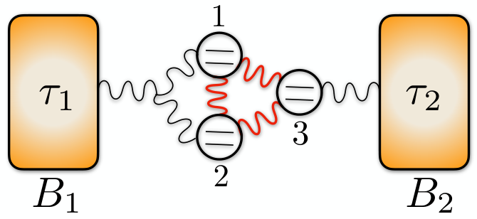
We consider a scenario where at time , qubits and are in thermal equilibrium with a common thermal heat bath, , having a temperature , while the qubit is in thermal equilibrium with the reservoir , which is at temperature (see Fig. 1). We also assume that at , the system Hamiltonian is solely represented by the local Hamiltonian , i.e., at , such that the state of the three-qubit system at is given by . Here,
| (3) |
with being the probability that the qubit is in excited state, and is the partition function of the qubit , being the Boltzmann constant, and being the temperature of the qubit . At , .
For each of the baths, we consider a canonical description of a Markovian thermal bosonic reservoir, constituted of an infinite collection of harmonic oscillators. In this paper, we assume that both of the bosonic baths are characterized by Ohmic spectral functions, given by corresponding to the bath , where is the dimensionless qubit-bath interaction strength, and is a cutoff frequency, identical for both of the baths, which leads to a bath memory time . We work in the Markovian regime, with a value of large enough such that the bath memory time is much smaller than all other relevant time scales. The Hamiltonian for the bath , , is given by
| (4) |
where is the bosonic creation (annihilation) operator corresponding to the mode of the bath , having units of , and is the maximum frequency of the bath . is a constant having the unit of frequency. In the situation described in Fig. 1, the full bath Hamiltonian is given by .
The system-bath coupling considered in the above set-up is given by , where denotes the interaction between the bath , , and the system. As depicted in Fig. 1, the bath interacts with qubits and , while the bath interacts with the qubit only. The qubit-bath interaction Hamiltonian , therefore, is given by
| (5) |
where the “2” in the subscript indicates that the interaction Hamiltonian is constituted of two-body interaction terms between the qubit and the bosonic modes of the bath . On the other hand, reads
| (6) |
with
| (7) | |||||
Here, the Hamiltonians , , represent interactions between qubits and with the bosonic bath modes of bath via -body interaction terms, and are the relative strengths of and with respect to , with , and with . The presence of and gives us a handle to tune the strengths of three- and four-body interactions, relative to the other terms in the Hamiltonian. The Hamiltonian represents the interaction between the qubit pair and a common bosonic mode of the bath via the number operator, and is a natural consequence of having a single bath interacting with the two qubits and . The full Hamiltonian representing the closed system constituted of the three-qubit system and the two baths can, therefore, be represented as
We point out here that in the absence of the three- and four-body interaction terms (i.e., ), the common effect of the bath on the qubits and does not come into consideration, and the setup behaves qualitatively similar to a three-qubit three-bath construction of a quantum absorption refrigerator (for example Das et al. 2019).
Note: The interaction Hamiltonian represents a four-body interaction between the qubit pair and two different bosonic modes of the bath . There are different possibilities of four-body interactions between the qubits , , and the bath modes. We choose one such possibility as the form of (Eq. (7)) in order to check whether the presence of a four-body interaction term can affect the behavior of the model in a significant way. In principle, one can include all such four-body interaction terms obeying the energy conservation principle.
II.1 Quantum Master Equation and Lindblad Operators
If the interaction of strength among the three qubits is turned on for , the system undergoes a dynamics according to the quantum master equation (QME) in the Lindblad form Breuer and Petruccione 2002; Rivas and Huelga 2012,
| (9) |
where is the non-unitary term determined according to the type of the thermal baths attached to the system, and the interactions of the thermal baths with the system. The general form of the Lindblad superoperator is of the form
| (10) |
where is a rate which may or may not depend on the energy of the system, and is a Lindblad operator Breuer and Petruccione 2002; Rivas and Huelga 2012 corresponding to a process for qubit due to its reservoir and occurring at the rate , being a process index. Here and in the rest of the paper, we consider the dimensionless time in units of , the dimensionless energies , and in units of , and the dimensionless temperatures , , and to be in units of , where and are the actual time and the absolute temperature, and is an arbitrary constant having the dimension of energy determined according to the experimental setup used to implement the total Hamiltonian . We also assume Markovian system-bath interaction.
The form of the Lindblad operators can be derived by going over to the interaction picture generated by , and successively applying Born Markov, and rotating-wave approximations Breuer and Petruccione 2002; Rivas and Huelga 2012. In the situation where , the rotating-wave approximation is valid if and only if the typical energy differences of the system Breuer and Petruccione 2002; Rivas and Huelga 2012; Correa et al. 2013; Mitchison et al. 2015. In this scenario, the nonunitary term in Eq. (9) can be written as
| (11) | |||||
where denotes the bath index, and is the set of Lindblad operators corresponding to the transitions due to the bath between the eigenstates of having energy-gap , where the transitions happen at the rates . Determination of is equivalent to decomposing the system operators from the system-bath interaction terms , , , in into eigenoperators corresponding to energy of . All the Lindblad operators are non-Hermitian, satisfying , and are defined as
| (12) |
where , are non-degenerate eigenstates of with energies , , respectively, and . The explicit forms of the Lindblad superoperators are obtained from these expressions by using the eigenvectors of given by
| (13) |
where
| (14) |
with and , while the eigenenergies corresponding to these states are
| (15) |
with .
III Performance as a refrigerator
We now discuss the performance of the three-qubit system described by the Hamiltonian interacting with two reservoirs (see Sec. II) as a quantum refrigerator, where the local temperature of one of the qubits is lowered as an effect of the dynamics of the system. Note that the availability of the two baths and of temperatures and (), respectively, implies that the temperature of a chosen qubit can always be lowered to by keeping it in equilibrium with the bath . Therefore, operation of the machine as a refrigerator for one of the qubits is beneficial if and only if the temperature of the qubit can be lowered below during the dynamics. In the subsequent discussions, we shall demonstrate that this is indeed the case for the three-qubit two-bath setup discussed in Sec. II.
III.1 Working principle
At , the three-qubit system is in contact with the thermal reservoirs and as shown in Fig. 1. Let us denote the probabilities of finding the system in the energy eigenstates and , corresponding to the energy eigenvalues and , by and , respectively. When the interaction term in the system Hamiltonian is turned on, it incorporates a transition between the states and . We begin by assuming the weak-coupling regime of operation, given by , ensuring that the energy eigenvalues and eigenstates of are not drastically modified once the interaction Hamiltonian is turned on (for , and ). We also assume the energy-preserving interactions between the qubits; i.e., we require that commutes with , which requires that , i.e., . In this scenario, if the probability of the transition can be increased (i.e., ), it may lead to a cooling of qubit in the sense that the population of the ground state of qubit increases due to a transfer of excitation from qubit to either qubit , or qubit , or both. The qubit among and receiving the transferred energy undergoes a heating by an increase in the population of its excited state.
For , one can write and explicitly in terms of the energies of the individual qubits and their equilibrium temperatures as
| (16) |
where is the partition function for qubit (see Eq. (3) and subsequent discussions). It is clear from Eq. (16) that for , thereby prohibiting any transition between the energy levels and . Let us assume that , so that . Under this condition, we note the following important points.
- 1.
For , , forbidding a transition between the energy levels and . Therefore, no cooling of either of the qubits or takes place, which is consistent with the symmetry of the setup.
- 2.
For (), (), implying a cooling of qubit (qubit ).
- 3.
Note that a cooling (heating) of qubit takes place for (). Therefore, provides a situation where two out of the three qubits may undergo cooling when the interaction Hamiltonian is turned on.
On the other hand, for , , implying () for (), and the algorithmic cooling and heating of the different qubits occur accordingly.
We point out here that although the above consideration of algorithmic cooling or heating of individual qubits indicates the trend of the temperature of the qubits when the dynamics is started by turning on , it does not predict whether an overall cooling or heating of the chosen qubit will occur once the system reaches its steady state. (Similarly, it is difficult to predict - without following the actual evolution - the possibility of cooling in the strong-coupling regime.) The steady state of the system is a result of the initial state of the system, the system Hamiltonian, the types of the bath, as well as the specific form of the qubit-bath interactions. Note here that a three-qubit quantum refrigerator can also be constructed using three thermal baths instead of two (for example, see Linden et al. 2010; Correa et al. 2013; Mitchison et al. 2015). A steady-state cooling of qubit occurs under the weak- as well as strong-coupling condition of the three-qubit three-bath quantum refrigerator Correa et al. 2013; Mitchison et al. 2015 using bosonic thermal baths. We shall discuss the salient features of these machines, and the specific differences between their properties and the properties of the three-qubit two-bath refrigerator model in subsequent sections.
III.2 Dynamics of cold-qubit temperature

Once the interaction of strength among the three qubits is turned on for , the system is out of equilibrium and undergoes a dynamics according to Eq. (11). A cooling of the qubit, say, , occurs at a finite time instant during the evolution if the temperature . Since the Markovian qubit-bath interactions do not generate coherence in the system, a local temperature of qubit can be defined using the fact that the local density matrices of the individual qubits are always diagonal during the evolution of the system as well as in the steady state. Considering the diagonal form given in Eq. (3) for the state of qubit during the dynamics, its temperature, as a function of time, is given by
| (17) |
where , being the three-qubit state as a function of time according to the evolution of the system. Note that the local temperatures of qubits and can also be defined using equations similar to Eq. (17).
We fix , and focus on the dynamics of the temperature of qubit , which we refer to as the cold qubit from here onward. We solve the QME numerically using the Runge-Kutta 4th-order method, and determine the quantum state of the system as a function of the system as well as system-bath interaction parameters, and time. The temperature of the cold qubit, , as a function of time can be derived using Eq. (17). We consider the steady state of the dynamics of the cold qubit temperature to be achieved when
| (18) |
for a finite time interval . We have chosen , and for all our computations reported in this paper. Let the criterion defined in Eq. (18) be satisfied for the first time during the dynamics at the time . Then the system is considered to have achieved steady state at time , and the steady-state temperature of the cold qubit is given by . We consider a steady-state cooling (SSC) to be the scenario where the dynamics of the system leads to a steady-state temperature, , of the cold qubit which is less than its initial temperature, . In this situation, the qubit represents the object to be cooled, and the rest of the system and the reservoirs construct the refrigerator that dynamically takes the object to a temperature lower than its initial temperature, and keeps it at the lowered temperature as . On the other hand, a transient cooling (TC) of the cold qubit takes place if at a time . Such transient cooling can happen for .
III.2.1 Refrigeration with
We first consider a situation where the interaction between the qubits , and the bath is determined only by the two-body interaction term ( in Eq. ()). The temperature of the cold qubit may exhibit a variety of dynamics. However, subject to cooling occurring in qubit , its dynamic profiles can, in general, be categorized into three types, namely, S1; when SSC is better than TC; S2, when TC is better than SSC, and S3. when TC takes place without an SSC. Let us assume that is the minimum temperature achieved by the cold qubit during transient dynamics for . Using and , the three scenarios for cooling of qubit can be described as follows:
- S1.
SSC better than TC. This situation can be characterized by , and assuming continuity, .
- S2.
TC better than SSC. This refers to a cold qubit dynamics with .
- S3.
TC without SSC. In the third scenario, only transient cooling occurs with no or negligible SSC, i.e., .
We demonstrate these three types of temperature dynamics for the qubit in panels (a) and (d) of Fig. 2, where we keep and at zero values. The values of the energies of the individual qubits, the temperatures of the baths, and the cut-off frequency are fixed at , , and for demonstration. Unless otherwise mentioned, we keep these values fixed throughout the paper. The values of the rate constants, and , are determined from the energies of the individual qubits as well as the temperatures of the thermal reservoirs (see Appendix A.1). For demonstration, we choose two different values of the qubit-qubit interaction strength , representing the weak- and the strong-coupling operating regimes of the machine, such that the rotating wave approximation remains valid in both cases. Unless otherwise mentioned, we use these two values of as representative of the two regimes in all our demonstrations in this paper. The oscillations in the transient dynamics of the cold-qubit temperature increase with an increase in the value of (see panels (a) and (d) of Fig. 2), implying that a steady-state cooling can, in principle, be achieved without an oscillatory dynamics in the strong-coupling regime when is high enough (cf. Mitchison et al. 2015 for the similar dynamics in the case of a three-qubit three-bath refrigerator).
Note that the different types of cooling of qubit reported above are qualitatively similar to the dynamics of cold-qubit temperature obtained in Das et al. 2019, where a three-qubit three-bath setup of the refrigerator was used. As already mentioned in Sec. II, the reason behind such similarity is the absence of the common effect of the bath due to the absence of the few-body interaction terms in the system-bath interaction. Note also that as the qubit pair, and 2, is interacting with a common bath, it is difficult to conceptualize and determine the direction of heat flow from or to either of these qubits, and to explain the cooling process of the individual qubits accordingly. Nevertheless, we observe that a local cooling occurs in the qubit during the dynamics of the three-qubit system – its indication being a reduction in the value of over time. Therefore, in the subsequent sections of this paper, we will refer the cooling of qubit as “local” cooling.
III.2.2 Better local cooling in the presence of three-body interaction
We now investigate the effect of the three-body interaction term in the interaction between the qubits , , and the bath , which is crucial in incorporating the effect of the simultaneous interaction of a common bath mode with both the qubits and . Note that for and , the effect of in the total Hamiltonian (see Eq. ()) dominates, while for , the leading term in the total Hamiltonian is . However, note that a nonzero value of also leads to non-zero transition rates (see Appendix A.1), and contributes to it as . In order to preserve the validity of the rotating-wave approximation, can only be increased up to a maximum possible value . In the parameter space of the three-qubit quantum refrigerator model constituted of two baths, is a function of , , , , and (see Eq. (35)). As the rotating-wave approximation sets upper bounds on the values of the , upper bounds are set on the and . The expressions of and are given in Eqs. (35) and (39), respectively. For all our demonstrations, we choose , so that for the weak- and for the strong-coupling regimes, ensuring that has a sufficiently low value compared to the corresponding values of , and therefore satisfying the rotating-wave approximation. An increase in the value of results in being comparable to , thereby violating the rotating-wave approximation.
In Figs. 2(b)-(c) and Figs. 2(e)-(f), we depict the effect of increasing on the dynamics of the cold-qubit temperature for the weak- and strong-coupling regimes, respectively, while keeping the strength of the four-body interaction term zero (). It is clear from the figures that the steady-state temperature of the cold qubit is significantly lowered from its value at for a non-zero strength of . This effect of the three-body interaction term is advantageous particularly when one is forced to work in the parameter regime where the dynamics is of S2 or S3 type for , , although a local steady-state cooling of qubit is desired. The effect of a non-zero is more prominent in the strong-coupling regime of operation of the three-qubit quantum refrigerator with two baths. This is clearly seen from Figs. 3(a)-(b), where we plot the variation of the steady-state temperature of the cold qubit as a function of in the (a) weak- and (b) strong-coupling operating region, keeping . Note that
- (i)
the effect of the three-body interaction on the steady-state temperature of the type-S1 dynamics is negligible, while considerable lowering of takes place with increasing for type-S2 and type-S3 dynamics; and
- (ii)
when the three-body interaction term is dominating in the total Hamiltonian and the four-body interaction term is absent (i.e., , ), the steady-state temperature of qubit corresponding to both type-S2 and type-S3 dynamics tend to have identical behavior qualitatively as well as quantitatively with increasing .
At this point, it is logical to ask how varies with the system parameters and the temperatures of the baths, when the qubit-bath interaction corresponding to the bath has only two-body (), and two-body as well as three-body () interactions. As discussed in Sec. III.1, the temperature of qubit does not decrease unless . However, in the absence of the three-body interaction term (i.e., for ), has a non-monotonic variation with increasing in both weak- as well as strong-coupling regimes of the refrigerator. The variation increases in both regimes as the strength of the three-body interaction term increases [see Figs. 4(a) and 4(b)]. With increasing , the values of decreases first, attains a minimum, and then increases again to achieve an almost constant value close to . This implies that an optimum value of exists for a specific value of in order to obtain the maximum possible local steady-state cooling. Increasing beyond the optimum value for a specific value of would decrease the performance of the setup as a refrigerator for qubit , and eventually lead to a situation where almost no local steady-state cooling will be obtained. The minimum value of decreases with increasing while keeping , as depicted clearly in the figure.
In Fig. 4(c), we plot as a function of , where the value of changes from weak-coupling regime to strong-coupling regime, and the values of the parameters are chosen such that the rotating-wave approximation remains valid in both regimes. We investigate both situations where only two-body (), and two- as well as three-body interactions are present in , but the four-body interaction term is absent (). As the figure demonstrates, increases monotonically with , indicating a better local steady-state cooling being favored when the refrigerator is operating with a lower value of . With increasing strength of keeping , decreases for a fixed value of .
We also investigate how the steady-state temperature of qubit varies with the temperatures of the baths and . We find that decreases monotonically with , which is demonstrated in Fig. 5. Note that with increasing and fixed at , the decrease in becomes gradually slower, and at a high-enough value of , becomes almost constant with .
III.2.3 Effects of four-body interaction is negligible
At this point, a natural question is whether the steady-state temperature of the cold qubit continues to decrease as one keeps on adding higher order interaction terms in the qubit-bath interactions corresponding to the bath . To investigate this question, we add a four-body interaction term of the form to (see Eq. ()). As already mentioned in Sec. II, there are different possibilities for the form of the four-body interaction term obeying the energy conservation principle. We choose a specific term among the different possibilities in order to check whether there is a substantial difference in results due to the presence of the four-body interaction in . The strength of the four-body interaction term relative to is taken to be . We find that for a fixed value of , even a very high value of changes only negligibly. This trend is prominent only in the S2-S3 type dynamics (see Figs. 6(b)-(c)). This observation is also supported by the variations of with , , and , with (see Figs. 4-5). A small effect of in the local temperature of the qubit can be understood from the fact that although , similar to , contributes as in the expression of , unlike , depends on the Ohmic spectral function as . Therefore, the values of the transition rates , within the validity of the rotating-wave approximation, become very small, and so is the effect of the four-body interaction term. Since the dependence of the transition rate on and remains the same for all possible forms of the four-body interaction terms, the effect due to other forms of four-body interaction terms is also expected to be negligible.
Fig. 5 also brings forth a rather curious result. For , we get even for negligible or vanishing ; i.e., local cooling of qubit 1 occurs even without a temperature difference between the two baths. This finding motivates the question as to whether a local cooling of qubit 1 is possible if one works with a single bath and few-body interaction terms, which we briefly discuss in the succeeding subsection.
III.2.4 Three-qubit refrigerator with a single bath?
Here we assume that a system of three qubits is interacting with a common bosonic bath at temperature , characterized by the Ohmic spectral function, , where is the cut-off frequency (see Sec. II). The local Hamiltonian and the interaction Hamiltonian are as in Eqs. (1) and (2), respectively, where we consider only two-body and three-body interaction terms for the qubit-bath interaction (i.e., ). The Hamiltonian of the common bath is given by
| (19) |
while the qubit-bath interaction Hamiltonian is
| (20) |
with
| (21) | |||||
such that the total Hamiltonian for the system-environment duo is represented as
| (22) |
In the presence of only two-body interaction between the qubits and the bath (i.e., with ), none of the qubits is cooled, which is in contrast with the local cooling of qubit 1 in the case of the three-qubit two-bath model (see Figs. 2(a) and (d)). When , local cooling of qubit 1 takes place, as depicted in Fig. 7. For both weak as well as strong coupling, an increase in the value of results in a local cooling of the first qubit. The thermodynamic consistency of this setup, as well as the setup with two baths of possibly equal temperatures, is commented on in the following section.
III.3 Thermodynamic consistency of single- and two-bath refrigerators
For a quantum thermal machine described by a quantum master equation, the validity of the second law of thermodynamics is determined by the balance equation of entropy production rate,
| (23) |
where is the entropy of the system, quantifies the flow of entropy (heat) from the system to the bath , with being the Boltzmann constant, is the absolute temperature of the bath , and is the source term quantifying the entropy production rate of the system. It has been shown that the second law of thermodynamics is always valid for global master equations, but seems to be violated in cases of local master equations where the Lindblad operators are obtained by considering transitions between eigenstates of local Hamiltonians of the individual subsystems (e.g., in Eq. (1)) Barra 2015; *Strasberg2017; *De_Chiara2018. Therefore, the usual definition of the heat current, viz. , where is the dissipating term corresponding to the bath and , is the local Hamiltonian, may not be a proper definition to check the validity of Eq. (23), and the actual expression of the heat currents has to be carefully determined Hewgill et al. 2021. In the single- and two-bath refrigerator setups, we have obtained the Lindblad operators by considering transitions between eigenstates of the total system Hamiltonian, , thereby following the global approach of the master equation. This implies that the balance equation is always valid in our case. The excess terms that appear due to the consideration of the “nonlocal” term, , may also be incorporated into the entropy production rate term on the right-hand side of Eq. (23), to be interpreted as “excess source” terms in the thermodynamics of the system. The weak-coupling Lindblad master equation sometimes fails to describe the stationary nonequilibrium properties, and this problem can also be resolved by constructing the master equation in a different way (see Wichterich et al. 2007).
IV Refrigeration using reset model of qubit-bath interaction
In order to check whether the features of the local steady-state cooling obtained in the three-qubit refrigerator model constituted using two thermal baths are artifacts of the specific qubit-bath interactions used in this paper, or are generic properties of the two-bath construction, we consider a second and rather well-studied model of qubit-bath interaction, namely, the reset model Linden et al. 2010; Correa et al. 2013; Mitchison et al. 2015; Das et al. 2019. We assume that at each time step, the bath induces a probabilistic reset on the attached qubit or group of qubits, such that the state of the qubit or the group of qubits is replaced by the initial () thermal state. In the two-bath setup described in Fig. 1, the dynamical term (Eq. (9)) can be written as (cf. Linden et al. 2010 for the three-bath setup)
| (24) | |||||
where and are respectively the thermal states of the qubit-pair and the qubit at , and the states are given in Eq. (3). The qubit-bath interaction parameters , , are the probability densities per unit time, which provide the probability with which the reset operation is performed by the bath, and thereby provide a figure of merit of the quality of insulation of the qubit(s) from the bath(s). Here, we have assumed that the bath resets the states of the qubits and simultaneously. It can be shown by straightforward algebra that the Lindblad operators corresponding to the dynamics described by Eq. (24) are of the form and , with and , where the operators have the form , , , and . The transition rates (in Eq. (10)) corresponding to the transformations due to the operators have two components, (i) the qubit-bath interaction parameter , and (ii) the temperature-dependent component , , with , , , and , which are fully determined by the thermal bath. In the case of the Lindblad operators corresponding to the qubit-pair , the transition rates can be obtained as , , , where and have the same form as that of .
The discussion on the working principle of the three-qubit refrigerator (Sec. III.1) is valid also for this model. However, it may not be intuitively clear whether the three types of dynamics of the temperature for the qubit are obtained once the qubit-qubit interaction is turned on. We answer this question affirmatively in this paper. In Fig 8(a), we illustrate an example of the dynamics of the temperature of qubit in the three-qubit two-bath system (Fig. 1), where qubit has undergone dynamics of types S1, S2, and S3 for . The calibration of the temperature of the steady state of qubit in the case of the reset model is qualitatively similar when , , and are chosen as the calibration parameter (see Figs. 8(b)-(d)). We point out here that the use of the reset model as the qubit-bath interaction has the liberty of using any value of the reset probability densities , acting as the qubit-bath interaction parameters, which is in contrast to the case of the bosonic baths where the rotating-wave approximation imposes additional restrictions on the values of the system-, bath-, as well as the qubit-bath-interaction parameters. Therefore, a one-to-one comparison between the reset model and the model considering bosonic baths may not be possible.
V Discussion
We considered a quantum absorption refrigerator constituted of three interacting qubits and two thermal baths, where two of the qubits, including the target qubit for local cooling, are kept in contact with a common reservoir. The interaction between each qubit and its corresponding bath is considered to be Markovian in nature, and we used thermal reservoirs made of an infinite number of quantum harmonic oscillators. The use of the common reservoir results in the presence of three- and four-body interaction terms in the Hamiltonian representing the qubit-bath interactions. We specifically considered a three-body interaction term involving the interaction between the spin degree of freedom of the qubit with the number operator corresponding to a specific bosonic mode, and a four-body interaction term constituted of the spin degrees of freedom of the qubits and two different bath modes of the common bath.
We first studied a situation where the few-body interactions are absent, and showed that the three-qubit two-bath setup can indeed lead to a local steady-state cooling of one of the qubits connected to the common bath. We also showed that similar to a three-qubit three-bath refrigerator, a parameter regime exists also for the two-bath setup where little or no local steady-state cooling is achieved, thereby making the parameter regime disadvantageous for the functioning of the machine. However, in such situations, the few-body interaction terms play an important role. We demonstrated that in these parameter regions, upon turning on the strengths of the three- and four-body interaction terms, the steady-state temperature of the cold qubit decreases monotonically with an increase in the interaction strengths, resulting in substantial local steady-state cooling. Our findings suggest that the effect of the three-body interaction term in reducing the steady-state temperature is considerably higher compared to the four-body interaction term. We also explained the reason behind the effect of four- and higher than four-body interactions on the local steady-state cooling being so small compared to the three- and two-body terms. We further demonstrated that our setup can perform as a refrigerator even when the qubit-bath interaction is replaced by the widely studied reset model.
It is interesting to investigate the possible connections between the local temperature of the individual qubits and the different types of quantum correlations among the qubits in the system. We have checked that in the three-qubit two-bath setup of the quantum refrigerator, bipartite entanglement Horodecki et al. 2009, as measured by negativity Peres 1996; Horodecki et al. 1996; Vidal and Werner 2002, in the partition of the three-qubit system remains at zero irrespective of the values of the system, the bath, and the system-bath interaction parameters as well as in the presence and absence of the few-body interaction terms in the qubit-bath interactions. The quantum coherence Baumgratz et al. 2014 of qubit , computed using the reduced state of qubit which is obtained by tracing out the rest of the qubits, also exhibits similar behavior in the eigenbasis of the local Hamiltonian. However, the quantum coherence for the three-qubit system in the computational multi-orthogonal product basis, and the mutual information Witten in the bipartition of the three-qubit system, oscillates at first, and then stabilizes to a nonzero value – a behavior that is qualitatively similar to the dynamics of the total mutual information in the three-qubit three-bath setup Das et al. 2019. These features also remain unchanged irrespective of whether the three- and four-body terms are present in the qubit-bath interactions.
Acknowledgements.
We acknowledge computations performed at the cluster computing facility of Harish-Chandra Research Institute (HRI), India. S.D. acknowledges support from the Munich Center for Quantum Science and Technology. A.K.P. thanks HRI, India, for hospitality during his visits, and acknowledges IIT Palakkad for support from a seed Grant. The authors from HRI acknowledge support from the Department of Science and Technology, Government of India, through the QuEST grant (Grants No. DST/ICPS/QUST/Theme-1/2019/23 and No. DST/ICPS/QUST/Theme-3/2019/120).Appendix A Explicit forms of Lindblad operators and transition rates
A.1 Lindblad operators
In order to determine the explicit forms of the Lindblad operators, we note that the eigenstates of and the corresponding eigenenergies are given by Eqs. (II.1) and (II.1). We first consider the Lindblad operators corresponding to the bath (i.e., for transitions corresponding to qubit-pair ). As per Eqs. (12) and (13), there are possible transition channels for the qubit pair , among which the ones for positive energy gaps are given by
| (25) |
with . The transition channels corresponding to the negative energy gaps, , are obtained from , . Similarly, there are possible transition channels for qubit connected to the bath , and the ones corresponding to positive energy gaps are given by
| (26) |
while the collapse operators corresponding to the negative energy gaps are given by .
A.2 Transition rates
The transition rates can be expressed in terms of the bath operators corresponding to the bath as Rivas and Huelga 2012
| (27) |
with being the state of bath and corresponding to two-, three-, and four-body interaction terms. Here, and are the indices that run from to and construct a matrix for each transition energy . We denote the bath operators corresponding to the bath by , while is the bath operator for the transition energy , with
| (28) |
For the two-body interaction terms, and , the bath operators, , are
| (29) |
and the operators (, ) are given by
| (30) |
The corresponding transition rates, for , are given by
| (31) |
Similarly, for the interaction term , the bath operators are
| (32) |
and
| (33) |
such that
| (34) | |||||
So can be represented as
| (35) | |||||
For the four-body interaction term , the bath operators are
and the operators can be written as
| (37) |
where . Substitution of Eqs. () and (37) in Eq. (27) and subsequent algebra leads to
| (38) |
and takes the form
| (39) |
where is the Bose-Einstein distribution. Note that in order to take care of the non-analyticity of at , we choose such that is finite.
References
- Gemmer et al. (2004) G. Gemmer, M. Michel, and G. Mahler, Quantum Thermodynamics (Springer, New York, 2004).
- Kosloff (2013) R. Kosloff, Entropy 15, 2100 (2013).
- Gelbwaser-Klimovsky et al. (2015) D. Gelbwaser-Klimovsky, W. Niedenzu, and G. Kurizki, Adv. At. Mol. Opt. Phys. 64, 329 (2015).
- Misra et al. (2015) A. Misra, U. Singh, M. N. Bera, and A. K. Rajagopal, Phys. Rev. E 92, 042161 (2015).
- Millen and Xuereb (2016) J. Millen and A. Xuereb, New Journal of Physics 18, 011002 (2016).
- Benenti et al. (2017) G. Benenti, G. Casati, K. Saito, and R. S. Whitney, Phys. Rep. 694, 1 (2017).
- Deffner and Campbell (2019) S. Deffner and S. Campbell, Quantum Thermodynamics, 2053-2571 (Morgan and Claypool Publishers, 2019).
- Vinjanampathy and Anders (2016) S. Vinjanampathy and J. Anders, Contemporary Physics 57, 545 (2016).
- Goold et al. (2016) J. Goold, M. Huber, A. Riera, L. del Rio, and P. Skrzypczyk, Journal of Physics A: Mathematical and Theoretical 49, 143001 (2016).
- Allahverdyan and Nieuwenhuizen (2000) A. E. Allahverdyan and T. M. Nieuwenhuizen, Phys. Rev. Lett. 85, 1799 (2000).
- Brandão et al. (2015) F. Brandão, M. Horodecki, N. Ng, J. Oppenheim, and S. Wehner, Proceedings of the National Academy of Sciences 112, 3275 (2015).
- Gardas and Deffner (2015) B. Gardas and S. Deffner, Phys. Rev. E 92, 042126 (2015).
- Palao et al. (2001) J. P. Palao, R. Kosloff, and J. M. Gordon, Phys. Rev. E 64, 056130 (2001).
- Feldmann and Kosloff (2003) T. Feldmann and R. Kosloff, Phys. Rev. E 68, 016101 (2003).
- Nimmrichter et al. (2018) S. Nimmrichter, A. Roulet, and V. Scarani, “Quantum rotor engines,” in Thermodynamics in the Quantum Regime: Fundamental Aspects and New Directions, edited by F. Binder, L. A. Correa, C. Gogolin, J. Anders, and G. Adesso (Springer International Publishing, Cham, 2018) pp. 227–245.
- Kosloff and Levy (2014) R. Kosloff and A. Levy, Annual Review of Physical Chemistry 65, 365 (2014).
- Uzdin et al. (2015) R. Uzdin, A. Levy, and R. Kosloff, Phys. Rev. X 5, 031044 (2015).
- Levy and Kosloff (2012) A. Levy and R. Kosloff, Phys. Rev. Lett. 108, 070604 (2012).
- Clivaz et al. (2019) F. Clivaz, R. Silva, G. Haack, J. B. Brask, N. Brunner, and M. Huber, Phys. Rev. Lett. 123, 170605 (2019).
- Mitchison (2019) M. T. Mitchison, Contemporary Physics 60, 164 (2019).
- (21) S. Bhattacharjee and A. Dutta, arXiv:2008.07889 .
- Geva and Kosloff (1992) E. Geva and R. Kosloff, J. Chem. Phys. 97, 4398 (1992).
- Feldmann and Kosloff (2000) T. Feldmann and R. Kosloff, Phys. Rev. E 61, 4774 (2000).
- Ng et al. (2017) N. H. Y. Ng, M. P. Woods, and S. Wehner, New Journal of Physics 19, 113005 (2017).
- Niedenzu et al. (2018) W. Niedenzu, V. Mukherjee, A. Ghosh, A. G. Kofman, and G. Kurizki, Nature Communications 9, 165 (2018).
- Xu et al. (2018) Y. Y. Xu, B. Chen, and J. Liu, Phys. Rev. E 97, 022130 (2018).
- Huber et al. (2015) M. Huber, M. Perarnau-Llobet, K. V. Hovhannisyan, P. Skrzypczyk, C. Klöckl, N. Brunner, and A. Acín, New Journal of Physics 17, 065008 (2015).
- Lostaglio et al. (2015) M. Lostaglio, D. Jennings, and T. Rudolph, Nature Communications 6, 6383 (2015).
- Ikonen et al. (2017) J. Ikonen, J. Salmilehto, and M. Möttönen, npj Quantum Information 3, 17 (2017).
- Campisi et al. (2015) M. Campisi, J. Pekola, and R. Fazio, New Journal of Physics 17, 035012 (2015).
- D’Alessio et al. (2016) L. D’Alessio, Y. Kafri, A. Polkovnikov, and M. Rigol, Advances in Physics 65, 239 (2016).
- Gour et al. (2015) G. Gour, M. P. Müller, V. Narasimhachar, R. W. Spekkens, and N. Y. Halpern, Phys. Rep. 583, 1 (2015).
- Dorner et al. (2012) R. Dorner, J. Goold, C. Cormick, M. Paternostro, and V. Vedral, Phys. Rev. Lett. 109, 160601 (2012).
- Mehboudi et al. (2015) M. Mehboudi, M. Moreno-Cardoner, G. D. Chiara, and A. Sanpera, New Journal of Physics 17, 055020 (2015).
- Reimann (2015) P. Reimann, New Journal of Physics 17, 055025 (2015).
- Eisert et al. (2015) J. Eisert, M. Friesdorf, and C. Gogolin, Nature Physics 11, 124 (2015).
- Gogolin and Eisert (2016) C. Gogolin and J. Eisert, Reports on Progress in Physics 79, 056001 (2016).
- Skelt et al. (2019) A. H. Skelt, K. Zawadzki, and I. D’Amico, Journal of Physics A: Mathematical and Theoretical 52, 485304 (2019).
- Giazotto et al. (2006) F. Giazotto, T. T. Heikkilä, A. Luukanen, A. M. Savin, and J. P. Pekola, Rev. Mod. Phys. 78, 217 (2006).
- Abah et al. (2012) O. Abah, J. Roßnagel, G. Jacob, S. Deffner, F. Schmidt-Kaler, K. Singer, and E. Lutz, Phys. Rev. Lett. 109, 203006 (2012).
- Roßnagel et al. (2016) J. Roßnagel, S. T. Dawkins, K. N. Tolazzi, O. Abah, E. Lutz, F. Schmidt-Kaler, and K. Singer, Science 352, 325 (2016).
- Peterson et al. (2019) J. P. S. Peterson, T. B. Batalhão, M. Herrera, A. M. Souza, R. S. Sarthour, I. S. Oliveira, and R. M. Serra, Phys. Rev. Lett. 123, 240601 (2019).
- Karimi and Pekola (2016) B. Karimi and J. P. Pekola, Phys. Rev. B 94, 184503 (2016).
- Hardal et al. (2017) A. U. C. Hardal, N. Aslan, C. M. Wilson, and O. E. Müstecaplıoğlu, Phys. Rev. E 96, 062120 (2017).
- Manikandan et al. (2019) S. K. Manikandan, F. Giazotto, and A. N. Jordan, Phys. Rev. Applied 11, 054034 (2019).
- Linden et al. (2010) N. Linden, S. Popescu, and P. Skrzypczyk, Phys. Rev. Lett. 105, 130401 (2010).
- Skrzypczyk et al. (2011) P. Skrzypczyk, N. Brunner, N. Linden, and S. Popescu, Journal of Physics A: Mathematical and Theoretical 44, 492002 (2011).
- Brunner et al. (2012) N. Brunner, N. Linden, S. Popescu, and P. Skrzypczyk, Phys. Rev. E 85, 051117 (2012).
- Brunner et al. (2014) N. Brunner, M. Huber, N. Linden, S. Popescu, R. Silva, and P. Skrzypczyk, Phys. Rev. E 89, 032115 (2014).
- Brask and Brunner (2015) J. B. Brask and N. Brunner, Phys. Rev. E 92, 062101 (2015).
- Correa et al. (2013) L. A. Correa, J. P. Palao, G. Adesso, and D. Alonso, Phys. Rev. E 87, 042131 (2013).
- Correa et al. (2014) L. A. Correa, J. Palao, D. Alonso, and G. Adesso, Scientific Reports 4, 3949 (2014).
- Silva et al. (2015) R. Silva, P. Skrzypczyk, and N. Brunner, Phys. Rev. E 92, 012136 (2015).
- Erdman et al. (2018) P. A. Erdman, B. Bhandari, R. Fazio, J. P. Pekola, and F. Taddei, Phys. Rev. B 98, 045433 (2018).
- Naseem et al. (2020) M. T. Naseem, A. Misra, and Özgür E Müstecaplıoğlu, Quantum Science and Technology 5, 035006 (2020).
- Mitchison et al. (2015) M. T. Mitchison, M. P. Woods, J. Prior, and M. Huber, New Journal of Physics 17, 115013 (2015).
- Das et al. (2019) S. Das, A. Misra, A. K. Pal, A. Sen(De), and U. Sen, EPL (Europhysics Letters) 125, 20007 (2019).
- Man and Xia (2017) Z.-X. Man and Y.-J. Xia, Phys. Rev. E 96, 012122 (2017).
- Friedman and Segal (2019) H. M. Friedman and D. Segal, Phys. Rev. E 100, 062112 (2019).
- Wang et al. (2015) J. Wang, Y. Lai, Z. Ye, J. He, Y. Ma, and Q. Liao, Phys. Rev. E 91, 050102 (2015).
- He et al. (2017) Z.-c. He, X.-y. Huang, and C.-s. Yu, Phys. Rev. E 96, 052126 (2017).
- Du and Zhang (2018) J.-Y. Du and F.-L. Zhang, New Journal of Physics 20, 063005 (2018).
- Mukhopadhyay et al. (2018) C. Mukhopadhyay, A. Misra, S. Bhattacharya, and A. K. Pati, Phys. Rev. E 97, 062116 (2018).
- Seah et al. (2018) S. Seah, S. Nimmrichter, and V. Scarani, Phys. Rev. E 98, 012131 (2018).
- Barra and Lledó (2018) F. Barra and C. Lledó, The European Physical Journal Special Topics 227, 231 (2018).
- Hewgill et al. (2020) A. Hewgill, J. O. González, J. P. Palao, D. Alonso, A. Ferraro, and G. De Chiara, Phys. Rev. E 101, 012109 (2020).
- Venturelli et al. (2013) D. Venturelli, R. Fazio, and V. Giovannetti, Phys. Rev. Lett. 110, 256801 (2013).
- Hofer et al. (2016) P. P. Hofer, M. Perarnau-Llobet, J. B. Brask, R. Silva, M. Huber, and N. Brunner, Phys. Rev. B 94, 235420 (2016).
- Mitchison et al. (2016) M. T. Mitchison, M. Huber, J. Prior, M. P. Woods, and M. B. Plenio, Quantum Science and Technology 1, 015001 (2016).
- Mitchison and Potts (2018) M. T. Mitchison and P. P. Potts, “Physical implementations of quantum absorption refrigerators,” in Thermodynamics in the Quantum Regime: Fundamental Aspects and New Directions, edited by F. Binder, L. A. Correa, C. Gogolin, J. Anders, and G. Adesso (Springer International Publishing, Cham, 2018) pp. 149–174.
- Maslennikov et al. (2019) G. Maslennikov, S. Ding, R. Hablützel, J. Gan, A. Roulet, S. Nimmrichter, J. Dai, V. Scarani, and D. Matsukevich, Nature Communications 10, 202 (2019).
- Basilewitsch et al. (2019) D. Basilewitsch, F. Cosco, N. L. Gullo, M. Möttönen, T. Ala-Nissilä, C. P. Koch, and S. Maniscalco, New Journal of Physics 21, 093054 (2019).
- Poyatos et al. (1996) J. F. Poyatos, J. I. Cirac, and P. Zoller, Phys. Rev. Lett. 77, 4728 (1996).
- Myatt et al. (2000) C. J. Myatt, B. E. King, Q. A. Turchette, C. A. Sackett, D. Kielpinski, W. M. Itano, C. Monroe, and D. J. Wineland, Nature 403, 269 (2000).
- Manzano et al. (2019) G. Manzano, G.-L. Giorgi, R. Fazio, and R. Zambrini, New Journal of Physics 21, 123026 (2019).
- Breuer and Petruccione (2002) H. P. Breuer and F. Petruccione, The Theory of Open Quantum Systems (Oxford University Press, Oxford, 2002).
- Rivas and Huelga (2012) A. Rivas and S. F. Huelga, Open Quantum Systems: An Introduction (SpringerBriefs in Physics, Springer, Spain, 2012).
- Barra (2015) F. Barra, Scientific Reports 5, 14873 (2015).
- Strasberg et al. (2017) P. Strasberg, G. Schaller, T. Brandes, and M. Esposito, Phys. Rev. X 7, 021003 (2017).
- Chiara et al. (2018) G. D. Chiara, G. Landi, A. Hewgill, B. Reid, A. Ferraro, A. J. Roncaglia, and M. Antezza, New Journal of Physics 20, 113024 (2018).
- Hewgill et al. (2021) A. Hewgill, G. De Chiara, and A. Imparato, Phys. Rev. Research 3, 013165 (2021).
- Wichterich et al. (2007) H. Wichterich, M. J. Henrich, H.-P. Breuer, J. Gemmer, and M. Michel, Phys. Rev. E 76, 031115 (2007).
- Horodecki et al. (2009) R. Horodecki, P. Horodecki, M. Horodecki, and K. Horodecki, Rev. Mod. Phys. 81, 865 (2009).
- Peres (1996) A. Peres, Phys. Rev. Lett. 77, 1413 (1996).
- Horodecki et al. (1996) M. Horodecki, P. Horodecki, and R. Horodecki, Phys. Lett. A 223, 1 (1996).
- Vidal and Werner (2002) G. Vidal and R. F. Werner, Phys. Rev. A 65, 032314 (2002).
- Baumgratz et al. (2014) T. Baumgratz, M. Cramer, and M. B. Plenio, Phys. Rev. Lett. 113, 140401 (2014).
- (88) E. Witten, arXiv:1805.11965 .