GAP-net for Snapshot Compressive Imaging
Abstract
Snapshot compressive imaging (SCI) systems aim to capture high-dimensional (D) images in a single shot using 2D detectors. SCI devices include two main parts: a hardware encoder and a software decoder. The hardware encoder typically consists of an (optical) imaging system designed to capture compressed measurements. The software decoder on the other hand refers to a reconstruction algorithm that retrieves the desired high-dimensional signal from those measurements. In this paper, using deep unfolding ideas, we propose an SCI recovery algorithm, namely GAP-net, which unfolds the generalized alternating projection (GAP) algorithm. At each stage, GAP-net passes its current estimate of the desired signal through a trained convolutional neural network (CNN). The CNN operates as a denoiser that projects the estimate back to the desired signal space. For the GAP-net that employs trained auto-encoder-based denoisers, we prove a probabilistic global convergence result. Finally, we investigate the performance of GAP-net in solving video SCI and spectral SCI problems. In both cases, GAP-net demonstrates competitive performance on both synthetic and real data. In addition to having high accuracy and high speed, we show that GAP-net is flexible with respect to signal modulation implying that a trained GAP-net decoder can be applied in different systems. Our code is at https://github.com/mengziyi64/ADMM-net.
Index Terms:
Compressive imaging, Compressive sensing, Deep learning, Generative alternating projection, Snapshot, Convolution neural network, Convergence, DenoisingI Introduction
Recent advances in artificial intelligence and robotics have resulted in an unprecedented demand for computationally-efficient high-dimensional (HD) data capture and processing devices. However, existing optical sensors usually can only directly capture no more than two-dimensional (2D) signals. Capturing 3D or higher dimensional signals remains challenging since sensors that directly perform 3D data acquisition do not yet exist.
In recent years, snapshot compressive imaging (SCI) systems that employ 2D detectors to capture HD (3D) signals have been shown to be a promising solution to address this challenge. Different from conventional cameras, SCI systems perform sampling on a set of consecutive images—video frames (e.g., CACTI [21]) or spectral channels (e.g., CASSI [39])—in accordance with the sensing matrix and integrate these sampled signals along time or spectrum to obtain the final compressed measurements. Using this technique, SCI systems [7, 12, 31] can capture high-speed motion [52, 53] or high-resolution spectral information [40, 54], with low memory, low bandwidth, low power and potentially low cost.
There are two main ingredients in an SCI system: a hardware encoder and a software decoder. The hardware encoder is typically an (optical) imaging system that is designed to capture compressed measurements of the desired signal and the software decoder refers to the algorithm that recovers the desired HD data from those measurements. The underlying principle of the hardware encoder is to modulate the HD data using a speed higher than the capture rate of the camera. To achieve this goal, typically, a coded aperture (binary mask) or some other spatial light modulators is employed. In this paper, we focus on the software decoder, i.e., the reconstruction algorithm, which, until recently, had precluded wide application of SCI due to the slow speed of existing reconstruction methods. Thanks to deep learning, various SCI recovery algorithms based on convolutional neural networks (CNNs) have been developed in recent years [30, 42, 23, 5]. These algorithms significantly speed up the reconstruction process compared to the previous methods. This has paved the way to daily applications of SCI systems.
Reconstruction algorithms for SCI can be divided into four classes as follows: (Refer to Fig. 1.)
- (a)
- (b)
End-to-end CNNs (E2E-CNNs) that are trained with a large amount of training data consisting of measurements and (optionally) masks as input and the ground truth i.e., the underlying desired signal, as output; during testing, feeding the captured measurements into the trained E2E-CNN, it is expected to produce the desired signal instantaneously [27, 24, 5];
- (c)
- (d)
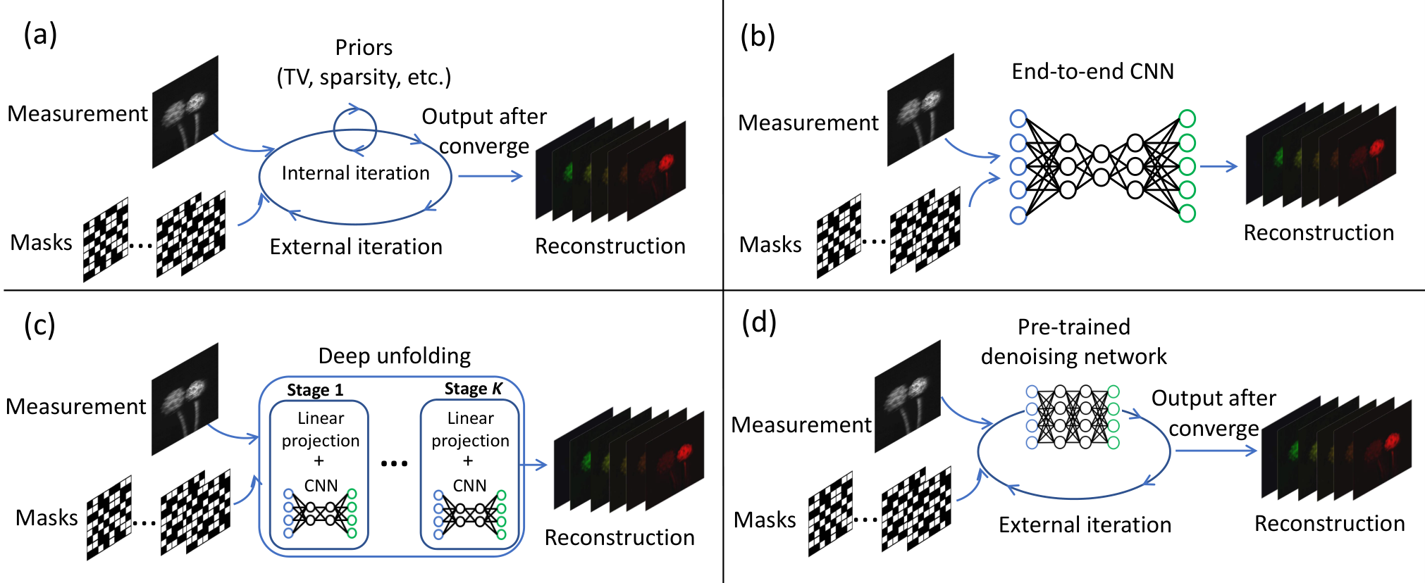
Iterative optimization-based methods have been studied extensively in the literature for a diverse set of priors. The speed and quality of such algorithms are variant, with faster versions (e.g., those using TV [1, 50]) typically not achieving high reconstruction quality, and high performance versions usually being very slow [20]. However, even a relatively fast algorithm of class (a) is currently considerably slower than CNN-based algorithms of classes (b)-(d) [30]. E2E-CNN algorithms require a large training data set, a long training time and large GPU memory. In some applications this is infeasible, for instance when dealing with large-scale data sets [51]. PnP algorithms are flexible and can be used in large-scale data sets, since they do not need to retrain the network. However, their performance is mainly limited by the pre-trained denoising network. For instance, efficient and flexible denoising algorithms for hyperspectral images are not yet available.
I-A Related work
Various optimization-based SCI algorithms, such as TwIST [1], GAP-TV [50], GMM [46, 45] and DeSCI [20], using different priors have been developed. The state-of-the-art algorithm, DeSCI [20], applies weighted nuclear norm minimization [8] of non-local similar patches in video frames into the alternating direction method of multipliers (ADMM) framework [2]. While DeSCI can recover clear images, it takes about two hours for it to recover 8 frames (each of size ), which precludes its wide application. Inspired by the recent successes of deep-learning-based solutions on image restoration [44, 56], in recent years, researchers have explored application of deep learning in computational imaging as well [4, 13, 15, 17, 28, 34]. Deep unfolding (or unrolling) [11] has been used for compressive sensing (CS) and various solvers such as ADMM-net [48], ISTA-net [55] and learned D-AMP [25] have been proposed.11 1 It has been observed in several papers [14] and experiments [20] that AMP does not converge well in SCI applications, due to the special structure of sensing matrix in SCI and ADMM usually outperforms ISTA. Regarding the E2E-CNN, the recurrent neural network (RNN) proposed in [5] can now provide competitive results as DeSCI for video SCI and the best spectral SCI result is obtained by the spectial-spectral model proposed in [23].
Deep unfolding has also been used for video SCI in [18, 9, 22] and spectral SCI [41]. However, these methods are inspired by sparse coding in each stage and the resulting reconstruction quality of real data is low. Furthermore, no convergence guarantees have been established for such algorithms yet. The most recent paper [18] employs a similar idea of using a denoiser at each stage. However, the paper only explores video SCI and provides no theoretical analysis of the proposed method.
Note that existing models were developed either for video SCI or spectral SCI. For instance, it is reasonable to use RNNs in video SCI, but it is not intuitive to apply RNNs to spectral SCI. In this paper, we aim to develop a unified model that works efficiently for both video SCI and spectral SCI.
I-B Contributions of this work
Motivated by the pros and cons of different approaches, in this paper, we propose a deep unfolding SCI recovery algorithm called GAP-net. Here are some key properties of GAP-net that are described in details later:
- •
- •
GAP-net, a recovery algorithm for both video and spectral SCI, treats the trained CNN at each stage of the decoder as a denoising network. This is in the same spirit as learned D-AMP [25], a recovery method for image CS and [18] for video SCI. There exist other SCI recovery algorithms in the literature that are based on deep unfolding. In such methods, the CNN in each stage of the unfolding includes the transformation (implemented by convolutional or fully-connected neural networks) and shrinkage (implemented by ReLU, etc.).
- •
Based on the above denoising perspective, GAP-net is related to the PnP framework for SCI [51]. We theoretically prove and experimentally verify its convergence to the desired result22 2 We observed some error in the proof of the global convergence of PnP-GAP in [51]. Specifically, the lower bound of the second term in Eq. (25) in [51] should be 0. Therefore, the proof of global convergence for PnP-GAP presented in [51] does not hold. The authors have updated the manuscript on arXiv with a local convergence result. In this paper, using concentration of measure tools, we prove global convergence of GAP-net..
- •
GAP-net achieves state-of-the-art (in some cases, competitive) performance in our experimental results done both with synthetic data and real data, in both video SCI and spectral SCI.
II Video SCI and Spectral SCI
Fig. 2 depicts the schematic diagrams of both video (left) and spectral (right) SCI. As mentioned earlier, the underlying principle in both of them is to modulate the datacube using a speed higher than the capture rate of the camera. In video SCI, different modulation solutions, such as a shifting mask [21] and different digital micromirror device (DMD) patterns [12], both of which are active modulation methods, have been proposed. On the other hand, in spectral SCI, the modulation can be implemented by a fixed mask plus a disperser [39], which is a passive modulation approach and thus more power efficient. The key idea is that, using a disperser, a fixed modulation pattern can be shifted to be different for different wavelengths.

II-A Forward Model of Video SCI
Consider a video SCI encoder, where a -frame video is modulated and mapped by sensing matrices (masks) to a single measurement frame as
| (1) |
where denotes the noise; and denote the -th sensing matrix (mask) and the corresponding video frame, respectively; denotes the Hadamard (element-wise) product. Using vectoring operator, define and . Similarly, define as
| (2) |
Using these definitions, the measurement process defined in (1) can be expressed as
| (3) |
Unlike standard CS, the sensing matrix in video SCI is highly structured and sparse. More precisely, it can be written as the concatenation of diagonal matrices as
| (4) |
where, for , with . Here, the sampling rate is equal to . It has been proven in [14] that, if the signal is structured enough, there exist SCI recovery algorithms with bounded reconstruction error, even for .
II-B Forward Model of Spectral SCI
Recall Fig. 2(b) which shows a schematic diagram of an spectral SCI system. Let and denote the original spectral cube and the fixed mask modulation, respectively. After scene passes through the mask, let denote its modulated version, in which images at different wavelengths are modulated separately, i.e., for , we have
| (5) |
where represents the element-wise multiplication and denotes the -th frame in the spectral cube of .
After passing the disperser, the cube is tilted and is considered to be sheared along the -axis. Let denote the tilted cube and assume that is the reference wavelength, i.e., image is not sheared along the -axis, and therefore
| (6) |
where indicates the coordinate system on the detector plane, is the wavelength at -th channel and denotes the center-wavelength. Then, signifies the spatial shifting for the -th channel.
Considering that the detector sensor integrates all the light in the wavelength , the compressed measurement at the detector can thus be written as
| (7) |
where denotes the analog (continuous) representation of .
In the discretized version, the captured 2D measurement can be written as
| (8) |
In other words, is a compressed frame which is formed by a function of the desired information corrupted by measurement noise .
For the convenience of model description, we further let denote the shifted version of the mask corresponding to different wavelengths, i.e.,
| (9) |
Similarly, for each signal frame at a different wavelength, the shifted version is ,
| (10) |
Following this, the measurement can be represented as
| (11) |
Vectorized Formulation. Let denote the matrix vectorization operation, i.e., concatenating columns of a matrix into one vector. Then, we define , and
| (12) |
where, for , .
In addition, we define the sensing matrix as
| (13) |
where and is a diagonal matrix with as its diagonal elements. As such, we then can rewrite the matrix formulation of (11) as
| (14) |
This shares the same format as video SCI. But the only difference is that now the measurement is and after we recover , the desired spatial-spectral cube is obtained by shifting each channel of back into its original position to get .
In the following, we use the unified formulation described in (3) to develop a decoding algorithm that, given and , recovers .
III GAP-net for SCI
An SCI reconstruction algorithm aims at solving the following optimization:
| (15) |
where is a regularization term that is designed to capture the source structure. To solve (15), we propose GAP-net, an algorithm that takes advantage of both deep unfolding and generalized alternating projection ideas. GAP-net is also inspired by the PnP framework [3], where unlike PnP, a different denoising network is trained in each stage of the algorithm. In fact, GAP-net integrates a sequence of trained denoising networks into the GAP framework to provide high-quality reconstruction as well as high flexibility.
Specifically, GAP-net involves stages shown in Fig. 3. At stage , , let denote our current estimate of the desired signal. Also, let denote an auxiliary vector of the same dimension as . GAP-net updates and as follows:
- •
- •
Updating : After the projection, the goal of the next step is to bring closer to the desired signal domain. In GAP-net this is achieved by employing an appropriate trained denoiser and letting
(17)
GAP-net and the re-purposed ADMM-net (Fig. 4) proposed in this paper are different from the original ADMM-net [48], the deep-tensor-ADMM-net [22] and tensor-FISTA-net [9] that aim to mimic the sparse coding in each stage, i.e., including the transformation (learned by neural networks and usually a fully connected or convolutional network) and shrinkage (implemented by ReLU, etc.). In the following we compare GAP-net with ADMM-net.


III-A GAP-net vs. ADMM-net
Without deriving details (refer to [30]), we list the three steps that are in each stage of ADMM-net:
- •
Solve by . This has a closed form solution
(18) Due to the special structure of , this can be solved in one shot [20].
- •
Solve by . As in GAP-net, we solve this by CNN denoising
(19) - •
Update the auxiliary variable by .
The flow-chart of ADMM-net is shown in Fig. 4.
Comparing with Fig. 3, clearly, GAP-net has fewer parameters and operations and thus it will be more efficient than ADMM-net. We also verify this later in our experiments by comparing the running times of different methods.
IV Theoretical Analysis
Let denote a compact subset of representing the class of signals we are interested in. For instance, in SCI of -frame videos, is defined as the set of all -frame natural videos. GAP-net is an SCI reconstruction algorithm designed to recover from measurements , where is defined in (4).
GAP-net is a -stage algorithm that employs a potentially different trained CNN at each stage. The role of these CNNs is to map the estimate obtained at stage as back to the signal space . In this section, we prove that using auto-encoder-based (or generative-function-based) denoisers, for small enough relative to i) the level of structuredness of signals in and ii) parameters of the auto encoders (that in turn depend on how efficiently they take advantage of the source structure), with high probability, GAP-net converges to the vicinity of the desired input signal33 3 For PnP-type algorithms, various conditions on the denoiser, such as the contraction denoiser [33], Lipschitz continuous [26], bounded denoiser [3] and non-expansive denoiser [25], have been studied in the literature..
We consider using auto-encoders (AEs) [38] to play the role of denoisers in GAP-net. An AE for set can be characterized by an encoder and a decoder (or generative function) . The generative function is said to cover set with distortion , if
| (20) |
A generative-function-based GAP-net, at stage , employs generative function to perform the denoising (or projection to the signal domain) operation as follows:
| (21) |
In the case of an AE-based GAP-net, the encoder of the AE is essentially trained to perform the minimization operation in (21).
In the following we prove a global convergence result for such an AE-based GAP-net. In the theorem we assume that is Lipschitz. Also, at stage , we define
| (22) |
In other words, denotes the best estimate (closest to the ground truth ) that can provide. Finally, we assume that the elements of the mask (i.e., sensing matrix) are i.i.d. Gaussian, i.e., . We also assume that every is bounded such that . Let denote the source alphabet.
Theorem 1.
Consider the sensing model of SCI. Assume that generative function covers set with distortion and . Further assume that and . Choose free parameter and for , define
| (23) |
and
| (24) |
Then, given , if and , we have
| (25) |
with a probability larger than
Proof.
The full proof is shown in Section VII. ∎
V Network Structure and Training Details
As explained earlier, GAP-net consists of stages. At each stage a trained CNN is used as a denoiser. While various CNN structures have been studied in the literature for denoising, in our experiments, we test the following structures: auto-encoder [38], U-net [32], ResNet [10] and DnCNN [56].
V-A Denoising Network Structure
In our experiments, we implemented GAP-net using four different denoisers, including a 14-layer auto-encoder [38], a 17-layer DnCNN [56], a 10-layer ResNet [10] and a 15-layer U-net [32]. The structures of these networks are shown in Fig. 5.
V-B Training Details
V-B1 Training and testing datasets
For video SCI, our training dataset consists of 26000 videos generated from DAVIS2017 [29] which has 90 scenes with 480p and 1080p resolution. We performed data augmentation by cropping and rotation.
The synthetic testing data include six benchmark data with a size of , including Kobe, Runner, Drop, Traffic, Aerial and Vehicle used in [51]. The real data include three scenes (Chopper Wheel of size [21], Water Balloon and Dominoes of size [30].
For Spectral SCI, our training dataset includes 4000 spectral cubes generated from CAVE [49] which have 30 scenes with a size of ranging over 400 to 700nm. We use spectral interpolation to unify the datasets to the same wavelengths that our used in our experiments (28 channels from 450 to 650nm) [23]. For model training, we did data augmentation by cropping, scaling, rotation and concatenation among the samples.
The synthetic testing data include 10 scenes cropped from KAIST [6] with the size of , as shown in Fig. 6. The real data include four scenes with a size of , including Strawberry and Lego plant, as well as Lego man and Real plant.

V-B2 Loss function
For both video and spectral SCI, the loss function is the root mean square error (RMSE) between the ground truth and the output of the last stage
| (26) |
where is the ground truth and denotes the output of the last stage in GAP-net.
We also notice that for video SCI, during training, if we use the outputs of the last few stages, instead of only the last one, the performance improves. For example, we can use the RMSE between the ground truth and the outputs of the last three stages of GAP-net with stages, which leads to
| (27) |
The parameters and are set to 1, 0.5 and 0.5, respectively. During testing, we only use the result from the last stage to measure the loss. However, in our experiments in spectral SCI, we did not find this approach effective.
V-B3 Implementation details
We implemented GAP-net on both Pytorch and Tensorflow using NVIDIA 1080Ti GPUs, and trained all models by the Adam optimizer [16] in an end-to-end manner. The leaning rate is set to 0.001 initially, and scaled to of the previous one every 10 epochs for video SCI (every 30 epochs for spectral SCI).
VI Experimental Results
In this section, we show results of GAP-net compared with other algorithms for both video SCI and spectral SCI, on both simulation and real datasets.
VI-A Video SCI
We compare the performance of GAP-net in video SCI with that of iterative algorithms (GAP-TV [50] and DeSCI [20]), end-to-end solutions (E2E-CNN [30] and BIRNAT [5]), and PnP method (PnP-FFDnet [51]). We also compare with Tensor-ADMM-net [22] and Tensor-FISTA-net [9], though only partial (3 out of 6 scenes) results were shown in their papers. Note that DeSCI is the state-of-art algorithm using optimization and BIRNAT is the most recent deep learning based approach leading to competitive result to DeSCI.
VI-A1 Synthetic data
| Methods | Kobe | Traffic | Runner | Drop | Vehicle | Aerial | Average | time (s) |
| GAP-TV [50] | 26.46, 0.885 | 20.89, 0.715 | 28.52, 0.909 | 34.63, 0.970 | 24.82 0.838 | 25.05, 0.828 | 26.73, 0.858 | 4.2 |
| DeSCI [20] | 33.25, 0.952 | 28.72, 0.925 | 38.76, 0.969 | 43.22, 0.993 | 25.33, 0.860 | 27.04, 0.909 | 32.72, 0.935 | 6180 |
| E2E-CNN [30] | 29.02, 0.861 | 23.45, 0.838 | 34.43, 0.958 | 36.77, 0.974 | 26.40, 0.886 | 27.52, 0.882 | 29.26, 0.900 | 0.023 |
| BIRNAT [5] | 32.71, 0.950 | 29.33, 0.942 | 38.70, 0.976 | 42.28, 0.992 | 27.84, 0.927 | 28.99, 0.917 | 33.31, 0.951 | 0.16 |
| PnP-FFDnet [51] | 30.50, 0.926 | 24.18, 0.828 | 32.15, 0.933 | 40.70, 0.989 | 25.42, 0.849 | 25.27, 0.829 | 29.70, 0.892 | 3.0 |
| Tensor-ADMM-net [22] | 30.50, 0.890 | NA | NA | NA | 25.42, 0.780 | 25.27, 0.860 | NA | 2.1 |
| Tensor-FISTA-net [9] | 31.41, 0.920 | NA | NA | NA | 26.46, 0.890 | 27.46, 0.880 | NA | 1.7 |
| GAP-net-AE-S9 | 24.20, 0.570 | 21.13, 0.685 | 29.18, 0.886 | 32.21, 0.907 | 24.19, 0.769 | 24.41, 0.744 | 25.89, 0.760 | 0.0036 |
| GAP-net-DnCNN-S9 | 31.09, 0.930 | 27.36, 0.912 | 37.49, 0.972 | 41.52, 0.990 | 27.57, 0.925 | 28.56, 0.906 | 32.27, 0.939 | 0.0081 |
| GAP-net-ResNet-S9 | 31.57, 0.938 | 27.61, 0.918 | 37.70, 0.972 | 41.75, 0.991 | 27.68, 0.925 | 28.74, 0.910 | 32.51, 0.942 | 0.0040 |
| ADMM-net-Unet-S9 | 31.87, 0.941 | 27.88, 0.923 | 37.75, 0.973 | 41.41, 0.991 | 27.58, 0.923 | 28.70, 0.910 | 32.53, 0.943 | 0.0058 |
| GAP-net-Unet-S9 | 31.76, 0.941 | 27.87, 0.924 | 37.89, 0.974 | 41.43, 0.991 | 27.53, 0.926 | 28.57, 0.909 | 32.51, 0.944 | 0.0052 |
| GAP-net-Unet-S12 | 32.09, 0.944 | 28.19, 0.929 | 38.12, 0.975 | 42.02, 0.992 | 27.83, 0.931 | 28.88, 0.914 | 32.86, 0.947 | 0.0072 |

Table I summarizes the PSNR and SSIM [43] results of different algorithms. For GAP-net, we use stages and report the results for different denoisers (14-layer AEs, 17-layer DnCNN, 15-layer U-net and 10-layer ResNet) and compare them with the results of an ADMM-net with 9 stages. It can be seen that, except for the AE-based GAP-net, the proposed GAP-net with 9 stages, especially using U-net or ResNet, outperforms GAP-TV, E2E-CNN and PnP methods.
Since the skip-connection in U-net can be recognized as residual learning, this indicates that residual learning is necessary for the unfolding denoiser (compared with the original AEs). For the AE-based case, we believe that its relative poor performance is due to the known challenge in training high-performance AEs, i.e., AEs with low distortion. This leads for instance to having large values of in Theorem 1 and a resulting large final distortion. Tensor-ADMM-net and Tensor-FISTA-net only reported results for 3 datasets in [22] and [9], and all of them are worse than GAP-net’s results.
Table I also shows that GAP-net is much faster than other algorithms. Specifically, it only needs 4ms (using ResNet) to provide good results, which along with the SCI cameras, can perform real-time capture and reconstruction of up to 250 measurements per second. We further trained a deeper GAP-net with 12 stages U-net, and its result outperforms the state-of-the-art optimization algorithm DeSCI on average. In addition, ADMM-net and GAP-net with the same network structure provide similar results, but GAP-net spends (ms) less time and thus is more efficient. Note that though the most recent BIRNAT provides 0.5dB higher PSNR than ours, the running time is more than 20 times longer than our GAP-net. This will limit the running speed of the end-to-end SCI systems in real applications.
Fig. 7 plots selected reconstructed frames of the six datasets using different algorithms. We observe that though DeSCI shows smoother results, our proposed GAP-net provide more accurate details in some cases. The difference between our GAP-net and BIRNAT is marginal and difficult to notice.
To verify our theoretical derivation, Fig. 8 plots how average PSNR improves as increases in the U-net-based GAP-net, which is consistent with our theoretical results. We also notice that a 3-stage GAP-net can provide better results than most optimization-based algorithms except for DeSCI.
VI-A2 Real data
We apply the proposed GAP-net (9 stages with a 15-layer U-net) to real data captured by SCI cameras [21, 30]. We compare our results with other five algorithms (GAP-TV, DeSCI, PnP-FFDnet, E2E-CNN and BIRNAT). Fig. 9 and Fig. 10 demonstrate the reconstructed results of Chopper Wheel of size as well as Water Balloon and Dominoes of size , respectively. It can be observed that DeSCI and PnP-FFDnet show smoother results but with a few artifacts. The results of E2E-CNN are not clean on the motion part of scenes.
The results of GAP-net show sharper edges of motion objects and extremely clean static details and background without artifacts, which is comparable or even better than the results of BIRNAT. Specifically, only GAP-net can recover complete and sharp edges of the letter "D" on Chopper Wheel (zoomed region in Fig. 9). In addition, GAP-net can produce cleaner background and object details (zoomed regions in Fig. 10).


VI-B Spectral SCI
For spectral SCI, following [39] we use the CASSI hardware system we have built in [23], which can produce spectral images with 28 spectral channels ranging from 450 to 650nm with hardware details shown in [23]. We compare the proposed GAP-net with iteration algorithms: TwIST [1], GAP-TV [50] & DeSCI [20], E2E-CNN: -net [27], TSA-net [23] and an unfolding method: HSSP [41] on both synthetic and real data.
| Methods | TwIST | GAP-TV | DeSCI | HSSP | -net | TSA-net | GAP-net |
|---|---|---|---|---|---|---|---|
| Scene1 | 24.81, 0.730 | 25.13, 0.724 | 27.15, 0.794 | 31.07, 0.852 | 30.82, 0.880 | 31.26, 0.887 | 33.03, 0.921 |
| Scene2 | 19.99, 0.632 | 20.67, 0.630 | 22.26, 0.694 | 26.30, 0.798 | 26.30, 0.846 | 26.88, 0.855 | 29.52, 0.903 |
| Scene3 | 21.14, 0.764 | 23.19, 0.757 | 26.56, 0.877 | 29.00, 0.875 | 29.42, 0.916 | 30.03, 0.921 | 33.04, 0.940 |
| Scene4 | 30.30, 0.874 | 35.13, 0.870 | 39.00, 0.965 | 38.24, 0.926 | 36.27, 0.962 | 39.90, 0.964 | 41.59, 0.972 |
| Scene5 | 21.68, 0.688 | 22.31, 0.674 | 24.80, 0.778 | 27.98, 0.827 | 27.84, 0.866 | 28.89, 0.878 | 30.95, 0.924 |
| Scene6 | 22.16, 0.660 | 22.90, 0.635 | 23.55, 0.753 | 29.16, 0.823 | 30.69, 0.886 | 31.30, 0.895 | 32.88, 0.927 |
| Scene7 | 17.71, 0.694 | 17.98, 0.670 | 20.03, 0.772 | 24.11, 0.851 | 24.20, 0.875 | 25.16, 0.887 | 27.60, 0.921 |
| Scene8 | 22.39, 0.682 | 23.00, 0.624 | 20.29, 0.740 | 27.94, 0.831 | 28.86, 0.880 | 29.69, 0.887 | 30.17, 0.904 |
| Scene9 | 21.43, 0.729 | 23.36, 0.717 | 23.98, 0.818 | 29.14, 0.822 | 29.32, 0.902 | 30.03, 0.903 | 32.74, 0.927 |
| Scene10 | 22.87, 0.595 | 23.70, 0.551 | 25.94, 0.666 | 26.44, 0.740 | 27.66, 0.843 | 28.32, 0.848 | 29.73, 0.901 |
| Average | 22.44, 0.703 | 23.73, 0.683 | 25.86, 0.785 | 28.93, 0.834 | 29.25, 0.886 | 30.15, 0.893 | 32.13, 0.924 |
| Time (s) | 22.2 | 14.5 | 8500 | 0.011 | 0.013 | 0.03 | 0.016 |

VI-B1 Synthetic data
We cropped a region of the real captured mask as the mask for simulation. The measurements are generated by this mask and hyperspectral datasets mentioned before, and the shift of two adjacent channels is two pixels. We trained the GAP-net with 9 stages using U-net as the denoiser for reconstruction. Though we believe more stages of GAP-net will provide better results, due to large-scale of the data (28 spectral channels) and the GPU memory, we only train a 9-stage network to demonstrate the performance of our proposed GAP-net here. Importantly, this already leads to state-of-the-art results on spectral SCI.
Table II lists the PSNR and SSIM of the reconstructed results of 10 testing scenes shown in Fig. 6 by seven algorithms including the most recent TSA-net [23]. GAP-net achieves a significant improvement in reconstruction, i.e., the average PSNR is 2dB higher than TSA-net which is the best among other algorithms.
The reconstructed results of two scenes, including images with four channels and recovered spectra of the selected regions, are shown in Fig. 11. It can be seen that the results of iterative optimization algorithms suffer from blurry artifacts resulted from the coded measurements, which is due to the disperser in the hardware system. Among deep learning-based methods, the proposed GAP-net can reconstruct sharper spatial details and more accurate spectra than other methods.
Fig. 12 compares the reconstructed results of seven algorithms on 4 scenes, and the PSNR and SSIM values are provided for each result. To visualize the recovered color, we convert the spectral images to synthetic-RGB (sRGB) via the CIE (International Commission on Illumination) color matching function [35]. It can be observed that GAP-net outperforms other algorithms in both spatial details and spectral accuracy. Clear details and sharp edges can be recovered. Please refer to the zoomed regions of each scene.

VI-B2 Flexibility of GAP-net to Mask Modulation
The proposed GAP-net treats the CNN in each stage as a denoising network, and thus GAP-net is flexible with respect to the signal modulation, i.e., the masks used in the SCI system. To verify this point, we conduct simulations of spectral SCI by training GAP-net using one mask and testing it on the other three masks. Table III lists the average testing results of the ten scenes using three new masks that are cropped from the real captured mask with different regions from the mask used in training. We observe that the image quality degrades less than 1 dB in PSNR when using new masks for testing, and the results are still better than other existing algorithms. Therefore, due to the flexibility of masks, a well trained GAP-net on small-scale data can be used for large-scale reconstruction using patch-based testing, and the trained network can also be applied to different systems.
| Mask for testing | PSNR/SSIM |
|---|---|
| Mask used in training | 32.13, 0.924 |
| New mask 1 | 31.36, 0.901 |
| New mask 2 | 31.05, 0.895 |
| New mask 3 | 31.60, 0.902 |


VI-B3 Real data
For real data testing, we use the pre-trained GAP-net on simulation to reconstruct the scenes with larger scale by patch-based manner. We reconstructed four scenes with a size of .
Fig. 13 shows the results of Strawberry and Lego plant with four spectral channels and recovered spectra of the selected regions. We also compare our method with other six algorithms. We can observe that the results of deep learning-based methods are much better than the results of iterative algorithms. Our GAP-net can provide more details of the objects and higher spectral contrast than other deep learning based methods. Fig. 14 shows the reconstructed images of Lego man and Real plant with 28 spectral channels. The results provide both small-scale fine details and large-scale sharp edges.
VII Proof of the main result
Recall that in Theorem 1, we assume that the non-zero entries of the sensing matrix are drawn i.i.d. . In this setting, to account for the scaling of matrix , we update the first step of GAP-net, i.e., to
The only difference here is the factor , which takes care of the scaling of the variables.
In the following, we first derive a more general result on the convergence performance of GAP-net. Then, Theorem 1 follows as a corollary of this result.
Theorem 2.
Consider the sensing model of SCI. Assume that generative function covers set with distortion . Further assume that and . Let , , denote auxiliary variables. Define
| (28) |
and
| (29) |
Then, if and , we have
| (30) |
with a probability larger than
where and .
Proof of Theorem 2.
By using the definition of distortion based generative model, the update equations of GAP-net are
| (31) | |||||
| (32) |
Since by assumption, covers with distortion , we have Moreover, since , it follows that . But, Therefore, , or
| (33) |
Since , we have
Also
Therefore, in summary,
| (34) |
Define
| (35) |
Using these definitions and applying Cauchy-Schwartz inequality to the last term in (34), we have
| (36) |
where is the maximum eigenvalue of the ensued matrix.
For , let and and define
| (37) |
Note that since , it follows that
| (38) |
Let
| (39) |
By assumption, is Lipschitz. Therefore, . Note that using this definition,
| (40) |
Therefore, using Cauchy-Schwartz and triangle inequalities, it follows that
| (41) |
But . Therefore,
| (42) |
and similarly, . As argued earlier, and . Moreover, by assumption, . Using the triangle inequality, , where is defined in (28). Therefore, , and
| (43) |
Similarly, by assumption, . Therefore, following similar steps, we have
| (44) |
On the other hand,
| (46) | |||||
Therefore, applying the Cauchy-Schwartz inequality, we have
| (47) |
Next we bound . Recall that and , where is an diagonal matrix. Moreover, dividing into blocks of length , we can write and . Therefore, using this notation, we have
| (48) |
where for , random variable is defined as
| (49) |
We next prove that are a sequence of independent zero-mean and bounded random variables. First, since , , are i.i.d., it is straightforward to observe that are independent random variables, as each one only depends on a disjoint subset of them. Furthermore, since and are independent and have symmetric distributions, for ,
| (50) |
But,
| (51) |
Therefore, using (50), it follows that
| (52) |
On the other hand , and given the symmetry of the problem, . Therefore, , for all , which shows that , as claimed. Finally, we show the boundedness of . By the Cauchy-Schwartz inequality,
| (53) |
Therefore, given and , using the Hoeffding’s inequality, it follows that
| (54) |
Define the set of normalized quantized error vectors as
| (55) |
Then, given , define event as
| (56) |
Consider
where . By the triangle inequality, . But, . Therefore, combining the two bounds, it follows that
Therefore,
where is defined in (28). As a result
| (57) |
Therefore, (53) can be further upper bounded as follows:
| (58) |
Hence, by the union bound,
| (59) |
where .
Finally, we bound . Consider and let , where . First, note that since , and . Let . Then, and
Let . Assume that , where . Then,
Therefore,
| (60) |
where follows from Cauchy-Schwarz inequality. Therefore, .
Combining (36), (47) and , conditioned on , it follows that
where the last line follows from (43) and (44) and is defined in (29). Finally, note that by the triangle inequality,
| (61) |
where the last line follows from our assumption that and cover with distortion and , respectively. Combining this with (VII) yields the desired result. ∎
As mentioned earlier, the main result follows directly from Theorem 2 as follows.
VIII Conclusions
We proposed GAP-net, a deep unfolding technique for snapshot compressive imaging. GAP-net is a unified framework that leads to state-of-the-art performance on both video and spectral SCI with theoretical convergence guarantees. It can reconstruct more than 60 data cubes per second for both systems with a spatial size of . The demonstrated excellent real data results and fast reconstruction speed suggest that GAP-net can be embedded into real SCI cameras to provide end-to-end real-time capture and reconstruction, and is thus ready to be widely used in practical applications. Currently we are developing energy-efficient networks for SCI cameras to be deployed on robots and self-driving vehicles enabling them to capture rich information.
References
- [1] Bioucas-Dias, J.M., Figueiredo, M.A.: A new twist: Two-step iterative shrinkage/thresholding algorithms for image restoration. IEEE Transactions on Image processing 16(12), 2992–3004 (2007)
- [2] Boyd, S., Parikh, N., Chu, E., Peleato, B., Eckstein, J.: Distributed optimization and statistical learning via the alternating direction method of multipliers. Foundations and Trends in Machine Learning 3(1), 1–122 (2011)
- [3] Chan, S.H., Wang, X., Elgendy, O.A.: Plug-and-play ADMM for image restoration: Fixed-point convergence and applications. IEEE Transactions on Computational Imaging 3, 84–98 (2017)
- [4] Chang, J.H.R., Li, C.L., Poczos, B., Kumar, B.V., Sankaranarayanan, A.C.: One network to solve them all — solving linear inverse problems using deep projection models. In: 2017 IEEE International Conference on Computer Vision (ICCV), pp. 5889–5898 (2017). DOI 10.1109/ICCV.2017.627
- [5] Cheng, Z., Lu, R., Wang, Z., Zhang, H., Chen, B., Meng, Z., Yuan, X.: BIRNAT: Bidirectional recurrent neural networks with adversarial training for video snapshot compressive imaging. In: European Conference on Computer Vision (ECCV) (2020)
- [6] Choi, I., Jeon, D.S., Nam, G., Gutierrez, D., Kim, M.H.: High-quality hyperspectral reconstruction using a spectral prior. p. 218. ACM (2017)
- [7] Gehm, M.E., John, R., Brady, D.J., Willett, R.M., Schulz, T.J.: Single-shot compressive spectral imaging with a dual-disperser architecture. Optics Express 15(21), 14013–14027 (2007). DOI 10.1364/OE.15.014013
- [8] Gu, S., Zhang, L., Zuo, W., Feng, X.: Weighted nuclear norm minimization with application to image denoising. In: IEEE Conference on Computer Vision and Pattern Recognition (CVPR), pp. 2862–2869 (2014)
- [9] Han, X., Wu, B., Shou, Z., Liu, X.Y., Zhang, Y., Kong, L.: Tensor fista-net for real-time snapshot compressive imaging. In: AAAI (2020)
- [10] He, K., Zhang, X., Ren, S., Sun, J.: Deep residual learning for image recognition. In: 2016 IEEE Conference on Computer Vision and Pattern Recognition (CVPR), pp. 770–778 (2016)
- [11] Hershey, J.R., Roux, J.L., Weninger, F.: Deep unfolding: Model-based inspiration of novel deep architectures. arXiv preprint arXiv:1409.2574 (2014)
- [12] Hitomi, Y., Gu, J., Gupta, M., Mitsunaga, T., Nayar, S.K.: Video from a single coded exposure photograph using a learned over-complete dictionary. In: 2011 International Conference on Computer Vision, pp. 287–294. IEEE (2011)
- [13] Iliadis, M., Spinoulas, L., Katsaggelos, A.K.: Deep fully-connected networks for video compressive sensing. Digital Signal Processing 72, 9–18 (2018). DOI 10.1016/j.dsp.2017.09.010
- [14] Jalali, S., Yuan, X.: Snapshot compressed sensing: Performance bounds and algorithms. IEEE Transactions on Information Theory 65(12), 8005–8024 (2019). DOI 10.1109/TIT.2019.2940666
- [15] Jin, K.H., McCann, M.T., Froustey, E., Unser, M.: Deep convolutional neural network for inverse problems in imaging. IEEE Transactions on Image Processing 26(9), 4509–4522 (2017). DOI 10.1109/TIP.2017.2713099
- [16] Kingma, D.P., Ba, J.: Adam: A method for stochastic optimization. arXiv preprint arXiv:1412.6980 (2014)
- [17] Kulkarni, K., Lohit, S., Turaga, P., Kerviche, R., Ashok, A.: Reconnet: Non-iterative reconstruction of images from compressively sensed random measurements. In: CVPR (2016)
- [18] Li, Y., Qi, M., Gulve, R., Wei, M., Genov, R., Kutulakos, K.N., Heidrich, W.: End-to-end video compressive sensing using anderson-accelerated unrolled networks. In: 2020 IEEE International Conference on Computational Photography (ICCP), pp. 1–12 (2020)
- [19] Liao, X., Li, H., Carin, L.: Generalized alternating projection for weighted- minimization with applications to model-based compressive sensing. SIAM Journal on Imaging Sciences 7(2), 797–823 (2014)
- [20] Liu, Y., Yuan, X., Suo, J., Brady, D.J., Dai, Q.: Rank minimization for snapshot compressive imaging. IEEE Transactions on Pattern Analysis and Machine Intelligence 41(12), 2990–3006 (2019). DOI 10.1109/TPAMI.2018.2873587
- [21] Llull, P., Liao, X., Yuan, X., Yang, J., Kittle, D., Carin, L., Sapiro, G., Brady, D.J.: Coded aperture compressive temporal imaging. Optics Express 21(9), 10526–10545 (2013). DOI 10.1364/OE.21.010526
- [22] Ma, J., Liu, X., Shou, Z., Yuan, X.: Deep tensor admm-net for snapshot compressive imaging. In: IEEE/CVF Conference on Computer Vision (ICCV) (2019)
- [23] Meng, Z., Ma, J., Yuan, X.: End-to-end low cost compressive spectral imaging with spatial-spectral self-attention. In: European Conference on Computer Vision (ECCV) (2020)
- [24] Meng, Z., Qiao, M., Ma, J., Yu, Z., Xu, K., Yuan, X.: Snapshot multispectral endomicroscopy. Opt. Lett. 45(14), 3897–3900 (2020)
- [25] Metzler, C., Mousavi, A., Baraniuk, R.: Learned d-amp: Principled neural network based compressive image recovery. In: I. Guyon, U.V. Luxburg, S. Bengio, H. Wallach, R. Fergus, S. Vishwanathan, R. Garnett (eds.) Advances in Neural Information Processing Systems 30, pp. 1772–1783 (2017)
- [26] Metzler, C.A., Maleki, A., Baraniuk, R.G.: From denoising to compressed sensing. IEEE Transactions on Information Theory 62(9), 5117–5144 (2016). DOI 10.1109/tit.2016.2556683
- [27] Miao, X., Yuan, X., Pu, Y., Athitsos, V.: -net: Reconstruct hyperspectral images from a snapshot measurement. In: IEEE/CVF Conference on Computer Vision (ICCV) (2019)
- [28] Mousavi, A., Baraniuk, R.G.: Learning to invert: Signal recovery via deep convolutional networks. In: 2017 IEEE International Conference on Acoustics, Speech and Signal Processing (ICASSP), pp. 2272–2276 (2017)
- [29] Pont-Tuset, J., Perazzi, F., Caelles, S., Arbeláez, P., Sorkine-Hornung, A., Van Gool, L.: The 2017 davis challenge on video object segmentation. arXiv preprint arXiv:1704.00675 (2017)
- [30] Qiao, M., Meng, Z., Ma, J., Yuan, X.: Deep learning for video compressive sensing. APL Photonics 5(3), 030801 (2020). DOI 10.1063/1.5140721. URL https://doi.org/10.1063/1.5140721
- [31] Reddy, D., Veeraraghavan, A., Chellappa, R.: P2C2: Programmable pixel compressive camera for high speed imaging. In: IEEE Conference on Computer Vision and Pattern Recognition (CVPR), pp. 329–336. DOI 10.1109/CVPR.2011.5995542
- [32] Ronneberger, O., P.Fischer, Brox, T.: U-net: Convolutional networks for biomedical image segmentation. In: Medical Image Computing and Computer-Assisted Intervention (MICCAI), LNCS, vol. 9351, pp. 234–241. Springer (2015). URL http://lmb.informatik.uni-freiburg.de/Publications/2015/RFB15a. (available on arXiv:1505.04597 [cs.CV])
- [33] Ryu, E.K., Liu, J., Wang, S., Chen, X., Wang, Z., Yin, W.: Plug-and-play methods provably converge with properly trained denoisers. In: IEEE Conference on Machine Learning (2019)
- [34] Sinha, A., Lee, J., Li, S., Barbastathis, G.: Lensless computational imaging through deep learning. Optica 4(9), 1117–1125 (2017). DOI 10.1364/OPTICA.4.001117. URL http://www.osapublishing.org/optica/abstract.cfm?URI=optica-4-9-1117
- [35] Smith, T., Guild, J.: The cie colorimetric standards and their use. Transactions of the optical society 33(3), 73 (1931)
- [36] Sreehari, S., Venkatakrishnan, S.V., Wohlberg, B., Buzzard, G.T., Drummy, L.F., Simmons, J.P., Bouman, C.A.: Plug-and-play priors for bright field electron tomography and sparse interpolation. IEEE Transactions on Computational Imaging 2(4), 408–423 (2016)
- [37] Venkatakrishnan, S.V., Bouman, C.A., Wohlberg, B.: Plug-and-play priors for model based reconstruction. In: 2013 IEEE Global Conference on Signal and Information Processing, pp. 945–948 (2013)
- [38] Vincent, P., Larochelle, H., Bengio, Y., Manzagol, P.A.: Extracting and composing robust features with denoising autoencoders. In: Proceedings of the 25th International Conference on Machine Learning (2008)
- [39] Wagadarikar, A., John, R., Willett, R., Brady, D.: Single disperser design for coded aperture snapshot spectral imaging. Applied Optics 47(10), B44–B51 (2008)
- [40] Wagadarikar, A.A., Pitsianis, N.P., Sun, X., Brady, D.J.: Video rate spectral imaging using a coded aperture snapshot spectral imager. Optics Express 17(8), 6368–6388 (2009)
- [41] Wang, L., Sun, C., Fu, Y., Kim, M.H., Huang, H.: Hyperspectral image reconstruction using a deep spatial-spectral prior. In: 2019 IEEE/CVF Conference on Computer Vision and Pattern Recognition (CVPR), pp. 8024–8033 (2019). DOI 10.1109/CVPR.2019.00822
- [42] Wang, L., Zhang, T., Fu, Y., Huang, H.: Hyperreconnet: Joint coded aperture optimization and image reconstruction for compressive hyperspectral imaging. IEEE Transactions on Image Processing 28(5), 2257–2270 (2019). DOI 10.1109/TIP.2018.2884076
- [43] Wang, Z., Bovik, A.C., Sheikh, H.R., Simoncelli, E.P.: Image quality assessment: from error visibility to structural similarity. IEEE transactions on image processing 13(4), 600–612 (2004)
- [44] Xie, J., Xu, L., Chen, E.: Image denoising and inpainting with deep neural networks. In: F. Pereira, C.J.C. Burges, L. Bottou, K.Q. Weinberger (eds.) Advances in Neural Information Processing Systems 25, pp. 341–349. Curran Associates, Inc. (2012). URL http://papers.nips.cc/paper/4686-image-denoising-and-inpainting-with-deep-neural-networks.pdf
- [45] Yang, J., Liao, X., Yuan, X., Llull, P., Brady, D.J., Sapiro, G., Carin, L.: Compressive sensing by learning a Gaussian mixture model from measurements. IEEE Transaction on Image Processing 24(1), 106–119 (2015)
- [46] Yang, J., Yuan, X., Liao, X., Llull, P., Sapiro, G., Brady, D.J., Carin, L.: Video compressive sensing using Gaussian mixture models. IEEE Transaction on Image Processing 23(11), 4863–4878 (2014)
- [47] Yang, P., Kong, L., Liu, X., Yuan, X., Chen, G.: Shearlet enhanced snapshot compressive imaging. IEEE Transactions on Image Processing 29, 6466–6481 (2020)
- [48] Yang, Y., Sun, J., Li, H., Xu, Z.: Deep admm-net for compressive sensing mri. In: Advances in Neural Information Processing Systems 29, pp. 10–18 (2016)
- [49] Yasuma, F., Mitsunaga, T., Iso, D., Nayar, S.K.: Generalized assorted pixel camera: postcapture control of resolution, dynamic range, and spectrum. pp. 2241–2253. IEEE (2010)
- [50] Yuan, X.: Generalized alternating projection based total variation minimization for compressive sensing. In: 2016 IEEE International Conference on Image Processing (ICIP), pp. 2539–2543 (2016)
- [51] Yuan, X., Liu, Y., Suo, J., Dai, Q.: Plug-and-play algorithms for large-scale snapshot compressive imaging. In: CVPR (2020)
- [52] Yuan, X., Llull, P., Liao, X., Yang, J., Brady, D.J., Sapiro, G., Carin, L.: Low-cost compressive sensing for color video and depth. In: IEEE Conference on Computer Vision and Pattern Recognition (CVPR), pp. 3318–3325 (2014). DOI 10.1109/CVPR.2014.424
- [53] Yuan, X., Pang, S.: Structured illumination temporal compressive microscopy. Biomedical Optics Express 7, 746–758 (2016)
- [54] Yuan, X., Tsai, T.H., Zhu, R., Llull, P., Brady, D., Carin, L.: Compressive hyperspectral imaging with side information. IEEE Journal of Selected Topics in Signal Processing 9(6), 964–976 (2015)
- [55] Zhang, J., Ghanem, B.: Ista-net: Interpretable optimization-inspired deep network for image compressive sensing. In: CVPR, pp. 1828–1837 (2018)
- [56] Zhang, K., Zuo, W., Chen, Y., Meng, D., Zhang, L.: Beyond a gaussian denoiser: Residual learning of deep cnn for image denoising. IEEE Transactions on Image Processing 26(7), 3142–3155 (2017). DOI 10.1109/TIP.2017.2662206