跳到论文正文
W Papers独立论文阅读器 arXiv:2012.08338 论文正文 计算阅读时间 · 0%
引用这篇论文根据当前论文元数据生成,正式投稿前建议核对。


License: CC BY 4.0
arXiv:2012.08338v1 [math.ST] 15 Dec 2020

Asymptotic Behavior of Free Energy When Optimal Probability Distribution Is Not Unique

Shuya Nagayasu    Sumio Watanabe Affiliation: Department of Mathematical and Computing Science Affiliation: Tokyo Institute of Technology, Japan
Abstract

Bayesian inference is a widely used statistical method. The free energy and generalization loss, which are used to estimate the accuracy of Bayesian inference, are known to be small in singular models that do not have a unique optimal parameter. However, their characteristics are not yet known when there are multiple optimal probability distributions. In this paper, we theoretically derive the asymptotic behaviors of the generalization loss and free energy in the case that the optimal probability distributions are not unique and show that they contain asymptotically different terms from those of the conventional asymptotic analysis.

1 Introduction

In statistical learning theory, a probability distribution which generates a sample is called a true distribution and one with a parameter is called a statistical model or a learning machine. An probability distribution is estimated by applying a training algorithm to a statistical model. Then, the difference between the true distribution and the estimated one is defined by some measure, for example, the Kullback-Leibler (KL) divergence. In practical applications, the true distribution is unknown, hence the free energy and the generalization loss, which give the relative difference of KL divergence, are used to evaluate the estimated one.

The theoretical values of the free energy and the generalization loss strongly depend on the geometrical situations of the true distribution and a statistical model. A statistical model is called regular if the parameter which minimizes the KL divergence of a true distribution and the statistical model is unique and Hessian matrix of the KL divergence at the minimum point is regular. For the regular case, the asymptotic behavior of the generalization loss was revealed by Akaike[1], while that of the free energy was revealed by Schwarz[8]. These results have been applied to statistical model selection criteria, i.e. Akaike(AIC), Bayesian(BIC), Deviance(DIC)[9], and Adjusted Bayesian(ABIC)[2].

If a statistical model is not regular, then it is called singular. There are two different singular cases. One is that multiple optimal parameters exist, but the probability distributions of the optimal parameters are the same and unique. This case occurs when a statistical model such as a neural network or a normal mixture is redundant for to the true distribution. From here on, we will refer to this case as the multiple parameters and unique distribution case.

The other case is when there are multiple optimal parameters that give different multiple probability distributions. This case occurs when there exist different optimal statistical models have the same KL divergence from the true distribution. We will call this case the multiple parameters and multiple distribution case.

In the former singular case, the asymptotic behavior of the free energy was revealed by Watanabe[10], where it was applied to the statistical model criteria WAIC[12] and WBIC[14]. In contrast, asymptotic behavior in the latter case remains unknown. There, we decide to study the multiple parameters and multiple distribution case, and clarify the asymptotic behavior of the free energy. In particular we find that there is a new term that is not included in the previous statistical learning theory.

2 Main Result

In this section, we explain the framework of Bayesian inference and show the main result of this paper.

We assume that, from a true distribution q⁡(x)q(x), a set of nn independent random variables Xn=(X1,X2,⋯,Xn)X^{n}=(X_{1},X_{2},\cdots,X_{n}) and XX are generated, where Xi∈ℝN​(0≤i≤N)X_{i}\in\mathbb{R}^{N}(0\leq i\leq N) and XnX^{n} and XX are independent. Let 𝔼X​[]\mathbb{E}_{X}[\;\;] and 𝔼⁡[]\mathbb{E}[\;\;] denote expectation values over XX and XnX^{n}. A statistical model and a prior are represented by probability density functions p⁡(x|w)p(x|w) and φ⁡(w)\varphi(w), w∈W⊂Rdw\in W\subset R^{d}, respectively. In Bayesian inference, for a given inverse temperature β>0\beta>0, the marginal likelihood Zn​(β)Z_{n}(\beta), the posterior distribution p⁡(w|Xn)p(w|X^{n}), and the predictive distribution p⁡(x|Xn)p(x|X^{n}) are defined as

Zn​(β)\displaystyle Z_{n}(\beta) =∫∏j=1np​(Xj|w)β​φ​(w)​𝑑w,\displaystyle=\int\prod_{j=1}^{n}p(X_{j}|w)^{\beta}\varphi(w)dw, (1)
p⁡(w|Xn)\displaystyle p(w|X^{n}) =1Zn​∏j=1np​(Xj|w)β​φ​(w),\displaystyle=\frac{1}{Z_{n}}\prod_{j=1}^{n}p(X_{j}|w)^{\beta}\varphi(w), (2)
p⁡(x|Xn)\displaystyle p(x|X^{n}) =∫p⁡(x|w)​p​(w|Xn)​𝑑w.\displaystyle=\int p(x|w)p(w|X^{n})dw. (3)

Note that β=1\beta=1 results in the conventional Bayesian estimation. The free energy Fn​(β)F_{n}(\beta) and the generalization loss Gn​(β)G_{n}(\beta) are defined as

Fn​(β)\displaystyle F_{n}(\beta) =−1β​log⁡Zn​(β),\displaystyle=-\frac{1}{\beta}\log Z_{n}(\beta), (4)
Gn​(β)\displaystyle G_{n}(\beta) =−𝔼X​[log⁡p⁡(X|Xn)].\displaystyle=-\mathbb{E}_{X}[\log p(X|X^{n})]. (5)

The set of optimal parameters W0W_{0} is defined as the set of all parameters that minimize the KL divergence of q⁡(x)q(x) and p⁡(x|w)p(x|w),

W0={w∈W;∫q(x)logq⁡(x)p⁡(x|w)dx is minimized. .}\displaystyle W_{0}=\{w\in W\;;\;\int q(x)\log\frac{q(x)}{p(x|w)}dx\mbox{ is minimized. }.\} (6)

The log density ratio function for w0∈W0w_{0}\in W_{0} and w∈Ww\in W is defined as

f⁡(x,w0,w)=log⁡p⁡(x|w0)p⁡(x|w).\displaystyle f(x,w_{0},w)=\log\frac{p(x|w_{0})}{p(x|w)}. (7)

Then, by defining

L⁡(w)=−𝔼X​[log⁡p⁡(X|w)],L(w)=-\mathbb{E}_{X}[\log p(X|w)],

it follows that

𝔼X​[f⁡(X,w0,w)]=L⁡(w)−L⁡(w0).\mathbb{E}_{X}[f(X,w_{0},w)]=L(w)-L(w_{0}).

It is said that the log density ratio function has a relatively finite variance if the following condition is satisfied,

∃c0>0,∀w∈W,∀w0∈W0,𝔼X​[f⁡(X,w0,w)]≥c0​𝔼X​[f​(X,w0,w)2],\displaystyle\exists c_{0}>0,\forall w\in W,\forall w_{0}\in W_{0},\;\;\mathbb{E}_{X}[f(X,w_{0},w)]\geq c_{0}\mathbb{E}_{X}[f(X,w_{0},w)^{2}], (8)

It was proved in [10] that, if the log density ratio function has a relatively finite variance, then the free energy and the generalization loss have asymptotic expansions,

𝔼​[Fn​(1)]\displaystyle\mathbb{E}[F_{n}(1)] =n​L​(w0)+λ​log⁡n−(m−1)​log⁡log⁡n+O⁡(1),\displaystyle=nL(w_{0})+\lambda\log n-(m-1)\log\log n+O(1), (9)
𝔼​[Gn​(1)]\displaystyle\mathbb{E}[G_{n}(1)] =L⁡(w0)+λn−m−1n​log⁡n+o⁡(1n​log⁡n),\displaystyle=L(w_{0})+\frac{\lambda}{n}-\frac{m-1}{n\log n}+o\left(\frac{1}{n\log n}\right), (10)

even if the Fisher information matrix is singular, where λ>0\lambda>0 is a rational number called the real log canonical threshold (RLCT), and m≥1m\geq 1 is a natural number called the multiplicity. It was revealed that the assumption (8) is satisfied if a parameter w0w_{0} exists that satisfies p⁡(x|w0)=q⁡(x)p(x|w_{0})=q(x), or if the Fisher information matrix is positive definite at a unique w0w_{0}.

However, in general, the assumption (8) is not always satisfied. For example, it is known that, if the optimal probability distribution is not unique, that is to say,

∃w01,w02∈W0,p⁡(x|w01)≠p⁡(x|w02),\displaystyle\exists w_{01},w_{02}\in W_{0},\;\;p(x|w_{01})\neq p(x|w_{02}), (11)

then assumption (8) does not hold (See Lemma 1). Hence neither eq. (10) nor eq. (11) does not holds in general. Previous research [13] treated the case the assumption (8) does not hold, but the optimal probability distribution is unique.

In this paper, we study the case in which the optimal probability distribution is not unique, as shown in eq.(11), and show that the asymptotic behaviors of the free energy and the generalization loss are given by

𝔼​[Fn​(1)]\displaystyle\mathbb{E}[F_{n}(1)] =n​L​(w0)−μ​n+λ^​log⁡n−(m^−1)​log⁡log⁡n+O⁡(1),\displaystyle=nL(w_{0})-\mu\sqrt{n}+\hat{\lambda}\log n-(\hat{m}-1)\log\log n+O(1), (13)
𝔼​[Gn​(1)]\displaystyle\mathbb{E}[G_{n}(1)] =L⁡(w0)−μ2​n+o⁡(1n),\displaystyle=L(w_{0})-\frac{\mu}{2\sqrt{n}}+o\left(\frac{1}{\sqrt{n}}\right), (14)

where μ,λ^,m^\mu,\hat{\lambda},\hat{m} are real numbers satisfying μ≥0\mu\geq 0, λ^>0\hat{\lambda}>0, and m^≥1\hat{m}\geq 1. Since μ>0\mu>0, these results show that both the free energy and the generalization loss are made smaller in Bayesian estimation if the optimal probability distribution is not unique.

3 Definitions and Notation

In this section, we summarize several definitions and notation. We estimate a probability distribution q⁡(x)q(x) by Bayesian inference using a statistical model p⁡(x|w)p(x|w) and prior distribution φ⁡(w)\varphi(w). It is assumed that the set of parameters WW is compact and that p⁡(x|w)p(x|w) is continuous for ww. W0⊂WW_{0}\subset W is set of all optimal parameters that minimizes L⁡(w)L(w). In this case, the log density ratio function does not have a relatively finite variance. In fact, if eq. (8) holds, there exists a positive real number c0>0c_{0}>0 such that for any w01,w02∈W0w_{01},w_{02}\in W_{0},

0=L⁡(w01)−L⁡(w02)=𝔼X​[f⁡(X,w01,w02)]≥c0​EX​[f​(X,w01,w02)2],\displaystyle 0=L(w_{01})-L(w_{02})=\mathbb{E}_{X}[f(X,w_{01},w_{02})]\geq c_{0}E_{X}[f(X,w_{01},w_{02})^{2}],

and it follows that f⁡(x,w01,w02)=0f(x,w_{01},w_{02})=0 for all xx, which means p⁡(x|w01)=p⁡(x|w02)p(x|w_{01})=p(x|w_{02}).

Problem treated in this paper. We study the case,

∃w01,w02∈W0​p​(x|w01)≠p⁡(x|w02),\displaystyle\exists w_{01},w_{02}\in W_{0}\;\;p(x|w_{01})\neq p(x|w_{02}),

resulting that the assumption, eq.(8), does not hold. We assume that the set W0W_{0} can represented by a disjoint union of W0​i​(i∈I)W_{0i}(i\in I) which satisfies

∪i∈IW0​i\displaystyle\cup_{i\in I}W_{0i} =W0,\displaystyle=W_{0},
W0​i∩W0​j\displaystyle W_{0i}\cap W_{0j} =∅​(i≠j),\displaystyle=\varnothing(i\neq j),

and in each subset W0​iW_{0i}, the assumption holds. Hence, for an arbitrary w0​i∈W0​iw_{0i}\in W_{0i}, p⁡(x|w0​i)p(x|w_{0i}) is the same probability distribution.

The empirical log loss function is defined by

Ln​(w)\displaystyle L_{n}(w) =−1n∑j=1nlogp(Xj|w).\displaystyle=-\frac{1}{n}\sum_{j=1}^{n}\log p(X_{j}|w). (15)

Accordingly, L⁡(w0​i)L(w_{0i}) does not depend on i∈Ii\in I, and the random variable depends on ii:

Ln​i=Ln​(w0​i).L_{ni}=L_{n}(w_{0i}).

The log loss function L⁡(w)L(w) and the average error function K⁡(w)K(w) are defined by

L⁡(w)\displaystyle L(w) =−𝔼X​[log⁡p⁡(X|w)],\displaystyle=-\mathbb{E}_{X}[\log p(X|w)], (16)
K⁡(w)\displaystyle K(w) =𝔼X​[f⁡(X,w0​i,w)]=L⁡(w)−L⁡(w0​i).\displaystyle=\mathbb{E}_{X}[f(X,w_{0i},w)]=L(w)-L(w_{0i}). (17)

Accordingly K⁡(w)K(w) does not depend on w0​iw_{0i} and K(w) satisfies

K⁡(w0​i)=0,K⁡(w)≥0.\displaystyle K(w_{0i})=0,K(w)\geq 0. (18)

The empirical error function Kn​i​(w)K_{ni}(w) is defined by

Kn​i​(w)=1n​∑j=1nf⁡(Xj,w0​i,w).\displaystyle K_{ni}(w)=\frac{1}{n}\sum_{j=1}^{n}f(X_{j},w_{0i},w). (19)

It follows that

Ln​(w)=Kn​i​(w)+Ln​i.L_{n}(w)=K_{ni}(w)+L_{ni}.

4 Asymptotic Properties of Free Energy

In this section, we discuss the case in which the number of optimal probability distributions is finite. If the number of optimal probability distributions is a finite natural number m, the elements of the index set II are natural numbers (1,2,⋯m)(1,2,\cdots m). We will show that

𝔼⁡[Fn​(β)]=n​L​(w0)−n​μ+1β​(λ^​log⁡n−(m^−1)​log⁡log⁡n)+O⁡(1),\displaystyle\mathbb{E}[F_{n}(\beta)]=nL(w_{0})-\sqrt{n}\mu+\frac{1}{\beta}(\hat{\lambda}\log n-(\hat{m}-1)\log\log n)+O(1), (20)

holds. If 𝔼​[Gn​(1)]\mathbb{E}[G_{n}(1)] has an asymptotic expansion, then

𝔼⁡[Gn​(1)]=L⁡(w0)−μ2​n+o⁡(1n)\displaystyle\mathbb{E}[G_{n}(1)]=L(w_{0})-\frac{\mu}{2\sqrt{n}}+o\left(\frac{1}{\sqrt{n}}\right) (21)

holds.

Example. The following is an example for the case that the optimal probability distribution is not unique. We suppose supervised learning of q⁡(y|x)q(y|x) using a statistical model p⁡(y|x,a,b)p(y|x,a,b). The variables a,ba,b are parameters. We suppose true distribution q⁡(y|x),q⁡(x)q(y|x),q(x) is

q⁡(y|x)\displaystyle q(y|x) =12​π​exp⁡(−(y−f⁡(x))22),\displaystyle=\frac{1}{\sqrt{2\pi}}\exp\left(-\frac{(y-f(x))^{2}}{2}\right),
q⁡(x)\displaystyle q(x) ={14(−2≤x≤2)0(otherwise),\displaystyle=\left\{\begin{array}[]{cc}\frac{1}{4}&(-2\leq x\leq 2)\\ 0&(\mbox{otherwise})\end{array}\right.,
f⁡(x)\displaystyle f(x) ={x+2(−2≤x<−1)1(−1≤x<1)−x+2(1≤x≤2).\displaystyle=\left\{\begin{array}[]{cc}x+2&(-2\leq x<-1)\\ 1&(-1\leq x<1)\\ -x+2&(1\leq x\leq 2)\end{array}\right..

We also suppose a statistical model p⁡(y|x,a,b)p(y|x,a,b),

p⁡(y|x,a,b)\displaystyle p(y|x,a,b) =12​π​exp⁡(−(y−σ⁡(a​x+b))22)\displaystyle=\frac{1}{\sqrt{2\pi}}\exp\left(-\frac{(y-\sigma(ax+b))^{2}}{2}\right)
σ⁡(x)\displaystyle\sigma(x) =11+exp⁡(−x).\displaystyle=\frac{1}{1+\exp(-x)}.

In this situation, the KL divergence between q⁡(y|x)q(y|x) and p⁡(y|x,a,b)p(y|x,a,b) can be calculated as

KL(q(y,x)|p(y,x|a,b))\displaystyle KL(q(y,x)|p(y,x|a,b)) =∫q⁡(y,x)​log​q⁡(y|x)p⁡(y|x,a,b)=∫q⁡(y|x)​q​(x)​log​q⁡(y|x)p⁡(y|x,a,b),\displaystyle=\int q(y,x)\log\frac{q(y|x)}{p(y|x,a,b)}=\int q(y|x)q(x)\log\frac{q(y|x)}{p(y|x,a,b)},
=12​∫q⁡(y|x)​q​(x)​(f⁡(x)−σ⁡(a​x+b))2.\displaystyle=\frac{1}{2}\int q(y|x)q(x)(f(x)-\sigma(ax+b))^{2}.

Note that q⁡(x)q(x) and f⁡(x)f(x) are even functions. In addition, σ⁡(a​x+b)\sigma(ax+b) and σ⁡(−a​x+b)\sigma(-ax+b) are line symmetric on x=0x=0. Therefore, K​L​(q⁡(y|x)|p⁡(y|x,a,b))=K​L​(q⁡(y|x)|p⁡(y|x,−a,b))KL(q(y|x)|p(y|x,a,b))=KL(q(y|x)|p(y|x,-a,b)) holds. Thus, we can find two optimal parameters as (a0,b0)(a_{0},b_{0}) and (−a0,b0)(-a_{0},b_{0}). These two points satisfy p(y,x|a0,b0)≠p(y,x|−a0,b0)p(y,x|a_{0},b_{0})\neq p(y,x|-a_{0},b_{0}). A numerical calculation shows that the optimal parameters in this case are (5.13,7.71)(5.13,7.71), (−5.13,7.71)(-5.13,7.71).

To show eq.(20), let us represent the set of parameters as

W=∪i=1mWi,W=\cup_{i=1}^{m}W_{i},

where W0​i⊂WiW_{0i}\subset W_{i}. The marginal likelihood of each domain Zn(i)Z_{n}^{(i)} is also defined by

Zn(i)=∫w∈Wiexp⁡(−n​β​Ln​(w))​φ​(w)​𝑑w.\displaystyle Z_{n}^{(i)}=\int_{w\in W_{i}}\exp(-n\beta L_{n}(w))\varphi(w)dw. (22)

By using Ln​(w)=Kn​i​(w)+Ln​iL_{n}(w)=K_{ni}(w)+L_{ni}, we have

Zn(i)=exp⁡(−n​β​Ln​i)​∫w∈Wiexp⁡(−n​β​Kn​i​(w))​φ​(w)​𝑑w.\displaystyle Z_{n}^{(i)}=\exp(-n\beta L_{ni})\int_{w\in W_{i}}\exp(-n\beta K_{ni}(w))\varphi(w)dw. (23)

The normalized marginal likelihood of each domain Zn0​iZ_{n}^{0i} is defined by

Zn0​i=∫w∈Wiexp⁡(−n​β​Kn​i​(w))​φ​(w)​𝑑w.\displaystyle Z_{n}^{0i}=\int_{w\in W_{i}}\exp(-n\beta K_{ni}(w))\varphi(w)dw. (24)

In accordance with these definitions, the marginal likelihood is given by

Zn=∫w∈Wexp⁡(−n​β​Ln​(w))​φ​(w)​𝑑w=∑i=1mexp⁡(−n​β​Ln​i)​Zn0​i.\displaystyle Z_{n}=\int_{w\in W}\exp(-n\beta L_{n}(w))\varphi(w)dw=\sum_{i=1}^{m}\exp(-n\beta L_{ni})Z_{n}^{0i}. (25)

The normalized marginal likelihood Zn0​iZ_{n}^{0i} can be divided into Zn1​iZ_{n}^{1i} and Zn2​iZ_{n}^{2i} as

Zn0​i=Zn1​i+Zn2​i,\displaystyle Z_{n}^{0i}=Z_{n}^{1i}+Z_{n}^{2i}, (22)
Zn1​i=∫w∈Wi,K⁡(w)<ϵexp⁡(−n​Kn​i​(w))​φ​(w)​𝑑w,\displaystyle Z_{n}^{1i}=\int_{w\in W_{i},K(w)<\epsilon}\exp(-nK_{ni}(w))\varphi(w)dw, (26)
Zn2​i=∫w∈Wi,K⁡(w)≥ϵexp⁡(−n​Kn​i​(w))​φ​(w)​𝑑w.\displaystyle Z_{n}^{2i}=\int_{w\in W_{i},K(w)\geq\epsilon}\exp(-nK_{ni}(w))\varphi(w)dw. (27)

By taking ϵ>0\epsilon>0 to be a monotonically decreasing function of n which satisfies

limn→∞ϵ=0,\displaystyle\lim_{n\rightarrow\infty}\epsilon=0,
limn→∞n​ϵ=∞,\displaystyle\lim_{n\rightarrow\infty}\sqrt{n}\epsilon=\infty,

it can be proved that Zn2​i=Op​(exp⁡(−n))Z_{n}^{2i}=O_{p}(\exp(-\sqrt{n}))[10]. The optimal parameter set in each WiW_{i} is W0​iW_{0i}; therefore, in this set, the optimal probability distribution is only p⁡(x|w0​i)p(x|w_{0i}). By assumption,

∃c0​∀w∈Wi​∀w0​i​EX​[f⁡(x,w0​i,wi)]≥c0​EX​[f​(x,w0​i,wi)2].\displaystyle\exists c_{0}\forall w\in W_{i}\forall w_{0i}\;\;E_{X}[f(x,w_{0i},w_{i})]\geq c_{0}E_{X}[f(x,w_{0i},w_{i})^{2}].

Then, applying the results of [10], by using the resolution theorem on each WiW_{i}, there exists a measure d​ui∗du_{i}^{*} such that

Zn(1​i)=(log⁡n)mi−1nλi​∫d​ui∗​∫tλi−1​exp⁡(−β​t+β​t​ξn​i​(ui))​𝑑t+op​((log⁡n)mi−1nλi).\displaystyle Z_{n}^{(1i)}=\frac{(\log n)^{m_{i}-1}}{n^{\lambda_{i}}}\int du^{*}_{i}\int t^{\lambda_{i}-1}\exp(-\beta t+\beta\sqrt{t}\xi_{ni}(u_{i}))dt+o_{p}\left(\frac{(\log n)^{m_{i}-1}}{n^{\lambda_{i}}}\right). (28)

In this equation, λi\lambda_{i} and mim_{i} are respectively the real log canonical threshold and the multiplicity of zeta functions, and ξn​i​(ui)\xi_{ni}(u_{i}) is an empirical process that converges in distribution to a Gaussian process.

Thus, the marginal likelihood is

Zn\displaystyle Z_{n} =∑i=1mexp⁡(−n​β​Ln​i)​Zn0​i\displaystyle=\sum_{i=1}^{m}\exp(-n\beta L_{ni})Z_{n}^{0i}
=∑i=1mexp⁡(−n​β​Ln​i)​(log⁡n)mi−1nλi​(∫d​ui∗​∫tλi−1​exp⁡(−β​t+β​t​ξn​i​(ui))​𝑑t+op​(1)).\displaystyle=\sum_{i=1}^{m}\exp(-n\beta L_{ni})\frac{(\log n)^{m_{i}-1}}{n^{\lambda_{i}}}\left(\int du^{*}_{i}\int t^{\lambda_{i}-1}\exp(-\beta t+\beta\sqrt{t}\xi_{ni}(u_{i}))dt+o_{p}\left(1\right)\right). (29)

From (4), the free energy is given by

Fn​(β)\displaystyle F_{n}(\beta) =−1β​log⁡Zn​(β)\displaystyle=-\frac{1}{\beta}\log Z_{n}(\beta)
=f1+f2+f3+op​(1),\displaystyle=f_{1}+f_{2}+f_{3}+o_{p}(1), (30)

where

f1\displaystyle f_{1} =−1β​log⁡(∑k=1me(−n​β​Ln​i)),\displaystyle=-\frac{1}{\beta}\log\left(\sum_{k=1}^{m}e^{(-n\beta L_{ni})}\right),
f2\displaystyle f_{2} =−1β​log⁡(∑i=1me(−n​β​Ln​i−λi​log⁡n+(mi−1)​log⁡log⁡n)∑k=1me(−n​β​Ln​i)),\displaystyle=-\frac{1}{\beta}\log\left(\frac{\sum_{i=1}^{m}e^{(-n\beta L_{ni}-\lambda_{i}\log n+(m_{i}-1)\log\log n)}}{\sum_{k=1}^{m}e^{(-n\beta L_{ni})}}\right),
f3\displaystyle f_{3} =−1β​log⁡(∑i=1me(−Θ⁡(β,ξn​i)−n​β​Ln​i−λi​log⁡n+(mi−1)​log⁡log⁡n)∑i=1me(−n​β​Ln​i−λi​log⁡n+(mi−1)​log⁡log⁡n)).\displaystyle=-\frac{1}{\beta}\log\left(\frac{\sum_{i=1}^{m}e^{(-\Theta(\beta,\xi_{ni})-n\beta L_{ni}-\lambda_{i}\log n+(m_{i}-1)\log\log n)}}{\sum_{i=1}^{m}e^{(-n\beta L_{ni}-\lambda_{i}\log n+(m_{i}-1)\log\log n)}}\right).

In the above equations equation, we have used the notation,

Θ⁡(β,ξn​i)\displaystyle\Theta(\beta,\xi_{ni})
=−log⁡(∫d​ui∗​∫0∞d​t​tλi−1​exp⁡(−β​t+β​t​ξn​i​(ui))).\displaystyle\qquad=-\log\left(\int du_{i}^{*}\int_{0}^{\infty}dt\,t^{\lambda_{i}-1}\exp(-\beta t+\beta\sqrt{t}\xi_{ni}(u_{i}))\right). (31)

In the following, we examine the asymptotic behaviors of the three terms eq.(30). First, to study f1f_{1}, we define im​a​xi_{max} and YY by

im​a​x\displaystyle i_{max} =argmax𝑖​(−Ln​i),\displaystyle=\underset{i}{\mbox{argmax}}\;(-L_{ni}),
Y\displaystyle Y =−n​β​Ln​im​a​x.\displaystyle=-n\beta L_{ni_{max}}.

From the definition,

log⁡(∑i=1me(−n​β​Ln​i))−Y=log⁡(1+∑i≠im​a​xme(−n​β​Ln​i−Y)).\displaystyle\log\left(\sum_{i=1}^{m}e^{(-n\beta L_{ni})}\right)-Y=\log\left(1+\sum_{i\neq i_{max}}^{m}e^{(-n\beta L_{ni}-Y)}\right). (32)

Since Y+n​β​Ln​i≥0Y+n\beta L_{ni}\geq 0,

0<log⁡(∑i=1me(−n​β​Ln​i))−Y≤m​log⁡2.\displaystyle 0<\log\left(\sum_{i=1}^{m}e^{(-n\beta L_{ni})}\right)-Y\leq m\log 2.

Therefore,

f1=Y/β+Op​(1)=−n​Ln​im​a​x+Op​(1).f_{1}=Y/\beta+O_{p}(1)=-nL_{ni_{max}}+O_{p}(1).

Note that the average of Ln​iL_{ni} is L⁡(w0​i)L(w_{0i}), which does not depend on ii. Let us define a random variable,

ℒn​(w0​i)≡n​(−Ln​(w0​i)+L⁡(w0​i)).\displaystyle\mathscr{L}_{n}(w_{0i})\equiv\sqrt{n}(-L_{n}(w_{0i})+L(w_{0i})). (33)

By using the central limit theorem, ℒn​(w0​i)\mathscr{L}_{n}(w_{0i}) (i=1,2,…,m)(i=1,2,...,m) converges in distribution to an m-dimensional Gaussian random variable ℒ⁡(w0​i)\mathscr{L}(w_{0i}) on w0​i∈W0w_{0i}\in W_{0} whose average is zero and variance-covariance matrix V=(Vi​j)V=(V_{ij}) is

Vi​j=𝔼X​[(log⁡p⁡(X|w0​i)+L⁡(w0))​(log⁡p⁡(X|w0​j)+L⁡(w0))].\displaystyle V_{ij}=\mathbb{E}_{X}[(\log p(X|w_{0i})+L(w_{0}))(\log p(X|w_{0j})+L(w_{0}))]. (34)

Then we obtain

f1=n​L​(w0)−n​maxw0∈W0​ℒn​(w0)+Op​(1).f_{1}=nL(w_{0})-\sqrt{n}\underset{w_{0}\in W_{0}}{\mbox{max}}\mathscr{L}_{n}(w_{0})+O_{p}(1).

Using ℒ⁡(w0)\mathscr{L}(w_{0}), the asymptotic behavior of its average is given by

𝔼⁡[f1]=n​L​(w0)−𝔼⁡[n​maxw0∈W0​ℒ​(w0)]+O⁡(1).\mathbb{E}[f_{1}]=nL(w_{0})-\mathbb{E}[\sqrt{n}\underset{w_{0}\in W_{0}}{\mbox{max}}\mathscr{L}(w_{0})]+O(1).

Now, let us examine the second term f2f_{2} in eq.(30). If there exist multiple im​a​xi_{max}, we define im​a​xi_{max} as the ii whose RLCT is smallest, and if the RLCTs are the same, we define im​a​xi_{max} as the ii whose multiplicity is biggest. Using im​a​xi_{max} so defined, the asymptotic behavior of the second term f2f_{2} is given by

−β​f2\displaystyle-\beta f_{2} =log⁡(∑i=1me(−n​β​Ln​i−λi​log⁡n+(mi−1)​log⁡log⁡n)OPEN∑i=1me(−n​β​Ln​i)))\displaystyle=\log\left(\frac{\sum_{i=1}^{m}e^{(-n\beta L_{ni}-\lambda_{i}\log n+(m_{i}-1)\log\log n)}}{\sum_{i=1}^{m}e^{(-n\beta L_{ni})})}\right)
=−λim​a​x​log⁡n+(mkm​a​x−1)​log⁡log⁡n\displaystyle\qquad=-\lambda_{i_{max}}\log n+(m_{k_{max}}-1)\log\log n
+log⁡(1+∑k≠im​a​xme(−n​β​Ln​k−Y−(Δ​λk)​log⁡n+(Δ​mk)​log⁡log⁡n)OPEN1+∑k≠im​a​xme(−n​β​Ln​i−Y)))\displaystyle\qquad+\log\left(\frac{1+\sum_{k\neq i_{max}}^{m}e^{(-n\beta L_{nk}-Y-(\Delta\lambda_{k})\log n+(\Delta m_{k})\log\log n)}}{1+\sum_{k\neq i_{max}}^{m}e^{(-n\beta L_{ni}-Y)})}\right)
=−λim​a​x​log⁡n+(mim​a​x−1)​log⁡log⁡n+log⁡(1+op​(e−n​β​a)1+op​(e−n​β​a))\displaystyle\qquad=-\lambda_{i_{max}}\log n+(m_{i_{max}}-1)\log\log n+\log\left(\frac{1+o_{p}(e^{-n\beta a})}{1+o_{p}(e^{-n\beta a})}\right)
=−λim​a​x​log⁡n+(mim​a​x−1)​log⁡log⁡n+op​(e−n​β​a),\displaystyle\qquad=-\lambda_{i_{max}}\log n+(m_{i_{max}}-1)\log\log n+o_{p}(e^{-n\beta a}), (37)

where Δ​λi\Delta\lambda_{i} and Δ​mi\Delta m_{i} are λi−λim​a​x\lambda_{i}-\lambda_{i_{max}} and mi−mim​a​xm_{i}-m_{i_{max}} respectively, and a≥0a\geq 0 is the difference between YY and the second biggest −n​Ln​i-nL_{ni}.

𝔼⁡[f2]=1β​(λim​a​x​log⁡n−(mim​a​x−1)​log⁡log⁡n)+O⁡(1).\displaystyle\mathbb{E}[f_{2}]=\frac{1}{\beta}\left(\lambda_{i_{max}}\log n-(m_{i_{max}}-1)\log\log n\right)+O(1). (38)

Next, let us study study the third term f3f_{3} in eq.(30). We define a random variable aia_{i} as follows.

ai=e−n​β​Ln​i−λi​log⁡n+(mi−1)​log⁡log⁡n∑i=1me(−n​β​Ln​i−λi​log⁡n+(mi−1)​log⁡log⁡n).\displaystyle a_{i}=\frac{e^{-n\beta L_{ni}-\lambda_{i}\log n+(m_{i}-1)\log\log n}}{\sum_{i=1}^{m}e^{(-n\beta L_{ni}-\lambda_{i}\log n+(m_{i}-1)\log\log n)}}. (39)

The sum of aia_{i} over ii is 1. Using aia_{i} is 1. We can describe the third term using aia_{i}, so we can describe the free energy as follows.

Fn​(β)=n​L​(w0)\displaystyle F_{n}(\beta)=nL(w_{0}) −n​maxw0∈W0​ℒn​(w0)+λim​a​xβ​log⁡n−(mim​a​x−1)β​log⁡log⁡n\displaystyle-\sqrt{n}\underset{w_{0}\in W_{0}}{\mbox{max}}\mathscr{L}_{n}(w_{0})+\frac{\lambda_{i_{max}}}{\beta}\log n-\frac{(m_{i_{max}}-1)}{\beta}\log\log n
−log⁡(∑i=1mai​e−Θ⁡(β,ξn​i))+Op​(1).\displaystyle-\log\left(\sum_{i=1}^{m}a_{i}e^{-\Theta(\beta,\xi_{ni})}\right)+O_{p}(1). (40)

Lastly, in order to derive the asymptotic behavior of the average 𝔼⁡[Fn]\mathbb{E}[F_{n}], we show that the average of the random variable

f4≡log⁡(∑i=1mai​e−Θ⁡(β,ξn​i))f_{4}\equiv\log\left(\sum_{i=1}^{m}a_{i}e^{-\Theta(\beta,\xi_{ni})}\right)

is finite. By the Cauchy-Schwarz inequality,

−t+supu​|ξn​i​(ui)|22≤t​ξn​i​(ui)≤t+supu​|ξn​i​(ui)|22\displaystyle-\frac{t+\mbox{sup}_{u}|\xi_{ni}(u_{i})|^{2}}{2}\leq\sqrt{t}\xi_{ni}(u_{i})\leq\frac{t+\mbox{sup}_{u}|\xi_{ni}(u_{i})|^{2}}{2} (41)

holds. In the integral range of uiu_{i},[0,1]d[0,1]^{d}, we have

−log∫dui∗−log∫dttλi−1exp(−β2t)−β2supui∈[0,1]d|ξn​i(ui)|2\displaystyle-\log\int du_{i}^{*}-\log\int dt\,t^{\lambda_{i}-1}\exp(-\frac{\beta}{2}t)-\frac{\beta}{2}\underset{u_{i}\in[0,1]^{d}}{\sup}|\xi_{ni}(u_{i})|^{2}
≤Θ⁡(β,ξn​i​(ui))\displaystyle\leq\Theta(\beta,\xi_{ni}(u_{i}))
≤−log∫dui∗−log∫dttλi−1exp(−3​β2t)+β2supui∈[0,1]d|ξn​i(ui)|2.\displaystyle\leq-\log\int du_{i}^{*}-\log\int dt\,t^{\lambda_{i}-1}\exp(-\frac{3\beta}{2}t)+\frac{\beta}{2}\underset{u_{i}\in[0,1]^{d}}{\sup}|\xi_{ni}(u_{i})|^{2}. (42)

Using Jensen’s inequality,

f4\displaystyle f_{4} ≥∑i=1mai​(−Θ⁡(β,ξn​i​(u)))\displaystyle\qquad\geq\sum_{i=1}^{m}a_{i}(-\Theta(\beta,\xi_{ni}(u)))
≥∑i=1mai(log∫dui∗+log∫dttλi−1exp−3​β2​t−β2supui∈[0,1]d|ξn​i(ui)|2)\displaystyle\qquad\geq\sum_{i=1}^{m}a_{i}\left(\log\int du_{i}^{*}+\log\int dt\,t^{\lambda_{i}-1}\exp^{-\frac{3\beta}{2}t}-\frac{\beta}{2}\underset{u_{i}\in[0,1]^{d}}{\sup}|\xi_{ni}(u_{i})|^{2}\right) (43)

holds. From the nature of emprical processes, ξn​i​(ui)\xi_{ni}(u_{i}) converge in low to Gaussian processes ξi​(ui)\xi_{i}(u_{i}) and

limn→∞E⁡[supui∈[0,1]d​|ξn​i​(ui)|2]=limn→∞E⁡[supui∈[0,1]d​|ξi​(ui)|2]\displaystyle\lim_{n\rightarrow\infty}E[\underset{u_{i}\in[0,1]^{d}}{\sup}|\xi_{ni}(u_{i})|^{2}]=\lim_{n\rightarrow\infty}E[\underset{u_{i}\in[0,1]^{d}}{\sup}|\xi_{i}(u_{i})|^{2}]

holds. In regard to the lower bound of log⁡(∑i=1mai​e−Θ⁡(β,ξn​i​(u)))\log\left(\sum_{i=1}^{m}a_{i}e^{-\Theta(\beta,\xi_{ni}(u))}\right), the only term that may diverge as a random variable is ξn​i​(ui)\xi_{ni}(u_{i}), so E⁡[log⁡(∑i=1mai​e−Θ⁡(β,ξn​i​(u)))]E[\log\left(\sum_{i=1}^{m}a_{i}e^{-\Theta(\beta,\xi_{ni}(u))}\right)] can be shown to be bounded below. In addition, because supui∈[0,1]d​|ξn​i​(ui)|2≥0\underset{u_{i}\in[0,1]^{d}}{\sup}|\xi_{ni}(u_{i})|^{2}\geq 0 holds, we have

f​4\displaystyle f4 ≤log⁡(max⁡∫i⁡𝑑t​tλi−1​e−β2​t​∫d​ui∗)​(m​eβ2​∑i=1msupu​|ξn​i​(ui)|2)\displaystyle\quad\leq\log\left(\max_{i}\int dt\,t^{\lambda_{i}-1}e^{-\frac{\beta}{2}t}\int du_{i}^{*}\right)\left(me^{\frac{\beta}{2}\sum_{i=1}^{m}\mbox{sup}_{u}|\xi_{ni}(u_{i})|^{2}}\right)
=log⁡(max⁡∫i⁡𝑑t​tλi−1​e−β2​t​∫d​ui∗)+log⁡m+β2​∑i=1msupu​|ξn​k​(ui)|2.\displaystyle\quad=\log\left(\max_{i}\int dt\,t^{\lambda_{i}-1}e^{-\frac{\beta}{2}t}\int du_{i}^{*}\right)+\log m+\frac{\beta}{2}\sum_{i=1}^{m}\mbox{sup}_{u}|\xi_{nk}(u_{i})|^{2}. (44)

Hence as we did for the lower bound it can be shown that 𝔼⁡[log⁡(∑i=1mai​e−Θ⁡(β,ξn​i​(u)))]\mathbb{E}[\log\left(\sum_{i=1}^{m}a_{i}e^{-\Theta(\beta,\xi_{ni}(u))}\right)] is bounded from above. By summing up the above equations, the asymptotic behavior of 𝔼⁡[Fn]\mathbb{E}[F_{n}] can be described as

𝔼​[Fn​(β)]\displaystyle\mathbb{E}[F_{n}(\beta)] =n​L​(w0)−n​𝔼​[maxw0∈W0​ℒ​(w0)]\displaystyle=nL(w_{0})-\sqrt{n}\mathbb{E}[\underset{w_{0}\in W_{0}}{\mbox{max}}\mathscr{L}(w_{0})]
+1β∑k=1mαi(λilogn−(mi−1)loglogn)+O(1),\displaystyle+\frac{1}{\beta}\sum_{k=1}^{m}\alpha_{i}(\lambda_{i}\log n-(m_{i}-1)\log\log n)+O(1), (45)

where αi\alpha_{i} is the probability that i=im​a​xi=i_{max}. By putting λ^=∑k=1mαi​λi\hat{\lambda}=\sum_{k=1}^{m}\alpha_{i}\lambda_{i} and m^=∑k=1mαi​mi\hat{m}=\sum_{k=1}^{m}\alpha_{i}m_{i}, we obtain

𝔼​[Fn​(β)]\displaystyle\mathbb{E}[F_{n}(\beta)] =n​L​(w0)−n​𝔼​[maxw0∈W0​ℒ​(w0)]+λ^β​log⁡n−m^−1β​log⁡log⁡n+O⁡(1)\displaystyle=nL(w_{0})-\sqrt{n}\mathbb{E}[\underset{w_{0}\in W_{0}}{\mbox{max}}\mathscr{L}(w_{0})]+\frac{\hat{\lambda}}{\beta}\log n-\frac{\hat{m}-1}{\beta}\log\log n+O(1) (46)

holds.
When β=1\beta=1 holds, we have [3, 5]

𝔼​[Gn​(1)]\displaystyle\mathbb{E}[G_{n}(1)] =𝔼⁡[Fn+1​(1)]−𝔼⁡[Fn​(1)].\displaystyle=\mathbb{E}[F_{n+1}(1)]-\mathbb{E}[F_{n}(1)]. (47)

Using this equation, and assuming that 𝔼​[Gn​(1)]\mathbb{E}[G_{n}(1)] has an asymptotic expansion, we find that

𝔼⁡[Gn​(1)]=L⁡(w0)−12​n​𝔼​[maxw0∈W0​ℒ​(w0)]+o⁡(1n).\displaystyle\mathbb{E}[G_{n}(1)]=L(w_{0})-\frac{1}{2\sqrt{n}}\mathbb{E}[\underset{w_{0}\in W_{0}}{\mbox{max}}\mathscr{L}(w_{0})]+o\left(\frac{1}{\sqrt{n}}\right). (48)

5 Experiment

In this section, we show the results of an experiment for the case when the optimal probability distribution is not unique.We set the true distribution as

q⁡(y|x)=12​π​(0.2)2​exp⁡(−(y−f⁡(x))22​(0.2)2).\displaystyle q(y|x)=\frac{1}{\sqrt{2\pi(0.2)^{2}}}\exp\left(-\frac{(y-f(x))^{2}}{2(0.2)^{2}}\right).
f⁡(x)={x+2(−2≤x<−1)1(−1≤x<1)−x+2(1≤x≤2)\displaystyle f(x)=\begin{cases}x+2&(-2\leq x<-1)\\ 1&(-1\leq x<1)\\ -x+2&(1\leq x\leq 2)\end{cases}
q⁡(x)={14(−2≤x≤2)0otherwise.\displaystyle q(x)=\begin{cases}\frac{1}{4}&(-2\leq x\leq 2)\\ 0&\mbox{otherwise}.\end{cases}

We use following statistical model and prior distributions.

p⁡(y|x,a,b)=12​π​(0.2)2​exp⁡(−(y−σ⁡(a​x+b))22​(0.2)2).\displaystyle p(y|x,a,b)=\frac{1}{\sqrt{2\pi(0.2)^{2}}}\exp\left(-\frac{(y-\sigma(ax+b))^{2}}{2(0.2)^{2}}\right).
σ⁡(x)=11+exp⁡(−x).\displaystyle\sigma(x)=\frac{1}{1+\exp(-x)}.
φ⁡(a)={120(0≤x≤20)0otherwise\displaystyle\varphi(a)=\begin{cases}\frac{1}{20}&(0\leq x\leq 20)\\ 0&\mbox{otherwise}\end{cases}
φ⁡(b)={140(−20≤x≤20)0otherwise.\displaystyle\varphi(b)=\begin{cases}\frac{1}{40}&(-20\leq x\leq 20)\\ 0&\mbox{otherwise}.\end{cases}

This statistical model has two optimal parameters

w01=(5.13,7.71),w02=(−5.13,7.71).\displaystyle w_{01}=(5.13,7.71),w_{02}=(-5.13,7.71).

At these points,

p⁡(x|w01)≠p⁡(x|w02)\displaystyle p(x|w_{01})\neq p(x|w_{02})

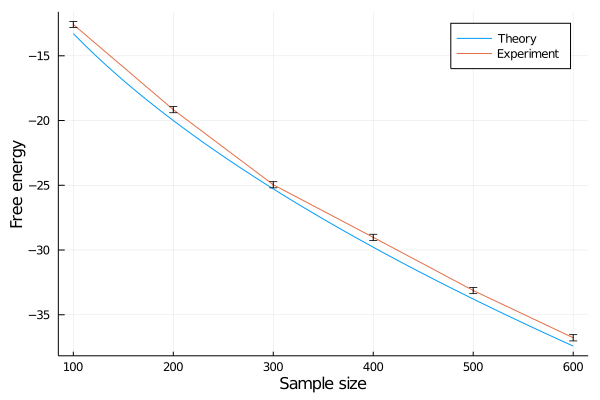
holds. In this case, eq. (45) gives the theoretical asymptotic behavior of the free energy versus inverse temperature for β=1\beta=1. Note that the KL-divergence between q(y,x) and p(y,x—a, b) in each neighborhood of the optimal parameter is regular, so λ=1​a​n​d​m=1\lambda=1andm=1. The expectation of the maximum value of a 2-dimensional Gaussian distribution follows a 1-dimensional Gaussian distribution (see the appendix). We will show that the theoretical behavior of free energy obeys

𝔼​[Fn​(1)]\displaystyle\mathbb{E}[F_{n}(1)] =n​L​(w0)−n​𝕍⁡[log⁡(p⁡(y|x,a0,b0))−log⁡(p⁡(y|x,−a0,b0))]2​π+log⁡n+O⁡(1).\displaystyle=nL(w_{0})-\sqrt{n}\sqrt{\frac{\mathbb{V}[\log(p(y|x,a_{0},b_{0}))-\log(p(y|x,-a_{0},b_{0}))]}{2\pi}}+\log n+O(1). (49)

In eq. (49), L⁡(w0)L(w_{0}) and the coefficient of n\sqrt{n} can be calculated by numerical integration. We used the average of FnF_{n} calculated from the true distribution q⁡(y|x),q⁡(x)q(y|x),q(x) as the experimental value of 𝔼⁡[Fn]\mathbb{E}[F_{n}]. The prior distribution p⁡(a)p(a), p⁡(b)p(b) does not have an effect on the asymptotic behavior. For this reason, we used equally spaced fixed values for integration. We compared this experimental values and theoretical values, except for the O⁡(1)O(1) term.

Refer to caption
Figure 1: Experimental value and theoretical free energy depending on the sample size. The error bar is the SE of the average of free energy. The theoretical value of log likelihood(n​L​(w0))(nL(w_{0})) is subtracted from each value.
Refer to caption
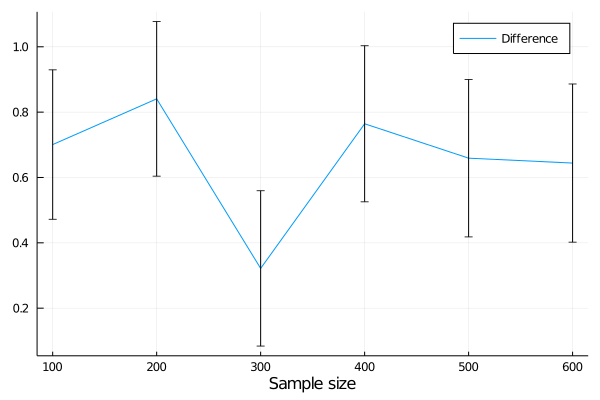
Figure 2: Difference between experimental value and theoretical value in Figure1. The error bar is the same as in Figure1.

We calculated the experimental values of 𝔼⁡[Fn]\mathbb{E}[F_{n}] whose sample sizes were n=100n=100 to 600600 every 100100. The number of samples ranged from 1000010000 to 6000060000 in steps of 1000010000 for each sample sizes. Figure1 compares the experimental and theoretical values. The experimental behavior of the free energy depending on the sample size is similar to the theoretical behavior. Figure2 shows the difference between the theoretical value and experimental value. This difference corresponds to O⁡(1)O(1) term. This difference is remains on this order regardless of the sample size. The experimental results support the theoretical formula, eq.(45).

6 Discussion

We found that if the optimal probability distribution is not unique, the apparent bias or the variance gets smaller for a finite sample number nn corresponding to a Gaussian process determined by the log loss of the optimal parameter set and the reduction converges to 0 asymptotically.This behavior can be explained qualitatively as follows: when there are two or more optimal probability distributions, the posterior distribution can be selected to be the nearest optimal probability distribution by bias of data, and this makes the generalization loss smaller than the average generation of data. As the number of samples and the bias increase, data generates averagely and generalization loss gets larger.
In this paper, we showed that the asymptotic behavior of the free energy and generalization loss are determined by n12n^{\frac{1}{2}} and n−12n^{-\frac{1}{2}} order. Previous research[13] provides concrete example in which there is a unique optimal probability distribution but assumption(8) does not hold. In that paper, the asymptotic behavior of the free energy and the generalization loss are determined by n13n^{\frac{1}{3}} and n−23n^{-\frac{2}{3}} order, so we predict that the lowest order determining the asymptotic behavior of the free energy and generalization loss are n12n^{\frac{1}{2}} and n−12n^{-\frac{1}{2}}.
We showed that the asymptotic behaviors of the free energy and generalization loss are determined by the maximum value of a Gauusian process. The probability distribution of the maximum value of a Gaussian process or multivariate normal distribution can not be calculated analytically, but an approximate calculation, called the “tube method”[4] exists. There is also a a method for calculating the upper and lower bounds of the expectation of the maximum value of a Gauusian process, called “chaining”[6].This maximum value is what determines the free energy and generalization loss in this paper.

7 Conclusion

We examined the case of when an important assumption in singular learning theory about the log density ration function is loosened. In this case there is a new term that is determined by a Gaussian process, whereby the generalization loss asymptotically increases as the size of the dataset increase. In the future, we should examine the asymptotic behavior of the generalization loss as a random variable, in particular the asymptotic equivalence of WAIC [12] and WBIC [14] in this case, and in the case in which the assumption is completely removed.

Appendix

We will derive the following equation.

𝔼⁡[max​ℒ​(w0)]=𝕍⁡[log⁡(p⁡(x|w01))−log⁡(p⁡(x|w02))]2​π\displaystyle\mathbb{E}[{\mbox{max}}\mathscr{L}(w_{0})]=\sqrt{\frac{\mathbb{V}[\log(p(x|w_{01}))-\log(p(x|w_{02}))]}{2\pi}} (A1)

In this equation, ℒ⁡(w0)\mathscr{L}(w_{0}) is a 2-dimensional gaussian distribution which average is 00 and variance-covariance matrix is

Vi​j=𝔼⁡[(log⁡p⁡(x|w0​i)+L⁡(w0))​(log⁡p⁡(x|w0​j)+L⁡(w0))]\displaystyle V_{ij}=\mathbb{E}[(\log p(x|w_{0i})+L(w_{0}))(\log p(x|w_{0j})+L(w_{0}))] (A2)

We define two random variables as

z1=ℒ⁡(w01)−ℒ⁡(w02).\displaystyle z_{1}=\mathscr{L}(w_{01})-\mathscr{L}(w_{02}).
z2=ℒ⁡(w01)+ℒ⁡(w02)\displaystyle z_{2}=\mathscr{L}(w_{01})+\mathscr{L}(w_{02})

The random variables (z1,z2)(z_{1},z_{2}) are also from 2-dimensional Gaussian distribution whose average is 00 and variance-covariance matrix is

(1−111)​(V11V12V21V22)\displaystyle\left(\begin{array}[]{ccc}1&-1\\ 1&1\end{array}\right)\left(\begin{array}[]{ccc}V_{11}&V_{12}\\ V_{21}&V_{22}\end{array}\right) (11−11)\displaystyle\left(\begin{array}[]{ccc}1&1\\ -1&1\end{array}\right)
=(V11+V22−V12−V21V11−V22+V12−V21V11−V22−V12+V21V11+V22+V12+V21).\displaystyle=\left(\begin{array}[]{ccc}V_{11}+V_{22}-V_{12}-V_{21}&V_{11}-V_{22}+V_{12}-V_{21}\\ V_{11}-V_{22}-V_{12}+V_{21}&V_{11}+V_{22}+V_{12}+V_{21}\end{array}\right).

The marginal distribution about z1z_{1} is a 1-dimensional Gaussian distribution whose average is 00 and the variance is

V11+V22−V12−V21.\displaystyle V_{11}+V_{22}-V_{12}-V_{21}.

According to eq.(16) and eq.(34), we have

V11\displaystyle V_{11} +V22−V12−V21\displaystyle+V_{22}-V_{12}-V_{21}
=𝔼[(logp(x|w01)(logp(x|w01)]−L(w0)2+𝔼[(logp(x|w02)(logp(x|w02)]\displaystyle=\mathbb{E}[(\log p(x|w_{01})(\log p(x|w_{01})]-L(w_{0})^{2}+\mathbb{E}[(\log p(x|w_{02})(\log p(x|w_{02})]
−L(w0)2−2(𝔼[(logp(x|w01)(logp(x|w02)]−L(w0)2)\displaystyle\qquad\qquad-L(w_{0})^{2}-2(\mathbb{E}[(\log p(x|w_{01})(\log p(x|w_{02})]-L(w_{0})^{2})
=𝔼⁡[(log⁡p⁡(x|w01)−log⁡p⁡(x|w02))2]\displaystyle=\mathbb{E}[(\log p(x|w_{01})-\log p(x|w_{02}))^{2}]
=𝕍⁡[(log⁡p⁡(x|w01)−log⁡p⁡(x|w02))]\displaystyle=\mathbb{V}[(\log p(x|w_{01})-\log p(x|w_{02}))] (A3)

We define a random variable z3z_{3}

z3={z1z1≥00z1<0\displaystyle z_{3}=\begin{cases}z_{1}&z_{1}\geq 0\\ 0&z_{1}<0\end{cases}

By using z3z_{3} we can describe the maximum value of ℒ⁡(w0)\mathscr{L}(w_{0}) in the following way,

max​ℒ​(w0)=ℒ⁡(w02)+z3.\displaystyle{\mbox{max}}\mathscr{L}(w_{0})=\mathscr{L}(w_{02})+z_{3}. (A4)

Considering the average of ℒ⁡(w02)\mathscr{L}(w_{02}) is 00, we find that

𝔼⁡[max​ℒ​(w0)]=𝔼⁡[z3].\displaystyle\mathbb{E}[{\mbox{max}}\mathscr{L}(w_{0})]=\mathbb{E}[z_{3}]. (A5)

𝔼⁡[z3]\mathbb{E}[z_{3}] is the expectation of a positive value in a Gaussian distribution. This integration of a Gaussian whose variance is σ2\sigma^{2} can be calculated as

∫0∞x2​π​exp⁡(−x22​σ2)\displaystyle\int_{0}^{\infty}\frac{x}{\sqrt{2\pi}}\exp\left(-\frac{x^{2}}{2\sigma^{2}}\right) =[−σ2​π​exp⁡(−x22​σ2)]0∞\displaystyle=\left[-\frac{\sigma}{\sqrt{2\pi}}\exp\left(-\frac{x^{2}}{2\sigma^{2}}\right)\right]_{0}^{\infty}
=σ2​π.\displaystyle=\frac{\sigma}{\sqrt{2\pi}}. (A6)

From (A3), (A5), and(A6), we have

𝔼⁡[max​ℒ​(w0)]=𝔼⁡[z3]=𝕍⁡[log⁡(p⁡(x|w01))−log⁡(p⁡(x|w02))]2​π.\displaystyle\mathbb{E}[{\mbox{max}}\mathscr{L}(w_{0})]=\mathbb{E}[z_{3}]=\sqrt{\frac{\mathbb{V}[\log(p(x|w_{01}))-\log(p(x|w_{02}))]}{2\pi}}.

Therefore (A1) holds.

References

  • [1] Akaike, H. (1974). A new look at the statistical model identification. IEEE transactions on automatic control, 19(6), 716-723
  • [2] Akaike, H. (1998). Likelihood and the Bayes procedure. In Selected papers of Hirotugu Akaike (pp. 309-332). Springer, New York, NY.
  • [3] Amari, S. I. (1993). A universal theorem on learning curves. Neural networks, 6(2), 161-166.
  • [4] Kuriki, S., & Takemura, A. (2008). The tube method for the moment index in projection pursuit. Journal of statistical planning and inference, 138(9), 2749-2762.
  • [5] Levin, E., Tishby, N., & Solla, S. A. (1990) Statistical approach to learning and generalization in layered neural networks. Proceedings of the IEEE 78(10).1568 - 1574.
  • [6] Talagrand, M. (2014). Upper and lower bounds for stochastic processes: modern methods and classical problems (Vol. 60). Springer Science & Business Media.13-73.
  • [7] Van Der Vaart, A. W., & Wellner, J. A. (1996). Weak convergence. In Weak convergence and empirical processes (pp. 16-28). Springer, New York, NY.
  • [8] Schwarz, G. (1978). Estimating the dimension of a model. The annals of statistics, 6(2), 461-464.
  • [9] Spiegelhalter, D. J., Best, N. G., Carlin, B. P., & Van Der Linde, A. (2002). Bayesian measures of model complexity and fit. Journal of the royal statistical society: Series b (statistical methodology), 64(4), 583-639.
  • [10] Watanabe, S. (2001). Algebraic analysis for nonidentifiable learning machines. Neural Computation, 13(4), 899-933.
  • [11] Watanabe,S.(2009) Algebraic geometry and statistical learning theory. Cambridge University Press.
  • [12] Watanabe, S. (2010). Asymptotic equivalence of Bayes cross validation and widely applicable information criterion in singular learning theory. Journal of Machine Learning Research, 11(Dec), 3571-3594.
  • [13] Watanabe, S. (2010). Asymptotic learning curve and renormalizable condition in statistical learning theory. In Journal of Physics: Conference Series (Vol. 233, No. 1, p. 012014). IOP Publishing.
  • [14] Watanabe, S. (2013). A widely applicable Bayesian information criterion. Journal of Machine Learning Research, 14(Mar), 867-897.