Electronic transport in molecular junctions: The generalized Kadanoff–Baym ansatz with initial contact and correlations
Abstract
The generalized Kadanoff–Baym ansatz (GKBA) offers a computationally inexpensive approach to simulate out-of-equilibrium quantum systems within the framework of nonequilibrium Green’s functions. For finite systems the limitation of neglecting initial correlations in the conventional GKBA approach has recently been overcome [Phys. Rev. B 98, 115148 (2018)]. However, in the context of quantum transport the contacted nature of the initial state, i.e., a junction connected to bulk leads, requires a further extension of the GKBA approach. In this work, we lay down a GKBA scheme which includes initial correlations in a partition-free setting. In practice, this means that the equilibration of the initially correlated and contacted molecular junction can be separated from the real-time evolution. The information about the contacted initial state is included in the out-of-equilibrium calculation via explicit evaluation of the memory integral for the embedding self-energy, which can be performed without affecting the computational scaling with the simulation time and system size. We demonstrate the developed method in carbon-based molecular junctions, where we study the role of electron correlations in transient current signatures.
I Introduction
State-of-the-art electronic components are engineered from nanoscale building blocks with emerging quantum phenomena Keimer and Moore 2017; Tokura, Kawasaki, and Nagaosa 2017; Basov, Averitt, and Hsieh 2017; Ronzani et al. 2018; Kokkoniemi et al. 2020. These devices are not isolated but affected by a wide variety of environmental conditions and external perturbations such as temperature variations, structural defects, and chemical contamination on the samples. The device operation is typically ultrafast; there is no guarantee for an instant relaxation to a static configuration once the device is switched on. Emerging transient effects depend on, e.g., quantum dynamics and correlations Wijewardane and Ullrich 2005; Verdozzi, Stefanucci, and Almbladh 2006; Myöhänen et al. 2008; Uimonen et al. 2011; Myöhänen et al. 2012; Latini et al. 2014; Talarico, Maniscalco, and Lo Gullo 2019; Talarico, Maniscalco, and Gullo 2020; Tuovinen et al. 2020, system geometry and topology Khosravi et al. 2009; Vieira, Capelle, and Ullrich 2009; Perfetto, Stefanucci, and Cini 2010; Rocha et al. 2015; Wang et al. 2015; Tuovinen et al. 2019a; Ridley, Sentef, and Tuovinen 2019; Tuovinen et al. 2019b, and the response to external perturbations or thermal gradients Croy and Saalmann 2009; Kurth et al. 2010; Foieri and Arrachea 2010; Ness and Dash 2011; Arrachea et al. 2012; Eich, Di Ventra, and Vignale 2016; Tuovinen et al. 2016a; Tuovinen et al. 2016b; Covito et al. 2018a; Karlsson et al. 2018; Honeychurch and Kosov 2019; Kershaw and Kosov 2020; Boström et al. 2020. Recently, pump-probe spectroscopic methods have grown in number rapidly leading to the current field of ultrafast materials science with sub-picosecond temporal resolution being routinely achieved Prechtel et al. 2012; Cocker et al. 2013; Hunter et al. 2015; Rashidi et al. 2016; Cocker et al. 2016; Jelic et al. 2017; Chávez-Cervantes et al. 2019; McIver et al. 2020.
To address all this, a fully time-dependent quantum description including many-body correlations is necessary, as the individual components of the systems are operating on ultrafast time scales at the quantum level. The nonequilibrium Green’s function (NEGF) approach Baym and Kadanoff 1961; Kadanoff and Baym 1962; Keldysh 1965; Danielewicz 1984; Stefanucci and van Leeuwen 2013; Balzer and Bonitz 2013 is a natural choice: The dynamical information about the system, e.g. electric currents or the photoemission spectrum, is encoded into the NEGF. Accessing this information requires solving the equations of motion for the NEGF which is computationally expensive. However, this can be made computationally more tractable by reducing the two-time-nature of the NEGF into a single-time-description. This approach, the generalized Kadanoff–Baym ansatz (GKBA) Lipavský, Špička, and Velický 1986, is a well-established procedure, and it has been succesfully applied in, e.g. molecular junctions Galperin and Tretiak 2008; Ness and Dash 2011; Latini et al. 2014; Hopjan et al. 2018; Karlsson et al. 2018; Cosco et al. 2020, and spectroscopical setups for atomic Balzer, Hermanns, and Bonitz 2012; Perfetto et al. 2015; Covito et al. 2018a; Covito et al. 2018b, molecular Boström et al. 2018; Perfetto et al. 2018; Perfetto et al. 2019; Perfetto et al. 2020, and condensed matter systems Perfetto et al. 2016; Sangalli et al. 2018; Schüler, Budich, and Werner 2019; Murakami et al. 2020; Tuovinen et al. 2020; Schüler et al. 2020.
In the language of the Keldysh formalism Keldysh 1965; Danielewicz 1984; Stefanucci and van Leeuwen 2013, the GKBA approach concerns with real-time Green’s functions, namely the lesser and greater Keldysh component. A drawback in this approach is that the so-called mixed Keldysh components, with one of the time arguments imaginary and the other one real, are not included. The role of these mixed components is to relate the equilibrium (Matsubara) calculation to the out-of-equilibrium one, and therefore a consistent description of the initial correlations is troublesome. It has been shown to be possible to include the initial correlations in the GKBA approach as a separate calculation Semkat, Bonitz, and Kremp 2003; Karlsson et al. 2018; Hopjan and Verdozzi 2019; Bonitz et al. 2019 although it has been customary to use a noncorrelated initial state and build up correlations via a time evolution excluding external perturbations Rios et al. 2011; Hermanns, Balzer, and Bonitz 2012.
For transport setups also the initial contacting of the molecular junction contributes to the initial correlations. In the partitioned approach Caroli et al. 1971a; Caroli et al. 1971b the initial state is uncontacted, and the molecular region is suddenly brought into contact with the leads. In this case, the initial correlation collision integral due to the contact or embedding self-energy vanishes. The contacted initial state can be constructed by a sudden or adiabatic switching (AS) of the contacts and evolving the system without external fields to a contacted equilibrium. In the partition-free approach Cini 1980 the initial state is contacted, and there is a unique thermo-chemical equilibrium. The information about this coupled equilibrium is then encoded in the initial correlation (IC) collision integral . In this paper, we derive an expression for in closed form for the embedding self-energy. This calculation can be separated from the time-evolution, similar to Ref. Karlsson et al. 2018. The derived expression can directly be combined with many-body self-energies, resulting in a partition-free approach to the GKBA time-evolution for an initially correlated and contacted transport setup.
The paper is organized as follows. In Sec. II we introduce the model system and the governing equations of the GKBA approach (with the underlying NEGF theory detailed in Appendix A). We outline the calculation of the initial contacting collision integral in Sec. III and defer the implementation details to Appendix B and C. Then, in Sec. IV we present numerical simulations for time-resolved electronic transport in carbon-based molecular junctions. We draw our conclusions and discuss future prospects in Sec. V.
II Model and method
We consider an electronic junction consisting of a quantum-correlated molecular device () which is connected to an arbitrary number of noninteracting, metallic leads (), see Fig. 1. The molecular junction is described in terms of the second-quantized Hamiltonian
| (1) |
where label a complete set of single-electron states in the molecular device, and labels the leads. Above, describes the single-electron energy state in the -th lead, are the single-particle matrix elements for the molecular region, are the tunneling matrix elements between the molecular device and the leads, and are the two-electron Coulomb integrals for the molecular device. The annihilation (creation) operator removes (creates) an electron from (to) state with spin orientation , and they obey the fermionic anti-commutation rules for indices belonging either to the leads or to the molecular device.
We note that all objects introduced in Eq. (II) are diagonal in spin space. However, the following consideration could straightforwardly be extended to cases with, e.g., spin–orbit or Zeeman terms in the molecular Hamiltonian Tuovinen et al. 2019b, or ferromagnetic leads Krawiec and Wysokiński 2006. In addition, it would be possible to include a contribution from a thermomechanical field to the lead energy dispersion giving rise to a relative temperature shift in the leads Luttinger 1964; Eich et al. 2014; Eich, Di Ventra, and Vignale 2016; Covito et al. 2018c; Perfetto and Stefanucci 2018.
To access time-dependent nonequilibrium quantities for the system described by Eq. (II), we consider the equation of motion for the single-particle density matrix (see Appendix A for background)
| (2) |
where is the single-particle Hamiltonian supplemented with the time-local Hartree–Fock (HF) self-energy. The time-nonlocal self-energies due to many-particle and embedding effects appear in the collision integrals
| (3) | ||||
| (4) |
where marks the time when the system is driven out of equilibrium, and is the (equilibrium) inverse temperature. We refer to Appendix A for the description of the different components, e.g., the greater () and lesser () functions. Solving Eq. (2) is computationally demanding due to the full two-time history of the functions in Eqs. (3) and (4), and because of the self-energies’ functional dependency on the Green’s functions .
To reduce the computational complexity the Green’s functions are commonly approximated by the GKBA
| (5) |
with and , and the propagators are described for the coupled system at the HF level
| (6) |
where is the chronological time-ordering and is the tunneling probability matrix from the leads to the molecular region. Here we have used the wide-band approximation (WBA) for the retarded/advanced embedding self-energy, see Appendix B. This choice guarantees the same mathematical structure for the propagators as for the free-particle (or the HF) propagator, and it is expected to provide an accurate description when the retarded/advanced embedding self-energy depends weakly on frequency around the Fermi level. In contrast, the frequency dependence of the lesser/greater embedding self-energy can be included in Eq. (3), cf. Eq. (B).
While Eq. (2) in combination with Eq. (5) [and the self-energies in Eqs. (28), (A), and (26)] represents a closed set of equations, it only applies to the GKBA in the absence of initial contact and correlations, in Eq. (4). This is because the GKBA does not provide an approximation for the mixed functions in Eq. (4). It is possible to pass over this issue by starting the time-evolution from an initially noncorrelated state and then building up correlations by adiabatically switching on the many-particle and embedding effects Rios et al. 2011; Hermanns, Balzer, and Bonitz 2012. This procedure may, however, lead to unpractically long propagation times putting the computational gain of the GKBA in jeopardy compared to the full Kadanoff–Baym equations Karlsson et al. 2018; Tuovinen et al. 2019c; Tuovinen et al. 2020. However, the inclusion of the initial correlations has been shown to be possible also within GKBA Semkat, Bonitz, and Kremp 2003; Karlsson et al. 2018; Hopjan and Verdozzi 2019; Bonitz et al. 2019.
In Ref. Karlsson et al. 2018 a closed-form expression for in terms of was derived for a closed system where electron–electron interactions were described by the second-order Born self-energy. In the next section we will outline a similar procedure to evaluate for the embedding self-energy. This procedure can directly be combined with many-body self-energies, making it possible to perform GKBA time-evolution for an initially correlated and contacted transport setup. This constitutes a partition-free framework for electronic transport in terms of the GKBA.
III Initial contacting collision integral
Let us start by separating the collision integral in Eq. (4) for the correlation and contacting contributions as
| (7) |
For the first term (mb), we directly use the result derived in Ref. Karlsson et al. 2018 employing the second-order Born self-energy. For the second term (em), we take the self-energies as the embedding ones
| (8) |
The objects in Eq. (8) satisfy the same analytic structure as in Ref. Karlsson et al. 2018, enabling us to write a generalized fluctuation-dissipation theorem for the Green’s function and self-energy. This further allows for writing Eq. (8) equivalently in terms of the real-time lesser and greater functions Karlsson et al. 2018
| (9) |
where Eqs. (5) and (B) are to be employed for the Green’s functions and embedding self-energies, respectively. In general Eq. (9) involves a convergence factor in the integrand (see Ref. Karlsson et al. 2018). However, with contacted infinite leads this factor can be left out as the embedding self-energy accounts for proper convergence due to presence of a continuum of lead states. We notice that for we have , i.e., the retareded Green function, , vanishes whereas the advanced Green function, , does not [cf. Eq. (6)]. Importantly, for times , the single-particle density matrix is static, given by some equilibrium value, . In this time interval, the HF Hamiltonian also becomes static, . These time intervals may then be separated using the group property
| (10) |
Note that here the equilibrium system is taken as coupled, and appearing in the exponent is due to the WBA, in accordance with Eq. (6).
With these considerations Eq. (9) can be expanded as
| (11) |
Here, it is worth noting that the frequency-dependence of results from the lesser/greater embedding self-energy in Eq. (B), which itself is of general form and does not require the WBA. For the system is in equilibrium, i.e., external fields are not switched on. For the bias voltage phase factor we therefore have . Then, by canceling and combining some terms we may isolate the integration
| (12) |
The time integration is now straightforward to perform and we are left with a frequency integral only. This gives us as the final result for the initial contacting collision integral
| (13) |
where we used the notation and for a scalar and a matrix .
Importantly, we are left with no time integrations, so Eq. (13) can be evaluated at any time with minor computational cost, provided that is already available during the time evolution. We discuss in Appendix C the case of taking explicitly the WBA for Eq. (13), which lightens the computational cost even more. If, in addition, we consider a specific but frequently used harmonic bias voltage profile, , also the phase factor can be expanded in terms of Bessel functions Jauho, Wingreen, and Meir 1994; Ridley, MacKinnon, and Kantorovich 2015; Ridley and Tuovinen 2017.
The time-dependent current between the molecular region and the leads can be calculated by the Meir–Wingreen formula Meir and Wingreen 1992; Jauho, Wingreen, and Meir 1994
| (14) |
This needs to be adjusted to include the effect from the initial contacting collision integral in Eq. (13). The adjustment can be obtained by writing Eq. (13) as , and then identifying the time-dependent current as
| (15) |
We note that a corresponding contribution arising from the many-body self-energy vanishes due to conservation laws and the self-consistent solution to the equations of motion Talarico, Maniscalco, and Lo Gullo 2019.
IV Results
We now demonstrate the protocol derived in the previous section. In all of the numerical simulations presented we consider two separate cases: (1) the standard GKBA time evolution where the correlated and contacted initial state is prepared by an adiabatic switching procedure for and then switching on the bias voltage at ; and (2) the GKBA time evolution supplemented with the initial correlations and contacting collision integral, starting the simulation directly at with the bias voltage. We refer to the former case as ‘GKBAAS’ and to the latter as ‘GKBAIC’. As we wish to analyze the validity of the initial contacting protocol, we consider the electronic interactions at the HF and 2B level. Note that in the HF case in Eq. (7), and in the 2B case this contribution is evaluated using the approach of Ref. Karlsson et al. 2018.
We consider two different molecular junctions where the ‘molecule’ being coupled to macroscopic metallic leads is (i) cyclobutadiene and (ii) a graphene nanoflake. The modeling for the molecular regions is done at the Pariser–Parr–Pople Pariser and Parr 1953; Pople 1953 (PPP) level, where the kinetic and interaction matrix elements are obtained semi-empirically by fitting to more sophisticated calculations.
The macroscopic metallic leads are described as noninteracting semi-infinite tight-binding lattices. The role of the leads is to act as particle reservoirs and as biased electrodes accounting for a potential drop across the molecular region. The potential drop is modeled by a symmetric bias voltage , see Appendix A. We also consider the zero-temperature limit at which we derive in Appendix B a fast and accurate analytical representation of the embedding self-energy in terms of Bessel and Struve functions. The matrix structure of the embedding self-energy is specified by the coupling matrix elements between the molecular region and the leads: In all of the cases considered the left-most atoms of the molecular region are coupled to the left lead, and the right-most atoms of the molecular region are coupled to the right lead with equal coupling strength where . The energy scale in the lead is specified by the hopping strength between the lead sites .
IV.1 Cyclobutadiene
We consider a cyclobutadiene molecule attached to donor–acceptor-like leads. This is a circular molecule of atomic sites, and it is modeled by PPP parameters obtained by fitting to an effective valence shell Hamiltonian method Martin and Freed 1996. The single-particle matrix is taken as (in atomic units)
| (16) |
and the two-body interaction is of the form with (in atomic units)
| (17) |
Note the slightly asymmetric structure of the hopping and interaction matrix elements due to cyclobutadiene being a rectangle, not a square Breslow and Foss Jr 2008. The coupling between the molecule and the leads is of equal strength a.u. from the molecular sites and to the left lead and from the molecular sites and to the right lead. The hopping energy in the leads is a.u., which gives for the tunneling rate a.u. The chemical potential is set between the highest occupied molecular orbital (HOMO) and the lowest unoccupied molecular orbital (LUMO), a.u., of the isolated molecule with two electrons. Such simplified modeling of the molecular junction enables us to address the new approach with mathematical transparency, also comparing the GKBA with the full Kadanoff–Baym equation (KBE) approach of Ref. Myöhänen et al. 2009.
In Fig. 2 we show the time-dependent densities (at the first site) and currents (through the left lead interface) in the cyclobutadiene molecular junction. We see that the restart protocol of GKBA with the initial contacting (GKBAIC) is very well in agreement with the adiabatic switching (GKBAAS) for both the density and the current, and for both weak and strong bias. In addition, we have checked (not shown) that in the absence of bias the GKBAIC time evolution remains stable and unchanged from the state described by . Even though the bias window in the strong-bias case extends up to half the bandwidth, we still observe a satisfactory agreement between GKBA and KBE at the HF level. At the 2B level compared to full KBE, we find a typical mismatch of the steady-state density and current. This can be addressed in terms of the out-of-equilibrium spectral function, which is calculated as a Fourier transformation with respect to the relative-time coordinate :
| (18) |
where we set the center-of-time coordinate, , to half the total propagation time, so that the relative-time coordinate spans the maximal range diagonally in the two-time plane. In Fig. 3 we show the energy diagram together with the out-of-equilibrium spectral functions. As the GKBA in Eq. (5) satisfies the exact condition , the GKBA spectral function adheres to the form of the HF propagators in Eq. (6). This is generally in agreement with Refs. Thygesen 2008; Myöhänen et al. 2009 for similar systems. Here the interaction is relatively strong, so the KBE 2B spectral function is completely smeared out.
IV.2 Graphene nanoflake
We then consider a graphene nanoflake which has more structural complexity, see Fig. 4. The molecular region is a notched armchair graphene nanoribbon of width and length similar to Ref. Hancock et al. 2010 where a generalized tight-binding model was proposed. It was found that a single parameter set with first-, second-, and third-nearest neighbor hoppings eV, eV, eV, and a Hubbard interaction eV accurately reproduced density-functional theory based results for both the band structure and the conductance. We choose these values as the PPP parameters along the hexagonal lattice in Fig. 4 for Eq. (II): for first-, second-, and third-nearest neighbors, respectively, and . Here we describe the interactions at the 2B level. We note that, as we include next-nearest neighbor hoppings, the electron-hole symmetry is not preserved Castro Neto et al. 2009. In addition, the nanoflake is coupled to the left and right leads from the left-most and right-most carbon atoms, respectively (see Fig. 4). We consider two cases of tunneling rates between the graphene nanoflake and the leads , and we fix the bias voltage to with respect to the chemical potential eV, which is set in the middle of the HOMO–LUMO gap of the isolated graphene nanoflake. As the energies are in electronvolts, eV, we convert the units for time to seconds by s, and the units for current to amperes by A.

The restart protocol with the initial contacting (GKBAIC) relies on a converged initial state. In Fig. 5 we show the time-dependent currents (through the left lead interface) for the graphene nanoflake molecular junction, and we study the role of the switching time and the tunneling rate . First, the initial contacting (GKBAIC) is in excellent agreement with the adiabatic switching (GKBAAS) for both weak and intermediate coupling. Second, the relaxation time of the switching procedure is longer for weaker coupling Latini et al. 2014. This is reflected on the initial contacting protocol, which requires an equilibrium density matrix as input. If this does not result from a properly converged calculation, then GKBAIC starts deviating from GKBAAS, as can be seen in Fig. 5 cases fs and fs. We emphasize that the computational cost for the GKBAIC is independent on how long the preparation stage takes: With one prepared , as many out-of-equilibrium simulations as desired may be performed (e.g. voltage sweep).
In Fig. 5 we also show a simulation with the HF self-energy: Compared to the 2B case, the transient oscillation is roughly similar and only the steady-state value is affected within the GKBA description. For this size of the graphene structure and this model of interaction, this is reasonable as monolayer graphene devices are known to have fairly large coherent transport lengths Castro Neto et al. 2009. In Fig. 5 we also show, for comparison, an ill-advised simulation of a simultaneous and sudden switch-on of both many-body correlations and contacts with voltage at . Clearly, the transient features are completely misrepresented in this case, but the long-time limit coincides with the AS and IC results due to loss of memory of the initial state Stefanucci and Almbladh 2004. Generally, with the chosen parameters for voltage and coupling, we find the absolute values of the stationary currents in the mA range, and the transient signature characterized in the fs temporal range.
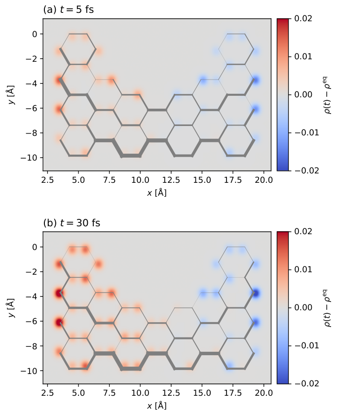
The dominant transient oscillation observed in Fig. 5 is independent of the tunneling rate and corresponds to a frequency of which is equal to the applied bias voltage. Therefore, these oscillations represent transitions between the biased Fermi level of the leads and the zero-energy states of the graphene nanoflake Tuovinen et al. 2013; Tuovinen et al. 2014. These zero-energy states correspond to surface states along the zigzag segments of the graphene nanoflake Fujita et al. 1996; Tao et al. 2011. This is confirmed in Fig. 6 where the excited zero-energy modes are spatially focused along the surface during the initial transient. Interestingly, this effect therefore seems to be robust against electronic interactions. While it is outside of the scope of the present work, this effect could be associated with nontrivial spin polarization or antiferromagnetic alignment at the edges of the system Yamashiro et al. 2003; Fernández-Rossier 2008; Lado, García-Martínez, and Fernández-Rossier 2015. As the system relaxes towards the stationary state, the density response becomes more delocalized along the nanoflake. In Fig. 6 we also show the relative strength of the bond current between nearest-neighbor carbon atoms. Due to the notched geometry, the current is appreciably stronger in the lower part of the nanoflake. We suspect larger graphene nanostructures would show even more pronounced separation of the charge and current density between the bulk and the surface during the initial transient Rocha et al. 2015.
V Conclusion
We have extended the GKBA approach for open quantum systems to a partition-free setting in electronic transport. We formulated the initial state for a molecular junction, before applying, e.g., a bias voltage driving, as correlated and contacted. In practice, the contacted initial state was resolved as a separate calculation, which could be included to the out-of-equilibrium calculation via the initial contacting collision integral with a minor computational cost. This approach could directly be combined with the initial correlations in Ref. Karlsson et al. 2018, making it possible to perform GKBA time-evolution for an initially correlated and contacted transport setup.
The inclusion of the initial contacting collision integral is very general. Since it only concerns the embedding self-energy, extensions to more sophisticated correlation self-energies, such as the -matrix Galitskii 1958 or the approximation Hedin 1965, are directly applicable. In addition, extensions to correlated approximations to the propagators are applicable as long as they can be represented by , where includes some quasiparticle effects Latini et al. 2014; Perfetto and Stefanucci 2018. Even though we only considered constant bias voltage profiles, the driving could also be modulated in time Jauho, Wingreen, and Meir 1994; Ridley, MacKinnon, and Kantorovich 2015; Ridley and Tuovinen 2017.
We demonstrated the developed method by studying transient current signatures in carbon-based molecular junctions. A compact system of a cyclobutadiene molecule allowed for a transparent comparison of the new approach to adiabatic switching GKBA, and even to the full Kadanoff–Baym equation. Time-resolved densities and currents via the initial contacting approach were found to be in excellent agreement with the adiabatic switching approach in both weak- and strong-bias regimes. A more structurally complex system of a graphene nanoflake addressed both the potential and the limitations of the new approach. While the comparison with the adiabatic switching approach was found to be successful, it was important to verify the convergence of the initially correlated and contacted state before initiating an out-of-equilibrium simulation. We also found predominant oscillations in the transient current signal associated with virtual transitions between the graphene surface states and the biased Fermi levels of the lead. Together with recent experimental developments in ultrafast techniques these findings highlight the potential of addressing transiently emerging topological phenomena in molecular junctions out of equilibrium.
Acknowledgements.
This research was funded by the Academy of Finland projects 321540 (R.T.) and 317139 (R.v.L.). G.S. and E.P. acknowledge financial support from MIUR PRIN Grant No. 20173B72NB, from INFN through the TIME2QUEST project and from Tor Vergata University through the Beyond Borders Project ULEXIEX. The computer resources of the Finnish IT Center for Science (CSC) and the FGCI project (Finland) are acknowledged. R.T. also acknowledges useful discussions with N. W. Talarico, F. Cosco, and N. Lo Gullo.Data availability
The data that support the findings of this study are available from the corresponding author upon reasonable request.
Appendix A Background for the NEGF-GKBA equations
Generally, the Hamiltonian in Eq. (II) is described with an argument referring to a time parameter on the Konstantinov–Perel’ time contour Konstantinov and Perel’ 1961 , where marks the beginning of a transport process generated by, e.g., a voltage switch-on, is the observation time, and is the inverse temperature. The molecular junction Hamiltonian may then be specified for all contour times as Ridley and Tuovinen 2018
| (19) | ||||
| (20) |
where we introduced a bias voltage profile for the lead energy dispersion, a nonlocal potential profile for the molecular device, and the equilibrium chemical potential . The coupling and interaction matrix elements can either be set equal and nonzero for all , or zero for and proportional to a switching function for on the horizontal branches.
The one-electron Green’s function is defined on the time contour as Stefanucci and van Leeuwen 2013
| (21) |
where is the contour-time-ordering, the creation and annihilation operators are represented in the Heisenberg picture, and the ensemble average is taken as a trace over the density matrix. The Green’s function satisfies the equation of motion (in matrix form) Stefanucci and van Leeuwen 2013
| (22) |
and the corresponding adjoint equation. In Eq. (22) we introduced a block matrix structure with respect to the basis of single-electron states
| (23) |
where the lead part is diagonal, , the tunneling is through the molecular device, , and . In Eq. (22) we also wrote the many-body self-energy accounting for the electronic interactions. While this interaction is constricted to the molecular region only, the Green’s function matrix has nonzero entries everywhere:
| (24) |
The integration in Eq. (22) is performed over the Konstantinov–Perel’ contour through the Langreth rules Langreth and Wilkins 1972; Langreth 1976. In this procedure, the contour-time functions are represented in real-time components: lesser (), greater (), retarded (R), advanced (A), left (), right (), and Matsubara (M) depending on the contour-time arguments Stefanucci and van Leeuwen 2013.
We now consider the molecular region and take the projection of the equation of motion (22) onto these states. This procedure leads to Myöhänen et al. 2009
| (25) |
and a similar adjoint equation. In Eq. (A) we defined the embedding self-energy as
| (26) |
where the Green’s function of the noninteracting lead satisfies . As we are mainly considering the dynamical quantities within the molecular region, we will drop the subscript for simplicity.
We consider the electronic interaction at the Hartree–Fock (HF) and second-order Born (2B) level, which are time-local and time-nonlocal, respectively
| (27) |
This separation allows us to remove the time-local part from the collision integral on the right-hand side of Eq. (A), and couple it with the single-particle Hamiltonian on the left-hand side. Using the basis of single-electron states, the HF self-energy reads
| (28) |
where is the single-particle density matrix. The 2B self-energy takes the form
| (29) |
where the summation over the basis states can be reorganized for efficient computation Perfetto and Stefanucci 2019; Schlünzen et al. 2019; Tuovinen, Covito, and Sentef 2019.
Appendix B Embedding self-energy
Since the leads are treated as noninteracting, they can be incorporated non-perturbatively into the equation of motion (A) using the embedding self-energy in Eq. (26). On the real-time branch the relevant lead Green’s functions are Stefanucci and van Leeuwen 2013
| (30) | ||||
| (31) |
where is the Fermi function at inverse temperature with the property . The retarded and advanced embedding self-energies are then given by Ridley, MacKinnon, and Kantorovich 2015
| (32) |
where is the phase factor originating from the bias voltage profile, and we wrote the level-shift and level-width matrices as
| (33) | ||||
| (34) |
respectively. In Eqs. (33) and (34) we used with being a positive infinitesimal and denoting the principal value.
In the wide-band approximation (WBA) the level-width is taken as independent of frequency, . This amounts to approximating the lead density of states being practically featureless in the energy scale of the molecular system. In this approximation the level-shift matrix vanishes due to Kramers–Kronig relations, and the retarded/advanced embedding self-energy becomes time-local
| (35) |
In a similar manner we obtain the lesser/greater embedding self-energy as Croy and Saalmann 2009
| (36) |
Even though we set ourselves in the regime where the WBA holds, in Eq. (B) we keep the frequency dependency of to ensure convergence of the frequency integral.
The matrix structure of the embedding self-energy is determined by the corresponding structure of the level-width matrix which is specified by the coupling and lead Hamiltonians in Eq. (34). We now address the frequency integral in Eq. (B) and consider the effective form of the level-width matrix for a one-dimensional semi-infinite tight-binding lead Myöhänen et al. 2009
| (37) |
where is the on-site energy of the sites in lead and the hopping energy between the sites in lead . This form also limits the integration range to , see Fig. 3(a). We also consider the zero-temperature limit at which the Fermi function becomes a Heaviside step function, , and this introduces a further cutoff to the integral. We also write for brevity and obtain
| (38) |
We make the identification that the on-site energies in the leads are aligned with the equilibrium chemical potential, , resulting in half filling for the leads’ energy continua. Making a change of variables we obtain
| (39) |
where on the last line we used an integral representation of the Bessel and Struve functions of the first kind DLMF; Zhu et al. 2005. We remind that the final result for the lesser embedding self-energy at the zero-temperature limit, obtained by inserting Eq. (B) in Eq. (B), needs to be supplemented with the appropriate matrix structure. We also note that at the equal-time limit, , Eq. (B) reduces to a value of . The case of the greater embedding self-energy with in Eq. (B) results in the integral which has otherwise the same representation as in Eq. (B) but the sign in front of the Struve function is changed. The Struve function can be evaluated using an approximate expansion in terms of the Bessel functions Aarts and Janssen 2003; Aarts and Janssen 2016, or as a direct combination of power series and continued fraction Zhang and Jin 1996.
Appendix C Evaluation of the frequency integral at the wide-band approximation
In practice, we evaluated Eq. (13) by numerical integration for all the simulations presented. However, we can make some further analytical progress by taking explictly the WBA. We show here how, in this case, the frequency integral in Eq. (13) can further be expressed in terms of the hypergeometric function DLMF which can be evaluated using a fast and accurate numerical algorithm Michel and Stoitsov 2008. Now, due to the lesser/greater embedding self-energy is also taken as independent of frequency, and Eq. (13) can be written as
| (40) |
Here we used the fact that the frequency integral is performed over the full real axis , and it can be evaluated using contour integration techniques. The exponential factor in the numerator converges only in the lower-half of the complex plane. In this region the contribution from Eq. (13) does not contain any poles, so this contribution to the integral vanishes. The other contribution contains the Matsubara poles of the Fermi function, in the lower-half of the complex plane, keeping the integral nonzero.
We may then expand the result in the (right) eigenvector basis of the nonhermitian matrix
| (41) |
We recall that the left/right eigenvectors of a nonhermitian matrix form a biorthogonal basis set. The frequency integral of Eq. (40) in this basis reads
| (42) |
Due to the exponential factor in the numerator, we close the integration contour in the lower-half plane. Since is an eigenvalue of , it is located on the upper-half plane ( is a positive-definite matrix). Then, in the lower-half plane, only the residues at the Matsubara poles, (with integer), contribute to the integral. This consideration is very similar to Ref. Tuovinen et al. 2019b, and also here it is possible to show that the result can be written in terms of the hypergeometric function DLMF
| (43) |
After this manipulation, Eq. (C) can simply be inserted back into Eq. (40) with a suitable rotation of the left/right eigenvectors Tuovinen et al. 2019b.
While, in this approach, the restart protocol (GKBAIC) is consistent with the adiabatic switching (GKBAAS) only when the WBA is a good approximation, this is still a fairly practical way of computing the initial contacting collision integral in Eq. (13) because it is considerably faster than numerical integration and can be performed to arbitrary numerical precision Michel and Stoitsov 2008. In addition, the GKBA approach is expected to be accurate in this regime due to the choice of propagators at the level of WBA. We have checked that the transient features presented in Figs. 2 and 5 are very well represented also when using Eq. (40) with Eq. (C).
References
- Keimer and Moore (2017) B. Keimer and J. E. Moore, Nat. Phys. 13, 1045 (2017).
- Tokura, Kawasaki, and Nagaosa (2017) Y. Tokura, M. Kawasaki, and N. Nagaosa, Nat. Phys. 13, 1056 (2017).
- Basov, Averitt, and Hsieh (2017) D. N. Basov, R. D. Averitt, and D. Hsieh, Nat. Mater. 16, 1077 (2017).
- Ronzani et al. (2018) A. Ronzani, B. Karimi, J. Senior, Y.-C. Chang, J. T. Peltonen, C. Chen, and J. P. Pekola, Nat. Phys. 14, 991 (2018).
- Kokkoniemi et al. (2020) R. Kokkoniemi, J.-P. Girard, D. Hazra, A. Laitinen, J. Govenius, R. E. Lake, I. Sallinen, V. Vesterinen, M. Partanen, J. Y. Tan, K. W. Chan, K. Y. Tan, P. Hakonen, and M. Möttönen, Nature 586, 47 (2020).
- Wijewardane and Ullrich (2005) H. O. Wijewardane and C. A. Ullrich, Phys. Rev. Lett. 95, 086401 (2005).
- Verdozzi, Stefanucci, and Almbladh (2006) C. Verdozzi, G. Stefanucci, and C.-O. Almbladh, Phys. Rev. Lett. 97, 046603 (2006).
- Myöhänen et al. (2008) P. Myöhänen, A. Stan, G. Stefanucci, and R. van Leeuwen, EPL 84, 67001 (2008).
- Uimonen et al. (2011) A.-M. Uimonen, E. Khosravi, A. Stan, G. Stefanucci, S. Kurth, R. van Leeuwen, and E. K. U. Gross, Phys. Rev. B 84, 115103 (2011).
- Myöhänen et al. (2012) P. Myöhänen, R. Tuovinen, T. Korhonen, G. Stefanucci, and R. van Leeuwen, Phys. Rev. B 85, 075105 (2012).
- Latini et al. (2014) S. Latini, E. Perfetto, A.-M. Uimonen, R. van Leeuwen, and G. Stefanucci, Phys. Rev. B 89, 075306 (2014).
- Talarico, Maniscalco, and Lo Gullo (2019) N. W. Talarico, S. Maniscalco, and N. Lo Gullo, Phys. Status Solidi B 256, 1800501 (2019).
- Talarico, Maniscalco, and Gullo (2020) N. W. Talarico, S. Maniscalco, and N. L. Gullo, Phys. Rev. B 101, 045103 (2020).
- Tuovinen et al. (2020) R. Tuovinen, D. Golež, M. Eckstein, and M. A. Sentef, Phys. Rev. B 102, 115157 (2020).
- Khosravi et al. (2009) E. Khosravi, G. Stefanucci, S. Kurth, and E. K. U. Gross, Phys. Chem. Chem. Phys. 11, 4535 (2009).
- Vieira, Capelle, and Ullrich (2009) D. Vieira, K. Capelle, and C. A. Ullrich, Phys. Chem. Chem. Phys. 11, 4647 (2009).
- Perfetto, Stefanucci, and Cini (2010) E. Perfetto, G. Stefanucci, and M. Cini, Phys. Rev. B 82, 035446 (2010).
- Rocha et al. (2015) C. G. Rocha, R. Tuovinen, R. van Leeuwen, and P. Koskinen, Nanoscale 7, 8627 (2015).
- Wang et al. (2015) B. Wang, J. Li, F. Xu, Y. Wei, J. Wang, and H. Guo, Nanoscale 7, 10030 (2015).
- Tuovinen et al. (2019a) R. Tuovinen, M. A. Sentef, C. Gomes da Rocha, and M. S. Ferreira, Nanoscale 11, 12296 (2019a).
- Ridley, Sentef, and Tuovinen (2019) M. Ridley, M. A. Sentef, and R. Tuovinen, Entropy 21, 737 (2019).
- Tuovinen et al. (2019b) R. Tuovinen, E. Perfetto, R. van Leeuwen, G. Stefanucci, and M. A. Sentef, New J. Phys. 21, 103038 (2019b).
- Croy and Saalmann (2009) A. Croy and U. Saalmann, Phys. Rev. B 80, 245311 (2009).
- Kurth et al. (2010) S. Kurth, G. Stefanucci, E. Khosravi, C. Verdozzi, and E. K. U. Gross, Phys. Rev. Lett. 104, 236801 (2010).
- Foieri and Arrachea (2010) F. Foieri and L. Arrachea, Phys. Rev. B 82, 125434 (2010).
- Ness and Dash (2011) H. Ness and L. K. Dash, Phys. Rev. B 84, 235428 (2011).
- Arrachea et al. (2012) L. Arrachea, E. R. Mucciolo, C. Chamon, and R. B. Capaz, Phys. Rev. B 86, 125424 (2012).
- Eich, Di Ventra, and Vignale (2016) F. G. Eich, M. Di Ventra, and G. Vignale, Phys. Rev. B 93, 134309 (2016).
- Tuovinen et al. (2016a) R. Tuovinen, R. van Leeuwen, E. Perfetto, and G. Stefanucci, J. Phys. Conf. Ser. 696, 012016 (2016a).
- Tuovinen et al. (2016b) R. Tuovinen, N. Säkkinen, D. Karlsson, G. Stefanucci, and R. van Leeuwen, Phys. Rev. B 93, 214301 (2016b).
- Covito et al. (2018a) F. Covito, E. Perfetto, A. Rubio, and G. Stefanucci, Eur. Phys. J. B 91, 216 (2018a).
- Karlsson et al. (2018) D. Karlsson, R. van Leeuwen, E. Perfetto, and G. Stefanucci, Phys. Rev. B 98, 115148 (2018).
- Honeychurch and Kosov (2019) T. D. Honeychurch and D. S. Kosov, Phys. Rev. B 100, 245423 (2019).
- Kershaw and Kosov (2020) V. F. Kershaw and D. S. Kosov, J. Chem. Phys. 153, 154101 (2020).
- Boström et al. (2020) E. V. Boström, M. Claassen, J. W. McIver, G. Jotzu, A. Rubio, and M. A. Sentef, SciPost Phys. 9, 61 (2020).
- Prechtel et al. (2012) L. Prechtel, L. Song, D. Schuh, P. Ajayan, W. Wegscheider, and A. W. Holleitner, Nat. Commun. 3, 646 (2012).
- Cocker et al. (2013) T. L. Cocker, V. Jelic, M. Gupta, S. J. Molesky, J. A. J. Burgess, G. D. L. Reyes, L. V. Titova, Y. Y. Tsui, M. R. Freeman, and F. A. Hegmann, Nat. Photonics 7, 620 (2013).
- Hunter et al. (2015) N. Hunter, A. S. Mayorov, C. D. Wood, C. Russell, L. Li, E. H. Linfield, A. G. Davies, and J. E. Cunningham, Nano Lett. 15, 1591 (2015).
- Rashidi et al. (2016) M. Rashidi, J. A. J. Burgess, M. Taucer, R. Achal, J. L. Pitters, S. Loth, and R. A. Wolkow, Nat. Commun. 7, 13258 (2016).
- Cocker et al. (2016) T. L. Cocker, D. Peller, P. Yu, J. Repp, and R. Huber, Nature 539, 263 (2016).
- Jelic et al. (2017) V. Jelic, K. Iwaszczuk, P. H. Nguyen, C. Rathje, G. J. Hornig, H. M. Sharum, J. R. Hoffman, M. R. Freeman, and F. A. Hegmann, Nat. Phys. 13, 591 (2017).
- Chávez-Cervantes et al. (2019) M. Chávez-Cervantes, G. E. Topp, S. Aeschlimann, R. Krause, S. A. Sato, M. A. Sentef, and I. Gierz, Phys. Rev. Lett. 123, 036405 (2019).
- McIver et al. (2020) J. W. McIver, B. Schulte, F.-U. Stein, T. Matsuyama, G. Jotzu, G. Meier, and A. Cavalleri, Nat. Phys. 16, 38 (2020).
- Baym and Kadanoff (1961) G. Baym and L. P. Kadanoff, Phys. Rev. 124, 287 (1961).
- Kadanoff and Baym (1962) L. P. Kadanoff and G. Baym, Quantum Statistical Mechanics (W. A. Benjamin, New York, 1962).
- Keldysh (1965) L. V. Keldysh, Sov. Phys. JETP 20, 1018 (1965).
- Danielewicz (1984) P. Danielewicz, Ann. Phys. (N. Y.) 152, 239 (1984).
- Stefanucci and van Leeuwen (2013) G. Stefanucci and R. van Leeuwen, Nonequilibrium Many-Body Theory of Quantum systems: A Modern Introduction (Cambridge University Press, Cambridge, 2013).
- Balzer and Bonitz (2013) K. Balzer and M. Bonitz, Nonequilibrium Green’s Functions Approach to Inhomogeneous Systems (Springer Berlin Heidelberg, 2013).
- Lipavský, Špička, and Velický (1986) P. Lipavský, V. Špička, and B. Velický, Phys. Rev. B 34, 6933 (1986).
- Galperin and Tretiak (2008) M. Galperin and S. Tretiak, J. Chem. Phys. 128, 124705 (2008).
- Hopjan et al. (2018) M. Hopjan, G. Stefanucci, E. Perfetto, and C. Verdozzi, Phys. Rev. B 98, 041405 (2018).
- Cosco et al. (2020) F. Cosco, N. W. Talarico, R. Tuovinen, and N. L. Gullo, arXiv:2007.08901 (2020).
- Balzer, Hermanns, and Bonitz (2012) K. Balzer, S. Hermanns, and M. Bonitz, EPL 98, 67002 (2012).
- Perfetto et al. (2015) E. Perfetto, A.-M. Uimonen, R. van Leeuwen, and G. Stefanucci, Phys. Rev. A 92, 033419 (2015).
- Covito et al. (2018b) F. Covito, E. Perfetto, A. Rubio, and G. Stefanucci, Phys. Rev. A 97, 061401 (2018b).
- Boström et al. (2018) E. V. Boström, A. Mikkelsen, C. Verdozzi, E. Perfetto, and G. Stefanucci, Nano Lett. 18, 785 (2018).
- Perfetto et al. (2018) E. Perfetto, D. Sangalli, A. Marini, and G. Stefanucci, J. Phys. Chem. Lett. 9, 1353 (2018).
- Perfetto et al. (2019) E. Perfetto, D. Sangalli, M. Palummo, A. Marini, and G. Stefanucci, J. Chem. Theory Comput. 15, 4526 (2019).
- Perfetto et al. (2020) E. Perfetto, A. Trabattoni, F. Calegari, M. Nisoli, A. Marini, and G. Stefanucci, J. Phys. Chem. Lett. 11, 891 (2020).
- Perfetto et al. (2016) E. Perfetto, D. Sangalli, A. Marini, and G. Stefanucci, Phys. Rev. B 94, 245303 (2016).
- Sangalli et al. (2018) D. Sangalli, E. Perfetto, G. Stefanucci, and A. Marini, Eur. Phys. J. B 91, 171 (2018).
- Schüler, Budich, and Werner (2019) M. Schüler, J. C. Budich, and P. Werner, Phys. Rev. B 100, 041101 (2019).
- Murakami et al. (2020) Y. Murakami, M. Schüler, S. Takayoshi, and P. Werner, Phys. Rev. B 101, 035203 (2020).
- Schüler et al. (2020) M. Schüler, U. De Giovannini, H. Hübener, A. Rubio, M. A. Sentef, T. P. Devereaux, and P. Werner, Phys. Rev. X 10, 041013 (2020).
- Semkat, Bonitz, and Kremp (2003) D. Semkat, M. Bonitz, and D. Kremp, Contrib. Plasma Phys. 43, 321 (2003).
- Hopjan and Verdozzi (2019) M. Hopjan and C. Verdozzi, Eur. Phys. J. Spec. Top. 227, 1939 (2019).
- Bonitz et al. (2019) M. Bonitz, K. Balzer, N. Schlünzen, M. R. Rasmussen, and J.-P. Joost, Phys. Status Solidi B 256, 1800490 (2019).
- Rios et al. (2011) A. Rios, B. Barker, M. Buchler, and P. Danielewicz, Ann. Phys. (N. Y.) 326, 1274 (2011).
- Hermanns, Balzer, and Bonitz (2012) S. Hermanns, K. Balzer, and M. Bonitz, Phys. Scr. 2012, 014036 (2012).
- Caroli et al. (1971a) C. Caroli, R. Combescot, P. Nozieres, and D. Saint-James, J. Phys. C 4, 916 (1971a).
- Caroli et al. (1971b) C. Caroli, R. Combescot, D. Lederer, P. Nozieres, and D. Saint-James, J. Phys. C 4, 2598 (1971b).
- Cini (1980) M. Cini, Phys. Rev. B 22, 5887 (1980).
- Krawiec and Wysokiński (2006) M. Krawiec and K. I. Wysokiński, Phys. Rev. B 73, 075307 (2006).
- Luttinger (1964) J. M. Luttinger, Phys. Rev. 135, A1505 (1964).
- Eich et al. (2014) F. G. Eich, A. Principi, M. Di Ventra, and G. Vignale, Phys. Rev. B 90, 115116 (2014).
- Covito et al. (2018c) F. Covito, F. G. Eich, R. Tuovinen, M. A. Sentef, and A. Rubio, J. Chem. Theory Comput. 14, 2495 (2018c).
- Perfetto and Stefanucci (2018) E. Perfetto and G. Stefanucci, J. Phys. Condens. Matter 30, 465901 (2018).
- Tuovinen et al. (2019c) R. Tuovinen, D. Golež, M. Schüler, P. Werner, M. Eckstein, and M. A. Sentef, Phys. Status Solidi B 256, 1800469 (2019c).
- Jauho, Wingreen, and Meir (1994) A.-P. Jauho, N. S. Wingreen, and Y. Meir, Phys. Rev. B 50, 5528 (1994).
- Ridley, MacKinnon, and Kantorovich (2015) M. Ridley, A. MacKinnon, and L. Kantorovich, Phys. Rev. B 91, 125433 (2015).
- Ridley and Tuovinen (2017) M. Ridley and R. Tuovinen, Phys. Rev. B 96, 195429 (2017).
- Meir and Wingreen (1992) Y. Meir and N. S. Wingreen, Phys. Rev. Lett. 68, 2512 (1992).
- Pariser and Parr (1953) R. Pariser and R. G. Parr, J. Chem. Phys. 21, 466 (1953).
- Pople (1953) J. A. Pople, Trans. Faraday Soc. 49, 1375 (1953).
- Martin and Freed (1996) C. H. Martin and K. F. Freed, J. Chem. Phys. 105, 1437 (1996).
- Breslow and Foss Jr (2008) R. Breslow and F. W. Foss Jr, J. Phys. Condens. Matter 20, 374104 (2008).
- Myöhänen et al. (2009) P. Myöhänen, A. Stan, G. Stefanucci, and R. van Leeuwen, Phys. Rev. B 80, 115107 (2009).
- Thygesen (2008) K. S. Thygesen, Phys. Rev. Lett. 100, 166804 (2008).
- Hancock et al. (2010) Y. Hancock, A. Uppstu, K. Saloriutta, A. Harju, and M. J. Puska, Phys. Rev. B 81, 245402 (2010).
- Castro Neto et al. (2009) A. H. Castro Neto, F. Guinea, N. M. R. Peres, K. S. Novoselov, and A. K. Geim, Rev. Mod. Phys. 81, 109 (2009).
- Stefanucci and Almbladh (2004) G. Stefanucci and C.-O. Almbladh, Phys. Rev. B 69, 195318 (2004).
- Tuovinen et al. (2013) R. Tuovinen, R. van Leeuwen, E. Perfetto, and G. Stefanucci, J. Phys. Conf. Ser. 427, 012014 (2013).
- Tuovinen et al. (2014) R. Tuovinen, E. Perfetto, G. Stefanucci, and R. van Leeuwen, Phys. Rev. B 89, 085131 (2014).
- Fujita et al. (1996) M. Fujita, K. Wakabayashi, K. Nakada, and K. Kusakabe, J. Phys. Soc. Jpn. 65, 1920 (1996).
- Tao et al. (2011) C. Tao, L. Jiao, O. V. Yazyev, Y.-C. Chen, J. Feng, X. Zhang, R. B. Capaz, J. M. Tour, A. Zettl, S. G. Louie, H. Dai, and M. F. Crommie, Nat. Phys. 7, 616 (2011).
- Yamashiro et al. (2003) A. Yamashiro, Y. Shimoi, K. Harigaya, and K. Wakabayashi, Phys. Rev. B 68, 193410 (2003).
- Fernández-Rossier (2008) J. Fernández-Rossier, Phys. Rev. B 77, 075430 (2008).
- Lado, García-Martínez, and Fernández-Rossier (2015) J. L. Lado, N. García-Martínez, and J. Fernández-Rossier, Synth. Met. 210, 56 (2015).
- Galitskii (1958) V. M. Galitskii, Sov. Phys. JETP 7, 104 (1958).
- Hedin (1965) L. Hedin, Phys. Rev. 139, A796 (1965).
- Konstantinov and Perel’ (1961) O. V. Konstantinov and V. I. Perel’, Sov. Phys. JETP 12, 142 (1961).
- Ridley and Tuovinen (2018) M. Ridley and R. Tuovinen, J. Low Temp. Phys. 191, 380 (2018).
- Langreth and Wilkins (1972) D. C. Langreth and J. W. Wilkins, Phys. Rev. B 6, 3189 (1972).
- Langreth (1976) D. C. Langreth, in Linear and Nonlinear Electron Transport in Solids, edited by J. T. Devreese and V. E. Doren (Springer US, Boston, 1976) pp. 3–32.
- Perfetto and Stefanucci (2019) E. Perfetto and G. Stefanucci, Phys. Status Solidi B 256, 1800573 (2019).
- Schlünzen et al. (2019) N. Schlünzen, S. Hermanns, M. Scharnke, and M. Bonitz, J. Phys. Condens. Matter 32, 103001 (2019).
- Tuovinen, Covito, and Sentef (2019) R. Tuovinen, F. Covito, and M. A. Sentef, J. Chem. Phys. 151, 174110 (2019).
- (109) DLMF, “NIST Digital Library of Mathematical Functions,” http://dlmf.nist.gov/, Release 1.0.28 of 2020-09-15, F. W. J. Olver, A. B. Olde Daalhuis, D. W. Lozier, B. I. Schneider, R. F. Boisvert, C. W. Clark, B. R. Miller, B. V. Saunders, H. S. Cohl, and M. A. McClain, eds.
- Zhu et al. (2005) Y. Zhu, J. Maciejko, T. Ji, H. Guo, and J. Wang, Phys. Rev. B 71, 075317 (2005).
- Aarts and Janssen (2003) R. M. Aarts and A. J. E. M. Janssen, J. Acoust. Soc. Am. 113, 2635 (2003).
- Aarts and Janssen (2016) R. M. Aarts and A. J. E. M. Janssen, J. Acoust. Soc. Am. 140, 4154 (2016).
- Zhang and Jin (1996) S. Zhang and J. Jin, Computation of special functions (Wiley, New York, 1996).
- Michel and Stoitsov (2008) N. Michel and M. Stoitsov, Comp. Phys. Commun. 178, 535 (2008).