Unsupervised Learning of Global Factors in Deep Generative Models
Abstract
We present a novel deep generative model based on non i.i.d. variational autoencoders that captures global dependencies among observations in a fully unsupervised fashion. In contrast to the recent semi-supervised alternatives for global modeling in deep generative models, our approach combines a mixture model in the local or data-dependent space and a global Gaussian latent variable, which lead us to obtain three particular insights. First, the induced latent global space captures interpretable disentangled representations with no user-defined regularization in the evidence lower bound (as in -VAE and its generalizations). Second, we show that the model performs domain alignment to find correlations and interpolate between different databases. Finally, we study the ability of the global space to discriminate between groups of observations with non-trivial underlying structures, such as face images with shared attributes or defined sequences of digits images.
1 Introduction
Since its first proposal by Kingma and Welling 2013, Variational Autoencoders (VAEs) have evolved into a vast amount of variants. To name some representative examples, we can include VAEs with latent mixture models priors (Dilokthanakul et al. 2016), adapted to model time-series (Chung et al. 2015), trained via deep hierarchical variational families (Ranganath et al. 2016; Tomczak and Welling 2018), or that naturally handle heterogeneous data types and missing data (Nazabal et al. 2020).
The large majority of VAE-like models are designed over the assumption that data is i.i.d., which remains a valid strategy for simplifying the learning and inference processes in generative models with latent variables. A different modelling approach may drop the i.i.d. assumption with the goal of capturing a higher level of dependence between samples. Inferring such kind of higher level dependencies can directly improve current approaches to find interpretable disentangled generative models((Bouchacourt et al. 2018), to perform domain alignment (Heinze-Deml and Meinshausen 2017) or to ensure fairness and unbiased data (Barocas et al. 2017).
The main contribution of this paper is to show that a deep probabilistic VAE non i.i.d. model with both local and global latent variable can capture meaningful and interpretable correlation among data points in a completely unsupervised fashion. Namely, weak supervision to group the data samples is not required. In the following we refer to our model as Unsupervised Global VAE (UG-VAE). We combine a clustering inducing mixture model prior in the local space, that helps to separate the fundamental data features that an i.i.d. VAE would separate, with a global latent variable that modulates the properties of such latent clusters depending on the observed samples, capturing fundamental and interpretable data features. We demonstrate such a result using both CelebA, MNIST and the 3D FACES dataset in Paysan et al. 2009. Furthermore, we show that the global latent space can explain common features in samples coming from two different databases without requiring any domain label for each sample, establishing a probabilistic unsupervised framework for domain alignment. Up to our knowledge, UG-VAE is the first VAE model in the literature that performs unsupervised domain alignment using global latent variables.
Finally, we demonstrate that, even when the model parameters have been trained using an unsupervised approach, the global latent space in UG-VAE can discriminate groups of samples with non-trivial structures, separating groups of people with black and blond hair in CelebA or series of numbers in MNIST. In other words, if weak supervision is applied at test time, the posterior distribution of the global latent variable provides with an informative representation of the user defined groups of correlated data.
2 Related work
Non i.i.d. deep generative models are getting recent attention but the literature is still scarse. First we find VAE models that implement non-parametric priors: in Gyawali et al. 2019 the authors make use of a global latent variable that induces a non-parametric Beta process prior, and more efficient variational mechanism for this kind of IBP prior are introduced in Xu et al. 2019. Second, both Tang et al. 2019 and Korshunova et al. 2018 proposed non i.i.d. exchangable models by including correlation information between datapoints via an undirected graph. Finally, some other works rely on simpler generative models (compared to these previous approaches), including global variables with fixed-complexity priors, typically a multi-variate Gaussian distribution, that aim at modelling the correlation between user-specified groups of correlated samples (e.g. images of the same class in MNIST, or faces of the same person). In Bouchacourt et al. 2018 or Hosoya 2019, authors apply weak supervision by grouping image samples by identity, and include in the probabilistic model a global latent variable for each of these groups, along with a local latent variable that models the distribution for each individual sample. Below we specify the two most relevant lines of research, in relation to our work.
VAEs with mixture priors.
Several previous works have demonstrated that incorporating a mixture in the latent space leads to learn significantly better models. In Johnson et al. 2016 authors introduce a latent GMM prior with nonlinear observations, where the means are learned and remain invariant with the data. The GMVAE proposal by Dilokthanakul et al. 2016 aims at incorporating unsupervised clustering in deep generative models for increasing interpretability. In the VAMP VAE model Tomczak and Welling 2018, the authors define the prior as a mixture with components given by approximated variational posteriors, that are conditioned on learnable pseudo-inputs. This approach leads to an improved performance, avoiding typical local optima difficulties that might be related to irrelevant latent dimensions.
Semi-supervised deep models for grouped data.
In contrast to the i.i.d. vanilla VAE model in Figure 1 (a), and its augmented version for unsupervised clustering, GMVAE, in Figure 1 (b), the graphical model of the Multi-Level Variational Autoencoder (ML-VAE) in Bouchacourt et al. 2018 is shown in Figure 1 (c), where G denotes the number of groups. ML-VAE includes a local Gaussian variable that encodes style-related information for each sample, and global Gaussian variable to model shared in a group of samples. For instance, they feed their algorithm with batches of face images from the same person, modeling content shared within the group that characterize a person. This approach leads to learning a disentangled representations at the group and observations level, in a content-style fashion. Nevertheless, the groups are user-specified, hence resulting in a semi-supervised modelling approach. In Vowels et al. 2020 authors use weak supervision for pairing samples. They implement two outer VAEs with shared weights for the reconstruction, and a Nested VAE that reconstructs latent representation off one to another, modelling correlations across pairs of samples. The graphical model for Nested VAE is depicted in Figure 1 (d).
3 Unsupervised Global VAE
We present UG-VAE, a deep generative VAE framework for modeling non-i.i.d. data with global dependencies. It generalizes the ML-VAE graphical model in Figure 1 (c) to i) remove the group supervision, ii) include a clustering-inducing prior in the local space, and iii) propose a more structured variational family.
3.1 Generative model
Figure 2 represents the generative graphical model of UG-VAE. A global variable induces shared features to generate a group of samples , and is the number of groups we jointly use to amortize the learning of the model parameters. During amortized variational training, groups are simply random data mini-batches from the training dataset, being the number of data mini-batches. We could certainly take (the training set size) and hence , but this leads to less interpretable global latent space (too much data to correlate with a single global random variable), and a slow training process.
Conditioned to , data samples are independent and distributed according to a Gaussian mixture local (one per data) latent variable , and are independent discrete categorical variables with uniform prior distributions. This prior, along with the conditional distribution , defines a Gaussian mixture latent space, which helps to infer similarities between samples from different batches (by assigning them to the same cluster), and thus, plays a similar role than the semi-supervision included in Bouchacourt et al. 2018 by grouping. Our experimental results demonstrate that this level of structure in the local space is crucial to acquire interpretable information at the global space, and specially, if we fix for all the samples within a batch, that the global variable is able to tune different generative factors for each cluster.
The joint distribution for a single group is therefore defined by:
| (1) |
where the likelihood term of each sample is a Gaussian distribution, whose parameters are obtained from a concatenation of and as input of a decoder network:
| (2) |
In contrast with Johnson et al. 2016, where the parameters of the clusters are learned but shared by all the observations, in UG-VAE, the parameters of each component are obtained with networks fed with . Thus, the prior of each local latent continuous variable is defined by a mixture of Gaussians, where defines the component and is the input of a NN that outputs its parameters:
| (3) |
hence we trained as many NNs as discrete categories. This local space encodes samples in representative clusters to model local factors of variation. The prior of the discrete latent variable is defined as uniform:
| (4) |
and the prior over the continuous latent variable follows an isotropic Gaussian, .
3.2 Inference model
The graphical model of the proposed variational family is shown in Figure 2(b):
| (5) |
where we employ an encoder network that maps the input data into the local latent posterior distribution, which is defined as a Gaussian:
| (6) |
Given the posterior distribution of z, the categorical posterior distribution of is parametrized by a NN that takes as input
| (7) |
The approximate posterior distribution of the global variable is computed as a product of local contributions per datapoint. This strategy, as demonstrated by Bouchacourt et al. 2018, outperforms other approaches like, for example, a mixture of local contributions, as it allows to accumulate group evidence. For each sample, a NN encodes and the Categorical parameters in a local Gaussian:
| (8) |
If we denote by and the parameters obtained by networks and , respectively, the parameters of the global Gaussian distribution are given, following Bromiley 2003, by:
| (9) |
where is defined as the precision matrix, which we model as a diagonal matrix.
3.3 Evidence Lower Bound
Overall, the evidence lower bound reads as follows:
| (10) |
The resulting ELBO is an expansion of the ELBO for a standard GMVAE with a new regularizer for the global variable. As the reader may appreciate, the ELBO for UG-VAE does not include extra hyperparameters to enforce disentanglement, like other previous works as -VAE, and thus, no extra validation is needed apart from the parameters of the networks architecture, the number of clusters and the latent dimensions. We denote by each local contribution to the ELBO:
| (11) |
The first part of equation 10 is an expectation over the global approximate posterior of the so-called local ELBO. This local ELBO differs from the vanilla ELBO proposed by Kingma and Welling 2013 in the regularizer for the discrete variable , which is composed by the typical reconstruction term of each sample and two KL regularizers: one for , expected over , and the other over . The second part in equation 10 is a regularizer on the global posterior. The expectations over the discrete variable are tractable and thus, analytically marginalized.
In contrast with GMVAE (Figure 1 (b)), in UG-VAE, is shared by a group of observations, therefore the parameters of the mixture are the same for all the samples in a batch. In this manner, within each optimization step, the encoder only learns from the global information obtained from the product of Gaussian contributions of every observation, with the aim at configuring the mixture to improve the representation of each datapoint in the batch, by means of and . Hence, the control of the mixture is performed by using global information. In contrast with ML-VAE (whose encoder is also global, but the model does not include a mixture), in UG-VAE, the encoder incorporates information about which component each observation belongs to, as the weights of the mixture inferred by are used to obtain . Thus, while each cluster will represent different local features, moving will affect all the clusters. In other words, modifying will have some effect in each local cluster. As the training progresses, the encoder learns which information emerging from each batch of data allows to move the cluster in a way that the ELBO increases.
4 Experiments
In this section we demonstrate the ability of the UG-VAE model to infer global factors of variation that are common among samples, even when coming from different datasets. In all cases, we have not validated in depth all the networks used, we have merely rely on encoder/decoder networks proposed in state-of-the-art VAE papers such as Kingma and Welling 2013, Bouchacourt et al. 2018 or Higgins et al. 2016. Our results must be hence regarded as a proof of concept about the flexibility and representation power of UG-VAE, rather than fine-tuned results for each case. Hence there is room for improvement in all cases. Details about network architecture and training parameters are provided in the Appendix B.
4.1 Unsupervised learning of global factors
In this section we first asses the interpretability of the global disentanglement features inferred by UG-VAE over both CelebA and MNIST. In Figure 3 we show samples of the generative model as we explore both the global and local latent spaces. We perform a linear interpolation with the aim at exploring the hypersphere centered at the mean of the distribution and with radius for each dimension . To maximize the variation range across every dimension, we move diagonally through the latent space. Rows correspond to an interpolation on the global between on every dimension ( follows a standard Gaussian). As the local (equation 3) depends on and , if we denote , the local interpolation goes from to . The range of for the local interpolation is determined to cover the variances that we observe upon training the model for MNIST and CelebA. The every image in Figure 3 correspond to samples from a different cluster (fixed values of ), in order to facilitate the interpretability of the information captured at both local and global levels. By using this set up, we demonstrate that the global information tuned by is different and clearly interpretable inside each cluster.
The total number of clusters is set to for CelebA and for MNIST. Three of these components are presented in Figure 3. We can observe that each row (each value of ) induces a shared generative factor, while z is in charge of variations inside this common feature. For instance, in CelebA (top), features like skin color, presence of beard or face contrast are encoded by the global variable, while local variations like hair style or light direction are controlled by the local variable. In a simple dataset like MNIST (bottom), results show that handwriting global features as cursive style, contrast or thickness are encoded by , while the local z defines the shape of the digit. The characterization of whether these generative factors are local/global is based on an interpretation of the effect that varying z and provokes in each image within a batch, and in the whole batch of images, respectively. In the Appendix A.1, we reproduce the same figures for the all the clusters, in which we can appreciate that there is a significant fraction of clusters with visually interpretable global/local features.
We stress here again the fact that the UG-VAE training is fully unsupervised: data batches during training are completely randomly chosen from the training dataset, with no structured correlation whatsoever. Unlike other approaches for disentanglement, see Higgins et al. 2016 or Mathieu et al. 2019, variational training in UG-VAE does not come with additional ELBO hyperparameters that need to be tuned to find a proper balance among terms in the ELBO.

One of the main contributions in the design of UG-VAE is the fact that, unless we include a clustering mixture prior in the local space controlled by the global variable , unsupervised learning of global factors is non-informative. To illustrate such a result, in Figure 4 we reproduce the results in Figure 3 but for a probabilistic model in which the discrete local variable is not included. Namely, we use the ML-VAE in Figure 2(c) but we trained it with random data batches. In this case, the local space is uni-modal given and we show interpolated values between -1 to 1. Note that the disentanglement effect of variations in both and is mild and hard to interpret.


4.2 Domain alignment
In this section, we evaluate the UG-VAE performance in an unsupervised domain alignment setup. During training, the model is fed with data batches that include random samples coming from two different datasets. In particular, we train our model with a mixed dataset between CelebA and 3D FACES Paysan et al. 2009, a dataset of 3D scanned faces, with a proportion of 50% samples from each dataset inside each batch.
Upon training with random batches, in Figure 5, we perform the following experiment using domain supervision to create test data batches. We create two batches containing only images from CelebA and 3D FACES. Let and be the mean global posterior computed using (8) associated for each batch. For two particular images in these two batches, let and be the mean local posterior of these two images, computed using (3). Figure 5 (a) shows samples of the UG-VAE model when we linearly interpolate between and (rows) and between and (columns)11 1 Note that since both and are deterministically interpolated, the discrete variable plays no role to sample from the model.. Certainly is capturing the domain knowledge. For fixed , e.g. in the first column, the interpolation between and is transferring the CelebA image into the 3D FACES domain (note that background is turning white, and the image is rotated to get a 3D effect). Alternatively, for fixed , e.g. in the first row, interpolating between and modifies the first image into one that keeps the domain but resembles features of the image in the second domain, as face rotation.
In Figure 5(b) we show the 2D t-SNE plot of the posterior distribution of for batches that are random mixtures between datasets (grey points), batches that contain only CelebA faces (blue squares), and batches that contain only 3D faces (green triangles). We also add the corresponding points of the and interpolation in Figure 5(a). In Figure 5(c), we reproduce the experiment in (a) but interpolating between two images and values of that correspond to the same domain (brown interpolation line in Figure 5(b)). As expected, the interpolation of in this case does not change the domain, which suggests that the domain structure in the global space is smooth, and that the interpolation along the local space modifies image features to translate one image into the other. In Figure 6 experiments with more datasets are included. When mixing the 3DCars dataset (Fidler et al. 2012) with the 3D Chairs dataset Aubry et al. 2014, we find that certain correlations between cars and chairs are captured. In Figure 6 (a), interpolating between a racing car and an office desk chair leads to a white car in the first domain (top right) and in a couch (bottom left). In Figure 6 (b), when using the 3D Cars along with the Cars Dataset (Krause et al. 2013), rotations in the cars are induced.
Finally, in the Appendix A.2 we show that, as expected, the rich structured captured by UG-VAE illustrated in Figure 5 is lost when we do not include the clustering effect in the local space, i.e. if we use ML-VAE with unsupervised random data batches, and all the transition between domains is performed within the local space.


4.3 UG-VAE representation of structured non-trivial data batches
In the previous subsection, we showed that the UG-VAE global space is able to separate certain structure in the data batches (e.g. data domain) even though during training batches did not present such an explicit correlation. Using UG-VAE trained over CelebA with unsupervised random batches of 128 images as a running example, in this section we want to further demonstrate this result.
In Figure 7 we show the t-SNE 2D projection of structured batches using the posterior distribution in (8) over CelebA test images. In Figure 7(a), we display the distribution of batches containing only men and women, while in Figure 7(b) the distribution of batches containing people with black or blond hair. In both cases we show the distribution of randomly constructed batches as the ones in the training set. To some extend, in both cases we obtain separable distributions among the different kinds of batches. A quantitive evaluation can be found in Table 1, in which we have used samples from the distribution to train a supervised classifier to differentiate between different types of batches. When random batches are not taken as a class, the separability is evident. When random batches are included, it is expected that the classifier struggles to differentiate between a batch that contains 90% of male images and a batch that only contain male images, hence the drop in accuracy for the multi-case problem.
An extension with similar results and figures for another interpretation of global information capturing are exposed in the Appendix A.3, using structured grouped batches in MNIST dataset. In this experiment, the groups are digits that belong to certain mathematical series, including even numbers, odd numbers, Fibonacci series and prime numbers, and we prove that the model is able to discriminate among their global posterior representations.


| Batch categories | Classifier | Train accuracy | Test accuracy |
|---|---|---|---|
| Black (0) vs blond (1) | Linear SVM | 1.0 | 0.95 |
| RBF SVM | 1.0 | 0.98 | |
| Black (0) vs blond (1) vs random (2) | Linear SVM | 0.91 | 0.54 |
| RBF SVM | 0.85 | 0.56 | |
| Male (0) vs female (1) | Linear SVM | 1.0 | 0.85 |
| RBF SVM | 1.0 | 0.85 | |
| Male (0) vs female (1) vs random (2) | Linear SVM | 0.84 | 0.66 |
| RBF SVM | 0.89 | 0.63 |
5 Conclusion
In this paper we have presented UG-VAE, an unsupervised generative probabilistic model able to capture both local data features and global features among batches of data samples. Unlike similar approaches in the literature, by combining a structured clustering prior in the local latent space with a global latent space with Gaussian prior and a more structured variational family, we have demonstrated that interpretable group features can be inferred from the global latent space in a completely unsupervised fashion. Model training does not require artificial manipulation of the ELBO term to force latent interpretability, which makes UG-VAE stand out w.r.t. most of the current disentanglement approaches using VAEs. The ability of UG-VAE to infer diverse features from the training set is further demonstrated in a domain alignment setup, where we show that the global space allows interpolation between domains, and also by showing that images in correlated batches of data, related by non-trivial features such as hair color or gender in CelebA, define identifiable structures in the posterior global latent space distribution.
Acknowledgements
This work has been supported by Spanish government Ministerio de Ciencia, Innovación y Universidades under grants FPU18/00516, TEC2017-92552-EXP and RTI2018-099655-B-100, by Comunidad de Madrid under grants IND2017/TIC-7618, IND2018/TIC-9649, and Y2018/TCS-4705, by BBVA Foundation under the Deep-DARWiN project, and by the European Union (FEDER) and the European Research Council (ERC) through the European Union’s Horizon 2020 research and innovation program under Grant 714161.
References
- Kingma and Welling [2013] Diederik P Kingma and Max Welling. Auto-encoding variational bayes. arXiv preprint arXiv:1312.6114, 2013.
- Dilokthanakul et al. [2016] Nat Dilokthanakul, Pedro AM Mediano, Marta Garnelo, Matthew CH Lee, Hugh Salimbeni, Kai Arulkumaran, and Murray Shanahan. Deep unsupervised clustering with gaussian mixture variational autoencoders. arXiv preprint arXiv:1611.02648, 2016.
- Chung et al. [2015] Junyoung Chung, Kyle Kastner, Laurent Dinh, Kratarth Goel, Aaron C Courville, and Yoshua Bengio. A recurrent latent variable model for sequential data. In Advances in neural information processing systems, pages 2980–2988, 2015.
- Ranganath et al. [2016] Rajesh Ranganath, Dustin Tran, and David Blei. Hierarchical variational models. In International Conference on Machine Learning, pages 324–333, 2016.
- Tomczak and Welling [2018] Jakub Tomczak and Max Welling. Vae with a vampprior. In International Conference on Artificial Intelligence and Statistics, pages 1214–1223, 2018.
- Nazabal et al. [2020] Alfredo Nazabal, Pablo M Olmos, Zoubin Ghahramani, and Isabel Valera. Handling incomplete heterogeneous data using vaes. Pattern Recognition, page 107501, 2020.
- Bouchacourt et al. [2018] Diane Bouchacourt, Ryota Tomioka, and Sebastian Nowozin. Multi-level variational autoencoder: Learning disentangled representations from grouped observations. In Thirty-Second AAAI Conference on Artificial Intelligence, 2018.
- Heinze-Deml and Meinshausen [2017] Christina Heinze-Deml and Nicolai Meinshausen. Conditional variance penalties and domain shift robustness. arXiv preprint arXiv:1710.11469, 2017.
- Barocas et al. [2017] Solon Barocas, Moritz Hardt, and Arvind Narayanan. Fairness in machine learning. NIPS Tutorial, 1, 2017.
- Paysan et al. [2009] Pascal Paysan, Reinhard Knothe, Brian Amberg, Sami Romdhani, and Thomas Vetter. A 3d face model for pose and illumination invariant face recognition. In 2009 Sixth IEEE International Conference on Advanced Video and Signal Based Surveillance, pages 296–301. Ieee, 2009.
- Gyawali et al. [2019] Prashnna Gyawali, Zhiyuan Li, Cameron Knight, Sandesh Ghimire, B Milan Horacek, John Sapp, and Linwei Wang. Improving disentangled representation learning with the beta bernoulli process. In 2019 IEEE International Conference on Data Mining (ICDM), pages 1078–1083. IEEE, 2019.
- Xu et al. [2019] Kai Xu, Akash Srivastava, and Charles Sutton. Variational russian roulette for deep bayesian nonparametrics. In International Conference on Machine Learning, pages 6963–6972, 2019.
- Tang et al. [2019] Da Tang, Dawen Liang, Tony Jebara, and Nicholas Ruozzi. Correlated variational auto-encoders. arXiv preprint arXiv:1905.05335, 2019.
- Korshunova et al. [2018] Iryna Korshunova, Jonas Degrave, Ferenc Huszár, Yarin Gal, Arthur Gretton, and Joni Dambre. Bruno: A deep recurrent model for exchangeable data. In Advances in Neural Information Processing Systems, pages 7190–7198, 2018.
- Hosoya [2019] Haruo Hosoya. Group-based learning of disentangled representations with generalizability for novel contents. In IJCAI, pages 2506–2513, 2019.
- Johnson et al. [2016] Matthew J Johnson, David K Duvenaud, Alex Wiltschko, Ryan P Adams, and Sandeep R Datta. Composing graphical models with neural networks for structured representations and fast inference. Advances in neural information processing systems, 29:2946–2954, 2016.
- Vowels et al. [2020] Matthew J Vowels, Necati Cihan Camgoz, and Richard Bowden. Nestedvae: Isolating common factors via weak supervision. In Proceedings of the IEEE/CVF Conference on Computer Vision and Pattern Recognition, pages 9202–9212, 2020.
- Bromiley [2003] Paul Bromiley. Products and convolutions of gaussian probability density functions. Tina-Vision Memo, 3(4):1, 2003.
- Higgins et al. [2016] Irina Higgins, Loic Matthey, Arka Pal, Christopher Burgess, Xavier Glorot, Matthew Botvinick, Shakir Mohamed, and Alexander Lerchner. -VAE: Learning basic visual concepts with a constrained variational framework. 2016.
- Mathieu et al. [2019] Emile Mathieu, Tom Rainforth, N Siddharth, and Yee Whye Teh. Disentangling disentanglement in variational autoencoders. In International Conference on Machine Learning, pages 4402–4412, 2019.
- Fidler et al. [2012] Sanja Fidler, Sven Dickinson, and Raquel Urtasun. 3d object detection and viewpoint estimation with a deformable 3d cuboid model. In Advances in neural information processing systems, pages 611–619, 2012.
- Aubry et al. [2014] Mathieu Aubry, Daniel Maturana, Alexei A Efros, Bryan C Russell, and Josef Sivic. Seeing 3d chairs: exemplar part-based 2d-3d alignment using a large dataset of cad models. In Proceedings of the IEEE conference on computer vision and pattern recognition, pages 3762–3769, 2014.
- Krause et al. [2013] Jonathan Krause, Michael Stark, Jia Deng, and Li Fei-Fei. 3d object representations for fine-grained categorization. In 4th International IEEE Workshop on 3D Representation and Recognition (3dRR-13), Sydney, Australia, 2013.
Appendix A Extended Experiments
A.1 Extended results for Section 4.1: Unsupervised learning of global factors
With the aim at evaluating whether a fraction of the clusters inferred by UG-VAE encode visually interpretable global/local features, in Figure 8 we include the results for CelebA for clusters. We observe that a considerate proportion of the clusters captures disentangled generative factors. Moreover, considering the heterogeneity and variety in the generative factors of celebA faces (up to 40 different attributes), increasing the number of clusters might lead to capture more representative faces, and thus, generative global factors modulated by . In Figure 8, we appreciate that, apart from skin color, beard or image contrast, other generative factors controlled by the global variable are hair style (remarkable for components 9, 16 , 17 or 18), sex (components 4 and 14), or background color (components 4, 16 and 17).


In order to visually remark the advantage of capturing global correlations among samples of UG-VAE wrt the cited related models, we include in Figure 9 an interpolation in the latent space of -VAE, following the approach of experiment 4.1 in the paper. We explore the latent space from to , given that the prior is an isotropic Gaussian. As the reader may appreciate, only one row is included as -VAE does not have global space. In this case, moving diagonally through the latent space start from a blond woman and ends in a brunette woman with the same angle face. Thus, the local space is in charge of encoding both content and style aspects. Although in -VAE, authors analyze the disentanglement in each dimension of the latent space, we do not study whether each dimension of z represents an interpretable generative factor in UG-VAE or not, as it is out of the scope for this work. The novelty lies on the fact that, apart from the local disentanglement, our model adds an extra point of interpretability through the disentanglement in the global space.

With the aim justifying the configuration for obtaining the samples exposed in Figure 3 of the paper (fixing for the whole interpolation in and spaces), we include in Figure 10 this interpolation process when we do not fix . Hence, for each row, we sample and interpolate for the selected component. The global interpolation remains equal, but as the reader might appreciate, the interpretability of which global information is controlled by is hard to analyze by using this set up.


A.2 Extended results for Section 4.2: Domain Alignment
We include here the results of a interpolation in both the local space obtained when the number of components is , i. e., using the ML-VAE approach. As showed in Figure 11, when training ML-VAE with randomly grouped data, global space is not capable of capturing correlations between datasets, and the local space is in charge of encoding the transition from celebA to 3D FACES, which is performed within each row.
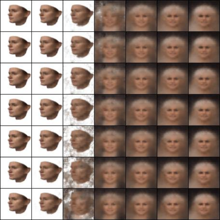
With the aim at reinforcing the robustness of UG-VAE in domain alignment, we include in Figure 13 the results of evaluating GMVAE with two clusters () in a similar setup that in section 4.2. A map with the reduced latent space (using t-SNE) of GMVAE is included in Figure 12, where each point represents an encoded image. Figure 13 shows the interpolation between images of two different domains. As GMVAE does not have global variables, the interpolation applies only for the latent encodings in z. Note that the interpolation is merely a gradual overlap between the two images. Namely, the model is not able to correlate the features of both images, regardless of their domain. On the other hand, with UG-VAE, by keeping fixed the global variable and interpolating in the local one, we maintain the domain but we translate the features of one image into the other. This analysis corroborates that the model finds this type of correlations in a clearly separated way.

A.3 Extended results for Section 4.3: Representation of structured non-trivial data batches
In this extension, we show another evaluation of the capacity of UG-VAE in capturing global structures. In this ocassion, after training the model with randomly picked digits from MNIST, we compute the posterior of structured batches containing only even numbers, only odd numbers, numbers from Fibonacci series, and prime numbers. This grouped batches do not share strong generative factors among them that influence the pixel distributions (as with CelebA groups in experiment 3.3). Namely, the only global information in this example is their frequency of appearance in each batch type. In Figure 14 we show the 2D t-SNE projection of the posterior global latent variable distributions. We observe that UG-VAE is able to discriminate among them in the global space.

Appendix B Networks architecture
In this section we detail the architectures and parameters used for training the models exposed in the main paper. An extended overview is included in Table .