Product Graph Learning from Multi-domain Data with Sparsity and Rank ConstraintsThanks: S.K. Kadambari and S.P. Chepuri are with the Department of Electrical Communication Engineering, Indian Institute of Science, Bangalore, India. E-mail: {kadambarik; spchepuri}@iisc.ac.inThanks: This work is supported in part by the Pratiskha Trust Young Investigator Award and the SERB grant SRG/2019/000619. The precursor version has been published as [1].

The problem of inferring graph topologies from data is ill-posed. Therefore, a graph that best explains the data is often learned by matching the properties of the data to the desired graph and exploiting any prior knowledge available about the desired graph. For an extensive overview on graph learning (also referred to as topology inference) techniques, see [12] and [13] (and references therein).

Although a sample correlation or similarity graph (e.g., $k$-nearest neighbor graph or Gaussian similarity kernel) [7] computed from data are simple graph learning methods, they are sensitive to noise or missing samples as they do not take into account any available prior information about the desired graph or data model. There are two commonly used data models when learning undirected graphs from data. The first model is a probabilistic graphical model of random graph data. In this data model, the assumption is that the graph structure is related to the inverse data covariance matrix (or the so-called precision matrix) that encodes conditional independence relationship of random variables indexed by the nodes. Graph learning, in this case, reduces to finding a maximum likelihood estimator of the inverse covariance matrix by modeling it as a regularized graph Laplacian matrix [17]. The second model is a smoothness model based on the quadratic total variation of data over the graph or sparsity in a basis related to the graph. Graph learning under the smoothness model amounts to finding a graph Laplacian matrix that promotes a smooth variation of the data over the desired graph [8].

Typically we are interested in learning graphs that capture well the local interactions that many real-world datasets exhibit. Thus to obtain useful and meaningful graphs, we seek graph Laplacian matrices that are sparse with very few nonzero entries [8, 9]. Next to a sparsity prior, it is also useful for graph-based clustering applications to infer graphs by incorporating spectral priors to obtain, for instance, multi-component or bipartite graphs [7, 18, 15].

In this work, we restrict our focus to a smoothness data model for structured graph learning, in which we consider a specific structure for the graph in the vertex domain, namely, the product structure. Specifically, we focus on Cartesian product graphs with two smaller graph factors. Cartesian product graphs are useful to explain complex relationships in multi-domain graph data. For instance, consider a rating matrix in a recommender system such as Netflix or Amazon. It has a user dimension as well as an item or a movie dimension. The graph underlying such multi-domain data can often be factorized into a user graph and an item or a movie graph. Furthermore, the graph Laplacian matrix of a Cartesian product graph has a Kronecker sum structure with many interesting spectral properties that allow us to infer such graphs efficiently, or to perform graph filtering [2] and sampling [5] over product graphs efficiently.

Assuming a probabilistic graphical data model, [19] presented Bigraphical Lasso (BiGLasso) —an algorithm for estimating precision matrices with a Kronecker sum structure. Although BiGLasso is not intended to estimate the Laplacian matrices of the graph factors that we are interested in this work, we can always project the inverse covariance matrices obtained from BiGLasso onto the space of valid Laplacian matrices to get a naive estimate of the Laplacian matrices of the graph factors (see Section VI for more details).

In a closely related work in [20], the authors also consider the problem of inferring product graphs as in the precursor [1] of the paper, but without imposing sparsity or spectral constraints on the sought graph. The paper extends the precursor [1] in various aspects, which we summarize in the next section as the main results.

This paper focuses on inferring undirected sparse Cartesian product graphs having two smaller undirected graph factors. We learn these graph factors by estimating the associated graph Laplacian matrices for the following cases.

• •

  We assume a smoothness data model and propose a convex optimization problem for estimating the Laplacian matrices of the graph factors. We present a generative model based on a Kronecker-structured factor analysis model. This model allows us to draw a connection between the smooth variation of data over the product graph and its graph factors. We develop an iterative algorithm to solve the proposed problem optimally by exploiting the symmetric structure of the Laplacian matrices. For a Cartesian product graph with $N$ nodes having graph factors with $P$ and $Q$ nodes such that $N=PQ$, the proposed algorithm incurs a significantly lower computational complexity of about order $P^{2}+Q^{2}$ flops, whereas existing algorithms that do not leverage the Cartesian product structure costs about order $N^{2}$ flops.

• •

  For spectral clustering and subspace representation involving Cartesian product graphs, we extend the framework to learn Cartesian product graphs with multiple connected components by constraining the rank of the Laplacian matrices. For the resulting nonconvex optimization, we develop a solver based on cyclic minimization. Each subproblem of this cyclic minimization algorithm is solved optimally. As we see later, a $K$-component Cartesian product graph with $N$ nodes has $K_{P}$- and $K_{Q}$-component graph factors with $P$ and $Q$ nodes, respectively, such that $K=K_{P}K_{Q}$ and $N=PQ$. To estimate a $K$-component Cartesian product graph to perform graph clustering, the proposed algorithm incurs a computational complexity of about order $K_{P}P^{2}+K_{Q}Q^{2}$ flops that otherwise would cost about order $KN^{2}$ flops.

• •

  Working with smaller graph factors is computationally more attractive. However, not all graphs admit an exact Cartesian product factorization. In such cases, it is useful to approximate the graph of interest by a Cartesian product of two smaller graphs. To this end, we develop algorithms to find a nearest Kronecker sum factorization of a Laplacian matrix to compute the Laplacian matrices of the graph factors. We develop algorithms to obtain sparse and multi-connected graph factors as before.

We demonstrate the usefulness of the developed algorithms through numerical experiments on synthetic and real datasets. The real datasets considered are related to air quality monitoring in India and object classification from multi-view images.

Throughout this paper, we will use upper and lower case boldface letters to denote matrices and column vectors. We will use calligraphic letters to denote sets. $|\cdot|$ denotes the cardinality of the set. $\mathbb{R}_{+}^{N}$ denotes the set of vectors of length $N$ with nonnegative real entries. $\mathbb{S}_{+}^{N}$ ($\mathbb{S}_{++}^{N}$) denotes the set of symmetric positive semidefinite (positive definite) matrix of size $N\times N$. $[{\mathbf{X}}]_{ij}$ and $x_{i}$ denote the $(i,j)$th element and $i$th element of the matrix ${\mathbf{X}}$ and vector ${\mathbf{x}}$, respectively. ${\mathbf{I}}_{P}$ denotes the identity matrix of size $P$. $\rm diag[\cdot]$ ($\rm bdiag[\cdot]$) is a (block) diagonal matrix with its argument along the main diagonal. ${\rm tr}(\cdot)$ is the trace of the matrix. ${\rm vec}(\cdot)$ is the matrix vectorization operation. ${\rm vech}(\cdot)$ is the half-vectorization of a symmetric matrix obtained by vectorizing only the lower triangular part of the matrix. $\lambda_{i}(\cdot)$ denotes the $i$th smallest eigenvalue of its symmetric matrix argument. The symbols $\oplus$ and $\otimes$ represents the Kronecker sum and the Kronecker product, respectively. The symbol $\diamond$ denotes the Cartesian product between two graphs. ${\mathbf{x}}\succeq{\mathbf{y}}$ denotes elementwise inequality between vectors ${\mathbf{x}}$ and ${\mathbf{y}}$. The operator $\texttt{mat}({\mathbf{x}},M,N)$ returns the $M\times N$ matrix obtained by arranging entries of the vector ${\mathbf{x}}$ having $MN$ entries in column-major order.

We frequently use the following identities. For matrices ${\mathbf{A}}$, ${\mathbf{B}}$, ${\mathbf{C}}$ and ${\mathbf{X}}$ of appropriate dimensions, the equation ${\mathbf{A}}{\mathbf{X}}+{\mathbf{X}}{\mathbf{B}}={\mathbf{C}}$ is equivalent to $({\mathbf{A}}\oplus{\mathbf{B}}^{T}){\rm vec}({\mathbf{X}})={\rm vec}({\mathbf{C}})$ and ${\rm vec}({\mathbf{A}}{\mathbf{B}}{\mathbf{C}})=({\mathbf{C}}^{T}\otimes{\mathbf{A}}){\rm vec}({\mathbf{B}})$. The Kronecker sum of two matrices ${\mathbf{A}}\in{\mathbb{R}}^{M\times M}$ and ${\mathbf{B}}\in{\mathbb{R}}^{N\times N}$ can be expressed as ${\mathbf{A}}\oplus{\mathbf{B}}={\mathbf{I}}_{N}\otimes{\mathbf{A}}+{\mathbf{B}}\otimes{\mathbf{I}}_{M}$. The trace of the product of two matrices can be expressed as ${\rm tr}({\mathbf{A}}^{T}{\mathbf{X}})={\rm vec}({\mathbf{A}})^{T}{\rm vec}({\mathbf{X}})$. Thus we have ${\rm tr}({{\mathbf{A}}}^{T}{{\mathbf{A}}})=\|{{\mathbf{A}}}\|_{F}^{2}={\rm vec}({{\mathbf{A}}})^{T}{\rm vec}({{\mathbf{A}}})$. For an $N\times N$ symmetric and positive semidefinite matrix ${\mathbf{A}}$, we have [21, Proposition 1.3.4]

We compactly denote the optimal solution ${\mathbf{V}}$ that contains as columns the $K$ eigenvectors corresponding to the $K$ smallest eigenvalues of ${\mathbf{A}}$ as ${\mathbf{V}}=\texttt{eigs}({\mathbf{A}},K)$.

The remainder of the paper is organized as follows. In Sections II and III, we discuss product graphs, subspace representation of product graphs, product graph signals, and a generative model for smooth product graph signals. In Section IV, we develop algorithms for estimating graph factors from data. In Section V, we present algorithms for finding a nearest Kronecker sum factorization for approximating a graph by a Cartesian product graph. We discuss the results from numerical experiments performed on synthetic and real datasets in Section VI. The paper is concluded in Section VII.

Consider a weighted undirected graph ${\mathcal{G}}_{N}=({\mathcal{V}}_{N},{\mathcal{E}}_{N})$ with $N$ nodes (or vertices). The sets ${\mathcal{V}}_{N}$ and ${\mathcal{E}}_{N}$ denote the vertex set and edge set, respectively. The structural connectivity of the graph ${\mathcal{G}}_{N}$ is represented by the symmetric adjacency matrix ${\mathbf{W}}_{N}\in{\mathbb{R}}^{N\times N}$. The $(i,j){\rm th}$ entry of ${\mathbf{W}}_{N}$ is positive if there is an edge between node $i$ and node $j$. We also assume that the graph ${\mathcal{G}}_{N}$ has no self-loops. Thus the diagonal entries of ${\mathbf{W}}_{N}$ are all zero. The diagonal node degree matrix of the graph ${\mathcal{G}}_{N}$ is given by ${\rm diag}\left[{\mathbf{W}}_{N}{\bf 1}_{N}\right]\in{\mathbb{R}}^{N\times N}$. The graph Laplacian matrix ${\mathbf{L}}_{N}\in\mathbb{S}_{+}^{N}$ associated with the graph ${\mathcal{G}}_{N}$ is defined as ${\mathbf{L}}_{N}={\rm diag}\left[{\mathbf{W}}_{N}{\bf 1}_{N}\right]-{\mathbf{W}}_{N}$.

By construction the graph Laplacian matrix of an undirected graph is real, symmetric, and positive semidefinite. Thus ${\bf L}_{N}$ admits the following decomposition

where ${\mathbf{U}}_{N}\in{\mathbb{R}}^{N\times N}$ is an orthonormal matrix that contains the eigenvectors $\{{\mathbf{u}}_{1},\cdots,{\mathbf{u}}_{N}\}$ as its columns and $\boldsymbol{\Lambda}_{N}$ is a diagonal matrix that contains along its diagonal the eigenvalues $\{\lambda_{1}({\mathbf{L}}_{N}),\cdots,\lambda_{N}({\mathbf{L}}_{N})\}$. We assume that the eigenvalues are ordered as $0=\lambda_{1}({\mathbf{L}}_{N})\leq\lambda_{2}({\mathbf{L}}_{N})\leq\cdots\leq\lambda_{N}({\mathbf{L}}_{N})$. Furthermore, the all-one vector lies in null space of ${\mathbf{L}}_{N}$, i.e., ${\mathbf{u}}_{1}={\bf 1}_{N}$, without loss of generality. Thus we may denote the space of all the valid combinatorial Laplacian matrices of size $N$ by the set

In this above set, the inequality $[{\mathbf{L}}]_{ii}\geq 0$ is implicit. Furthermore, the symmetric Laplacian matrix ${\mathbf{L}}_{N}$ can be compactly represented with the $M_{N}=N(N+1)/2$ nonduplicated elements ${\boldsymbol{l}}_{N}\in\mathbb{R}_{+}^{M_{N}}$ as

where ${\boldsymbol{l}}_{N}\succeq{\bf 0}$ and the duplication matrix ${\mathbf{D}}_{N}$ of size $N^{2}\times~M_{N}$ is explicitly expressed as

Here, ${\boldsymbol{\delta}}_{ij}\in\mathbb{R}^{M_{N}}$ is the canonical vector with 1 at position $(j-1)N+i-0.5j(j-1)$, and zero elsewhere. The matrix ${\boldsymbol{\Theta}}_{ij}\in\mathbb{R}^{N\times N}$ is the canonical symmetric matrix with the value $-1$ in the position $(i,j)$, $1$ at the position $(i,i)$, and zero elsewhere, for all $i,j$.

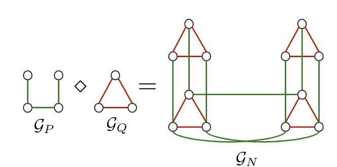
Consider two graphs ${\mathcal{G}}_{P}=({\mathcal{V}}_{P},{\mathcal{E}}_{P})$ and ${\mathcal{G}}_{Q}=({\mathcal{V}}_{Q},{\mathcal{E}}_{Q})$ having $P$ and $Q$ nodes, respectively. Let ${\mathbf{L}}_{P}\in\mathbb{S}_{+}^{P}$ and ${\mathbf{L}}_{Q}\in\mathbb{S}_{+}^{Q}$ be the graph Laplacian matrices of ${\mathcal{G}}_{P}$ and ${\mathcal{G}}_{Q}$, respectively. We assume that the graph ${\mathcal{G}}_{N}$ can be factorized into two factors such that the Cartesian product of the graphs ${\mathcal{G}}_{P}$ and ${\mathcal{G}}_{Q}$ is ${\mathcal{G}}_{N}$, that is,

In other words, the graphs ${\mathcal{G}}_{P}$ and ${\mathcal{G}}_{Q}$ form the graph factors of the Cartesian product graph ${\mathcal{G}}_{N}$. The number of nodes in the Cartesian product graph ${\mathcal{G}}_{N}$ is $N=PQ$. An illustration of a Cartesian product graph with $N=12$ nodes and graph factors having $P=3$ and $Q=4$ nodes is shown in Fig. 1(a).

The graph Laplacian matrix ${\mathbf{L}}_{N}$ of ${\mathcal{G}}_{N}$ can be expressed in terms of the Laplacian matrices of its graph factors ${\mathcal{G}}_{P}$ and ${\mathcal{G}}_{Q}$ as [2]

Similar to (4), we can compactly represent ${\mathbf{L}}_{P}$ and ${\mathbf{L}}_{Q}$ as

where ${\boldsymbol{l}}_{P}\in\mathbb{R}^{M_{P}}_{+}$ with $M_{P}=P(P+1)/2$ and ${\boldsymbol{l}}_{Q}\in\mathbb{R}^{M_{Q}}_{+}$ with $M_{Q}=Q(Q+1)/2$. Here, ${\mathbf{D}}_{P}\in\mathbb{R}^{P^{2}\times M_{P}}$ and ${\mathbf{D}}_{Q}\in\mathbb{R}^{Q^{2}\times M_{Q}}$ are the duplication matrices defined in (5). We later on use the fact that the matrices ${\mathbf{D}}_{P}^{T}{\mathbf{D}}_{P}\in\mathbb{S}_{++}^{M_{P}}$ and ${\mathbf{D}}_{Q}^{T}{\mathbf{D}}_{Q}\in\mathbb{S}_{++}^{M_{Q}}$ are diagonal.

Let us denote the eigenvalue decomposition of the Laplacian matrices ${\mathbf{L}}_{P}$ and ${\mathbf{L}}_{Q}$ as ${\mathbf{L}}_{P}={\mathbf{U}}_{P}\boldsymbol{\Lambda}_{P}{\mathbf{U}}_{P}^{T}$ and ${\mathbf{L}}_{Q}={\mathbf{U}}_{Q}\boldsymbol{\Lambda}_{Q}{\mathbf{U}}_{Q}^{T}$, respectively. Here, ${\mathbf{U}}_{P}\in{\mathbb{R}}^{P\times P}$ and ${\mathbf{U}}_{Q}\in{\mathbb{R}}^{Q\times Q}$ are the eigenvector matrices, and $\boldsymbol{\Lambda}_{P}\in{\mathbb{R}}^{P\times P}$ and $\boldsymbol{\Lambda}_{Q}\in{\mathbb{R}}^{Q\times Q}$ are the matrices of eigenvalues. Then the eigenvalue decomposition of ${\mathbf{L}}_{N}$ can be expressed as [22]

This means that, the eigenvector matrix has a Kronecker product structure ${\mathbf{U}}_{N}={\bf U}_{Q}\otimes{\bf U}_{P}$ and the eigenvalue matrix has a Kronecker sum structure $\boldsymbol{\Lambda}_{N}={\boldsymbol{\Lambda}}_{P}\oplus{\boldsymbol{\Lambda}}_{Q}$. This Kronecker structure can be exploited to efficiently perform clustering on product graphs as discussed next.

The algebraic multiplicity of the zero eigenvalue of a graph Laplacian matrix determines the number of connected components of the graph [23]. This means that the rank of the graph Laplacian matrix of a $K$-connected graph with $N$ nodes is $N-K$. The matrix containing the $K$ eigenvectors associated with the $K$ smallest eigenvalues of the graph Laplacian yields a low-dimensional node representation (i.e., a $K$-dimensional node embedding), which preserves the information about the connectivity of the nodes in the graph. In particular, the $n$th row of this matrix forms the coordinates of the $n$th node in the low-dimensional subspace and is used for clustering the nodes of the graph [24].

A direct consequence of the Kronecker sum structure of the eigenvalue matrix in (8) is that a $K$-component product graph can be equivalently represented as the Cartesian product of two smaller graph factors having $K_{P}$ and $K_{Q}$ components with $K=K_{P}K_{Q}$. Suppose the graph ${\mathcal{G}}_{N}={\mathcal{G}}_{P}\diamond{\mathcal{G}}_{Q}$ has $K$ connected components. Then we have ${\rm rank}({\mathbf{L}}_{N})=N-K$, ${\rm rank}({\mathbf{L}}_{P})=P-K_{P}=R_{P}$, ${\rm rank}({\mathbf{L}}_{Q})=Q-K_{Q}=R_{Q}$. Further, from (8), the $K_{P}$-dimensional and $K_{Q}$-dimensional node embeddings can be used to efficiently compute the $K$-dimensional representation for ${\mathcal{G}}_{N}$. This is particularly useful in reducing the computational costs incurred while clustering large graphs.

A smoothness metric based on the quadratic total variation with respect to the underlying graph Laplacian matrix is often used to quantify how well the signal ${\mathbf{x}}_{i}$ is related to the supporting graph. Specifically, we define the metric

which penalizes signals ${\mathbf{x}}_{i}$ for which neighboring nodes have very different values. Clearly, for constant signals, this quadratic term is zero. For Cartesian product graphs [cf. (6)], this smoothness promoting quadratic term can be explicitly expressed in terms of its graph factors as

This means that the quadratic norm induced by the Cartesian product graph is separable and can be simplified as the sum of the quadratic total variation of the signals collected in the rows and columns of ${\mathbf{X}}_{i}$ with respect to its graph factors ${\mathcal{G}}_{P}$ and ${\mathcal{G}}_{Q}$. For $T$ snapshots of the data, this quadratic norm generalizes as

where we have defined the sample data covariance matrices ${\mathbf{S}}_{P}=\sum\limits_{i=1}^{T}{\mathbf{X}}_{i}{\mathbf{X}}_{i}^{T}\in\mathbb{R}^{P\times P}$ and ${\mathbf{S}}_{Q}=\sum\limits_{i=1}^{T}{\mathbf{X}}_{i}^{T}{\mathbf{X}}_{i}\in\mathbb{R}^{Q\times Q}$.

Next, we describe a generative model for the multi-domain data that vary smoothly across the edges of a product graph in terms of its graph factors. The presented modeling is an extension of the factor analysis model for single domain datasets [8] to multi-domain data.

Since the eigenvector matrix ${\mathbf{U}}_{N}$ has a Kronecker product structure, we can synthesize ${\mathbf{x}}_{i}$ as

where $\tilde{{\mathbf{x}}}_{i}={\rm vec}(\tilde{{\mathbf{X}}}_{i})$. Let us consider a noisy version of ${\bf X}_{i}$ given by

where ${\mathbf{Y}}_{i}\in{\mathbb{R}}^{P\times Q}$ is the $i$th snapshot of the multi-domain noisy graph data, ${\bf E}_{i}\in\mathbb{R}^{P\times Q}$ is the observation noise, and $\tilde{\bf X}_{i}\in{\mathbb{R}}^{P\times Q}$ is the latent factor matrix with loading matrices ${\mathbf{U}}_{P}$ and ${\mathbf{U}}_{Q}$, which jointly influence the observations ${\mathbf{Y}}_{i}$.

On vectorizing (12), we get

where ${\mathbf{y}}_{i}\in{\mathbb{R}}^{PQ}$ with ${\mathbf{y}}_{i}={\rm vec}({\mathbf{Y}}_{i})$. We assume that ${\bf e}_{i}={\rm vec}({\bf E}_{i})$ is distributed as ${\bf e}_{i}\sim{\mathcal{N}}({\bf 0},\sigma^{2}{\mathbf{I}}_{N})$. We refer to this model as the Kronecker-structured factor analysis model.

Next, we define a Gaussian prior distribution $p(\tilde{\bf x}_{i})$ over the latent factors along with a Gaussian conditional distribution $p({\bf y}_{i}|\tilde{\bf x}_{i})$ for the observed variable ${\bf y}_{i}$ conditioned on the value of the latent variable $\tilde{\bf x}_{i}$. More specifically, the prior distribution over $\tilde{\bf x}_{i}$ is given by

where $[\boldsymbol{\Lambda}_{P}\oplus\boldsymbol{\Lambda}_{Q}]^{\dagger}\in\mathbb{R}^{N\times N}$ is a diagonal matrix and the conditional distribution of ${\bf y}_{i}$ conditioned on $\tilde{\bf x}_{i}$ is given by

Then the maximum a posteriori (MAP) estimate of $\tilde{{\mathbf{x}}}_{i}$ is

where the constant $\alpha>0$ is related to the noise variance $\sigma^{2}$. Using (11) in (15) and from (9), the MAP estimate of ${{\mathbf{X}}}_{i}$ is obtained by solving

This means that the data that follows the Kronecker-structured factor analysis model (12) with a Gaussian prior on the latent factors as in (14) yield graph data that are simulatenously smooth on the graph factors of the Cartesian product graph. More generally, we can jointly denoise $T$ snapshots of the noisy data ${\mathbf{Y}}_{i}$, for $i=1,\ldots,T$, using the graph regularizer in (10), as

In what follows, based on (16), we formulate product graph learning as the problem of estimating the Laplacian matrices of the graph factors underlying the available data.

We jointly estimate ${\mathbf{L}}_{P}$ and ${\mathbf{L}}_{Q}$ by restricting our search to the set of Laplacian matrices defined in (3). That is, we propose to solve the following product graph learning (PGL) problem:

where the trace equality constraints avoid the trivial solution. It can be shown that ${\rm tr}({\mathbf{L}}_{i})=2\|{\rm vec}({\mathbf{W}}_{i})\|_{1}$, which is a commonly used convex approximation of the sparsity-inducing $\ell_{0}$-norm penalty. Since constraining $\|{\rm vec}({\mathbf{W}}_{i})\|_{1}$ for $i\in\{P,Q\}$, in this case, only changes the scale of the solution, we propose to choose the penalty term

with parameters $\beta_{1}>0$ and $\beta_{2}>0$ in the objective to control the sparsity of ${\mathcal{G}}_{P}$ and ${\mathcal{G}}_{Q}$, respectively, by controlling the distribution of the edge weights. See [10] for other regularizers that may be used to obtain sparse graphs. Given ${\mathbf{S}}_{P}$ and ${\mathbf{S}}_{Q}$, the optimization problem ( ⁢ P 1 ) is convex in ${\mathbf{L}}_{P}$ and ${\mathbf{L}}_{Q}$.

Now, we present a very efficient solver for ( ⁢ P 1 ), by exploiting the symmetric structure of the Laplacian matrices and by compactly representing it using (7). Let us define ${\boldsymbol{l}}\in\mathbb{R}_{+}^{M}$ with $M=M_{P}+M_{Q}$ as ${\boldsymbol{l}}=[{\boldsymbol{l}}_{P}^{T},{\boldsymbol{l}}_{Q}^{T}]^{T}$. Using the identities

and

for $i\in\{P,Q\}$, the optimization problem ( ⁢ P 1 ) can equivalently be written as

with known parameters ${\rm diag}({\mathbf{p}}_{\rm d})\in\mathbb{S}_{++}^{M}$, ${\mathbf{q}}_{\rm d}\in\mathbb{R}^{M}$, ${\mathbf{C}}\in~\mathbb{R}^{L\times M}$, and ${\mathbf{d}}\in\mathbb{R}^{L}$, where $L=P+Q+2$. Here,

and

The subscript “${\rm d}$” represents parameters related to the data. The parameters related to the equality constraints are [see Appendix -A]

with

for $i\in\{P,Q\}$.

The optimization problem (17) is a special case of a quadratic program in which the matrix associated with the quadratic term in the objective function is diagonal. This optimization problem can be solved efficiently and optimally using Algorithm 1, which is developed in Appendix -B. The optimal solution to ( ⁢ P 1 ) is given by the iterative procedure

Although we concatenate ${\boldsymbol{l}}_{P}$ and ${\boldsymbol{l}}_{Q}$, and present a solver for ${\boldsymbol{l}}$ as described above, it is computationally less expensive to solve for ${\boldsymbol{l}}_{P}$ and ${\boldsymbol{l}}_{Q}$ separately as it is easy to see that the problem is separable in these variables. Specifically, the solution to ( ⁢ P 1 ) is given by ${\boldsymbol{l}}_{i}^{\star}=\texttt{PGL}({\mathbf{p}}_{{\rm d},i},{\mathbf{q}}_{{\rm d},i},{\mathbf{C}}_{i},{\mathbf{d}}_{i},\texttt{Tol},\rho)$ for $i\in\{P,Q\}$. By doing so, we incur a per iteration computational cost of the order $P^{2}+Q^{2}$ flops (cf. Appendix -B) and not order $(P+Q)^{2}$ flops.

In the next section, we specialize the problem of learning sparse graph factors discussed in this section to the specific case in which the graphs ${\mathcal{G}}_{P}$ and ${\mathcal{G}}_{Q}$ each have multiple connected components.

As discussed in Section II-C, if the underlying graph has a product structure, then instead of learning a large multi-component graph with $N$ nodes, we may learn smaller multi-component graph factors with $P$ and $Q$ nodes, or learn the low-dimensional embeddings of the nodes in ${\mathcal{G}}_{N}$, by computing the low-dimensional representations for ${\mathcal{G}}_{P}$ and ${\mathcal{G}}_{Q}$.

Suppose that the graphs ${\mathcal{G}}_{P}$ and ${\mathcal{G}}_{Q}$ have $K_{P}$ and $K_{Q}$ connected components, respectively. Although tuning $\beta_{1}$ and $\beta_{2}$ in ( ⁢ P 1 ) allows us to control the sparsity of the edge weights, we cannot, however, obtain graphs with a desired number of connected components. Therefore, we specialize ( ⁢ P 1 ) to learn graphs factors with multiple connected components by solving the following rank-constrained product graph learning (RPGL) problem

where $R_{P}=P-K_{P}$ and $R_{Q}=Q-K_{Q}$. Recall that the rank constraints ensure that the algebraic multiplicity of the zero eigenvalue of ${\mathbf{L}}_{P}$ and ${\mathbf{L}}_{Q}$ are, respectively, $K_{P}$ and $K_{Q}$. In [18], a similar rank constraint was used to refine an affinity graph (with no product structure) for spectral clustering. In contrast to Problem ( ⁢ P 1 ), the optimization problem ( ⁢ P 2 ) is a nonconvex optimization problem. Although the trace equality constraints are not required anymore to avoid a trivial solution, we retain them here as it will be required when we solve Problem ( ⁢ P 2 ) using a cyclic minimization technique as discussed next.

Let us denote the cost function in ( ⁢ P 2 ) as

As ${\mathbf{L}}_{P}\succeq{\bf 0}$ and ${\mathbf{L}}_{Q}\succeq{\bf 0}$, we can rewrite ( ⁢ P 2 ) as

where the tuning parameters $\gamma_{1}>0$ and $\gamma_{2}>0$ force the second and third terms of the objective to zero at optimality ensuring the rank of the optimal ${\mathbf{L}}_{P}$ and ${\mathbf{L}}_{Q}$ to be $R_{P}$ and $R_{Q}$, respectively. From (1), Problem (21) will then be

with variables ${\mathbf{L}}_{P}\in\mathbb{S}_{+}^{P}$, ${\mathbf{L}}_{Q}\in\mathbb{S}_{+}^{Q}$, ${\mathbf{V}}_{P}\in\mathbb{R}^{P\times K_{P}}$, and ${\mathbf{V}}_{Q}\in\mathbb{R}^{Q\times K_{Q}}$. The optimization problem (22) is not a convex optimization problem. Therefore, we propose to solve it by alternatingly minimizing it with respect to $\{{\mathbf{L}}_{P},{\mathbf{L}}_{Q}\}$ and $\{{\mathbf{V}}_{P},{\mathbf{V}}_{Q}\}$, while keeping the other variable fixed. For each subproblem, we achieve the global optimum.

To compute the Laplacian matrices ${\mathbf{L}}_{P}$ and ${\mathbf{L}}_{Q}$ from ${\mathbf{L}}_{N}$, we propose the following Kronecker sum factorization (KronFact) problem

where the trace constraints are used to fix the scales of ${\mathbf{L}}_{P}$ and ${\mathbf{L}}_{Q}$. The constraint sets ${\mathcal{L}}_{P}$ and ${\mathcal{L}}_{Q}$ are the sets of all the valid combinatorial Laplacian matrices of size $P\times P$ and $Q\times Q$, respectively [cf. (3) for the definition].

The optimization problem ( ⁢ P 3 ) can be equivalently expressed as the following convex optimization problem [see Appendix -C]

with known parameters ${\rm diag}({\mathbf{p}}_{\rm f})\in\mathbb{S}_{++}^{M}$, ${\mathbf{q}}_{\rm f}\in\mathbb{R}^{M}$, ${\mathbf{C}}\in~\mathbb{R}^{L\times M}$, and ${\mathbf{d}}\in\mathbb{R}^{L}$, where recall that $L=P+Q+2$. The subscript “${\rm f}$” represents factorization. The parameters in the objective function are defined as

and

where ${\tilde{\mathbf{L}}}_{N}\in\mathbb{R}^{Q^{2}\times P^{2}}$ is the tilde transform of ${\mathbf{L}}_{N}$ defined in (37) and (38). The parameters related to the equality constraints are defined in (20) [see Appendix -A].

Although the need for the trace equality constraints is not evident in ( ⁢ P 3 ), it is easy to realize that without the trace equality constraints, (25) will result in a trivial solution. Further, Problems (17) and (25) have similar form. The role of $\beta_{1}$ and $\beta_{2}$ in (17) to control the sparsity and distribution of edge weights is now played by $P$ and $Q$, respectively.

As seen before, the optimization problem (25) can be solved efficiently and optimally using Algorithm 1. Specifically, the optimal solution to ( ⁢ P 3 ) is given as ${\boldsymbol{l}}^{\star}=\texttt{PGL}({\mathbf{p}}_{\rm f},{\mathbf{q}}_{\rm f},{\mathbf{C}},{\mathbf{d}},\texttt{Tol},\rho)$. It is computationally less expensive to solve for ${\boldsymbol{l}}_{P}$ and ${\boldsymbol{l}}_{Q}$ separately as earlier.

To compute the graph factors ${\mathcal{G}}_{P}$ and ${\mathcal{G}}_{Q}$ with $K_{P}$ and $K_{Q}$ components, respectively, we propose to factorize the available ${\mathbf{L}}_{N}$ to estimate ${\mathbf{L}}_{P}$ and ${\mathbf{L}}_{Q}$ using ( ⁢ P 3 ) with rank constraints as in ( ⁢ P 2 ). Specifically, we propose to solve the following rank-constrained Kronecker sum factorization (R-KronFact) problem

References

- [1] S. K. Kadambari and S. P. Chepuri, “Learning product graphs from multidomain signals,” in Proc. of the IEEE Int. Conf. on Acoustics, Speech and Signal Process. (ICASSP), Barcelona, Spain, May 2020.
- [2] A. Sandryhaila and J. M. Moura, “Big data analysis with signal processing on graphs: Representation and processing of massive data sets with irregular structure,” IEEE Signal Process. Mag., vol. 31, no. 5, pp. 80–90, Sep. 2014.
- [3] D. I. Shuman, S. K. Narang, P. Frossard, A. Ortega, and P. Vandergheynst, “The emerging field of signal processing on graphs: Extending high-dimensional data analysis to networks and other irregular domains,” IEEE Signal Process. Mag., vol. 30, no. 3, pp. 83–98, May 2013.
- [4] S. Chen, R. Varma, A. Sandryhaila, and J. Kovacevic, “Discrete signal processing on graphs: Sampling theory,” IEEE Trans. Signal Process., vol. 63, no. 24, pp. 6510–6523, Dec. 2015.
- [5] G. Ortiz-Jiménez, M. Coutino, S. P. Chepuri, and G. Leus, “Sparse sampling for inverse problems with tensors,” IEEE Trans. Signal Process., vol. 67, no. 12, pp. 3272–3286, June 2019.
- [6] S. P. Chepuri and G. Leus, “Graph sampling for covariance estimation,” IEEE Trans. Signal Inf. Process. Netw., vol. 3, no. 3, pp. 451–466, Sep. 2017.
- [7] U. Von Luxburg, “A tutorial on spectral clustering,” Statistics and computing, vol. 17, no. 4, pp. 395–416, 2007.
- [8] X. Dong, D. Thanou, P. Frossard, and P. Vandergheynst, “Learning Laplacian matrix in smooth graph signal representations,” IEEE Trans. Signal Process., vol. 64, no. 23, pp. 6160–6173, Dec. 2016.
- [9] S. P. Chepuri, S. Liu, G. Leus, and A. O. Hero III, “Learning sparse graphs under smoothness prior,” in Proc. of the IEEE Int. Conf. on Acoustics, Speech and Signal Process. (ICASSP), New Orleans, USA, Mar. 2017.
- [10] V. Kalofolias, “How to learn a graph from smooth signals,” in Proc. of Artificial Intelligence and Statistics (AISTATS), Cadiz, Spain, May 2016, pp. 920–929.
- [11] H. E. Egilmez, E. Pavez, and A. Ortega, “Graph learning from data under Laplacian and structural constraints,” IEEE J. Sel. Topics Signal Process., vol. 11, no. 6, pp. 825–841, Sep. 2017.
- [12] X. Dong, D. Thanou, M. Rabbat, and P. Frossard, “Learning graphs from data: A signal representation perspective,” IEEE Signal Process. Mag., vol. 36, no. 3, pp. 44–63, May 2019.
- [13] G. Mateos, S. Segarra, A. G. Marques, and A. Ribeiro, “Connecting the dots: Identifying network structure via graph signal processing,” IEEE Signal Process. Mag., vol. 36, no. 3, pp. 16–43, May 2019.
- [14] S. P. Chepuri, M. Coutino, A. G. Marques, and G. Leus, “Distributed analytical graph identification,” in Proc. of the IEEE Int. Conf. on Acoustics, Speech and Signal Process. (ICASSP), Calgary, Canada, Apr. 2018.
- [15] S. Kumar, J. Ying, J. V. de Miranda Cardoso, and D. Palomar, “Structured graph learning via Laplacian spectral constraints,” in Proc. of Advs. in Neural Inf. Proc. Sys. (NeurIPS), Vancouver, Canada, Dec. 2019.
- [16] G. B. Giannakis, Y. Shen, and G. V. Karanikolas, “Topology identification and learning over graphs: Accounting for nonlinearities and dynamics,” Proc. IEEE, vol. 106, no. 5, pp. 787–807, May 2018.
- [17] B. Lake and J. Tenenbaum, “Discovering structure by learning sparse graphs,” Proc. 32nd Annu. Meeting Cognitive Science Society (CogSci), pp. 778 – 784, Aug. 2010.
- [18] F. Nie, X. Wang, M. I. Jordan, and H. Huang, “The constrained laplacian rank algorithm for graph-based clustering.” in Proc. of the Thirtieth AAAI Conf. on Artificial Intelligence, Arizona USA, Feb. 2016.
- [19] A. Kalaitzis, J. Lafferty, N. D. Lawrence, and S. Zhou, “The bigraphical lasso,” in Proc. of the 30th Int. Conf. on Machine Learning, vol. 28, no. 3, Atlanta, Georgia, USA, June 2013.
- [20] M. A. Lodhi and W. U. Bajwa, “Learning product graphs underlying smooth graph signals,” 2020.
- [21] T. Tao, Topics in random matrix theory. American Mathematical Soc., 2012.
- [22] R. A. Horn, R. A. Horn, and C. R. Johnson, Topics in matrix analysis. Cambridge university press, 1994.
- [23] D. Spielman, “Spectral graph theory,” in U. Naumann and O. Schenk (Ed.), Combinatorial scientific computing. CRC Press, 2012.
- [24] A. Y. Ng, M. I. Jordan, and Y. Weiss, “On spectral clustering: Analysis and an algorithm,” in Proc. of the Adv. in neural inf. proc. sys. (NIPS), Vancouver, Canada, Dec. 2002.
- [25] L. K. Saul and S. T. Roweis, “An introduction to locally linear embedding,” unpublished. Available at: http://www..nyu.edu/˜roweis/lle/publications.html, Jan. 2001.
- [26] “Central control room for air quality management, India,” https://app.cpcbccr.com/.
- [27] S. Nane, S. Nayar, and H. Murase, “Columbia object image library: Coil-20,” Dept. Comp. Sci., Columbia University, New York, Tech. Rep, Feb. 1996.
- [28] T. Hastie, R. Tibshirani, and J. Friedman, The elements of statistical learning. New York: Springer, 2001.
- [29] R. H. Koning, H. Neudecker, and T. Wansbeek, “Block Kronecker products and the vecb operator,” Linear algebra and its applications, vol. 149, pp. 165–184, Aug. 1990.