A Novel Sum-Product Detection Algorithm for Faster-than-Nyquist Signaling: A Deep Learning Approach B. Liu, S. Li, Y. Xie and J. Yuan are with the School of Electrical Engineering and Telecommunications, the University of New South Wales, Sydney, Australia (e-mail: {bryan.liu, shuangyang.li, yixuan.xie, j.yuan}@unsw.edu.au). This paper was presented in part at the 2019 IEEE Information Theory Workshop (ITW) [1].

Without loss of generality, the considered coded FTN system model is shown in Fig. 1. Let $\bm{b}$ denote the binary source data with length $K$. At the transmitter, $\bm{b}$ is convolutionally encoded, resulting in a binary codeword $\bm{c}$ of length $N$. A sequence of $N$ binary phase-shift keying (BPSK) symbols $\mathbf{x}=[x_{1},x_{2},...,x_{N}]^{\text{T}}$ is generated after interleaving the bits in $\bm{c}$ with $x_{i}=(-1)^{c_{i}}$ for $i\in\{1,...,N\}$. The transmitted FTN signals are linear modulation signals of the form $s(t)=\sum_{n}{x_{n}}{h(t-n\tau T)}$, where $\tau$ is the time acceleration factor of the FTN signaling [2] and $h(t)$ is a $T$-orthogonal root raised cosine pulse with a roll-off factor $\alpha$.

Assume that the channel is modelled by additive white Gaussian noises (AWGN) with a zero mean and a variance of $\sigma^{2}$. The received sequence $\bm{y}$ after a matched filtering and FTN rate sampling is given by $\bm{y}=\mathbf{G}\mathbf{x}+\bm{\eta}$, where $\mathbf{G}$ is a Toeplitz generator matrix, as shown below,

The generator matrix consists ISI taps ${g_{i}}=\int_{-\infty}^{\infty}{h\left(t\right){h^{*}}\left({t-i\tau T}\right){\rm{d}}t}$. Specifically, we define $L$ as the number of channel responses with significant energy. The rest ISI taps with insignificant energy are therefore negligible and then set to zeros for simplicity, i.e., ${g_{i}}=0$, for $|i|>L$. Meanwhile, the term $\bm{\eta}$ represents the colored noise samples whose autocorrelation matrix is $\mathbb{E}[\bm{\eta}{\bm{\eta}}^{\rm{H}}]=\sigma^{2}\mathbf{G}$.

Once the sequence $\bm{y}$ is observed, the receiver performs the Turbo equalization, where the extrinsic information from the detector and decoder is exchanged iteratively via the interleaver $\mathbf{\Pi}$ or the deinterleaver ${\mathbf{\Pi}^{-1}}$ until the maximum iteration number is reached. The sequence $\hat{\bm{b}}$ as the estimate of $\bm{b}$ is generated after the Turbo equalization iterations, which is regarded as the output for the receiver.

In this subsection, we briefly review the SPDA proposed in [19]. Given the received sequence $\bm{y}$, the SPDA factorizes the $a\ posterior$ probabilities (APPs) $P(\bm{x}|\bm{y})$ of the transmitted sequence $\bm{x}$ mainly based on three types of FNs:

$\bullet$ $O_{i}(x_{i})$ for $i\in\{1,...N\}$: The $a\ priori$ probability for symbol $x_{i}$ being transmitted.

$\bullet$ $T_{i}(x_{i})$ for $i\in\{1,...N\}$: The symbol likelihood function for symbol $x_{i}$ being transmitted based on the received symbol $y_{i}$.

$\bullet$ $I_{i,j}(x_{i},x_{j})$ for $j\in\{1,...N\}$ and $i\in\{j,...N\}$: The FN that conveys the messages from node $i$ to the interfering node $j$.

The functions of $T_{i}(x_{i})$ and $I_{i,j}(x_{i},x_{j})$ are defined as [19]:

where $x_{i}^{*}$ refers to the conjugate of the symbol $x_{i}$, $\text{Re}\{\cdot\}$ represents the function that returns the real part of a value, and ${\bf{G}}_{i,j}=g_{i-j}$ is the ${(i-j)}$-th ISI tap. It is derived in [19] that $P(\bm{x}|\bm{y})\propto\prod_{i=1}^{N}\bigg[O_{i}(x_{i})T_{i}(x_{i})\prod_{j<i}I_{i,j}(x_{i},x_{j})\bigg]$.

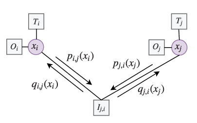
Define $q_{i,j}(x_{i})$ as the message from the FN $I_{i,j}$ to the VN $x_{i}$, $p_{i,j}(x_{i})$ as the message from the VN $x_{i}$ to the FN $I_{i,j}(x_{i},x_{j})$, $o(x_{i})$ as the message from the VN $x_{i}$ to the FN $O_{i}$, and $Q_{i}(x_{i})$ as the product of all messages incoming to the VN $x_{i}$, respectively. Here, $Q_{i}(x_{i})$ indicates the proportional probability of the (approximated) APP $P(x_{i}|\bm{y})$ [19]. An example of part of the FG is given in Fig. 2, where the messages are updated according to [19]:

The messages $\{p_{i,j}\}$ and $\{q_{i,j}\}$ are initialized to the same positive values and the messages are updated iteratively until the maximum number of iterations is reached. Note that the detection complexity of the SPDA is linear to the degree of VNs, i.e., the number of the FNs $I_{i,j}(x_{i})$ linked to each VN $x_{i}$. Therefore, the SPDA provides a trade-off between the detection performance and detection complexity by intentionally choosing the degree $L_{E}$ of VNs, where the VN degree $L_{E}\leq L$ corresponds to the number of ISI taps considered by the SPDA. On the other hand, as we will discuss in Section IV, the coded FTN system’s performance is restrained by the number of ISI responses considered by the detector. If only a small number of ISI responses is considered by the detector, an error floor may occur in the high signal-to-noise ratio (SNR) region due to the existence of residual ISI [30].

It should also be noted that the short cycles contained in the FG will accumulate the correlation between the messages during the iterative update, which may undermine the overall error performance [31]. Therefore, to compensate for the potential performance degradation, we propose a deep learning assisted SPDA, the details of which will be discussed in the following section.

Conventional NN assisted detection or decoding algorithms introduce tuneable multiplicative weights to the FG and then unfold the message-passing algorithm to an NN system for training and optimization [25]. In terms of the SPDA, trainable weights can be attached to the messages $p_{i,j}(x_{i})$ in the corresponding FG, so the updating rule in (7) is modified as:

where $\varsigma_{j,i}$ is the weight attached to the message $p_{j,i}(x_{j})$ in the corresponding FG. During the off-line training, since $I_{i,j}(x_{i},x_{j})$ is the interfering node that is irrelevant to the message $p_{j,i}(x_{j})$, $I_{i,j}(x_{i},x_{j})\varsigma_{j,i}$ is treated as the trainable parameters in the neural network. Training with the additional weights has shown to improve the sum-product algorithm’s performance in a high SNR region [25]. However, merely tuning the additional weight $\varsigma_{j,i}$ attached to the message $p_{j,i}(x_{j})$ will not change the connections in the FG. Therefore, the performance improvement by attaching tuneable weights to the NN is limited. To this end, we propose to connect an NN FN $\Phi(x_{1},...,x_{N})$ to the VNs in the FG to compensate for the effects of the residual ISI responses and the correlation induced along the short cycles. As shown in Fig. 3, different from the traditional FG, we nest an NN FN to the VNs $x_{i}$ of the FG, for $i\in\{1,...,N\}$. The aim of nesting an NN to the FG is two-fold:

$\bullet$ The NN connects to all the VNs. It is expected that all the ISI components among the VNs are considered by the NN.

$\bullet$ The correlation induced during the iteration is expected to be compensated by the NN. The APPs computation for all the VNs in each iteration can be optimized after tuning the parameters in the NN.

Define $u_{i}(x_{i})$ as the message from the variable node $x_{i}$ to the FN $\Phi(x_{1},...,x_{N})$ and $v_{i}(x_{i})$ as the message from the FN $\Phi(x_{1},...,x_{N})$ to the variable node $x_{i}$ as shown in Fig. 3. The conventional sum-product algorithm sums all the intrinsic information for each variable node before passing the extrinsic information to the FN for further processing. This indicates that in a conventional sum-product algorithm, $u_{i}(x_{i})=O_{i}(x_{i})T_{i}(x_{i})\prod_{j\neq i}{q_{i,j}(x_{i})}$. However, in terms of Turbo equalization, the extrinsic information from the decoder will be passed to the detector. Therefore, the NN needs to be trained with respect to the specific decoder, i.e., the decoding algorithm becomes part of the NN, so that the global optimality can be obtained. Nevertheless, optimizing the NN which consists of both the detector and decoder has two major problems. Firstly, the training complexity will be largely increased if the decoder is also included by the NN layers. Secondly, the optimization of the NN needs to consider the specific channel decoding algorithms, which is inflexible from the design perspective, and undermines the generality of the ISI detector. Therefore, in order to deal with the extrinsic information from the decoder for Turbo equalization, without introducing any extra off-line training complexity, we propose a new message updating rule for the messages to be passed to the neural network as follows:

Correspondingly, the accumulated APPs for each symbol becomes:

The message passed from each VN $x_{i}$ to the NN FN does not include the messages from $O_{i}(x_{i})$ or $T_{i}(x_{i})$, only the message from the FN $I_{i,j}(x_{i},x_{j})$ is passed to the NN FN.

According to the proposition, the APP $Q_{i}(x_{i})$ is given by:

Compared with the APP update rule in (4), (11) contains the message $v_{i}(x_{i})$ from the NN to the VN $x_{i}$. Since in each iteration of the Turbo equalization, the $priori$ information $T_{i}(x_{i})$ is constant, the messages from $T_{i}(x_{i})$ will not be passed to the NN for further processing. We expect the new message updating rule tunes the APPs during each iteration according to the output messages $v_{i}(x_{i})$ of the NN FN. We summarize the DL-SPDA as follows:

1. Step 1:

   Update all the $a\ posterior$ probabilities $\{Q_{i}\}$ as in (11);

2. Step 2:

   Update the messages $\{p_{i,j}\}$ from the VN $x_{i}$ to the FN $I_{j,i}$, as in (6);

3. Step 3:

   Update the messages $\{q_{i,j}\}$ from the FN $I_{j,i}$ to the VN $x_{i}$, as in (7);

4. Step 4:

   Update the messages $\{u_{i}\}$ from the VN $x_{i}$ to the NN FN $\Phi(x_{1},...,x_{N})$, as in (9);

5. Step 5:

   Compute the messages $\{v_{i}\}$ based on the trained $\Phi(x_{1},...,x_{N})$;

6. Step 6:

   If the maximum number of iterations is not reached, then go back to Step 1;

As introduced in Section. II, the generator matrix of the FTN system is a Toeplitz matrix, which follows a convolutional structure. To explore the convolutional structure of the FTN signaling, we propose to employ a simplified convolutional NN (CNN) to be performed as the NN FN to assist the SPDA [32, 33, 34]. CNNs are widely used in image recognition systems [32]. Traditional CNNs usually involve several convolutional layers (Conv) and max-pooling layers. The convolutional layer performs the convolution operation of the filters (kernels), where the filters convolve and stride over the input. The max-pooling layer performs downsampling to reduce the spatial size of the convolved features. A dense layer is appended after the max-pooling layer to provide possibly nonlinear functions [32]. In [33], a pure CNN based detection algorithm was proposed, where both the max-pooling layers and the dense layer are removed to reduce the training complexity, but a large number of convolutional layers and filters are kept.

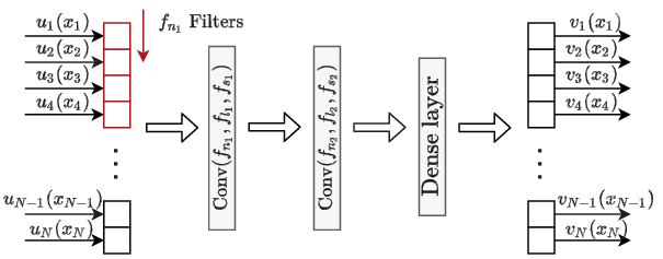
In this paper, for the sake of reducing the training complexity of the additional NN FN, we remove the max-pooling layer and simplify the CNN to have only two convolutional layers and one dense layer. The convolutional layer explores the features of the NN FN input message $u_{i}(x_{i})$. The dense layer is appended to process the features and then delivers the output to the VNs. As shown in Fig. 4, the first convolutional layer has $f_{n_{1}}$ filters and each filter has a size of $f_{l_{1}}$, where $f_{l_{1}}$ indicates that $f_{l_{1}}$ messages are considered by the filter during each convolutional step. Let $f_{s_{1}}$ denote the stride of the sliding window in the first convolutional layer. With the attachment of zero padding, the output dimension of the first convolutional layer reduces to $\lceil N/f_{s_{1}}\rceil$. The filter convolves with the messages from $u_{1}(x_{1})$ to $u_{N}(x_{N})$ to compensate any detrimental effect in the message passing that may degrade the detection performance. A similar operation of filtering is performed in the second convolutional layer which has a corresponding hyper-parameter set of $(f_{n_{2}},f_{l_{2}},f_{s_{2}})$. The output of the convolutional layer is sent to the dense layer to combine and process the filters’ results before delivering the messages to the VNs. The dense layer processes all the filters’ results and outputs the message $v_{i}(x_{i})$ for $i\in\{1,...,N\}$. The negative of a rectified linear activation function (ReLU) is used as the activation function in the dense layer [35]. During each iteration, the CNN has initial weights and biases randomly generated from a truncated normal distribution with a standard deviation of $\sigma_{\text{CNN}_{1}}$ and $\sigma_{\text{CNN}_{2}}$ for the first and second CNN layers, respectively. For each iteration, messages $u_{i}(x_{i})$ will be updated by using (9) then passed to the CNN. Messages are sent back from the CNN to join the APPs accumulation according to (11). By unfolding the FG including the NN FN to an NN system with multiple layers, the overall detector can be trained and optimized.

A loss function in an NN training is defined as the errors between the ground truth label and the estimated output. The cross-entropy loss function has been widely used for the classification problems [36] to minimize the errors between two probability distributions. By considering the BPSK constellation, we define $\hat{\mathcal{D}}_{i}^{m}(x_{i})$ as the LLR of the VN $x_{i}$ at the $m$-th iteration and $m_{max}$ as the maximum number of iterations of DL-SPDA. The cross-entropy function can be defined as $\mathcal{F}_{ce}(\bm{\mathcal{D}},\bm{\hat{\mathcal{D}}}^{m})=-\frac{1}{N}\sum_{i=1}^{N}\big(\mathcal{D}_{x_{i}}\text{log}(\frac{1}{1+e^{-\hat{\mathcal{D}}^{m}_{x_{i}}}})+(1-\mathcal{D}_{x_{i}})\text{log}(1-\frac{1}{1+e^{-\hat{\mathcal{D}}^{m}_{x_{i}}}})\big)$, where $\bm{\mathcal{D}}$ is the ground-truth label of the transmitted bits. The multi-loss function introduced in [25] and [37] can also be setup to train the tuneable parameters in the FG, which includes the tuneable weights in (8) and the weights and biases introduced in the CNN. The final loss function for training the NN is then given by:

where $\gamma<1$ is a discount factor to adjust the loss at each iteration. During the training phase, a batch of random transmitted symbols over a range of SNRs is generated as the samples to train the NN. Once the NN is fully trained, the DL-SPDA can be employed to the Turbo equalization receiver to perform as an ISI detector by exchanging the extrinsic information with the decoder. The extrinsic information from the decoder is passed to the ISI-detector without further tuning the parameters in the NN.

We have introduced the proposed DL-SPDA in Section III.A, where the FG is modified by connecting an NN FN and the message updating rule is changed accordingly. However, in our training phase, we have not considered the extrinsic information passed from the specific decoder. In other words, the extrinsic information to be conveyed to the DL-SPDA at the $\rho$-th iteration of the Turbo equalization is assumed to be an all-zero sequence, i.e. $\mathbf{\Theta}^{\rho}$ = $\mathbf{0}$. It can be observed that the DL-SPDA is optimized in the sense of ML detection. Nevertheless, it is well-known that the maximum a posterior (MAP) detection outperforms the ML detection for coded systems. Therefore, we propose a compatible training technique which considers the extrinsic information from the decoder.

Inspired by the training technique introduced in [28], we are motivated to deliver the expected distribution of the extrinsic information from the decoder to the NN by assuming that the extrinsic information follows a consistent Gaussian distribution [38], where the mean and variance can be computed from the inverse $J$-function as introduced in [29]. Note that in [28], the DNN treats the extrinsic information from the decoder as separate input neurons to the NN, i.e., the channel information and the extrinsic information from the decoder are fed into the NN separately. However, this largely increases the number of neurons in the NN and overloads the training process of the whole NN. Therefore, we propose to combine the LLRs of the channel information and the extrinsic information before sending the LLRs to the DL-SPDA, such that the DL-SPDA uses the combined information for further training.

Let $\mathbf{\Psi}^{(\cdot)}$ and $\mathbf{\Upsilon}^{(\cdot)}$ be the LLR realizations for the channel information and the extrinsic information to be passed to the detector, respectively. Note that the DL-SPDA accepts both $\mathbf{\Psi}^{(\cdot)}$ and $\mathbf{\Upsilon}^{(\cdot)}$ as the inputs. Each realization of the channel information $\mathbf{\Psi}^{(\cdot)}$ can be generated by transmitting a known data sequence $\mathbf{x}$. On the other hand, to generate the extrinsic information $\mathbf{\Upsilon}^{(\cdot)}$, we adopt the idea from the previous work in [28]. We assume that the extrinsic information $\mathbf{\Theta}^{\rho}$ follows a consistent Gaussian probability density function, i.e., $\mathbf{\Theta}_{i}^{\rho}\sim\mathcal{N}\big((-1)^{x_{i}}\sigma_{E}^{2}/2,\sigma_{E}^{2}\big)$ for $i\in\{1,...N\}$, where the variance $\sigma_{E}^{2}$ can be computed by using the inverse $J$-function [29], given the mutual information $\mathcal{M}(\mathbf{\Theta}^{\rho},\mathbf{x})$ between the extrinsic information $\mathbf{\Theta}^{\rho}$ and the transmitted sequence $\mathbf{x}$. To maintain the generality of the NN, we assume that the mutual information $\mathcal{M}(\mathbf{\Theta}^{\rho},\mathbf{x}))$ is uniformly ranged between $[0,1]$. In practice, it is sufficient to consider only a set of mutual information $\Omega=\{0,1/(|\Omega|-1),...,1\}$, where $|\Omega|$ is the cardinality of $\Omega$. Thus, a set of variances can be then determined as $\Xi=\{J^{-1}(\partial),\ \text{for}\ \partial\in\Omega\}$. Based on the variance set $\Xi$ and the known transmitted sequence $\mathbf{x}$ in the training phase, we are able to randomly generate a realization of the LLR sequence $\mathbf{\Upsilon}^{(\cdot)}_{i}\sim\mathcal{N}\big((-1)^{x_{i}}\sigma_{E}^{2}/2,\sigma_{E}^{2}\big)$, for $i\in\{1,...,N\}$.

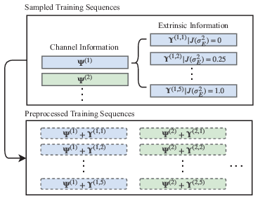
Fig. 5 illustrates the concept of the compatible training technique to improve the compatibility of the DL-SPDA in the sense of Turbo equalization, where the process is divided into two stages, namely the generation stage and the preprocessing stage. In Fig. 5, as an example, $\Omega$ is set to be $\Omega=\{0,0.25,0.5,0.75,1\}$ and one LLR realization of the extrinsic information is randomly sampled by a specific variance $\sigma_{E}^{2}\in\Xi$ for each realization of the channel information. Note that during the training phase, based on each variance $\sigma^{2}_{E}\in\Xi$, a factor $\mathcal{V}$ can be preset so that $\mathcal{V}$ realizations of the extrinsic information $\mathbf{\Upsilon}^{(\cdot)}$ are randomly sampled based on one realization of the channel information. This results in that $\mathcal{V}\times|\Omega|$ realizations of the extrinsic information will be randomly sampled based on one realization of the channel information. We call the stage above as the generation stage.

As for the preprocessing stage, we combine the extrinsic information and the channel information. Specifically, let $\mathbf{\Upsilon}^{(i,j)}$ be the $j$-th realization of the extrinsic information for the $i$-th realization of the channel information $\mathbf{\Psi}^{(i)}$, for $j\in\{1,...,\mathcal{V}\times|\Omega|\}$. The message that is passed to the VNs is the combined information sequence, where the elements in $\mathbf{\Psi}^{(i)}$ and $\mathbf{\Upsilon}^{(i,j)}$ are simply added together. As Fig. 5 demonstrated, each $i$-th realization of the channel information is separately added by the sampled extrinsic information $\mathbf{\Upsilon}^{(i,j)}$ for $j\in\{1,...,1\times|\Omega|\}$. After all the realizations have been preprocessed, the batch of sequences are fed into the NN for further training.

It can be seen that compared to the training method in Section III.B, the compatible training technique includes two more stages for processing. This indicates that the input training sequences $\{\mathbf{\Psi}^{(1)}+\mathbf{0},\mathbf{\Psi}^{(2)}+\mathbf{0},...\}$ in the previous sections are now changed to $\{\mathbf{\Psi}^{(1)}+\mathbf{\Upsilon}^{(1,1)},...,\mathbf{\Psi}^{(1)}+\mathbf{\Upsilon}^{(1,|\Omega|)},\mathbf{\Psi}^{(2)}+\mathbf{\Upsilon}^{(2,1)},...\}$. These two stages are the preprocessing of the NN training. It should be noted that the preprocessing does not add any extra input neurons to the NN while it provides the priori information for the training. Therefore, a better error performance can be expected for the DL-SPDA with the compatible training than that without the compatible training.

To begin with, we start from the ML estimation of the uncoded FTN system. Let us consider that the error sequence $\mathbf{e}$ has a Hamming error weight $w$. Therefore, it is obvious that there are in total $\mathcal{A}=\binom{N}{w}2^{w}$ combinations for $\mathbf{e}$. For the convenience of notation, we use $\mathbf{e}^{(w,j)}\in\mathcal{S}^{(N\times 1)}$ to denote a specific error sequence $\mathbf{e}$ with a Hamming error weight $w$, where $j\in\{1,...,\mathcal{A}\}$ indicates the $j$-th instance of all possible combinations of $\mathbf{e}$. Then, based on Lemma 1, the BER $P_{b}$ can be upper-bounded by applying the union bound [39], such as:

where

is the well-known Q-function [39].

We now consider the convolutionally encoded FTN system, where a uniform interleaver is assumed to be applied between the convolutional encoder and the BPSK modulator. Suppose a rate-$R$ binary terminated convolutional code (CC) $\mathcal{C}^{\prime}$ is utilized. We define $K_{b}$ bit streams as the encoder’s inputs and $N_{b}$ bit streams as outputs, i.e., $R=K_{b}/N_{b}$. According to (13), the BER performance can be estimated by considering all possible error sequences, i.e., the distance spectrum. However, conventional methods, which assume that the all-zero sequence is transmitted, to estimate the BER performance of CC over AWGN channels are not applicable [39]. This is because the Euclidean distance between coded FTN signals can be different even for error sequences with the same Hamming error weight [41]. For the ease of presentation, we refer to the error sequence $\mathbf{e}=\mathbf{x}-\mathbf{x}^{\prime}$ after the FTN modulation as the FTN error sequence, and refer to the binary error vector of the difference between two legitimate CC codewords as the CC error sequence. It is obvious that given the pair of CC codewords, the FTN error sequence and CC error sequence share the same Hammming error weight. Therefore, we aim to list all the possible CC error sequences and estimate the BER according to the corresponding FTN error sequences.

In the following, we consider that only a single error event is occurred over the CC trellis. Note that this simplification is widely considered in the literature [39]. Therefore, we intend to find out all the possible legitimate FTN error sequences that are induced by a single error event in the CC trellis. Without loss of generality, we consider CC codewords with information bit length $K^{\prime}$, which is long enough to contain all the possible codewords covering the CC error events with a relatively small Hamming error weight $w$. Define $\mathbf{c},\mathbf{c}^{\prime}\in\mathcal{C}^{\prime}$ as the instances of the $2^{K^{\prime}}$ legitimate codeword. By listing all the possible codewords, we are able to find the CC error sequences corresponding to each single error event $\varepsilon$ and $\mathbf{c}$. We use $U(\mathbf{c},\varepsilon)=\{\varepsilon|\mathcal{I}_{\varepsilon}=i,\mathcal{L}_{\varepsilon}=l,\mathcal{W}_{\varepsilon}=w\}$ to denote the set of possible single error events for a legitimate codeword $\mathbf{c}$, where each error event $\varepsilon$ in $U(\mathbf{c},\varepsilon)$ has an event error length $\mathcal{L}_{\varepsilon}=l$ and the corresponding CC error sequence has Hamming error weight $\mathcal{W}_{\varepsilon}=w$ between $\mathbf{c}$ and $\mathbf{c}^{\prime}$, corresponding to $\mathcal{I}_{\varepsilon}=i$ different information bits.

As a uniform interleaver is assumed to be employed between the convolutional encoder and the FTN modulator, each possible FTN error sequence corresponding to the CC error sequence is therefore, equally likely to be considered. Define $\mathbf{e}^{(w,o)}|\varepsilon$ as the $o$-th legitimate FTN error sequence with a Hamming error weight $w$ for a given CC event error $\varepsilon$ and $\mathcal{A}_{\varepsilon}$ as the total number of legitimate FTN error sequences for a given CC error event $\varepsilon$. The BER for the convolutionally encoded FTN system can now be upper bounded by:

It can be seen that the denominator part in (15) is due to the assumptions of binary symmetric inputs of the convolutional encoder and the employment of the uniform interleaver between the convolutional encoder and the FTN signaling.

With the analysis of the finite length coded FTN system which considers full ISI taps, we can now investigate the error performance for the ML estimate when a finite number of ISI taps $L_{E}<L$ is considered by the detector. As in the previous section, we firstly consider the case of uncoded finite-taps FTN signaling. Following [30] and Definition 2, we intend to find the error probability $P_{\mathbf{e}}^{{}^{\prime}}$ under the condition that a finite number of ISI responses is considered at the receiver, which is equivalent of finding the probability of $P(\text{Re}\big\{\mathbf{e}^{\text{H}}\bm{\eta}+\mathbf{e}^{\text{H}}(\mathbf{G}-\mathbf{F})\mathbf{x}\big\}>E_{b}d^{2}_{\text{ope}}(\mathbf{e}))$. It can be seen that $\mathbf{e}^{\text{H}}(\mathbf{G}-\mathbf{F})\mathbf{x}$ represents the influence of the residual ISI that is not considered by the matrix $\mathbf{F}$. Define the term $\wp\triangleq\text{Re}\big\{\mathbf{e}^{\text{H}}\bm{\eta}+\mathbf{e}^{\text{H}}(\mathbf{G}-\mathbf{F})\mathbf{x}\big\}$. In particular, the term $\wp$ can be modeled as a Gaussian variable according to the central limit theorem and it can be shown that $\mathbb{E}[\wp]=0$ and the variance $\mathbb{E}[\wp\wp^{\rm{H}}]=N_{0}E_{b}d^{2}(\mathbf{e})+2E_{b}\sigma^{2}_{\text{R},\mathbf{e}}$, where $\sigma^{2}_{\text{R},\mathbf{e}}$ refers to the variance of the term $\mathbf{e}^{\text{H}}(\mathbf{G}-\mathbf{F})\mathbf{x}$ induced by the residual ISI taps for a given error sequence $\mathbf{e}$. In specific, we have $\sigma^{2}_{\text{R},\mathbf{e}}=\frac{1}{2E_{b}}\mathbb{E}[\mathbf{x}^{\text{H}}(\mathbf{G}-\mathbf{F})\mathbf{e}\mathbf{e}^{\text{H}}(\mathbf{G}-\mathbf{F})^{\text{H}}\mathbf{x}]$ [30]. Based on the derivations in [30], the error probability for an ML detection if finite taps of ISI responses are considered by the detector is approximated by the following lemma:

Finding the expectation over all the possible transmitted sequence $\mathbf{x}$ for a given $\mathbf{e}$ can be computationally prohibitive. In the following, we introduce a theorem that obtains the lower bound $\sigma^{2}_{\text{R}_{L},\mathbf{e}}$ for $\sigma^{2}_{\text{R},\mathbf{e}}$.

Based on Theorem 1, we further obtain the following corollary.

Based on Lemma 2, we are able to derive the analytical BERs for the coded FTN signaling, where the ML detector considers finite ISI responses. As previously described, $\sigma_{{\text{R},\mathbf{e}}}^{2}$ is derived by computing the expectation over all the possible transmitted sequences $\mathbf{x}$, while $\sigma_{{\text{R}_{L},\mathbf{e}}}^{2}$ is determined based on the error sequence $\mathbf{e}$. It is reasonable to employ $\sigma_{{\text{R}_{L},\mathbf{e}}}^{2}$ to estimate the error probability for $\mathbf{e}$. Moreover, to simplify the computation complexity, the distance spectrum of the FTN signaling can be searched based on the FTN error events [12, 42, 43]. For instance, given a CC error event $\varepsilon$ and a Hamming error weight $w$, let $\Big\{\big(D_{1_{\varepsilon}},d^{2}(\mathbf{\tilde{e}}^{(w,1)}|\varepsilon),d^{2}_{\text{ope}}(\mathbf{\tilde{e}}^{(w,1)}|\varepsilon)\big),...,\big(D_{M_{\varepsilon}},d^{2}(\mathbf{\tilde{e}}^{(w,M)}|\varepsilon),,d^{2}_{\text{ope}}(\mathbf{\tilde{e}}^{(w,M)}|\varepsilon)\big)\Big\}$ be the distance spectrum for the CC error event $\varepsilon$, where $D_{o_{\varepsilon}}$ denotes the corresponding number of error sequences which have the same Euclidean and operative distance as $\mathbf{\tilde{e}}^{(w,o)}$ and $M_{\varepsilon}$ denotes the total number of considered error sequences. According to Corollary 1, any two error sequences with the same Euclidean distance and operative Euclidean distance have the same values of $\sigma_{\text{R}_{L},\mathbf{e}}^{2}$. Therefore, the BER for a convolutionally encoded FTN system with a finite number of ISI responses can be approximated by:

Note that the analytical BER in (IV-B) is an approximation of the real BER due to the use of the lower bound of $\sigma^{2}_{\text{R},\mathbf{e}}$. As will be shown in the numerical results, in a high SNR region, using $\sigma_{{\text{R}_{L},\mathbf{e}}}^{2}$ has achieved a close estimate to the error performance of the ML detection and decoding. More importantly, the lower bound $\sigma_{{\text{R}_{L},\mathbf{e}}}^{2}$ becomes closer to $\sigma_{{\text{R},\mathbf{e}}}^{2}$, if the influence of the residual ISI tends to be insignificant. Furthermore, (IV-B) demonstrates that the ML performance is restricted by the number of ISI taps considered by the detection algorithm. If full-taps are considered, then $d^{2}_{\text{ope}(\mathbf{e})}$ is identical to $d^{2}(\mathbf{e})$ and the residual ISI term will vanish. In the following numerical results, we will show that when finite taps are considered by the conventional SPDA, the performance is limited by the residual ISI taps and an error floor occurs in a high SNR region when the noise has less impact to the performance than the residual ISI. On the other hand, simulation results show that the performance of the DL-SPDA approaches to that of the ML detection and decoding which is consistent with our analysis.

In this section, we evaluate the performance of the proposed DL-SPDA scheme for convolutionally encoded FTN systems. Without loss of generality, we consider the coded FTN systems with $\tau=0.5$ and $\tau=0.6$, respectively, where the (7, 5) 4-state rate-1/2 non-recursive CC is used. At the receiver, Turbo equalization is performed, where the extrinsic information is exchanged between the DL-SPDA detector and the BCJR decoder for CC. Compatible training method is applied to the DL-SPDA.

To have a fair comparison, we also perform the SPDA [19] and the channel shortening (CS) method as proposed in [44]. Furthermore, truncated-BCJR detection algorithm [45] for FTN detection is also evaluated to demonstrate the accuracy of the analytical bound, i.e., (15) and (IV-B), when a limited number of ISI taps is considered by the detection algorithm. Note that, in order to improve the error perforamnce, the BCJR algorithm usually requires a terminated trellis [39]. Therefore, in our simulation, we intentionally transmit additional symbols to terminate the ISI trellis. Specifically, four additional code symbols are transmitted for the BCJR decoder for CC, while $2\times L_{E}$ additional symbols are transmitted for the truncated-BCJR algorithm. The analytical BER of a specific code rate $R$ is summed over the CC minimum Hamming distance $w=d_{\text{min}}=5$ to a Hamming error weight 8 and the approximate full-taps BERs consider $L=11$ ISI responses.

The corresponding code rate $R$ with the implementation of the truncated-BCJR detection algorithm and BCJR decoding algorithm is provided in the figures for reference, which is also used for the calculation of analytical BERs. In this paper, the hyper-parameters to train the NN system are shown in Table I.

Note that for a BPSK modulation, the LLR values can be computed by $u_{i}(x_{i})$ for $i\in\{1,...,N\}$, where the LLR values serve as the input of the CNN FN.

The error performance of various detection algorithms for the FTN systems is shown in Figs. 6, 7, 8 and 9. Let $\rho_{max}$ indicate the number of iterations of the Turbo equalization and $L_{E}$ denotes the number of truncated ISI taps. DL-SPDA($\rho_{max}$, $L_{E}$) indicates the proposed DL-SPDA detection method, and BCJR($\rho_{max}$, $L_{E}$) refers to the corresponding truncated-BCJR detection algorithm [45]. Both DL-SPDA and SPDA utilize 6 iterations for updating the messages. Unless specially notified, we compare the error performance at BER $\approx 1\times 10^{-5}$.

In Fig. 6, the comparison between analytical bound and the proposed algorithm of an FTN system with $\tau=0.6$ and $N=250$ is shown, where we can observe that DL-SPDA(15, 3) has achieved a closed performance to the analytical bound with a code rate $R=0.492$. Furthermore, we demonstrate the correctness of the derived analytical BERs by performing BCJR(15, 7), where the error performance has a close match to the analytical BERs with a code rate $R=0.466$.

In Fig. 7, the simulation results of an FTN system with $\tau=0.6$ and $N=250$ are provided. It can be seen that DL-SPDA(15, 3) provides 0.35 dB gain compared to the SPDA(15, 3) at a BER = $3.2\times 10^{-6}$, where both algorithms consider the same number of ISI taps in the original Tanner graph. This is due to the fact that after the off-line training, the DL-SPDA algorithm has “learned” the residual ISIs which are not considered by the original FG. Meanwhile, the error performance of CS(15, 6) is also provided in Fig. 7. As observed from the figure, both DL-SPDA(15, 3) and CS(15, 6) achieve almost the same error performance that is close to the analytical bound. However, the proposed DL-SPDA requires less complexity, which will be discussed in Section V.B.

In Fig. 8, we provide the comparison between the analytical BERs for finite-length finite-tap ML estimate and the simulation results for coded FTN signaling. The truncated-BCJR detection algorithm and BCJR decoding algorithm are employed. The codeword length is $N=250$ and $\tau=0.6$. In order to demonstrate that an NN FN is capable to capture the interference characteristics throughout the off-line training, we set the DL-SPDA to consider 2 ISI taps based on the Tanner graph and we expect the NN FN learns all the ISI taps leading to an error performance that approachs the analytical bound. The simulation results in the low SNR region show close performances to the analytical BERs. Since a lower bound for $\sigma^{2}_{\text{R},\mathbf{e}}$ is implemented as in (IV-B), the BERs are slightly lower than the simulation results of the BCJR algorithm in the high SNR region, when 2 taps are considered by the truncated-BCJR algorithm. It can be seen that the SPDA(15, 2) has an error floor at a BER = $2\times 10^{-7}$ due to the insufficient considered ISI taps, while with the help of the concatenated neural network, DL-SPDA(15, 2) shows a promising performance with no noticeable error floor at a BER $<10^{-7}$.

Fig. 9 depicts the error performance of an FTN system with a more difficult ISI, e.g. $N=250$ and $\tau=0.5$. The DL-SPDA(15, 3) outperforms SPDA(15, 3) by 0.75 dB at a BER = $2.5\times 10^{-5}$. We observe that DL-SPDA(15, 3) has a close performance to the CS(15, 6). From Fig. 9, we observe that for conventional SPDA, the performance is poor due to the strong ISI and the short codeword length. On the other hand, DL-SPDA can compensate the strong correlation that exists in the detecting messages and help the detector converges to a better performance.

In Fig. 10, the normalized average training loss for every $10^{3}$ training batches for an FTN signaling of $\tau=0.5$ and $N=250$ with the DL-SPDA(15, 3) is shown. Define $\xi^{a}_{\text{avg}}$ as the average loss from $(a-1)\times 5\times 10^{3}$ to $a\times 5\times 10^{3}$ batches ($\xi^{0}_{\text{avg}}=1$) and define $\xi^{a}_{\text{cg}}=|(\xi^{a}_{\text{avg}}-\xi^{a-1}_{\text{avg}})/\xi^{a-1}_{\text{avg}}|$ as the percentage of the absolute change on the average loss $(\xi^{0}_{\text{cg}}=0)$, where $a\in\mathbb{Z}$. Define that a stable performance of the training is reached after $a\times 5\times 10^{3}$ batches, if $\xi^{a^{\prime}}_{\text{cg}}<0.1$ for any integer $a^{\prime}>a$. From Fig. 10, we can see that the training phase of the proposed algorithm takes roughly $180\times 70000$ = $1.26\times 10^{7}$ training samples to converge to a relative stable performance. Benefited from the derived FG and simplified NN model, this number of training samples is much smaller than the conventional NN decoders which generally need more than $2^{K}$ training samples to converge to a good performance.

Previous simulation results demonstrate the potential BER performance gain that can be acquired by the proposed DL-SPDA based on the structure of conventional SPDA. In this section, we discuss the computational complexity of the proposed DL-SPDA. We mainly compare the computational complexity with the SPDA and the maximum a posteriror (MAP) detection algorithm, i.e., log-BCJR algorithm [46]. Compared to the conventional SPDA, DL-SPDA has extra computational complexity introduced by the additional neural network function node. The multiplicative weights attached to the interference node $I_{i,j}\{x_{i},x_{j}\}$ and the interference node itself can be considered as one parameter during the message computation. Therefore, no additional complexity is added by the multiplicative weights of the messages $p_{j,i}(x_{j})$ in Section III. In Table II, we show the approximated computational complexity comparison by the number of addition and look-up table accesses, where the operations of comparison, multiplication and non-linear process are assumed to be executed through the look-up table access. According to [46], the log-MAP algorithm has a computational complexity that grows exponentionally with the considered number of ISI taps. Comparatively, the SPDA has a linear complexity with the number of ISI per message-passing iteration. In Table II, the extra computation complexity that the DL-SPDA requires on top of the SPDA is shown. For the additions, there are mainly two processes in the DL-SPDA, which are the extra message $v_{i}(x_{i})$ at VN $x_{i}$ and the process of the neural function node, respectively. Similar to the additions, the processes of the convolutional layer, the ReLu non-linear activation function and the fully connected layer are considered by the look-up table accesses. In our numerical results, with 6 iterations, DL-SPDA(15, 3) has approximately $2.4\times 10^{5}$ additions and $1.0\times 10^{5}$ look-up table accesses. Comparatively, CS(15, 6) performs linear filtering and the BCJR algorithm. In specific, the BCJR algorithm requires $2.42\times 10^{5}$ additions and $1.59\times 10^{5}$ look-up table accesses, which is 60$\%$ more than the DL-SPDA algorithm. Since FTN signaling theoretically introduces infinite number of ISI responses, the difference of computational complexity becomes more significant as more ISI responses are considered by the log-MAP detection algorithm. More importantly, the proposed algorithm offers the flexility of designing the NN, where the complexity of the proposed algorithm might be further mitigated with advanced NN designs.

References

- [1] B. Liu, S. Li, Y. Xie, and J. Yuan, “Deep learning assisted sum-product detection algorithm for faster-than-Nyquist signaling,” in IEEE Inf. Theory Workshop (ITW), Aug. 2019, pp. 1–5.
- [2] J. E. Mazo, “Faster-than-Nyquist signaling,” Bell Syst. Tech. J., vol. 54, no. 8, pp. 1451–1462, Oct. 1975.
- [3] J. B. Anderson, F. Rusek, and V. Owall, “Faster-Than-Nyquist Signaling,” Proc. IEEE, vol. 101, no. 8, pp. 1817–1830, Aug. 2013.
- [4] S. Li, B. Bai, J. Zhou, Q. He, and Q. Li, “Superposition coded modulation based faster-than-Nyquist signaling,” Wireless Commun. Mobile Comput., vol. 2018, 2018.
- [5] F. Rusek and J. B. Anderson, “Constrained capacities for faster-than-Nyquist signaling,” IEEE Trans. Inf. Theory, vol. 55, no. 2, pp. 764–775, Feb. 2009.
- [6] A. Piemontese, A. Modenini, G. Colavolpe, and N. S. Alagha, “Improving the spectral efficiency of nonlinear satellite systems through time-frequency packing and advanced receiver processing,” IEEE Trans. Commun., vol. 61, no. 8, pp. 3404–3412, Aug. 2013.
- [7] B. Lee, J. Kim, H. Lee, B. Shim, Y. Kim, and J. Lee, “Towards faster-than-Nyquist transmission for beyond 5G wireless communications,” in Proc. IEEE Intern. Commun. Conf., May. 2019, pp. 1–6.
- [8] W. Yuan, N. Wu, Q. Guo, D. W. K. Ng, J. Yuan, and L. Hanzo, “Iterative joint channel estimation, user activity tracking, and data detection for FTN-NOMA systems supporting random access,” IEEE Trans. Commun., vol. 68, no. 5, pp. 2963–2977, Feb. 2020.
- [9] C. Douillard, M. Jezequel, C. Berrou, D. Electronique, A. Picart, P. Didier, and A. Glavieux, “Iterative correction of intersymbol interference: Turbo-equalization,” European Trans. Telecommun., vol. 6, no. 5, pp. 507–511, Sep. 1995.
- [10] M. Tuchler, R. Koetter, and A. C. Singer, “Turbo equalization: Principles and new results,” IEEE Trans. Commun., vol. 50, no. 5, pp. 754–767, May. 2002.
- [11] W. Yuan, N. Wu, A. Zhang, X. Huang, Y. Li, and L. Hanzo, “Iterative receiver design for FTN signaling aided sparse code multiple access,” IEEE Trans. Wireless Commun., Nov. 2019.
- [12] S. Li, B. Bai, J. Zhou, P. Chen, and Z. Yu, “Reduced-complexity equalization for faster-than-Nyquist signaling: New methods based on Ungerboeck observation model,” IEEE Trans. Commun., vol. 66, no. 3, pp. 1190–1204, Mar. 2018.
- [13] C. Fragouli, N. Seshadri, and W. Turin, “Reduced-trellis equalization using the M-BCJR algorithm,” Wireless Commun. Mobile Comp., vol. 1, no. 4, pp. 397–406, Jul. 2001.
- [14] D. Fertonani, A. Barbieri, and G. Colavolpe, “Reduced-complexity BCJR algorithm for turbo equalization,” IEEE Trans. Commun., vol. 55, no. 12, pp. 2279–2287, Dec. 2007.
- [15] G. Ungerboeck, “Adaptive maximum-likelihood receiver for carrier-modulated data-transmission systems,” IEEE Trans. Commun., vol. 22, no. 5, pp. 624–636, May. 1974.
- [16] F. R. Kschischang, B. J. Frey, and H. . Loeliger, “Factor graphs and the sum-product algorithm,” IEEE Trans. Inf. Theory, vol. 47, no. 2, pp. 498–519, Feb. 2001.
- [17] T. J. Richardson, M. A. Shokrollahi, and R. L. Urbanke, “Design of capacity-approaching irregular low-density parity-check codes,” IEEE Trans. Inf. Theory, vol. 47, no. 2, pp. 619–637, Feb. 2001.
- [18] D. L. Donoho, A. Maleki, and A. Montanari, “Message passing algorithms for compressed sensing,” CoRR, vol. abs/0907.3574, 2009. [Online]. Available: http://arxiv.org/abs/0907.3574
- [19] G. Colavolpe, D. Fertonani, and A. Piemontese, “SISO detection over linear channels with linear complexity in the number of interferers,” IEEE J. Sel. Topics Signal Process., vol. 5, no. 8, pp. 1475–1485, Dec. 2011.
- [20] T. Faghani, A. Shojaeifard, K. Wong, and A. H. Aghvami, “Deep learning-based decision region for MIMO detection,” in 2019 IEEE 30th Ann. Int. Symp. Personal, Indoor Mobile Radio Commun. (PIMRC), Sep. 2019, pp. 1–5.
- [21] Q. Huang, C. Zhao, M. Jiang, X. Li, and J. Liang, “A novel OFDM equalizer for large doppler shift channel through deep learning,” in 2019 IEEE 90th Veh. Tech. Conf. (VTC2019-Fall), Sep. 2019, pp. 1–5.
- [22] X. Jin and H. Kim, “Parallel deep learning detection network in the MIMO channel,” IEEE Commun. Lett., pp. 1–1, Oct. 2019.
- [23] A. Abotabl, J. H. Bae, and K. Song, “Offset min-sum optimization for general decoding scheduling: A deep learning approach,” in 2019 IEEE 90th Veh. Tech. Conf. (VTC2019-Fall), Sep. 2019, pp. 1–5.
- [24] A. Felix, S. Cammerer, S. Dörner, J. Hoydis, and S. Ten Brink, “OFDM-autoencoder for end-to-end learning of communications systems,” in 2018 IEEE 19th Int. Workshop Signal Proc. Advances Wireless Commun. (SPAWC), 2018, pp. 1–5.
- [25] E. Nachmani, E. Marciano, L. Lugosch, W. J. Gross, D. Burshtein, and Y. Be’ery, “Deep learning methods for improved decoding of linear codes,” IEEE J. Sel. Topics Signal Process., vol. 12, no. 1, pp. 119–131, Feb. 2018.
- [26] M. Lian, F. Carpi, C. Häger, and H. D. Pfister, “Learned belief-propagation decoding with simple scaling and SNR adaptation,” CoRR, vol. abs/1901.08621, 2019. [Online]. Available: http://arxiv.org/abs/1901.08621
- [27] T. Gruber, S. Cammerer, J. Hoydis, and S. ten Brink, “On deep learning-based channel decoding,” CoRR, vol. abs/1701.07738, 2017. [Online]. Available: http://arxiv.org/abs/1701.07738
- [28] T. Koike-Akino, Y. Wang, D. S. Millar, and K. Kojima, “Neural turbo equalization to mitigate fiber nonlinearity,” in European Conf. Optical Comm. (ECOC), Sep. 2019.
- [29] S. ten Brink, “Convergence behavior of iteratively decoded parallel concatenated codes,” IEEE Trans. Commun., vol. 49, no. 10, pp. 1727–1737, Oct. 2001.
- [30] S. Li, W. Yuan, J. Yuan, B. Bai, D. Wing Kwan Ng, and L. Hanzo, “Time-domain vs. frequency-domain equalization for FTN signaling,” IEEE Trans. Veh. Technol., vol. 69, no. 8, pp. 9174–9179, Jun. 2020.
- [31] T. Richardson and R. Urbanke, Modern Coding Theory. USA: Cambridge University Press, 2008.
- [32] Y. LeCun, B. Boser, J. S. Denker, D. Henderson, R. E. Howard, W. Hubbard, and L. D. Jackel, “Backpropagation applied to handwritten zip code recognition,” Neural Comp., vol. 1, no. 4, pp. 541–551, Dec. 1989.
- [33] C. Fan, X. Yuan, and Y. Zhang, “CNN-based signal detection for banded linear systems,” IEEE Trans. Wireless Commun., vol. 18, no. 9, pp. 4394–4407, Sep. 2019.
- [34] T. Wu, “CNN and RNN-based deep learning methods for digital signal demodulation,” in Proc. Int. Conf. Image, Video Signal Process., ser. IVSP 2019. New York, NY, USA: ACM, 2019, pp. 122–127.
- [35] V. Nair and G. E. Hinton, “Rectified linear units improve restricted boltzmann machines,” in Proc. Int. Conf. Machine Learning, ser. ICML’10. USA: Omnipress, 2010, pp. 807–814.
- [36] I. Goodfellow, Y. Bengio, and A. Courville, Deep Learning. The MIT Press, 2016.
- [37] A. Bennatan, Y. Choukroun, and P. Kisilev, “Deep learning for decoding of linear codes - A syndrome-based approach,” arXiv e-prints, p. arXiv:1802.04741, Feb. 2018.
- [38] J. B. Anderson and M. Zeinali, “Best rate 1/2 convolutional codes for turbo equalization with severe ISI,” in Proc. IEEE Intern. Sympos. Inf. Theory, Jul. 2012, pp. 2366–2370.
- [39] S. Lin and D. J. Costello, Error Control Coding, Second Edition. USA: Prentice-Hall, Inc., 2004.
- [40] M. Loncar and F. Rusek, “On reduced-complexity equalization based on Ungerboeck and Forney observation models,” IEEE Trans. Signal Process., vol. 56, no. 8, pp. 3784–3789, Aug. 2008.
- [41] S. Li, J. Yuan, B. Bai, and N. Benvenuto, “Code-based channel shortening for faster-than-Nyquist signaling: Reduced-complexity detection and code design,” IEEE Trans. Commun., vol. 68, no. 7, pp. 3996–4011, Apr. 2020.
- [42] Jing Li, K. R. Narayanan, and C. N. Georghiades, “An efficient algorithm to compute the Euclidean distance spectrum of a general intersymbol interference channel and its applications,” IEEE Trans. Commun., vol. 52, no. 12, pp. 2041–2046, Dec. 2004.
- [43] X.-G. Xia, Modulated Coding for Intersymbol Interference Channels. Signal Process. and Commun., 2000.
- [44] F. Rusek and A. Prlja, “Optimal channel shortening for MIMO and ISI channels,” IEEE Trans. Wireless Commun., vol. 11, no. 2, pp. 810–818, Dec. 2012.
- [45] G. Colavolpe and A. Barbieri, “On MAP symbol detection for ISI channels using the Ungerboeck observation model,” IEEE Commun. Lett., vol. 9, no. 8, pp. 720–722, Aug. 2005.
- [46] P. Robertson, E. Villebrun, and P. Hoeher, “A comparison of optimal and sub-optimal MAP decoding algorithms operating in the log domain,” in Proc. IEEE Int. Conf. Commun., vol. 2, 1995, pp. 1009–1013.