跳到论文正文
W Papers独立论文阅读器 arXiv:2012.08032 论文正文 计算阅读时间 · 0%
引用这篇论文根据当前论文元数据生成,正式投稿前建议核对。


License: CC BY-NC-ND 4.0
arXiv:2012.08032v1 [math.OC] 15 Dec 2020

Linear Quadratic Control of Backward Stochastic Differential Equation with Partial Information Thanks: This work supported by the National Natural Science Foundations of China under Grants 61821004, 61633015, 61877062, and 61977043.

Guangchen Wang Thanks: School of Control Science and Engineering, Shandong University, Jinan 250061, PR China, E-mail: wguangchen@sdu.edu.cn    Wencan Wang Thanks: School of Control Science and Engineering, Shandong University, Jinan 250061, PR China, E-mail: wwencan@163.com    Zhiguo Yan Thanks: School of Electrical Engineering and Automation, Qilu University of Technology (Shandong Academy of Sciences), Jinan 250353, PR China, E-mail:yanzg500@sina.com

Abstract: In this paper, we study an optimal control problem of linear backward stochastic differential equation (BSDE) with quadratic cost functional under partial information. This problem is solved completely and explicitly by using a stochastic maximum principle and a decoupling technique. By using the maximum principle, a stochastic Hamiltonian system, which is a forward-backward stochastic differential equation (FBSDE) with filtering, is obtained. By decoupling the stochastic Hamiltonian system, three Riccati equations, a BSDE with filtering, and a stochastic differential equation (SDE) with filtering are derived. We then get an optimal control with a feedback representation. An explicit formula for the corresponding optimal cost is also established. As illustrative examples, we consider two special scalar-valued control problems and give some numerical simulations.

Keywords: Linear quadratic optimal control; backward stochastic differential equation; filtering; Ricatti equation; feedback representation.

Mathematics Subject Classification: 93E20, 60H10

1 Introduction

A BSDE is an Itô SDE for which a random terminal rather than an initial condition on state has been specified. Bismut [1] first introduced a linear BSDE, which is an adjoint equation of stochastic optimal control problem. Pardoux and Peng [2] extended the linear BSDE to a general case. Since then, there has been considerable attention on related topics and their applications among researchers in mathematical finance and stochastic optimal control. See for example, El Karoui et al. [3], Ma and Yong [4], Kohlmann and Zhou [5].

Since BSDE stems from stochastic control theory, it is very natural and appealing to investigate optimal control problem of BSDE. Moreover, controlled BSDE is expected to have wide and important applications in various fields, especially in mathematical finance. In financial investment, a European contingent claim ξ\xi, which is a random variable, can be thought as a contract to be guaranteed at maturity TT. Peng [6] and Dokuchaev and Zhou [7] derived local and global stochastic maximum principles of optimality for BSDEs, respectively. Linear quadratic (LQ) optimal control problems of BSDEs have also been investigated. Lim and Zhou [8] discussed an LQ control problem of BSDE with a general setting and gave a feedback representation of the optimal control. Li et al. [9] extended the results in [8] to the case with mean-field term. Huang et al. [10] and Du et al. [11] considered LQ backward mean-field games. Du and Wu [12] concerned a stackelberg game for mean field linear BSDE with quadratic cost functionals.

In this paper, we investigate an LQ control problem of BSDE with partial information, which will be referred as a stochastic backward LQ control problem. We are devoted to deriving the optimal control with a feedback representation and establishing an explicit formula for the corresponding optimal cost. Note that the mentioned papers above are concentrated on the complete information case. The motivation of studying stochastic control problems with partial information arises naturally from the area of financial economics. In a portfolio and consumption problem, let 𝔽≡{ℱt}t≥0\mathbb{F}\equiv\{\mathcal{F}_{t}\}_{t\geq 0} denote the flow of information generated by all market noises. In reality, the information available to an agent maybe less than the one produced by the market noises, that is, 𝒢t⊆ℱt\mathcal{G}_{t}\subseteq\mathcal{F}_{t}, where 𝔾≡{𝒢t}t≥0\mathbb{G}\equiv\{\mathcal{G}_{t}\}_{t\geq 0} is the information available to the agent. There are considerable literatures on related topics [13, 14, 15, 16, 17, 18]. In particular, Huang et al. [15] derived a necessary condition for optimality of BSDE with partial information and applied their results to two classes of LQ problems. Wang et al. [16] and Wang et al. [17] concerned LQ problems with partially observable information driven by FBSDE and mean field FBSDE, respectively. LQ non-zero sum stochastic differential game of BSDE is considered in Wang et al. [18]. They obtained feedback Nash equilibrium points by FBSDE and Riccati equation under asymmetric information.

Our work distinguishes itself from existing literatures in the following aspects. (i) Both the generator of dynamic system and the cost functional contain diffusion terms Z1Z_{1} and Z2Z_{2}. Moreover, our results are obtained under some usual conditions (see Assumptions A​1A1 and A​2A2 in section 2). In the literatures on this topic, diffusion terms Z1Z_{1} and Z2Z_{2} are usually assumed not to be contained into the generator (see [15], [17]), or there are some additional conditions to ensure the solvability of Riccati equation (see [16], [18]). (ii) Sufficient and necessary conditions of optimality are established, which provide an expression for optimal control via the solution of stochastic Hamiltonian system. (iii) Explicit representations for optimal control in terms of three Riccati equations, a BSDE with filtering, and an SDE with filtering are obtained, as well as the associated optimal cost. The derivation of associated Riccati equations is extremely different from [8] and [9], since the stochastic Hamiltonian system is an FBSDE with filtering. Moreover, the uniqueness and existence of solution to BSDE (3.5) is first obtained, which is important in deriving explicit representations for optimal control and associated optimal cost. (iv) Last but not least, we consider two special scalar-valued control problems of BSDEs with partial information. In the case of H=N1=0H=N_{1}=0, we obtain explicit solutions of the stochastic Hamiltonian system, as well as related Riccati equations. In the case of C2=0C_{2}=0, we give some numerical simulations to illustrate our theoretical results.

The rest of this paper is organized as follows. In Section 2, we formulate the stochastic backward LQ control problem and give some preliminary results. Section 3 aims to decouple the associated stochastic Hamiltonian system and derive some Riccati equations. In Section 4, we give explicit representations of optimal control and the associated optimal cost. Section 5 is devoted to solving two special scalar-valued control problems and giving some numerical simulations. Finally, we conclude this paper.

2 Preliminaries

Let (Ω,ℱ,𝔽,ℙ)(\Omega,\mathcal{F},\mathbb{F},\mathbb{P}) be a complete filtered probability space and let T>0T>0 be a fixed time horizon. Let {(W1​t,W2​t):0≤t≤T}\{(W_{1t},W_{2t}):0\leq t\leq T\} be a ℝ2\mathbb{R}^{2}-valued standard Wiener process, defined on (Ω,ℱ,𝔽,ℙ)(\Omega,\mathcal{F},\mathbb{F},\mathbb{P}). 𝔽≡{ℱt}t≥0\mathbb{F}\equiv\{\mathcal{F}_{t}\}_{t\geq 0} is a natural filtration of (W1,W2)(W_{1},W_{2}) augmented by all ℙ\mathbb{P}-null sets. Let ℱtβ=σ{βs, 0≤s≤t}\mathcal{F}_{t}^{\beta}=\sigma\{\beta_{s},\ 0\leq s\leq t\} be the filtration generated by a stochastic process β\beta. Let ℝn×m\mathbb{R}^{n\times m} be the set of all n×mn\times m matrices and 𝕊n\mathbb{S}^{n} be the set of all n×nn\times n symmetric matrices. For a matrix M∈ℝnM\in\mathbb{R}^{n}, let M⊤M^{\top} be its transpose. The inner product ⟨⋅,⋅⟩\langle\cdot,\cdot\rangle on ℝn×m\mathbb{R}^{n\times m} is defined by ⟨M,N⟩↦t​r​(M⊤​N)\langle M,N\rangle\mapsto tr(M^{\top}N) with an induced norm |M|=t​r​(M⊤​M)|M|=\sqrt{tr(M^{\top}M)}. In particular, we denote by 𝕊+n\mathbb{S}_{+}^{n} (𝕊^+n\widehat{\mathbb{S}}_{+}^{n}) the set of all n×nn\times n (uniformly) positive definite matrices. For any Euclidean space MM, we adopt the following notations:
ℒℱT2(Ω;M)={ζ:Ω→M|ζ\mathcal{L}_{\mathcal{F}_{T}}^{2}(\Omega;M)=\Big\{\zeta:\Omega\to M|\zeta is an ℱT\mathcal{F}_{T}-measurable random variable, 𝔼⁡[|ζ|2]<∞\mathbb{E}[|\zeta|^{2}]<\infty};
ℒ∞(0,T;M)={v:[0,T]→M|v\mathcal{L}^{\infty}(0,T;M)=\Big\{v:[0,T]\to M|v is a bounded function};
ℒℱ2(0,T;M)={v:[0,T]×Ω→M|v\mathcal{L}_{\mathcal{F}}^{2}(0,T;M)=\Big\{v:[0,T]\times\Omega\to M|v is an {ℱt}t≥0\{\mathcal{F}_{t}\}_{t\geq 0}-adapted stochastic process, 𝔼[∫0T|vt|2dt]<∞};\mathbb{E}\left[\int_{0}^{T}|v_{t}|^{2}dt\right]<\infty\Big\};
𝒮ℱ2(0,T;M)={v:[0,T]×Ω→M|v\mathcal{S}_{\mathcal{F}}^{2}(0,T;M)=\Big\{v:[0,T]\times\Omega\to M|v is an {ℱt}t≥0\{\mathcal{F}_{t}\}_{t\geq 0}-adapted stochastic process and has continuous paths, 𝔼[supt∈[0,T]|vt|2]<∞}\mathbb{E}\left[\sup_{t\in[0,T]}|v_{t}|^{2}\right]<\infty\Big\}.

Consider a controlled linear BSDE

{d​Yt=(At​Yt+Bt​vt+C1​t​Z1​t+C2​t​Z2​t)​d​t+Z1​t​d​W1​t+Z2​t​d​W2​t,t∈[0,T],YT=ζ,\left\{\begin{aligned} dY_{t}=&\big(A_{t}Y_{t}+B_{t}v_{t}+C_{1t}Z_{1t}+C_{2t}Z_{2t}\big)dt+Z_{1t}dW_{1t}+Z_{2t}dW_{2t},\quad t\in{[0,T]},\\ Y_{T}=&\ \zeta,\end{aligned}\right. (2.1)

where ζ∈LℱT2​(Ω,ℝn)\zeta\in L_{\mathcal{F}_{T}}^{2}(\Omega;\mathbb{R}^{n}) and vv, valued in ℝm\mathbb{R}^{m}, is a control process. Introduce an admissible control set
𝒱a​d[0,T]={v:[0,T]×Ω→ℝm|vis{ℱtW1}t≥0−\mathcal{V}_{ad}[0,T]=\Big\{v:[0,T]\times\Omega\to\mathbb{R}^{m}|v\ is\ \{\mathcal{F}_{t}^{W_{1}}\}_{t\geq 0}- adapted, 𝔼[∫0T|vt|2dt]<∞}.\mathbb{E}\left[\int_{0}^{T}|v_{t}|^{2}dt\right]<\infty\Big\}.
Any v∈𝒱a​d​[0,T]v\in\mathcal{V}_{ad}[0,T] is called an admissible control.
Assumption A​1A1: The coefficients of dynamic system satisfy

A,C1,C2∈ℒ∞​(0,T,ℝn×n),B∈ℒ∞​(0,T,ℝn×m).A,C_{1},C_{2}\in\mathcal{L}^{\infty}(0,T;\mathbb{R}^{n\times n}),\ B\in\mathcal{L}^{\infty}(0,T;\mathbb{R}^{n\times m}).

Under Assumption A​1A1, dynamic system (2.1) admits a unique solution pair (Y,Z1,Z2)∈𝒮ℱ2​(0,T,ℝn)×ℒℱ2​(0,T,ℝn)×ℒℱ2​(0,T,ℝn)(Y,Z_{1},Z_{2})\in\mathcal{S}_{\mathcal{F}}^{2}(0,T;\mathbb{R}^{n})\times\mathcal{L}_{\mathcal{F}}^{2}(0,T;\mathbb{R}^{n})\times\mathcal{L}_{\mathcal{F}}^{2}(0,T;\mathbb{R}^{n}), which is called the corresponding state process, for any v∈𝒱a​d​[0,T]v\in\mathcal{V}_{ad}[0,T] (see Pardoux and Peng [2], Yong and Zhou [19]). We introduce a quadratic cost functional

J⁡(v)=\displaystyle J(v)= 12​𝔼​[Y0⊤​G​Y0+∫0T(Yt⊤​Ht​Yt+vt⊤​Rt​vt+Z1​t⊤​N1​t​Z1​t+Z2​t⊤​N2​t​Z2​t)​dt].\displaystyle\frac{1}{2}\mathbb{E}\Bigg[Y_{0}^{\top}GY_{0}+\int_{0}^{T}\Big(Y_{t}^{\top}H_{t}Y_{t}+v_{t}^{\top}R_{t}v_{t}+Z_{1t}^{\top}N_{1t}Z_{1t}+Z_{2t}^{\top}N_{2t}Z_{2t}\Big)dt\Bigg]. (2.2)

Assumption A​2A2: The weighting matrices in cost functional satisfy

H,N1,N2∈ℒ∞​(0,T,𝕊+n),R∈ℒ∞​(0,T,𝕊^+m),G∈𝕊+n.\displaystyle H,N_{1},N_{2}\in\mathcal{L}^{\infty}(0,T;\mathbb{S}_{+}^{n}),\ R\in\mathcal{L}^{\infty}(0,T;\widehat{\mathbb{S}}_{+}^{m}),G\in\mathbb{S}_{+}^{n}.

Our stochastic backward LQ control problem can be stated as follows.
Problem BLQ. Find a v∗∈𝒱a​d​[0,T]v^{*}\in\mathcal{V}_{ad}[0,T] such that

J⁡(v∗)=infv∈𝒱a​d​[0,T]J⁡(v).J(v^{*})=\inf_{v\in\mathcal{V}_{ad}[0,T]}J(v). (2.3)

Any v∗∈𝒱a​d​[0,T]v^{*}\in\mathcal{V}_{ad}[0,T] satisfying (2.3) is called an optimal control, and the state process (Y∗,Z1∗,Z2∗)(Y^{*},Z_{1}^{*},Z_{2}^{*}) is called an optimal state process. Under Assumptions A​1A1 and A​2A2, Problem BLQ is uniquely solvable for any terminal state ζ∈ℒℱT2​(Ω,ℝn)\zeta\in\mathcal{L}_{\mathcal{F}_{T}}^{2}(\Omega;\mathbb{R}^{n}) (see Li et al. [9]). We suppressed the time argument in the sequel of this paper wherever necessary, for the sake of notation simplicity. The following theorem is a necessary condition of optimality, which is easy to be obtained from Theorem 3.1 in Huang et al. [15].

Theorem 2.1.

Under Assumptions A​1−A​2A1-A2, if v∗v^{*} is an optimal control of Problem BLQ and (Y∗,Z1∗,Z2∗)(Y^{*},Z_{1}^{*},Z_{2}^{*}) is the corresponding optimal state process, then

{d​X∗=−(A⊤​X∗+H​Y∗)​d​t−(C1⊤​X∗+N1​Z1∗)​d​W1−(C2⊤​X∗+N2​Z2∗)​d​W2,X0∗=−G​Y0∗\left\{\begin{aligned} dX^{*}=&-\left(A^{\top}X^{*}+HY^{*}\right)dt-\left(C_{1}^{\top}X^{*}+N_{1}Z_{1}^{*}\right)dW_{1}-\left(C_{2}^{\top}X^{*}+N_{2}Z_{2}^{*}\right)dW_{2},\\ X_{0}^{*}=&-GY_{0}^{*}\end{aligned}\right. (2.4)

admits a unique solution such that

𝔼[Rtvt∗+Bt⊤Xt∗|ℱW1]=0,t∈[0,T],a.s..\mathbb{E}\left[R_{t}v_{t}^{*}+B_{t}^{\top}X_{t}^{*}|\mathcal{F}^{W_{1}}\right]=0,\ t\in[0,T],\ a.s..

According to the above analysis, we end up with a stochastic Hamiltonian system

{d​Y=(A​Y+B​v+C1​Z1+C2​Z2)​d​t+Z1​d​W1+Z2​d​W2,d​X=−(A⊤​X+H​Y)​d​t−(C1⊤​X+N1​Z1)​d​W1−(C2⊤​X+N2​Z2)​d​W2,Y=ζ,X0=−GY0,𝔼⁡[Rt​vt+Bt⊤​Xt|ℱtW1]=0.\left\{\begin{aligned} &dY=\left(AY+Bv+C_{1}Z_{1}+C_{2}Z_{2}\right)dt+Z_{1}dW_{1}+Z_{2}dW_{2},\\ &dX=-\left(A^{\top}X+HY\right)dt-\left(C_{1}^{\top}X+N_{1}Z_{1}\right)dW_{1}-\left(C_{2}^{\top}X+N_{2}Z_{2}\right)dW_{2},\\ &Y=\zeta,\ \ \ \ X_{0}=-GY_{0},\\ &\mathbb{E}[R_{t}v_{t}+B_{t}^{\top}X_{t}|\mathcal{F}_{t}^{W_{1}}]=0.\end{aligned}\right. (2.5)

This is a coupled FBSDE with filtering. Note that the coupling comes from the last equation in (2.5), which is also called a stationarity condition. We point out that in our setting, the stationarity condition involves a conditional expectation, which makes the decoupling of this stochastic Hamiltonian system different and difficult. We now prove the sufficiency of the above result.

Theorem 2.2.

Let Assumption A​1−A​2A1-A2 hold. If (X∗,Y∗,Z1∗,Z2∗,v∗)(X^{*},Y^{*},Z_{1}^{*},Z_{2}^{*},v^{*}) is an adapted solution to stochastic Hamiltonian system (2.5), then v∗v^{*} is an optimal control.

Proof.

For any v∈𝒱a​d​[0,T]v\in\mathcal{V}_{ad}[0,T], let (Y,Z1,Z2)({Y},{Z_{1}},{Z_{2}}) be the corresponding state process. Let (Y~,Z1~,Z2~)(\widetilde{Y},\widetilde{Z_{1}},\widetilde{Z_{2}}) satisfies

{d​Y~=[A​Y~+B⁡(v−v∗)+C1​Z1~+C2​Z2~]​d​t+Z1~​d​W1+Z2~​d​W2,Y~T= 0.\left\{\begin{aligned} d\widetilde{Y}=&\left[A\widetilde{Y}+B(v-v^{*})+C_{1}\widetilde{Z_{1}}+C_{2}\widetilde{Z_{2}}\right]dt+\widetilde{Z_{1}}dW_{1}+\widetilde{Z_{2}}dW_{2},\\ \widetilde{Y}_{T}=&\ 0.\end{aligned}\right.

According to the existence and uniqueness of solution to BSDE, we have Y~=Y−Y∗,Z1~=Z1−Z1∗,Z2~=Z2−Z2∗\widetilde{Y}=Y-Y^{*},\widetilde{Z_{1}}=Z_{1}-Z_{1}^{*},\widetilde{Z_{2}}=Z_{2}-Z_{2}^{*}. With the notation, we derive

J⁡(v)−J⁡(v∗)=𝔼⁡[Y0∗⁣⊤​G​Y~0+∫0T(Y∗⊤​H​Y~+v∗⊤​R​(v−v∗)+Z1∗⊤​N1​Z~1+Z2∗⊤​N2​Z~2)​𝑑t]+J~,\displaystyle J(v)-J(v^{*})=\mathbb{E}\bigg[Y_{0}^{*\top}G\widetilde{Y}_{0}+\int_{0}^{T}\Big({Y^{*}}^{\top}H\widetilde{Y}+{v^{*}}^{\top}R(v-v^{*})+{Z_{1}^{*}}^{\top}N_{1}\widetilde{Z}_{1}+{Z_{2}^{*}}^{\top}N_{2}\widetilde{Z}_{2}\Big)dt\bigg]+\widetilde{J},

where

J~=\displaystyle\widetilde{J}= 12​𝔼​[Y0~⊤​G​Y~0+∫0T(Y~⊤​H​Y~+(v−v∗)⊤​R​(v−v∗)+Z1~⊤​N1​Z~1+Z2~⊤​N2​Z~2)​𝑑t].\displaystyle\frac{1}{2}\mathbb{E}\bigg[\widetilde{Y_{0}}^{\top}G\widetilde{Y}_{0}+\int_{0}^{T}\Big(\widetilde{Y}^{\top}H\widetilde{Y}+(v-v^{*})^{\top}R(v-v^{*})+\widetilde{Z_{1}}^{\top}N_{1}\widetilde{Z}_{1}+\widetilde{Z_{2}}^{\top}N_{2}\widetilde{Z}_{2}\Big)dt\bigg].

It is easy to see that J~≥0\widetilde{J}\geq 0 under Assumption A​2A2. Further,

𝔼⁡[Y0∗⁣⊤​G​Y~0]=\displaystyle\ \mathbb{E}\left[Y_{0}^{*\top}G\widetilde{Y}_{0}\right]= 𝔼[∫0T(⟨AY~+B(v−v∗)+C1Z1~+C2Z2~,X∗⟩−⟨Y~,A⊤X∗+HY∗⟩\displaystyle\ \mathbb{E}\bigg[\int_{0}^{T}\Big(\langle A\widetilde{Y}+B(v-v^{*})+C_{1}\widetilde{Z_{1}}+C_{2}\widetilde{Z_{2}},X^{*}\rangle-\langle\widetilde{Y},A^{\top}X^{*}+HY^{*}\rangle
−⟨Z1~,C1⊤X∗+N1Z1∗⟩−⟨Z2~,C2⊤X∗+N2Z2∗⟩)dt]\displaystyle-\langle\widetilde{Z_{1}},C_{1}^{\top}X^{*}+N_{1}Z_{1}^{*}\rangle-\langle\widetilde{Z_{2}},C_{2}^{\top}X^{*}+N_{2}Z_{2}^{*}\rangle\Big)dt\bigg]
=\displaystyle= 𝔼⁡[∫0T(⟨v−v∗,B⊤​X∗⟩−⟨Y~,H​Y∗⟩−⟨Z1~,N1​Z1∗⟩−⟨Z2~,N2​Z2∗⟩)​𝑑t].\displaystyle\ \mathbb{E}\bigg[\int_{0}^{T}\Big(\langle v-v^{*},B^{\top}X^{*}\rangle-\langle\widetilde{Y},HY^{*}\rangle-\langle\widetilde{Z_{1}},N_{1}Z_{1}^{*}\rangle-\langle\widetilde{Z_{2}},N_{2}Z_{2}^{*}\rangle\Big)dt\bigg].

Thus, we have

J⁡(v)−J⁡(v∗)=𝔼⁡[∫0T⟨v−v∗,R​v∗+B⊤​X∗⟩​𝑑t]+J~≥0.\displaystyle J(v)-J(v^{*})=\mathbb{E}\left[\int_{0}^{T}\langle v-v^{*},Rv^{*}+B^{\top}X^{*}\rangle dt\right]+\widetilde{J}\geq 0.

Then, v∗v^{*} is an optimal control. ∎

3 Decoupling stochastic Hamiltonian system (2.5)

In this section, we use the decoupling method for general FBSDE introduced in [4] to solve stochastic Hamiltonian system (2.5), which is an FBSDE with filtering. Different from the results in [8], we obtain three Riccati equations, an BSDE with filtering and an SDE with filtering. For simplicity of notation, we denote β^t=𝔼⁡[βt|ℱtW1]\widehat{\beta}_{t}=\mathbb{E}[\beta_{t}|\mathcal{F}_{t}^{W_{1}}]. To be precise, we assume that

Y=Υ​X^+φ,Y=\Upsilon\widehat{X}+\varphi, (3.1)

where Υ\Upsilon is a differential and deterministic matrix-valued function with a terminal condition ΥT=0\Upsilon_{T}=0, and φ\varphi is a stochastic process satisfying the BSDE

{d​φ=λ​d​t+η1​d​W1+η2​d​W2,φT=ζ,\left\{\begin{aligned} d\varphi=&\ \lambda dt+\eta_{1}dW_{1}+\eta_{2}dW_{2},\\ \varphi_{T}=&\ \zeta,\end{aligned}\right.

for {ℱt}t≥0\{\mathcal{F}_{t}\}_{t\geq 0}-adapted processes λ\lambda, η1\eta_{1} and η2\eta_{2}. According to Theorem 2.1 in Wang et al. [20] (see also Theorem 5.7 in Xiong [21] and Theorem 8.1 in Liptser and Shiryayev [22] ), we have

{d​X^=−(A⊤​X^+H​Y^)​d​t−(C1⊤​X^+N1​Z^1)​d​W1,X^0=−G​Y^0.\left\{\begin{aligned} d\widehat{X}=&-\left(A^{\top}\widehat{X}+H\widehat{Y}\right)dt-\left(C_{1}^{\top}\widehat{X}+N_{1}\widehat{Z}_{1}\right)dW_{1},\\ \widehat{X}_{0}=&-G\widehat{Y}_{0}.\end{aligned}\right.

Applying Itô formula to (3.1), we get

0=\displaystyle 0= d​Y−Υ˙​X^​d​t−Υ​d​X^−d​φ\displaystyle dY-\dot{\Upsilon}\widehat{X}dt-\Upsilon d\widehat{X}-d\varphi
=\displaystyle= (A​Y+B​v+C1​Z1+C2​Z2)​d​t+Z1​d​W1+Z2​d​W2−Υ˙​X^​d​t+Υ⁡(A⊤​X^+H​Y^)​d​t\displaystyle\left(AY+Bv+C_{1}Z_{1}+C_{2}Z_{2}\right)dt+Z_{1}dW_{1}+Z_{2}dW_{2}-\dot{\Upsilon}\widehat{X}dt+\Upsilon\left(A^{\top}\widehat{X}+H\widehat{Y}\right)dt
+Υ⁡(C1⊤​X^+N1​Z^1)​d​W1−λ​d​t−η1​d​W1−η2​d​W2.\displaystyle+\Upsilon(C_{1}^{\top}\widehat{X}+N_{1}\widehat{Z}_{1})dW_{1}-\lambda dt-\eta_{1}dW_{1}-\eta_{2}dW_{2}.

This implies

{A​Y−B​R−1​B⊤​X^+C1​Z1+C2​Z2−Υ˙​X^+Υ⁡(A⊤​X^+H​Y^)−λ=0,Z1+Υ⁡(C1⊤​X^+N1​Z1^)−η1=0,Z2−η2=0.\left\{\begin{aligned} &AY-BR^{-1}B^{\top}\widehat{X}+C_{1}Z_{1}+C_{2}Z_{2}-\dot{\Upsilon}\widehat{X}+\Upsilon\left(A^{\top}\widehat{X}+H\widehat{Y}\right)-\lambda=0,\\ &Z_{1}+\Upsilon(C_{1}^{\top}\widehat{X}+N_{1}\widehat{Z_{1}})-\eta_{1}=0,\\ &Z_{2}-\eta_{2}=0.\end{aligned}\right. (3.2)

Assuming that I+Υ​N1I+\Upsilon N_{1} is invertible, we have

{Z1=η1−η^1+(I+Υ​N1)−1​(η^1−Υ​C1⊤​X^),Z2=η2.\left\{\begin{aligned} &Z_{1}=\eta_{1}-\widehat{\eta}_{1}+(I+\Upsilon N_{1})^{-1}(\widehat{\eta}_{1}-\Upsilon C_{1}^{\top}\widehat{X}),\\ &Z_{2}=\eta_{2}.\end{aligned}\right. (3.3)

Substituting (3.1) and (3.3) into the first equation in (3.2), we obtain

A⁡(Υ​X^+φ)−B​R−1​B⊤​X^+C1​(η1−η^1)+C1​(I+Υ​N1)−1​(η^1−Υ​C1⊤​X^)\displaystyle\ A(\Upsilon\widehat{X}+\varphi)-BR^{-1}B^{\top}\widehat{X}+C_{1}(\eta_{1}-\widehat{\eta}_{1})+C_{1}(I+\Upsilon N_{1})^{-1}(\widehat{\eta}_{1}-\Upsilon C_{1}^{\top}\widehat{X})
+C2​η2−Υ˙​X^+Υ​A⊤​X^+Υ​H​(Υ​X^+φ^)−λ=0.\displaystyle+C_{2}\eta_{2}-\dot{\Upsilon}\widehat{X}+\Upsilon A^{\top}\widehat{X}+\Upsilon H(\Upsilon\widehat{X}+\widehat{\varphi})-\lambda=0.

Then Υ\Upsilon satisfies a Riccati equation

{Υ˙−Υ​A⊤−A​Υ−Υ​H​Υ+B​R−1​B⊤+C1​(I+Υ​N1)−1​Υ​C1⊤=0,ΥT=0,\left\{\begin{aligned} &\dot{\Upsilon}-\Upsilon A^{\top}-A\Upsilon-\Upsilon H\Upsilon+BR^{-1}B^{\top}+C_{1}(I+\Upsilon N_{1})^{-1}\Upsilon C_{1}^{\top}=0,\\ &\Upsilon_{T}=0,\end{aligned}\right. (3.4)

and φ\varphi satisfies a BSDE

{d​φ=[A​φ+Υ​H​φ^+C1​(η1−η^1)+C1​(I+Υ​N1)−1​η^1+C2​η2]​d​t+η1​d​W1+η2​d​W2,φT=ζ.\left\{\begin{aligned} d\varphi=&\Big[A\varphi+\Upsilon H\widehat{\varphi}+C_{1}(\eta_{1}-\widehat{\eta}_{1})+C_{1}(I+\Upsilon N_{1})^{-1}\widehat{\eta}_{1}+C_{2}\eta_{2}\Big]dt\\ &+\eta_{1}dW_{1}+\eta_{2}dW_{2},\\ \varphi_{T}=&\ \zeta.\end{aligned}\right. (3.5)

Riccati equation (3.4) admits a unique solution Υ∈ℒ∞​(0,T,𝕊+n)\Upsilon\in\mathcal{L}^{\infty}(0,T;\mathbb{S}_{+}^{n}) under Assumptions A​1−A​2A1-A2 (see [9, 8]). Note that (3.5) is a BSDE with filtering, for which the solvability has not been given in literatures before. We will specified this problem in Section 4. In order to give the optimal control with a feedback representation, we conjecture that

X=−Γ1​(Y−Y^)−Γ2​Y^−ψ,X=-\Gamma_{1}(Y-\widehat{Y})-\Gamma_{2}\widehat{Y}-\psi, (3.6)

where Γ1\Gamma_{1} and Γ2\Gamma_{2} are differential and deterministic matrix-valued functions with initial conditions Γ10=G\Gamma_{10}=G and Γ20=G\Gamma_{20}=G, respectively; ψ\psi is a stochastic process satisfying an SDE

{d​ψ=α0​d​t+α1​d​W1+α2​d​W2,ψ0= 0,\left\{\begin{aligned} d\psi=&\ \alpha_{0}dt+\alpha_{1}dW_{1}+\alpha_{2}dW_{2},\\ \psi_{0}=&\ 0,\end{aligned}\right.

where α0\alpha_{0}, α1\alpha_{1} and α2\alpha_{2} are {ℱt}t≥0\{\mathcal{F}_{t}\}_{t\geq 0}-adapted processes. Note that

{d​Y^=(A​Y^−B​R−1​B⊤​X^+C1​Z^1+C2​Z^2)​d​t+Z^1​d​W1,Y^T=ζ^,\left\{\begin{aligned} d\widehat{Y}=&\left(A\widehat{Y}-BR^{-1}B^{\top}\widehat{X}+C_{1}\widehat{Z}_{1}+C_{2}\widehat{Z}_{2}\right)dt+\widehat{Z}_{1}dW_{1},\\ \widehat{Y}_{T}=&\ \widehat{\zeta},\end{aligned}\right.

where ζ^=𝔼⁡[ζ|ℱTW1]\widehat{\zeta}=\mathbb{E}[\zeta|\mathcal{F}_{T}^{W_{1}}]. Hence,

{d⁡(Y−Y^)=[A⁡(Y−Y^)+C1​(Z1−Z^1)+C2​(Z2−Z^2)]​d​t+(Z1−Z^1)​d​W1+Z2​d​W2,YT−Y^T=ζ−ζ^.\left\{\begin{aligned} d(Y-\widehat{Y})=&\left[A(Y-\widehat{Y})+C_{1}(Z_{1}-\widehat{Z}_{1})+C_{2}(Z_{2}-\widehat{Z}_{2})\right]dt+(Z_{1}-\widehat{Z}_{1})dW_{1}+Z_{2}dW_{2},\\ Y_{T}-\widehat{Y}_{T}=&\ \zeta-\widehat{\zeta}.\end{aligned}\right.

Applying Itô formula to (3.6), we obtain

0=\displaystyle 0= d​X+Γ˙1​(Y−Y^)​d​t+Γ1​d​(Y−Y^)+Γ˙2​Y^​d​t+Γ2​d​Y^+d​ψ\displaystyle dX+\dot{\Gamma}_{1}(Y-\widehat{Y})dt+\Gamma_{1}d(Y-\widehat{Y})+\dot{\Gamma}_{2}\widehat{Y}dt+\Gamma_{2}d\widehat{Y}+d\psi
=\displaystyle= −(A⊤​X+H​Y)​d​t−(C1⊤​X+N1​Z1)​d​W1−(C2⊤​X+N2​Z2)​d​W2\displaystyle-\left(A^{\top}X+HY\right)dt-\left(C_{1}^{\top}X+N_{1}Z_{1}\right)dW_{1}-\left(C_{2}^{\top}X+N_{2}Z_{2}\right)dW_{2}
+Γ˙1​(Y−Y^)​d​t+Γ1​[A⁡(Y−Y^)+C1​(Z1−Z^1)+C2​(Z2−Z^2)]​d​t+Γ1​(Z1−Z^1)​d​W1\displaystyle+\dot{\Gamma}_{1}(Y-\widehat{Y})dt+\Gamma_{1}\Big[A(Y-\widehat{Y})+C_{1}(Z_{1}-\widehat{Z}_{1})+C_{2}(Z_{2}-\widehat{Z}_{2})\Big]dt+\Gamma_{1}(Z_{1}-\widehat{Z}_{1})dW_{1}
+Γ1​Z2​d​W2+Γ˙2​Y^​d​t+Γ2​(A​Y^−B​R−1​B⊤​X^+C1​Z^1+C2​Z^2)​d​t+Γ2​Z^1​d​W1\displaystyle+\Gamma_{1}Z_{2}dW_{2}+\dot{\Gamma}_{2}\widehat{Y}dt+\Gamma_{2}\Big(A\widehat{Y}-BR^{-1}B^{\top}\widehat{X}+C_{1}\widehat{Z}_{1}+C_{2}\widehat{Z}_{2}\Big)dt+\Gamma_{2}\widehat{Z}_{1}dW_{1}
+α0​d​t+α1​d​W1+α2​d​W2.\displaystyle+\alpha_{0}dt+\alpha_{1}dW_{1}+\alpha_{2}dW_{2}.

It yields

{−(A⊤​X+H​Y)+Γ˙1​(Y−Y^)+Γ1​[A⁡(Y−Y^)+C1​(Z1−Z^1)+C2​(Z2−Z^2)]+Γ˙2​Y^+Γ2​(A​Y^−B​R−1​B⊤​X^+C1​Z^1+C2​Z^2)+α0=0,−(C1⊤​X+N1​Z1)+Γ1​(Z1−Z^1)+Γ2​Z^1+α1=0,−(C2⊤​X+N2​Z2)+Γ1​Z2+α2=0.\left\{\begin{aligned} &-\left(A^{\top}X+HY\right)+\dot{\Gamma}_{1}(Y-\widehat{Y})+\Gamma_{1}\Big[A(Y-\widehat{Y})+C_{1}(Z_{1}-\widehat{Z}_{1})+C_{2}(Z_{2}-\widehat{Z}_{2})\Big]\\ &+\dot{\Gamma}_{2}\widehat{Y}+\Gamma_{2}\Big(A\widehat{Y}-BR^{-1}B^{\top}\widehat{X}+C_{1}\widehat{Z}_{1}+C_{2}\widehat{Z}_{2}\Big)+\alpha_{0}=0,\\ &-(C_{1}^{\top}X+N_{1}Z_{1})+\Gamma_{1}(Z_{1}-\widehat{Z}_{1})+\Gamma_{2}\widehat{Z}_{1}+\alpha_{1}=0,\\ &-(C_{2}^{\top}X+N_{2}Z_{2})+\Gamma_{1}Z_{2}+\alpha_{2}=0.\end{aligned}\right.

Assuming that I+Γ2​ΥI+\Gamma_{2}\Upsilon is invertible, we arrive at

{α1=(N1−Γ1)​(η1−η^1)+(N1−Γ2)​(I+Υ​N1)−1​[η^1+Υ​C1⊤​(I+Γ2​Υ)−1​(Γ2​φ^+ψ^)]−C1⊤​Γ1​(φ−φ^)−C1⊤​(ψ−ψ^)−C1⊤​(I+Γ2​Υ)−1​(Γ2​φ^+ψ^),α2=(N2−Γ1)​η2−C2⊤​Γ1​(φ−φ^)−C2⊤​(ψ−ψ^)−C2⊤​(I+Γ2​Υ)−1​(Γ2​φ^+ψ^).\left\{\begin{aligned} \alpha_{1}=&\ (N_{1}-\Gamma_{1})(\eta_{1}-\widehat{\eta}_{1})+(N_{1}-\Gamma_{2})(I+\Upsilon N_{1})^{-1}\left[\widehat{\eta}_{1}+\Upsilon C_{1}^{\top}(I+\Gamma_{2}\Upsilon)^{-1}(\Gamma_{2}\widehat{\varphi}+\widehat{\psi})\right]\\ &-C_{1}^{\top}\Gamma_{1}(\varphi-\widehat{\varphi})-C_{1}^{\top}(\psi-\widehat{\psi})-C_{1}^{\top}(I+\Gamma_{2}\Upsilon)^{-1}(\Gamma_{2}\widehat{\varphi}+\widehat{\psi}),\\ \alpha_{2}=&\ (N_{2}-\Gamma_{1})\eta_{2}-C_{2}^{\top}\Gamma_{1}(\varphi-\widehat{\varphi})-C_{2}^{\top}(\psi-\widehat{\psi})-C_{2}^{\top}(I+\Gamma_{2}\Upsilon)^{-1}(\Gamma_{2}\widehat{\varphi}+\widehat{\psi}).\end{aligned}\right.

Further, it follows from (3.3) and (3.6) that

A⊤​Γ1​(Y−Y^)+A⊤​Γ2​Y^+A⊤​ψ−H​Y+Γ˙1​(Y−Y^)+Γ1​A​(Y−Y^)\displaystyle A^{\top}\Gamma_{1}(Y-\widehat{Y})+A^{\top}\Gamma_{2}\widehat{Y}+A^{\top}\psi-HY+\dot{\Gamma}_{1}(Y-\widehat{Y})+\Gamma_{1}A(Y-\widehat{Y})
+Γ1​C1​(η1−η^1)+Γ1​C2​(η2−η^2)+Γ˙2​Y^+Γ2​A​Y^+Γ2​B​R−1​B⊤​(Γ2​Y^+ψ^)\displaystyle+\Gamma_{1}C_{1}(\eta_{1}-\widehat{\eta}_{1})+\Gamma_{1}C_{2}(\eta_{2}-\widehat{\eta}_{2})+\dot{\Gamma}_{2}\widehat{Y}+\Gamma_{2}A\widehat{Y}+\Gamma_{2}BR^{-1}B^{\top}(\Gamma_{2}\widehat{Y}+\widehat{\psi})
+Γ2​C1​(I+Υ​N1)−1​[η^1+Υ​C1⊤​(Γ2​Y^+ψ^)]+Γ2​C2​η^2+α0=0.\displaystyle+\Gamma_{2}C_{1}(I+\Upsilon N_{1})^{-1}\left[\widehat{\eta}_{1}+\Upsilon C_{1}^{\top}(\Gamma_{2}\widehat{Y}+\widehat{\psi})\right]+\Gamma_{2}C_{2}\widehat{\eta}_{2}+\alpha_{0}=0.

Introduce

{Γ˙1+Γ1​A+A⊤​Γ1−H=0,Γ10=G,\left\{\begin{aligned} &\dot{\Gamma}_{1}+\Gamma_{1}A+A^{\top}\Gamma_{1}-H=0,\\ &\Gamma_{10}=G,\end{aligned}\right. (3.7)
{Γ˙2+Γ2​A+A⊤​Γ2+Γ2​B​R−1​B⊤​Γ2+Γ2​C1​(I+Υ​N1)−1​Υ​C1⊤​Γ2−H=0,Γ20=G,\left\{\begin{aligned} &\dot{\Gamma}_{2}+\Gamma_{2}A+A^{\top}\Gamma_{2}+\Gamma_{2}BR^{-1}B^{\top}\Gamma_{2}+\Gamma_{2}C_{1}(I+\Upsilon N_{1})^{-1}\Upsilon C_{1}^{\top}\Gamma_{2}-H=0,\\ &\Gamma_{20}=G,\end{aligned}\right. (3.8)

and

{d​ψ=−[A⊤ψ+Γ2BR−1B⊤ψ^+Γ2C1(I+ΥN1)−1(η^1+ΥC1⊤ψ^)+Γ2C2η^2+Γ1C1(η1−η^1)+Γ1C2(η2−η^2)]dt+{(N1−Γ1)(η1−η^1)−C1⊤Γ1(φ−φ^)−C1⊤(ψ−ψ^)+(N1−Γ2)​(I+Υ​N1)−1​[η^1+Υ​C1⊤​(I+Γ2​Υ)−1​(Γ2​φ^+ψ^)]−C1⊤(I+Γ2Υ)−1(Γ2φ^+ψ^)}dW1+{(N2−Γ1)​η2−C2⊤​[Γ1​(φ−φ^)+(ψ−ψ^)]−C2⊤​(I+Γ2​Υ)−1​(Γ2​φ^+ψ^)}​d​W2,ψ0= 0.\left\{\begin{aligned} d\psi=&-\Big[A^{\top}\psi+\Gamma_{2}BR^{-1}B^{\top}\widehat{\psi}+\Gamma_{2}C_{1}(I+\Upsilon N_{1})^{-1}\left(\widehat{\eta}_{1}+\Upsilon C_{1}^{\top}\widehat{\psi}\right)\\ &+\Gamma_{2}C_{2}\widehat{\eta}_{2}+\Gamma_{1}C_{1}(\eta_{1}-\widehat{\eta}_{1})+\Gamma_{1}C_{2}(\eta_{2}-\widehat{\eta}_{2})\Big]dt\\ &+\Big\{(N_{1}-\Gamma_{1})(\eta_{1}-\widehat{\eta}_{1})-C_{1}^{\top}\Gamma_{1}(\varphi-\widehat{\varphi})-C_{1}^{\top}(\psi-\widehat{\psi})\\ &+(N_{1}-\Gamma_{2})(I+\Upsilon N_{1})^{-1}\left[\widehat{\eta}_{1}+\Upsilon C_{1}^{\top}(I+\Gamma_{2}\Upsilon)^{-1}(\Gamma_{2}\widehat{\varphi}+\widehat{\psi})\right]\\ &-C_{1}^{\top}(I+\Gamma_{2}\Upsilon)^{-1}(\Gamma_{2}\widehat{\varphi}+\widehat{\psi})\Big\}dW_{1}\\ &+\Big\{(N_{2}-\Gamma_{1})\eta_{2}-C_{2}^{\top}\left[\Gamma_{1}(\varphi-\widehat{\varphi})+(\psi-\widehat{\psi})\right]-C_{2}^{\top}(I+\Gamma_{2}\Upsilon)^{-1}(\Gamma_{2}\widehat{\varphi}+\widehat{\psi})\Big\}dW_{2},\\ \psi_{0}=&\ 0.\end{aligned}\right. (3.9)

There is a unique solution Γ1∈ℒ∞​(0,T,𝕊+n)\Gamma_{1}\in\mathcal{L}^{\infty}(0,T;\mathbb{S}_{+}^{n}) to Riccati equation (3.7), since Assumptions A​1A1 and A​2A2 hold (see Yong and Zhou [19]). Corollary 4.6 in Lim and Zhou [8] implies that (3.8) admits a unique solution Γ2∈ℒ∞​(0,T,𝕊+n)\Gamma_{2}\in\mathcal{L}^{\infty}(0,T;\mathbb{S}_{+}^{n}). Once Υ\Upsilon, Γ1\Gamma_{1}, Γ2\Gamma_{2} and the solution (φ,η1,η2)(\varphi,\eta_{1},\eta_{2}) of (3.5) are known, the solvability of (3.9) will be obtained immediately.

4 Explicit representations of optimal control and optimal cost

Now we would like to give explicit formulas of optimal control and associated optimal cost in terms of Riccati equations (3.4), (3.7), (3.8), BSDE (3.5) and SDE (3.9). We first prove that (3.5) admits a unique solution. Consider a BSDE

{d​P=g⁡(t,P,Q1,Q2,P^,Q1^,Q2^)​d​t+Q1​d​W1+Q2​d​W2,PT=ζ,\left\{\begin{aligned} dP=&\ g(t,P,Q_{1},Q_{2},\widehat{P},\widehat{Q_{1}},\widehat{Q_{2}})dt+Q_{1}dW_{1}+Q_{2}dW_{2},\\ P_{T}=&\ \zeta,\end{aligned}\right. (4.1)

where P^t=𝔼⁡[Pt|ℱtW1],Q^1​t=𝔼⁡[Q1​t|ℱtW1],Q^2​t=𝔼⁡[Q2​t|ℱtW1]\widehat{P}_{t}=\mathbb{E}[P_{t}|\mathcal{F}_{t}^{W_{1}}],\widehat{Q}_{1t}=\mathbb{E}[Q_{1t}|\mathcal{F}_{t}^{W_{1}}],\widehat{Q}_{2t}=\mathbb{E}[Q_{2t}|\mathcal{F}_{t}^{W_{1}}].
We assume that
Assumption A​3A3: There exists a constant LL, such that, ℙ\mathbb{P}-a.s., for all t∈[0,T]t\in[0,T], p,q1,q2,p¯,q1¯,q2¯p,q_{1},q_{2},\bar{p},\bar{q_{1}},\bar{q_{2}}, p′,q1′,q2′,p¯′,q1¯′,q2¯′∈ℝnp^{\prime},q_{1}^{\prime},q_{2}^{\prime},\bar{p}^{\prime},\bar{q_{1}}^{\prime},\bar{q_{2}}^{\prime}\in\mathbb{R}^{n},

|g⁡(t,p,q1,q2,p¯,q1¯,q2¯)−g⁡(t,p′,q1′,q2′,p¯′,q1¯′,q2¯′)|\displaystyle\left|g(t,p,q_{1},q_{2},\bar{p},\bar{q_{1}},\bar{q_{2}})-g(t,p^{\prime},q_{1}^{\prime},q_{2}^{\prime},\bar{p}^{\prime},\bar{q_{1}}^{\prime},\bar{q_{2}}^{\prime})\right|
≤\displaystyle\leq L⁡(|p−p′|+|q1−q1′|+|q2−q2′|+|p¯−p¯′|+|q1¯−q1¯′|+|q2¯−q2¯′|).\displaystyle\ L\big(|p-p^{\prime}|+|q_{1}-q_{1}^{\prime}|+|q_{2}-q_{2}^{\prime}|+|\bar{p}-\bar{p}^{\prime}|+|\bar{q_{1}}-\bar{q_{1}}^{\prime}|+|\bar{q_{2}}-\bar{q_{2}}^{\prime}|\big).

Assumption A​4A4: g⁡(⋅,0,0,0,0,0,0)∈ℒℱ2​(0,T,ℝn)g(\cdot,0,0,0,0,0,0)\in\mathcal{L}_{\mathcal{F}}^{2}(0,T;\mathbb{R}^{n}).

Lemma 4.1.

Let Assumptions A​3A3 and A​4A4 hold. For any ζ∈ℒℱ2​(Ω,ℝn)\zeta\in\mathcal{L}_{\mathcal{F}}^{2}(\Omega;\mathbb{R}^{n}), BSDE (4.1) admits a unique solution (P,Q1,Q2)∈𝒮ℱ2​(0,T,ℝn)×ℒℱ2​(0,T,ℝn)×ℒℱ2​(0,T,ℝn)(P,Q_{1},Q_{2})\in\mathcal{S}_{\mathcal{F}}^{2}(0,T;\mathbb{R}^{n})\times\mathcal{L}_{\mathcal{F}}^{2}(0,T;\mathbb{R}^{n})\times\mathcal{L}_{\mathcal{F}}^{2}(0,T;\mathbb{R}^{n}).

Proof.

We first introduce a norm on ℒℱ2​(0,T,ℝn+n+n)\mathcal{L}_{\mathcal{F}}^{2}(0,T;\mathbb{R}^{n+n+n}), which is equivalent to the canonical norm

‖u‖δ=(𝔼⁡[∫0T|ut|2​eδ​t​𝑑t])12,δ>0.||u||_{\delta}=\left(\mathbb{E}\left[\int_{0}^{T}|u_{t}|^{2}e^{\delta t}dt\right]\right)^{\frac{1}{2}},\ \delta>0.

The parameter δ\delta will be specified later. For any (p,q1,q2)∈Lℱ2​(0,T,ℝn+n+n)(p,q_{1},q_{2})\in L_{\mathcal{F}}^{2}(0,T;\mathbb{R}^{n+n+n}), the following BSDE

{d​P=g⁡(t,P,Q1,Q2,p^,q1^,q2^)​d​t+Q1​d​W1+Q2​d​W2,PT=ζ\left\{\begin{aligned} dP=&\ g(t,P,Q_{1},Q_{2},\widehat{p},\widehat{q_{1}},\widehat{q_{2}})dt+Q_{1}dW_{1}+Q_{2}dW_{2},\\ P_{T}=&\ \zeta\end{aligned}\right.

admits a unique solution (P,Q1,Q2)∈ℒℱ2​(0,T,ℝn+n+n)(P,Q_{1},Q_{2})\in\mathcal{L}_{\mathcal{F}}^{2}(0,T;\mathbb{R}^{n+n+n}). We then introduce a mapping (P,Q1,Q2)=𝐈⁡(p,q1,q2)(P,Q_{1},Q_{2})=\mathbf{I}(p,q_{1},q_{2}): ℒℱ2​(0,T,ℝn+n+n)→ℒℱ2​(0,T,ℝn+n+n)\mathcal{L}_{\mathcal{F}}^{2}(0,T;\mathbb{R}^{n+n+n})\to\mathcal{L}_{\mathcal{F}}^{2}(0,T;\mathbb{R}^{n+n+n}) by

{d​P=g⁡(t,P,Q1,Q2,p^,q1^,q2^)​d​t+Q1​d​W1+Q2​d​W2,PT=ζ.\left\{\begin{aligned} dP=&\ g(t,P,Q_{1},Q_{2},\widehat{p},\widehat{q_{1}},\widehat{q_{2}})dt+Q_{1}dW_{1}+Q_{2}dW_{2},\\ P_{T}=&\ \zeta.\end{aligned}\right.

For any (p,q1,q2)(p,\ q_{1},\ q_{2}), (p′,q1′,q2′)∈Lℱ2​(0,T,ℝn+n+n)(p^{\prime},\ q_{1}^{\prime},\ q_{2}^{\prime})\in L_{\mathcal{F}}^{2}(0,T;\mathbb{R}^{n+n+n}), we denote (P,Q1,Q2)=𝐈⁡(p,q1,q2)(P,Q_{1},Q_{2})=\mathbf{I}(p,q_{1},q_{2}), (P′,Q1′,Q2′)=𝐈⁡(p′,q1′,q2′)(P^{\prime},Q_{1}^{\prime},Q_{2}^{\prime})=\mathbf{I}(p^{\prime},q_{1}^{\prime},q_{2}^{\prime}), (p~,q1~,q2~)=(p−p′,q1−q1′,q2−q2′)(\widetilde{p},\ \widetilde{q_{1}},\ \widetilde{q_{2}})=(p-p^{\prime},q_{1}-q_{1}^{\prime},q_{2}-q_{2}^{\prime}) and (P~,Q1~,Q2~)=(P−P′,Z1−Z1′,Q2−Q2′)(\widetilde{P},\ \widetilde{Q_{1}},\ \widetilde{Q_{2}})=(P-P^{\prime},Z_{1}-Z_{1}^{\prime},Q_{2}-Q_{2}^{\prime}). Applying Itô formula to |P~t|2​eδ​t|\widetilde{P}_{t}|^{2}e^{\delta t} and taking conditional expectations, we get

|P~t|2+𝔼⁡[∫tTδ​eδ⁡(s−t)​|Ps~|2​𝑑s|ℱt]+𝔼⁡[∫tTeδ⁡(s−t)​(|Q1​s~|2+|Q2​s~|2)​𝑑s|ℱt]\displaystyle\ |\widetilde{P}_{t}|^{2}+\mathbb{E}\left[\int_{t}^{T}\delta e^{\delta(s-t)}|\widetilde{P_{s}}|^{2}ds\Big|\mathcal{F}_{t}\right]+\mathbb{E}\left[\int_{t}^{T}e^{\delta(s-t)}(|\widetilde{Q_{1s}}|^{2}+|\widetilde{Q_{2s}}|^{2})ds\Big|\mathcal{F}_{t}\right]
=\displaystyle= 2​𝔼​[∫tTeδ⁡(s−t)​⟨P~s,g⁡(s,P′,Q1′,Q2′,p′^,q1′^,q2′^)−g⁡(s,P,Q1,Q2,p^,q1^,q2^)⟩​𝑑s|ℱt]\displaystyle\ 2\mathbb{E}\bigg[\int_{t}^{T}e^{\delta(s-t)}\langle\widetilde{P}_{s},g(s,P^{\prime},Q_{1}^{\prime},Q_{2}^{\prime},\widehat{p^{\prime}},\widehat{q_{1}^{\prime}},\widehat{q_{2}^{\prime}})-g(s,P,Q_{1},Q_{2},\widehat{p},\widehat{q_{1}},\widehat{q_{2}})\rangle ds\Big|\mathcal{F}_{t}\bigg]
≤\displaystyle\leq 2​L​𝔼​[∫tTeδ⁡(s−t)|P~s​|(|P~s|+|Q~1​s​|+|Q~2​s​|+|p~^s|+|​q~^1​s|+|​q~^2​s|)​𝑑s|​ℱt]\displaystyle\ 2L\mathbb{E}\bigg[\int_{t}^{T}e^{\delta(s-t)}|\widetilde{P}_{s}|\Big(|\widetilde{P}_{s}|+|\widetilde{Q}_{1s}|+|\widetilde{Q}_{2s}|+|\widehat{\widetilde{p}}_{s}|+|\widehat{\widetilde{q}}_{1s}|+|\widehat{\widetilde{q}}_{2s}|\Big)ds\Big|\mathcal{F}_{t}\bigg]
≤\displaystyle\leq 𝔼⁡[∫tTeδ⁡(s−t)​((2​L+4​L2+δ2)​|P~s|2+12​|Q~1​s|2+12​|Q~2​s|2)​𝑑s|ℱ]\displaystyle\ \mathbb{E}\bigg[\int_{t}^{T}e^{\delta(s-t)}\Big((2L+4L^{2}+\frac{\delta}{2})|\widetilde{P}_{s}|^{2}+\frac{1}{2}|\widetilde{Q}_{1s}|^{2}+\frac{1}{2}|\widetilde{Q}_{2s}|^{2}\Big)ds\Big|\mathcal{F}\bigg]
+𝔼⁡[∫tTeδ⁡(s−t)​6​L2δ​(|p~^s|2+|q~^1​s|2+|q~^2​s|2)​𝑑s|ℱt].\displaystyle+\mathbb{E}\bigg[\int_{t}^{T}e^{\delta(s-t)}\frac{6L^{2}}{\delta}\Big(|\widehat{\widetilde{p}}_{s}|^{2}+|\widehat{\widetilde{q}}_{1s}|^{2}+|\widehat{\widetilde{q}}_{2s}|^{2}\Big)ds\Big|\mathcal{F}_{t}\bigg].

Thus we have

(δ2−2​L−4​L2)​𝔼​[∫0Teδ​s​|P~s|2​𝑑s]+12​𝔼​[∫0Teδ​s​(|Q1~s|2+|Q2~s|2)​𝑑s]\displaystyle\left(\frac{\delta}{2}-2L-4L^{2}\right)\mathbb{E}\left[\int_{0}^{T}e^{\delta s}|\widetilde{P}_{s}|^{2}ds\right]+\frac{1}{2}\mathbb{E}\left[\int_{0}^{T}e^{\delta s}\Big(|\widetilde{Q_{1}}_{s}|^{2}+|\widetilde{Q_{2}}_{s}|^{2}\Big)ds\right]
≤\displaystyle\leq 6​L2δ​𝔼​[∫0Teδ​s​(|p~^s|2+|q1~^s|2+|q2~^s|2)​𝑑s].\displaystyle\ \frac{6L^{2}}{\delta}\mathbb{E}\left[\int_{0}^{T}e^{\delta s}\Big(|\widehat{\widetilde{p}}_{s}|^{2}+|\widehat{\widetilde{q_{1}}}_{s}|^{2}+|\widehat{\widetilde{q_{2}}}_{s}|^{2}\Big)ds\right].

Taking δ=24​L2+4​L+1\delta=24L^{2}+4L+1, we arrive at

𝔼⁡[∫0Teδ​s​(|Ps~|2+|Q1​s~|2+|Q2​s~|2)​𝑑s]\displaystyle\mathbb{E}\left[\int_{0}^{T}e^{\delta s}\Big(|\widetilde{P_{s}}|^{2}+|\widetilde{Q_{1s}}|^{2}+|\widetilde{Q_{2s}}|^{2}\Big)ds\right]
≤\displaystyle\leq 12​𝔼​[∫0Teδ​s​(|ps~|2+|q~1​s|2+|q~2​s|2)​𝑑s],\displaystyle\ \frac{1}{2}\mathbb{E}\left[\int_{0}^{T}e^{\delta s}\Big(|\widetilde{p_{s}}|^{2}+|\widetilde{q}_{1s}|^{2}+|\widetilde{q}_{2s}|^{2}\Big)ds\right],

which implies ‖(P~,Q1~,Q2~)‖δ≤12​‖(p~,q1~,q2~)‖δ||(\widetilde{P},\widetilde{Q_{1}},\widetilde{Q_{2}})||_{\delta}\leq\frac{1}{\sqrt{2}}||(\widetilde{p},\widetilde{q_{1}},\widetilde{q_{2}})||_{\delta}. That is, 𝐈\mathbf{I} is a contraction on ℒℱ2​(0,T,ℝn+n+n)\mathcal{L}_{\mathcal{F}}^{2}(0,T;\mathbb{R}^{n+n+n}), endowed with the norm ||⋅||δ||\cdot||_{\delta}. According to the contraction mapping theorem, we know that there is a unique fixed point (P,Q1,Q2)∈ℒℱ2​(0,T,ℝn+n+n)(P,Q_{1},Q_{2})\in\mathcal{L}_{\mathcal{F}}^{2}(0,T;\mathbb{R}^{n+n+n}), such that 𝐈⁡(P,Q1,Q2)=(P,Q1,Q2)\mathbf{I}(P,Q_{1},Q_{2})=(P,Q_{1},Q_{2}), which is exactly the solution of (4.1). We now proceed to prove that P∈𝒮ℱ2​(0,T,ℝn)P\in\mathcal{S}_{\mathcal{F}}^{2}(0,T;\mathbb{R}^{n}). Using Jensen inequality, Hölder’s inequality and Burkholder-Davis-Gundy’s inequality yields

𝔼⁡[supt∈[0,T]|Pt|2]\displaystyle\ \mathbb{E}\left[\sup_{t\in[0,T]}\Big|P_{t}\Big|^{2}\right]
≤\displaystyle\leq 4​𝔼​[|ζ|2]+4​𝔼​[supt∈[0,T]|∫tTg⁡(s,P,Q1,Q2,Q^,Q1^,Q2^)​𝑑s|2]\displaystyle\ 4\mathbb{E}\left[|\zeta|^{2}\right]+4\mathbb{E}\left[\sup_{t\in[0,T]}\Big|\int_{t}^{T}g(s,P,Q_{1},Q_{2},\widehat{Q},\widehat{Q_{1}},\widehat{Q_{2}})ds\Big|^{2}\right]
+4​𝔼​[supt∈[0,T]|∫tTQ1​s​d​W1​s|2]+4​𝔼​[supt∈[0,T]|∫tTQ2​s​d​W2​s|2]\displaystyle+4\mathbb{E}\left[\sup_{t\in[0,T]}\Big|\int_{t}^{T}Q_{1s}dW_{1s}\Big|^{2}\right]+4\mathbb{E}\left[\sup_{t\in[0,T]}\Big|\int_{t}^{T}Q_{2s}dW_{2s}\Big|^{2}\right]
≤\displaystyle\leq 4​𝔼​[|ζ|2]+4​T​𝔼​[supt∈[0,T](∫tT|g⁡(s,P,Q1,Q2,P^,Q1^,Q2^)|2​𝑑s)]\displaystyle\ 4\mathbb{E}\left[|\zeta|^{2}\right]+4T\mathbb{E}\left[\sup_{t\in[0,T]}\left(\int_{t}^{T}|g(s,P,Q_{1},Q_{2},\widehat{P},\widehat{Q_{1}},\widehat{Q_{2}})|^{2}ds\right)\right]
+16​𝔼​[∫0T|Q1​t|2​𝑑t]+16​𝔼​[∫0T|Q2​t|2​𝑑t]\displaystyle+16\mathbb{E}\left[\int_{0}^{T}\big|Q_{1t}\big|^{2}dt\right]+16\mathbb{E}\left[\int_{0}^{T}\big|Q_{2t}\big|^{2}dt\right]
<\displaystyle< ∞.\displaystyle\ \infty.

Therefore, we obtain P∈𝒮ℱ2​(0,T,ℝn)P\in\mathcal{S}_{\mathcal{F}}^{2}(0,T;\mathbb{R}^{n}). ∎

Remark 4.1.

Equation (3.5) is a linear BSDE with filtering, where the generator satisfies Assumptions A​3−A​4A3-A4. Then it follows that (3.5) admits a unique solution (φ,η1,η2)∈𝒮ℱ2​(0,T,ℝn)×ℒℱ2​(0,T,ℝn)×ℒℱ2​(0,T,ℝn)(\varphi,\eta_{1},\eta_{2})\in\mathcal{S}_{\mathcal{F}}^{2}(0,T;\mathbb{R}^{n})\times\mathcal{L}_{\mathcal{F}}^{2}(0,T;\mathbb{R}^{n})\times\mathcal{L}_{\mathcal{F}}^{2}(0,T;\mathbb{R}^{n}).

We have the following theorem which specifies the solvability of stochastic Hamiltonian system (2.5) and gives some relations between the forward component and the backward components.

Theorem 4.1.

Under Assumptions A​1−A​2A1-A2, stochastic Hamiltonian system (2.5) admits a unique solution (X,Y,Z1,Z2,v)(X,Y,Z_{1},Z_{2},v). Moreover, we have the following relations

{Y=Υ​X^+φ,Z1=η1−η^1+(I+Υ​N1)−1​(η^1−Υ​C1⊤​X^),Z2=η2,v=−R−1​B⊤​X^,Y0=(I+Υ0​G)−1​φ0,\left\{\begin{aligned} &Y=\Upsilon\widehat{X}+\varphi,\\ &Z_{1}=\eta_{1}-\widehat{\eta}_{1}+(I+\Upsilon N_{1})^{-1}(\widehat{\eta}_{1}-\Upsilon C_{1}^{\top}\widehat{X}),\\ &Z_{2}=\eta_{2},\\ &v=-R^{-1}B^{\top}\widehat{X},\\ &Y_{0}=(I+\Upsilon_{0}G)^{-1}\varphi_{0},\end{aligned}\right.

where Υ\Upsilon and (φ,η1,η2)(\varphi,\eta_{1},\eta_{2}) are solutions to (3.4) and (3.5), respectively.

Proof.

Consider the following SDE with filtering

{d​X¯=−[A⊤​X¯+H⁡(Υ​X¯^+φ)]​d​t−[C1⊤​X¯+N1​(η1−η^1)+N1​(I+Υ​N1)−1​(η^1−Υ​C1⊤​X¯^)]​d​W1−(C2⊤​X¯+N2​η2)​d​W2,X¯0=−(I+G​Υ0)−1​G​φ0,\left\{\begin{aligned} d\bar{X}=&-\left[A^{\top}\bar{X}+H(\Upsilon\widehat{\bar{X}}+\varphi)\right]dt\\ &-\Big[C_{1}^{\top}\bar{X}+N_{1}(\eta_{1}-\widehat{\eta}_{1})+N_{1}(I+\Upsilon N_{1})^{-1}\big(\widehat{\eta}_{1}-\Upsilon C_{1}^{\top}\widehat{\bar{X}}\big)\Big]dW_{1}\\ &-\left(C_{2}^{\top}\bar{X}+N_{2}\eta_{2}\right)dW_{2},\\ \bar{X}_{0}=&-(I+G\Upsilon_{0})^{-1}G\varphi_{0},\end{aligned}\right. (4.2)

where Υ\Upsilon and (φ,η1,η2)(\varphi,\eta_{1},\eta_{2}) are solutions of (3.4) and (3.5), respectively. According to Theorem 2.1 in Wang et al. [20], we get

{d​X¯^=−(A⊤​X¯^+H​Υ​X¯^+H​φ^)​d​t−[(I+N1​Υ)−1​C1⊤​X¯^+N1​(I+Υ​N1)−1​η^1]​d​W1,X¯^0=−(I+G​Υ0)−1​G​φ0.\left\{\begin{aligned} d\widehat{\bar{X}}=&-\left(A^{\top}\widehat{\bar{X}}+H\Upsilon\widehat{\bar{X}}+H\widehat{\varphi}\right)dt\\ &-\Big[(I+N_{1}\Upsilon)^{-1}C_{1}^{\top}\widehat{\bar{X}}+N_{1}(I+\Upsilon N_{1})^{-1}\widehat{\eta}_{1}\Big]dW_{1},\\ \widehat{\bar{X}}_{0}=&-(I+G\Upsilon_{0})^{-1}G\varphi_{0}.\end{aligned}\right. (4.3)

From the theory of linear SDE, (4.3) has a unique solution X¯^\widehat{\bar{X}}. Then it follows that (4.2) also admits a unique solution X¯\bar{X}. We define

Y¯=Υ​X¯^+φ.\bar{Y}=\Upsilon\widehat{\bar{X}}+\varphi.

By using Itô formula, Y¯\bar{Y} satisfies

d​Y¯=\displaystyle d\bar{Y}= [Υ​A⊤+A​Υ+Υ​H​Υ−B​R−1​B⊤−C1​(I+Υ​N1)−1​Υ​C1⊤]​X¯^​d​t\displaystyle\Big[\Upsilon A^{\top}+A\Upsilon+\Upsilon H\Upsilon-BR^{-1}B^{\top}-C_{1}(I+\Upsilon N_{1})^{-1}\Upsilon C_{1}^{\top}\Big]\widehat{\bar{X}}dt
−Υ⁡(A⊤​X¯^+H​Υ​X¯^+H​φ^)​d​t−Υ⁡[(I+N1​Υ)−1​C1⊤​X¯^+N1​(I+Υ​N1)−1​η^1]​d​W1\displaystyle-\Upsilon\left(A^{\top}\widehat{\bar{X}}+H\Upsilon\widehat{\bar{X}}+H\widehat{\varphi}\right)dt-\Upsilon\Big[(I+N_{1}\Upsilon)^{-1}C_{1}^{\top}\widehat{\bar{X}}+N_{1}(I+\Upsilon N_{1})^{-1}\widehat{\eta}_{1}\Big]dW_{1}
+[A​φ+Υ​H​φ^+C1​(η1−η^1)+C1​(I+Υ​N1)−1​η^1+C2​η2]​d​t+η1​d​W1+η2​d​W2\displaystyle+\Big[A\varphi+\Upsilon H\widehat{\varphi}+C_{1}(\eta_{1}-\widehat{\eta}_{1})+C_{1}(I+\Upsilon N_{1})^{-1}\widehat{\eta}_{1}+C_{2}\eta_{2}\Big]dt+\eta_{1}dW_{1}+\eta_{2}dW_{2}
=\displaystyle= [A​Y¯−B​R−1​B⊤​X¯^+C1​(η1−η^1)+C1​(I+Υ​N1)−1​(η^1−Υ​C1⊤​X¯^)+C2​η2]​d​t\displaystyle\Big[A\bar{Y}-BR^{-1}B^{\top}\widehat{\bar{X}}+C_{1}(\eta_{1}-\widehat{\eta}_{1})+C_{1}(I+\Upsilon N_{1})^{-1}(\widehat{\eta}_{1}-\Upsilon C_{1}^{\top}\widehat{\bar{X}})+C_{2}\eta_{2}\Big]dt
+[η1−η^1+(I+Υ​N1)−1​(η^1−Υ​C1⊤​X¯^)]​d​W1+η2​d​W2,\displaystyle+\left[\eta_{1}-\widehat{\eta}_{1}+(I+\Upsilon N_{1})^{-1}(\widehat{\eta}_{1}-\Upsilon C_{1}^{\top}\widehat{\bar{X}})\right]dW_{1}+\eta_{2}dW_{2},

with an initial condition Y0=(I+Υ0​G)−1​φ0Y_{0}=(I+\Upsilon_{0}G)^{-1}\varphi_{0}. Defining

{Z¯1=η1−η^1+(I+Υ​N1)−1​(η^1−Υ​C1⊤​X¯^),Z¯2=η2,v¯=−R−1​B⊤​X¯^.\left\{\begin{aligned} &\bar{Z}_{1}=\eta_{1}-\widehat{\eta}_{1}+(I+\Upsilon N_{1})^{-1}(\widehat{\eta}_{1}-\Upsilon C_{1}^{\top}\widehat{\bar{X}}),\\ &\bar{Z}_{2}=\eta_{2},\\ &\bar{v}=-R^{-1}B^{\top}\widehat{\bar{X}}.\end{aligned}\right.

It is obvious that (X¯,Y¯,Z¯1,Z¯2,v¯)(\bar{X},\bar{Y},\bar{Z}_{1},\bar{Z}_{2},\bar{v}) is a solution to stochastic Hamiltonian system (2.5).

We now turn to prove the uniqueness. Suppose that equation (2.5) admits two solutions (X,Y,Z1,Z2,v)(X,Y,Z_{1},Z_{2},v) and (X′,Y′,Z1′,Z2′,v′)(X^{\prime},Y^{\prime},Z_{1}^{\prime},Z_{2}^{\prime},v^{\prime}), respectively. Let (X~,Y~,Z1~,Z2~,v~)=(X−X′,Y−Y′,Z1−Z1′,Z2−Z2′,v−v′)(\widetilde{X},\widetilde{Y},\widetilde{Z_{1}},\widetilde{Z_{2}},\widetilde{v})=(X-X^{\prime},Y-Y^{\prime},Z_{1}-Z_{1}^{\prime},Z_{2}-Z_{2}^{\prime},v-v^{\prime}). Thus (X~,Y~,Z1~,Z2~,v~)(\widetilde{X},\widetilde{Y},\widetilde{Z_{1}},\widetilde{Z_{2}},\widetilde{v}) satisfies

{d​Y~=(A​Y~+B​v~+C1​Z1~+C2​Z2~)​d​t+Z1~​d​W1+Z2~​d​W2,d​X~=−(A⊤​X~+H​Y~)​d​t−(C1⊤​X~+N1​Z1~)​d​W1−(C2⊤​X~+N2​Z2~)​d​W2,Y~T=0,X~0=−GY~0,𝔼⁡[Rt​v~t+Bt⊤​X~t|ℱtW1]=0.\left\{\begin{aligned} &d\widetilde{Y}=\left(A\widetilde{Y}+B\widetilde{v}+C_{1}\widetilde{Z_{1}}+C_{2}\widetilde{Z_{2}}\right)dt+\widetilde{Z_{1}}dW_{1}+\widetilde{Z_{2}}dW_{2},\\ &d\widetilde{X}=-\left(A^{\top}\widetilde{X}+H\widetilde{Y}\right)dt-\left(C_{1}^{\top}\widetilde{X}+N_{1}\widetilde{Z_{1}}\right)dW_{1}-\left(C_{2}^{\top}\widetilde{X}+N_{2}\widetilde{Z_{2}}\right)dW_{2},\\ &\widetilde{Y}_{T}=0,\ \ \ \ \widetilde{X}_{0}=-G\widetilde{Y}_{0},\\ &\mathbb{E}[R_{t}\widetilde{v}_{t}+B_{t}^{\top}\widetilde{X}_{t}|\mathcal{F}_{t}^{W_{1}}]=0.\end{aligned}\right.

Applying Itô formula to Y~⊤​X~\widetilde{Y}^{\top}\widetilde{X}, we obtain

𝔼⁡[Y~0⊤​G​Y~0]\displaystyle\mathbb{E}\left[\widetilde{Y}_{0}^{\top}G\widetilde{Y}_{0}\right]
=\displaystyle= −𝔼⁡[∫0TY~⊤​(A⊤​X~+H​Y~)​dt]+𝔼⁡[∫0T(A​Y~−B​R−1​B⊤​X~^+C1​Z1~+C2​Z2~)⊤​X~​dt]\displaystyle-\mathbb{E}\left[\int_{0}^{T}\widetilde{Y}^{\top}\left(A^{\top}\widetilde{X}+H\widetilde{Y}\right)dt\right]+\mathbb{E}\left[\int_{0}^{T}\left(A\widetilde{Y}-BR^{-1}B^{\top}\widehat{\widetilde{X}}+C_{1}\widetilde{Z_{1}}+C_{2}\widetilde{Z_{2}}\right)^{\top}\widetilde{X}dt\right]
−𝔼⁡[∫0TZ1~⊤​(C1⊤​X~+N1​Z1~)​dt]−𝔼⁡[∫0TZ2~⊤​(C2⊤​X~+N2​Z2~)​dt]\displaystyle-\mathbb{E}\left[\int_{0}^{T}\widetilde{Z_{1}}^{\top}\left(C_{1}^{\top}\widetilde{X}+N_{1}\widetilde{Z_{1}}\right)dt\right]-\mathbb{E}\left[\int_{0}^{T}\widetilde{Z_{2}}^{\top}\left(C_{2}^{\top}\widetilde{X}+N_{2}\widetilde{Z_{2}}\right)dt\right]
=\displaystyle= −𝔼⁡[∫0T(Y~⊤​H​Y~+X~^⊤​B​R−1​B⊤​X~+Z1~⊤​N1​Z1~+Z2~⊤​N2​Z2~)​dt].\displaystyle-\mathbb{E}\Big[\int_{0}^{T}\big(\widetilde{Y}^{\top}H\widetilde{Y}+\widehat{\widetilde{X}}^{\top}BR^{-1}B^{\top}\widetilde{X}+\widetilde{Z_{1}}^{\top}N_{1}\widetilde{Z_{1}}+\widetilde{Z_{2}}^{\top}N_{2}\widetilde{Z_{2}}\big)dt\Big].

We adopt the same procedure as in the proof of Theorem 2.2. Since G,H,R,N1,N2G,H,R,N_{1},N_{2} satisfy Assumption A​2A2, it follows that

𝔼⁡[∫0TX~^⊤​B​R−1​B⊤​X~​dt]=0.\displaystyle\mathbb{E}\left[\int_{0}^{T}\widehat{\widetilde{X}}^{\top}BR^{-1}B^{\top}\widetilde{X}dt\right]=0.

Recalling RR is uniformly positive, it yields

Bt⊤​X~t^=0,a.e.t∈[0,T],ℙ−a.s..B_{t}^{\top}\widehat{\widetilde{X}_{t}}=0,\ \ \ a.e.\ t\in[0,T],\ \ \mathbb{P}-a.s..

With the equality, (Y~,Z1~,Z2~)(\widetilde{Y},\widetilde{Z_{1}},\widetilde{Z_{2}}) satisfies

{d​Y~=(A​Y~+C1​Z1~+C2​Z2~)​d​t+Z1~​d​W1+Z2~​d​W2,Y~T=0.\left\{\begin{aligned} &d\widetilde{Y}=\left(A\widetilde{Y}+C_{1}\widetilde{Z_{1}}+C_{2}\widetilde{Z_{2}}\right)dt+\widetilde{Z_{1}}dW_{1}+\widetilde{Z_{2}}dW_{2},\\ &\widetilde{Y}_{T}=0.\end{aligned}\right. (4.4)

It is easy to see that (4.4) admits a unique solution (Y~,Z1~,Z2~)≡0(\widetilde{Y},\widetilde{Z_{1}},\widetilde{Z_{2}})\equiv 0. Then

{d​X~=−A⊤​X~​d​t−C1⊤​X~​d​W1−C2⊤​X~​d​W2,X~0=−G​Y~0.\left\{\begin{aligned} &d\widetilde{X}=-A^{\top}\widetilde{X}dt-C_{1}^{\top}\widetilde{X}dW_{1}-C_{2}^{\top}\widetilde{X}dW_{2},\\ &\widetilde{X}_{0}=-G\widetilde{Y}_{0}.\end{aligned}\right.

Hence it follows from the uniqueness of solution that X~≡0\widetilde{X}\equiv 0. The proof is completed. ∎

To summarize the above analysis, we establish the following main result.

Theorem 4.2.

Let Assumptions A​1−A​2A1-A2 hold and let ζ∈ℒℱ2​(Ω,ℝn)\zeta\in\mathcal{L}_{\mathcal{F}}^{2}(\Omega;\mathbb{R}^{n}) be given. Let Υ\Upsilon, Γ1\Gamma_{1}, Γ2\Gamma_{2} be the solutions of Riccati equations (3.4), (3.7) and (3.8), respectively. Let (φ,η1,η2)(\varphi,\eta_{1},\eta_{2}) and ψ\psi be the solutions of (3.5) and (3.9), respectively. Then the BSDE with filtering

{d​Y=(A​Y+B​R−1​B⊤​Γ2​Y^+B​R−1​B⊤​ψ^+C1​Z1+C2​Z2)​d​t+Z1​d​W1+Z2​d​W2,YT=ζ\left\{\begin{aligned} dY=&\ \Big(AY+BR^{-1}B^{\top}\Gamma_{2}\widehat{Y}+BR^{-1}B^{\top}\widehat{\psi}+C_{1}Z_{1}+C_{2}Z_{2}\Big)dt+Z_{1}dW_{1}+Z_{2}dW_{2},\\ Y_{T}=&\ \zeta\end{aligned}\right.

admits a unique solution (Y,Z1,Z2)(Y,Z_{1},Z_{2}). By defining

{X=−Γ1​(Y−Y^)−Γ2​Y^−ψ,v=R−1​B⊤​Γ2​Y^+R−1​B⊤​ψ^,\left\{\begin{aligned} X=&-\Gamma_{1}(Y-\widehat{Y})-\Gamma_{2}\widehat{Y}-\psi,\\ v=&\ R^{-1}B^{\top}\Gamma_{2}\widehat{Y}+R^{-1}B^{\top}\widehat{\psi},\end{aligned}\right.

the 5-tuple (X,Y,Z1,Z2,v)(X,Y,Z_{1},Z_{2},v) is an adapted solution to FBSDE (2.5) and vv is an optimal control of Problem BLQ. The corresponding optimal cost is

J⁡(v)=\displaystyle J(v)= 12​𝔼​[⟨ζ^,ΣT​ζ^⟩]+12​𝔼​[∫0T(⟨H​φ,φ⟩−⟨φ^,H​φ^⟩)​dt]\displaystyle\frac{1}{2}\mathbb{E}\left[\langle\widehat{\zeta},\Sigma_{T}\widehat{\zeta}\rangle\right]+\frac{1}{2}\mathbb{E}\left[\int_{0}^{T}\Big(\langle H\varphi,\varphi\rangle-\langle\widehat{\varphi},H\widehat{\varphi}\rangle\Big)dt\right] (4.5)
+12​𝔼​[∫0T⟨[N1​(I+Υ​N1)−1−Σ]​η^1,η^1⟩]\displaystyle+\frac{1}{2}\mathbb{E}\left[\int_{0}^{T}\big\langle\big[N_{1}(I+\Upsilon N_{1})^{-1}-\Sigma\big]\widehat{\eta}_{1},\widehat{\eta}_{1}\big\rangle\right]
+12​𝔼​[∫0T(⟨N1​(η1−η^1),η1−η^1⟩+⟨N2​η2,η2⟩)​dt]\displaystyle+\frac{1}{2}\mathbb{E}\left[\int_{0}^{T}\Big(\langle N_{1}(\eta_{1}-\widehat{\eta}_{1}),\eta_{1}-\widehat{\eta}_{1}\rangle+\langle N_{2}\eta_{2},\eta_{2}\rangle\Big)dt\right]
−𝔼⁡[∫0T⟨φ^,Σ⁡(C1​(I+Υ​N1)−1​η1^+C2​η^2)⟩​dt],\displaystyle-\mathbb{E}\left[\int_{0}^{T}\Big\langle\widehat{\varphi},\Sigma\Big(C_{1}(I+\Upsilon N_{1})^{-1}\widehat{\eta_{1}}+C_{2}\widehat{\eta}_{2}\Big)\Big\rangle dt\right],

where Σ\Sigma is the solution of

{Σ˙+Σ⁡(A+Υ​H)+(A+Υ​H)⊤​Σ−H=0,Σ0=G​(I+Υ0​G)−1.\left\{\begin{aligned} &\dot{\Sigma}+\Sigma(A+\Upsilon H)+(A+\Upsilon H)^{\top}\Sigma-H=0,\\ &\Sigma_{0}=G(I+\Upsilon_{0}G)^{-1}.\end{aligned}\right.
Proof.

We need only to prove (4.5). Substituting (3.1), (3.3) into the cost functional, we derive

J⁡(v)=\displaystyle J(v)= 12​⟨G​(I+Υ0​G)−1​φ0,(I+Υ0​G)−1​φ0⟩+12​𝔼​[∫0T⟨Υ​X^+φ,H⁡(Υ​X^+φ)⟩​𝑑t]\displaystyle\ \frac{1}{2}\big\langle G(I+\Upsilon_{0}G)^{-1}\varphi_{0},(I+\Upsilon_{0}G)^{-1}\varphi_{0}\big\rangle+\frac{1}{2}\mathbb{E}\left[\int_{0}^{T}\Big\langle\Upsilon\widehat{X}+\varphi,H(\Upsilon\widehat{X}+\varphi)\Big\rangle dt\right]
+12​𝔼​[∫0T⟨R−1​B⊤​X^,B⊤​X^⟩​𝑑t]+12​𝔼​[∫0T⟨η2,N2​η2⟩​𝑑t]\displaystyle+\frac{1}{2}\mathbb{E}\left[\int_{0}^{T}\Big\langle R^{-1}B^{\top}\widehat{X},B^{\top}\widehat{X}\Big\rangle dt\right]+\frac{1}{2}\mathbb{E}\left[\int_{0}^{T}\langle\eta_{2},N_{2}\eta_{2}\rangle dt\right]
+12​𝔼​[∫0T⟨η1−η^1+(I+Υ​N1)−1​(η^1−Υ​C1⊤​X^),N1​[η1−η^1+(I+Υ​N1)−1​(η^1−Υ​C1⊤​X^)]⟩​𝑑t]\displaystyle+\frac{1}{2}\mathbb{E}\bigg[\int_{0}^{T}\Big\langle\eta_{1}-\widehat{\eta}_{1}+(I+\Upsilon N_{1})^{-1}(\widehat{\eta}_{1}-\Upsilon C_{1}^{\top}\widehat{X}),N_{1}\Big[\eta_{1}-\widehat{\eta}_{1}+(I+\Upsilon N_{1})^{-1}(\widehat{\eta}_{1}-\Upsilon C_{1}^{\top}\widehat{X})\Big]\Big\rangle dt\bigg]
=\displaystyle= 12​⟨G​(I+Υ0​G)−1​φ0,(I+Υ0​G)−1​φ0⟩\displaystyle\ \frac{1}{2}\big\langle G(I+\Upsilon_{0}G)^{-1}\varphi_{0},(I+\Upsilon_{0}G)^{-1}\varphi_{0}\big\rangle
+12​𝔼​[∫0T⟨X^,[Υ​H​Υ+B​R−1​B⊤+C1​(I+Υ​N1)−1​Υ​N1​Υ​(I+N1​Υ)−1​C1⊤]​X^⟩​𝑑t]\displaystyle+\frac{1}{2}\mathbb{E}\bigg[\int_{0}^{T}\Big\langle\widehat{X},\Big[\Upsilon H\Upsilon+BR^{-1}B^{\top}+C_{1}(I+\Upsilon N_{1})^{-1}\Upsilon N_{1}\Upsilon(I+N_{1}\Upsilon)^{-1}C_{1}^{\top}\Big]\widehat{X}\Big\rangle dt\bigg]
+𝔼⁡[∫0T⟨Υ​H​φ,X^⟩​𝑑t]−𝔼⁡[∫0T⟨η1−η^1+(I+Υ​N1)−1​η^1,N1​(I+Υ​N1)−1​Υ​C1⊤​X^⟩​𝑑t]\displaystyle+\mathbb{E}\left[\int_{0}^{T}\Big\langle\Upsilon H\varphi,\widehat{X}\Big\rangle dt\right]-\mathbb{E}\bigg[\int_{0}^{T}\Big\langle\eta_{1}-\widehat{\eta}_{1}+(I+\Upsilon N_{1})^{-1}\widehat{\eta}_{1},N_{1}(I+\Upsilon N_{1})^{-1}\Upsilon C_{1}^{\top}\widehat{X}\Big\rangle dt\bigg]
+12​𝔼​[∫0T⟨η1−η^1+(I+Υ​N1)−1​η^1,N1​[η1−η^1+(I+Υ​N1)−1​η^1]⟩​𝑑t]\displaystyle+\frac{1}{2}\mathbb{E}\bigg[\int_{0}^{T}\Big\langle\eta_{1}-\widehat{\eta}_{1}+(I+\Upsilon N_{1})^{-1}\widehat{\eta}_{1},N_{1}\Big[\eta_{1}-\widehat{\eta}_{1}+(I+\Upsilon N_{1})^{-1}\widehat{\eta}_{1}\Big]\Big\rangle dt\bigg]
+12​𝔼​[∫0T(⟨η2,N2​η2⟩+⟨φ,H​φ⟩)​𝑑t].\displaystyle+\frac{1}{2}\mathbb{E}\left[\int_{0}^{T}\Big(\langle\eta_{2},N_{2}\eta_{2}\rangle+\langle\varphi,H\varphi\rangle\Big)dt\right].

Applying Itô formula to ⟨X^,Υ​X^⟩\langle\widehat{X},\Upsilon\widehat{X}\rangle, we have

⟨(I+G​Υ0)−1​G​φ0,Υ0​(I+G​Υ0)−1​G​φ0⟩\displaystyle\big\langle(I+G\Upsilon_{0})^{-1}G\varphi_{0},\Upsilon_{0}(I+G\Upsilon_{0})^{-1}G\varphi_{0}\big\rangle
=\displaystyle= −𝔼⁡[∫0T⟨X^,Υ⁡[(A+Υ​H)⊤​X^+Q​φ^]⟩​𝑑t]−𝔼⁡[∫0T⟨(A+Υ​H)⊤​X^+H​φ^,Υ​X^⟩​𝑑t]\displaystyle-\mathbb{E}\left[\int_{0}^{T}\Big\langle\widehat{X},\Upsilon\big[(A+\Upsilon H)^{\top}\widehat{X}+Q\widehat{\varphi}\big]\Big\rangle dt\right]-\mathbb{E}\left[\int_{0}^{T}\Big\langle(A+\Upsilon H)^{\top}\widehat{X}+H\widehat{\varphi},\Upsilon\widehat{X}\Big\rangle dt\right]
+𝔼⁡[∫0T⟨X^,(Υ​A⊤+A​Υ+Υ​H​Υ−B​R−1​B⊤−C1​(I+Υ​N1)−1​Υ​C1⊤)​X^⟩​𝑑t]\displaystyle+\mathbb{E}\bigg[\int_{0}^{T}\Big\langle\widehat{X},\Big(\Upsilon A^{\top}+A\Upsilon+\Upsilon H\Upsilon-BR^{-1}B^{\top}-C_{1}(I+\Upsilon N_{1})^{-1}\Upsilon C_{1}^{\top}\Big)\widehat{X}\Big\rangle dt\bigg]
+𝔼⁡[∫0T⟨(I+N1​Υ)−1​C1⊤​X^+N1​(I+Υ​N1)−1​η^1,Υ⁡[(I+N1​Υ)−1​C1⊤​X^+N1​(I+Υ​N1)−1​η^1]⟩​𝑑t]\displaystyle+\mathbb{E}\bigg[\int_{0}^{T}\Big\langle(I+N_{1}\Upsilon)^{-1}C_{1}^{\top}\widehat{X}+N_{1}(I+\Upsilon N_{1})^{-1}\widehat{\eta}_{1},\Upsilon\Big[(I+N_{1}\Upsilon)^{-1}C_{1}^{\top}\widehat{X}+N_{1}(I+\Upsilon N_{1})^{-1}\widehat{\eta}_{1}\Big]\Big\rangle dt\bigg]
=\displaystyle= −𝔼⁡[∫0T⟨X^,[Υ​H​Υ+B​R−1​B⊤+C1​(I+Υ​N1)−1​Υ​N1​Υ​(I+N1​Υ)−1​C1⊤]​X^⟩​𝑑t]\displaystyle-\mathbb{E}\bigg[\int_{0}^{T}\Big\langle\widehat{X},\Big[\Upsilon H\Upsilon+BR^{-1}B^{\top}+C_{1}(I+\Upsilon N_{1})^{-1}\Upsilon N_{1}\Upsilon(I+N_{1}\Upsilon)^{-1}C_{1}^{\top}\Big]\widehat{X}\Big\rangle dt\bigg]
+𝔼⁡[∫0T⟨N1​(I+Υ​N1)−1​η1^,Υ​N1​(I+Υ​N1)−1​η1^⟩​𝑑t]\displaystyle+\mathbb{E}\left[\int_{0}^{T}\Big\langle N_{1}(I+\Upsilon N_{1})^{-1}\widehat{\eta_{1}},\Upsilon N_{1}(I+\Upsilon N_{1})^{-1}\widehat{\eta_{1}}\Big\rangle dt\right]
+2​𝔼​[∫0T⟨(I+N1​Υ)−1​C1⊤​X^,Υ​N1​(I+Υ​N1)−1​η1^⟩​𝑑t]−2​𝔼​[∫0T⟨Υ​H​φ^,X^⟩​𝑑t].\displaystyle+2\mathbb{E}\left[\int_{0}^{T}\Big\langle(I+N_{1}\Upsilon)^{-1}C_{1}^{\top}\widehat{X},\Upsilon N_{1}(I+\Upsilon N_{1})^{-1}\widehat{\eta_{1}}\Big\rangle dt\right]-2\mathbb{E}\left[\int_{0}^{T}\Big\langle\Upsilon H\widehat{\varphi},\widehat{X}\Big\rangle dt\right].

With the equality, we derive

J⁡(v)=\displaystyle J(v)= 12​⟨(I+G​Υ0)−1​G​φ0,φ0⟩+12​𝔼​[∫0T⟨H​φ,φ⟩​dt]\displaystyle\frac{1}{2}\langle(I+G\Upsilon_{0})^{-1}G\varphi_{0},\varphi_{0}\rangle+\frac{1}{2}\mathbb{E}\left[\int_{0}^{T}\langle H\varphi,\varphi\rangle dt\right]
+12​𝔼​[∫0T(⟨N1​(I+Υ​N1)−1​η^1,η^1⟩+⟨N1​(η1−η^1),η1−η^1⟩+⟨N2​η2,η2⟩)​dt].\displaystyle+\frac{1}{2}\mathbb{E}\bigg[\int_{0}^{T}\Big(\langle N_{1}(I+\Upsilon N_{1})^{-1}\widehat{\eta}_{1},\widehat{\eta}_{1}\rangle+\langle N_{1}(\eta_{1}-\widehat{\eta}_{1}),\eta_{1}-\widehat{\eta}_{1}\rangle+\langle N_{2}\eta_{2},\eta_{2}\rangle\Big)dt\bigg].

Recalling that φ\varphi satisfies (3.5) and applying Itô formula to ⟨φ^,Σ​φ^⟩\langle\widehat{\varphi},\Sigma\widehat{\varphi}\rangle, we have

⟨(I+G​Υ0)−1​G​φ0,φ0⟩=\displaystyle\langle(I+G\Upsilon_{0})^{-1}G\varphi_{0},\varphi_{0}\rangle= 𝔼⁡[⟨ζ^,ΣT​ζ^⟩]−𝔼⁡[∫0T(⟨φ^,H​φ^⟩+⟨η1^,Σ​η1^⟩)​𝑑t]\displaystyle\ \mathbb{E}[\langle\widehat{\zeta},\Sigma_{T}\widehat{\zeta}\rangle]-\mathbb{E}\left[\int_{0}^{T}\Big(\langle\widehat{\varphi},H\widehat{\varphi}\rangle+\langle\widehat{\eta_{1}},\Sigma\widehat{\eta_{1}}\rangle\Big)dt\right]
−2​𝔼​[∫0T⟨φ^,Σ⁡[C1​(I+Υ​N1)−1​η1^+C2​η^2]⟩​𝑑t].\displaystyle-2\mathbb{E}\left[\int_{0}^{T}\Big\langle\widehat{\varphi},\Sigma\Big[C_{1}(I+\Upsilon N_{1})^{-1}\widehat{\eta_{1}}+C_{2}\widehat{\eta}_{2}\Big]\Big\rangle dt\right].

We obtain

J⁡(v)=\displaystyle J(v)= 12​𝔼​[⟨ζ^,ΣT​ζ^⟩]+12​𝔼​[∫0T(⟨H​φ,φ⟩−⟨φ^,H​φ^⟩)​𝑑t]\displaystyle\frac{1}{2}\mathbb{E}\left[\langle\widehat{\zeta},\Sigma_{T}\widehat{\zeta}\rangle\right]+\frac{1}{2}\mathbb{E}\left[\int_{0}^{T}\Big(\langle H\varphi,\varphi\rangle-\langle\widehat{\varphi},H\widehat{\varphi}\rangle\Big)dt\right]
+12​𝔼​[∫0T⟨[N1​(I+Υ​N1)−1−Σ]​η^1,η^1⟩]\displaystyle+\frac{1}{2}\mathbb{E}\left[\int_{0}^{T}\big\langle\big[N_{1}(I+\Upsilon N_{1})^{-1}-\Sigma\big]\widehat{\eta}_{1},\widehat{\eta}_{1}\big\rangle\right]
+12​𝔼​[∫0T(⟨N1​(η1−η^1),η1−η^1⟩+⟨N2​η2,η2⟩)​𝑑t]\displaystyle+\frac{1}{2}\mathbb{E}\left[\int_{0}^{T}\Big(\langle N_{1}(\eta_{1}-\widehat{\eta}_{1}),\eta_{1}-\widehat{\eta}_{1}\rangle+\langle N_{2}\eta_{2},\eta_{2}\rangle\Big)dt\right]
−𝔼⁡[∫0T⟨φ^,Σ⁡[C1​(I+Υ​N1)−1​η1^+C2​η^2]⟩​𝑑t].\displaystyle-\mathbb{E}\left[\int_{0}^{T}\big\langle\widehat{\varphi},\Sigma\big[C_{1}(I+\Upsilon N_{1})^{-1}\widehat{\eta_{1}}+C_{2}\widehat{\eta}_{2}\big]\big\rangle dt\right].

Then our claims follow. ∎

Remark 4.2.

When we consider the complete information case, i. e., W2W_{2} disappears in (2.1). Let ζ\zeta be an ℱTW1\mathcal{F}_{T}^{W_{1}}-measurable square integrable random variable. Let vv be an {ℱtW1}t≥0−\{\mathcal{F}_{t}^{W_{1}}\}_{t\geq 0}-adapted and square integrable stochastic process. Then Theorem 4.2 coincides with Theorem 3.2 in Lim and Zhou [8].

Remark 4.3.

In Huang et al. [23], an optimal control for Problem BLQ with feedback representation is given. We point out that their results rely on the condition that the solution of (3.5) satisfies η2=0\eta_{2}=0.

5 One-dimensional case

In this section, we consider two scalar-valued backward LQ problems with partial information and give more detailed analyses. In the case of H=N1=0H=N_{1}=0, we work out an explicit control problem and show the detailed procedure to obtain the feedback representation of optimal control using our theoretical results. In the case of C2=0C_{2}=0, we give some numerical simulations to illustrate our theoretical results, since we can not obtain explicit solutions of related stochastic Hamiltonian system and Riccati equation.

5.1 Special case: H=N1=0H=N_{1}=0

Under Assumptions A​1A1 and A​2A2, let all the coefficients of (2.1) and (2.2) are constants, and

ζ=e(a−12​b2−12​c2)​T+b​W1+c​W2.\zeta=e^{(a-\frac{1}{2}b^{2}-\frac{1}{2}c^{2})T+bW_{1}+cW_{2}}.

In this case, (2.1) is given by

{d​Yt=(A​Yt+B​vt+C1​Z1​t+C2​Z2​t)​d​t+Z1​t​d​W1​t+Z2​t​d​W2​t,t∈[0,T],YT=ζ.\left\{\begin{aligned} dY_{t}=&\left(AY_{t}+Bv_{t}+C_{1}Z_{1t}+C_{2}Z_{2t}\right)dt+Z_{1t}dW_{1t}+Z_{2t}dW_{2t},\qquad t\in{[0,T]},\\ Y_{T}=&\ \zeta.\end{aligned}\right.

The cost functional takes the form of

J⁡(v)=\displaystyle J(v)= 12​𝔼​[G​Y02+∫0T(R​v2+N2​Z22)​dt].\displaystyle\frac{1}{2}\mathbb{E}\left[GY_{0}^{2}+\int_{0}^{T}(Rv^{2}+N_{2}Z_{2}^{2})dt\right].

Then Problem BLQ is stated as follows.
Problem BLQA. Find a v∗∈𝒱⁡[0,T]v^{*}\in\mathcal{V}[0,T] such that

J⁡(v∗)=infv∈𝒱⁡[0,T]J⁡(v),J(v^{*})=\inf_{v\in\mathcal{V}[0,T]}J(v),

where the admissible control set is given by
𝒱[0,T]={v:[0,T]×Ω→ℝ|vis{ℱtW1}t≥0\mathcal{V}[0,T]=\Big\{v:[0,T]\times\Omega\to\mathbb{R}|v\ is\ \{\mathcal{F}_{t}^{W_{1}}\}_{t\geq 0}-adapted, 𝔼[∫0Tvt2dt]<∞}.\mathbb{E}\left[\int_{0}^{T}v_{t}^{2}dt\right]<\infty\Big\}.

The corresponding stochastic Hamiltonian system reads

{d​Yt=(A​Yt+B​vt+C1​Z1​t+C2​Z2​t)​d​t+Z1​t​d​W1​t+Z2​t​d​W2​t,d​Xt=−A​Xt​d​t−C1​Xt​d​W1​t−(C2​Xt+N2​Z2​t)​d​W2​t,YT=ζ,X0=−GY0,𝔼⁡[R​vt+B​Xt|ℱtW1]=0.\left\{\begin{aligned} &dY_{t}=\left(AY_{t}+Bv_{t}+C_{1}Z_{1t}+C_{2}Z_{2t}\right)dt+Z_{1t}dW_{1t}+Z_{2t}dW_{2t},\\ &dX_{t}=-AX_{t}dt-C_{1}X_{t}dW_{1t}-(C_{2}X_{t}+N_{2}Z_{2t})dW_{2t},\\ &Y_{T}=\zeta,\ \ \ \ X_{0}=-GY_{0},\\ &\mathbb{E}[Rv_{t}+BX_{t}|\mathcal{F}_{t}^{W_{1}}]=0.\end{aligned}\right. (5.1)

We introduce

{Υ˙t−(2​A−C12)​Υt+B2R=0,ΥT=0,\left\{\begin{aligned} &\dot{\Upsilon}_{t}-(2A-C_{1}^{2})\Upsilon_{t}+\frac{B^{2}}{R}=0,\\ &\Upsilon_{T}=0,\end{aligned}\right.

and

{d​φt=(A​φt+C1​η1​t+C2​η2​t)​d​t+η1​t​d​W1​t+η2​t​d​W2​t,φT=ζ.\left\{\begin{aligned} d\varphi_{t}=&\big(A\varphi_{t}+C_{1}\eta_{1t}+C_{2}\eta_{2t}\big)dt+\eta_{1t}dW_{1t}+\eta_{2t}dW_{2t},\\ \varphi_{T}=&\ \zeta.\end{aligned}\right.

It is easy to see that

Υt={B2R⁡(2​A−C12)​(1−e(2​A−C12)​(t−T)),2​A−C12≠0,B2​(T−t)R,2​A−C12=0,\Upsilon_{t}=\left\{\begin{array}[]{ll}\frac{B^{2}}{R(2A-C_{1}^{2})}\Big(1-e^{(2A-C_{1}^{2})(t-T)}\Big),&2A-C_{1}^{2}\neq 0,\\ \frac{B^{2}(T-t)}{R},&2A-C_{1}^{2}=0,\end{array}\right.

and

{φt=exp[(a−bC1−cC2−A)T+(A+bC1+cC2−12b2−12c2)t+bW1​t+cW2​t],η1​t=b​φt,η2​t=c​φt.\left\{\begin{aligned} \varphi_{t}=&\exp\Big[(a-bC_{1}-cC_{2}-A)T\\ &+(A+bC_{1}+cC_{2}-\frac{1}{2}b^{2}-\frac{1}{2}c^{2})t+bW_{1t}+cW_{2t}\Big],\\ \eta_{1t}=&\ b\varphi_{t},\\ \eta_{2t}=&\ c\varphi_{t}.\end{aligned}\right. (5.2)

Taking t=0t=0 in (5.2), we have

φ0=exp⁡[(a−b​C1−c​C2−A)​T].\varphi_{0}=\exp\Big[(a-bC_{1}-cC_{2}-A)T\Big].

Then it follows from (5.1) and (5.2) that

{d​Xt=−A​Xt​d​t−C1​Xt​d​W1​t−(C2​Xt+N2​η2​t)​d​W2​t,X0=−(I+G​Υ0)−1​G​φ0,\left\{\begin{aligned} dX_{t}=&-AX_{t}dt-C_{1}X_{t}dW_{1t}-(C_{2}X_{t}+N_{2}\eta_{2t})dW_{2t},\\ X_{0}=&-(I+G\Upsilon_{0})^{-1}G\varphi_{0},\end{aligned}\right.

which admits a unique solution

Xt=\displaystyle X_{t}= Ψt​[X0−∫0tΨs−1​C2​N2​η2​s​ds−∫0tΨs−1​N2​η2​s​d​W2​s],\displaystyle\Psi_{t}\Big[X_{0}-\int_{0}^{t}\Psi_{s}^{-1}C_{2}N_{2}\eta_{2s}ds-\int_{0}^{t}\Psi_{s}^{-1}N_{2}\eta_{2s}dW_{2s}\Big], (5.3)

with

Ψt=exp⁡[−(A+12​C12+12​C22)​t−C1​W1​t−C2​W2​t].\Psi_{t}=\exp\left[-\big(A+\frac{1}{2}C_{1}^{2}+\frac{1}{2}C_{2}^{2}\big)t-C_{1}W_{1t}-C_{2}W_{2t}\right].

Further,

vt=−R−1​B​X^t=−R−1​B​X0​exp⁡[−(A+12​C12)​t−C1​W1​t].\displaystyle v_{t}=-R^{-1}B\widehat{X}_{t}=-R^{-1}BX_{0}\exp\Big[-\big(A+\frac{1}{2}C_{1}^{2}\big)t-C_{1}W_{1t}\Big]. (5.4)

Theorem 2.2 implies that vv given by (5.4) is an optimal control of Problem BLQA.

In the following, we aim to derive a feedback representation of vv. For this end, we introduce

{Γ˙1​t+2​A​Γ1​t=0,Γ10=G,\left\{\begin{aligned} &\dot{\Gamma}_{1t}+2A\Gamma_{1t}=0,\\ &\Gamma_{10}=G,\end{aligned}\right. (5.5)
{Γ˙2​t+2​A​Γ2​t+(B2R+C12​Υt)​Γ2​t2=0,Γ20=G,\left\{\begin{aligned} &\dot{\Gamma}_{2t}+2A\Gamma_{2t}+\left(\frac{B^{2}}{R}+C_{1}^{2}\Upsilon_{t}\right)\Gamma_{2t}^{2}=0,\\ &\Gamma_{20}=G,\end{aligned}\right. (5.6)

and

{d​ψt=−[Aψt+(B2​Γ2​tR+C12Γ2​tΥt)ψ^t+C1Γ2​tη^1​t+C1Γ1​t(η1​t−η^1​t)+C2Γ1​t(η2​t−η^2​t)+C2Γ2​tη^2​t]dt−[Γ1​t(η1​t−η^1​t)+Γ2​tη^1​t+C1(Γ2​tφ^t+ψ^t)+C1Γ1​t(φt−φ^t)+C1(ψt−ψ^t)]dW1​t−[(Γ1​t−N2)η2​t+C2Γ1​t(φt−φ^t)+C2(1+Γ2​tΥt)−1(Γ2​tφ^t+ψ^t)+C2(ψt−ψ^t)]dW2​t,ψ0= 0.\left\{\begin{aligned} d\psi_{t}=&-\Big[A\psi_{t}+\Big(\frac{B^{2}\Gamma_{2t}}{R}+C_{1}^{2}\Gamma_{2t}\Upsilon_{t}\Big)\widehat{\psi}_{t}+C_{1}\Gamma_{2t}\widehat{\eta}_{1t}\\ &+C_{1}\Gamma_{1t}(\eta_{1t}-\widehat{\eta}_{1t})+C_{2}\Gamma_{1t}(\eta_{2t}-\widehat{\eta}_{2t})+C_{2}\Gamma_{2t}\widehat{\eta}_{2t}\Big]dt\\ &-\Big[\Gamma_{1t}(\eta_{1t}-\widehat{\eta}_{1t})+\Gamma_{2t}\widehat{\eta}_{1t}+C_{1}(\Gamma_{2t}\widehat{\varphi}_{t}+\widehat{\psi}_{t})\\ &+C_{1}\Gamma_{1t}(\varphi_{t}-\widehat{\varphi}_{t})+C_{1}(\psi_{t}-\widehat{\psi}_{t})\Big]dW_{1t}\\ &-\Big[(\Gamma_{1t}-N_{2})\eta_{2t}+C_{2}\Gamma_{1t}(\varphi_{t}-\widehat{\varphi}_{t})\\ &+C_{2}(1+\Gamma_{2t}\Upsilon_{t})^{-1}(\Gamma_{2t}\widehat{\varphi}_{t}+\widehat{\psi}_{t})+C_{2}(\psi_{t}-\widehat{\psi}_{t})\Big]dW_{2t},\\ \psi_{0}=&\ 0.\end{aligned}\right.

Solving (5.5) and (5.6), we get

Γ1​t=G​e−2​A​t,\Gamma_{1t}=Ge^{-2At},

and

Γ2​t=G​exp⁡(−2​A​t)1+G​∫0texp⁡(−2​A​s)​(B2R+C12​Υs)​𝑑s,\Gamma_{2t}=\frac{G\exp(-2At)}{1+G\int_{0}^{t}\exp(-2As)(\frac{B^{2}}{R}+C_{1}^{2}\Upsilon_{s})ds},

respectively.
According to Theorem 2.1 in Wang et al. [20], we have

{d​ψ^t=−(𝒜t​ψ^t+ℬt)​d​t−(C1​ψ^t+𝒟t)​d​W1​t,ψ^0= 0,\left\{\begin{aligned} d\widehat{\psi}_{t}=&-\Big(\mathcal{A}_{t}\widehat{\psi}_{t}+\mathcal{B}_{t}\Big)dt-\Big(C_{1}\widehat{\psi}_{t}+\mathcal{D}_{t}\Big)dW_{1t},\\ \widehat{\psi}_{0}=&\ 0,\end{aligned}\right.

where

{𝒜t=A+B2​Γ2​tR+C12​Γ2​t​Υt,ℬt=C1​Γ2​t​η^1​t+C2​Γ2​t​η^2​t,𝒟t=Γ2​t​η^1​t+C1​Γ2​t​φ^t.\left\{\begin{aligned} \mathcal{A}_{t}=&A+\frac{B^{2}\Gamma_{2t}}{R}+C_{1}^{2}\Gamma_{2t}\Upsilon_{t},\\ \mathcal{B}_{t}=&C_{1}\Gamma_{2t}\widehat{\eta}_{1t}+C_{2}\Gamma_{2t}\widehat{\eta}_{2t},\\ \mathcal{D}_{t}=&\Gamma_{2t}\widehat{\eta}_{1t}+C_{1}\Gamma_{2t}\widehat{\varphi}_{t}.\end{aligned}\right.

Similarly, we derive

ψ^t=\displaystyle\widehat{\psi}_{t}= Φt[−∫0tΦ−1s(ℬs+C1𝒟s)ds−∫0tΦ−1s𝒟sdW1​s],\displaystyle\Phi_{t}\bigg[-\int_{0}^{t}\Phi^{-1}_{s}\Big(\mathcal{B}_{s}+C_{1}\mathcal{D}_{s}\Big)ds-\int_{0}^{t}\Phi^{-1}_{s}\mathcal{D}_{s}dW_{1s}\bigg],

where

Φt=exp[−∫0t(𝒜s+12C12)ds−C1W1​t].\Phi_{t}=\exp\left[-\int_{0}^{t}\big(\mathcal{A}_{s}+\frac{1}{2}C_{1}^{2}\big)ds-C_{1}W_{1t}\right].

Then Theorem 4.2 implies that (5.4) admits a feedback representation below

vt=R−1​B​Γ2​t​Y^t+R−1​B​ψ^t,v_{t}=R^{-1}B\Gamma_{2t}\widehat{Y}_{t}+R^{-1}B\widehat{\psi}_{t},

where YY satisfies

{d​Yt=(A​Yt+B2​R−1​Γ2​t​Y^t+B2​R−1​ψ^t+C1​Z1​t+C2​Z2​t)​d​t+Z1​t​d​W1​t+Z2​t​d​W2​t,YT=ζ.\left\{\begin{aligned} dY_{t}=&\ \Big(AY_{t}+B^{2}R^{-1}\Gamma_{2t}\widehat{Y}_{t}+B^{2}R^{-1}\widehat{\psi}_{t}+C_{1}Z_{1t}+C_{2}Z_{2t}\Big)dt+Z_{1t}dW_{1t}+Z_{2t}dW_{2t},\\ Y_{T}=&\ \zeta.\end{aligned}\right. (5.7)

The corresponding optimal cost is

J⁡(v)=\displaystyle J(v)= G​φ022+2​G​Υ0+12​𝔼​[∫0T⟨N2​η2​t,η2​t⟩​dt].\displaystyle\frac{G\varphi_{0}^{2}}{2+2G\Upsilon_{0}}+\frac{1}{2}\mathbb{E}\left[\int_{0}^{T}\langle N_{2}\eta_{2t},\eta_{2t}\rangle dt\right].
Remark 5.1.

It follows from Theorem 4.1 that the solution of (5.7) is given by

{Yt=Υt​X^t+φt,Z1​t=η1​t−C1​Υt​X^t,Z2​t=η2​t.\left\{\begin{aligned} &Y_{t}=\Upsilon_{t}\widehat{X}_{t}+\varphi_{t},\\ &Z_{1t}=\eta_{1t}-C_{1}\Upsilon_{t}\widehat{X}_{t},\\ &Z_{2t}=\eta_{2t}.\end{aligned}\right.

Here, XX and (φ,η1,η2)(\varphi,\eta_{1},\eta_{2}) are given by (5.3) and (5.2), respectively. Note that equation (5.7) is a BSDE with filtering, which is difficult to obtain the explicit solution in general.

5.2 Special case: C2=0C_{2}=0

In this case, (2.1) is written as

{d​Y=(A​Y+B​v+C1​Z1)​d​t+Z1​d​W1+Z2​d​W2,t∈[0,T],YT=ζ.\left\{\begin{aligned} dY=&\left(AY+Bv+C_{1}Z_{1}\right)dt+Z_{1}dW_{1}+Z_{2}dW_{2},t\in{[0,T]},\\ Y_{T}=&\ \zeta.\end{aligned}\right.

Cost functional (2.2) takes the form of

J⁡(v)=\displaystyle J(v)= 12​𝔼​[G​Y02+∫0T(H​Y2+R​v2+N1​Z12+N2​Z22)​dt].\displaystyle\frac{1}{2}\mathbb{E}\Bigg[GY_{0}^{2}+\int_{0}^{T}\Big(HY^{2}+Rv^{2}+N_{1}Z_{1}^{2}+N_{2}Z_{2}^{2}\Big)dt\Bigg].

Then Problem BLQ is formulated as follows.
Problem BLQB. Find a v∗∈𝒱⁡[0,T]v^{*}\in\mathcal{V}[0,T] such that

J⁡(v∗)=infv∈𝒱⁡[0,T]J⁡(v).J(v^{*})=\inf_{v\in\mathcal{V}[0,T]}J(v).

The corresponding stochastic Hamiltonian system reads

{d​Y=(A​Y+B​v+C1​Z1)​d​t+Z1​d​W1+Z2​d​W2,d​X=−(A​X+H​Y)​d​t−(C1​X+N1​Z1)​d​W1−N2​Z2​d​W2,Y=ζ,X0=−GY0,𝔼⁡[Rt​vt+Bt​Xt|ℱtW1]=0.\left\{\begin{aligned} &dY=\left(AY+Bv+C_{1}Z_{1}\right)dt+Z_{1}dW_{1}+Z_{2}dW_{2},\\ &dX=-\left(AX+HY\right)dt-\left(C_{1}X+N_{1}Z_{1}\right)dW_{1}-N_{2}Z_{2}dW_{2},\\ &Y=\zeta,\ \ \ \ X_{0}=-GY_{0},\\ &\mathbb{E}[R_{t}v_{t}+B_{t}X_{t}|\mathcal{F}_{t}^{W_{1}}]=0.\end{aligned}\right.

According to Theorem 4.2, the optimal control is

vt=Rt−1​Bt​Γ2​t​Y^t+Rt−1​Bt​ψ^tv_{t}=R_{t}^{-1}B_{t}\Gamma_{2t}\widehat{Y}_{t}+R_{t}^{-1}B_{t}\widehat{\psi}_{t}

with

{d​Y=[A​Y+B⁡(R−1​B​Γ2​Y^+R−1​B​ψ^)+C1​Z1]​d​t+Z1​d​W1+Z2​d​W2,YT=ζ.\left\{\begin{aligned} dY=&\left[AY+B(R^{-1}B\Gamma_{2}\widehat{Y}+R^{-1}B\widehat{\psi})+C_{1}Z_{1}\right]dt+Z_{1}dW_{1}+Z_{2}dW_{2},\\ Y_{T}=&\ \zeta.\end{aligned}\right.

The corresponding Riccati equations are

{Υ˙−2​A​Υ−H​Υ2+B2​R−1+C12​Υ​(1+Υ​N1)−1=0,ΥT=0,Γ˙1+2​A​Γ1−H=0,Γ10=G,Γ˙2+2​A​Γ2+[B2​R−1+C12​Υ​(1+Υ​N1)−1]​Γ22−H=0,Γ20=G.\left\{\begin{aligned} &\dot{\Upsilon}-2A\Upsilon-H\Upsilon^{2}+B^{2}R^{-1}+C_{1}^{2}\Upsilon(1+\Upsilon N_{1})^{-1}=0,\\ &\Upsilon_{T}=0,\\ &\dot{\Gamma}_{1}+2A\Gamma_{1}-H=0,\\ &\Gamma_{10}=G,\\ &\dot{\Gamma}_{2}+2A\Gamma_{2}+[B^{2}R^{-1}+C_{1}^{2}\Upsilon(1+\Upsilon N_{1})^{-1}]\Gamma_{2}^{2}-H=0,\\ &\Gamma_{20}=G.\end{aligned}\right. (5.8)

Equations (3.5) and (3.9) are reduced to

{d​φ=[A​φ+Υ​H​φ^+C1​(η1−η^1)+C1​(1+Υ​N1)−1​η^1]​d​t+η1​d​W1+η2​d​W2,φT=ζ,\left\{\begin{aligned} d\varphi=&\Big[A\varphi+\Upsilon H\widehat{\varphi}+C_{1}(\eta_{1}-\widehat{\eta}_{1})+C_{1}(1+\Upsilon N_{1})^{-1}\widehat{\eta}_{1}\Big]dt+\eta_{1}dW_{1}+\eta_{2}dW_{2},\\ \varphi_{T}=&\ \zeta,\end{aligned}\right. (5.9)

and

{d​ψ=−{A​ψ+Γ2​B2​R−1​ψ^+Γ1​C1​(η1−η^1)+Γ2​C1​(1+Υ​N1)−1​[η^1+Υ​C1​ψ^]}​d​t+[(N1−Γ1)(η1−η^1)+(N1−Γ2)(I+ΥN1)−1η^1−C1(1+ΥN1)−1(Γ2φ^+ψ^)−C1Γ1(φ−φ^)−C1(ψ−ψ^)]dW1+(N2−Γ1)η2dW2,ψ⁡(0)= 0,\left\{\begin{aligned} d\psi=&-\Big\{A\psi+\Gamma_{2}B^{2}R^{-1}\widehat{\psi}+\Gamma_{1}C_{1}(\eta_{1}-\widehat{\eta}_{1})+\Gamma_{2}C_{1}(1+\Upsilon N_{1})^{-1}\left[\widehat{\eta}_{1}+\Upsilon C_{1}\widehat{\psi}\right]\Big\}dt\\ &+\Big[(N_{1}-\Gamma_{1})(\eta_{1}-\widehat{\eta}_{1})+(N_{1}-\Gamma_{2})(I+\Upsilon N_{1})^{-1}\widehat{\eta}_{1}-C_{1}(1+\Upsilon N_{1})^{-1}(\Gamma_{2}\widehat{\varphi}+\widehat{\psi})\\ &-C_{1}\Gamma_{1}(\varphi-\widehat{\varphi})-C_{1}(\psi-\widehat{\psi})\Big]dW_{1}+(N_{2}-\Gamma_{1})\eta_{2}dW_{2},\\ \psi(0)=&\ 0,\end{aligned}\right.

respectively.

Refer to caption
Figure 1: The solutions of Υ,Γ1,Γ2\Upsilon,\Gamma_{1},\Gamma_{2}

Note that it is hard to obtain a more explicit expression of vv due to the complexity of (5.8) and (5.9). In the following, we hope to give numerical solutions for this case with certain particular coefficients. Let T=1,A=2,B=3​t+2,C1=t−2,G=2,H=e−0.05​t,R=2​t+1,N1=t⁡(T−t),N2=2T=1,A=2,B=3t+2,C_{1}=t-2,G=2,H=e^{-0.05t},R=2t+1,N_{1}=t(T-t),N_{2}=2 and ζ=T+s​i​n​(W1​T)+c​o​s​(2​W2​T)\zeta=T+sin(W_{1T})+cos(2W_{2T}). Applying Runge-Kutta method, we generate the dynamic simulations of Υ,Γ1\Upsilon,\Gamma_{1} and Γ2\Gamma_{2}, shown in Figure 1.

Refer to caption
Figure 2: Numerical simulations of φ^\widehat{\varphi}, η^1\widehat{\eta}_{1} and ψ^\widehat{\psi}
Refer to caption
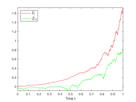
Figure 3: Numerical simulations of Y^\widehat{Y} and Z^1\widehat{Z}_{1}
Refer to caption
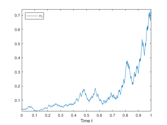
Figure 4: Numerical simulation of vv

It seems that there is no existing literature on numerical methods of equation (5.9), which is a BSDE with filtering. Using Theorem 2.1 in Wang et al. [20] again, we get

{d​φ^=[(A+Υ​Q)​φ^+C1​(1+Υ​N1)−1​η^1]​d​t+η^1​d​W1,φ^T=ζ^,d​ψ^=−{[A+Γ2​B2​R−1+Γ2​C12​Υ​(1+Υ​N1)−1]​ψ^+Γ2​C1​(1+Υ​N1)−1​η^1}​d​t+[(N1−Γ2)​(I+Υ​N1)−1​η^1−C1​(I+Υ​N1)−1​(Γ2​φ^+ψ^)]​d​W1,ψ^0= 0.\left\{\begin{aligned} d\widehat{\varphi}=&\Big[(A+\Upsilon Q)\widehat{\varphi}+C_{1}(1+\Upsilon N_{1})^{-1}\widehat{\eta}_{1}\Big]dt+\widehat{\eta}_{1}dW_{1},\\ \widehat{\varphi}_{T}=&\ \widehat{\zeta},\\ d\widehat{\psi}=&-\Big\{\left[A+\Gamma_{2}B^{2}R^{-1}+\Gamma_{2}C_{1}^{2}\Upsilon(1+\Upsilon N_{1})^{-1}\right]\widehat{\psi}+\Gamma_{2}C_{1}(1+\Upsilon N_{1})^{-1}\widehat{\eta}_{1}\Big\}dt\\ &+\Big[(N_{1}-\Gamma_{2})(I+\Upsilon N_{1})^{-1}\widehat{\eta}_{1}-C_{1}(I+\Upsilon N_{1})^{-1}(\Gamma_{2}\widehat{\varphi}+\widehat{\psi})\Big]dW_{1},\\ \widehat{\psi}_{0}=&\ 0.\end{aligned}\right.

Applying the numerical method introduced in Ma et al. [24], we generate the dynamic simulations of φ^\widehat{\varphi} and η^1\widehat{\eta}_{1}, shown in Fig. 2. For more information about numerical methods for BSDEs, please refer to Peng and Xu [25], Zhao et al. [26] and the references therein. The simulation of ψ^\widehat{\psi} is also shown in Figure 2.

From Theorem 4.1 and Theorem 4.2, we have Y^=Υ​X^+φ^\widehat{Y}=\Upsilon\widehat{X}+\widehat{\varphi}, X^=−Γ2​Y^−ψ^\widehat{X}=-\Gamma_{2}\widehat{Y}-\widehat{\psi} and Z^1=(I+Υ​N1)−1​(η^1−Υ​C1​X^)\widehat{Z}_{1}=(I+\Upsilon N_{1})^{-1}(\widehat{\eta}_{1}-\Upsilon C_{1}\widehat{X}). Then the dynamic simulations of Y^\widehat{Y} and Z^1\widehat{Z}_{1} are similarly generated, shown in Figure 3. Further, from Theorem 4.2, we also generate the dynamic simulation of vv, which is presented in Figure 4.

6 Conclusion

We investigate an LQ control problem of BSDE with partial information, where both the generator of dynamic system and the cost functional contain diffusion terms Z1Z_{1} and Z2Z_{2}. This problem is solved completely and explicitly under some standard conditions. An feedback representation of optimal control and an explicit formula of corresponding optimal cost are given in terms of three Riccati equations, a BSDE with filtering and an SDE with filtering. Moreover, we work out two special scalar-valued control problems to illustrate our theoretical results.

Note that the coefficients in the generator of state equation and the weighting matrices in the cost functional are deterministic. If the coefficients are random, there will be an essential difficulty in solving the case. Since 𝔼⁡[At​Yt|ℱtW1]=At​𝔼​[Yt|ℱtW1]\mathbb{E}[A_{t}Y_{t}|\mathcal{F}_{t}^{W_{1}}]=A_{t}\mathbb{E}[Y_{t}|\mathcal{F}_{t}^{W_{1}}] is no longer true if AA is an {ℱt}t≥0\{\mathcal{F}_{t}\}_{t\geq 0}-adapted stochastic process. We will investigate the stochastic case in future.

References

  • [1] J. M. Bismut, An introductory approach to duality in optimal stochastic control, SIAM Rev. 20 (1978) 62-78.
  • [2] E. Pardoux, S. Peng, Adapted solution of a backward stochastic differential equation, Syst. Control Lett. 14 (1) (1990) 55-61.
  • [3] N. El. Karoui, S. Peng, M. C. Quenez, Backward stochastic differential equations in finance, Math. Finance 7 (1997) 1-71.
  • [4] J. Ma, J. Yong, Forward-backward stochastic differential equations and their applications, Lecture Notes in Math, Springer-Verlag, New York, 1999.
  • [5] M. Kohlmann, X. Zhou, Relationship between backward stochastic differential equations and stochastic controls: a linear-quadratic approach, SIAM J. Control Optim. 38 (5) (2000) 1392-1407.
  • [6] S. Peng, Backward stochastic differential equations and applications to optimal control, Appl. Math. Optim. 27 (2) (1993) 125-144.
  • [7] N. G. Dokuchaev, X. Zhou, Stochastic controls with terminal contingent conditions, J. Math. Anal. Appl. 238 (1999) 143-165.
  • [8] A. E. B. Lim, X. Zhou, Linear-quadratic control of backward stochastic differential equations, SIAM J. Control Optim. 40 (2) (2001) 450-474.
  • [9] X. Li, J. Sun, J. Xiong, Linear quadratic optimal control problems for mean-field backward stochastic differential equations, Appl. Math. Optim. 80 (2019) 223-250.
  • [10] J. Huang, S. Wang, Z. Wu, Backward mean-field Linear-quadratic-gaussian (LQG) games: full and partial information, IEEE Trans. Automat. Control 60 (12) (2016) 3784-3796.
  • [11] K. Du, J. Huang, Z. Wu, Linear quadratic mean-field-game of backward stochastic differential systems, Math. Control Relat. Fields 8 (2018) 653-678.
  • [12] K. Du, Z. Wu, Linear-quadratic stackelberg game for mean-field backward stochastic differential system and application, Math. Probl. Eng. 17 (2019) 1-17.
  • [13] Y. Hu, B. Øksendal, Partial information linear quadratic control for jump diffusions, SIAM J. Control Optim. 47 (4) (2008) 1744-1761.
  • [14] Z. Wu, A maximum principle for partially observed optimal control of forward-backward stochastic control systems, Sci. China Infor. Sci. 53 (11) (2010) 2205-2214.
  • [15] J. Huang, G. Wang, J. Xiong, A maximum principle for partial information backward stochastic control problems with applications, SIAM J. Control Optim. 48 (4) (2009) 2106-2117.
  • [16] G. Wang, Z. Wu, J. Xiong, A linear-quadratic optimal control problem of forward-backward stochastic differential equations with partial information, IEEE Trans. Automat. Control 60 (11) (2015) 2904-2916.
  • [17] G. Wang, H. Xiao, G. Xing, An optimal control problem for mean-field forward-backward stochastic differential equation with noisy observation, Automatica 86 (2017) 104-109.
  • [18] G. Wang, H. Xiao, J. Xiong, A kind of LQ non-zero sum differential game of backward stochastic differential equation with asymmetric information, Automatica 97 (2018) 346-352.
  • [19] J. Yong, X. Zhou, Stochastic Controls: Hamiltonian Systems and HJB Equations, Springer-Verlag, New York, 1999.
  • [20] G. Wang, Z. Wu, J. Xiong, An Introduction to Optimal Control of FBSDE with Incomplete Information, Springer-Verlag, New York, 2018.
  • [21] J. Xiong, An Introduction to Stochastic Filtering Theory, Oxford University Press, London, 2008.
  • [22] R. S. Liptser, A. N. Shiryayev, Statistics of Random Processes, Springer-Verlag, New York, 1977.
  • [23] P. Huang, G. Wang, H. Zhang, A partial information linear-quadratic optimal control problem of backward stochastic differential equation with its applications, Sci. China Infor. Sci. 63 (9) (2020) 1-14.
  • [24] J. Ma, P. Protter, J. S. Martin, S. Torres, Numerical method for backward stochastic differential equations, Ann. Appl. Probab. 12 (2002) 302-316.
  • [25] S. Peng, M. Xu, Numerical algorithms for backward stochastic differential equations with 1-d brownian motion: Convergence and simulations, ESAIM Math. Model. Numer. Anal. 45 (2011) 335-360.
  • [26] W. Zhao, L. Chen, S. Peng, A new kind of accurate numerical method for backward stochastic differential equations, SIAM J. Sci. Comput. 28 (4) (2006) 1563-1581.