Fe VII emission lines in the wavelength range 193–197 ÅJournal: ApJ
Abstract
The identifications of Fe vii emission lines in the wavelength range 193–197 Å are discussed in the light of new measurements of laboratory spectra and atomic data calculations. This region is of importance to studies of solar spectra from the EUV Imaging Spectrometer (EIS) on board the Hinode spacecraft, which has its peak sensitivity at these wavelengths. Ten lines are measured, arising from seven fine structure levels in the configuration. Two lines have not previously been reported and lead to new experimental energies for the levels. Updated experimental energies are obtained for the remaining levels. The new atomic model is used to compute theoretical values for the two density diagnostic ratios 196.21/195.39 and 196.21/196.06, and densities are derived from EIS spectra of coronal loop footpoints.
I Introduction
Fe vii is formed at temperatures 0.2–0.5 MK in the solar atmosphere and produces many emission lines through the extreme ultraviolet (EUV) spectrum from 160 to 300 Å. These offer a number of temperature and density diagnostic ratios (Del Zanna 2009; Young & Landi 2009), and the ion can be used for element abundance diagnostics. For example, the ion is formed at similar temperatures to O v and O vi, which also have lines in the EUV, thus allowing the Fe/O abundance ratio to be measured. This is an important ratio for understanding abundance anomalies in the solar corona (Del Zanna & Mason 2014) and solar wind (Ko et al. 2014). The Fe vii lines also make contributions to the bandpasses of EUV spectroscopic imaging instruments such as the EUV Imaging Telescope (Delaboudinière et al. 1995, EIT;), the Transition Region and Coronal Explorer (Handy et al. 1999, TRACE;), the EUV Imager (Howard et al. 2008, EUVI;), and the Atmospheric Imaging Assembly (Lemen et al. 2012, AIA;). Young & Landi 2009 demonstrated that Fe vii enhanced the 171 and 195 Å channel response functions for TRACE by around 50% at the temperature of formation of the ion, and studies of prominence eruptions have suggested EUV channels can be dominated by ion species formed at 0.2 MK (Ciaravella et al. 2000; Landi et al. 2010).
Fe vii is of particular interest for studies of active region fan loops (Schrijver et al. 1999) and sunspot plumes (Foukal et al. 1974). The lower sections of these structures have a large emission measure at temperatures of 0.2–0.8 MK (Landi & Young 2009), strongly enhancing emission lines in this region. The ion is thus valuable for measuring the temperature gradient in the loops, thus constraining the conductive energy flux.
The EUV Imaging Spectrometer (Culhane et al. 2007, EIS;) on the Hinode spacecraft (Kosugi et al. 2007) has observed the Sun’s EUV spectrum in the bandpasses 170–212 and 246-291 Å for more than 14 years. Landi & Young 2009, Young & Landi 2009 and Del Zanna 2009 presented examples of spectra from fan loops and sunspot plumes, respectively, and compared the Fe vii emission with atomic models formed from the data of Witthoeft & Badnell 2008. However, the two groups of authors came to different conclusions on line identifications in their spectra. In the present work we present analysis of high resolution laboratory spectra, and create a new atomic model using data from Tayal & Zatsarinny 2014 and Li et al. 2018. Our focus is on Fe vii lines in the region 193–197 Å as this contains some of the strongest Fe vii transitions and is also the region where the EIS effective area is highest.
II Atomic data and models
A new atomic model was constructed using the dataset published by Tayal & Zatsarinny 2014, which provided Maxwellian-averaged collision strengths (“upsilons”) and radiative decay rates for 189 levels belonging to the , , () and () configurations. Although Tayal & Zatsarinny 2014 stated their data should be more accurate than earlier works of Zeng et al. 2005 and Witthoeft & Badnell 2008, they also commented that computational limitations meant that configuration interaction effects could not be fully modeled in the scattering calculation. This particularly affects the complex configuration that produces most of the EUV lines.
Only radiative decay rates for allowed transitions were provided by Tayal & Zatsarinny 2014, so forbidden transition rates were taken from Li et al. 2018 and, where necessary, from Witthoeft & Badnell 2008.
Appendix C compares radiative decay rates and upsilons between the different atomic calculations, with agreement found within 25% and 30%, respectively, except for one transition.
Comparisons of calculated and energies with the experimental levels from Ekberg 1981 showed deviations of to cm-1 for Tayal & Zatsarinny 2014, and to cm-1 for Li et al. 2018. Therefore the Li et al. 2018 energies were used for levels with no experimental energies.
Experimental energies are taken from Ekberg 1981, except where these were updated by Young & Landi 2009. Updated energies for five levels are given in the present work, and new energies are provided for two levels (Section IV).
The atomic data were converted to the CHIANTI11 1 https://chiantidatabase.org. database format. In particular, an assessment procedure was applied to the upsilons such that they were scaled and extrapolated using a modification of the Burgess & Tully 1992 method, as described in CHIANTI Technical Report No. 422 2 https://chiantidatabase.org/tech_reports/04_write_scups/chianti_report_04.pdf. The procedure identified a number of transitions for which the allowed transition upsilons did not tend towards the high-temperature limit points. This was likely due to the fact that Tayal & Zatsarinny 2014 used a more elaborate model for the structure calculation compared to the scattering calculation.
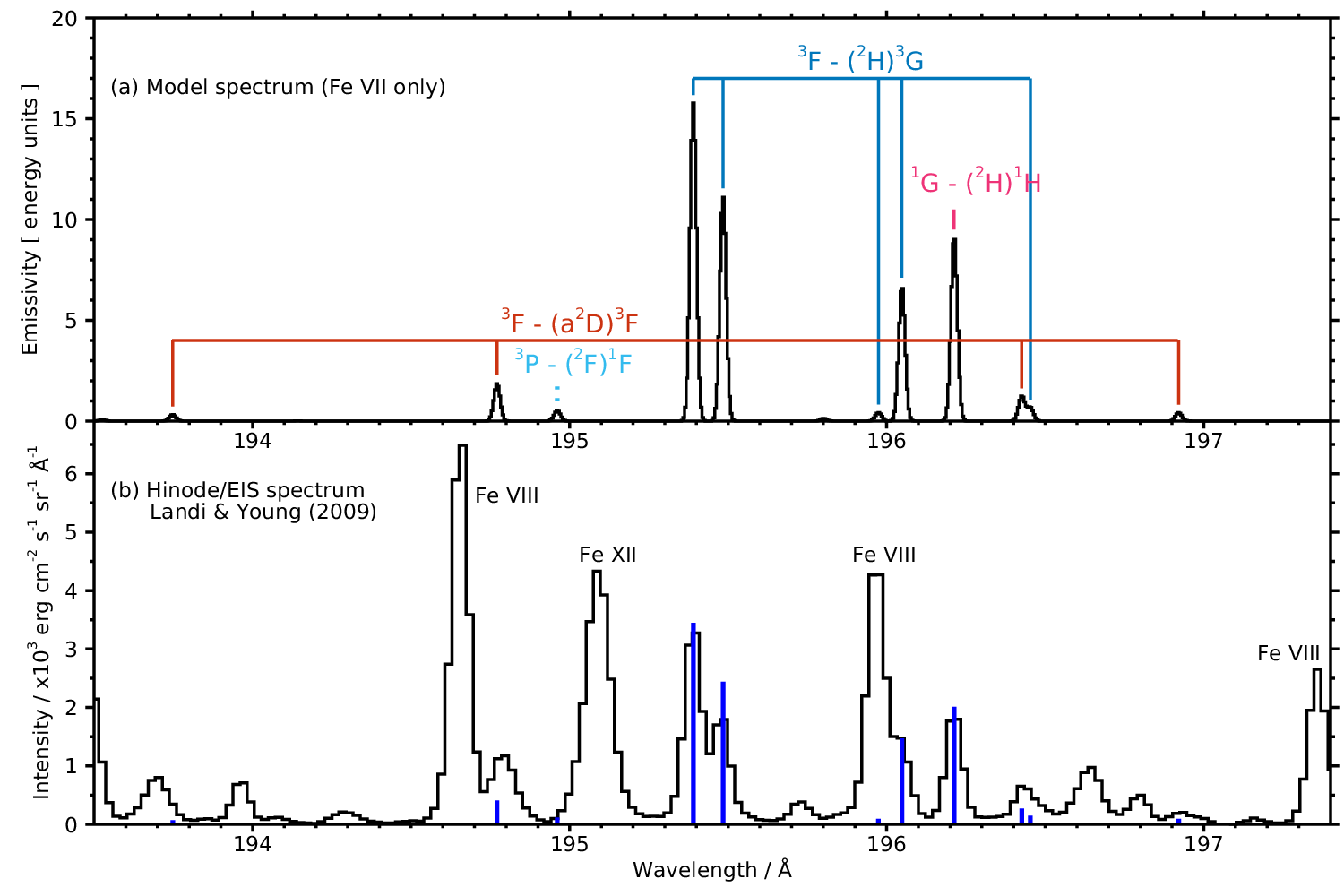
With the data in the CHIANTI format, the CHIANTI IDL software was run to compute emissivities and assess the strengths of the transitions in the 193–197Å region. Although there are uncertainties in the line identifications in this region, it is clear from the atomic models that the only transitions that are relevant belong to four multiplets. In each case the transitions are decays from the configuration to the ground configuration and henceforward we will not refer to the configurations when specifying the transitions. (Thus – is shorthand for – .) The levels are assigned parent terms due to the many duplicate terms in this configuration. The parent term assignments come from the AUTOSTRUCTURE model mentioned in Young & Landi 2009. The multiplets are (in order of importance) – (5 lines), – (1 line), – (3 lines) and – (1 line). Figure 1(a) shows the Fe vii spectrum computed from the current atomic model for a temperature, , of K and electron number density, , of cm-3. The lines belonging to the four multiplets are indicated. The wavelengths of these lines are discussed in the following sections. Figure 1(b) shows the EIS spectrum from Landi & Young 2009 with the model Fe vii intensities from panel (a) over-plotted.
Table 1 gives the emissivities for the eleven transitions considered in this work, computed at and , which are values typical of the solar atmosphere. Additional values are given for , which is the approximate density of the laboratory plasma. Level indices correspond to those given in Table 2 of Tayal & Zatsarinny 2014. The quantity shown is:
| (1) |
where is the energy of the – transition, is the population of the upper level (normalized such that ), and is the radiative decay rate. We note that the contribution function (in the format returned by the CHIANTI IDL routine gofnt) is obtained by multiplying by the ionization fraction and the element abundance, and dividing by .
Comparisons with emissivities constructed from two other atomic models—one of which is that used by Young & Landi 2009—are given in Appendix B. Agreement is found to within 26%, except for one transition that shows differences of up to 43%.
Young & Landi 2009 identified the 196.21/195.39 ratio as a good density diagnostic, with sensitivity over the range to 9.5. From the EIS spectra they derived a density of . However, the 195.39 Å line contains a weak Fe x blend (Young & Landi 2009, noted in) that was not corrected for. Adjusting for this yields a value of . The ratio curve from the new atomic model is shown in Figure 2(a) and compared with the earlier model. It is seen that the ratio is shifted slightly to lower densities, yielding an updated density of . We also show the 196.21/196.05 ratio in Figure 2(b) as the lines are adjacent in the spectrum. The curve is about 10% lower than that from the previous model at high densities, and the measured EIS ratio is close to the high density limit giving a lower limit of . This value is consistent with the density of obtained from the Mg vii 280.72/278.39, which we consider the most accurate diagnostic in this temperature range.
| WavelengthbbUncertainties on the last digit of the present wavelengths are given in parentheses./Å | ccComputed at and densities ./erg cm3 s-1 | |||||||||
|---|---|---|---|---|---|---|---|---|---|---|
| Terms | – | –aaLevel indices of Tayal & Zatsarinny 2014. | Present | Ekberg | Intensity | |||||
| – | 2–3 | 1–106 | 196.049(6) | 196.046 | 7.64 | 6.72 | 6.60 | 4.70 | 4.55 | |
| 3–3 | 2–106 | 196.453(4) | 196.453 | 0.76 | 0.67 | 0.66 | 0.47 | 0.67 | ||
| 3–4 | 2–108 | 195.480(4) | 13.51 | 11.15 | 10.83 | 7.15 | 7.28 | |||
| 4–4 | 3–108 | 195.971(4) | 0.51 | 0.42 | 0.41 | 0.27 | 2.58ddBlended with Fe viii. | |||
| 4–5 | 3–109 | 195.392(4) | 195.391 | 17.23 | 15.77 | 15.47 | 10.00 | 14.25 | ||
| – | 2–2 | 1–110 | 193.744(4) | 0.31 | 0.33 | 0.34 | 0.19 | 0.18 | ||
| 3–3 | 1–107 | 194.770(4) | 2.01 | 1.87 | 1.86 | 1.59 | 1.06 | |||
| 3–4 | 2–105 | 196.426(6) | 196.423 | 1.27 | 1.23 | 1.27 | 0.88 | 2.61 | ||
| 4–4 | 3–105 | 196.920(6) | 196.917 | 0.43 | 0.42 | 0.44 | 0.30 | 0.36 | ||
| – | 4–5 | 8–114 | 196.216(5) | 6.68 | 9.20 | 9.56 | 6.46 | 6.46eeLaboratory intensities are normalized to this line. | ||
| – | 2–3 | 7–111 | 194.961ffTheoretical wavelength from Li et al. 2018. | 0.46 | 0.53 | 0.56 | 0.31 | |||

III Laboratory spectra
Spectra in the wavelength range 90–350 Å were obtained from a high resolution grazing incidence spectrograph with a 3 m (3600 lines/mm) grating. Previous spectra used for the analysis of Fe viii (Ramonas & Ryabtsev 1980) were recorded on photographic plates, whereas Fuji Imaging Plates were used for the new spectra (Ryabtsev 2017). The FWHM values of the lines in the 200 Å region are 0.017 Å and 0.024 Å for the photoplates and imaging plates, respectively, corresponding to spectral resolutions () of 12 000 and 8000. (These compare with a resolution of 3000 for the Hinode/EIS instrument at 195 Å.) Although having worse resolution, the imaging plate spectra possess a high linearity of the line intensities. The wavelengths were measured from the photoplate spectra whereas the line intensity data were obtained from the imaging plate spectra. The estimated uncertainty of the wavelengths is from 0.004 Å to 0.006 Å. The intensities are given on a relative scale without taking into account possible wavelength variation of the setup sensitivity. The spectra were excited in a vacuum spark run from a capacitor with or 150 F, charged from 1 to 5 kV. The observation of the changes of the line intensities with a variation of the discharge conditions served for a separation of the lines belonging to different iron ions. Further experimental details can be found in the earlier references.
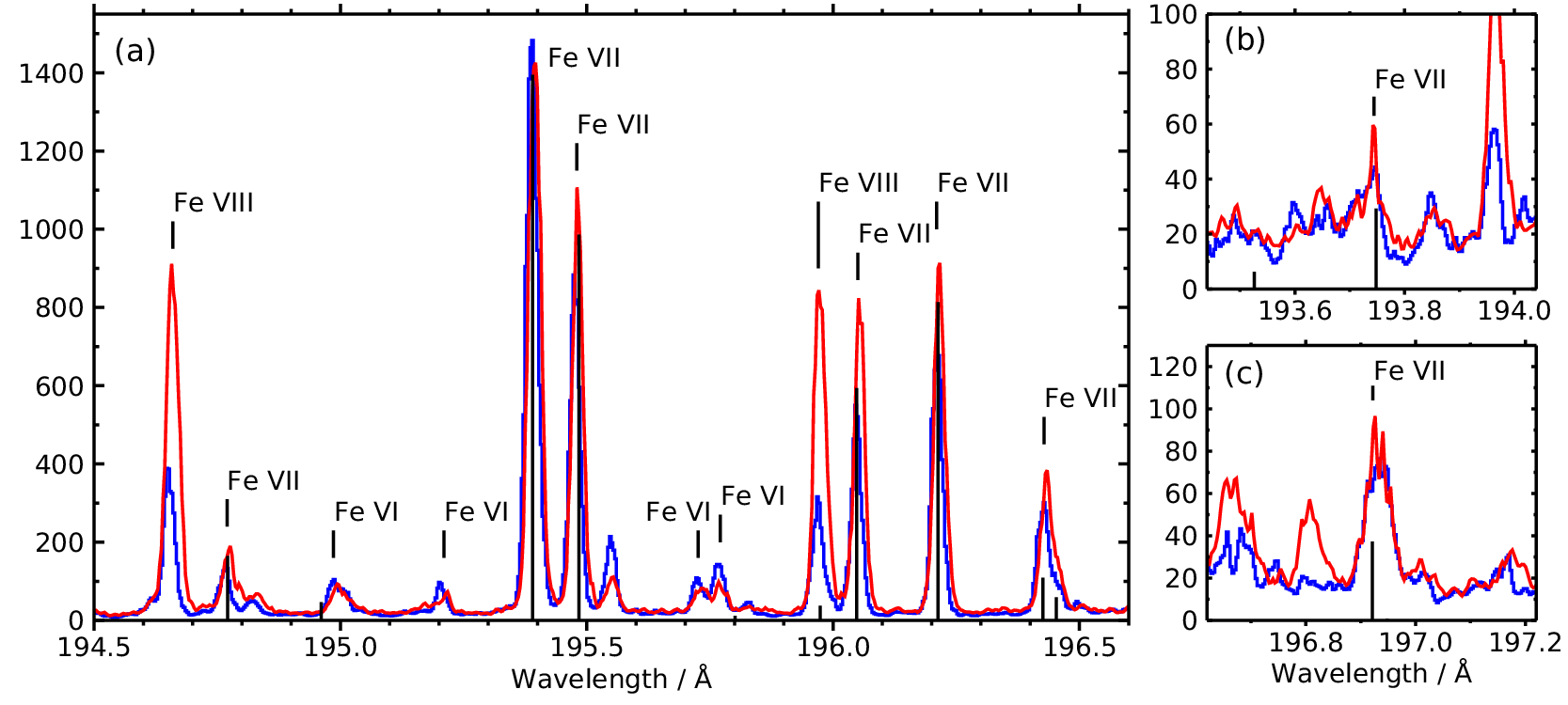
Figure 3 shows spectra from the photoplate data, which have a higher spectral resolution. Appendix A discusses the imaging plate spectra, which were used for intensity measurements due to the high signal linearity. Three sections of the iron spark spectra are shown in Figure 4: the strong lines between 194.5 and 196.6 Å (a), and the two weak lines at 193.7 and 196.9 Å (b and c). In each panel the “cold” and “hot” spectra are shown as blue and red lines, respectively. Lines due to Fe viii are about twice as strong in the hot spectra, and the strong lines at 194.66 Å and 195.97 Å are clearly seen. Fe vi identifications are from Azarov et al. 1996 and the lines are generally weaker in the hot spectrum. Fe vii lines have comparable intensities in the two spectra and, by comparing with the model spectrum shown in Figure 1, one can see there is a good match in terms of relative intensities. There are a number of unidentified lines, with the most significant being that at 195.53 Å, and they are likely due to Fe v or Fe vi. The strong Fe ix 197.86 line is not present, implying an absence of species hotter than Fe viii.
The wavelengths measured from the laboratory spectrum are given in the third column of Table 1, alongside the measured values of Ekberg 1981. The final column of Table 1 gives the line intensities measured from the imaging plate spectrum, with the values normalized to the theoretical emissivity of the line at 196.216 Å at . We note that the intensities are not corrected for the spectrograph efficiency as a function of wavelength, but this effect should be small given the narrow spectral range considered here. The line at 195.971 Å is blended with a Fe viii transition that is significantly stronger, and the line at 196.922 Å is blended with Fe vi, although in this case the Fe vii line is dominant.

| Terms | – | E81 | YL09 | DZ09 | Present | Li18 | |
|---|---|---|---|---|---|---|---|
| – | 2–3 | 196.046 | 196.045 | 197.358 | 196.049 | 195.737 | |
| 3–3 | 196.453 | 196.450 | 197.769 | 196.453 | 196.229 | ||
| 3–4 | 196.423 | 195.480 | 196.210 | 195.480 | 194.691 | ||
| 4–4 | 196.917 | 195.970 | 196.704 | 195.971 | 195.177 | ||
| 4–5 | 195.391 | 195.388 | 196.046 | 195.392 | 194.450 | ||
| – | 2–2 | – | 193.788aaEstimated wavelengths (see main text). | – | 193.744 | 193.498 | |
| 2–3 | – | 194.728aaEstimated wavelengths (see main text). | – | 194.770 | 194.453 | ||
| 3–4 | – | 196.423 | – | 196.426 | 196.150 | ||
| 4–4 | – | 196.918 | – | 196.920 | 196.643 | ||
| – | 4–5 | – | 196.212 | 196.209 | 196.216 | 195.073 |
IV Line identifications
Table 2 summarizes the experimental wavelengths in the 193–197 Å range that were reported by Ekberg 1981, Young & Landi 2009 and Del Zanna 2009. Also shown are the wavelengths obtained from the theoretical energy values of Li et al. 2018. Table 3 compares the experimental energies with the theoretical energies of Witthoeft & Badnell 2008, Tayal & Zatsarinny 2014 and Li et al. 2018. For levels within a multiplet, the lowest energy level is listed with the energy splitting relative to this level given for the remaining levels.
| Term | J | Index | WB08 | TZ14 | Li18 | E81 | YL09 | DZ09 | Present |
|---|---|---|---|---|---|---|---|---|---|
| 3 | 106 | 524 582 | 527 900 | 511 940 | 510 086 | 510 086 | 506 693 | 510 080 | |
| 4 | 108 | +3082 | +2700 | +2747 | +72 | +2527 | +4016 | +2522 | |
| 5 | 109 | +5313 | +4500 | +4663 | +4047 | +4047 | +5722 | +4049 | |
| 4 | 105 | 523 308 | 527 300 | 510 866 | 510 158 | 510 149 | |||
| 3 | 107 | +3379 | +3200 | +3398 | +3379aaEstimated energies with an accuracy of 200 cm-1. | +3274 | |||
| 2 | 110 | +5871 | +5400 | +5936 | +5871aaEstimated energies with an accuracy of 200 cm-1. | +5986 | |||
| 3 | 111 | 547 153 | 546 400 | 534 202 | |||||
| 5 | 114 | 556 628 | 552 200 | 541 557 | 538 566 | 538 588 | 538 578 |
Ekberg 1981 was the first to perform a detailed study of the Fe vii EUV spectrum using laboratory spectra, and this was the starting point of the Young & Landi 2009 analysis. A key discrepancy was found for the level, which Ekberg 1981 identified with emission lines at 196.42 and 196.92 Å (Table 2) leading to an energy only 72 cm-1 greater than that of (Table 3). The three theoretical works consistently yield a much larger separation of 2700–3100 cm-1. This led to Young & Landi 2009 identifying the level with the strong line at 195.48 Å, which gives better agreement with the theoretical energy splittings. We note here an error in Table 3 of Young & Landi 2009 whereby the energy of 512 601 cm-1 for should have been given as cm-1, which is derived from the 195.48 Å line measured in the EIS spectrum. It is the latter value that is given in Table 3. The laboratory spectra presented here clearly demonstrate that the 195.48 Å line is due to Fe vii. A comparison of the model emissivities with the laboratory intensities (Table 1) also clearly shows that the strength of the 195.48 Å line is much more consistent with the level than the weak line at 196.42 Å.
With the lines measured by Ekberg 1981 at 196.42 and 196.92 Å no longer associated with , Young & Landi 2009 identified them with . Table 1 shows that the model emissivity for the 196.92 Å line is in good agreement with the laboratory intensity, but the 196.42 Å measured intensity is much stronger than expected. However, no other level identification is suitable and so we believe these identifications are correct. Young & Landi 2009 did not identify the 196.92 Å line in their spectrum, but they did measure a line at 196.964 Å. Correcting this wavelength for the plasma Doppler shift gives 196.937 Å. The intensity ratio relative to the 196.42 Å line is 0.77, significantly larger than the theoretical ratio of 0.34 (Table 1). Thus the solar line at 196.94 Å appears to be blended.
Young & Landi 2009 adjusted the theoretical energies of the levels based on the theoretical splittings relative to leading to improved estimates of the wavelengths of lines from these levels. It was not possible to identify these transitions in the EIS spectra, but they are apparent in the laboratory spectra close to the predicted wavelengths and are shown in Figure 3. The emissivity comparison is good for these lines (Table 1), giving confidence in the identifications. We therefore give new experimental energies for these two levels in Table 3, which we estimate to be accurate to 9 cm-1 (Table 4).
Ekberg 1981 was not able to identify the strong – transition, perhaps because no other transitions from the level could be found in the spectrum. Young & Landi 2009 identified it with the 196.21 Å line as it could be clearly identified with Fe vii in the EIS spectra and the intensity was consistent with nearby Fe vii lines. This is confirmed with the laboratory spectra here.
The line at 196.45 Å was identified by Ekberg 1981, but was blended in the EIS spectra. Figure 3 clearly shows this line as a “shoulder” on the long-wavelength side of the stronger 196.42 Å line and the intensity is in reasonable agreement with the model (Table 1).
Finally we consider the – transition, which is estimated at 194.96 Å using the Li et al. 2018 theoretical energy. By comparison with the and levels that are close to and have experimental energies, we can estimate that the Li et al. 2018 energy over-estimates the true energy by between 2300 and 3000 cm-1. This would place the – transition between 195.84 and 196.11 Å, close to the strong Fe viii and Fe vii lines in this range (Figure 3). As no candidate can be seen, then it is possible the line is blended with one of these lines.
V Discussion
The previous section showed that the Fe vii line identifications in the 193–197 Å range are now complete except for the weak – transition. In this section we discuss additional issues related to these lines.
Del Zanna 2009 presented an analysis of the EIS Fe vii spectrum using an atomic model constructed from the Witthoeft & Badnell 2008 collision strengths and the radiative decay rates from his own structure calculation. He identified the observed 196.21 Å line with the – transition, consistent with Young & Landi 2009. A key difference with Young & Landi 2009, however, is that he modified the line identifications of all of the levels, giving the wavelengths listed in Table 2. In particular, the strong – () transitions were matched to the observed lines at 197.36, 196.21 and 196.05 Å. The 197.36 Å line is blended with a much stronger Fe viii line and the 196.21 Å line is a self-blend with the – transition. These identifications were motivated by the fact that the observed line at 195.39 Å seemed to be too strong in the EIS spectrum, and that the image formed in this line was more consistent with Fe viii. By switching the identification to the weaker 196.05 Å line these problems could be solved.
The laboratory spectrum presented here clearly demonstrates that the 195.39 Å line is due to Fe vii. The emissivity comparison does show that the measured line is stronger than expected compared to other lines by around 30%. This may indicate a Fe vi blend (see Appendix A). The fact that the solar image formed from the EIS line appears to be hotter than Fe vii was explained by Young & Landi 2009 as due to a blend with a Fe x line.
A further problem with the Del Zanna 2009 identifications is that they require fortuitous blends with strong lines. Both lines are very narrow in the solar spectra (Landi & Young 2009), and thus the two Del Zanna 2009 identifications require very precise wavelength matches, which seems an unlikely coincidence. The Del Zanna 2009 level splittings are in worse agreement with theory compared to our new measurements (Table 3), and the 196.45 Å line is inconsistent with the upper level being as the – transition is forbidden.
Although we are confident in the line identifications given in Table 2, we highlight that the lines at 195.39 Å and 196.42 Å are significantly stronger than the other lines. Almost a factor three in the latter case. Blending is a possibility but we also note the conclusion of Tayal & Zatsarinny 2014 that their scattering calculation could not include all of the configuration interaction terms necessary to fully model the configuration. We illustrate why this is important in Table 4, which gives the mixing coefficients for the levels considered here, computed with the Cowan atomic code by one of us (A. Ryabtsev). (The listed theoretical energies come from this calculation.) All of the and levels are highly mixed and so it is important that the scattering calculation accurately takes into account this mixing. We also highlight that the “” (Young & Landi 2009, the parent term being assigned by) level actually has a dominant contribution from in this calculation, illustrating how mixing can change with different calculations.
| Energy/cm-1 | |||||
|---|---|---|---|---|---|
| Term | ExperimentalaaThe number in parentheses gives the uncertainty on the last digit. | Theoretical | Difference | Percentage contributionsbbAll terms belong to the configuration; only contributions of % are shown. | |
| () | 3 | 510080(6) | 509469 | +611 | 44% + 22% + 17% |
| 4 | 512602(9) | 512098 | +504 | 48% + 18% + 18% | |
| 5 | 514129(8) | 514066 | 54% + 22% + 12% | ||
| () | 4 | 510149(11) | 509143 | +1006 | 37% + 21% + 17% |
| 3 | 513423(9) | 512035 | +1388 | 36% + 19% + 18% | |
| 2 | 516135(9) | 514542 | +1593 | 43% + 21% + 17% | |
| () | 3 | 531117 | 34% + 23% + 21% | ||
| () | 5 | 538578(11) | 538227 | +351 | 92% |
VI Summary
A new atomic model constructed from the atomic data of Tayal & Zatsarinny 2014 has been presented along with high-resolution laboratory spectra of Fe vii lines. The spectra are important for confirming Fe vii line identifications in the range 193–197 Å, which is relevant to the study of spectra from the Hinode/EIS instrument. In particular the strong lines at 195.39 and 195.48 Å are clearly seen to be due to Fe vii. Two new line identifications have been made, leading to new experimental energies for the levels. The new model was recently released to the community through version 10 of the CHIANTI database (Del Zanna et al. 2020).
The intensities of the lines at 195.39 Å and 196.42 Å are stronger in the laboratory spectrum compared to the atomic model. This may be due to blending and/or uncertainties in the atomic data.
A detailed study of the entire Fe vii laboratory spectrum will follow, and will be used to address some of the other issues highlighted by Del Zanna 2009 and Young & Landi 2009.
References
- Azarov et al. (1996) Azarov, V. I., Podobedova, L. I., & Ryabtsev, A. N. 1996, Phys. Scr, 53, 398, doi: 10.1088/0031-8949/53/4/003
- Burgess & Tully (1992) Burgess, A., & Tully, J. A. 1992, A&A, 254, 436
- Ciaravella et al. (2000) Ciaravella, A., Raymond, J. C., Thompson, B. J., et al. 2000, ApJ, 529, 575, doi: 10.1086/308260
- Culhane et al. (2007) Culhane, J. L., Harra, L. K., James, A. M., et al. 2007, Sol. Phys., 243, 19, doi: 10.1007/s01007-007-0293-1
- Del Zanna (2009) Del Zanna, G. 2009, A&A, 508, 501, doi: 10.1051/0004-6361/200913082
- Del Zanna et al. (2020) Del Zanna, G., Dere, K. P., Young, P. R., & Landi, E. 2020, arXiv e-prints, arXiv:2011.05211. https://arxiv.org/abs/2011.05211
- Del Zanna & Mason (2014) Del Zanna, G., & Mason, H. E. 2014, A&A, 565, A14, doi: 10.1051/0004-6361/201423471
- Delaboudinière et al. (1995) Delaboudinière, J. P., Artzner, G. E., Brunaud, J., et al. 1995, Sol. Phys., 162, 291, doi: 10.1007/BF00733432
- Ekberg (1981) Ekberg, J. O. 1981, Phys. Scr, 23, 7, doi: 10.1088/0031-8949/23/1/002
- Foukal et al. (1974) Foukal, P. V., Noyes, R. W., Reeves, E. M., et al. 1974, ApJ, 193, L143, doi: 10.1086/181651
- Handy et al. (1999) Handy, B. N., Acton, L. W., Kankelborg, C. C., et al. 1999, Sol. Phys., 187, 229, doi: 10.1023/A:1005166902804
- Howard et al. (2008) Howard, R. A., Moses, J. D., Vourlidas, A., et al. 2008, Space Sci. Rev., 136, 67, doi: 10.1007/s11214-008-9341-4
- Ko et al. (2014) Ko, Y.-K., Muglach, K., Wang, Y.-M., Young, P. R., & Lepri, S. T. 2014, ApJ, 787, 121, doi: 10.1088/0004-637X/787/2/121
- Kosugi et al. (2007) Kosugi, T., Matsuzaki, K., Sakao, T., et al. 2007, Sol. Phys., 243, 3, doi: 10.1007/s11207-007-9014-6
- Landi et al. (2010) Landi, E., Raymond, J. C., Miralles, M. P., & Hara, H. 2010, ApJ, 711, 75, doi: 10.1088/0004-637X/711/1/75
- Landi & Young (2009) Landi, E., & Young, P. R. 2009, ApJ, 706, 1, doi: 10.1088/0004-637X/706/1/1
- Lemen et al. (2012) Lemen, J. R., Title, A. M., Akin, D. J., et al. 2012, Sol. Phys., 275, 17, doi: 10.1007/s11207-011-9776-8
- Li et al. (2018) Li, Y., Xu, X., Li, B., Jönsson, P., & Chen, X. 2018, MNRAS, 479, 1260, doi: 10.1093/mnras/sty1534
- Ramonas & Ryabtsev (1980) Ramonas, A. A., & Ryabtsev, A. N. 1980, Optics and Spectroscopy, 48, 348
- Ryabtsev (2017) Ryabtsev, A. N. 2017, in European Physical Journal Web of Conferences, Vol. 132, European Physical Journal Web of Conferences, 03043, doi: 10.1051/epjconf/201713203043
- Schrijver et al. (1999) Schrijver, C. J., Title, A. M., Berger, T. E., et al. 1999, Sol. Phys., 187, 261, doi: 10.1023/A:1005194519642
- Tayal & Zatsarinny (2014) Tayal, S. S., & Zatsarinny, O. 2014, ApJ, 788, 24, doi: 10.1088/0004-637X/788/1/24
- Witthoeft & Badnell (2008) Witthoeft, M. C., & Badnell, N. R. 2008, A&A, 481, 543, doi: 10.1051/0004-6361:20079073
- Young & Landi (2009) Young, P. R., & Landi, E. 2009, ApJ, 707, 173, doi: 10.1088/0004-637X/707/1/173
- Zeng et al. (2005) Zeng, J., Liang, G. Y., Zhao, G., & Shi, J. R. 2005, MNRAS, 357, 440, doi: 10.1111/j.1365-2966.2004.08561.x
Appendix A Laboratory spectra obtained with imaging plates
The spectra obtained with the Fuji Imaging Plates are shown in Figure 4. As with the photoplate spectra shown in Figure 3, the blue and red lines correspond to “cold” and “hot” spectra. The latter displays stronger lines from Fe viii, while the former have stronger lines from Fe vi. The spectral resolution is a little worse in these spectra, as can been seen by comparing the feature at 196.4 Å with Figure 3, where two components are clearly seen. The imaging plate spectra have an almost linear intensity scaling and so were used to derive the intensities given in Table 1. The Fe vii lines are generally stronger in the red spectrum, although the strongest line at 195.39 Å is a little weaker in the red spectrum. This may indicate a partial blend with a Fe vi line, although Fe vii dominates. This effect was not seen in the photoplate spectra (Figure 3).
Appendix B Emissivity comparison
The atomic model used in this paper was largely based on the Tayal & Zatsarinny 2014 atomic data. In Table 5 we compare the emissivities from this model with those from two other models that are indicated with “WB08” and “Li08”. The former is the same model as used by Young & Landi 2009, while the latter is the WB08 model but with the radiative decay rates replaced by those of Li et al. 2018, where available. Note that Witthoeft & Badnell 2008 and Tayal & Zatsarinny 2014 provided data for the same 189 fine structure levels, but Li et al. 2018 gave decay rates for a reduced set of 134 levels.
The WB08 and TZ14 emissivities show good agreement, with the largest difference for the 194.77 Å line, which is up to 43% larger in the WB08 model. The median difference between the two models is 7%. The effect of using the Li et al. 2018 decay rates for the WB08 model is relatively small, with a maximum difference of 19% for the weak line at 194.96 Å. The median difference for all transitions is 2.4%.
| cm-3 | cm-3 | cm-3 | |||||||||
|---|---|---|---|---|---|---|---|---|---|---|---|
| /Å | WB08 | Li18 | TZ14 | WB08 | Li18 | TZ14 | WB08 | Li18 | TZ14 | ||
| 196.05 | 6.67 | 6.49 | 7.65 | 5.64 | 5.73 | 6.72 | 5.49 | 5.60 | 6.60 | ||
| 196.46 | 0.71 | 0.63 | 0.76 | 0.60 | 0.55 | 0.67 | 0.58 | 0.54 | 0.66 | ||
| 195.48 | 13.19 | 12.88 | 13.51 | 10.89 | 10.89 | 11.15 | 10.55 | 10.60 | 10.83 | ||
| 195.97 | 0.49 | 0.47 | 0.51 | 0.40 | 0.39 | 0.42 | 0.39 | 0.38 | 0.41 | ||
| 195.39 | 17.06 | 16.87 | 17.22 | 15.86 | 15.65 | 15.77 | 15.55 | 15.36 | 15.46 | ||
| 193.75 | 0.38 | 0.37 | 0.31 | 0.41 | 0.41 | 0.33 | 0.43 | 0.43 | 0.34 | ||
| 194.77 | 2.87 | 2.76 | 2.01 | 2.56 | 2.55 | 1.87 | 2.54 | 2.54 | 1.86 | ||
| 196.42 | 1.00 | 1.06 | 1.27 | 1.09 | 1.17 | 1.23 | 1.20 | 1.29 | 1.27 | ||
| 196.92 | 0.44 | 0.38 | 0.43 | 0.48 | 0.41 | 0.42 | 0.53 | 0.46 | 0.44 | ||
| 196.21 | 6.18 | 6.31 | 6.67 | 8.64 | 8.65 | 9.20 | 9.02 | 8.99 | 9.56 | ||
| 194.96 | 0.45 | 0.37 | 0.46 | 0.54 | 0.44 | 0.53 | 0.57 | 0.46 | 0.56 | ||
Appendix C Comparison of decay rates and upsilons
Appendix B compared emissivities computed from three atomic models. Here we compare radiative decay rates and upsilons for the strongest transitions. Tables 6 gives decay rates from WB08, TZ14 and Li18, and also those from Del Zanna 2009. For the decay rates the agreement is generally very good. The TZ14 rates are larger than the other two calculations for all but two of the transitions. The biggest discrepancy is for the – transition, which is 92% higher than WB08 and 65% higher than Li18. The WB08 and Li18 data-sets agree very well for the – transitions, with decay rates within 6%. For the other two multiplets agreement is within 25%. A problem can be seen with the DZ09 rates whereby the – 3–4 transition is weaker than the 2–3 transition. This may be a tabulation error.
| Term | – | WB08 | DZ09 | TZ14 | Li18 |
|---|---|---|---|---|---|
| – | 2–3 | 2.86(+10) | 3.30(+10) | 3.82(+10) | 3.02(+10) |
| 3–3 | 3.05(+9) | 3.81(+9) | 2.91(+9) | ||
| 3–4 | 4.27(+10) | 2.40(+10) | 4.90(+10) | 4.14(+10) | |
| 4–4 | 1.59(+9) | 1.86(+9) | 1.50(+9) | ||
| 4–5 | 5.03(+10) | 4.60(+10) | 5.78(+10) | 4.93(+10) | |
| – | 2–2 | 1.12(+9) | 1.19(+9) | 1.07(+9) | |
| 2–3 | 1.12(+10) | 9.00(+9) | 8.44(+9) | ||
| 3–4 | 1.76(+9) | 3.38(+9) | 2.05(+9) | ||
| 4–4 | 7.77(+8) | 1.16(+9) | 7.28(+8) | ||
| – | 4–5 | 3.80(+10) | 3.50(+10) | 4.04(+10) | 4.12(+10) |
| – | 2–3 | 1.31(+9) | 1.58(+9) | 1.32(+9) |
For each of the eight emitting levels considered in this work we compare the WB08 and TZ14 upsilons for the dominant transitions to these levels in Table 7. As expected, the differences mirror those seen in the decay rate calculation. The largest difference is for –, for which the TZ14 upsilon is 72% higher than the WB08 upsilon. The upsilons for other transitions are within 30%.
| Upper | Lower | WB08 | TZ14 |
|---|---|---|---|
| 3.49 | 3.77 | ||
| 2.32 | 2.54 | ||
| 1.22 | 1.58 | ||
| 0.110 | 0.189 | ||
| 0.070 | 0.078 | ||
| 0.484 | 0.366 | ||
| 0.035 | 0.035 | ||
| 2.85 | 3.02 | ||
| 0.077 | 0.092 |