Coupled Maxwell and Time-Dependent Orbital Free Density Functional Calculations
Abstract
Coupled Maxwell and time-dependent orbital-free calculations are implemented and tested to describe the interaction of electromagnetic waves and matter. The currents and induced fields predicted by the orbital-free calculations are compared to time-dependent density functional calculations and very good agreement is found for various systems including jellium sheets, jellium spheres, atomistic sheets and icosahedron clusters.
I Introduction
Ground state density functional theory (DFT) Hohenberg and Kohn 1964 Kohn-Sham (KS) Kohn and Sham 1965 calculations are very successful in condensed matter physics, because they provide a reasonably accurate description of material properties in a computationally manageable way. Mostly these DFT calculations are based on KS orbitals and albeit some approaches scale linearly with the number of orbitals Goedecker 1999; Bowler and Miyazaki 2012 for certain systems, in general KS orbital based DFT has cubic scaling with respect to the system size. Orbital-free (OF) DFT Wang and Carter 2002; Wesolowski and Wang 2013; Karasiev et al. 2014; Witt et al. 2018 became an attractive alternative because its main variable is the electron density and it computationally scales linearly with system size. OF-DFT has shown considerable success in million-atom material simulations of metals, Witt et al. 2018; Shao et al. 2018; Hung and Carter 2009, warm dense matter White et al. 2013; Ding et al. 2018, quantum dots Mi and Pavanello 2019; Shao et al. 2020; Ho et al. 2007; Aguado 2001; Aguado et al. 2001. Computer codes for efficient implementation of OF-DFT have also been developed Chen et al. 2015; Shao et al.; Shao et al. 2018; Golub and Manzhos 2020.
OF-DFT directly calculates the ground-state electron density minimizing the energy functional without using KS orbitals. The minimization leads to a single Schrödinger-like equation. This equation contains a potential, that is derived from the kinetic energy (KE) functional Holas and March 1991; Levämäki et al. 2014 to enforce the antisymmetry requirement of the many-electron wave function.
Time-dependent problems, e.g. calculation of electronic stopping power White et al. 2018; Ding et al. 2018, spectra of clusters Shao et al., plasmonics Xiang et al. 2016; Xiang et al. 2020; Xiang et al. 2014 have been also studied with the ”time-dependent” OF (TD-OF) approach. In this case a single time-dependent Schrödinger equation has to be solved with the additional difficulty that the KE potential is time-dependent Neuhauser et al. 2011.
The main difficulty of the OF calculations is finding the appropriate approximations for the kinetic energy functional. The simplest approximations use local or semilocal expressions, where the energy density depends only on the density and its derivatives at one spatial point Levy and Ou-Yang 1988; Karasiev et al. 2012; Luo et al. 2018; Constantin et al. 2019; Constantin et al. 2018; Lehtomäki and Lopez-Acevedo 2019. However, the local and semilocal KE functionals do not have the correct linear response properties. To correct this, nonlocal (or two-point) KE functionals were developed invoking the linear response of the noninteracting homogeneous electron gas Smargiassi and Madden 1994; Wang and Teter 1992; Perrot 1994. These nonlocal KE functionals work well for a nearly free electron gas and were developed further for more complicated cases Chacón et al. 1985; Wang et al. 1998; Wang et al. 1999; Xia and Carter 2012. These functionals are computationally expensive because they depend explicitly on density at two spatially separated points. More recently, efficient alternatives based on a line integral representation of the KE functional have been proposed and tested Mi et al. 2018; Xu et al. 2019; Mi and Pavanello 2019. While nonlocal functionals are considered to be superior, semilocal functionals are faster and new semilocal functionals have been developed that show very good accuracy Constantin et al. 2018; Lehtomäki and Lopez-Acevedo 2019. Recent advances in machine learning techniques were also put to work in quest of better KE functionals Golub and Manzhos 2020; Seino et al. 2019; Meyer et al. 2020; Fujinami et al. 2020; Manzhos and Golub 2020.
The development of dynamic KE functionals for time-dependent problems is less advanced than the static ones. In Ref. Neuhauser et al. 2011, a dynamic KE potential is proposed that is time propagated and forces the system to closely fit the susceptibility of the noninteracting homegeneous electron gas (Lindhard function) Lindhard. In Ref. White et al. 2018 a local current density dynamic KE potential is derived by perturbation theory. This approach is computationally more efficient because it does not require the time propagation of the KE potential. Both approaches seem to reproduce the frequency dependent Lindhard function nicely.
In this work we use the TD-OF approach coupled with the Maxwell equations to describe the interaction of electromagnetic waves and matter. In a previous paper Covington et al. 2019 we developed a method to solve the coupled Maxwell TD-KS equations. In this coupled frame, the densities and current are calculated in a quantum mechanical framework in the presence of a time-dependent vector potential and then the Maxwell equations are solved with the calculated time-dependent microscopic currents and densities to obtain the new vector potential. In order for the coupling of the quantum and Maxwell dynamics to be significant one needs large systems with many electrons. One can use Time Dependent Density Functional Theory (TDDFT) Runge and Gross 1984 (as we did in Ref. Covington et al. 2019), but that limits the application to relatively small systems. The OF approach allows the simulation of much larger systems (on the scale of millions of atoms Witt et al. 2018; Shao et al. 2018; Hung and Carter 2009; White et al. 2013; Ding et al. 2018; Mi and Pavanello 2019; Shao et al. 2020). The OF approach may allow for electrodynamic simulations to be performed for systems of relevant size with a quantum description of the electrons.
The goal of this paper is to implement coupled Maxwell TD-OF calculations and test them against TDDFT results. We will solve the TD-OF and TDDFT equations using a real–space grid and real–time propagation Varga and Driscoll 2011. The Maxwell-equations are solved using the Riemann-Silberstein formalism Jestädt et al. 2019; Covington et al. 2019. To make the TD-OF and TDDFT calculations comparable we add a constraining potential to the TD-OF Hamiltonian. This potential ensures that the initial ground state densities are the same in the OF and DFT calculations.
II Formalism
II.1 Time-dependent Kohn-Sham equations
The time-dependent Kohn-Sham (TD-KS) equation for the the electron orbital is
| (1) |
where
| (2) |
The Kohn-Sham potential,
| (3) |
is a sum of the external potential, the Hartree and the exchange correlation terms. The vector potential, describes the electromagnetic fields. The TD-KS equations can be solved by time propagation and one can calculate the electron density and current at any time as
| (4) |
| (5) |
where is the number of electrons in the system and each orbital is occupied by two electrons. This current is input into the Maxwell equations, which will then propagate a vector potential .
II.2 Time-dependent Orbital Free equations
The time-dependent orbital free (TD-OF) equation is
| (6) |
where
| (7) |
The orbital free potential is defined as
| (8) |
where is the Thomas-Fermi kinetic energy functional, is the von Weizsäcker potential and is a constraining potential that we will define later. is a numerical coefficient of the Weizsäcker term. Normally the Weizsäcker term comes with an ”” multiplier (with values =1 to 1/9). Here appears because the one has to compensate the appropriate part in the kinetic energy in Eq. (6). In this case the electron density and current at any time is
| (9) |
| (10) |
II.3 Constrained minimization
To compare TDDFT and OF one ideally would use the same ground state density, but and produce different densities, and , respectively. In Ref. Kidd et al. 2018 we have presented a constrained density functional approach. This method can be used to generate a constraining potential that forces the charge density to be equal to a prescribed density. In the present case we will use the constraint
| (11) |
where is the density of the ground state DFT calculation.
The following iterative procedure can be used to calculate the constraining potential:
| (12) |
where controls the convergence,
| (13) |
is the energy expectation value, and is the density operator such that
| (14) |
Given a desired initial density distribution one looks for the potential
| (15) |
which constrains the density according to Eq. (11).
The constrained minimization allows us to construct an orbital free Hamiltonian, , that produces the same self consistent potential and density as the TDDFT calculation. In this way the TDDFT and the OF calculation can be directly compared. Since the constrained ground state density is the same, by setting
| (16) |
the contributions to the energy from the potentials are the same:
| (17) |
The kinetic energy parts in OF
| (18) |
and in TDDFT
| (19) |
are different, although in numerical calculations the difference is small. The constraining potential forces to match the ground state OF density to the DFT density, and then applied the OF Hamiltonian. The constraining potential is kept fixed during the time evolution in these calculations.
II.4 The Riemann-Silberstein formalism
In a previous paper Covington et al. 2019 we developed an approach to solve the coupled Maxwell TD-KS equations in a numerically efficient way using the Riemann-Silberstein formalism. The Riemann-Silberstein (RS) vector is defined as,
where and are magnetic and electric fields. In this formalism the Maxwell equations can be rewritten in the form
and
| (20) |
where are the spin 1 Pauli matrices. The attractive feature of this formalism is that Eq. (20) is similar to a time-dependent Schrödinger equation and can be solved with time propagation approaches used in quantum mechanics.
To solve the Maxwell-equation the electron density and current are calculated by solving the TD-KS or TD-OF equations and then used to calculate at time . Once is known the vector potential, , at needed in the quantum equations can be calculated from in a leapfrog algorithm. Covington et al. 2019.
III Results
In this section we present test calculations comparing Maxwell-TDDFT and Maxwell-TD-OF calculations. Taylor time propagation is used to solve the TD-KS (Eq. (1)) and TD-OF (Eq. (6)) equations. The time step in the time evolution of these equations is a.u., and the time step in the propagation of the RS vector (Eq. (20)) is . The TD-KS and the TD-OF equations are solved on a numerical grid using a 9 point finite difference representation for the kinetic energy Varga and Driscoll 2011. The grid spacing is for both jellium and for systems with atoms. The number of grid points is , where is the number of grid points in the directions. The RS equations are solved in Fourier space Covington et al. 2019 corresponding to the same grid. The local density approximation is used for the exchange-correlation potential Perdew and Zunger 1981 and the pseudopotential for Al is taken from Ref. Huang and Carter 2008. Free or periodic boundary conditions (PBC) are used in different directions as indicated in the examples. To avoid reflection of wave functions or electromagnetic waves complex absorbing potentials (CAP) are added at the boundary. The same CAP is used as in Ref. Covington et al. 2019.
The first step of the approach is a ground state DFT calculation to determine the initial wave function and initial density. Fig. 1 compares the ground state density of the DFT and the OF calculation for an Al55 icosahedron cluster with 165 electrons, using a geometry that is adapted from Ref. Doye 2003. To compare the ground state densities between DFT and the OF, the orbital free density was not constrained in this case, ie. . The density of the DFT and the OF calculations are very close, but slight differences in the density cause a large difference in the potential (Fig.1 shows the magnitude of the necessary constraining potential) and in the energy.
In the second step a the constrained minimization is used to generate a potential, , that forces the OF calculation to produce the same density as , the density obtained by the DFT calculation. In this step we require
| (21) |
with . We start with , , and calculated in the OF calculation setting . Then we set , and use the iteration defined in eq. 12 to calculate . The confining potential is updated in each step as .
The calculated is shown in Fig. 1. Using this constraining potential in one gets exactly the same self-consistent density in the OF and DFT calculations. The constraining potential is positive in the middle, decreasing the OF density to make it closer to DFT, and negative away from the center to pull the OF density closer to that of DFT.


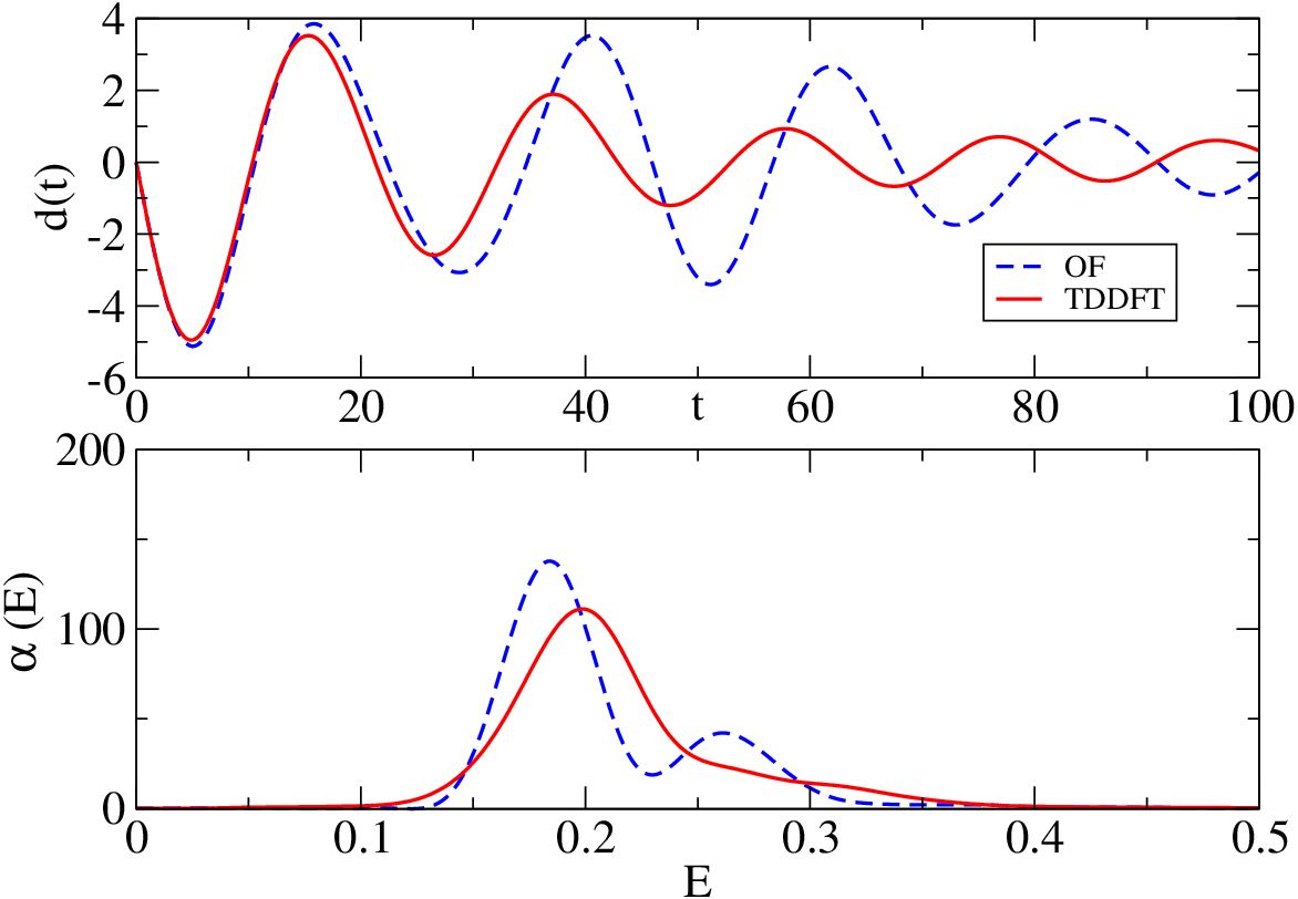
To study the time-dependent behavior of the density in TDDFT and OF in this case we have calculated the time dependence of the dipole moment. To start the calculation the initial ground state wave functions were perturbed by multiplying them with , with a.u. and the systems were time propagated up to a.u. The calculated dipole moment is shown in Fig. 2. The TDDFT and OF dipole moments are very close to each other in the beginning of the calculation, but later the oscillations are different. It seems that the constraining potential works well in the initial stage of the time propagation, but later dynamical effects become important. This can probably be improved by invoking a dynamical kinetic energy potential Neuhauser et al. 2011; Luo et al. 2014. The frequency of the oscillation of the dipole moment remains very similar in the OF and TDDFT calculation and the resulting absorption spectra are similar (see Fig. 2). The usefulness of the OF approach for the calculation of the absorption spectrum of quantum dots using a dynamical kinetic energy functional has been discussed in Refs. Xiang et al. 2014; Xiang et al. 2016.
To test the coupled Maxwell TD-OF calculations we will compare them to coupled Maxwell-TDDFT calculations. First, we will use three test cases from Ref. Covington et al. 2019. In the first case, an electromagnetic pulse excites a jellium sheet. Because the Maxwell equations are linear, the electric field can be written as the sum of an external field and an induced field created by the electron currents, . In this way, the exciting pulse does not need a source and never has to be time propagated because its form is analytic. The external field is given as a Gaussian laser pulse ( in Fig. 3)
| (22) |
Here is the pulse shift, controls the width of the pulse.
To show the time-dependence of the electric field and currents we define the average electric field as
| (23) |
and
| (24) |
where the sum is over grid points that are not in the CAP region. In the figures only the components (for and ), and are shown.
Fig.3a shows the induced currents for coupled and uncoupled cases. In the uncoupled case, the Maxwell equations are not time propagated and . For the coupled case, the Maxwell equations are time propagated and the currents produce an induced field opposite to . It is this induced field that de-excites the electrons and causes the current to fall back to zero. The results of the TDDFT and TD-OF calculations agree up to 4 significant digits for the induced currents and induced fields and one cannot distinguish the results on Fig. 3.

The perfect agreement is very surprising considering that 18 orbitals are time propagated in TDDFT and only one in TD-OF. We will see later that this agreement is mostly due to symmetry of the jellium sheet system. Fig.3.a also shows that in the uncoupled case the system stays in an excited state while in the coupled case the system relaxes to the ground state and the electric current decreases to zero.
In the second test case a sheet of aluminium jellium is irradiated with a laser pulse of the form
| (25) |
The TDDFT and OF currents and induced electric fields are in perfect agreement, up to 3 significant digits. In this case the electric field penetrates the thick Al sheet generating strong currents. Still, the results of the TDDFT calculations with 200 orbitals and the orbital free calculation are the same.

In the third example, a jellium sphere of radius 12.8 a.u. containing 236 electrons is used with a short Gaussian pulse (see Fig. 5). In this case the induced electric field is negligible. The OF and TDDFT currents are very close to each other during the laser pulse, but after the excitation the time dependence of the currents is different. The same system with the longer pulse is shown in Fig. 6. The OF and TDDFT are not in perfect agreement as before, but they are similar and they follow the external pulse with the same delay time. This test shows the role of symmetry comparing a sheet and a spherical jellium system. One can cut the sphere into slices in parallel with the direction of the laser. The currents and density oscillations will be different in each slice depending on their diameter. In the jellium sheet cases the response is the same in each slice. Additionally, the jellium sphere presents a surface which causes reflections of the electron density driven to the surface by the laser field. In the case of TDDFT, there are 118 orbitals with different energies and different reflections. For larger systems the effect of the surface is expected to be smaller.
Next we present examples with atoms. In Figs. 7 and 8 OF and TDDFT calculations of a 32 atom and 96 atom Al sheets are compared. The agreement of the OF and TDDFT results is excellent, the thicker (the width is about 42 a.u.) sheet of 96 atom system has better agreement than the thinner case. This example illustrates that the presence of atomic potentials does not greatly affect the agreement between the OF and TDDFT results.
Finally, we present a calculation for a Al icosahedron cluster. As the TDDFT calculations are computationally demanding, we use a shorter pulse in this case. The coupling to the Maxwell equations is also turned off – partly to increase the speed of the calculation partly because the induced fields are small as we have seen in the jellium case (see Fig. 6. The agreement of the TDDFT and OF calculations is perfect. The reason of the very good agreement is probable due to the localization of the density by the atomic potentials. In the jellium case, the electron density is more easily moved by the field.
IV Summary
We have implemented and tested the coupled Maxwell and TD-OF calculations to study the interaction of electromagnetic fields and matter. Nanometer sized sheets and clusters were subject to short laser pulses and the induced currents and electric fields were compared to the result of TDDFT calculations. The results are in very good agreement, especially for larger systems. The examples and tests include dipole oscillation due to an instantaneous kick perturbation, excitation with a laser field and coupled Maxwell and quantum dynamics. The coupled Maxwell case is a rigorous test because the system does not just follow the dynamics of the laser field but builds up a nonlinear response. This test is also important for possible applications.
The OF calculations have some limitations for smaller quantum dots Ho et al. 2007; Aguado 2001; Aguado et al. 2001 and the disagreement can perhaps be reduced by using more recently proposed kinetic energy functionals Mi and Pavanello 2019; Shao et al. 2020. In these calculations, a constraining potential was used to force the OF ground state density to match the DFT ground state density. This step can probably be eliminated by using new generations of kinetic energy functionals Mi and Pavanello 2019; Shao et al. 2020; Mi et al. 2018; Xu et al. 2019; Mi and Pavanello 2019; Xu et al. 2020.
Another potential improvement is using dynamic kinetic energy potentials Neuhauser et al. 2011; White et al. 2018. These potentials have been tested only in very few cases and further development and tests might be needed.
In the present work the size of the studied systems is relatively small because TDDFT calculations are not feasible for larger systems. The results are promising and larger, physically more relevant systems will be studied in later works.


References
- Hohenberg and Kohn (1964) P. Hohenberg and W. Kohn, Phys. Rev. 136, B864 (1964).
- Kohn and Sham (1965) W. Kohn and L. J. Sham, Phys. Rev. 140, A1133 (1965).
- Goedecker (1999) S. Goedecker, Rev. Mod. Phys. 71, 1085 (1999).
- Bowler and Miyazaki (2012) D. R. Bowler and T. Miyazaki, Reports on Progress in Physics 75, 036503 (2012).
- Wang and Carter (2002) Y. A. Wang and E. A. Carter, in Theoretical Methods in Condensed Phase Chemistry, edited by S. D. Schwartz (Dordrecht, 2002) pp. 117–184.
- Wesolowski and Wang (2013) T. A. Wesolowski and Y. A. Wang, eds., Recent Progress in Orbital-Free Density Functional Theory (World Scientific Publishing Co. Pte. Ltd., Singapore, 2013).
- Karasiev et al. (2014) V. V. Karasiev, D. Chakraborty, and S. Trickey, in Many-Electron Approaches in Physics, Chemistry, and Mathematics, edited by L. Delle Site and V. Bach (Springer, Heidelberg, 2014) pp. 113–134.
- Witt et al. (2018) W. C. Witt, B. G. del Rio, J. M. Dieterich, and E. A. Carter, Journal of Materials Research 33, 777–795 (2018).
- Shao et al. (2018) X. Shao, Q. Xu, S. Wang, J. Lv, Y. Wang, and Y. Ma, Computer Physics Communications 233, 78 (2018).
- Hung and Carter (2009) L. Hung and E. A. Carter, Chemical Physics Letters 475, 163 (2009).
- White et al. (2013) T. G. White, S. Richardson, B. J. B. Crowley, L. K. Pattison, J. W. O. Harris, and G. Gregori, Phys. Rev. Lett. 111, 175002 (2013).
- Ding et al. (2018) Y. H. Ding, A. J. White, S. X. Hu, O. Certik, and L. A. Collins, Phys. Rev. Lett. 121, 145001 (2018).
- Mi and Pavanello (2019) W. Mi and M. Pavanello, Phys. Rev. B 100, 041105 (2019).
- Shao et al. (2020) X. Shao, W. Mi, and M. Pavanello, “New-generation nonlocal orbital-free dft reaches beyond the nanoscale,” (2020), arXiv:2010.07385 [cond-mat.mtrl-sci] .
- Ho et al. (2007) G. S. Ho, C. Huang, and E. A. Carter, Current Opinion in Solid State and Materials Science 11, 57 (2007).
- Aguado (2001) A. Aguado, Phys. Rev. B 63, 115404 (2001).
- Aguado et al. (2001) A. Aguado, J. M. López, J. A. Alonso, and M. J. Stott, The Journal of Physical Chemistry B 105, 2386 (2001).
- Chen et al. (2015) M. Chen, J. Xia, C. Huang, J. M. Dieterich, L. Hung, I. Shin, and E. A. Carter, Computer Physics Communications 190, 228 (2015).
- (19) X. Shao, K. Jiang, W. Mi, A. Genova, and M. Pavanello, WIREs Computational Molecular Science n/a, e1482, https://onlinelibrary.wiley.com/doi/pdf/10.1002/wcms.1482 .
- Golub and Manzhos (2020) P. Golub and S. Manzhos, Computer Physics Communications 256, 107365 (2020).
- Holas and March (1991) A. Holas and N. H. March, Phys. Rev. A 44, 5521 (1991).
- Levämäki et al. (2014) H. Levämäki, A. Nagy, K. Kokko, and L. Vitos, Phys. Rev. A 90, 062515 (2014).
- White et al. (2018) A. J. White, O. Certik, Y. H. Ding, S. X. Hu, and L. A. Collins, Phys. Rev. B 98, 144302 (2018).
- Xiang et al. (2016) H. Xiang, M. Zhang, X. Zhang, and G. Lu, The Journal of Physical Chemistry C 120, 14330 (2016).
- Xiang et al. (2020) H. Xiang, Z. Wang, L. Xu, X. Zhang, and G. Lu, The Journal of Physical Chemistry C 124, 945 (2020).
- Xiang et al. (2014) H. Xiang, X. Zhang, D. Neuhauser, and G. Lu, The Journal of Physical Chemistry Letters 5, 1163 (2014).
- Neuhauser et al. (2011) D. Neuhauser, S. Pistinner, A. Coomar, X. Zhang, and G. Lu, The Journal of Chemical Physics 134, 144101 (2011).
- Levy and Ou-Yang (1988) M. Levy and H. Ou-Yang, Phys. Rev. A 38, 625 (1988).
- Karasiev et al. (2012) V. V. Karasiev, T. Sjostrom, and S. B. Trickey, Phys. Rev. B 86, 115101 (2012).
- Luo et al. (2018) K. Luo, V. V. Karasiev, and S. B. Trickey, Phys. Rev. B 98, 041111 (2018).
- Constantin et al. (2019) L. A. Constantin, E. Fabiano, and F. Della Sala, Journal of Chemical Theory and Computation 15, 3044 (2019).
- Constantin et al. (2018) L. A. Constantin, E. Fabiano, and F. Della Sala, The Journal of Physical Chemistry Letters 9, 4385 (2018).
- Lehtomäki and Lopez-Acevedo (2019) J. Lehtomäki and O. Lopez-Acevedo, Phys. Rev. B 100, 165111 (2019).
- Smargiassi and Madden (1994) E. Smargiassi and P. A. Madden, Phys. Rev. B 49, 5220 (1994).
- Wang and Teter (1992) L.-W. Wang and M. P. Teter, Phys. Rev. B 45, 13196 (1992).
- Perrot (1994) F. Perrot, Journal of Physics: Condensed Matter 6, 431 (1994).
- Chacón et al. (1985) E. Chacón, J. E. Alvarellos, and P. Tarazona, Phys. Rev. B 32, 7868 (1985).
- Wang et al. (1998) Y. A. Wang, N. Govind, and E. A. Carter, Phys. Rev. B 58, 13465 (1998).
- Wang et al. (1999) Y. A. Wang, N. Govind, and E. A. Carter, Phys. Rev. B 60, 16350 (1999).
- Xia and Carter (2012) J. Xia and E. A. Carter, Phys. Rev. B 86, 235109 (2012).
- Mi et al. (2018) W. Mi, A. Genova, and M. Pavanello, The Journal of Chemical Physics 148, 184107 (2018).
- Xu et al. (2019) Q. Xu, Y. Wang, and Y. Ma, Phys. Rev. B 100, 205132 (2019).
- Seino et al. (2019) J. Seino, R. Kageyama, M. Fujinami, Y. Ikabata, and H. Nakai, Chemical Physics Letters 734, 136732 (2019).
- Meyer et al. (2020) R. Meyer, M. Weichselbaum, and A. W. Hauser, Journal of Chemical Theory and Computation 16, 5685 (2020), pMID: 32786898.
- Fujinami et al. (2020) M. Fujinami, R. Kageyama, J. Seino, Y. Ikabata, and H. Nakai, Chemical Physics Letters 748, 137358 (2020).
- Manzhos and Golub (2020) S. Manzhos and P. Golub, The Journal of Chemical Physics 153, 074104 (2020).
- (47) J. Lindhard, Kgl. Danske Videnskab. Selskab Mat.-fys. Medd. .
- Covington et al. (2019) C. Covington, D. Kidd, H. Buckner, H. Appel, and K. Varga, Phys. Rev. E 100, 053301 (2019).
- Runge and Gross (1984) E. Runge and E. K. U. Gross, Phys. Rev. Lett. 52, 997 (1984).
- Varga and Driscoll (2011) K. Varga and J. A. Driscoll, Computational Nanoscience: Applications for Molecules, Clusters, and Solids (Cambridge University Press, 2011).
- Jestädt et al. (2019) R. Jestädt, M. Ruggenthaler, M. J. T. Oliveira, A. Rubio, and H. Appel, Advances in Physics 68, 225 (2019).
- Kidd et al. (2018) D. Kidd, A. S. Umar, and K. Varga, Phys. Rev. B 98, 075108 (2018).
- Perdew and Zunger (1981) J. P. Perdew and A. Zunger, Phys. Rev. B 23, 5048 (1981).
- Huang and Carter (2008) C. Huang and E. A. Carter, Phys. Chem. Chem. Phys. 10, 7109 (2008).
- Doye (2003) J. P. K. Doye, The Journal of Chemical Physics 119, 1136 (2003).
- Luo et al. (2014) K. Luo, J. I. Fuks, E. D. Sandoval, P. Elliott, and N. T. Maitra, The Journal of Chemical Physics 140, 18A515 (2014).
- Xu et al. (2020) Q. Xu, J. Lv, Y. Wang, and Y. Ma, Phys. Rev. B 101, 045110 (2020).