Probabilistic Contrastive Principal Component Analysis

Let $x_{1},\cdots,x_{n}\in\mathbb{R}^{D}$ be i.i.d. observations and $X\in\mathbb{R}^{n\times D}$ with the $i$th row $x_{i}^{\top}$. PCA is designed to find the best $d$-dimensional affine subspace to represent the data, where $d<D$. There are several equivalent definitions of PCA. We review two of them below.

The first definition is derived from a geometric perspective, where PCA finds a hyperplane $V$ that minimizes the distance between the samples and this hyperplane:

$$\underset{V^{\top}V=\Id_{d}}{\argmin}\penalty\ \sum_{i=1}^{n}d^{2}(x_{i},V)=\underset{V^{\top}V=\Id_{d}}{\argmin}\penalty\ \sum_{i=1}^{n}\|x_{i}-VV^{\top}x_{i}\|^{2}=\underset{V^{\top}V=\Id_{d}}{\argmin}\penalty\ \frac{1}{n}\sum_{i=1}^{n}\|x_{i}-VV^{\top}x_{i}\|^{2},$$

(1)

where $V\in\mathbb{R}^{D\times d}$ has orthonormal column(s) , representing a $d$-dimensional subspace of $\mathbb{R}^{D}$. The solution is given by

$$V=[v_{1},\cdots,v_{d}],\penalty\ v_{j}=\mathrm{eig}_{j}\left(\sum_{i=1}^{n}x_{i}x_{i}^{\top}\right)=\mathrm{eig}_{j}(C),$$

where $\eig_{j}$ is the $j$th eigenvalue of $C=\sum_{i=1}^{n}x_{i}x_{i}^{\top}$ in the descending order.

The second definition, which leads to an equivalent solution as Equation (1), is motivated from a statistical perspective. In particular, PCA maximizes the variance of the projected data onto each principal component, subject to the components being orthogonal to one another (assume $d=2$ for simplicity):

$$\max_{v_{1}^{\top}v_{1}=1}\var(v_{1}^{\top}x_{i})=\max_{v_{1}^{\top}v_{1}=1}\penalty\ \sum_{i=1}^{n}v_{1}^{\top}x_{i}x_{i}^{\top}v_{1}=\max_{v_{1}^{\top}v_{1}=1}\penalty\ v_{1}^{\top}Cv_{1},$$

(2)

$$\max_{v_{2}^{\top}v_{2}=1,v_{1}^{\top}v_{2}=0}\var(v_{2}^{\top}(x_{i}-v_{1}v_{1}^{\top}x_{i}))=\max_{v_{2}^{\top}v_{2}=1,v_{1}^{\top}v_{2}=0}v_{2}^{\top}Cv_{2}.$$

(3)

The geometric and statistical frameworks for PCA yield equivalent solutions, but having multiple perspectives gives greater insight into the method. Our work is motivated by these complementary perspectives (Theorem 1).

Note that we drop the mean parameter since, in practice, the data can easily be centered to have zero mean. Thus, for simplicity, throughout this paper we assume all data include features that are centered at zero.

PCA may be generalized in the form of a probabilistic model. Assume $z\sim N(0,\Id_{d})$, $x=Wz+\epsilon$ with $W\in\mathbb{R}^{D\times d}$, $\epsilon\sim N(0,\sigma^{2}\Id_{D})$. Then

$$x\sim N(0,WW^{\top}+\sigma^{2}\Id_{D}).$$

The objective is to maximize the likelihood with respect to the parameters $W$ and $\sigma^{2}$:

$$\underset{W,\sigma^{2}}{\argmax}\penalty\ p(X|W,\sigma^{2}).$$

(4)

The MLE of $W$ and $\sigma^{2}$ are given by (Roweis, 1998; Tipping and Bishop, 1999):

$$\widehat{W}_{ML}=U(\Lambda-\widehat{\sigma}^{2}_{ML}I_{d})^{1/2}R,\penalty\ \penalty\ \widehat{\sigma}^{2}_{ML}=\frac{1}{D-d}\sum_{i=d+1}^{D}\lambda_{i},$$

where $U$ consists of the first $d$ eigenvectors of $C=\sum_{i=1}^{n}x_{i}x_{i}^{\top}$ with eigenvalues $\lambda_{1}\geq\cdots\geq\lambda_{D}>0$, $\Lambda=\diag\{\lambda_{1},\cdots,\lambda_{d}\}$ and $R\in\mathrm{O}(d)$ is any rotation matrix.

That is, the hyperplane obtained by PPCA only differs by a re-scaling of the basis from the PCA hyperplane. In other words, PPCA is “equivalent” to PCA, and this becomes exact when $\sigma^{2}\to 0$.

PCA can also be generalized for contrastive modeling of two datasets. For foreground observations $x_{1},\cdots,x_{n}\in\mathbb{R}^{D}$ and background observations $y_{1},\cdots,y_{m}\in\mathbb{R}^{D}$, contrastive PCA (CPCA, Abid et al., 2018) is designed to discover low-dimensional structure that is unique to or enriched in the foreground dataset $X$ relative to the background dataset $Y$. Let $C_{X}=\frac{1}{n}\sum_{i=1}^{n}x_{i}x_{i}^{\top}$ be the empirical covariance matrix for $X$ and $C_{Y}=\frac{1}{m}\sum_{j=1}^{m}y_{j}y_{j}^{\top}$ for $Y$.

Recall the statistical perspective of PCA given by Equation 2. In the contrastive setting, for any unit vector $v$, we have two variances — the foreground variance and background variance — given by $v^{\top}C_{X}v$ and $v^{\top}C_{Y}v$, respectively. The objective of CPCA is to identify directions $v$ that account for a large amount of variance in the foreground and a small amount of variance in the background. Specifically, CPCA solves the following optimization problem:

$$\underset{v^{\top}v=1}{\argmax}\penalty\ v^{\top}C_{X}v-\gamma v^{\top}C_{Y}v=\underset{v^{\top}v=1}{\argmax}\penalty\ v^{\top}Cv,$$

(5)

where $\gamma\in[0,\infty]$ is a tuning parameter, and $C=C_{X}-\gamma C_{Y}$.

The solution of CPCA is the same as PCA if we replace $C_{X}$ by $C$, namely, the optimal $v$ is the top eigenvector of $C$. From the definition of CPCA, it is clear that CPCA reduces to PCA when $\gamma=0$.

CPCA was originally defined from a statistical perspective (Equation 5, Abid et al., 2018). Recalling the geometric definition of PCA, Equation 1, it is natural to consider whether there also exists a geometric interpretation for CPCA.

In addition to the geometric intuition provided by Theorem 1, this theorem also allows us to adapt distance-based algorithms to the contrastive setting. Specifically, in any of these algorithms, one can consider replacing the distance by the “constrastive distance.” For example, sparse CPCA has been developed following this philosophy (Boileau et al., 2020), although without this justification. However, it is important to note that the contrastive distance is not a well-defined distance, which may violate the assumptions of traditional distance-based algorithms, and so cannot be used to replace distance metrics in existing algorithms without some luck.

Another crucial consideration of CPCA is the positive definiteness of $C$, which may be treated as a “covariance matrix.” However, $C$ is not necessarily positive definite unless $\gamma=0$, in which case $C=C_{X}$.

Here, we derive a sufficient condition on $\gamma$ such that $C$ is positive definite. Let the eigenvalues of $C$, $C_{X}$, and $C_{Y}$ be $\lambda_{1}\geq\cdots\lambda_{D}\geq 0$, $\mu_{1}\geq\cdots\mu_{D}\geq 0$ and $\rho_{1}\geq\cdots\geq\rho_{D}\geq 0$, respectively.

The proof can be found in Appendix 9.3. However, in CPCA, the positive definiteness of $C$ is not strictly required since the target is a $d\ll D$ dimensional subspace, and $D$ is large for high-dimensional data, such as biomedical data. Instead, CPCA only requires that the first $d$ eigenvalues of $C$ must be positive. In many applications for visualization and clustering, $d=2$ (Abid et al., 2018), which allows $\gamma$ to be defined over a wide range.

The following theorem provides a necessary and sufficient condition for the first $d$ eigenvalues of $C$ being positive, with Lemma 1 as a special case when $d=D$.

The proof can be found in Appendix 9.4.

The proof can be found in Appendix 9.5. The above corollary explains why, when $\gamma$ is large, a smaller $d$ is preferable: when $\gamma$ is large enough (such that $\lambda_{3}<0$), CPCA with $d=2$ is better than higher dimensional CPCA in terms of mean squared error (MSE). See Section 6 for more details.

In CPCA, the tuning parameter $\gamma$ can be any non-negative real number, making it difficult to tune. Although a tuning method was suggested in the original CPCA proposal (Abid et al., 2018), the procedure depends on an almost exhaustive search, making it inefficient. We first analyze the role of $\gamma$ and propose a new parameterization such that the new tuning parameter $\gamma$ always lies in a small range, typically close to $[0,1]$, making it easier to tune.

Recall that, for PCA, minimizing the sum of squared error and minimizing the mean squared error are equivalent, since the scale $\frac{1}{n}$ only changes the eigenvalues of the sample covariance, not its eigenvectors:

$$\underset{v^{\top}v=1}{\argmin}\sum_{i=1}^{n}\|x_{i}-vv^{\top}x_{i}\|^{2}=\underset{v^{\top}v=1}{\argmin}\penalty\ \frac{1}{n}\sum_{i=1}^{n}\|x_{i}-vv^{\top}x_{i}\|^{2}.$$

However, in the contrastive setting, the scale matters. Specifically, the following two optimization problems are not equivalent unless $m=n$, which rarely happens in practice:

		$\displaystyle\underset{v^{\top}v=1}{\argmin}\sum_{i=1}^{n}\|x_{i}-vv^{\top}x_{i}\|^{2}-\gamma^{\prime}\sum_{i=1}^{m}\|y_{i}-vv^{\top}y_{i}\|^{2}$		(7)
		$\displaystyle\hskip-17.07182pt\neq\underset{v^{\top}v=1}{\argmin}\penalty\ \frac{1}{n}\sum_{i=1}^{n}\|x_{i}-vv^{\top}x_{i}\|^{2}-\frac{1}{m}\gamma^{\prime}\sum_{i=1}^{m}\|y_{i}-vv^{\top}y_{i}\|^{2}.$

Comparing Equations (6) and (7), we conclude that they are equivalent when $\gamma^{\prime}=\gamma\frac{n}{m}$. If the sample sizes of the two groups are not the same, then the choice of $\gamma$ is different from the choice of $\gamma^{\prime}$. We will show that this reparameterization, which is adjusted by the relative sample size, makes $\gamma$ more interpretable and easier to tune.

As a slightly different model than CPCA, the contrastive latent variable model (CLVM) has been proposed (Severson et al., 2019):

$$z\sim N(0,\Id_{d}),\penalty\ t\sim N(0,\Id_{d^{\prime}}),\penalty\ x=Sz+Wt+\epsilon_{x},\penalty\ y=Sz+\epsilon_{y},\penalty\ \epsilon_{x},\epsilon_{y}\sim N(0,\sigma^{2}\Id_{D}).$$

(8)

The marginals are given by

$$x\sim N(0,SS^{\top}+WW^{\top}+\sigma^{2}\Id_{D}),\penalty\ \penalty\ y\sim N(0,SS^{\top}+\sigma^{2}\Id_{D}).$$

The objective function in inference is the likelihood or log likelihood. When the background dimension is zero, that is, when $d^{\prime}=0$, the above model becomes PPCA for $X\cup Y$.

However, we are interested in characterizing the foreground data $X$ while controlling for variation in the background $Y$. For this reason, it is more desirable to recover PPCA for $X$ as a special case of the model rather than PPCA for $X\cup Y$ or $Y$. Recall that similar a relation holds for PCA and CPCA: when $\gamma=0$, CPCA becomes PCA on $X$ only. In fact, there does not exist any $\gamma$ such that CPCA is equivalent to PCA on $X\cup Y$.

In addition, there is no clear link between the CLVM (Equation 8) and CPCA, even if $\sigma^{2}\to 0$. As a result, it is of interest to develop a general model that is simultaneously a probabilistic version of CPCA and a contrastive version of PPCA.

Consider the following model

$$z_{x},z_{y}\sim N(0,\Id_{d}),\penalty\ x=Wz_{x}+\epsilon_{x},\penalty\ y=Wz_{y}+\epsilon_{y},$$

(9)

where $\epsilon_{x},\penalty\ \epsilon_{y}\sim N(0,\sigma^{2}\Id_{D})$ are i.i.d. Gaussian noise vectors. Recall the equivalent statistical and geometric interpretations of PPCA: maximizing the likelihood of $X$ is equivalent to minimizing the distance between $X$ and the hyperplane $W$. For CPCA, we expect such $W$ to be far away from the background $Y$, which is exactly the (geometric) objective of CPCA (see Theorem 1). In the probabilistic setting, maximizing the distance from $Y$ is equivalent to minimizing the likelihood of $Y$. This is counter-intuitive, but it coincides with our model’s motivation to account for variation in the foreground data, not the background data. Thus, we have the following objective function

$$\underset{W,\sigma^{2}}{\argmax}\penalty\ \frac{p(X|W,\sigma^{2})}{p(Y|W,\sigma^{2})^{\gamma}}.$$

(10)

The above objective function becomes the PPCA objective function when $\gamma=0$, and a relative likelihood when $\gamma=1$. For general $\gamma\in[0,\infty)$, we refer to Equation 10 as the relative likelihood, as it captures the likelihood of the foreground data with respect to the likelihood of the background data, scaled by $\gamma$.

The non-traditional nature of this objective requires further comment. Notice that this objective is not a traditional likelihood ratio, which is typically defined as a ratio of the likelihood of one dataset under two different parameter settings. Rather, ours is a ratio of likelihoods of two different datasets under a shared parameter setting. Furthermore, Equation (10) is not a well-defined likelihood unless $\gamma=0$. These caveats preclude the use of traditional estimation and inference procedures based on likelihoods and relative likelihoods. For this reason, we present alternative procedures: one based on a direct maximization of Equation (10) and another based on generalized posterior inference.

First, we investigate the closed-form solution for this objective.

The proof can be found in Appendix 9.6. As a result, we find last missing piece in the commutative diagram 1, namely, we have a complete algorithm for PCPCA that allows PCA, PPCA, and CPCA to be recovered as subcases of this general framework.

Let $\Theta$ be the space of parameters, which can be a finite or infinite dimensional space, and $U$ be the feature space, then we denote the loss function $l:U\times\Theta\to\mathbb{R}$ and $l_{\theta}:U\to\mathbb{R}$. For a given measure $P$ on $U$ (often the true measure), define the risk function $R:\Theta\to\mathbb{R}$ to be

$$R:\Theta\to\mathbb{R},\penalty\ \theta\mapsto\mathbb{E}_{P}[l_{\theta}].$$

Then the goal is to minimize the risk: $\min_{\theta\in\Theta}R(\theta)$. It is common to assume the minimizer is unique, denoted by $\theta^{*}=\underset{\theta\in\Theta}{\arg\min}\penalty\ R(\theta)$.

However, $P$ is often unknown. Instead, we have observations $u_{1},\cdots,u_{n}$ and we have the corresponding empirical measure $P_{n}=\frac{1}{n}\sum_{i=1}^{n}\delta_{u_{i}}$. Then the empirical risk function is

$$R_{n}:\Theta\to\mathbb{R},\penalty\ \theta\mapsto\mathbb{E}_{P_{n}}[l_{\theta}].$$

The goal in this more practical setting is to minimize the empirical risk:

$$\min_{\theta\in\Theta}R_{n}(\theta).$$

Let $\widehat{\theta}_{n}=\underset{\theta\in\Theta}{\arg\min}\penalty\ R_{n}(\theta)$ be the unique minimizer of the empirical risk.

If a statistical model exists with density function $p_{\theta}$ and the loss function is $l_{\theta}(u)=-\log p_{\theta}(u)$, then this minimization reduces to maximum likelihood estimation. In particular, in this setting, $R_{n}(\theta)$ is the negative log likelihood and $\widehat{\theta}_{n}$ is the MLE.

The Gibbs posterior becomes the true posterior if $R_{n}$ is the negative log-likelihood.

Note that $d$ is only required to be positive semi-definite, that is, $d(\theta;\theta^{\prime})\geq 0$ with equality iff $\theta=\theta^{\prime}$.

We next propose a loss function and Gibbs posterior for CPCA. Let $u=(x,\alpha)$ where $x\in\mathbb{R}^{D}$ is the observation, $\alpha\in\{0,1\}$ with $\alpha=0$ represents foreground data while $\alpha=1$ represents background data and $\theta=V\in\Gr(D,d)$, the Grassmannian manifold. Let the loss function be

$$l_{\theta}(u)=(-\gamma)^{\alpha}d^{2}(x,V)=(-\gamma)^{\alpha}\|x-VV^{\top}x\|^{2}=(-\gamma)^{\alpha}\left(x^{\top}x-xVV^{\top}x\right).$$

For simplicity, assume $u_{1},\cdots,u_{n}$ are foreground data while $u_{n+1},\cdots,u_{n+m}$ are background data. As a result, the empirical risk function is

	$\displaystyle R_{n}(\theta)$	$\displaystyle=\frac{1}{n+m}\sum_{i=1}^{n+m}l_{\theta}(u_{i})$
		$\displaystyle=\frac{1}{n+m}\left(\sum_{i=1}^{n}\left(x_{i}^{\top}x_{i}-x_{i}^{\top}VV^{\top}x_{i}\right)-\gamma\sum_{j=1}^{m}\left(x_{n+j}^{\top}x_{n+j}-x_{n+j}^{\top}VV^{\top}x_{n+j}\right)\right)$
		$\displaystyle=-\sum_{i=1}^{n}x_{i}^{\top}VV^{\top}x_{i}+\gamma\sum_{j=1}^{m}x_{n+j}^{\top}VV^{\top}x_{n+j}+M$
		$\displaystyle=-\operatorname{tr}(VV^{\top}C)+M,$

where $C=\sum_{i=1}^{n}x_{i}x_{i}^{\top}-\gamma\sum_{j=1}^{m}x_{n+j}x_{n+j}^{\top}$ and $M$ is independent of $\theta$. We conclude that the empirical risk function coincides with the objective function of CPCA. Furthermore, if the prior $\Pi$ is chosen to be the uniform prior, then the maximum a posteriori estimation (MAP) matches the solution of CPCA, which is the subspace spanned by the first $d$ eigenvectors of $C$.

For the population version of the risk, assume $P=\beta P_{F}+(1-\beta)P_{B}$ where $\beta\in(0,1)$, $P_{F}$ is the foreground measure with zero mean and covariance $C_{F}$, and $P_{B}$ is the background measure with zero mean and covariance $C_{B}$. Then the risk function is

	$\displaystyle R(\theta)$	$\displaystyle=\mathbb{E}_{P}l_{\theta}(u)$
		$\displaystyle=\beta\mathbb{E}_{x\sim P_{F}}\left(x^{\top}x-x^{\top}VV^{\top}x\right)-(1-\beta)\gamma\mathbb{E}_{x\sim P_{B}}\left(x^{\top}x-x^{\top}VV^{\top}x\right)$
		$\displaystyle=-\beta\operatorname{tr}(VV^{\top}C_{F})-(1-\beta)\gamma\operatorname{tr}(VV^{\top}C_{B})+M$
		$\displaystyle=-\operatorname{tr}(VV^{\top}C)+M,$

where $C=\beta C_{F}-(1-\beta)\gamma C_{B}$ and $M$ is independent of $\theta$. So the minimizer is given by

$$\theta^{*}=V^{*}=[\eig_{1}(C),\cdots,\eig_{d}(C)].$$

We consider the risk divergence $d(\theta;\theta^{*})=(R(\theta)-R(\theta^{*}))^{1/2}=\operatorname{tr}((V^{*}V^{*\top}-VV^{\top})C)^{1/2}$, which measures the difference between risks. We now consider the contraction rate of this Gibbs posterior.

The proof can be found in Appendix 9.7. As a result, the Gibbs posterior will contract to the optimal parameter as the sample size increases, which provides theoretical support for the generalized Bayesian version of CPCA.

We now consider the Gibbs posterior for PCPCA. Let $u=(x,\alpha)$ where $x\in\mathbb{R}^{D}$ is the observation and $\alpha\in\{0,1\}$ indicates the sample’s condition, with $\alpha=0$ representing foreground data while $\alpha=1$ representing background data. As before, let $\theta=(W,\sigma^{2})$ be the parameter. Let the loss function be $l_{\theta}(u)=-(-\gamma)^{\alpha}\log N(v;0,WW^{\top}+\sigma^{2}\Id_{D})$. For simplicity, assume $u_{1},\cdots,u_{n}$ are foreground data while $u_{n+1},\cdots,u_{n+m}$ are background data. As a result, the empirical risk function is

		$\displaystyle R_{n}(\theta)=\frac{1}{n+m}\sum_{i=1}^{n+m}l_{\theta}(u_{i})$
		$\displaystyle=\frac{1}{n+m}\left(\sum_{i=1}^{n}-\log N(x_{i};0,WW^{\top}+\sigma^{2}\Id_{d})+\gamma\sum_{j=1}^{m}\log N(x_{n+j};0,WW^{\top}+\sigma^{2}\Id_{d})\right)$
		$\displaystyle=\sum_{i=1}^{n}\left(\frac{1}{2}\log|A|+\frac{1}{2}x_{i}^{\top}A^{-1}x_{i}\right)+\gamma\sum_{j=1}^{m}\left(-\frac{1}{2}\log|A|-\frac{1}{2}x_{n+j}^{\top}A^{-1}x_{n+j}\right)+M$
		$\displaystyle=\frac{n-\gamma m}{2}\log|A|+\frac{1}{2}\operatorname{tr}(A^{-1}C)+M,$

where $A=WW^{\top}+\sigma^{2}\Id_{D}$, $C=\sum_{i=1}^{n}x_{i}x_{i}^{\top}-\gamma\sum_{j=1}^{m}x_{n+j}x_{n+j}^{\top}$ and $M$ is independent of $\theta$. We conclude that the empirical risk function coincides with the (negative log) objective function of PCPCA. Furthermore, if the prior $\Pi$ is chosen to be the uniform prior, then the maximum a posteriori (MAP) estimate matches the solution in Theorem 3.

For the population version of the risk, assume the same model as in the previous section. Specifically, we assume $P=\beta P_{F}+(1-\beta)P_{B}$ where $\beta\in(0,1)$, $P_{F}$ is the foreground measure with zero mean and covariance $C_{F}$, and $P_{B}$ is the background measure with zero mean and covariance $C_{B}$. Then the risk function is

	$\displaystyle R(\theta)$	$\displaystyle=\mathbb{E}_{P}l_{\theta}(u)$
		$\displaystyle=-\beta\mathbb{E}_{x\sim P_{F}}\log p(x|0,A)+(1-\beta)\gamma\mathbb{E}_{x\sim P_{B}}\log p(x|0,A)$
		$\displaystyle=\frac{\beta}{2}\left(\log|A|+\operatorname{tr}(A^{-1}C_{F})\right)-\frac{(1-\beta)}{2}\gamma\left(\log|A|+\operatorname{tr}(A^{-1}C_{B})\right)+M$
		$\displaystyle=\frac{\beta-(1-\beta)\gamma}{2}\log|A|+\frac{1}{2}\operatorname{tr}(A^{-1}C)+M,$		(11)

where $C=\beta C_{F}-(1-\beta)\gamma C_{B}$. So the minimizer is given by

$${\sigma^{*2}}=\frac{1}{D-d}\sum_{i=d+1}^{D}\lambda_{i},W^{*}=U_{d}\left(\frac{\Lambda_{d}}{\beta-(1-\beta)\gamma}-\sigma^{*2}\Id\right)^{1/2}R$$

(12)

where $\Lambda_{d}=\diag\{\lambda_{i}\}$ consists of the largest $d$ eigenvalues of $C$, and $U_{d}$ consists of the corresponding $d$ eigenvectors. We consider the same risk divergence as in the previous section:

$$d(\theta;\theta^{*})=(R(\theta)-R(\theta^{*}))^{1/2}=\left(\frac{\beta-(1-\beta)\gamma}{2}(\log|A|-\log|A^{*}|)+\frac{\operatorname{tr}((A^{-1}-A^{*-1})C)}{2}\right)^{1/2}.$$

We now consider the contraction rate of the PCPCA Gibbs posterior under this divergence.

The proof can be found in Appendix 9.8. As a result, the Gibbs posterior contracts to the optimal parameter as the sample size increases, which supports the generalized Bayesian PCPCA.

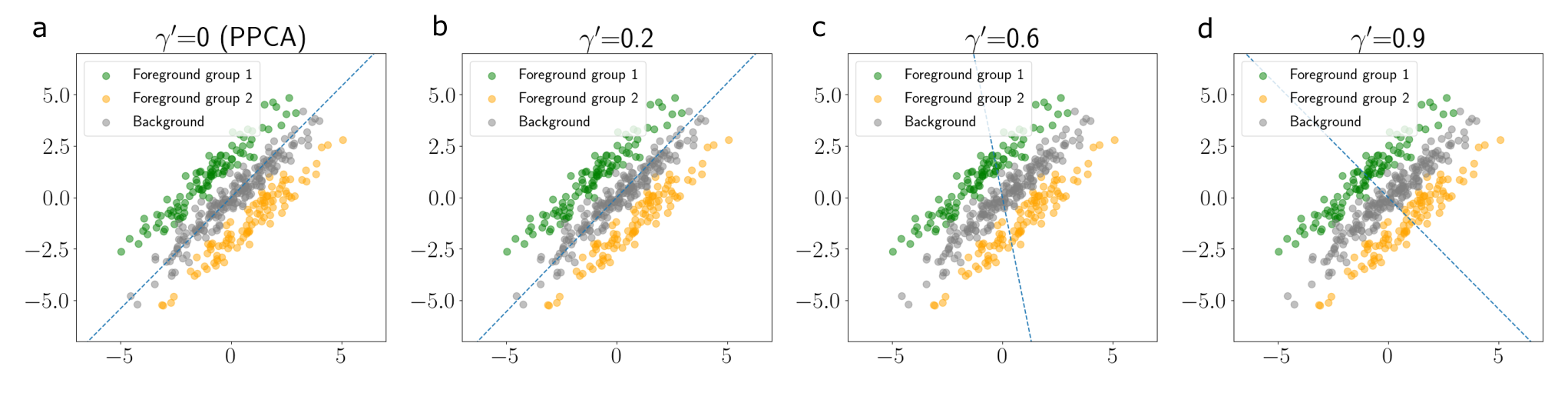
First, to demonstrate the role of the hyperparameter $\gamma$ in the PCPCA model, we fit the PCPCA model on a two-dimensional simulated dataset. In this simple dataset, the foreground data contain two subgroups, each of which shares an axis of variation with the background data. In particular, we generated the foreground and background by sampling $x_{i}\sim\mathcal{N}(\mu_{x},\Sigma)$ and $y_{j}\sim\mathcal{N}(0,\Sigma)$ where $\mu_{x}=\left(\begin{smallmatrix}1\\ -1\end{smallmatrix}\right)$ for half of the foreground samples, and $\mu_{x}=\left(\begin{smallmatrix}-1\\ 1\end{smallmatrix}\right)$ for the other half. For all samples, $\Sigma=\left(\begin{smallmatrix}2.7&2.6\\ 2.6&2.7\end{smallmatrix}\right)$. We set the foreground and background sample sizes to be equal, $n=m=200$. We fit the PCPCA model for $\gamma^{\prime}\in\{0,0.2,0.6,0.9\}$, and we visualize the 1-dimensional line defined by $\widehat{W}_{ML}$, where $d=1$ and $D=2$ (Figure 2).

Recall that when $\gamma^{\prime}=0$, PCPCA reduces to PPCA. In this case, $W$ captures the variation that is shared between the background and foreground data (Figure 2a). At higher values of $\gamma^{\prime}$, we observed that PCPCA captures the variation that is unique to the foreground dataset, which divides the two foreground subgroups (Figure 2d). Note that $\widehat{W}_{ML}$ rotates nearly 90 degrees to capture the direction of maximal variation unique to the foreground data when $\gamma^{\prime}=0.9$ relative to the PPCA solution when $\gamma^{\prime}=0$. At intermediate values of $\gamma^{\prime}$, $\widehat{W}_{ML}$ balances between capturing the shared and foreground-specific variation (Figure 2c).

An advantage of PCPCA’s model-based approach to contrastive learning is its ability to explicitly account for noise in the data. To test this directly, we again fit PCPCA and CPCA to the mouse protein expression dataset, but this time we injected additive, independent Gaussian noise across the features. In particular, we transformed every foreground and background sample $x_{i}$ and $y_{j}$ as

	$\displaystyle\widetilde{x}_{i}$	$\displaystyle=x_{i}+\epsilon_{i}$
	$\displaystyle\widetilde{y}_{j}$	$\displaystyle=y_{j}+\epsilon_{j},$

where $\epsilon_{i},\epsilon_{j}\sim\mathcal{N}(0,\sigma^{2}I_{D})$. We generated ten datasets for $\sigma^{2}\in\{0.5,1,\dots,5\}$. We also included the case when $\sigma^{2}=0$, which is the original dataset with no additional noise.

We fit PCPCA and CPCA on each of these noisy datasets and measured the silhouette score of PCPCA and CPCA with $d=2$. We repeated this experiment $100$ times for each value of $\sigma^{2}$. We tuned $\gamma$ independently for PCPCA and CPCA for each value of $\sigma^{2}$ and took the $\gamma$ with the highest silhouette score. We found that, while the performance of both methods declined with more noise, PCPCA showed better performance than CPCA at higher noise levels (Figure 7). This suggests that PCPCA is more robust to noise than CPCA, demonstrating another advantage of our model-based approach.

Another advantage of PCPCA’s model-based approach is the ability to generate data from the foreground data distribution. In CPCA, this is not possible because there is no associated generative model. Note that, in PCPCA, we cannot reasonably generate data from the background distribution because the objective function is a relative likelihood with the goal of minimizing the relative likelihood of the background model. This is not a problem in most settings, as we are typically interested in exploring the variance unique to the foreground data.

To demonstrate PCPCA’s ability to generate realistic foreground data, we used the corrupted MNIST dataset (Abid et al., 2018). In this dataset, the foreground samples are MNIST digits (0s and 1s) superimposed onto natural images of grass from ImageNet (Russakovsky et al., 2015). The background samples are unaltered natural images of grass (Figure 8).

We fit PCPCA with $d=2$ and $\gamma^{\prime}=0.8$ to obtain $\widehat{W}_{ML}$. For comparison, we also fit PPCA ($\gamma^{\prime}=0$). Examining the latent variables, we found that PCPCA showed substantially better clustering of the two MNIST digits than PPCA — the silhouette score for PCPCA was 0.33, while the score for PPCA was just 0.007 (Figure 9a, c).

To generate new data, we sampled $S=300$ i.i.d. latent variables $z_{s}\sim\mathcal{N}(0,I_{d})$ for $s=1,\dots,S$, and projected these to the data space to obtain synthetic images. Specifically, each generated image is computed as $\widehat{x}_{s}=\widehat{W}_{ML}z_{s}+\mu_{x}$ where $\mu_{x}$ is the mean of the foreground data. We found that these samples recovered the variation in the MNIST digits in the foreground data (Figure 9d). In contrast, samples generated from PPCA did not show as much of the digit structure (Figure 9b). These results suggest that PCPCA can generate realistic data from the foreground distribution, which is useful for exploratory data analysis.

Furthermore, using $\widehat{W}_{ML}$ estimated for PPCA and PCPCA fit to the corrupted MNIST data, we computed the log likelihood of a set of held-out samples of MNIST digits without any corruption. We found that PCPCA has a higher test likelihood than PPCA on these uncorrupted digits (Figure 10). This suggests that the foreground model for PCPCA more accurately captures the uncorrupted MNIST digits relative to PPCA.

We next sought to numerically evaluate the Gibbs posterior for PCPCA. To estimate the posterior, any sampling-based inference methods can be applied. We use the No U-Turn Sampler (Hoffman and Gelman, 2014) — which is an extension of Hamiltonian Monte Carlo — as implemented in the Stan programming language (Carpenter et al., 2017). We place uniform priors on $W$ and $\sigma^{2}$, as required by our theoretical results.

Assume some elements of both the background and foreground matrices are missing. Let $x=[x^{o},x^{u}]^{\top}$, where $x^{o}$ is the sub-vector of observed features and $x^{u}$ unobserved, and $y=[y^{o},y^{u}]$ with the same partition. Consider the missing-at-random setting, where the MLE of the complete data is the same as the MLE of the non-missing data only. Let $x_{i}^{o}$ be the observed subvector of $x_{i}$ with length $D_{i}$, where the locations observed are $i_{1},\cdots,i_{D_{i}}$. Then, we introduce a indicator matrix $L_{i}$ with dimension $D_{i}\times D$ such that $x_{i}^{o}=L_{i}x_{i}$:

$$(L_{i})_{kl}=\begin{cases}1&l=i_{k}\\ 0&\text{otherwise}.\end{cases}$$

Similarly, let $y_{j}^{o}$ be the observed subvector of $y_{j}$ with length $E_{j}$, and define $M_{j}\in\mathbb{R}^{E_{j}\times D}$ as before such that $y_{j}^{o}=M_{j}y_{j}$. Observe that

$$x_{i}^{o}\sim N(0,A_{i}),\penalty\ \penalty\ y_{j}^{o}\sim N(0,B_{j}),\penalty\ \penalty\ A_{i}\coloneqq L_{i}(WW^{\top}+\sigma^{2}\Id_{D})L_{i}^{\top},\penalty\ \penalty\ B_{j}\coloneqq M_{j}(WW^{\top}+\sigma^{2}\Id_{D})M_{j}^{\top}.$$

As a result, the objective function of the observed data is

		$\displaystyle l(W,\sigma^{2})=l(X^{o}|W,\sigma^{2})-\gamma l(Y^{o}|W,\sigma^{2})$
		$\displaystyle=-\frac{1}{2}\sum_{i=1}^{n}\left(D_{i}\log(2\pi)+\log\det(A_{i})+\operatorname{tr}(A_{i}^{-1}x_{i}^{o}{x_{i}^{o}}^{\top})\right)+\frac{\gamma}{2}\sum_{j=1}^{m}\left(E_{i}\log(2\pi)+\log\det(B_{j})+\operatorname{tr}(B_{j}^{-1}y_{j}^{o}{y_{j}^{o}}^{\top})\right).$

Then we take the derivative w.r.t. to $W$:

$\displaystyle\frac{\partial l}{\partial W}$

$\displaystyle=-\left\{\sum_{i=1}^{n}L_{i}^{\top}A_{i}^{-1}\left(\Id_{D_{i}}-x_{i}^{o}{x_{i}^{o}}^{\top}A_{i}^{-1}\right)L_{i}-\gamma\sum_{j=1}^{m}M_{j}^{\top}B_{j}^{-1}\left(\Id_{E_{j}}-y_{j}^{o}{y_{j}^{o}}^{\top}B_{j}^{-1}\right)M_{j}\right\}W.$

Similarly, the derivative w.r.t. $\sigma^{2}$ is

	$\displaystyle\frac{\partial l}{\partial\sigma^{2}}$	$\displaystyle=-\frac{1}{2}\sum_{i=1}^{n}\left(\operatorname{tr}(A_{i}^{-1}L_{i}L_{i}^{\top})-\operatorname{tr}(A_{i}^{-1}x_{i}^{o}{x_{i}^{o}}^{\top}A_{i}^{-1}L_{i}L_{i}^{\top})\right)$
		$\displaystyle\penalty\ \penalty\ \penalty\ +\frac{\gamma}{2}\sum_{j=1}^{m}\left(\operatorname{tr}(B_{j}^{-1}M_{j}M_{j}^{\top})-\operatorname{tr}(B_{j}^{-1}y_{j}^{o}{y_{j}^{o}}^{\top}B_{j}^{-1}M_{j}M_{j}^{\top})\right).$

We can then use iterative optimization algorithms, such as gradient descent, to find $\widehat{W}_{ML}$ and $\widehat{\sigma}^{2}_{ML}$.

References

- Abid et al., (2017) Abid, A., Zhang, M. J., Bagaria, V. K., and Zou, J. (2017). Contrastive principal component analysis. arXiv preprint arXiv:1709.06716.
- Abid et al., (2018) Abid, A., Zhang, M. J., Bagaria, V. K., and Zou, J. (2018). Exploring patterns enriched in a dataset with contrastive principal component analysis. Nature Communications, 9(1):1–7.
- Anderson, (1962) Anderson, T. W. (1962). An introduction to multivariate statistical analysis. Technical report, Wiley New York.
- Boileau et al., (2020) Boileau, P., Hejazi, N. S., and Dudoit, S. (2020). Exploring high-dimensional biological data with sparse contrastive principal component analysis. Bioinformatics, 36(11):3422–3430.
- Brenner et al., (2000) Brenner, N., Bialek, W., and Van Steveninck, R. d. R. (2000). Adaptive rescaling maximizes information transmission. Neuron, 26(3):695–702.
- Candès et al., (2011) Candès, E. J., Li, X., Ma, Y., and Wright, J. (2011). Robust principal component analysis? Journal of the ACM, 58(3):1–37.
- Carpenter et al., (2017) Carpenter, B., Gelman, A., Hoffman, M. D., Lee, D., Goodrich, B., Betancourt, M., Brubaker, M. A., Guo, J., Li, P., and Riddell, A. (2017). Stan: a probabilistic programming language. Grantee Submission, 76(1):1–32.
- Darbyshire and Hamish, (2016) Darbyshire, J. and Hamish, J. (2016). The pricing and hedging of interest rate derivatives: A practical guide to swaps.
- Fruchter, (1954) Fruchter, B. (1954). Introduction to factor analysis. Van Nostrand.
- Hastie and Stuetzle, (1989) Hastie, T. and Stuetzle, W. (1989). Principal curves. Journal of the American Statistical Association, 84(406):502–516.
- Higuera et al., (2015) Higuera, C., Gardiner, K. J., and Cios, K. J. (2015). Self-organizing feature maps identify proteins critical to learning in a mouse model of down syndrome. PloS One, 10(6):e0129126.
- Hoffman and Gelman, (2014) Hoffman, M. D. and Gelman, A. (2014). The no-u-turn sampler: adaptively setting path lengths in hamiltonian monte carlo. J. Mach. Learn. Res., 15(1):1593–1623.
- Hotelling, (1933) Hotelling, H. (1933). Analysis of a complex of statistical variables into principal components. Journal of Educational Psychology, 24(6):417.
- Jirsa et al., (1994) Jirsa, V. K., Friedrich, R., Haken, H., and Kelso, J. S. (1994). A theoretical model of phase transitions in the human brain. Biological Cybernetics, 71(1):27–35.
- Kingma and Ba, (2014) Kingma, D. P. and Ba, J. (2014). Adam: A method for stochastic optimization. arXiv preprint arXiv:1412.6980.
- Lawrence, (2003) Lawrence, N. (2003). Gaussian process latent variable models for visualisation of high dimensional data. Advances in Neural Information Processing Systems, 16:329–336.
- Novembre and Stephens, (2008) Novembre, J. and Stephens, M. (2008). Interpreting principal component analyses of spatial population genetic variation. Nature Genetics, 40(5):646–649.
- Pasini, (2017) Pasini, G. (2017). Principal component analysis for stock portfolio management. International Journal of Pure and Applied Mathematics, 115(1):153–167.
- Rousseeuw, (1987) Rousseeuw, P. J. (1987). Silhouettes: a graphical aid to the interpretation and validation of cluster analysis. Journal of Computational and Applied Mathematics, 20:53–65.
- Roweis, (1998) Roweis, S. T. (1998). EM algorithms for PCA and SPCA. In Advances in Neural Information Processing Systems, pages 626–632.
- Russakovsky et al., (2015) Russakovsky, O., Deng, J., Su, H., Krause, J., Satheesh, S., Ma, S., Huang, Z., Karpathy, A., Khosla, A., Bernstein, M., et al. (2015). Imagenet large scale visual recognition challenge. International Journal of Computer Vision, 115(3):211–252.
- Schölkopf et al., (1998) Schölkopf, B., Smola, A., and Müller, K.-R. (1998). Nonlinear component analysis as a kernel eigenvalue problem. Neural Computation, 10(5):1299–1319.
- Severson et al., (2019) Severson, K. A., Ghosh, S., and Ng, K. (2019). Unsupervised learning with contrastive latent variable models. In Proceedings of the AAAI Conference on Artificial Intelligence, volume 33, pages 4862–4869.
- Syring and Martin, (2020) Syring, N. and Martin, R. (2020). Gibbs posterior concentration rates under sub-exponential type losses. arXiv preprint arXiv:2012.04505.
- Tibshirani, (1996) Tibshirani, R. (1996). Regression shrinkage and selection via the lasso. Journal of the Royal Statistical Society: Series B, 58(1):267–288.
- Tipping and Bishop, (1999) Tipping, M. E. and Bishop, C. M. (1999). Probabilistic principal component analysis. Journal of the Royal Statistical Society: Series B, 61(3):611–622.
- Twine et al., (2011) Twine, N. A., Janitz, K., Wilkins, M. R., and Janitz, M. (2011). Whole transcriptome sequencing reveals gene expression and splicing differences in brain regions affected by alzheimer’s disease. PloS One, 6(1):e16266.
- Vidal et al., (2005) Vidal, R., Ma, Y., and Sastry, S. (2005). Generalized principal component analysis (GPCA). IEEE Transactions on Pattern Analysis and Machine Intelligence, 27(12):1945–1959.
- Young et al., (2018) Young, M. D., Mitchell, T. J., Braga, F. A. V., Tran, M. G., Stewart, B. J., Ferdinand, J. R., Collord, G., Botting, R. A., Popescu, D.-M., Loudon, K. W., et al. (2018). Single-cell transcriptomes from human kidneys reveal the cellular identity of renal tumors. Science, 361(6402):594–599.
- Zheng et al., (2017) Zheng, G. X., Terry, J. M., Belgrader, P., Ryvkin, P., Bent, Z. W., Wilson, R., Ziraldo, S. B., Wheeler, T. D., McDermott, G. P., Zhu, J., et al. (2017). Massively parallel digital transcriptional profiling of single cells. Nature Communications, 8(1):1–12.
- Zou and Hastie, (2005) Zou, H. and Hastie, T. (2005). Regularization and variable selection via the elastic net. Journal of the Royal Statistical Society: Series B, 67(2):301–320.
- Zou et al., (2006) Zou, H., Hastie, T., and Tibshirani, R. (2006). Sparse principal component analysis. Journal of Computational and Graphical tatistics, 15(2):265–286.
- Zou et al., (2013) Zou, J. Y., Hsu, D. J., Parkes, D. C., and Adams, R. P. (2013). Contrastive learning using spectral methods. Advances in Neural Information Processing Systems, 26:2238–2246.
9 Appendix
9.1 Data availability
All data are available via their respective papers. Preprocessing scripts are included in the code repository: https://github.com/andrewcharlesjones/pcpca.
9.2 Proof of Theorem 1
9.3 Proof of Lemma 1
Proof.
Let and be the eigenvalues of and in descending order. Assume ; then for any unit vector with ,
so is positive definite.
Assume with corresponding eigenvectors and where . Let with , then
So is not positive definite.
∎
Note that the second half of the proof is the worst case, where the last eigenvector of matches the first eigenvector of . In order to make positive definite (PD), the strong condition is necessary. However, in practice, much larger values of are sometimes allowed such that is still PD.
9.4 Proof of Theorem 2
Recall that the eigenvalues of , and are , and . Then the eigenvalues of are . Since , by Weyl’s inequalities, for any ,
Similar to the proof of Lemma 1, if the condition is violated, there exists a such that the first eigenvalues are negative. ∎
9.5 Proof of Corollary 1
By the same proof as the proof for the PCA loss, the CPCA loss is . For a fixed , we first show that increasing will result in a smaller . Let , and . Then is positive definite, hence the eigenvalues of are greater than those of . This implies that increasing will decrease the loss.
Then, for a fixed , Theorem 1 implies , so raising to results in a smaller tail sum of the eigenvalues, hence a smaller loss. ∎
9.6 Proof of Theorem 3
First, we find the maximizer of given . Recall the marginals: , and denote . Then, taking the log of the objective function, we have
We drop all constants and the log likelihood becomes
Denote where and . Then, we take the derivative of :
Letting , we have
that is, . solves this equation, that is,
Assume , then
where consists of the first eigenvectors of , contains the corresponding eigenvalues, and is any rotation matrix.
Next, we consider . Plugging into the objective, we have
where . The derivative of is:
Letting , we have so the MLE of is given by
We next connect PCPCA to CPCA and PPCA. When , the objective function (10) is the same as the objective of PPCA, so the MLEs are also the same. Alternatively, when ,
is exactly the solution of CPCA with the new parameterization, which corresponds to eigenvectors of , and is equivalent to the CPCA proposed by Abid et al., 2018 with . In this sense, our parameterization is more natural since it corresponds to the likelihood function.
9.7 Proof of Theorem 4
First recall the following Lemma.
Definition 3.
The the loss function is said to be of sub-exponential type if there exists such that for any ,