FBSDE based neural network algorithms for high-dimensional quasilinear parabolic PDEs
Summary
In this paper, we propose forward and backward stochastic differential equations (FBSDEs) based deep neural network (DNN) learning algorithms for the solution of high dimensional quasilinear parabolic partial differential equations (PDEs), which are related to the FBSDEs by the Pardoux-Peng theory. The algorithms rely on a learning process by minimizing the pathwise difference between two discrete stochastic processes, defined by the time discretization of the FBSDEs and the DNN representation of the PDE solutions, respectively. The proposed algorithms are shown to generate DNN solutions for a 100-dimensional Black–Scholes–Barenblatt equation, accurate in a finite region in the solution space, and has a convergence rate similar to that of the Euler–Maruyama discretization used for the FBSDEs. As a result, a Richardson extrapolation technique over time discretizations can be used to enhance the accuracy of the DNN solutions. For time oscillatory solutions, a multiscale DNN is shown to improve the performance of the FBSDE DNN for high frequencies.
1 Introduction
The relationship between stochastic processes and the solution of partial differential equations represents one of the high achievements of probability theory in potential theory research [1], represented by the celebrated Feynman–Kac formula in linear parabolic and elliptic PDEs as a result of the Kolmogorov backward equation for the generator of the stochastic process for the former [10] and the Dynkin formula for the latter [8]. The recent work by Pardoux–Peng [9] has extended the concept of the classic linear Feynman–Kac formula to a nonlinear version, which connects the solution of a quasilinear parabolic PDE to a coupled pair of forward and backward stochastic processes. This extraordinary development has made much impact in the mathematical finance in option pricing [4].
Meanwhile, in the field of scientific computing, this connection between SDEs and quasilinear PDEs has inspired new approaches of solving high dimensional parabolic partial differential equations (PDEs), which are ubiquitous in material sciences such as the Allen–Cahn equation for phase transition, and quantum mechanics such as the Schrodinger equation as well as the Black–Scholes equation for option pricing and the Hamilton-Jacobi-Bellman equation for optimal control. For PDEs in high dimensions, the main challenge of the traditional numerical methods, such as finite element, finite difference and spectral methods, is the curse of dimensionality, namely, the number of the unknowns in the discretized systems for the PDEs grows exponentially in terms of the dimension of the problem. Recently, machine learning approaches based on the deep neural network have taken advantage of the Pardoux–Peng’s theory for forward and backward stochastic differential equations (FBSDEs) and PDEs. The solution to the PDEs can be learned by sampling the paths of involved stochastic processes, which are discretized in time by the classic Euler–Maruyama scheme [6]. The first such an attempt was done in [2], where neural network was used as an approximator to the gradient of the PDEs solutions, while the PDE’s solution follows the dynamics of the FBSDEs, and the learning was carried out by imposing the terminal condition provided by the parabolic PDEs. Another approach [11] is to approximate the PDE’s solution itself by a deep neural network, which also provides the gradient of the solution as required by the FBSDEs, the learning is then carried out by minimizing the difference between the solution given by the discretized SDEs and that given by the DNN at all discretization time stations. In this paper, improved learning schemes will be proposed based on a similar approach in [11], but with clearer mathematical reasoning for the learning processes, to ensure the numerical methods’ mathematical consistency and improved convergence for the PDEs’ solutions.
The rest of the paper is organized as follows. In Section 2, we will review the Pardoux–Peng’s theory, which establishes the relation between FBSDEs and quasilinear parabolic PDEs, with an emphasis on the relation between the classic Feynman–Kac formula and the nonlinear version represented by the Pardoux–Peng theory. Section 3 will first review the algorithms proposed in [2] and [11], and then two new improved methods will be proposed. Section 4 will present numerical results of the new schemes for solving a 100-dimensional Black–Scholes–Barenblatt equation. Enhanced numerical accuracy by Richardson extrapolations and multi-scale DNNs for PDEs with oscillatory solutions in time will also be discussed. Finally, a conclusion will be given in Section 5.
2 Pardoux–Peng theory on FBSDEs and quasilinear parabolic PDEs
In this paper, we consider the scalar solution , for the following -dimensional parabolic PDE
| (1) |
with a terminal condition
| (2) |
where , , are functions with ranges in with dimensions , and , respectively. We are interested in finding the initial value given . Therefore, in some sense our problem is similar to a time reverse problem for a time reversed version of 1 with an initial data at .
Following Pardoux–Peng in [9], under certain regularity conditions, the forward-backward SDE reformulation gives a nonlinear implicit Feynman–Kac formula for the solution of the parabolic PDE (1). The FBSDEs are proposed as follows. Let where each is a standard Brownian motion. Let be its natural filtration on the time interval . Then, we have the equations of stochastic processes , and in , and dimensions that are adaptive to the filtration , respectively,
| (3) | ||||
| (4) | ||||
If and do not explicitly depend on or , the FBSDEs are decoupled.
By using the Ito’s formula [8] and the forward SDE of , we have
| (6) |
which gives the PDE (1) by comparing (6) with the backward SDE (4) for .
The determination of the third stochastic process from the two SDEs in (3) and (4) makes use of the martingale representation theory [5]. Consider the following special case of the backward SDE (4) as an example:
| (7) |
i.e. , and is the identity matrix. By taking the conditional expectation with respect to , we have
| (8) |
Next, we define the following martingale
| (9) |
where . By the martingale representation theorem [5], there exists a process such that
| (10) |
The stochastic process is unique in the sense that
| (11) |
Meanwhile, we can show that solves the backward SDE (7),
Connection with the classic Feynman–Kac formula is interpreted as follows. If in the parabolic PDE (1), has a linear dependence on , i.e.
| (12) |
then, the backward SDE (4) has an explicit solution
| (13) |
By taking the conditional expectation on both sides, we arrive at
| (14) |
For , using as the initial condition of the forward SDE (3) on the time interval instead of , the traditional Feynman–Kac formula [8] is recovered,
| (15) |
For a general parabolic equation with a nonlinear function , we have
and for given , the following nonlinear equation for is obtained
| (16) |
3 FBSDE based neural network algorithms for quasilinear parabolic PDEs
The learning of the solution will be based on the sample paths of the FBSDEs, which are linked to the PDE solution in (5). Paths of the FBSDEs will be produced by a time discretization algorithm with samples of the Brownian motion .
Let be a uniform partition of . On each interval , define time and Brownian motion increments as
| (17) |
Denoting , and by , and respectively, and applying the Euler–Maruyama scheme to the FBSDEs (3) and (4), respectively, we have
| (18) | ||||
| (19) |
Due to the relationship with the parabolic PDE, the solution to the parabolic PDE provides an alternative representation for and ,
| (20) | ||||
| (21) |
In this paper, fully connected networks of hidden layers will be used, which are given in the following form,
| (22) |
where and are the weight matrices and bias unknowns,respectively, denoted collectively by , , to be optimized via the training, is the activation function and is the application of the activation function applied to a vector quantity component-wisely.
3.1 Existing FBSDE based neural network algorithms
3.1.1 Deep BSDE [2]
The Deep BSDE trains a network to approximate the random value at time , where is the input. are trainable variables and is the targeted quantity of the algorithm. can be obtained similarly as before. The algorithm can be organized as follows.
- 1.
The initial value is given. Trainable variables and are randomly initialized.
- 2.
On each time interval , use the Euler–Maruyama scheme to calculate and as in (18) and (19). Then, train a fully connected feedforward network
(23) where is a fully connected neural network of hidden layers of the form given in (22). Activation functions including ReLU, Tanh, Sigmoid, etc. can been used.
- 3.
Connect all quantities (subnetworks , etc) at to form a network that outputs , which is expected to be an approximation of .
- 4.
The loss function is then defined by a Monte Carlo approximation of
(24)
The Deep BSDE has been shown to give convergent numerical results for various high dimensional parabolic equations [2] and a posteriori estimate suggests strong convergence of half order [3].
Remark 1. The Deep BSDE method from [2] trains the network for the specific initial data and yield only an approximation to the PDE solution . Therefore, once the desired initial data is changed, a new training may have to be carried out. Also, the total size of individual sub-networks used to approximate , will grow linearly in terms of time discretization steps , resulting in large amount of training parameter if higher accuracy of the PDE solution is desired.
3.1.2 FBSNNs [11] (Scheme 1)
The FBSNNs trains a network that directly approximates the solution to the PDE (1) in some region in the space. The network has a fixed size of number of hidden layers and neurons per layer. The algorithm can be organized as follows.
- 1.
The initial value is given. Evaluate and using the network
(25) The gradient above is calculated by an automatic differentiation.
- 2.
- 3.
The loss function is taken as a Monte Carlo approximation of
(28) In this paper, we will name the above numerical method Scheme 1. In order to compare the training results using different values of , the loss function for Scheme 1 is modified as
(29) where serves as the batch size of the training and denotes any instance of sampling of the discretized Brownian motion , and , are the penalty parameters for the terminal conditions. The averaging factor is introduced for consistency consideration as the reduction of the loss function as increases, when applied to the exact solution, is expected.
Remark 2. The FBSNNs algorithm proposed in [11] relies on a loss function involving the difference between sequences and , which carry the information inside the time interval . While the discrete stochastic process can be expected to approach a continuous stochastic process as defined in the backward SDE (4), the question whether the discrete sequence of random variables will converge to the same stochastic process is not clear. As a result, the rate and extent for the difference between and , thus the loss function, approaching to zero is not certain. Our numerical test will provide some evidence for this concern.
3.2 Improved FBSDE based deep neural network algorithms for quasilinear parabolic PDEs
In this section, we propose improved algorithms for the FBSDEs based deep neural networks similar to the approach in [11], but are mathematically consistent in the definition of the loss function and the discretization of both forward and backward SDEs related to the PDE solutions. Specifically, the loss will be made of the difference of two discrete stochastic processes, which will approach the same process given by the backward SDEs if the overall scheme converges.
3.2.1 FBSDE based algorithms - Scheme 2
Based on the Remark 2 from Section 3.1.2, we would like to design a new scheme whose loss function is expected to show the strong convergence rate of the Euler–Maruyama scheme for the discretization of the FBSDEs. A key factor will be to make the loss function as the pathwise differences between two stochastic processes, which will converge to the same continuous adapted diffusion process if the time discretization of FBSDEs and DNN approximations converge.
Scheme 2. Train a DNN to approximate the solution of the parabolic PDE (1).
- 1.
Given and let , .
- 2.
- 3.
For a batch size with denoting any of the sample paths, the loss function is given as
(32) where , are the penalty parameters of the terminal condition.
The reference quantity is used in the terminal term in the loss function , because here it is a straightforward output of the neural network .
3.2.2 FBSDE based algorithms - Scheme 3
In the Scheme 2 above, the discrete process (31) is defined through the composite function using the DNN representation of the PDE solution . An alternative way is given below where both discrete processes are obtained from an Euler–Maruyama discretization of the SDEs.
Scheme 3: Train a DNN to approximate the solution of the parabolic PDE (1).
- 1.
Given the initial values and we compute
(33) from the network .
- 2.
- 3.
For a batch size with denoting any of the sample paths, the loss function is defined by
(36) where , are the penalty parameters of the terminal condition.
4 Numerical results
In this section, we will carry out several tests on Scheme 1 from [11] and the new Scheme 2 and Scheme 3, for a 100-dimensional Black–Scholes–Barenblatt equation and its variants.
4.1 100-dimensional Black–Scholes–Barenblatt equation
Consider the following 100-dimensional Black–Scholes–Barenblatt (BSB) equation from [11] as the model problem: for and , the scalar function satisfies
| (37) | ||||
The PDE is linked to the FBSDEs
| (38) | ||||
where , and is the position where we like to get the initial value . The exact solution to the PDE (37) is given in a closed form by
| (39) |
so that we can test the accuracy of the DNN schemes. Parameters are given by , , , and
| (40) |
We use a 6-layer fully connected feedforward neural network for with 5 hidden layers, each having 256 neurons. The activation function is the sine function as suggested by [11]. We train the network with the Adam optimizer with descending learning rates 1e-3, 1e-4, 1e-5, 1e-6 and 1e-7, each for 10000 steps. The batch size is .
Illustration of the training results in the high-dimensional space is provided along the sample paths. When the training is finished, we randomly generate 1000 sample paths for verification of the accuracy, with a finer time discretization with time steps . For each (discretized) sample path and for , the relative error of this model problem at (or at when using Scheme 3) is defined by
| (41) |
The mean and the standard deviation (SD) of each can also be calculated.
4.1.1 Scheme 1 from [11]
Fig. 1 shows the relative error of Scheme 1 for , and , where the mean error and the mean error plus two standard deviations of the error are presented. We can see the reduction of the errors from to , however, the error increases from to . This degeneracy in accuracy is an indication that as the time discretization is refined, the two quantities in the definition of loss function (28) do not approach the same continuous stochastic process. In fact, as it is defined by (27), may not converge to a continuous stochastic process at all.
4.1.2 Scheme 2 and Scheme 3
Fig. 3 and Fig. 3 show the mean error and mean error plus two standard derivations of the error for Scheme 2 and Scheme 3 for , , and , respectively.
Both the results in Fig. 3 and Fig. 3 show the convergence of the new Scheme 2 and Scheme 3, respectively, in contrast to the degeneracy of the accuracy of Scheme 1 when the time discretization is refined. For both new schemes, we can see improvement of the accuracy from to is close to the one from to , but the improvement of over is a little less. This indicates the network training might dominate the error compared to the time discretization error. In fact, the terminal parts of the loss function failed to halve in the cases compared to .
Fig. 4 (a) (b) show the prediction of trained networks using Scheme 2 and Scheme 3 with along 8 sampled test paths depicted in Fig. 4 (c), in comparison with the exact solution, where the average error of the prediction is given in Fig. 4 (d).
4.1.3 Richardson extrapolation for higher order accuracy
In Section 4.1.2 we have seen that Scheme 2 and Scheme 3 have the convergence behavior as the Euler–Maruyama scheme, so we can assume that the truncation error may have the following asymptotic ansatz
| (42) |
where the leading term dominates the error when is sufficiently large. If this holds for both and for some constants and , then we can define an extrapolated solution
| (43) |
as an improved approximation to the solution.
For the model problem (37), the Richardson extrapolation is valid for the approximation of and in a neighborhood near , as shown by Table 1 and Fig. 5. In terms of the accuracy of , by training the DNNs only with and , the extrapolated result has its accuracy outperforming those using which takes more than times longer time to train, when using both Scheme 2 and Scheme 3. Due to training difficulties, the improvement for using extrapolation on is marginal, but still exists.
Note that the Richardson extrapolation approach usually may not work for the whole time interval along the entire sample paths. For instance, the values at are subject to explicit fitting of the terminal condition from the loss functions (32) and (36), so we cannot expect a general constant in (42) for and . The result in Fig. 5 shows that the extrapolation technique can be used for a time interval .
| Scheme 2 | Scheme 3 | |||
|---|---|---|---|---|
| 12 | 2.91e-03 | 2.82e-03 | ||
| 48 | 1.67e-03 | 4.29e-04 | 1.13e-03 | 5.57e-04 |
| 192 | 7.58e-04 | 1.53e-04 | 8.43e-04 | 5.55e-04 |
| 768 | 6.77e-04 | 5.97e-04 | 5.96e-04 | 3.49e-04 |
4.1.4 Region of validity of DNN near
In this section, we will verify the validity of the networks in a region that are larger than the one sampled during the training process. For this purpose, we randomly sample the initial value from a cubic neighborhood of with halved edge length , i.e.,
| (44) |
where are i.i.d. random variables with uniform distribution on . For the network trained with Scheme 2 and , we compare the resulting error using the same measurement with and , while keeping one sample starting exactly from (for the sake of plotting), see Fig. 6. The averaged relative error is slightly larger at because during the training process these regions are less likely to be visited since we fixed the initial value for all training pathes at . If we look at the overall maximum for , we can still have an averaged relative error of 0.34% for and 1.25% for . Also, it is noted that, in comparison with the non-perturbed result, the trained network fits the solution of the PDE better when has a value below 80.
This result shows that the DNN we trained for is in fact can be used in a local neighbourhood around for the whole time interval .
4.2 Multiscale DNN for the BSB equation with temporal oscillations
In a recent work [7], a multi-scale DNN (MscaleDNN) was proposed, which consists of a series of parallel normal sub-networks, each of which receiving a scaled version of the input, and outputs of the sub-networks are combined to form the final output of the MscaleDNN (see Fig. 7). The individual sub-networks in the MscaleDNN with a scaled input is designed to approximate a segment of frequency content of the targeted function, and the effect of the scaling is to convert a specific high frequency content to a lower frequency range so that the learning can be accomplished more quickly, which is shown by the recent work [7] on the frequency dependence of the DNN convergence.
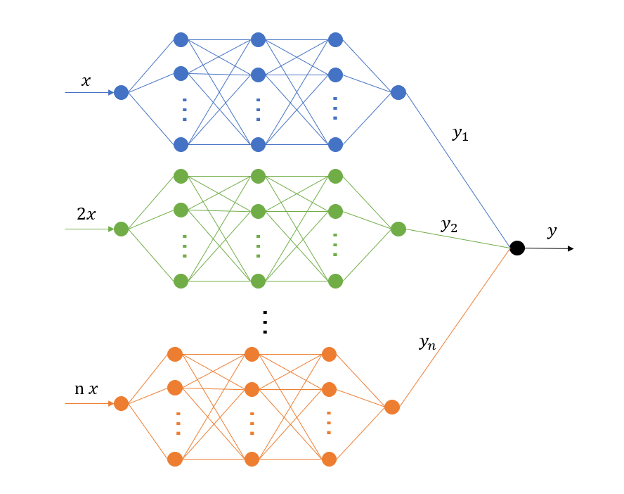
Fig. 7 shows the schematics of a MscaleDNN consisting of sub-networks. Each scaled input passing through a fully-connected sub-network, which can be expressed in the formula (22), here again we use the sine function for the activation function, i.e.,
| (45) |
Mathematically, the final output of a MscaleDNN solution is represented by the following sum of sub-networks with network parameters denoted by (i.e. weight matrices and bias)
| (46) |
where is the chosen scale vector for the -th sub-network in Fig. 7. For more details on the design of the MscaleDNN, refer to [7].
For the input scales, the general idea is to adopt various scaling factors for different components of the input, depending on the complexity of the PDE to be solved.
The MscaleDNN is tested with the following model problem, modified from the BSB equation above with an oscillatory factor to effectively increase the training difficulty:
| (47) | ||||
where the dimension , , and are unchanged parameters compared to (37),
| (48) |
| (49) |
| (50) |
where each , and , and are parameters to be tuned. The modified PDE (47) has a solution
| (51) |
and corresponds to the FBSDEs
| (52) | ||||
We apply , and to the above equation. During the training process, we use the same settings for the fully-connected DNN as in previous tests. For the MscaleDNN, the network is divided into 4 sub-networks, each having 5 hidden layers with 64 neurons per layer, so that sizes of the networks in the comparison are matching. The scaled inputs for the sub-networks are given by
| (53) |
so that a wider range of frequency of can be captured with the MscaleDNN. When applying Scheme 2 and , the MscaleDNN halves the overall error compared to the fully-connected network.
One can also predict sample paths with better accuracy using the MscaleDNN, too, see Fig. 9.
5 Conclusion
In this paper, we have proposed two FBSDE based DNN algorithms for high dimensional quasilinear parabolic equations. The key component of the proposed algorithms is the loss function used, consisting of, in addition to the terminal condition of the PDE, the pathwise difference of two convergent stochastic processes from either the discretized SDEs or the PDEs DNN solution. As the two stochastic processes converge to the same stochastic process in the Pardoux–Peng theory, the new algorithms are able to demonstrate nearly the half-order strong convergence of the underlying Euler–Maruyama scheme for the SDEs. As a result, the Richardson extrapolation method can be used, which confirms the convergence order of the DNN solutions and further enhances the resulting accuracy of the DNN solution of the PDE. For PDEs with time oscillatory solutions, the MscaleDNN is shown to provide an enhancement of the resulting accuracy as well.
Future research will be done to improve the convergence of the networks and the overall schemes, including MscaleDNN for PDEs with spatially oscillatory solutions.
References
- [1] Doob JL. Classical potential theory and its probabilistic counterpart: Advanced problems. Springer Science & Business Media; 2012 Dec 6.
- [2] Han J, Jentzen A, Weinan E. Solving high-dimensional partial differential equations using deep learning. Proceedings of the National Academy of Sciences. 2018 Aug 21;115(34):8505-10.
- [3] Han J, Long J. Convergence of the deep BSDE method for coupled FBSDEs. Probability, Uncertainty and Quantitative Risk. 2020 Dec;5(1):1-33.
- [4] El Karoui N, Peng S, Quenez MC. Backward stochastic differential equations in finance. Mathematical finance. 1997 Jan;7(1):1-71.
- [5] Karatzas I, Shreve SE. Brownian Motion and Stochastic Calculus 1998 (pp. 47-127). Springer, New York, NY.
- [6] Kloeden PE, Platen E. Numerical solution of stochastic differential equations. Springer Science & Business Media; 2013 Apr 17.
- [7] Liu, Z.Q., Wei Cai & Zhi-Qin John Xu, Multi-Scale Deep Neural Network (MscaleDNN) for Solving Poisson-Boltzmann Equation in Complex Domains. Communications in Computational Physics. 28(5), 1970-2001, 2020.
- [8] Oksendal B. Stochastic differential equations. InStochastic differential equations 2003 (pp. 65-84). Springer, Berlin, Heidelberg.
- [9] Pardoux E, Peng S. Backward stochastic differential equations and quasilinear parabolic partial differential equations. In Stochastic partial differential equations and their applications 1992 (pp. 200-217). Springer, Berlin, Heidelberg.
- [10] Pavliotis G. Stochastic Processes and Applications, 2014, Springer.
- [11] Raissi M. Forward-backward stochastic neural networks: Deep learning of high-dimensional partial differential equations. arXiv preprint arXiv:1804.07010. 2018 Apr 19.